Last observation: Q3 2012 (N = 8)
First observation: Q1 1983 (N = 4)
Last data update: 09 oct. 2026, 22:56
Last compile: 10 oct. 2026, 01:27
SERIES_LOYERS |>
  group_by(IDBANK, TITLE_FR) |>
  summarise(Nobs = n()) |>
  arrange(-Nobs) |>
print_table_conditional()| IDBANK | TITLE_FR | Nobs |
|---|---|---|
| 010600343 | Variation trimestrielle des loyers – Tous secteurs – France métropolitaine – Série arrêtée | 119 |
| 010600344 | Variation trimestrielle des loyers – Loi 1948 – France métropolitaine – Série arrêtée | 119 |
| 010600345 | Variation trimestrielle des loyers – Secteur libre – France métropolitaine – Série arrêtée | 119 |
| 010600346 | Variation trimestrielle des loyers – Secteur social – France métropolitaine – Série arrêtée | 119 |
| 010600347 | Variation annuelle des loyers – Tous secteurs – France métropolitaine – Série arrêtée | 116 |
| 010600348 | Variation annuelle des loyers – Loi 1948 – France métropolitaine – Série arrêtée | 116 |
| 010600349 | Variation annuelle des loyers – Secteur libre – France métropolitaine – Série arrêtée | 116 |
| 010600350 | Variation annuelle des loyers – Secteur social – France métropolitaine – Série arrêtée | 116 |
SERIES_LOYERS |>
  filter(SECTEURS_LOYERS == "TOUS_SECTEURS") |>
  quarter_to_date() |>
  ggplot() + ylab("Inflation des Loyers") + xlab("") + theme_minimal() +
  geom_line(aes(x = date, y = OBS_VALUE/100, color = Nature)) +
  scale_x_date(breaks = seq(1920, 2100, 2) |> paste0("-01-01") |> as.Date(),
               labels = date_format("%Y")) +
  theme(legend.position = c(0.8, 0.9),
        legend.title = element_blank()) +
  scale_y_continuous(breaks = 0.01*seq(0, 200, 1),
                     labels = percent_format(accuracy = 1))
SERIES_LOYERS |>
  filter(NATURE == "GLISSEMENT_ANNUEL") |>
  quarter_to_date() |>
  ggplot() + ylab("Inflation des Loyers") + xlab("") + theme_minimal() +
  geom_line(aes(x = date, y = OBS_VALUE/100, color = Secteurs_loyers)) +
  scale_x_date(breaks = seq(1920, 2100, 2) |> paste0("-01-01") |> as.Date(),
               labels = date_format("%Y")) +
  theme(legend.position = c(0.8, 0.85),
        legend.title = element_blank()) +
  scale_y_continuous(breaks = 0.01*seq(0, 200, 1),
                     labels = percent_format(accuracy = 1))
Les indices ci-dessous sont reconstruits en cumulant les évolutions, faute de niveau d’indice disponible dans cette table (voir INDICES_LOYERS.qmd pour les niveaux). Le GLISSEMENT_TRIMESTRIEL est chaîné directement d’un trimestre sur l’autre (méthode de l’Insee). Le GLISSEMENT_ANNUEL est disponible à fréquence trimestrielle mais mesure une évolution sur 4 trimestres : on ne garde donc qu’une observation sur 4 (un trimestre par an), ce qui donne des évolutions consécutives non chevauchantes que l’on peut chaîner directement.
bind_rows(
  SERIES_LOYERS |>
    filter(SECTEURS_LOYERS == "TOUS_SECTEURS", NATURE == "GLISSEMENT_TRIMESTRIEL") |>
    quarter_to_date() |>
    arrange(date) |>
    mutate(OBS_VALUE = 100*cumprod(1 + OBS_VALUE/100) / (1 + OBS_VALUE[1]/100)),
  SERIES_LOYERS |>
    filter(SECTEURS_LOYERS == "TOUS_SECTEURS", NATURE == "GLISSEMENT_ANNUEL") |>
    quarter_to_date() |>
    arrange(date) |>
    slice(seq(1, n(), by = 4)) |>
    mutate(OBS_VALUE = 100*cumprod(1 + OBS_VALUE/100) / (1 + OBS_VALUE[1]/100))
) |>
  ggplot() + ylab("Loyers - Tous secteurs (base 100 au 1er trimestre 1983)") + xlab("") + theme_minimal() +
  geom_line(aes(x = date, y = OBS_VALUE, color = Nature)) +
  scale_x_date(breaks = seq(1920, 2100, 2) |> paste0("-01-01") |> as.Date(),
               labels = date_format("%Y")) +
  theme(legend.position = c(0.25, 0.85),
        legend.title = element_blank()) +
  scale_y_log10(breaks = seq(0, 300, 20))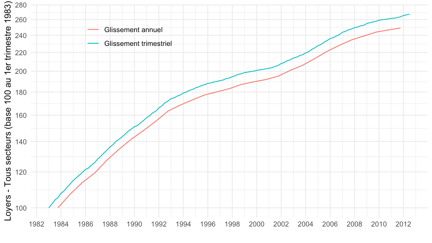
bind_rows(
  SERIES_LOYERS |>
    filter(SECTEURS_LOYERS == "TOUS_SECTEURS", NATURE == "GLISSEMENT_TRIMESTRIEL") |>
    quarter_to_date() |>
    arrange(date) |>
    mutate(OBS_VALUE = 100*cumprod(1 + OBS_VALUE/100) / (1 + OBS_VALUE[1]/100)),
  SERIES_LOYERS |>
    filter(SECTEURS_LOYERS == "TOUS_SECTEURS", NATURE == "GLISSEMENT_ANNUEL") |>
    quarter_to_date() |>
    arrange(date) |>
    slice(seq(1, n(), by = 4)) |>
    mutate(OBS_VALUE = 100*cumprod(1 + OBS_VALUE/100) / (1 + OBS_VALUE[1]/100))
) |>
  ggplot() + ylab("Loyers - Tous secteurs (100 = 1983T1)") + xlab("") + theme_minimal() +
  geom_line(aes(x = date, y = OBS_VALUE, color = Nature)) +
  scale_x_date(breaks = seq(1920, 2100, 2) |> paste0("-01-01") |> as.Date(),
               labels = date_format("%Y")) +
  theme(legend.position = c(0.25, 0.85),
        legend.title = element_blank()) +
  scale_y_log10(breaks = seq(0, 300, 20))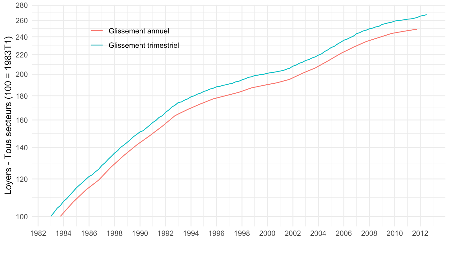
bind_rows(
  SERIES_LOYERS |>
    filter(SECTEURS_LOYERS == "TOUS_SECTEURS", NATURE == "GLISSEMENT_TRIMESTRIEL") |>
    quarter_to_date() |>
    filter(date >= as.Date("1990-01-01")) |>
    arrange(date) |>
    mutate(OBS_VALUE = 100*cumprod(1 + OBS_VALUE/100) / (1 + OBS_VALUE[1]/100)),
  SERIES_LOYERS |>
    filter(SECTEURS_LOYERS == "TOUS_SECTEURS", NATURE == "GLISSEMENT_ANNUEL") |>
    quarter_to_date() |>
    filter(date >= as.Date("1990-01-01")) |>
    arrange(date) |>
    slice(seq(1, n(), by = 4)) |>
    mutate(OBS_VALUE = 100*cumprod(1 + OBS_VALUE/100) / (1 + OBS_VALUE[1]/100))
) |>
  ggplot() + ylab("Loyers - Tous secteurs (100 = 1990T1)") + xlab("") + theme_minimal() +
  geom_line(aes(x = date, y = OBS_VALUE, color = Nature)) +
  scale_x_date(breaks = seq(1920, 2100, 2) |> paste0("-01-01") |> as.Date(),
               labels = date_format("%Y")) +
  theme(legend.position = c(0.25, 0.85),
        legend.title = element_blank()) +
  scale_y_log10(breaks = seq(0, 300, 10))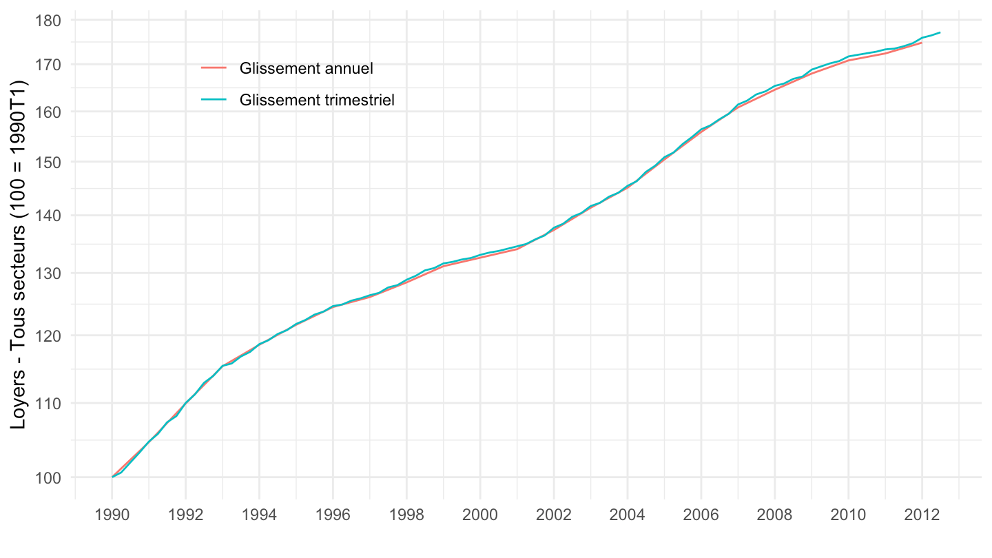
SERIES_LOYERS |>
  filter(NATURE == "GLISSEMENT_TRIMESTRIEL") |>
  quarter_to_date() |>
  arrange(date) |>
  group_by(Secteurs_loyers) |>
  mutate(OBS_VALUE = 100*cumprod(1 + OBS_VALUE/100) / (1 + OBS_VALUE[1]/100)) |>
  ungroup() |>
  ggplot() + ylab("Loyers - Glissement trimestriel (100 = 1983T1)") + xlab("") + theme_minimal() +
  geom_line(aes(x = date, y = OBS_VALUE, color = Secteurs_loyers)) +
  scale_x_date(breaks = seq(1920, 2100, 2) |> paste0("-01-01") |> as.Date(),
               labels = date_format("%Y")) +
  theme(legend.position = c(0.25, 0.85),
        legend.title = element_blank()) +
  scale_y_log10(breaks = seq(0, 300, 20))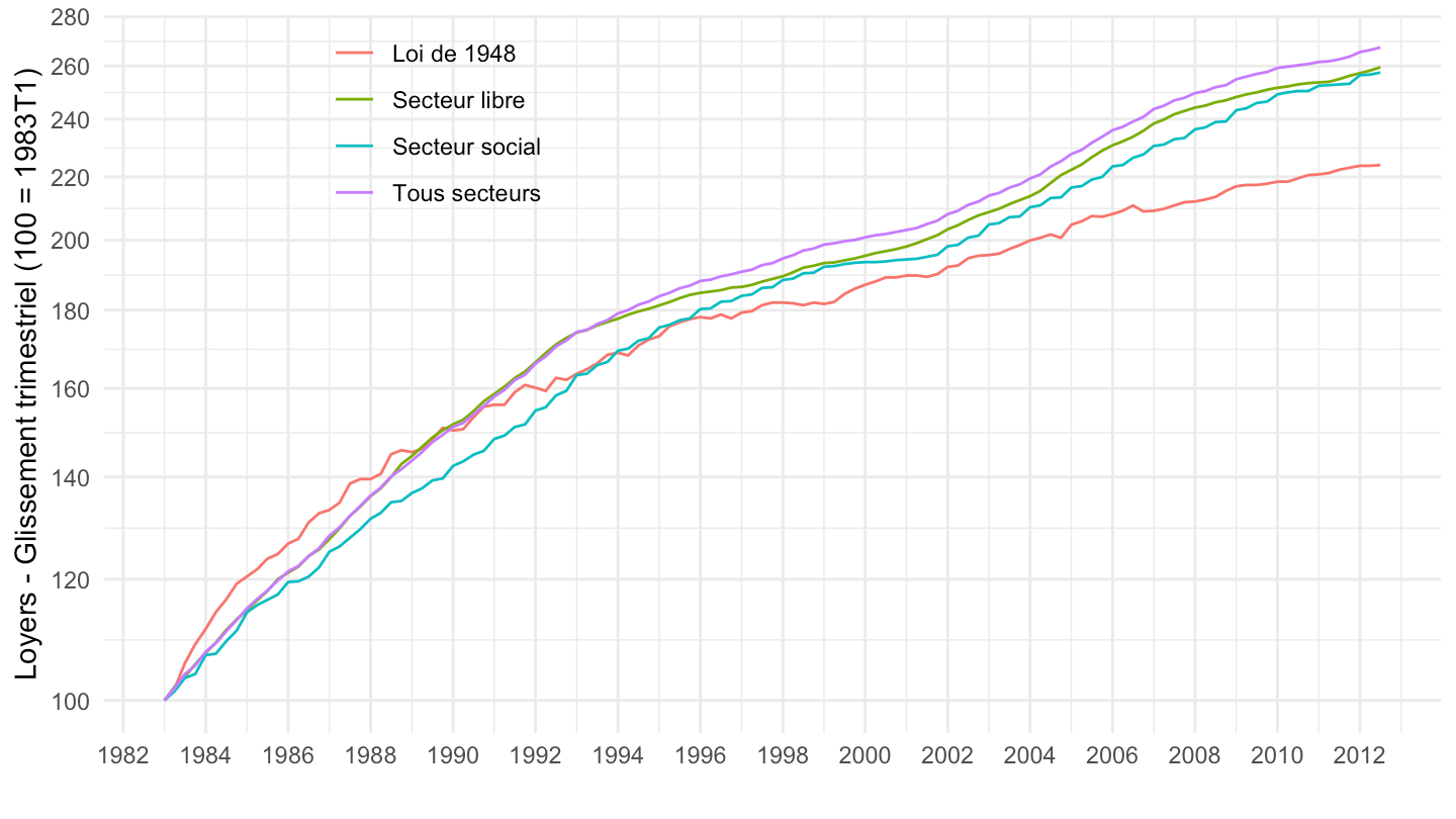
SERIES_LOYERS |>
  filter(NATURE == "GLISSEMENT_TRIMESTRIEL") |>
  quarter_to_date() |>
  filter(date >= as.Date("1990-01-01")) |>
  arrange(date) |>
  group_by(Secteurs_loyers) |>
  mutate(OBS_VALUE = 100*cumprod(1 + OBS_VALUE/100) / (1 + OBS_VALUE[1]/100)) |>
  ungroup() |>
  ggplot() + ylab("Loyers - Glissement trimestriel (100 = 1990T1)") + xlab("") + theme_minimal() +
  geom_line(aes(x = date, y = OBS_VALUE, color = Secteurs_loyers)) +
  scale_x_date(breaks = seq(1920, 2100, 2) |> paste0("-01-01") |> as.Date(),
               labels = date_format("%Y")) +
  theme(legend.position = c(0.25, 0.85),
        legend.title = element_blank()) +
  scale_y_log10(breaks = seq(0, 300, 10))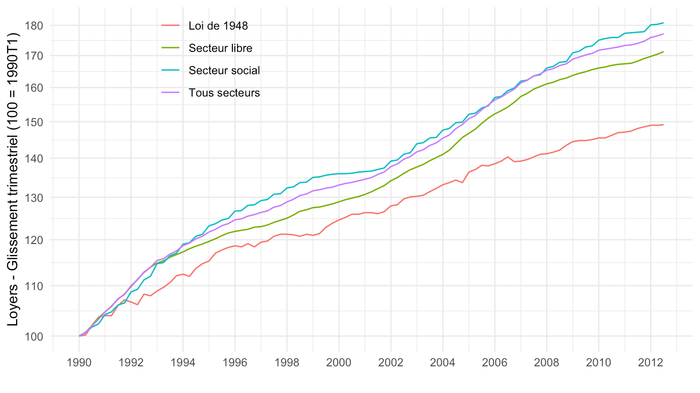
SERIES_LOYERS |>
  filter(NATURE == "GLISSEMENT_ANNUEL") |>
  quarter_to_date() |>
  arrange(date) |>
  group_by(Secteurs_loyers) |>
  slice(seq(1, n(), by = 4)) |>
  mutate(OBS_VALUE = 100*cumprod(1 + OBS_VALUE/100) / (1 + OBS_VALUE[1]/100)) |>
  ungroup() |>
  ggplot() + ylab("Loyers - Glissement annuel (100 = 1983T1)") + xlab("") + theme_minimal() +
  geom_line(aes(x = date, y = OBS_VALUE, color = Secteurs_loyers)) +
  scale_x_date(breaks = seq(1920, 2100, 2) |> paste0("-01-01") |> as.Date(),
               labels = date_format("%Y")) +
  theme(legend.position = c(0.25, 0.85),
        legend.title = element_blank()) +
  scale_y_log10(breaks = seq(0, 300, 20))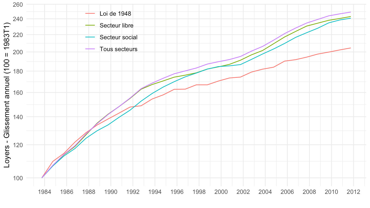
SERIES_LOYERS |>
  filter(NATURE == "GLISSEMENT_ANNUEL") |>
  quarter_to_date() |>
  filter(date >= as.Date("1990-01-01")) |>
  arrange(date) |>
  group_by(Secteurs_loyers) |>
  slice(seq(1, n(), by = 4)) |>
  mutate(OBS_VALUE = 100*cumprod(1 + OBS_VALUE/100) / (1 + OBS_VALUE[1]/100)) |>
  ungroup() |>
  ggplot() + ylab("Loyers - Glissement annuel (100 = 1990T1)") + xlab("") + theme_minimal() +
  geom_line(aes(x = date, y = OBS_VALUE, color = Secteurs_loyers)) +
  scale_x_date(breaks = seq(1920, 2100, 2) |> paste0("-01-01") |> as.Date(),
               labels = date_format("%Y")) +
  theme(legend.position = c(0.25, 0.85),
        legend.title = element_blank()) +
  scale_y_log10(breaks = seq(0, 300, 10))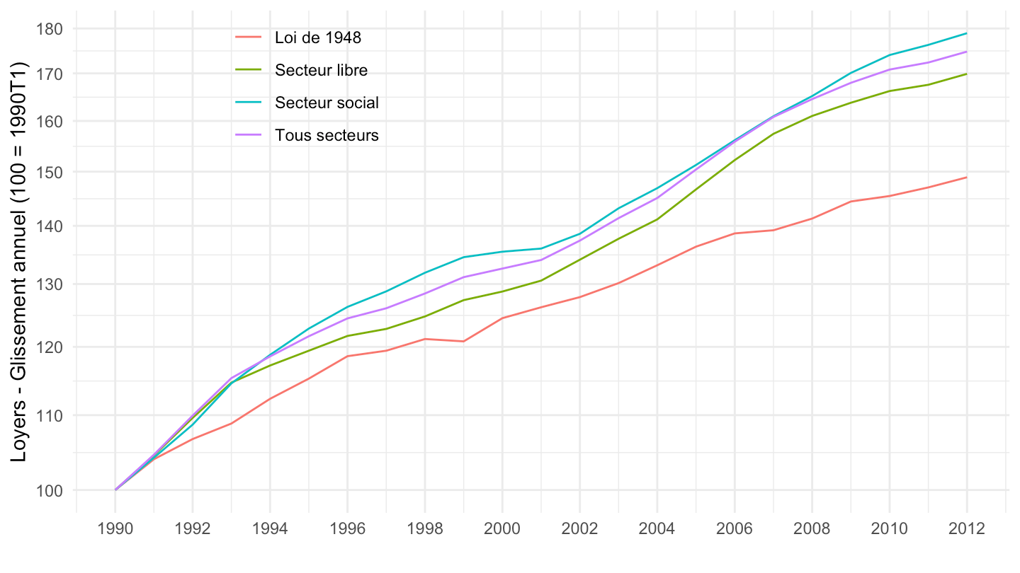
| source | dataset | Title | Updated |
|---|---|---|---|