[1] "fr_CA.UTF-8"Indice des prix à la consommation - Base 2015
Données - INSEE
Info
Last observation: 2025-12
First observation: 1990
Number of observations: 570 710
Last data update: 24 juil. 2026, 04:18. Last compile: 24 juil. 2026, 06:02
Structure
Données sur l’inflation en France
| Title | source | dataset | .html | .RData |
|---|---|---|---|---|
| Budget de famille 2017 | insee | bdf2017 | 2026-07-24 | 2023-11-21 |
| Échantillon d’agglomérations enquêtées de l’IPC en 2024 | insee | echantillon-agglomerations-IPC-2024 | 2026-07-24 | 2026-01-27 |
| Échantillon d’agglomérations enquêtées de l’IPC en 2025 | insee | echantillon-agglomerations-IPC-2025 | 2026-07-24 | 2026-01-27 |
| Indices pour la révision d’un bail commercial ou professionnel | insee | ILC-ILAT-ICC | 2026-07-24 | NA |
| Indices des loyers d'habitation (ILH) | insee | INDICES_LOYERS | 2026-07-24 | 2026-07-24 |
| Indice des prix à la consommation - Base 1970, 1980 | insee | IPC-1970-1980 | 2026-07-24 | NA |
| Indices des prix à la consommation - Base 1990 | insee | IPC-1990 | 2026-07-24 | NA |
| Indice des prix à la consommation - Base 2015 | insee | IPC-2015 | 2026-07-24 | 2026-07-23 |
| Prix moyens de vente de détail | insee | IPC-PM-2015 | 2026-07-24 | NA |
| Indices des prix à la consommation harmonisés | insee | IPCH-2015 | 2026-07-24 | 2026-07-24 |
| Indices des prix à la consommation harmonisés | insee | IPCH-IPC-2015-ensemble | 2026-07-23 | 2026-07-24 |
| Indice des prix dans la grande distribution | insee | IPGD-2015 | 2026-07-24 | NA |
| Indices des prix des logements neufs et Indices Notaires-Insee des prix des logements anciens | insee | IPLA-IPLNA-2015 | 2026-07-24 | NA |
| Indices de prix de production et d'importation dans l'industrie | insee | IPPI-2015 | 2026-07-24 | NA |
| Indice pour la révision d’un loyer d’habitation | insee | IRL | 2026-07-24 | 2026-07-23 |
| Liste des variétés pour la mesure de l'IPC en 2024 | insee | liste-varietes-IPC-2024 | 2026-07-23 | 2025-04-02 |
| Liste des variétés pour la mesure de l'IPC en 2025 | insee | liste-varietes-IPC-2025 | 2026-07-23 | 2026-01-27 |
| Pondérations élémentaires 2024 intervenant dans le calcul de l’IPC | insee | ponderations-elementaires-IPC-2024 | 2026-07-23 | 2025-04-02 |
| Pondérations élémentaires 2025 intervenant dans le calcul de l’IPC | insee | ponderations-elementaires-IPC-2025 | 2026-07-23 | 2026-01-27 |
| Variation des loyers | insee | SERIES_LOYERS | 2026-07-23 | 2026-07-23 |
| Consommation effective des ménages par fonction | insee | T_CONSO_EFF_FONCTION | 2026-07-23 | 2025-12-22 |
| Montants de consommation selon différentes catégories de ménages | insee | table_conso_moyenne_par_categorie_menages | 2026-07-23 | 2026-01-27 |
| Ventilation de chaque sous-classe (niveau 4 de la COICOP v2) en postes et leurs pondérations | insee | table_poste_au_sein_sous_classe_ecoicopv2_france_entiere_ | 2026-07-23 | 2026-01-27 |
| Poids de chaque tranche d’unités urbaines dans la consommation | insee | tranches_unitesurbaines | 2026-07-23 | 2026-01-27 |
LAST_COMPILE
| LAST_COMPILE |
|---|
| 2026-07-24 |
Definitions
Moyenne annuelle: l’évolution en moyenne annuelle compare les prix d’une année donnée à ceux de l’année précédente.
Glissement annuel: l’évolution en glissement annuel compare les prix d’un seul mois d’une année donnée à ceux du même mois de l’année précédente.
Méthodo
- Indice des prix à la consommation (base 100=1998) (pdf, fr, 44 Ko, 01/02/2013)
- Indice des prix à la consommation des ménages du premier quintile de la distribution des niveaux de vie (pdf, fr, 119 Ko, 18/02/2013)
- Indice des prix à la consommation (base 100=2015) (pdf, fr, 145 Ko, 29/01/2016)
- Indice des prix à la consommation des ménages - base 100 en 2015 (pdf, fr, 955 Ko, 29/01/2016)
- Pour comprendre l’indice des prix - Édition 1998 (pdf, fr, 1 Mo, 01/01/1999)
- Indice des prix à la consommation des ménages - base 100 en 1998 (pdf, fr, 50 Ko, 01/01/1999)
- Dossier d’information méthodologique. Indice des prix, pouvoir d’achat (pdf, fr, 229 Ko, 01/02/2004)
Documents de travail
- L’IPC, miroir de l’évolution du coût de la vie en France ? - Ce qu’apporte l’analyse des courbes d’Engel. (pdf, fr, 615 Ko, 02/04/2010)
- Calcul d’un indice des prix des produits de grande consommation dans la grande distribution (pdf, fr, 204 Ko, 01/01/2014)
- Ce qui change pour l’IPC à partir du 29 janvier 2016 (pdf, fr, 129 Ko, 29/01/2016)
- L’expérience française des indices de prix a la consommation (pdf, fr, 107 Ko, 01/01/1996) Indice des prix à la consommation CVS et indice hors tarifs publics et produits à prix volatils corrigé des mesures fiscales, CVS (pdf, fr, 71 Ko, 27/03/1996)
- Indices mensuels des prix dans la grande distribution (pdf, fr, 126 Ko, 18/02/2016)
- Contenu des groupes avec les fonctions, les regroupements et les groupes publiés dans la nouvelle base 1998 (pdf, fr, 42 Ko, 01/01/1999)
- Comparaisons spatiales de prix au sein du territoire français (pdf, fr, 91 Ko, 01/12/2000)
- Les indices à utilité constante : une référence pour mesurer l’évolution des prix (pdf, fr, 219 Ko, 01/12/2000)
- La mesure des prix dans les domaines de la santé et de l’action sociale : quelques problèmes méthodologiques (pdf, fr, 212 Ko, 01/06/2003)
- Indice des prix à la consommation en base 100 en 1998 - Séries longues rétropolées, de 1990 à 2002 (pdf, fr, 201 Ko, 01/09/2003)
- Impact des ajustements de qualité dans le calcul de l’indice des prix à la consommation (pdf, fr, 53 Ko, 01/05/2004)
- Introduction à la pratique des indices statistiques (pdf, fr, 426 Ko, 01/11/2005)
- Note additionnelle sur les changements de l’année 2017 (pdf, fr, 228 Ko, 23/02/2017)
TEF 2020
Code
ig_b("insee", "TEF2020", "114-IPC-poids")
Depuis 2017
2-digit
Code
`IPC-2015` %>%
  filter(nchar(COICOP2016) == 2) %>%

  group_by(COICOP2016, Coicop2016) %>%
  filter(FREQ == "M",
         TIME_PERIOD %in% c("2017-01", "2025-12"),
         COICOP2016 != "SO",
         MENAGES_IPC == "ENSEMBLE",
         NATURE == "INDICE",
         REF_AREA == "FE",
         PRIX_CONSO == "SO") %>%
  arrange(COICOP2016, Coicop2016) %>%
  select(TIME_PERIOD, OBS_VALUE) %>%
  spread(TIME_PERIOD, OBS_VALUE) %>%
  mutate(`%` = round(100*((`2025-12`/`2017-01`)-1), 1)) %>%
  arrange(- `%`) %>%
print_table_conditional()| COICOP2016 | Coicop2016 | 2017-01 | 2025-12 | % |
|---|---|---|---|---|
| 02 | 02 - Boissons alcoolisées, tabac et stupéfiants | 100.59 | 154.23 | 53.3 |
| 01 | 01 - Produits alimentaires et boissons non alcoolisées | 101.23 | 135.46 | 33.8 |
| 04 | 04 - Logement, eau, gaz, électricité et autres combustibles | 101.56 | 131.30 | 29.3 |
| 07 | 07 - Transports | 101.66 | 126.64 | 24.6 |
| 11 | 11 - Restaurants et hôtels | 101.68 | 125.61 | 23.5 |
| 12 | 12 - Biens et services divers | 101.63 | 124.20 | 22.2 |
| 00 | 00 - Ensemble | 100.41 | 120.90 | 20.4 |
| 10 | 10 - Enseignement | 102.31 | 122.86 | 20.1 |
| 03 | 03 - Articles d'habillement et chaussures | 92.55 | 108.80 | 17.6 |
| 05 | 05 - Meubles, articles de ménage et entretien courant du foyer | 98.86 | 114.47 | 15.8 |
| 09 | 09 - Loisirs et culture | 100.31 | 109.83 | 9.5 |
| 06 | 06 - Santé | 98.44 | 94.12 | -4.4 |
| 08 | 08 - Communications | 97.34 | 76.24 | -21.7 |
3-digit
Code
`IPC-2015` %>%
  filter(nchar(COICOP2016) == 3) %>%

  group_by(COICOP2016, Coicop2016) %>%
  filter(FREQ == "M",
         TIME_PERIOD %in% c("2017-01", "2025-12"),
         COICOP2016 != "SO",
         MENAGES_IPC == "ENSEMBLE",
         NATURE == "INDICE",
         REF_AREA == "FE",
         PRIX_CONSO == "SO") %>%
  arrange(COICOP2016, Coicop2016) %>%
  select(TIME_PERIOD, OBS_VALUE) %>%
  spread(TIME_PERIOD, OBS_VALUE) %>%
  mutate(`%` = round(100*((`2025-12`/`2017-01`)-1), 1)) %>%
  arrange(- `%`) %>%
  print_table_conditional()
4-digit
Code
`IPC-2015` %>%
  filter(nchar(COICOP2016) == 4) %>%

  group_by(COICOP2016, Coicop2016) %>%
  filter(FREQ == "M",
         TIME_PERIOD %in% c("2017-01", "2025-12"),
         COICOP2016 != "SO",
         MENAGES_IPC == "ENSEMBLE",
         NATURE == "INDICE",
         REF_AREA == "FE",
         PRIX_CONSO == "SO") %>%
  arrange(COICOP2016, Coicop2016) %>%
  select(TIME_PERIOD, OBS_VALUE) %>%
  spread(TIME_PERIOD, OBS_VALUE) %>%
  mutate(`%` = round(100*((`2025-12`/`2017-01`)-1), 1)) %>%
  arrange(- `%`) %>%
  print_table_conditional()
5-digit
Code
`IPC-2015` %>%
  filter(nchar(COICOP2016) == 5) %>%

  group_by(COICOP2016, Coicop2016) %>%
  filter(FREQ == "M",
         TIME_PERIOD %in% c("2017-01", "2025-12"),
         COICOP2016 != "SO",
         MENAGES_IPC == "ENSEMBLE",
         NATURE == "INDICE",
         REF_AREA == "FE",
         PRIX_CONSO == "SO") %>%
  arrange(COICOP2016, Coicop2016) %>%
  select(TIME_PERIOD, OBS_VALUE) %>%
  spread(TIME_PERIOD, OBS_VALUE) %>%
  mutate(`%` = round(100*((`2025-12`/`2017-01`)-1), 1)) %>%
  arrange(- `%`) %>%
  print_table_conditional()
6-digit
Code
`IPC-2015` %>%
  filter(nchar(COICOP2016) == 6) %>%

  group_by(COICOP2016, Coicop2016) %>%
  filter(FREQ == "A",
         TIME_PERIOD %in% c("2017", "2025"),
         COICOP2016 != "SO",
         MENAGES_IPC == "ENSEMBLE",
         NATURE == "INDICE",
         REF_AREA == "FE",
         PRIX_CONSO == "SO") %>%
  arrange(COICOP2016, Coicop2016) %>%
  select(TIME_PERIOD, OBS_VALUE) %>%
  spread(TIME_PERIOD, OBS_VALUE) %>%
  mutate(`%` = round(100*((`2025`/`2017`)-1), 1)) %>%
  arrange(- `%`) %>%
  print_table_conditional()
6 -digit plus forts
Problèmes méthodologiques
Code
`IPC-2015` %>%
  filter(nchar(COICOP2016) == 6) %>%

  group_by(COICOP2016, Coicop2016) %>%
  filter(FREQ == "A",
         COICOP2016 %in% c("082021", "062312", "083021", "091122", "091311"),
         MENAGES_IPC == "ENSEMBLE",
         NATURE == "INDICE",
         REF_AREA == "FE",
         PRIX_CONSO == "SO") %>%
  year_to_date %>%
  filter(date >= as.Date("2017-01-01")) %>%
  group_by(COICOP2016) %>%
  arrange(date) %>%
  mutate(OBS_VALUE = 100*OBS_VALUE/OBS_VALUE[1]) %>%
  ggplot() + ylab("Indice des prix") + xlab("") + theme_minimal() +
  geom_line(aes(x = date, y = OBS_VALUE, color = Coicop2016)) +

  scale_x_date(breaks = seq(1920, 2100, 1) %>% paste0("-01-01") %>% as.Date,
               labels = date_format("%Y")) +
  theme(legend.position = c(0.25, 0.25),
        legend.title = element_blank()) +
  scale_y_log10(breaks = seq(0, 200, 5),
                     labels = dollar_format(accuracy = 1, prefix = ""))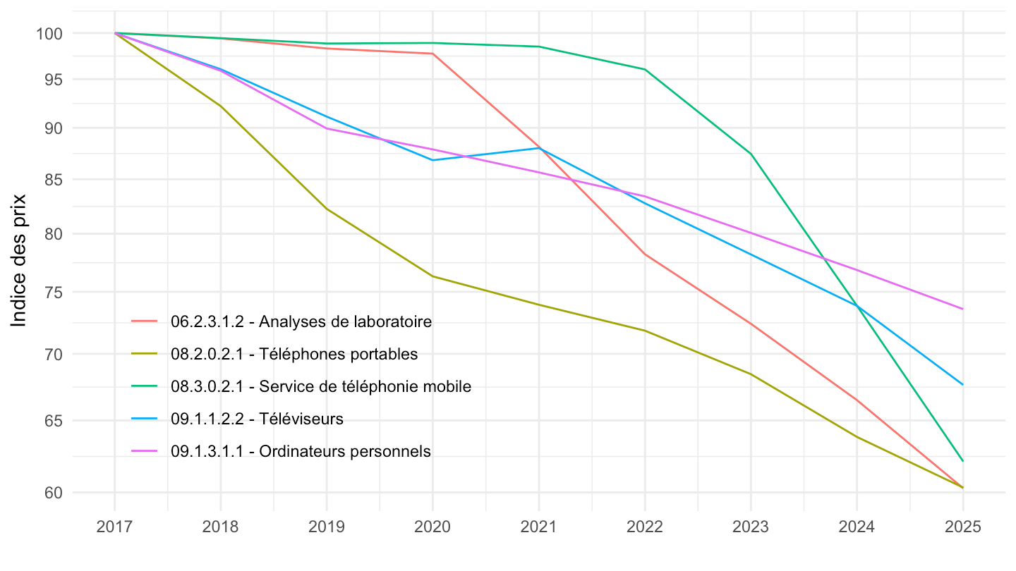
Remplacements pour l’habillement ?
Code
`IPC-2015` %>%
  filter(nchar(COICOP2016) == 6) %>%

  group_by(COICOP2016, Coicop2016) %>%
  filter(FREQ == "A",
         COICOP2016 %in% c("031236", "031234", "031238", "031233", "031237"),
         MENAGES_IPC == "ENSEMBLE",
         NATURE == "INDICE",
         REF_AREA == "FE",
         PRIX_CONSO == "SO") %>%
  year_to_date %>%
  filter(date >= as.Date("2017-01-01")) %>%
  group_by(COICOP2016) %>%
  arrange(date) %>%
  mutate(OBS_VALUE = 100*OBS_VALUE/OBS_VALUE[1]) %>%
  ggplot() + ylab("Indice des prix") + xlab("") + theme_minimal() +
  geom_line(aes(x = date, y = OBS_VALUE, color = Coicop2016)) +

  scale_x_date(breaks = seq(1920, 2100, 1) %>% paste0("-01-01") %>% as.Date,
               labels = date_format("%Y")) +
  theme(legend.position = c(0.35, 0.25),
        legend.title = element_blank()) +
  scale_y_log10(breaks = seq(0, 200, 1),
                     labels = dollar_format(accuracy = 1, prefix = ""))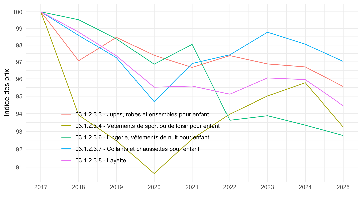
France Entiere (FE), France Métropolitaine (FM)
1990-
Code
`IPC-2015` %>%
  filter(INDICATEUR == "IPC",
         MENAGES_IPC == "ENSEMBLE",
         PRIX_CONSO %in% c("SO"),
         FREQ == "M",
         COICOP2016 %in% c("00"),
         REF_AREA %in% c("FE", "FM"),
         NATURE == "INDICE") %>%
  month_to_date %>%
  arrange(desc(date)) %>%
  group_by(REF_AREA) %>%
  arrange(date) %>%
  mutate(OBS_VALUE = 100*OBS_VALUE/OBS_VALUE[1]) %>%
  ggplot() + ylab("Indice des prix") + xlab("") + theme_minimal() +
  geom_line(aes(x = date, y = OBS_VALUE, color = REF_AREA)) +

  scale_x_date(breaks = seq(1920, 2100, 5) %>% paste0("-01-01") %>% as.Date,
               labels = date_format("%Y")) +
  theme(legend.position = c(0.75, 0.3),
        legend.title = element_blank()) +
  scale_y_log10(breaks = seq(0, 200, 10),
                     labels = dollar_format(accuracy = 1, prefix = "")) +
  geom_text_repel(data = . %>%
              filter(date == max(date)), aes(x = date, y = OBS_VALUE, label = round(OBS_VALUE, 1)), size = 3)
1996-
Code
`IPC-2015` %>%
  filter(INDICATEUR == "IPC",
         MENAGES_IPC == "ENSEMBLE",
         PRIX_CONSO %in% c("SO"),
         FREQ == "M",
         COICOP2016 %in% c("00"),
         REF_AREA %in% c("FE", "FM"),
         NATURE == "INDICE") %>%
  month_to_date %>%
  filter(date >= as.Date("1996-01-01")) %>%
  arrange(desc(date)) %>%
  group_by(REF_AREA) %>%
  arrange(date) %>%
  mutate(OBS_VALUE = 100*OBS_VALUE/OBS_VALUE[1]) %>%
  ggplot() + ylab("Indice des prix") + xlab("") + theme_minimal() +
  geom_line(aes(x = date, y = OBS_VALUE, color = REF_AREA)) +

  scale_x_date(breaks = seq(1920, 2100, 2) %>% paste0("-01-01") %>% as.Date,
               labels = date_format("%Y")) +
  theme(legend.position = c(0.75, 0.3),
        legend.title = element_blank()) +
  scale_y_log10(breaks = seq(0, 200, 10),
                     labels = dollar_format(accuracy = 1, prefix = "")) +
  geom_text_repel(data = . %>%
              filter(date == max(date)), aes(x = date, y = OBS_VALUE, label = round(OBS_VALUE, 1)), size = 3)
Alimentation, loyers, chauffage, Ensemble
2017-
Code
`IPC-2015` %>%
  filter(INDICATEUR == "IPC",
         COICOP2016 %in% c("041", "00", "01", "045"),
         FREQ == "M",
         REF_AREA == "FM",
         NATURE == "INDICE") %>%
  month_to_date %>%

  filter(date >= as.Date("2017-01-01")) %>%
  group_by(COICOP2016) %>%
  arrange(date) %>%
  mutate(OBS_VALUE = 100*OBS_VALUE/OBS_VALUE[1]) %>%
  ggplot() + ylab("Indice des prix") + xlab("") + theme_minimal() +
  geom_line(aes(x = date, y = OBS_VALUE, color = Coicop2016)) +
  theme_minimal() + xlab("") + ylab("") +
  scale_x_date(breaks = "6 months",
               labels = date_format("%b %Y")) +
  theme(legend.position = c(0.35, 0.8),
        legend.title = element_blank(),
        axis.text.x = element_text(angle = 45, vjust = 0.5, hjust=1)) +
  scale_y_log10(breaks = seq(100, 200, 5)) +
  geom_label(data = . %>%
              filter(date == max(date)), aes(x = date, y = OBS_VALUE, label = round(OBS_VALUE, 1), color = Coicop2016), size = 3)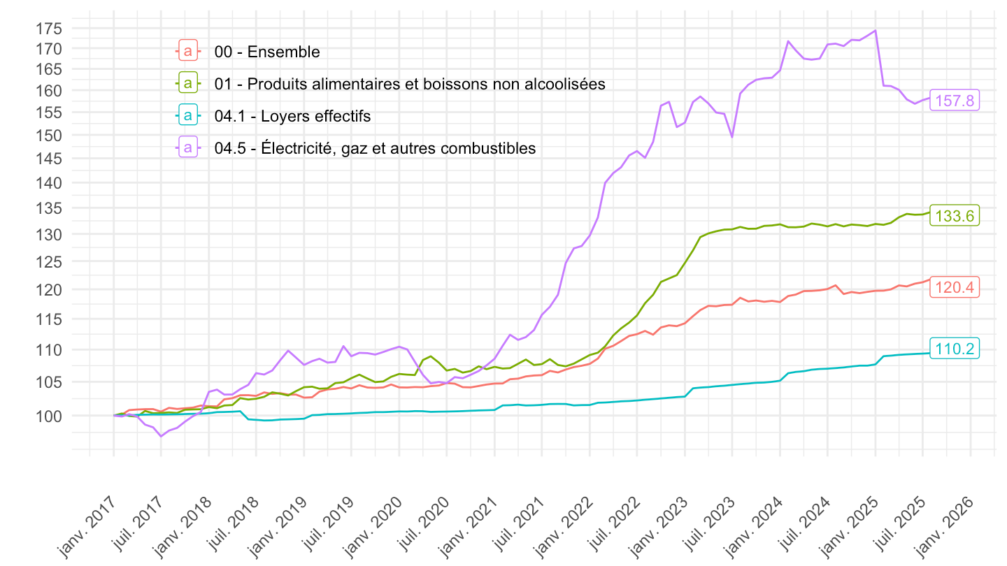
Hausse sur 2 ans
Code
`IPC-2015` %>%
  filter(INDICATEUR == "IPC",
         COICOP2016 %in% c("041", "00", "01", "045"),
         FREQ == "M",
         REF_AREA == "FM",
         NATURE == "INDICE") %>%
  month_to_date %>%

  filter(date >= max(date) - years(2)) %>%
  group_by(COICOP2016) %>%
  arrange(date) %>%
  mutate(OBS_VALUE = 100*OBS_VALUE/OBS_VALUE[1]) %>%
  ggplot() + ylab("Indice des prix") + xlab("") + theme_minimal() +
  geom_line(aes(x = date, y = OBS_VALUE, color = Coicop2016)) +
  theme_minimal() + xlab("") + ylab("") +
  scale_x_date(breaks = "1 month",
               labels = date_format("%b %Y")) +
  theme(legend.position = c(0.28, 0.87),
        legend.title = element_blank(),
        axis.text.x = element_text(angle = 45, vjust = 0.5, hjust=1)) +
  scale_y_log10(breaks = seq(100, 130, 2),
                labels = paste0(seq(0, 30, 2), "%")) +
  geom_text_repel(data = . %>%
              filter(date == max(date)), aes(x = date, y = OBS_VALUE, label = round(OBS_VALUE, 1)), size = 3)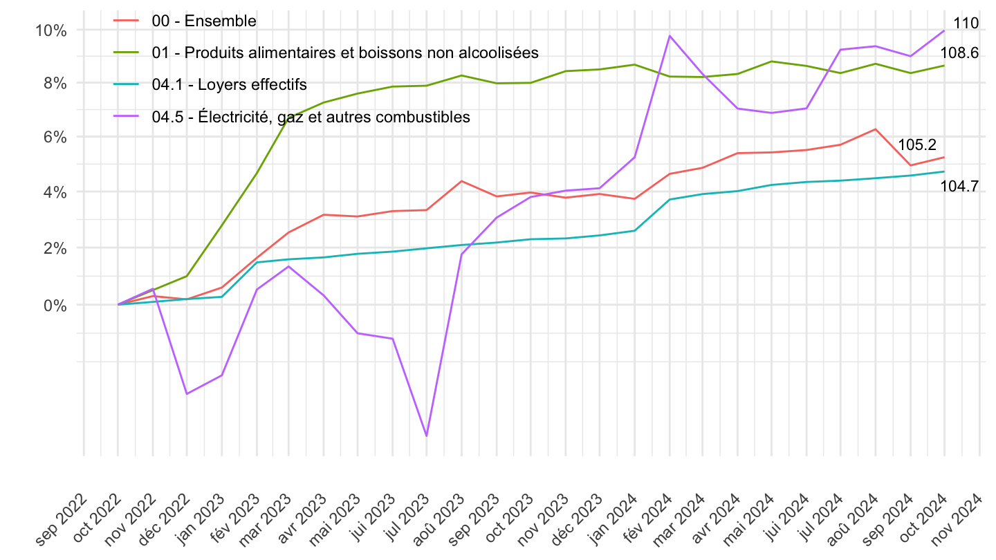
Par type de ménages
3 déciles
Code
`IPC-2015` %>%
  filter(MENAGES_IPC %in% c("D6-D7", "INF-D1", "D9-PLUS")) %>%

  year_to_date %>%
  group_by(MENAGES_IPC) %>%
  arrange(date) %>%
  mutate(OBS_VALUE = 100*OBS_VALUE/OBS_VALUE[1]) %>%
  ggplot + geom_line(aes(x = date, y = OBS_VALUE, color = Menages_ipc)) +
  theme_minimal() + xlab("") + ylab("") +
  scale_x_date(breaks = seq(1920, 2100, 2) %>% paste0("-01-01") %>% as.Date,
               labels = date_format("%Y")) +
  theme(legend.position = c(0.7, 0.2),
        legend.title = element_blank()) +
  scale_y_log10(breaks = seq(0, 200, 5),
                     labels = dollar_format(accuracy = 1, prefix = "")) +
  geom_text_repel(data = . %>%
              filter(date == max(date)), aes(x = date, y = OBS_VALUE, label = round(OBS_VALUE, 1)), size = 3)
10 dixièmes
1998-
Code
`IPC-2015` %>%
  filter(MENAGES_IPC %in% c("INF-D1", "D1-D2", "D2-D3", "D3-D4", "D4-D5",
                            "D5-D6", "D6-D7", "D7-D8", "D8-D9", "D9-PLUS")) %>%

  year_to_date %>%
  group_by(MENAGES_IPC) %>%
  mutate(MENAGES_IPC = factor(MENAGES_IPC, levels = c("INF-D1", "D1-D2", "D2-D3", "D3-D4", "D4-D5",
                            "D5-D6", "D6-D7", "D7-D8", "D8-D9", "D9-PLUS"))) %>%
  arrange(date) %>%
  mutate(OBS_VALUE = 100*OBS_VALUE/OBS_VALUE[1]) %>%
  ggplot + geom_line(aes(x = date, y = OBS_VALUE, color = MENAGES_IPC)) +
  theme_minimal() + xlab("") + ylab("") +
  scale_x_date(breaks = seq(1920, 2100, 2) %>% paste0("-01-01") %>% as.Date,
               labels = date_format("%Y")) +
  theme(legend.position = c(0.25, 0.7),
        legend.title = element_blank()) +
  guides(color = guide_legend(ncol = 3)) +
  scale_y_log10(breaks = seq(0, 200, 5),
                     labels = dollar_format(accuracy = 1, prefix = ""))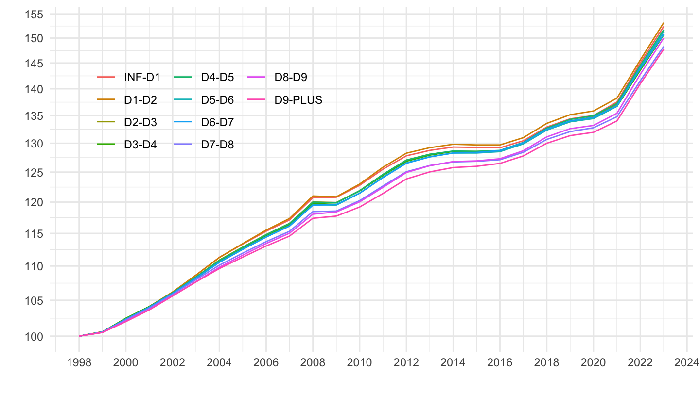
2008-
Code
`IPC-2015` %>%
  filter(MENAGES_IPC %in% c("INF-D1", "D1-D2", "D2-D3", "D3-D4", "D4-D5",
                            "D5-D6", "D6-D7", "D7-D8", "D8-D9", "D9-PLUS")) %>%

  year_to_date %>%
  group_by(MENAGES_IPC) %>%
  mutate(MENAGES_IPC = factor(MENAGES_IPC,
                              levels = c("INF-D1", "D1-D2", "D2-D3", "D3-D4", "D4-D5",
                                         "D5-D6", "D6-D7", "D7-D8", "D8-D9", "D9-PLUS"))) %>%
  arrange(date) %>%
  filter(date >= as.Date("2008-01-01")) %>%
  mutate(OBS_VALUE = 100*OBS_VALUE/OBS_VALUE[1]) %>%
  ggplot + geom_line(aes(x = date, y = OBS_VALUE, color = MENAGES_IPC)) +
  theme_minimal() + xlab("") + ylab("") +
  scale_x_date(breaks = seq(1920, 2100, 2) %>% paste0("-01-01") %>% as.Date,
               labels = date_format("%Y")) +
  theme(legend.position = c(0.25, 0.7),
        legend.title = element_blank()) +
  guides(color = guide_legend(ncol = 3)) +
  scale_y_log10(breaks = seq(0, 200, 2),
                     labels = dollar_format(accuracy = 1, prefix = ""))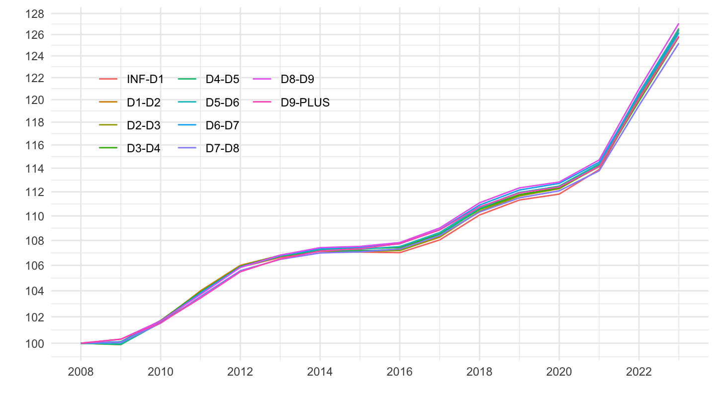
1er quintile, Tous
All
Code
`IPC-2015` %>%
  filter(MENAGES_IPC %in% c("PREMIERQUINTILE", "ENSEMBLE"),
         FREQ == "M",
         PRIX_CONSO == "4018",
         REF_AREA == "FE",
         COICOP2016 == "SO",
         NATURE == "INDICE") %>%

  month_to_date %>%
  ggplot + geom_line(aes(x = date, y = OBS_VALUE, color = Menages_ipc)) +
  theme_minimal() + xlab("") + ylab("") +
  scale_x_date(breaks = seq(1920, 2100, 2) %>% paste0("-01-01") %>% as.Date,
               labels = date_format("%Y")) +
  theme(legend.position = c(0.7, 0.2),
        legend.title = element_blank()) +
  scale_y_log10(breaks = seq(0, 200, 5),
                     labels = dollar_format(accuracy = 1, prefix = ""))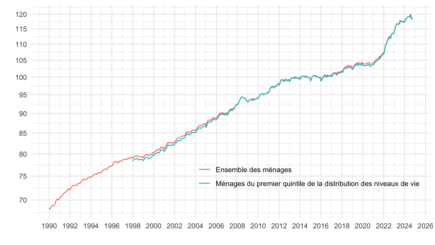
1998-
Code
`IPC-2015` %>%
  filter(MENAGES_IPC %in% c("PREMIERQUINTILE", "ENSEMBLE"),
         FREQ == "M",
         PRIX_CONSO == "4018",
         REF_AREA == "FE",
         COICOP2016 == "SO",
         NATURE == "INDICE") %>%

  month_to_date %>%
  filter(date >= as.Date("1998-01-01")) %>%
  group_by(MENAGES_IPC) %>%
  arrange(date) %>%
  mutate(OBS_VALUE = 100*OBS_VALUE/OBS_VALUE[1]) %>%
  ggplot + geom_line(aes(x = date, y = OBS_VALUE, color = Menages_ipc)) +
  theme_minimal() + xlab("") + ylab("") +
  scale_x_date(breaks = seq(1920, 2100, 2) %>% paste0("-01-01") %>% as.Date,
               labels = date_format("%Y")) +
  theme(legend.position = c(0.6, 0.2),
        legend.title = element_blank()) +
  scale_y_log10(breaks = seq(0, 200, 5),
                     labels = dollar_format(accuracy = 1, prefix = ""))
2012-
Code
`IPC-2015` %>%
  filter(MENAGES_IPC %in% c("PREMIERQUINTILE", "ENSEMBLE"),
         FREQ == "M",
         PRIX_CONSO == "4018",
         REF_AREA == "FE",
         COICOP2016 == "SO",
         NATURE == "INDICE") %>%

  month_to_date %>%
  filter(date >= as.Date("2012-01-01")) %>%
  group_by(MENAGES_IPC) %>%
  arrange(date) %>%
  mutate(OBS_VALUE = 100*OBS_VALUE/OBS_VALUE[1]) %>%
  ggplot + geom_line(aes(x = date, y = OBS_VALUE, color = Menages_ipc)) +
  theme_minimal() + xlab("") + ylab("") +
  scale_x_date(breaks = seq(1920, 2100, 2) %>% paste0("-01-01") %>% as.Date,
               labels = date_format("%Y")) +
  theme(legend.position = c(0.4, 0.9),
        legend.title = element_blank()) +
  scale_y_log10(breaks = seq(0, 200, 2),
                     labels = dollar_format(accuracy = 1, prefix = "")) +
  geom_text_repel(data = . %>%
              filter(date == max(date)), aes(x = date, y = OBS_VALUE, label = round(OBS_VALUE, 1)), size = 3)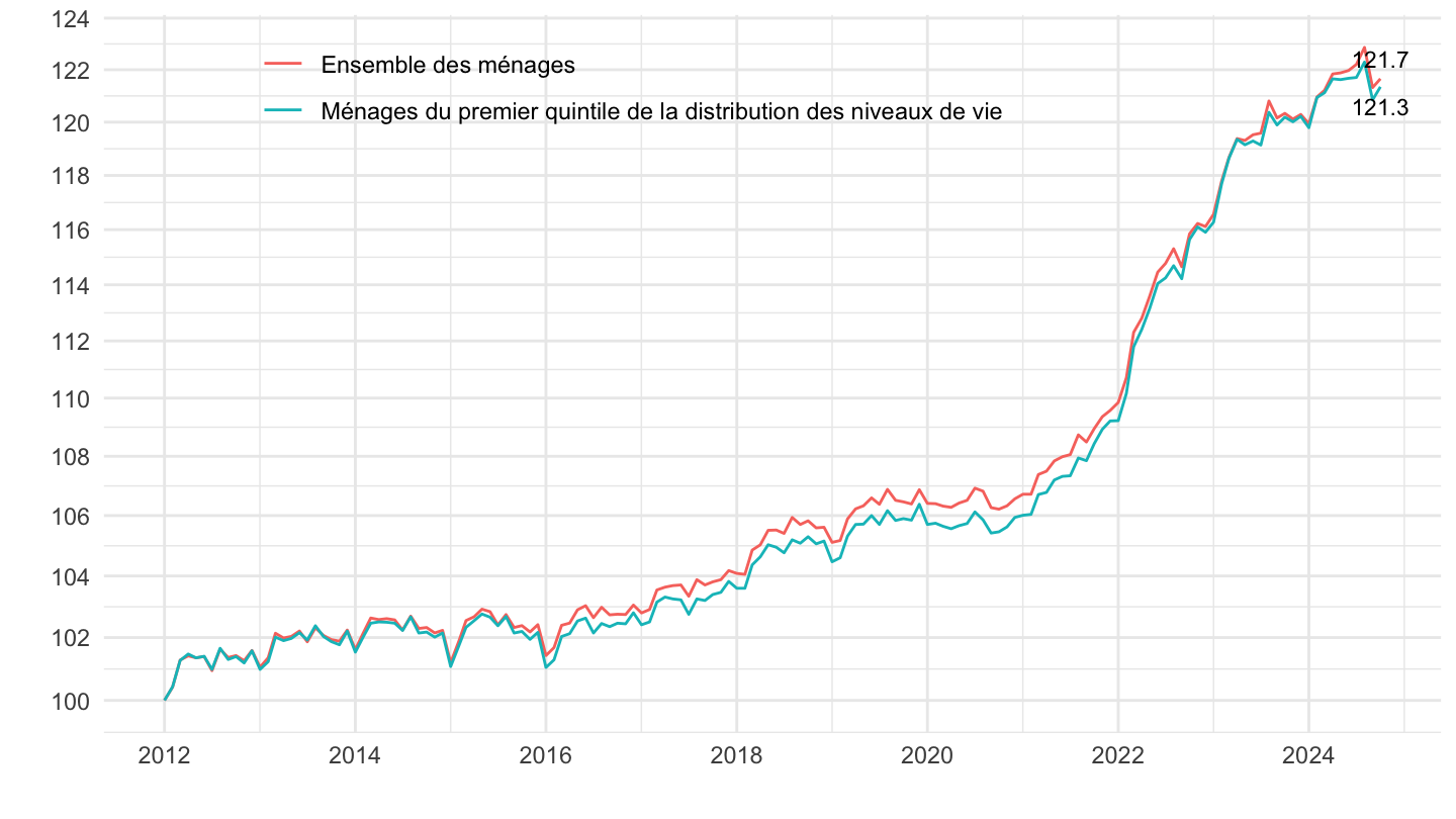
Glissement sur 2 ans
Code
`IPC-2015` %>%
  filter(MENAGES_IPC %in% c("PREMIERQUINTILE", "ENSEMBLE"),
         FREQ == "M",
         PRIX_CONSO == "4018",
         REF_AREA == "FE",
         COICOP2016 == "SO",
         NATURE == "INDICE") %>%

  month_to_date %>%
  filter(date >= as.Date("2021-09-01")) %>%
  group_by(MENAGES_IPC) %>%
  arrange(date) %>%
  mutate(OBS_VALUE = 100*OBS_VALUE/OBS_VALUE[1]) %>%
  ggplot + geom_line(aes(x = date, y = OBS_VALUE, color = Menages_ipc)) +
  theme_minimal() + xlab("") + ylab("") +
  scale_x_date(breaks = "1 month",
               labels = date_format("%b %Y")) +
  theme(legend.position = c(0.65, 0.2),
        legend.title = element_blank(),
        axis.text.x = element_text(angle = 45, vjust = 0.5, hjust=1)) +
  scale_y_log10(breaks = seq(0, 200, 1),
                     labels = dollar_format(accuracy = 1, prefix = "")) +
  geom_text_repel(aes(x = date, y = OBS_VALUE, label = round(OBS_VALUE, 1)),
                  fontface ="plain", color = "black", size = 3)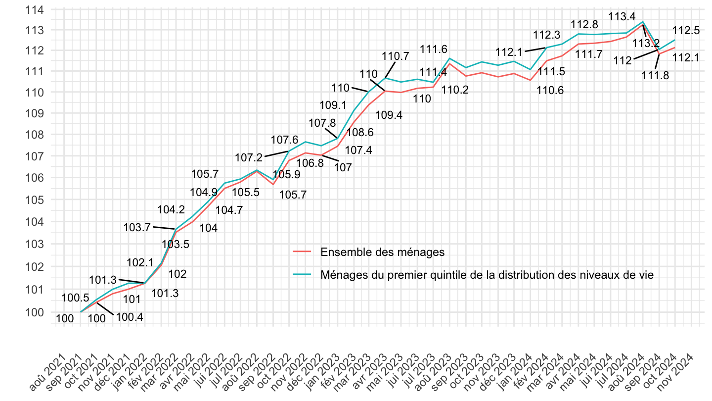
Cadres, Ouvriers, Retraités
Code
`IPC-2015` %>%
  filter(MENAGES_IPC %in% c("CADRE", "OUVRIER", "RETRAITE", "ACTIF")) %>%

  year_to_date %>%
  group_by(MENAGES_IPC) %>%
  arrange(date) %>%
  mutate(OBS_VALUE = 100*OBS_VALUE/OBS_VALUE[1]) %>%
  ggplot + geom_line(aes(x = date, y = OBS_VALUE, color = Menages_ipc)) +
  theme_minimal() + xlab("") + ylab("") +
  scale_x_date(breaks = seq(1920, 2100, 2) %>% paste0("-01-01") %>% as.Date,
               labels = date_format("%Y")) +
  theme(legend.position = c(0.7, 0.2),
        legend.title = element_blank()) +
  scale_y_log10(breaks = seq(0, 200, 5),
                     labels = dollar_format(accuracy = 1, prefix = "")) +
  geom_text_repel(data = . %>%
              filter(date == max(date)), aes(x = date, y = OBS_VALUE, label = round(OBS_VALUE, 1)), size = 3)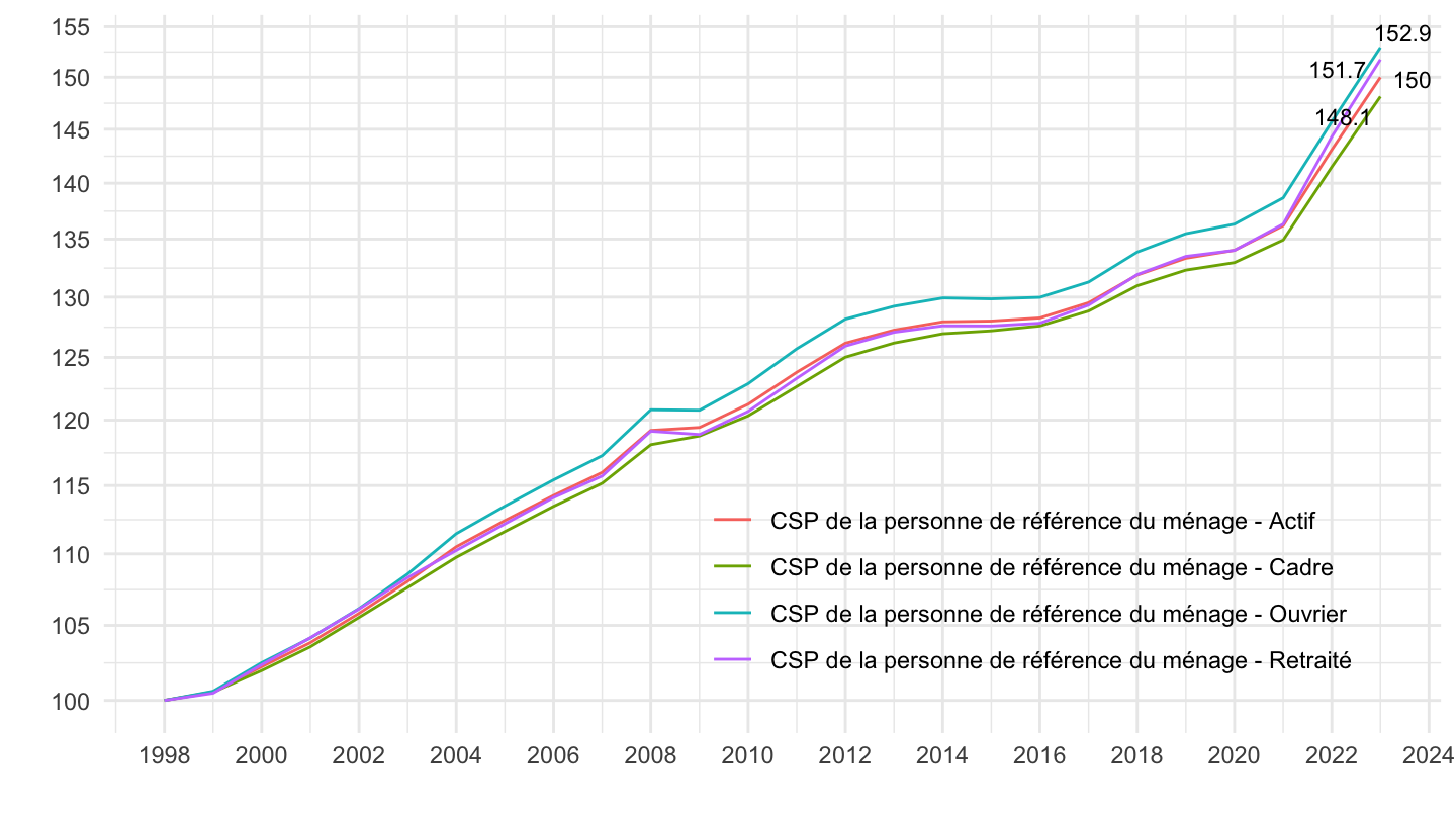
Inflation - Tous
Table - COICOP2016
All
Code
`IPC-2015` %>%
  filter(INDICATEUR == "IPC",
         MENAGES_IPC == "ENSEMBLE",
         REF_AREA == "FE",
         NATURE == "INDICE",
         PRIX_CONSO == "SO",
         TIME_PERIOD %in% c("1990", "2000", "2010", "2020")) %>%

  select(COICOP2016, Coicop2016, TIME_PERIOD, OBS_VALUE) %>%
  spread(TIME_PERIOD, OBS_VALUE) %>%
  mutate(`% 1990-2019` = (100*((`2020`/`1990`)^(1/29)-1)) %>% round(., 2)) %>%
  print_table_conditional
2-digit
Javascript
Code
`IPC-2015` %>%
  filter(INDICATEUR == "IPC",
         MENAGES_IPC == "ENSEMBLE",
         REF_AREA == "FE",
         NATURE == "INDICE",
         PRIX_CONSO == "SO",
         TIME_PERIOD %in% c("1990", "2000", "2010", "2020"),
         nchar(COICOP2016) == 2) %>%

  select(COICOP2016, Coicop2016, TIME_PERIOD, OBS_VALUE) %>%
  spread(TIME_PERIOD, OBS_VALUE) %>%
  mutate(`% 1990-2019` = (100*((`2020`/`1990`)^(1/29)-1)) %>% round(., 2)) %>%
print_table_conditional()| COICOP2016 | Coicop2016 | 1990 | 2000 | 2010 | 2020 | % 1990-2019 |
|---|---|---|---|---|---|---|
| 00 | 00 - Ensemble | 67.4 | 79.9 | 94.71 | 104.73 | 1.53 |
| 01 | 01 - Produits alimentaires et boissons non alcoolisées | 68.7 | 77.6 | 94.63 | 108.33 | 1.58 |
| 02 | 02 - Boissons alcoolisées, tabac et stupéfiants | 34.9 | 55.2 | 83.63 | 126.07 | 4.53 |
| 03 | 03 - Articles d'habillement et chaussures | 85.7 | 93.2 | 97.60 | 99.71 | 0.52 |
| 04 | 04 - Logement, eau, gaz, électricité et autres combustibles | 53.6 | 66.9 | 88.46 | 105.24 | 2.35 |
| 05 | 05 - Meubles, articles de ménage et entretien courant du foyer | 74.6 | 85.1 | 96.11 | 100.67 | 1.04 |
| 06 | 06 - Santé | 92.9 | 101.9 | 104.31 | 96.67 | 0.14 |
| 07 | 07 - Transports | 58.6 | 74.4 | 93.57 | 105.24 | 2.04 |
| 08 | 08 - Communications | 158.4 | 142.1 | 124.87 | 91.96 | -1.86 |
| 09 | 09 - Loisirs et culture | 101.5 | 109.2 | 101.30 | 103.29 | 0.06 |
| 10 | 10 - Enseignement | 55.3 | 70.0 | 92.09 | 107.42 | 2.32 |
| 11 | 11 - Restaurants et hôtels | 53.3 | 69.9 | 89.63 | 108.04 | 2.47 |
| 12 | 12 - Biens et services divers | 60.8 | 71.7 | 91.54 | 105.68 | 1.92 |
png
Code
i_g("bib/insee/IPC-2015_2digit.png")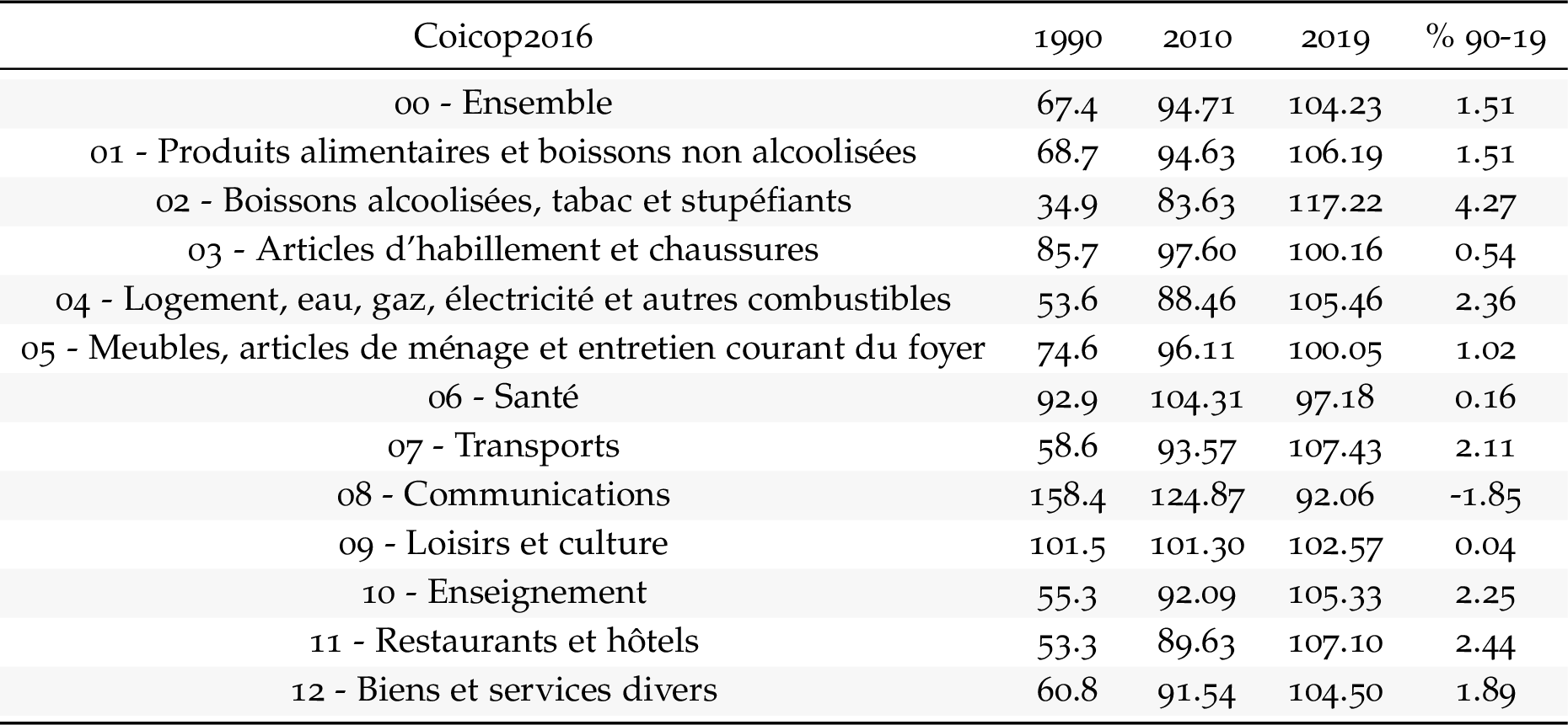
3-digit
Javascript
Code
`IPC-2015` %>%
  filter(INDICATEUR == "IPC",
         MENAGES_IPC == "ENSEMBLE",
         REF_AREA == "FE",
         NATURE == "INDICE",
         PRIX_CONSO == "SO",
         TIME_PERIOD %in% c("1990", "2000", "2010", "2020"),
         nchar(COICOP2016) == 3) %>%

  select(COICOP2016, Coicop2016, TIME_PERIOD, OBS_VALUE) %>%
  spread(TIME_PERIOD, OBS_VALUE) %>%
  mutate(`% 1990-2019` = (100*((`2020`/`1990`)^(1/29)-1)) %>% round(., 2)) %>%
  print_table_conditional()
png
Code
i_g("bib/insee/IPC-2015_3digit-0.png")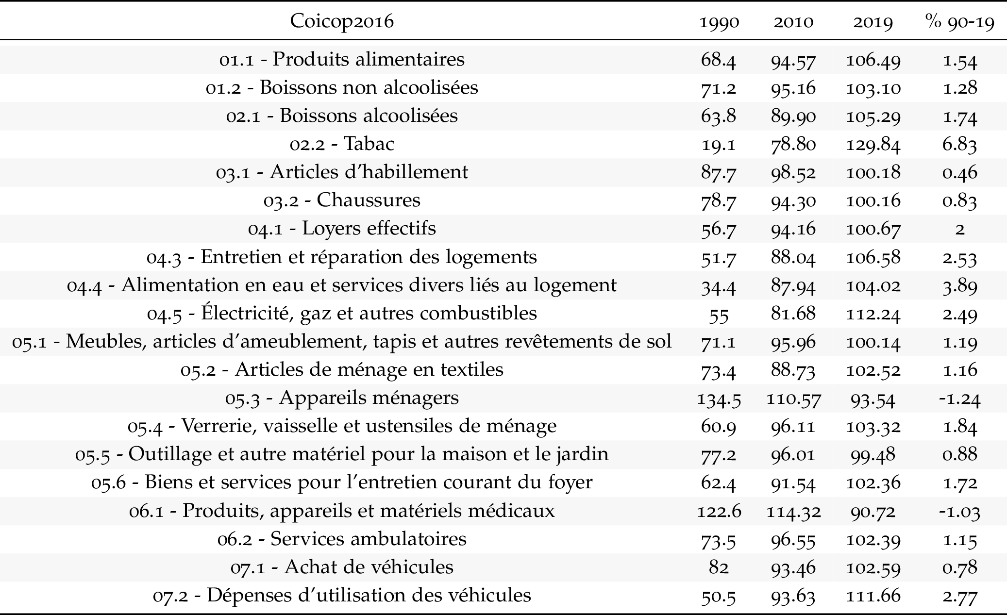
Code
i_g("bib/insee/IPC-2015_3digit-1.png")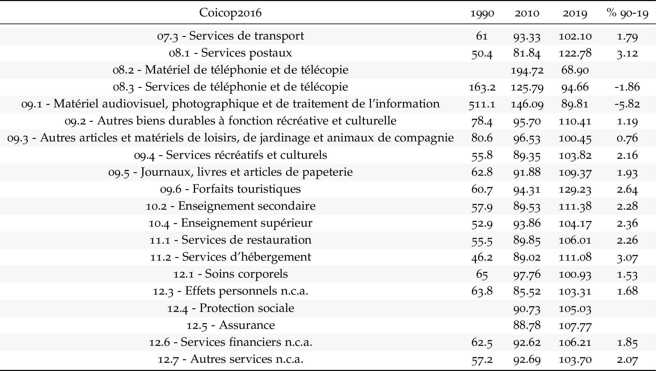
4-digit
Javascript
Code
`IPC-2015` %>%
  filter(INDICATEUR == "IPC",
         MENAGES_IPC == "ENSEMBLE",
         REF_AREA == "FE",
         NATURE == "INDICE",
         PRIX_CONSO == "SO",
         TIME_PERIOD %in% c("1990", "2000", "2010", "2020"),
         nchar(COICOP2016) == 4) %>%

  select(COICOP2016, Coicop2016, TIME_PERIOD, OBS_VALUE) %>%
  spread(TIME_PERIOD, OBS_VALUE) %>%
  mutate(`% 1990-2019` = (100*((`2020`/`1990`)^(1/29)-1)) %>% round(., 2)) %>%
  print_table_conditional()
png
Code
i_g("bib/insee/IPC-2015_4digit-0.png")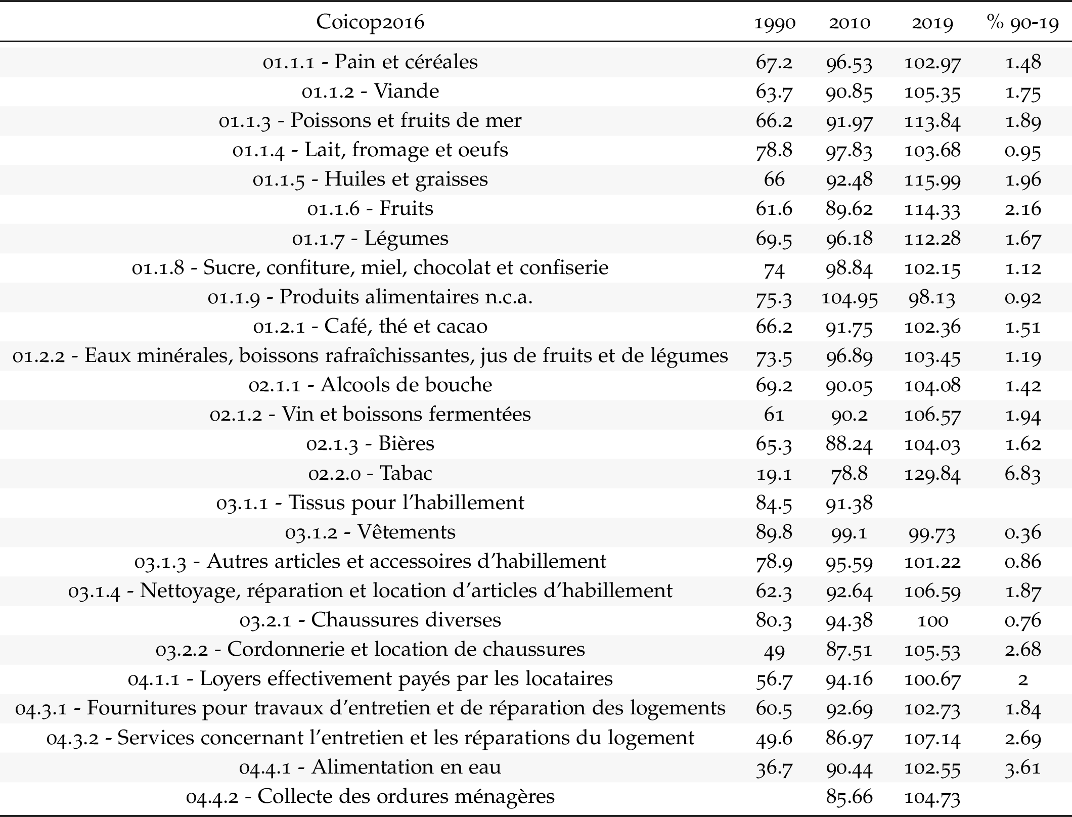
Code
i_g("bib/insee/IPC-2015_4digit-1.png")
Code
i_g("bib/insee/IPC-2015_4digit-2.png")
Code
i_g("bib/insee/IPC-2015_4digit-3.png")
5-digit
Code
`IPC-2015` %>%
  filter(INDICATEUR == "IPC",
         MENAGES_IPC == "ENSEMBLE",
         REF_AREA == "FE",
         NATURE == "INDICE",
         PRIX_CONSO == "SO",
         TIME_PERIOD %in% c("1990", "2000", "2010", "2020"),
         nchar(COICOP2016) == 5) %>%

  select(COICOP2016, Coicop2016, TIME_PERIOD, OBS_VALUE) %>%
  spread(TIME_PERIOD, OBS_VALUE) %>%
  mutate(`% 1990-2019` = (100*((`2020`/`1990`)^(1/29)-1)) %>% round(., 2)) %>%
  print_table_conditional()
6-digit
Code
`IPC-2015` %>%
  filter(INDICATEUR == "IPC",
         MENAGES_IPC == "ENSEMBLE",
         REF_AREA == "FE",
         NATURE == "INDICE",
         PRIX_CONSO == "SO",
         TIME_PERIOD %in% c("1990", "2000", "2010", "2020"),
         nchar(COICOP2016) == 6) %>%

  select(COICOP2016, Coicop2016, TIME_PERIOD, OBS_VALUE) %>%
  spread(TIME_PERIOD, OBS_VALUE) %>%
  mutate(`% 1990-2019` = (100*((`2020`/`1990`)^(1/29)-1)) %>% round(., 2)) %>%
  print_table_conditional()
Table - PRIX_CONSO
Code
`IPC-2015` %>%
  filter(INDICATEUR == "IPC",
         MENAGES_IPC == "ENSEMBLE",
         REF_AREA == "FE",
         NATURE == "INDICE",
         COICOP2016 == "SO",
         TIME_PERIOD %in% c("1990", "2000", "2010", "2020")) %>%


  select(PRIX_CONSO, Prix_conso, TIME_PERIOD, OBS_VALUE) %>%
  spread(TIME_PERIOD, OBS_VALUE) %>%
print_table_conditional| PRIX_CONSO | Prix_conso | 1990 | 2000 | 2010 | 2020 |
|---|---|---|---|---|---|
| 4000 | Alimentation | NA | NA | 94.14 | 108.10 |
| 4001 | Produits frais | NA | NA | 91.27 | 126.16 |
| 4002 | Autres produits alimentaires | NA | NA | 94.57 | 105.27 |
| 4003 | Produits manufacturés | NA | NA | 101.42 | 97.95 |
| 4004 | Habillement, chaussures | NA | NA | 97.80 | 99.42 |
| 4005 | Produits de santé | NA | NA | 114.95 | 88.35 |
| 4006 | Autres produits manufacturés | NA | NA | 99.31 | 99.98 |
| 4007 | Énergie | NA | NA | 88.98 | 108.34 |
| 4008 | Produits pétroliers | NA | NA | 97.83 | 106.18 |
| 4009 | Services | NA | NA | 92.90 | 105.22 |
| 4010 | Services : Loyers, eau et enlèvement des ordures ménagères | NA | NA | 92.41 | 101.88 |
| 4011 | Services : Services de santé | NA | NA | 96.55 | 102.75 |
| 4012 | Services : Transports et communications | NA | NA | 106.69 | 98.90 |
| 4013 | Autres services | NA | NA | 89.91 | 107.75 |
| 4014 | Alimentation, y compris tabac | NA | NA | 92.35 | 111.91 |
| 4015 | Produits manufacturés, y compris énergie | NA | NA | 98.65 | 100.37 |
| 4016 | Produits manufacturés, y compris services liés, hors habillement et chaussures | NA | NA | 102.07 | NA |
| 4017 | Ensemble hors énergie | NA | NA | 95.24 | 104.42 |
| 4018 | Ensemble hors tabac | NA | NA | 95.06 | 103.98 |
| 4023 | Ensemble hors tabac et alcool | NA | NA | 95.16 | 103.94 |
| 4024 | Ensemble non alimentaire, y compris tabac | NA | NA | 94.82 | 104.09 |
| 4025 | Ensemble hors produits frais | NA | NA | 94.80 | 104.26 |
| 4026 | Alimentation, y compris restaurants, cantines, cafés | NA | NA | 92.97 | 107.88 |
| 4037 | Biens durables | NA | NA | 102.00 | 99.95 |
| 4038 | Produits manufacturés, hors habillement, biens durables et produits de santé | NA | NA | 96.65 | 100.09 |
| 4566 | Services : Transports, communications, hôtellerie | NA | NA | 95.54 | 104.09 |
| 5000 | NA | NA | NA | 95.12 | 104.18 |
| 5272 | Services : Transports | 60.7 | 76.6 | 93.18 | 100.27 |
| 5273 | Services : Communications | 144.8 | 131.4 | 121.85 | 97.39 |
| 5329 | Produits manufacturés, hors habillement et chaussures | NA | NA | NA | 97.54 |
Inflation par catégorie
Tabac, Loyers, Ensemble, Carburants
Code
`IPC-2015` %>%
  filter(COICOP2016 %in% c("00", "045", "022", "0722"),
         NATURE == "INDICE",
         REF_AREA == "FE",
         FREQ == "M",
         is.na(MENAGES_IPC) | MENAGES_IPC == "ENSEMBLE",
         is.na(PRIX_CONSO) | PRIX_CONSO == "SO") %>%
  month_to_date %>%

  group_by(COICOP2016) %>%
  arrange(date) %>%
  mutate(OBS_VALUE = OBS_VALUE/lag(OBS_VALUE, 12)-1) %>%
  filter(date >= max(date) - years(2)) %>%
  select(date, OBS_VALUE, Coicop2016) %>%
  na.omit %>%
  ggplot() + ylab("Inflation sur un an (IPC, IPCH)") + xlab("") + theme_minimal() +
  geom_line(aes(x = date, y = OBS_VALUE, color = Coicop2016)) +

  scale_x_date(breaks = "1 month",
               labels = date_format("%b %Y")) +
  theme(legend.position = c(0.72, 0.9),
        legend.title = element_blank(),
        axis.text.x = element_text(angle = 45, vjust = 1, hjust = 1)) +
  scale_y_continuous(breaks = 0.01*seq(-100, 300, 5),
                     labels = percent_format(accuracy = 1, prefix = "")) +
  geom_text_repel(aes(x = date, y = OBS_VALUE, label = percent(OBS_VALUE, acc = 0.1)),
                  fontface ="plain", color = "black", size = 3)
Tabac, Loyers, Ensemble
Glissement 1 an
Code
`IPC-2015` %>%
  filter(COICOP2016 %in% c("00", "01", "022"),
         NATURE == "INDICE",
         REF_AREA == "FE",
         FREQ == "M",
         is.na(MENAGES_IPC) | MENAGES_IPC == "ENSEMBLE",
         is.na(PRIX_CONSO) | PRIX_CONSO == "SO") %>%
  month_to_date %>%

  group_by(COICOP2016) %>%
  arrange(date) %>%
  mutate(OBS_VALUE = OBS_VALUE/lag(OBS_VALUE, 12)-1) %>%
  filter(date >= max(date) - years(2)) %>%
  select(date, OBS_VALUE, Coicop2016) %>%
  na.omit %>%
  ggplot() + ylab("Inflation sur un an (IPC, IPCH)") + xlab("") + theme_minimal() +
  geom_line(aes(x = date, y = OBS_VALUE, color = Coicop2016)) +

  scale_x_date(breaks = "1 month",
               labels = date_format("%b %Y")) +
  theme(legend.position = c(0.3, 0.9),
        legend.title = element_blank(),
        axis.text.x = element_text(angle = 45, vjust = 1, hjust = 1)) +
  scale_y_continuous(breaks = 0.01*seq(-100, 300, 1),
                     labels = percent_format(accuracy = 1, prefix = "")) +
  geom_text_repel(aes(x = date, y = OBS_VALUE, label = percent(OBS_VALUE, acc = 0.1)),
                  fontface ="plain", color = "black", size = 3)
Glissement 2 ans
Code
`IPC-2015` %>%
  filter(COICOP2016 %in% c("00", "01", "022"),
         NATURE == "INDICE",
         REF_AREA == "FE",
         FREQ == "M",
         is.na(MENAGES_IPC) | MENAGES_IPC == "ENSEMBLE",
         is.na(PRIX_CONSO) | PRIX_CONSO == "SO") %>%
  month_to_date %>%

  group_by(COICOP2016) %>%
  arrange(date) %>%
  mutate(OBS_VALUE = OBS_VALUE/lag(OBS_VALUE, 24)-1) %>%
  filter(date >= max(date) - years(2)) %>%
  select(date, OBS_VALUE, Coicop2016) %>%
  na.omit %>%
  ggplot() + ylab("Glissement sur 2 ans (IPC, IPCH)") + xlab("") + theme_minimal() +
  geom_line(aes(x = date, y = OBS_VALUE, color = Coicop2016)) +

  scale_x_date(breaks = "1 month",
               labels = date_format("%b %Y")) +
  theme(legend.position = c(0.3, 0.9),
        legend.title = element_blank(),
        axis.text.x = element_text(angle = 45, vjust = 1, hjust = 1)) +
  scale_y_continuous(breaks = 0.01*seq(-100, 300, 1),
                     labels = percent_format(accuracy = 1, prefix = "")) +
  geom_text_repel(aes(x = date, y = OBS_VALUE, label = percent(OBS_VALUE, acc = 0.1)),
                  fontface ="plain", color = "black", size = 3)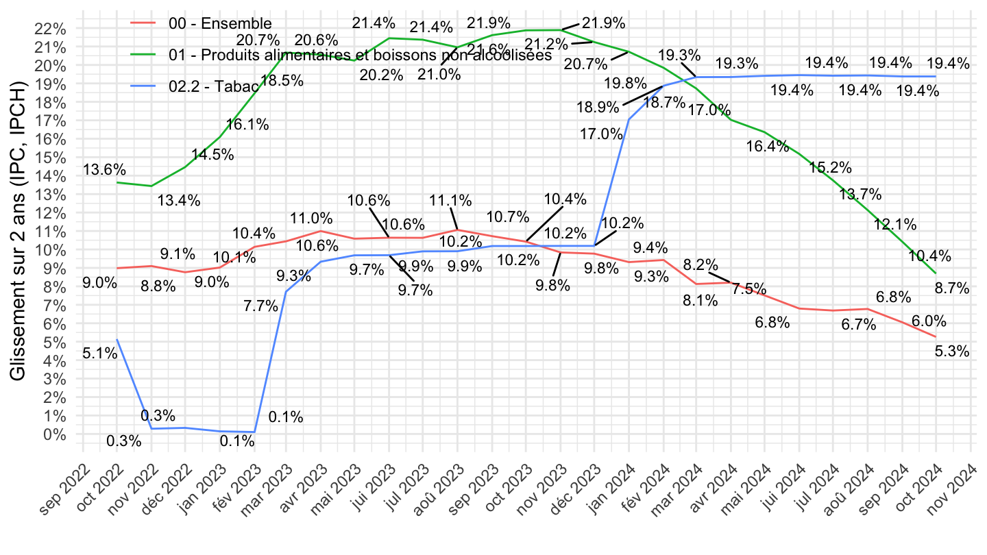
Alimentation, Loyers, Ensemble
Glissement 1 an
Code
`IPC-2015` %>%
  filter(COICOP2016 %in% c("00", "01", "041"),
         NATURE == "INDICE",
         REF_AREA == "FE",
         FREQ == "M",
         is.na(MENAGES_IPC) | MENAGES_IPC == "ENSEMBLE",
         is.na(PRIX_CONSO) | PRIX_CONSO == "SO") %>%
  month_to_date %>%

  group_by(COICOP2016) %>%
  arrange(date) %>%
  mutate(OBS_VALUE = OBS_VALUE/lag(OBS_VALUE, 12)-1) %>%
  filter(date >= max(date) - years(2)) %>%
  select(date, OBS_VALUE, Coicop2016) %>%
  na.omit %>%
  ggplot() + ylab("Glissement sur 1 an (IPC, IPCH)") + xlab("") + theme_minimal() +
  geom_line(aes(x = date, y = OBS_VALUE, color = Coicop2016)) +

  scale_x_date(breaks = "1 month",
               labels = date_format("%b %Y")) +
  theme(legend.position = c(0.3, 0.9),
        legend.title = element_blank(),
        axis.text.x = element_text(angle = 45, vjust = 1, hjust = 1)) +
  scale_y_continuous(breaks = 0.01*seq(-100, 300, 1),
                     labels = percent_format(accuracy = 1, prefix = "")) +
  geom_text_repel(aes(x = date, y = OBS_VALUE, label = percent(OBS_VALUE, acc = 0.1)),
                  fontface ="plain", color = "black", size = 3)
Glissement 2 ans
Code
`IPC-2015` %>%
  filter(COICOP2016 %in% c("00", "01", "041"),
         NATURE == "INDICE",
         REF_AREA == "FE",
         FREQ == "M",
         is.na(MENAGES_IPC) | MENAGES_IPC == "ENSEMBLE",
         is.na(PRIX_CONSO) | PRIX_CONSO == "SO") %>%
  month_to_date %>%

  group_by(COICOP2016) %>%
  arrange(date) %>%
  mutate(OBS_VALUE = OBS_VALUE/lag(OBS_VALUE, 24)-1) %>%
  filter(date >= max(date) - years(2)) %>%
  select(date, OBS_VALUE, Coicop2016) %>%
  na.omit %>%
  ggplot() + ylab("Glissement sur 2 ans (IPC, IPCH)") + xlab("") + theme_minimal() +
  geom_line(aes(x = date, y = OBS_VALUE, color = Coicop2016)) +

  scale_x_date(breaks = "1 month",
               labels = date_format("%b %Y")) +
  theme(legend.position = c(0.3, 0.9),
        legend.title = element_blank(),
        axis.text.x = element_text(angle = 45, vjust = 1, hjust = 1)) +
  scale_y_continuous(breaks = 0.01*seq(-100, 300, 1),
                     labels = percent_format(accuracy = 1, prefix = "")) +
  geom_text_repel(aes(x = date, y = OBS_VALUE, label = percent(OBS_VALUE, acc = 0.1)),
                  fontface ="plain", color = "black", size = 3)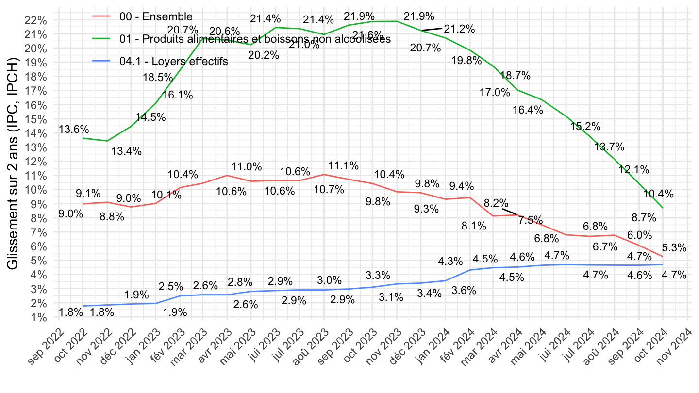
Chauffage du logement, Loyers, Ensemble
Glissement 1 an
Code
`IPC-2015` %>%
  filter(COICOP2016 %in% c("00", "041", "045"),
         NATURE == "INDICE",
         REF_AREA == "FE",
         FREQ == "M",
         is.na(MENAGES_IPC) | MENAGES_IPC == "ENSEMBLE",
         is.na(PRIX_CONSO) | PRIX_CONSO == "SO") %>%
  month_to_date %>%

  group_by(COICOP2016) %>%
  arrange(date) %>%
  mutate(OBS_VALUE = OBS_VALUE/lag(OBS_VALUE, 12)-1) %>%
  filter(date >= max(date) - years(2)) %>%
  select(date, OBS_VALUE, Coicop2016) %>%
  na.omit %>%
  ggplot() + ylab("Inflation sur un an (IPC, IPCH)") + xlab("") + theme_minimal() +
  geom_line(aes(x = date, y = OBS_VALUE, color = Coicop2016)) +

  scale_x_date(breaks = "1 month",
               labels = date_format("%b %Y")) +
  theme(legend.position = c(0.4, 0.45),
        legend.title = element_blank(),
        axis.text.x = element_text(angle = 45, vjust = 1, hjust = 1)) +
  scale_y_continuous(breaks = 0.01*seq(-100, 300, 2),
                     labels = percent_format(accuracy = 1, prefix = "")) +
  geom_text_repel(aes(x = date, y = OBS_VALUE, label = percent(OBS_VALUE, acc = 0.1)),
                  fontface ="plain", color = "black", size = 3)
Glissement 2 ans
Code
`IPC-2015` %>%
  filter(COICOP2016 %in% c("00", "041", "045"),
         NATURE == "INDICE",
         REF_AREA == "FE",
         FREQ == "M",
         is.na(MENAGES_IPC) | MENAGES_IPC == "ENSEMBLE",
         is.na(PRIX_CONSO) | PRIX_CONSO == "SO") %>%
  month_to_date %>%

  group_by(COICOP2016) %>%
  arrange(date) %>%
  mutate(OBS_VALUE = OBS_VALUE/lag(OBS_VALUE, 24)-1) %>%
  filter(date >= max(date) - years(2)) %>%
  select(date, OBS_VALUE, Coicop2016) %>%
  na.omit %>%
  ggplot() + ylab("Glissement sur 2 ans (IPC, IPCH)") + xlab("") + theme_minimal() +
  geom_line(aes(x = date, y = OBS_VALUE, color = Coicop2016)) +

  scale_x_date(breaks = "1 month",
               labels = date_format("%b %Y")) +
  theme(legend.position = c(0.4, 0.45),
        legend.title = element_blank(),
        axis.text.x = element_text(angle = 45, vjust = 1, hjust = 1)) +
  scale_y_continuous(breaks = 0.01*seq(-100, 300, 2),
                     labels = percent_format(accuracy = 1, prefix = "")) +
  geom_text_repel(aes(x = date, y = OBS_VALUE, label = percent(OBS_VALUE, acc = 0.1)),
                  fontface ="plain", color = "black", size = 3)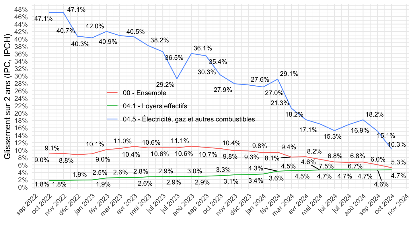
Pondérations d’indice
Table - COICOP2016
All
Code
`IPC-2015` %>%
  filter(INDICATEUR == "IPC",
         MENAGES_IPC == "ENSEMBLE",
         REF_AREA == "FE",
         NATURE == "POND",
         PRIX_CONSO == "SO",
         CORRECTION == "BRUT",
         TIME_PERIOD %in% c("1990", "2000", "2010", "2020")) %>%

  select(COICOP2016, Coicop2016, TIME_PERIOD, OBS_VALUE) %>%
  spread(TIME_PERIOD, OBS_VALUE) %>%
  print_table_conditional
2-digit
Javascript
Code
`IPC-2015` %>%
  filter(INDICATEUR == "IPC",
         MENAGES_IPC == "ENSEMBLE",
         REF_AREA == "FE",
         NATURE == "POND",
         PRIX_CONSO == "SO",
         TIME_PERIOD %in% c("1990", "2000", "2010", "2020"),
         nchar(COICOP2016) == 2) %>%

  select(COICOP2016, Coicop2016, TIME_PERIOD, OBS_VALUE) %>%
  spread(TIME_PERIOD, OBS_VALUE) %>%
print_table_conditional| COICOP2016 | Coicop2016 | 1990 | 2000 | 2010 | 2020 |
|---|---|---|---|---|---|
| 00 | 00 - Ensemble | 10000 | 10000 | 10000 | 10000 |
| 01 | 01 - Produits alimentaires et boissons non alcoolisées | 1999 | 1558 | 1474 | 1423 |
| 02 | 02 - Boissons alcoolisées, tabac et stupéfiants | 378 | 382 | 329 | 392 |
| 03 | 03 - Articles d'habillement et chaussures | 844 | 552 | 487 | 394 |
| 04 | 04 - Logement, eau, gaz, électricité et autres combustibles | 1233 | 1364 | 1348 | 1399 |
| 05 | 05 - Meubles, articles de ménage et entretien courant du foyer | 736 | 644 | 617 | 495 |
| 06 | 06 - Santé | 774 | 896 | 1005 | 1050 |
| 07 | 07 - Transports | 1659 | 1669 | 1634 | 1581 |
| 08 | 08 - Communications | 188 | 254 | 303 | 248 |
| 09 | 09 - Loisirs et culture | 851 | 859 | 916 | 854 |
| 10 | 10 - Enseignement | 33 | 23 | 25 | 5 |
| 11 | 11 - Restaurants et hôtels | 818 | 805 | 685 | 810 |
| 12 | 12 - Biens et services divers | 487 | 994 | 1177 | 1349 |
png
Code
i_g("bib/insee/IPC-2015_2digit_weights.png")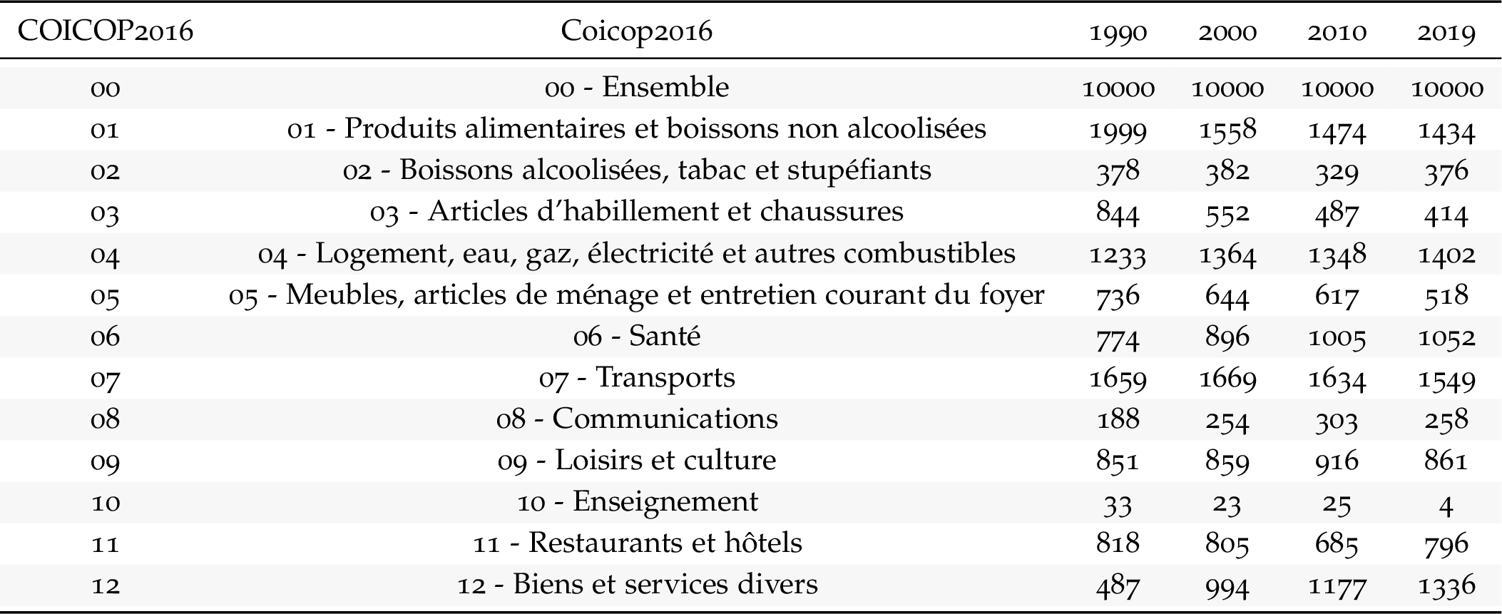
3-digit
Javascript
Code
`IPC-2015` %>%
  filter(INDICATEUR == "IPC",
         MENAGES_IPC == "ENSEMBLE",
         REF_AREA == "FE",
         NATURE == "POND",
         PRIX_CONSO == "SO",
         CORRECTION == "BRUT",
         TIME_PERIOD %in% c("1990", "2000", "2010", "2020"),
         nchar(COICOP2016) == 3) %>%

  select(COICOP2016, Coicop2016, TIME_PERIOD, OBS_VALUE) %>%
  spread(TIME_PERIOD, OBS_VALUE) %>%
  print_table_conditional
png
Code
i_g("bib/insee/IPC-2015_3digit_weights-0.png")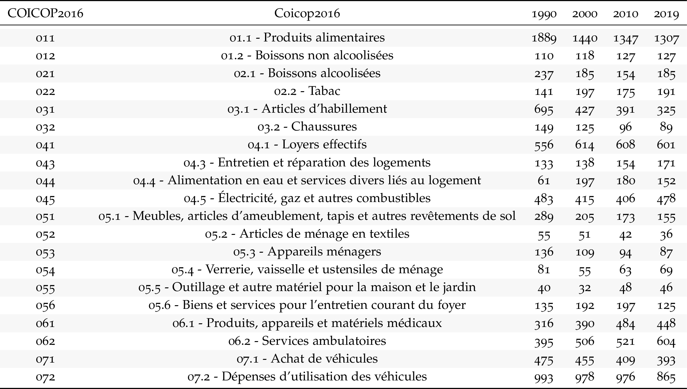
Code
i_g("bib/insee/IPC-2015_3digit_weights-1.png")
4-digit
Code
`IPC-2015` %>%
  filter(INDICATEUR == "IPC",
         MENAGES_IPC == "ENSEMBLE",
         REF_AREA == "FE",
         NATURE == "POND",
         PRIX_CONSO == "SO",
         CORRECTION == "BRUT",
         TIME_PERIOD %in% c("1990", "2000", "2010", "2020"),
         nchar(COICOP2016) == 4) %>%

  select(COICOP2016, Coicop2016, TIME_PERIOD, OBS_VALUE) %>%
  spread(TIME_PERIOD, OBS_VALUE) %>%
  print_table_conditional
5-digit
Code
`IPC-2015` %>%
  filter(INDICATEUR == "IPC",
         MENAGES_IPC == "ENSEMBLE",
         REF_AREA == "FE",
         NATURE == "POND",
         PRIX_CONSO == "SO",
         CORRECTION == "BRUT",
         TIME_PERIOD %in% c("1990", "2000", "2010", "2020"),
         nchar(COICOP2016) == 5) %>%

  select(COICOP2016, Coicop2016, TIME_PERIOD, OBS_VALUE) %>%
  spread(TIME_PERIOD, OBS_VALUE) %>%
  print_table_conditional
Table - PRIX_CONSO
1990, 2000, 2010, 2020
Code
`IPC-2015` %>%
  filter(INDICATEUR == "IPC",
         MENAGES_IPC == "ENSEMBLE",
         REF_AREA == "FE",
         NATURE == "POND",
         CORRECTION == "BRUT",
         COICOP2016 == "SO",
         TIME_PERIOD %in% c("1990", "2000", "2010", "2020")) %>%


  select(PRIX_CONSO, Prix_conso, TIME_PERIOD, OBS_VALUE) %>%
  spread(TIME_PERIOD, OBS_VALUE) %>%
  print_table_conditional
2016, 2017, 2018, 2019, 2020
Code
`IPC-2015` %>%
  filter(INDICATEUR == "IPC",
         MENAGES_IPC == "ENSEMBLE",
         REF_AREA == "FE",
         NATURE == "POND",
         CORRECTION == "BRUT",
         COICOP2016 == "SO",
         TIME_PERIOD %in% c("2016", "2017", "2018", "2019", "2020")) %>%


  select(PRIX_CONSO, Prix_conso, TIME_PERIOD, OBS_VALUE) %>%
  spread(TIME_PERIOD, OBS_VALUE) %>%
print_table_conditional()| PRIX_CONSO | Prix_conso | 2016 | 2017 | 2018 | 2019 | 2020 |
|---|---|---|---|---|---|---|
| 4000 | Alimentation | 1615 | 1627 | 1627 | 1619 | 1610 |
| 4001 | Produits frais | 217 | 235 | 243 | 244 | 230 |
| 4002 | Autres produits alimentaires | 1398 | 1392 | 1384 | 1375 | 1380 |
| 4003 | Produits manufacturés | 2651 | 2617 | 2594 | 2556 | 2491 |
| 4004 | Habillement, chaussures | 414 | 433 | 416 | 400 | 380 |
| 4005 | Produits de santé | 466 | 433 | 425 | 416 | 412 |
| 4006 | Autres produits manufacturés | 1771 | 1751 | 1753 | 1740 | 1699 |
| 4007 | Énergie | 773 | 748 | 777 | 804 | 808 |
| 4008 | Produits pétroliers | 419 | 378 | 408 | 425 | 439 |
| 4009 | Services | 4766 | 4820 | 4809 | 4830 | 4886 |
| 4010 | Services : Loyers, eau et enlèvement des ordures ménagères | 768 | 779 | 764 | 746 | 752 |
| 4011 | Services : Services de santé | 598 | 600 | 617 | 604 | 604 |
| 4012 | Services : Transports et communications | 524 | 524 | 505 | 504 | 515 |
| 4013 | Autres services | 2876 | 2917 | 2923 | 2976 | 3015 |
| 4014 | Alimentation, y compris tabac | 1810 | 1815 | 1820 | 1810 | 1815 |
| 4015 | Produits manufacturés, y compris énergie | 3434 | 3375 | 3382 | 3371 | 3311 |
| 4016 | Produits manufacturés, y compris services liés, hors habillement et chaussures | 2247 | 2194 | 2189 | 2167 | 2123 |
| 4017 | Ensemble hors énergie | 9227 | 9252 | 9223 | 9196 | 9192 |
| 4018 | Ensemble hors tabac | 9805 | 9812 | 9807 | 9809 | 9795 |
| 4024 | Ensemble non alimentaire, y compris tabac | 8385 | 8373 | 8373 | 8381 | 8390 |
| 4025 | Ensemble hors produits frais | 9798 | 9785 | 9776 | 9777 | 9790 |
| 4026 | Alimentation, y compris restaurants, cantines, cafés | 2185 | 2214 | 2229 | 2238 | 2239 |
| 4034 | Tabac | 195 | 188 | 193 | 191 | 205 |
| 4037 | Biens durables | 745 | 739 | 753 | 755 | 730 |
| 4038 | Produits manufacturés, hors habillement, biens durables et produits de santé | 1033 | 1019 | 1005 | 990 | 975 |
| 4566 | Services : Transports, communications, hôtellerie | 2304 | 2289 | 2359 | 2403 | 2440 |
| 5000 | NA | 9183 | 9183 | 9192 | 9208 | 9185 |
| 5272 | Services : Transports | 279 | 282 | 282 | 285 | 300 |
| 5273 | Services : Communications | 245 | 242 | 223 | 219 | 215 |
| 5329 | Produits manufacturés, hors habillement et chaussures | 2237 | 2184 | 2178 | 2156 | 2111 |
Alimentation, Produits alimentaires
Code
`IPC-2015` %>%
  filter(INDICATEUR == "IPC",
         MENAGES_IPC == "ENSEMBLE",
         COICOP2016 %in% c("01", "011"),
         REF_AREA == "FE",
         NATURE == "POND") %>%
  year_to_date %>%

  mutate(OBS_VALUE = OBS_VALUE/10000) %>%
  ggplot() + ylab("Poids de l'alimentation dans l'indice des prix") + xlab("") + theme_minimal() +
  geom_line(aes(x = date, y = OBS_VALUE, color = Coicop2016)) +
  scale_x_date(breaks = seq(1920, 2100, 5) %>% paste0("-01-01") %>% as.Date,
               labels = date_format("%Y")) +
  theme(legend.position = c(0.65, 0.9),
        legend.title = element_blank()) +
  scale_y_continuous(breaks = 0.01*seq(0, 40, 0.5),
                     labels = percent_format(accuracy = .1))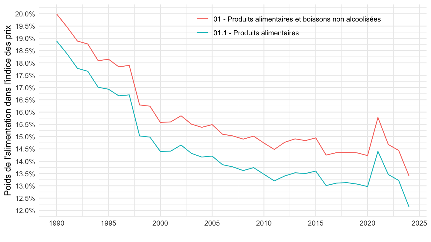
Tabac
Code
`IPC-2015` %>%
  filter(INDICATEUR == "IPC",
         MENAGES_IPC == "ENSEMBLE",
         COICOP2016 %in% c("022"),
         REF_AREA == "FE",
         NATURE == "POND") %>%
  year_to_date %>%

  mutate(OBS_VALUE = OBS_VALUE/10000) %>%
  ggplot() + ylab("Poids du tabac dans l'indice des prix") + xlab("") + theme_minimal() +
  geom_line(aes(x = date, y = OBS_VALUE)) +

  scale_x_date(breaks = seq(1920, 2100, 5) %>% paste0("-01-01") %>% as.Date,
               labels = date_format("%Y")) +
  scale_y_continuous(breaks = 0.01*seq(0, 10, 0.1),
                     labels = percent_format(accuracy = .1))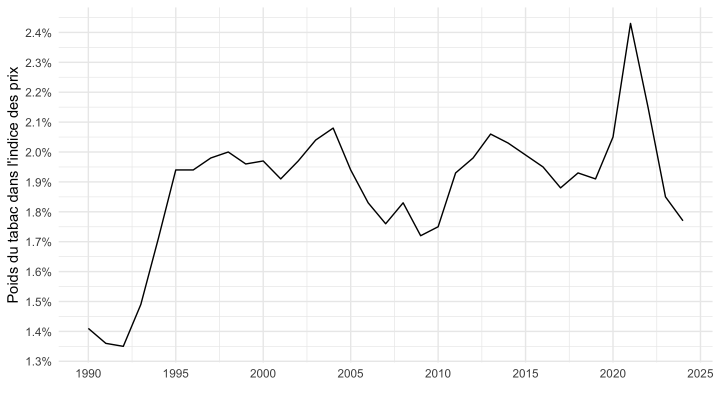
0943 - Jeux de hasard (en pratique: tickets de lotterie)
Tous
Code
`IPC-2015` %>%
  filter(INDICATEUR == "IPC",
         MENAGES_IPC == "ENSEMBLE",
         COICOP2016 %in% c("0943"),
         REF_AREA == "FE",
         NATURE == "POND") %>%
  year_to_date %>%

  mutate(OBS_VALUE = OBS_VALUE/10000) %>%
  ggplot() + ylab("Poids des jeux de hasard dans l'IPC") + xlab("") + theme_minimal() +
  geom_line(aes(x = date, y = OBS_VALUE)) +

  scale_x_date(breaks = seq(1920, 2100, 1) %>% paste0("-01-01") %>% as.Date,
               labels = date_format("%Y")) +
  theme(legend.position = c(0.15, 0.9),
        legend.title = element_blank()) +
  scale_y_continuous(breaks = 0.01*seq(0, 10, 0.02),
                     labels = percent_format(accuracy = .01))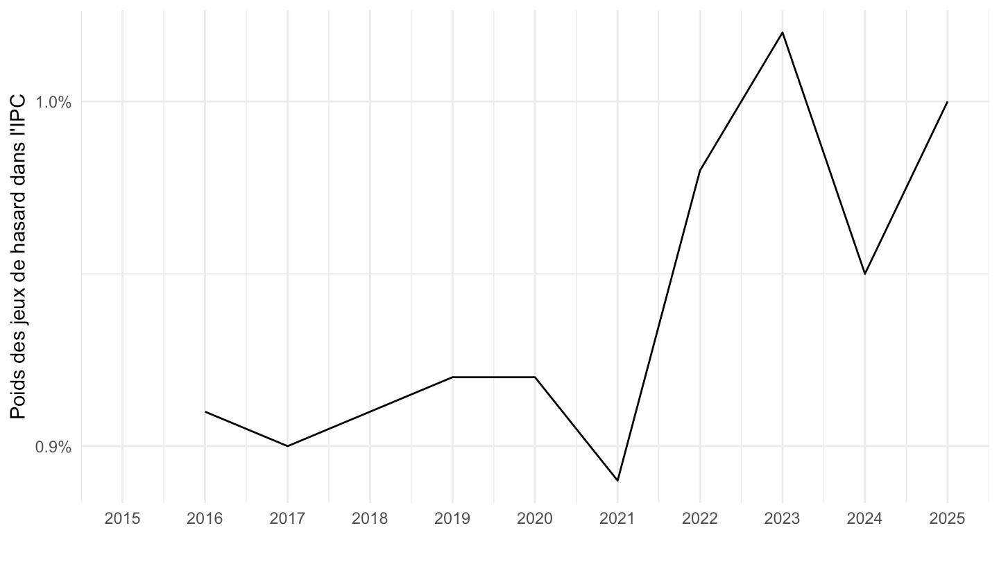
-2024
Code
`IPC-2015` %>%
  filter(INDICATEUR == "IPC",
         MENAGES_IPC == "ENSEMBLE",
         COICOP2016 %in% c("0943"),
         REF_AREA == "FE",
         NATURE == "POND") %>%
  year_to_date %>%

  mutate(OBS_VALUE = OBS_VALUE/10000) %>%
  filter(date <= as.Date("2024-01-01")) %>%
  ggplot() + ylab("Poids des jeux de hasard dans l'IPC") + xlab("") + theme_minimal() +
  geom_line(aes(x = date, y = OBS_VALUE)) +

  scale_x_date(breaks = seq(1920, 2100, 1) %>% paste0("-01-01") %>% as.Date,
               labels = date_format("%Y")) +
  theme(legend.position = c(0.15, 0.9),
        legend.title = element_blank()) +
  scale_y_continuous(breaks = 0.01*seq(0, 10, 0.02),
                     labels = percent_format(accuracy = .01))
1253 - Assurance Santé Complémentaire
Code
`IPC-2015` %>%
  filter(INDICATEUR == "IPC",
         MENAGES_IPC == "ENSEMBLE",
         COICOP2016 %in% c("1253"),
         REF_AREA == "FE",
         NATURE == "POND") %>%
  year_to_date %>%

  mutate(OBS_VALUE = OBS_VALUE/10000) %>%
  ggplot() + ylab("Poids de l'assurance santé dans l'indice des prix") + xlab("") + theme_minimal() +
  geom_line(aes(x = date, y = OBS_VALUE)) +

  scale_x_date(breaks = seq(1920, 2100, 2) %>% paste0("-01-01") %>% as.Date,
               labels = date_format("%Y")) +
  theme(legend.position = c(0.15, 0.9),
        legend.title = element_blank()) +
  scale_y_continuous(breaks = 0.01*seq(0, 10, 0.1),
                     labels = percent_format(accuracy = .1))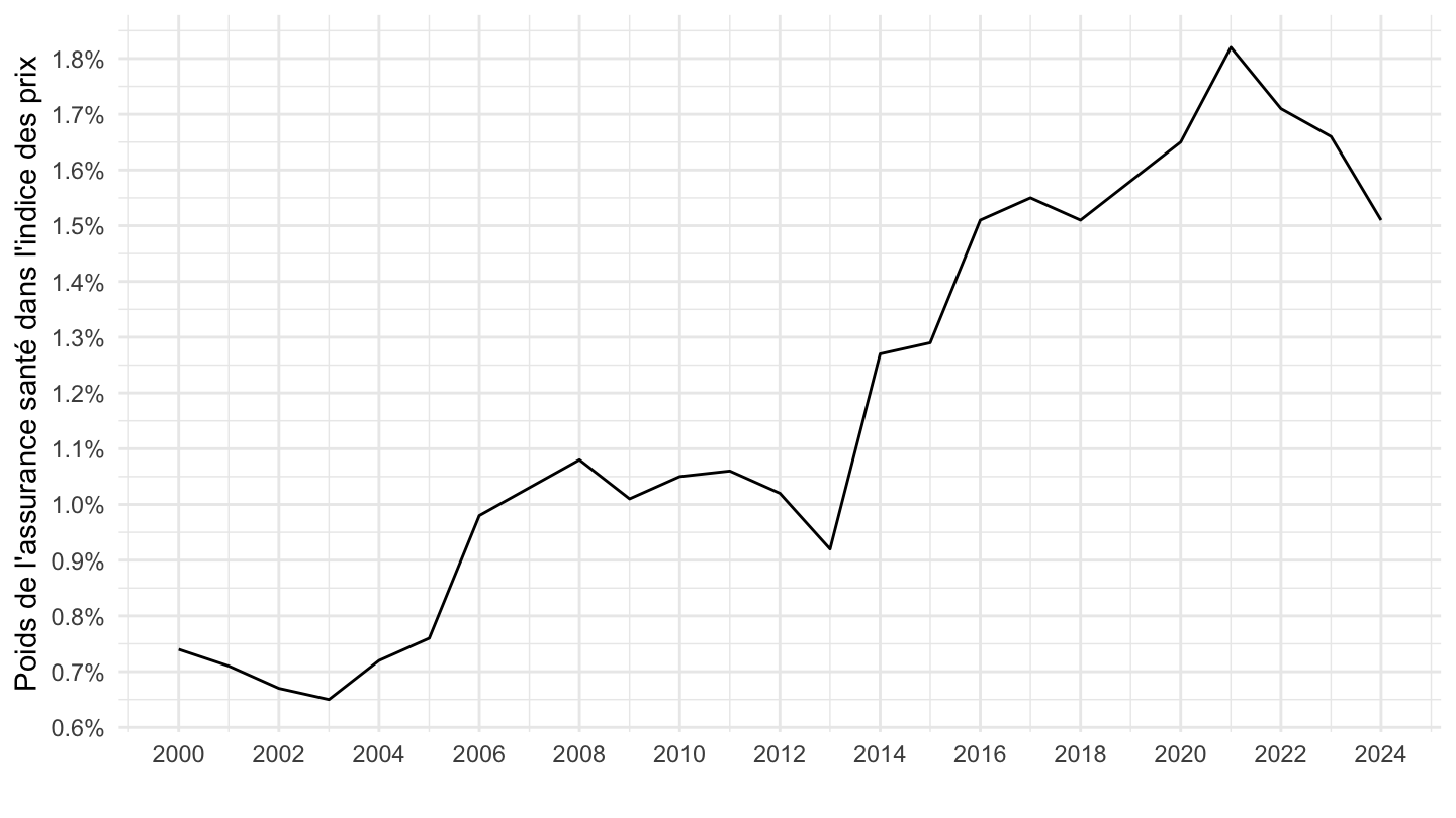
Santé
Code
`IPC-2015` %>%
  filter(INDICATEUR == "IPC",
         MENAGES_IPC == "ENSEMBLE",
         COICOP2016 %in% c("06"),
         REF_AREA == "FE",
         NATURE == "POND") %>%
  year_to_date %>%

  mutate(OBS_VALUE = OBS_VALUE/10000) %>%
  ggplot() + ylab("Poids de la santé dans l'indice des prix") + xlab("") + theme_minimal() +
  geom_line(aes(x = date, y = OBS_VALUE)) +

  scale_x_date(breaks = seq(1920, 2100, 5) %>% paste0("-01-01") %>% as.Date,
               labels = date_format("%Y")) +
  scale_y_continuous(breaks = 0.01*seq(0, 20, 0.5),
                     labels = percent_format(accuracy = .1))
Logement total
Code
`IPC-2015` %>%
  filter(INDICATEUR == "IPC",
         MENAGES_IPC == "ENSEMBLE",
         COICOP2016 %in% c("04", "041"),
         REF_AREA == "FE",
         NATURE == "POND") %>%
  year_to_date %>%

  mutate(OBS_VALUE = OBS_VALUE/10000) %>%
  ggplot() + ylab("Poids du logement dans l'indice des prix IPC") + xlab("") + theme_minimal() +
  geom_line(aes(x = date, y = OBS_VALUE, color = Coicop2016)) +

  scale_x_date(breaks = seq(1920, 2100, 5) %>% paste0("-01-01") %>% as.Date,
               labels = date_format("%Y")) +
  theme(legend.position = c(0.4, 0.9),
        legend.title = element_blank()) +
  scale_y_continuous(breaks = 0.01*seq(0, 20, 0.5),
                     labels = percent_format(accuracy = .1))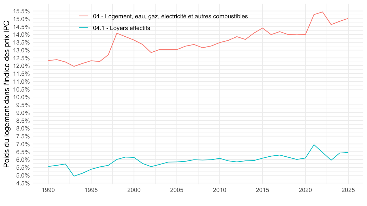
Santé, Assurance santé complémentaire
All
Code
`IPC-2015` %>%
  filter(INDICATEUR == "IPC",
         MENAGES_IPC == "ENSEMBLE",
         COICOP2016 %in% c("06", "1253"),
         REF_AREA == "FE",
         NATURE == "POND") %>%
  year_to_date %>%

  mutate(OBS_VALUE = OBS_VALUE/10000) %>%
  ggplot() + ylab("Poids de la santé dans l'indice des prix") + xlab("") + theme_minimal() +
  geom_line(aes(x = date, y = OBS_VALUE, color = Coicop2016)) +
  scale_color_manual(values = viridis(2)[1:2]) +
  scale_x_date(breaks = seq(1920, 2100, 2) %>% paste0("-01-01") %>% as.Date,
               labels = date_format("%Y")) +
  theme(legend.position = c(0.15, 0.9),
        legend.title = element_blank()) +
  scale_y_continuous(breaks = 0.01*seq(0, 20, 0.5),
                     labels = percent_format(accuracy = .1))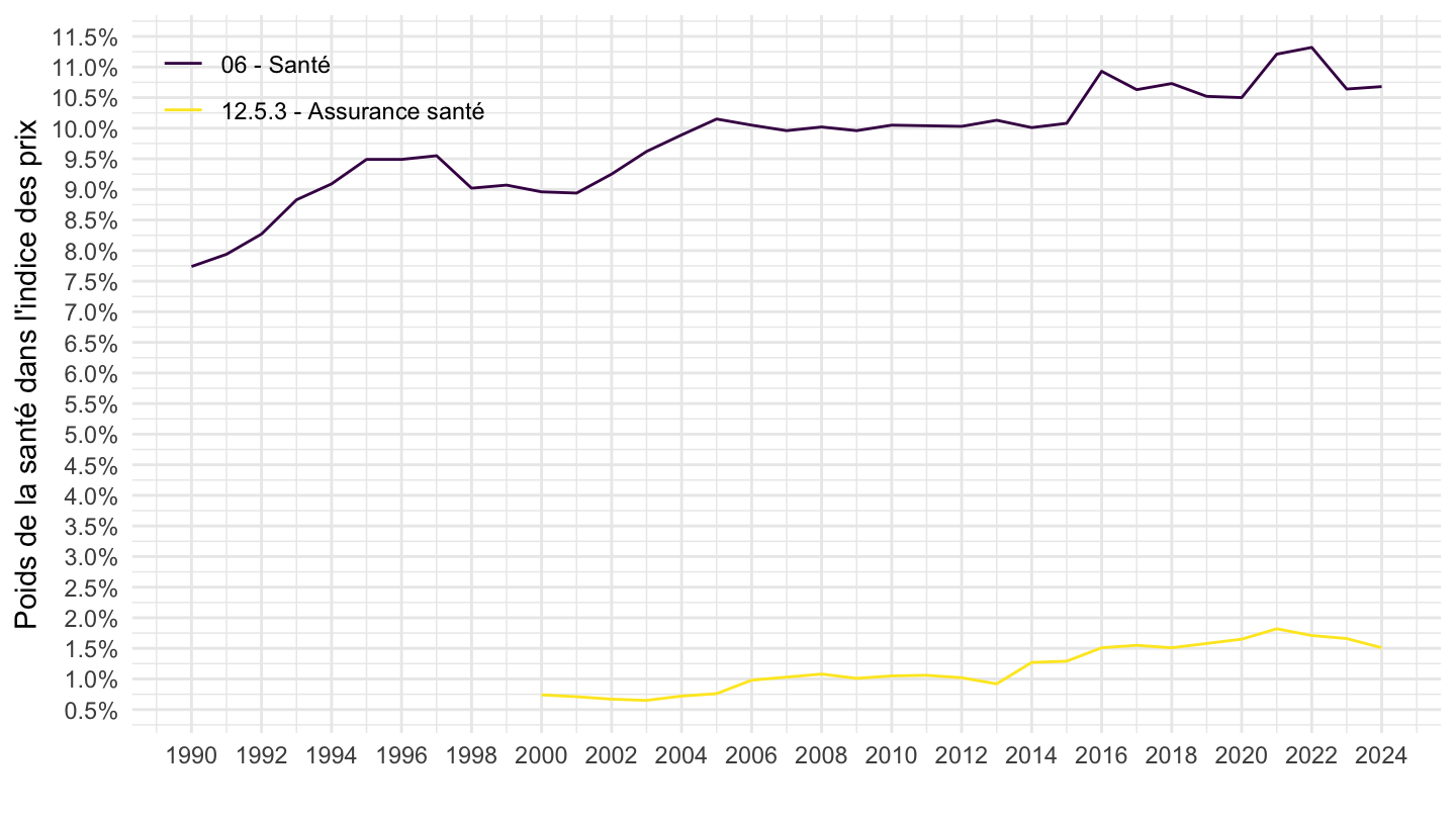
1996-
Code
`IPC-2015` %>%
  filter(INDICATEUR == "IPC",
         MENAGES_IPC == "ENSEMBLE",
         COICOP2016 %in% c("06", "1253"),
         REF_AREA == "FE",
         NATURE == "POND") %>%
  year_to_date %>%
  filter(date >= as.Date("1996-01-01")) %>%

  mutate(OBS_VALUE = OBS_VALUE/10000) %>%
  ggplot() + ylab("Poids de la santé dans l'indice des prix") + xlab("") + theme_minimal() +
  geom_line(aes(x = date, y = OBS_VALUE, color = Coicop2016)) +
  scale_color_manual(values = viridis(2)[1:2]) +
  scale_x_date(breaks = seq(1920, 2100, 2) %>% paste0("-01-01") %>% as.Date,
               labels = date_format("%Y")) +
  theme(legend.position = c(0.15, 0.9),
        legend.title = element_blank()) +
  scale_y_continuous(breaks = 0.01*seq(0, 20, 0.5),
                     labels = percent_format(accuracy = .1))
Santé
Santé, Assurance Santé vs. Ensemble
1990-
Code
`IPC-2015` %>%
  filter(INDICATEUR == "IPC",
         MENAGES_IPC == "ENSEMBLE",
         PRIX_CONSO == "SO",
         COICOP2016 %in% c("06", "1253", "00"),
         FREQ == "M",
         REF_AREA == "FE",
         NATURE == "INDICE") %>%
  month_to_date %>%

  group_by(Coicop2016) %>%
  arrange(date) %>%
  mutate(OBS_VALUE = 100*OBS_VALUE/OBS_VALUE[1]) %>%
  ggplot() + ylab("Indice des prix") + xlab("") + theme_minimal() +
  geom_line(aes(x = date, y = OBS_VALUE, color = Coicop2016)) +

  scale_x_date(breaks = seq(1920, 2100, 5) %>% paste0("-01-01") %>% as.Date,
               labels = date_format("%Y")) +
  theme(legend.position = c(0.15, 0.9),
        legend.title = element_blank()) +
  scale_y_log10(breaks = c(100, 164, 200, 400, 816, seq(100, 180, 10)),
                     labels = dollar_format(accuracy = 1, prefix = ""))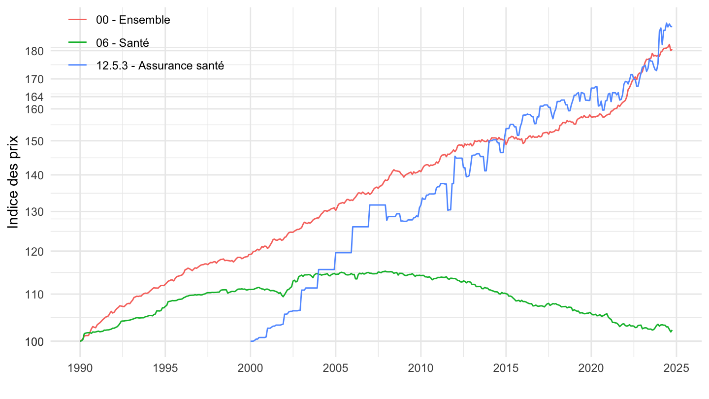
1996-
Code
`IPC-2015` %>%
  filter(INDICATEUR == "IPC",
         MENAGES_IPC == "ENSEMBLE",
         PRIX_CONSO == "SO",
         COICOP2016 %in% c("06", "1253", "00"),
         FREQ == "M",
         REF_AREA == "FE",
         NATURE == "INDICE") %>%
  month_to_date %>%
  filter(date >= as.Date("1996-01-01")) %>%

  group_by(Coicop2016) %>%
  arrange(date) %>%
  mutate(OBS_VALUE = 100*OBS_VALUE/OBS_VALUE[1]) %>%
  ggplot() + ylab("Indice des prix, IPC") + xlab("") + theme_minimal() +
  geom_line(aes(x = date, y = OBS_VALUE, color = Coicop2016)) +

  scale_x_date(breaks = seq(1920, 2100, 2) %>% paste0("-01-01") %>% as.Date,
               labels = date_format("%Y")) +
  theme(legend.position = c(0.15, 0.9),
        legend.title = element_blank()) +
  scale_y_log10(breaks = c(100, 164, 200, 400, 816, seq(100, 180, 10)),
                     labels = dollar_format(accuracy = 1, prefix = ""))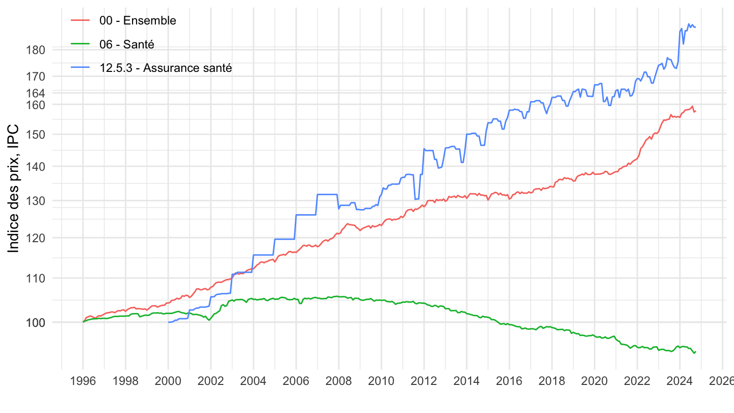
Péages
Péages vs. Ensemble
1990-
Code
`IPC-2015` %>%
  filter(INDICATEUR == "IPC",
         MENAGES_IPC == "ENSEMBLE",
         PRIX_CONSO == "SO",
         COICOP2016 %in% c("07242", "0724", "00"),
         FREQ == "M",
         REF_AREA == "FE",
         NATURE == "INDICE") %>%
  month_to_date %>%

  group_by(Coicop2016) %>%
  arrange(date) %>%
  mutate(OBS_VALUE = 100*OBS_VALUE/OBS_VALUE[1]) %>%
  ggplot() + ylab("Indice des prix") + xlab("") + theme_minimal() +
  geom_line(aes(x = date, y = OBS_VALUE, color = Coicop2016)) +

  scale_x_date(breaks = seq(1920, 2100, 5) %>% paste0("-01-01") %>% as.Date,
               labels = date_format("%Y")) +
  theme(legend.position = c(0.35, 0.9),
        legend.title = element_blank()) +
  scale_y_log10(breaks = seq(100, 400, 10),
                     labels = dollar_format(accuracy = 1, prefix = ""))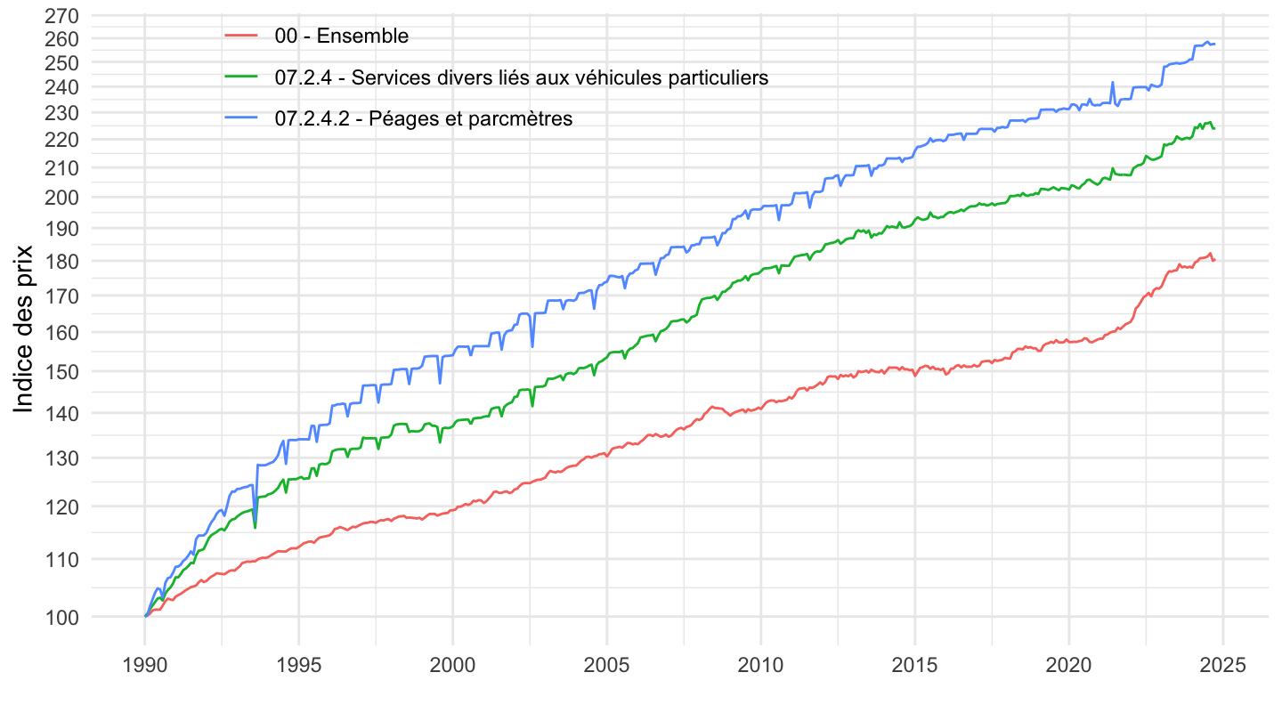
1996-
Code
`IPC-2015` %>%
  filter(INDICATEUR == "IPC",
         MENAGES_IPC == "ENSEMBLE",
         PRIX_CONSO == "SO",
         COICOP2016 %in% c("07242", "0724", "00"),
         FREQ == "M",
         REF_AREA == "FE",
         NATURE == "INDICE") %>%
  month_to_date %>%

  filter(date >= as.Date("1996-01-01")) %>%
  group_by(Coicop2016) %>%
  arrange(date) %>%
  mutate(OBS_VALUE = 100*OBS_VALUE/OBS_VALUE[1]) %>%
  ggplot() + ylab("Indice des prix") + xlab("") + theme_minimal() +
  geom_line(aes(x = date, y = OBS_VALUE, color = Coicop2016)) +

  scale_x_date(breaks = seq(1920, 2100, 2) %>% paste0("-01-01") %>% as.Date,
               labels = date_format("%Y")) +
  theme(legend.position = c(0.35, 0.9),
        legend.title = element_blank()) +
  scale_y_log10(breaks = seq(100, 400, 10),
                     labels = dollar_format(accuracy = 1, prefix = ""))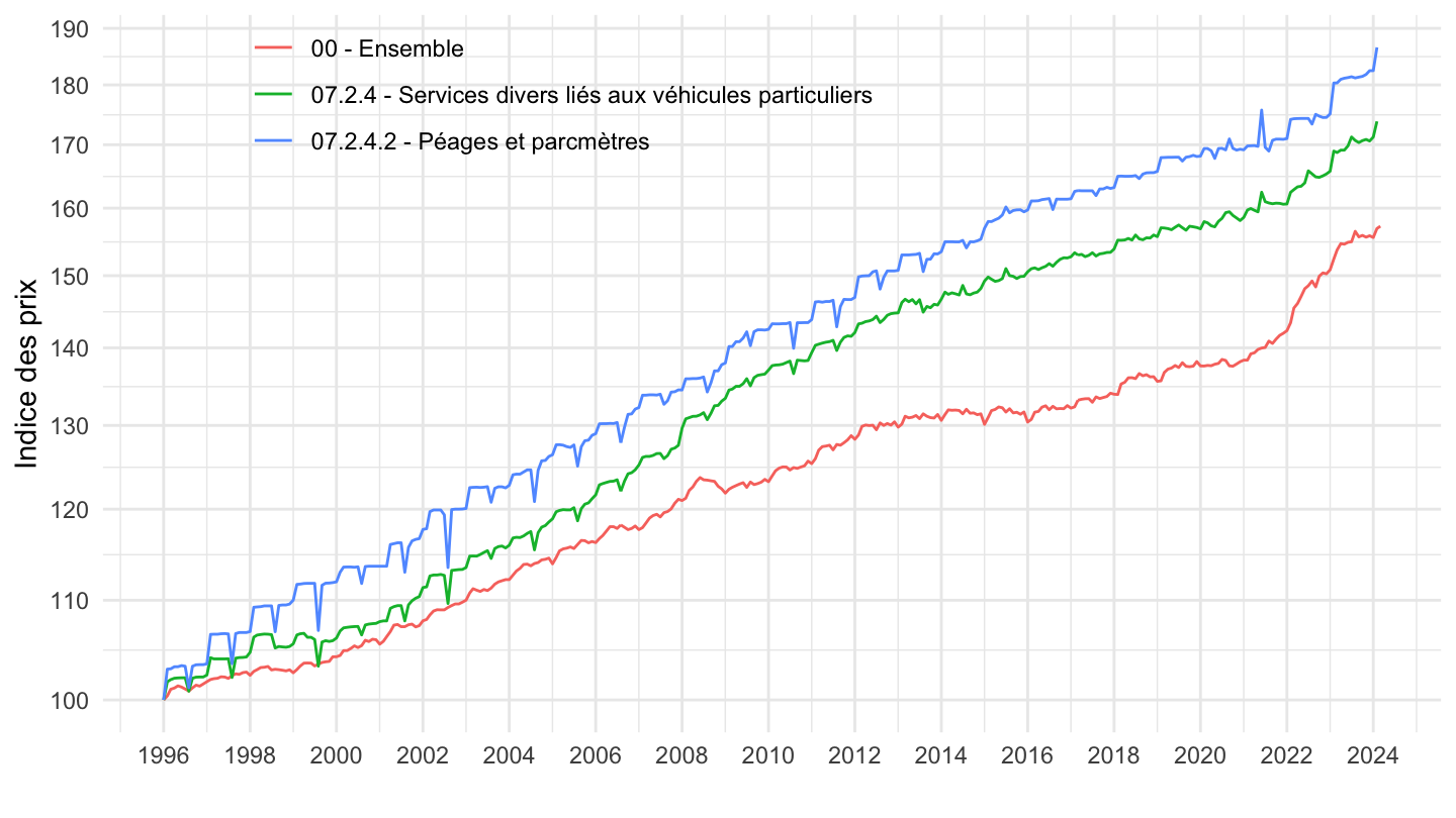
Pondération des péages, services divers dans l’IPC
1990-
Code
`IPC-2015` %>%
  filter(INDICATEUR == "IPC",
         MENAGES_IPC == "ENSEMBLE",
         COICOP2016 %in% c("07242", "0724"),
         REF_AREA == "FE",
         NATURE == "POND") %>%
  year_to_date %>%

  mutate(OBS_VALUE = OBS_VALUE/10000) %>%
  ggplot() + ylab("Poids des péages dans l'indice des prix") + xlab("") + theme_minimal() +
  geom_line(aes(x = date, y = OBS_VALUE, color = Coicop2016)) +

  theme(legend.position = c(0.35, 0.9),
        legend.title = element_blank()) +
  scale_x_date(breaks = seq(1920, 2100, 5) %>% paste0("-01-01") %>% as.Date,
               labels = date_format("%Y")) +
  scale_y_continuous(breaks = 0.01*seq(0, 10, 0.1),
                     labels = percent_format(accuracy = .1),
                     limits = c(0, 0.016))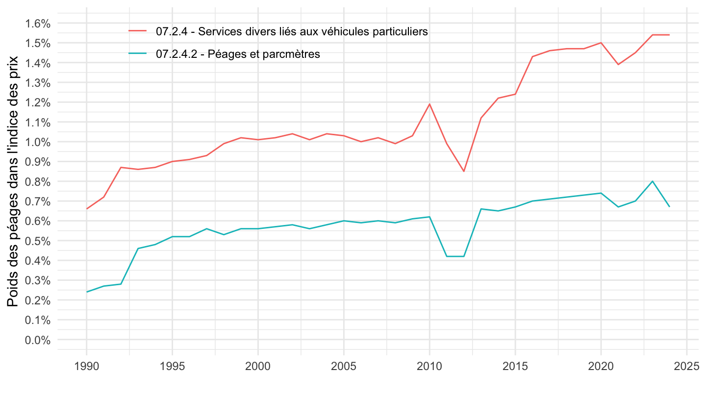
1996-
Code
`IPC-2015` %>%
  filter(INDICATEUR == "IPC",
         MENAGES_IPC == "ENSEMBLE",
         COICOP2016 %in% c("07242", "0724"),
         REF_AREA == "FE",
         NATURE == "POND") %>%
  year_to_date %>%

  mutate(OBS_VALUE = OBS_VALUE/10000) %>%
  filter(date >= as.Date("1996-01-01")) %>%
  ggplot() + ylab("Poids des péages dans l'indice des prix") + xlab("") + theme_minimal() +
  geom_line(aes(x = date, y = OBS_VALUE, color = Coicop2016)) +

  theme(legend.position = c(0.35, 0.9),
        legend.title = element_blank()) +
  scale_x_date(breaks = seq(1920, 2100, 2) %>% paste0("-01-01") %>% as.Date,
               labels = date_format("%Y")) +
  scale_y_continuous(breaks = 0.01*seq(0, 10, 0.1),
                     labels = percent_format(accuracy = .1),
                     limits = c(0, 0.016))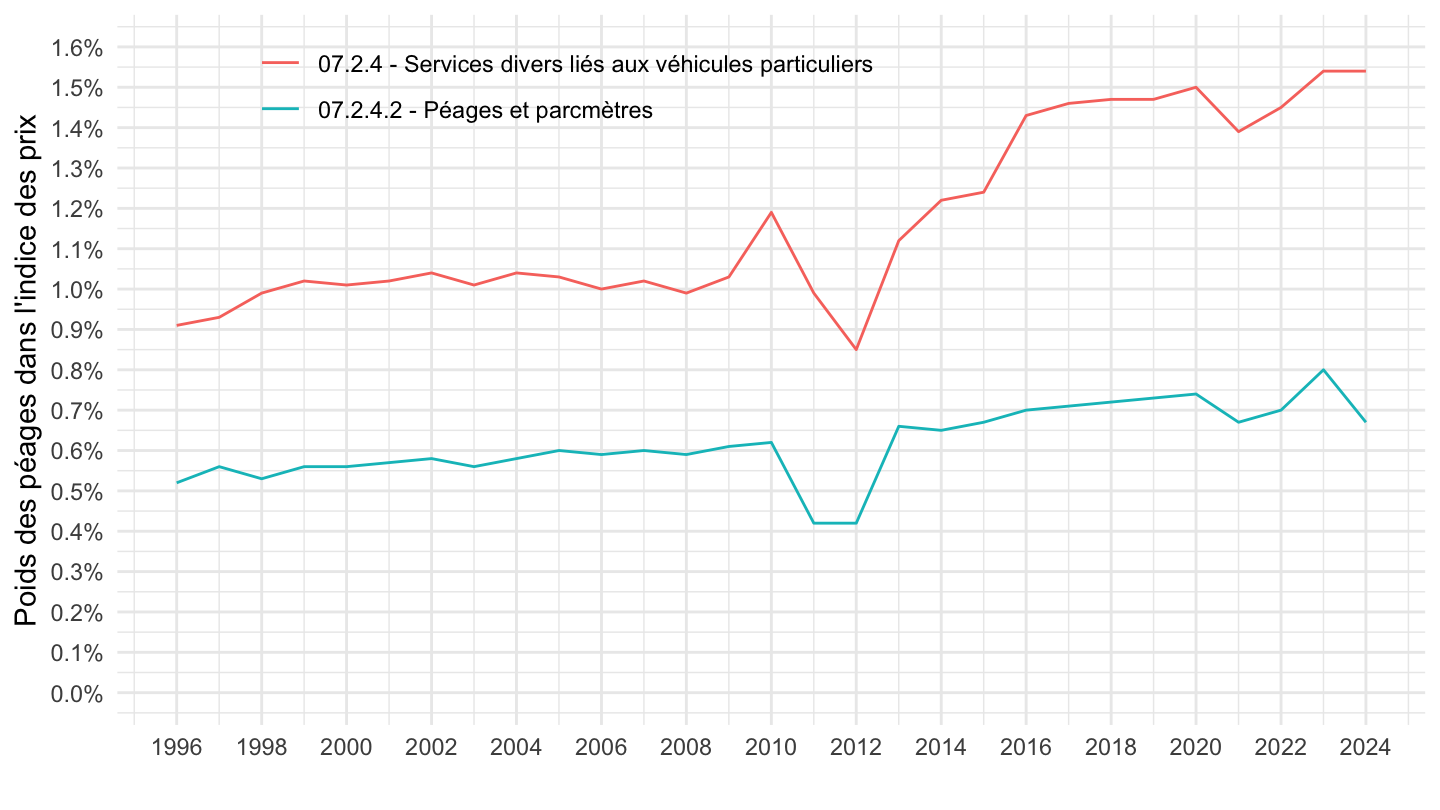
Services à domicile
Services à domicile vs. Ensemble
1998-
Code
`IPC-2015` %>%
  filter(INDICATEUR == "IPC",
         MENAGES_IPC == "ENSEMBLE",
         PRIX_CONSO == "SO",
         COICOP2016 %in% c("05621", "00"),
         FREQ == "M",
         REF_AREA == "FE",
         NATURE == "INDICE") %>%
  month_to_date %>%
  filter(date >= as.Date("1998-01-01")) %>%

  group_by(Coicop2016) %>%
  arrange(date) %>%
  mutate(OBS_VALUE = 100*OBS_VALUE/OBS_VALUE[1]) %>%
  ggplot() + ylab("Indice des prix") + xlab("") + theme_minimal() +
  geom_line(aes(x = date, y = OBS_VALUE, color = Coicop2016)) +

  scale_x_date(breaks = seq(1920, 2100, 2) %>% paste0("-01-01") %>% as.Date,
               labels = date_format("%Y")) +
  theme(legend.position = c(0.35, 0.9),
        legend.title = element_blank()) +
  scale_y_log10(breaks = seq(100, 200, 10),
                     labels = dollar_format(accuracy = 1, prefix = ""))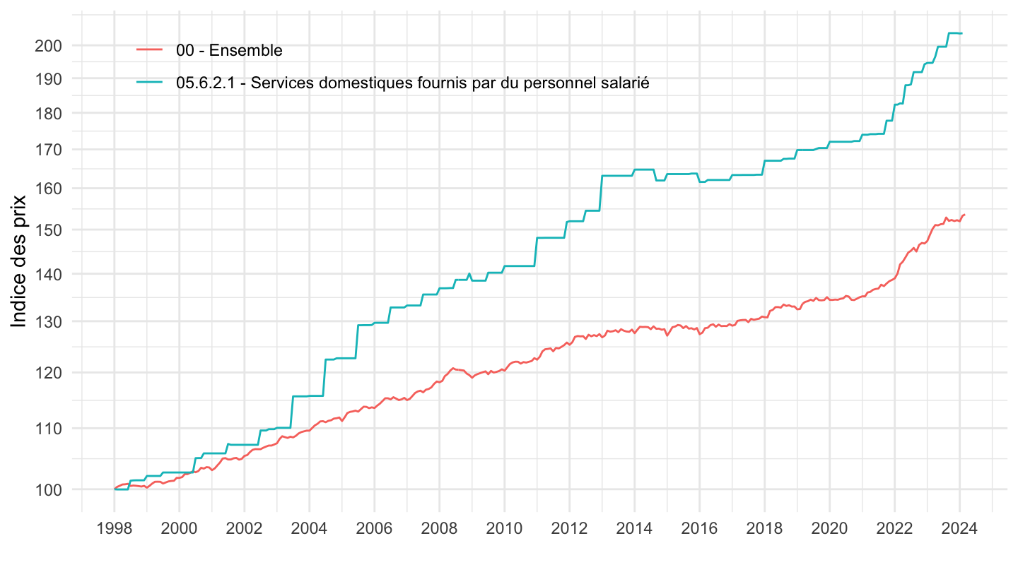
Tabac
Tabac vs. Ensemble
1990-
Code
`IPC-2015` %>%
  filter(INDICATEUR == "IPC",
         MENAGES_IPC == "ENSEMBLE",
         PRIX_CONSO %in% c("SO"),
         COICOP2016 %in% c("022", "00"),
         FREQ == "M",
         REF_AREA == "FE",
         NATURE == "INDICE") %>%
  month_to_date %>%
  arrange(date) %>%

  group_by(Coicop2016) %>%
  arrange(date) %>%
  mutate(OBS_VALUE = 100*OBS_VALUE/OBS_VALUE[1]) %>%
  ggplot() + ylab("Indice des prix") + xlab("") + theme_minimal() +
  geom_line(aes(x = date, y = OBS_VALUE, color = Coicop2016)) +

  scale_x_date(breaks = seq(1920, 2100, 5) %>% paste0("-01-01") %>% as.Date,
               labels = date_format("%Y")) +
  theme(legend.position = c(0.15, 0.9),
        legend.title = element_blank()) +
  scale_y_log10(breaks = c(100, 164, 200, 400, 600, 800, 1000),
                     labels = dollar_format(accuracy = 1, prefix = "")) +
  geom_text(data = . %>%
              filter(date == max(date)), aes(x = date, y = OBS_VALUE, label = round(OBS_VALUE, 1)), size = 3)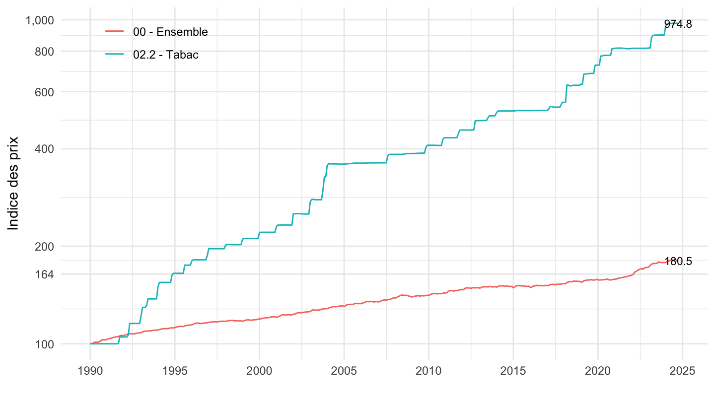
1992-2022
Code
`IPC-2015` %>%
  filter(INDICATEUR == "IPC",
         MENAGES_IPC == "ENSEMBLE",
         PRIX_CONSO == "SO",
         COICOP2016 %in% c("022", "00"),
         FREQ == "M",
         REF_AREA == "FE",
         NATURE == "INDICE") %>%
  month_to_date %>%
  arrange(date) %>%

  group_by(Coicop2016) %>%
  arrange(date) %>%
  filter(date >= as.Date("1992-01-01"),
         date <= as.Date("2022-01-01")) %>%
  mutate(OBS_VALUE = 100*OBS_VALUE/OBS_VALUE[1]) %>%
  mutate(Coicop2016 = factor(Coicop2016, levels = c("02.2 - Tabac", "00 - Ensemble"), labels = c("Tabac", "Ensemble de l'IPC"))) %>%
  ggplot() + ylab("Indice des prix (100 = Janvier 1992)") + xlab("") + theme_minimal() +
  geom_line(aes(x = date, y = OBS_VALUE, color = Coicop2016), size = 1) +

  scale_x_date(breaks = seq(1992, 2100, 5) %>% paste0("-01-01") %>% as.Date,
               labels = date_format("%Y")) +
  scale_color_manual(values = viridis(3)[1:2]) +
  theme(legend.position = c(0.15, 0.9),
        legend.title = element_blank()) +
  scale_y_log10(breaks = c(100, 200, 400, 600, 800, 1000),
                     labels = dollar_format(accuracy = 1, prefix = "")) +
  geom_label(data = . %>%
              filter(date == max(date)), aes(x = date, y = OBS_VALUE, label = round(OBS_VALUE, 1), color = Coicop2016), size = 4, show.legend = F)
1992-
Code
`IPC-2015` %>%
  filter(INDICATEUR == "IPC",
         MENAGES_IPC == "ENSEMBLE",
         COICOP2016 %in% c("022", "00"),
         FREQ == "M",
         PRIX_CONSO == "SO",
         REF_AREA == "FE",
         NATURE == "INDICE") %>%
  month_to_date %>%
  filter(date >= as.Date("1992-01-01")) %>%

  group_by(Coicop2016) %>%
  arrange(date) %>%
  mutate(OBS_VALUE = 100*OBS_VALUE/OBS_VALUE[1]) %>%
  ggplot() + ylab("Indice des prix") + xlab("") + theme_minimal() +
  geom_line(aes(x = date, y = OBS_VALUE, color = Coicop2016)) +

  scale_x_date(breaks = seq(1920, 2100, 2) %>% paste0("-01-01") %>% as.Date,
               labels = date_format("%Y")) +
  theme(legend.position = c(0.25, 0.8),
        legend.title = element_blank()) +
  scale_y_log10(breaks = c(100, 164, 200, 400, 816),
                     labels = dollar_format(accuracy = 1, prefix = "")) +
  geom_text(data = . %>%
              filter(date == max(date)), aes(x = date, y = OBS_VALUE, label = round(OBS_VALUE, 1), color = Coicop2016), size = 3, show.legend = F)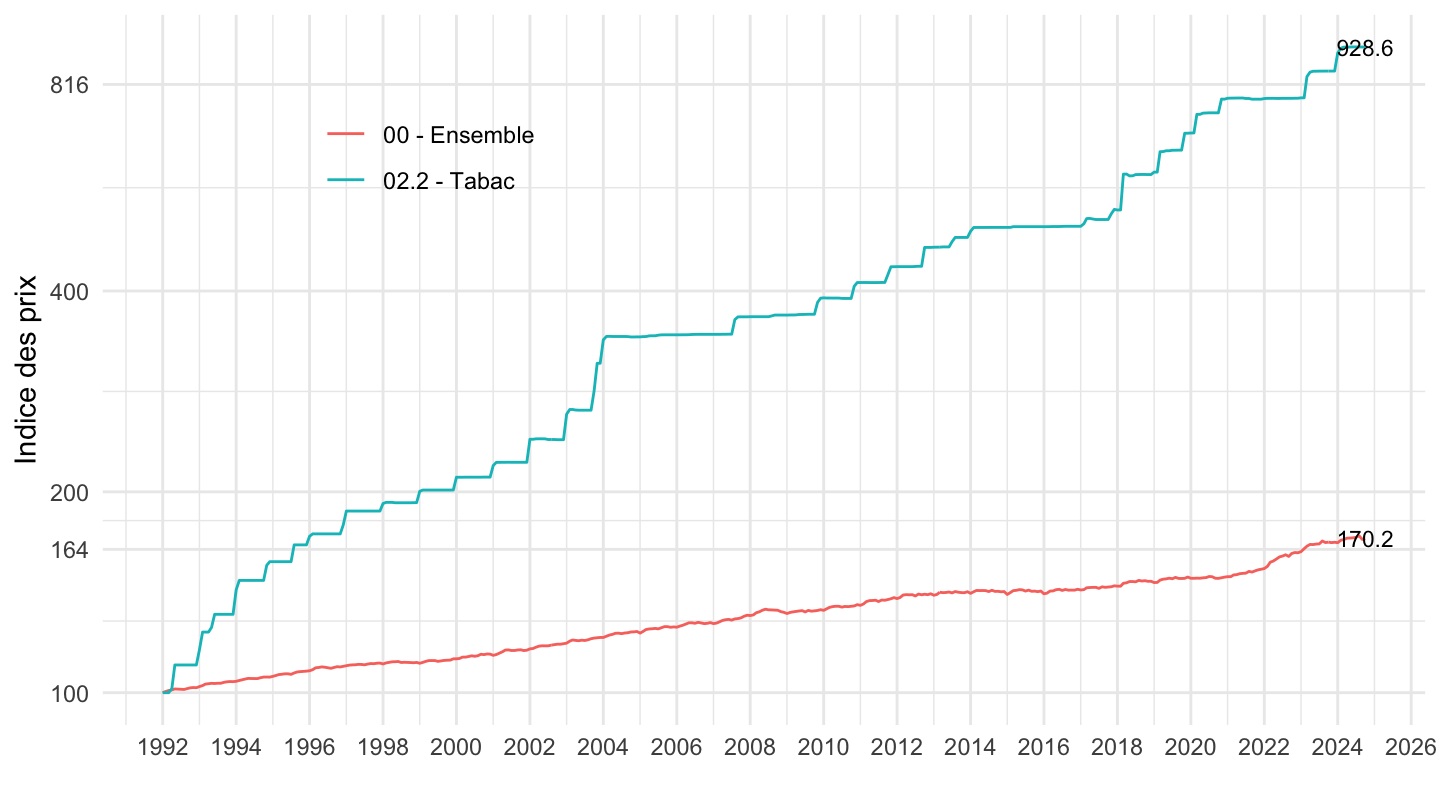
1996-
Code
`IPC-2015` %>%
  filter(INDICATEUR == "IPC",
         MENAGES_IPC == "ENSEMBLE",
         COICOP2016 %in% c("022", "00"),
         FREQ == "M",
         PRIX_CONSO == "SO",
         REF_AREA == "FE",
         NATURE == "INDICE") %>%
  month_to_date %>%
  filter(date >= as.Date("1996-01-01")) %>%

  group_by(Coicop2016) %>%
  arrange(date) %>%
  mutate(OBS_VALUE = 100*OBS_VALUE/OBS_VALUE[1]) %>%
  ggplot() + ylab("Indice des prix") + xlab("") + theme_minimal() +
  geom_line(aes(x = date, y = OBS_VALUE, color = Coicop2016)) +

  scale_x_date(breaks = seq(1920, 2100, 2) %>% paste0("-01-01") %>% as.Date,
               labels = date_format("%Y")) +
  theme(legend.position = c(0.25, 0.8),
        legend.title = element_blank()) +
  scale_y_log10(breaks = seq(100, 1000, 100),
                     labels = dollar_format(accuracy = 1, prefix = "")) +
  geom_text(data = . %>%
              filter(date == max(date)), aes(x = date, y = OBS_VALUE, label = round(OBS_VALUE, 1), color = Coicop2016), size = 3, show.legend = F)
2000-
Code
`IPC-2015` %>%
  filter(INDICATEUR == "IPC",
         MENAGES_IPC == "ENSEMBLE",
         COICOP2016 %in% c("022", "00"),
         FREQ == "M",
         PRIX_CONSO == "SO",
         REF_AREA == "FE",
         NATURE == "INDICE") %>%
  month_to_date %>%
  filter(date >= as.Date("2000-01-01")) %>%

  group_by(Coicop2016) %>%
  arrange(date) %>%
  mutate(OBS_VALUE = 100*OBS_VALUE/OBS_VALUE[1]) %>%
  ggplot() + ylab("Indice des prix") + xlab("") + theme_minimal() +
  geom_line(aes(x = date, y = OBS_VALUE, color = Coicop2016)) +

  scale_x_date(breaks = seq(1920, 2100, 2) %>% paste0("-01-01") %>% as.Date,
               labels = date_format("%Y")) +
  theme(legend.position = c(0.25, 0.8),
        legend.title = element_blank()) +
  scale_y_log10(breaks = c(seq(0, 100, 20), seq(0, 1000, 50)),
                     labels = dollar_format(accuracy = 1, prefix = "")) +
  geom_text(data = . %>%
              filter(date == max(date)), aes(x = date, y = OBS_VALUE, label = round(OBS_VALUE, 1), color = Coicop2016), size = 3, show.legend = F)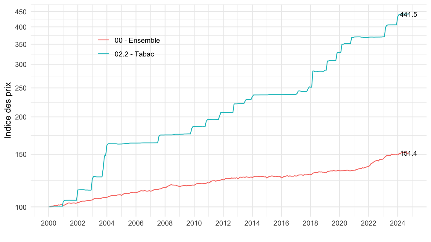
2012-
Code
`IPC-2015` %>%
  filter(INDICATEUR == "IPC",
         MENAGES_IPC == "ENSEMBLE",
         COICOP2016 %in% c("022", "00"),
         FREQ == "M",
         PRIX_CONSO == "SO",
         REF_AREA == "FE",
         NATURE == "INDICE") %>%
  month_to_date %>%
  filter(date >= as.Date("2012-01-01")) %>%

  group_by(Coicop2016) %>%
  arrange(date) %>%
  mutate(OBS_VALUE = 100*OBS_VALUE/OBS_VALUE[1]) %>%
  ggplot() + ylab("Indice des prix") + xlab("") + theme_minimal() +
  geom_line(aes(x = date, y = OBS_VALUE, color = Coicop2016)) +

  scale_x_date(breaks = seq(1920, 2100, 1) %>% paste0("-01-01") %>% as.Date,
               labels = date_format("%Y")) +
  theme(legend.position = c(0.25, 0.8),
        legend.title = element_blank()) +
  scale_y_log10(breaks = c(seq(0, 100, 10), seq(0, 1000, 10)),
                     labels = dollar_format(accuracy = 1, prefix = "")) +
  geom_text(data = . %>%
              filter(date == max(date)), aes(x = date, y = OBS_VALUE, label = round(OBS_VALUE, 1), color = Coicop2016), size = 3, show.legend = F)
2017-
Code
`IPC-2015` %>%
  filter(INDICATEUR == "IPC",
         MENAGES_IPC == "ENSEMBLE",
         COICOP2016 %in% c("022", "00"),
         FREQ == "M",
         PRIX_CONSO == "SO",
         REF_AREA == "FE",
         NATURE == "INDICE") %>%
  month_to_date %>%
  filter(date >= as.Date("2017-01-01")) %>%

  group_by(Coicop2016) %>%
  arrange(date) %>%
  mutate(OBS_VALUE = 100*OBS_VALUE/OBS_VALUE[1]) %>%
  ggplot() + ylab("Indice des prix") + xlab("") + theme_minimal() +
  geom_line(aes(x = date, y = OBS_VALUE, color = Coicop2016)) +

  scale_x_date(breaks = seq(1920, 2100, 1) %>% paste0("-01-01") %>% as.Date,
               labels = date_format("%Y")) +
  theme(legend.position = c(0.25, 0.8),
        legend.title = element_blank()) +
  scale_y_log10(breaks = c(seq(0, 100, 10), seq(0, 1000, 10)),
                     labels = dollar_format(accuracy = 1, prefix = "")) +
  geom_label(data = . %>%
              filter(date == max(date)), aes(x = date, y = OBS_VALUE, label = round(OBS_VALUE, 1), color = Coicop2016), size = 3, show.legend = F)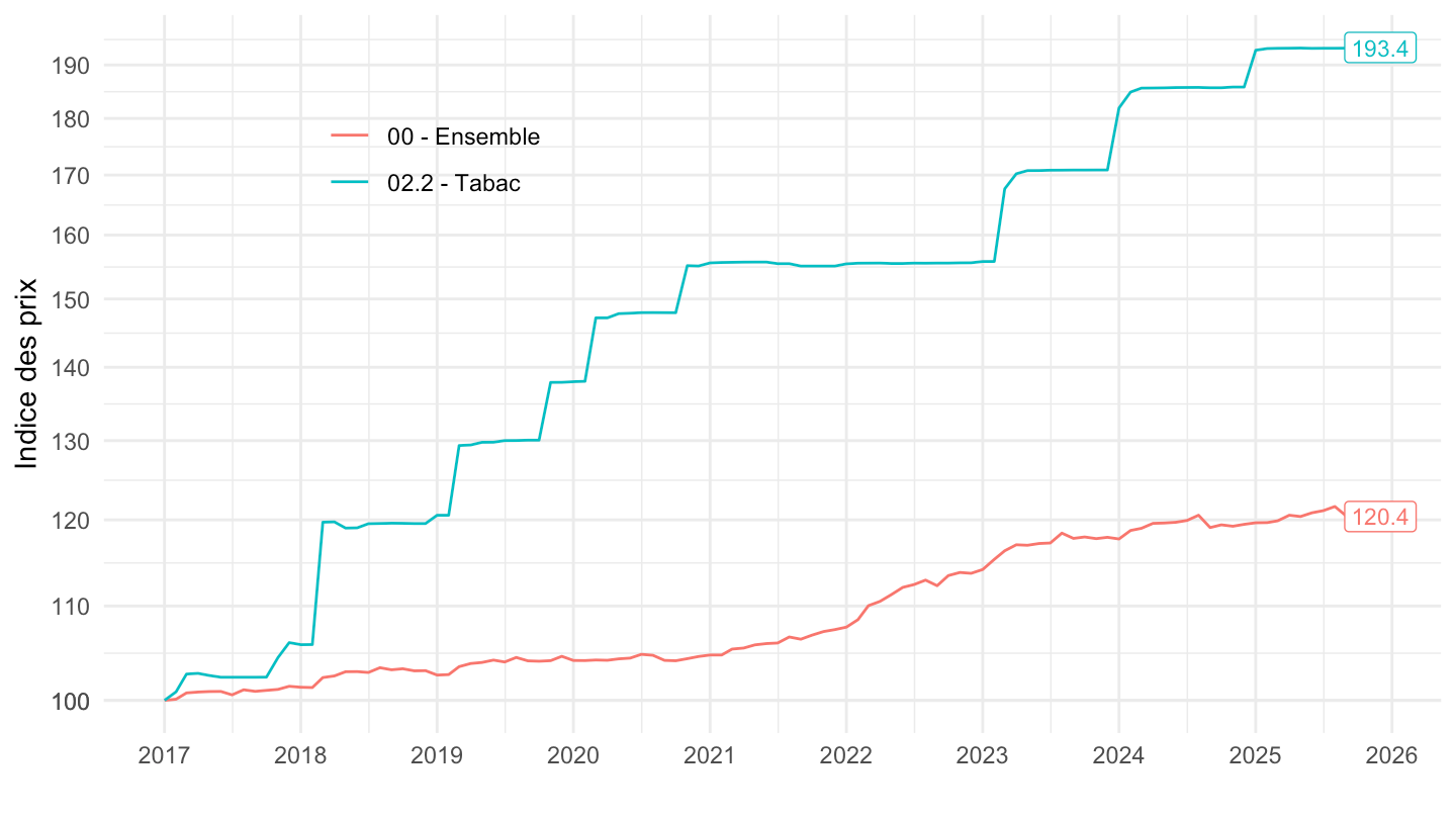
Tabac, Alcool
2017-
Code
`IPC-2015` %>%
  filter(INDICATEUR == "IPC",
         MENAGES_IPC == "ENSEMBLE",
         COICOP2016 %in% c("022", "00", "021"),
         FREQ == "M",
         PRIX_CONSO == "SO",
         REF_AREA == "FE",
         NATURE == "INDICE") %>%
  month_to_date %>%
  filter(date >= as.Date("2017-01-01")) %>%

  group_by(Coicop2016) %>%
  arrange(date) %>%
  mutate(OBS_VALUE = 100*OBS_VALUE/OBS_VALUE[1]) %>%
  ggplot() + ylab("Indice des prix") + xlab("") + theme_minimal() +
  geom_line(aes(x = date, y = OBS_VALUE, color = Coicop2016)) +

  scale_x_date(breaks = seq(1920, 2100, 1) %>% paste0("-01-01") %>% as.Date,
               labels = date_format("%Y")) +
  theme(legend.position = c(0.25, 0.8),
        legend.title = element_blank()) +
  scale_y_log10(breaks = c(seq(0, 100, 10), seq(0, 1000, 10)),
                     labels = dollar_format(accuracy = 1, prefix = "")) +
  geom_label_repel(data = . %>%
              filter(date == max(date)), aes(x = date, y = OBS_VALUE, label = round(OBS_VALUE, 1), color = Coicop2016), size = 3, show.legend = F)
Ensemble avec Tabac (IdBank: 001763852, 001759970)
1990-
Code
`IPC-2015` %>%
  filter(IDBANK %in% c("001759970", "001763852")) %>%
  month_to_date %>%
  arrange(date) %>%
  filter(date >= as.Date("1990-01-01")) %>%

  group_by(Prix_conso) %>%
  arrange(date) %>%
  mutate(OBS_VALUE = 100*OBS_VALUE/OBS_VALUE[1]) %>%
  ggplot() + ylab("Indice des prix") + xlab("") + theme_minimal() +
  geom_line(aes(x = date, y = OBS_VALUE, color = Prix_conso)) +

  scale_x_date(breaks = seq(1920, 2100, 5) %>% paste0("-01-01") %>% as.Date,
               labels = date_format("%Y")) +
  theme(legend.position = c(0.75, 0.3),
        legend.title = element_blank()) +
  scale_y_log10(breaks = seq(0, 200, 10),
                     labels = dollar_format(accuracy = 1, prefix = "")) +
  geom_text(data = . %>%
              filter(date == max(date)), aes(x = date, y = OBS_VALUE, label = round(OBS_VALUE, 1)), size = 3)
1992-
Code
`IPC-2015` %>%
  filter(INDICATEUR == "IPC",
         MENAGES_IPC == "ENSEMBLE",
         PRIX_CONSO %in% c("4035", "4018", "00"),
         FREQ == "M",
         REF_AREA == "FE",
         NATURE == "INDICE") %>%
  month_to_date %>%
  filter(date >= as.Date("1992-01-01")) %>%

  group_by(Prix_conso) %>%
  arrange(date) %>%
  mutate(OBS_VALUE = 100*OBS_VALUE/OBS_VALUE[1]) %>%
  ggplot() + ylab("Indice des prix") + xlab("") + theme_minimal() +
  geom_line(aes(x = date, y = OBS_VALUE, color = Prix_conso)) +

  scale_x_date(breaks = seq(1920, 2100, 2) %>% paste0("-01-01") %>% as.Date,
               labels = date_format("%Y")) +
  theme(legend.position = c(0.75, 0.3),
        legend.title = element_blank()) +
  scale_y_log10(breaks = seq(0, 200, 10),
                     labels = dollar_format(accuracy = 1, prefix = "")) +
  geom_text_repel(data = . %>%
              filter(date == max(date)), aes(x = date, y = OBS_VALUE, label = round(OBS_VALUE, 1)), size = 3)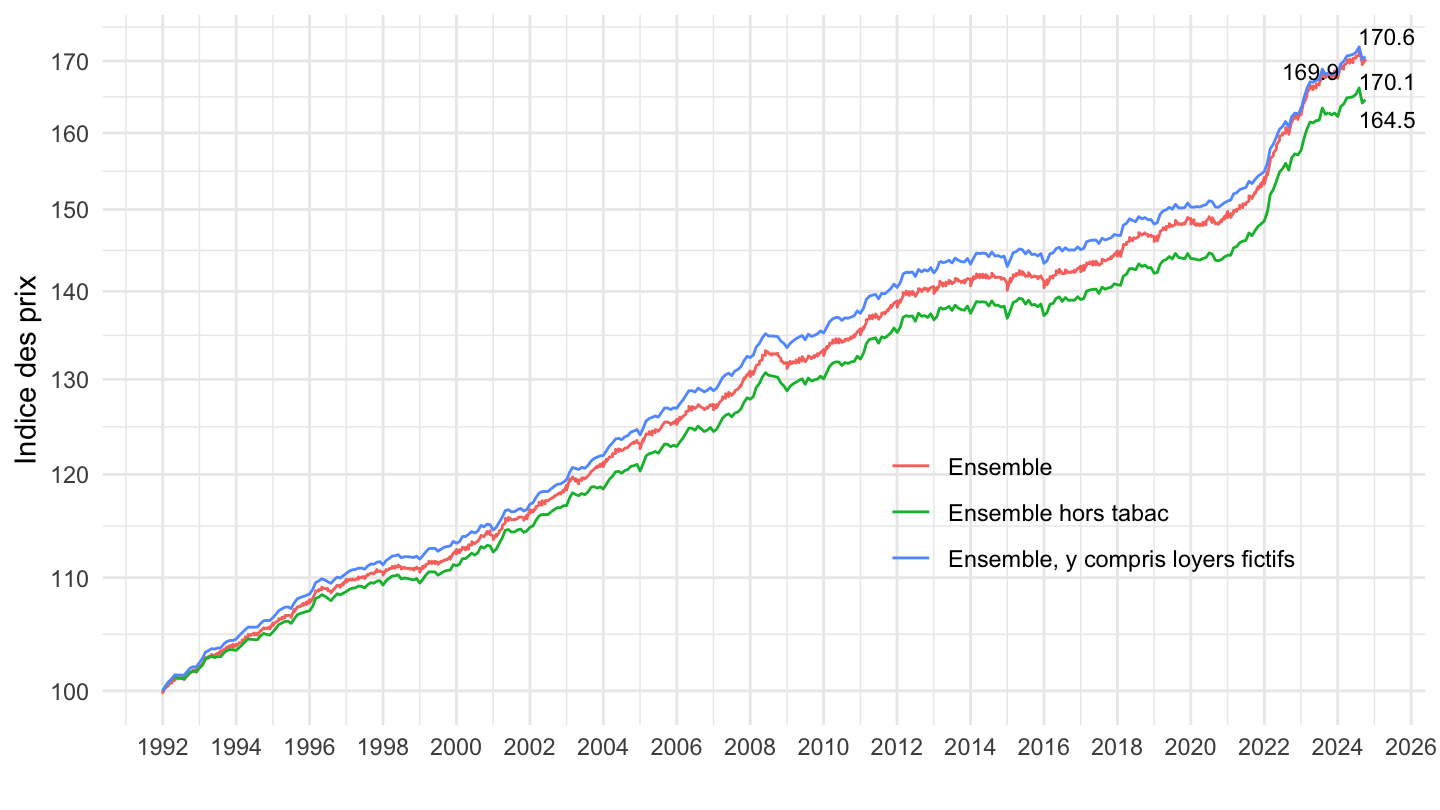
1996-
Code
`IPC-2015` %>%
  filter(INDICATEUR == "IPC",
         MENAGES_IPC == "ENSEMBLE",
         PRIX_CONSO %in% c("4035", "4018", "00"),
         FREQ == "M",
         REF_AREA == "FE",
         NATURE == "INDICE") %>%
  month_to_date %>%
  filter(date >= as.Date("1996-01-01")) %>%

  group_by(Prix_conso) %>%
  arrange(date) %>%
  mutate(OBS_VALUE = 100*OBS_VALUE/OBS_VALUE[1]) %>%
  ggplot() + ylab("Indice des prix") + xlab("") + theme_minimal() +
  geom_line(aes(x = date, y = OBS_VALUE, color = Prix_conso)) +

  scale_x_date(breaks = seq(1920, 2100, 2) %>% paste0("-01-01") %>% as.Date,
               labels = date_format("%Y")) +
  theme(legend.position = c(0.75, 0.3),
        legend.title = element_blank()) +
  scale_y_log10(breaks = seq(0, 200, 10),
                     labels = dollar_format(accuracy = 1, prefix = "")) +
  geom_text_repel(data = . %>%
              filter(date == max(date)), aes(x = date, y = OBS_VALUE, label = round(OBS_VALUE, 1)), size = 3)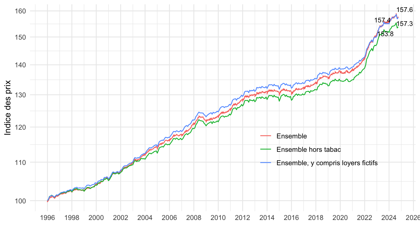
2000-
Code
`IPC-2015` %>%
  filter(INDICATEUR == "IPC",
         MENAGES_IPC == "ENSEMBLE",
         PRIX_CONSO %in% c("4035", "4018", "00"),
         FREQ == "M",
         REF_AREA == "FE",
         NATURE == "INDICE") %>%
  month_to_date %>%
  filter(date >= as.Date("2000-01-01")) %>%

  group_by(Prix_conso) %>%
  arrange(date) %>%
  mutate(OBS_VALUE = 100*OBS_VALUE/OBS_VALUE[1]) %>%
  ggplot() + ylab("Indice des prix") + xlab("") + theme_minimal() +
  geom_line(aes(x = date, y = OBS_VALUE, color = Prix_conso)) +

  scale_x_date(breaks = seq(1920, 2100, 2) %>% paste0("-01-01") %>% as.Date,
               labels = date_format("%Y")) +
  theme(legend.position = c(0.75, 0.3),
        legend.title = element_blank()) +
  scale_y_log10(breaks = seq(0, 200, 5),
                     labels = dollar_format(accuracy = 1, prefix = "")) +
  geom_text_repel(data = . %>%
              filter(date == max(date)), aes(x = date, y = OBS_VALUE, label = round(OBS_VALUE, 1)), size = 3)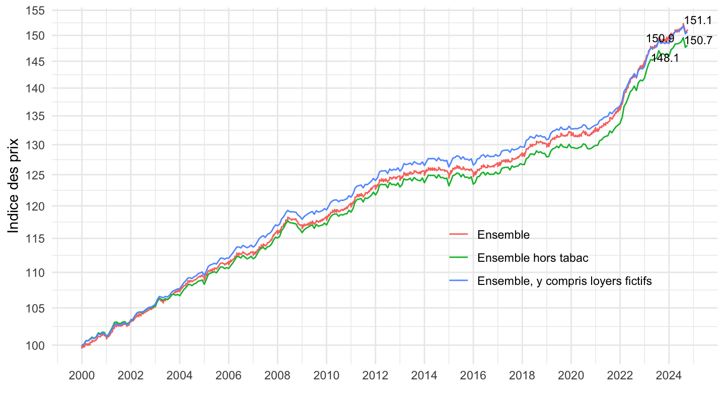
2012-
Code
`IPC-2015` %>%
  filter(INDICATEUR == "IPC",
         MENAGES_IPC == "ENSEMBLE",
         PRIX_CONSO %in% c("4035", "4018", "00"),
         FREQ == "M",
         REF_AREA == "FE",
         NATURE == "INDICE") %>%
  month_to_date %>%
  filter(date >= as.Date("2012-01-01")) %>%

  group_by(Prix_conso) %>%
  arrange(date) %>%
  mutate(OBS_VALUE = 100*OBS_VALUE/OBS_VALUE[1]) %>%
  ggplot() + ylab("Indice des prix") + xlab("") + theme_minimal() +
  geom_line(aes(x = date, y = OBS_VALUE, color = Prix_conso)) +

  scale_x_date(breaks = seq(1920, 2100, 2) %>% paste0("-01-01") %>% as.Date,
               labels = date_format("%Y")) +
  theme(legend.position = c(0.35, 0.8),
        legend.title = element_blank()) +
  scale_y_log10(breaks = seq(0, 200, 1),
                     labels = dollar_format(accuracy = 1, prefix = "")) +
  geom_text_repel(data = . %>%
              filter(date == max(date)), aes(x = date, y = OBS_VALUE, label = round(OBS_VALUE, 1)), size = 3)
2017-
Code
`IPC-2015` %>%
  filter(INDICATEUR == "IPC",
         MENAGES_IPC == "ENSEMBLE",
         PRIX_CONSO %in% c("4035", "4018", "00"),
         FREQ == "M",
         REF_AREA == "FE",
         NATURE == "INDICE") %>%
  month_to_date %>%
  filter(date >= as.Date("2017-01-01")) %>%

  group_by(Prix_conso) %>%
  arrange(date) %>%
  mutate(OBS_VALUE = 100*OBS_VALUE/OBS_VALUE[1]) %>%
  ggplot() + ylab("Indice des prix") + xlab("") + theme_minimal() +
  geom_line(aes(x = date, y = OBS_VALUE, color = Prix_conso)) +

  scale_x_date(breaks = seq(1920, 2100, 1) %>% paste0("-01-01") %>% as.Date,
               labels = date_format("%Y")) +
  theme(legend.position = c(0.35, 0.8),
        legend.title = element_blank()) +
  scale_y_log10(breaks = seq(0, 200, 1),
                     labels = dollar_format(accuracy = 1, prefix = "")) +
  geom_text_repel(data = . %>%
              filter(date == max(date)), aes(x = date, y = OBS_VALUE, label = round(OBS_VALUE, 1)), size = 3)
Glissement sur 3 ans
Code
`IPC-2015` %>%
  filter(INDICATEUR == "IPC",
         MENAGES_IPC == "ENSEMBLE",
         PRIX_CONSO %in% c("4035", "4018"),
         FREQ == "M",
         REF_AREA == "FE",
         NATURE == "INDICE") %>%

  month_to_date %>%
  filter(date >= max(date) - years(3)) %>%
  group_by(Prix_conso) %>%
  arrange(date) %>%
  mutate(OBS_VALUE = 100*OBS_VALUE/OBS_VALUE[1]) %>%
  ggplot + geom_line(aes(x = date, y = OBS_VALUE, color = Prix_conso)) +
  theme_minimal() + xlab("") + ylab("") +
  scale_x_date(breaks = "1 month",
               labels = date_format("%b %Y")) +
  theme(legend.position = c(0.65, 0.2),
        legend.title = element_blank(),
        axis.text.x = element_text(angle = 45, vjust = 0.5, hjust=1)) +
  scale_y_log10(breaks = seq(0, 200, 1),
                     labels = dollar_format(accuracy = 1, prefix = "")) +
  geom_text_repel(aes(x = date, y = OBS_VALUE, label = round(OBS_VALUE, 1)),
                  fontface ="plain", color = "black", size = 3)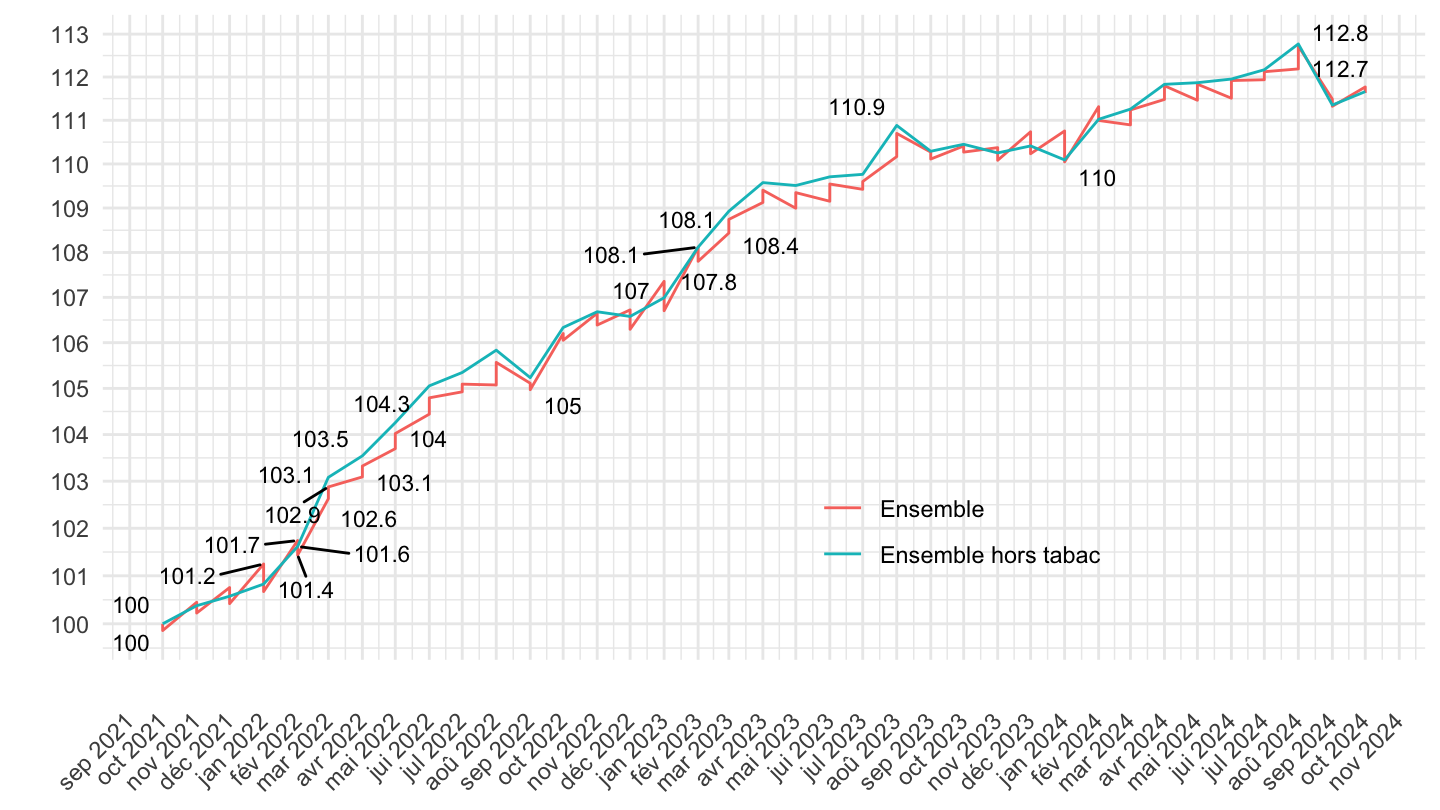
Glissement sur 2 ans
Code
`IPC-2015` %>%
  filter(INDICATEUR == "IPC",
         MENAGES_IPC == "ENSEMBLE",
         PRIX_CONSO %in% c("4035", "4018", "00"),
         FREQ == "M",
         REF_AREA == "FE",
         NATURE == "INDICE") %>%

  month_to_date %>%
  filter(date >= max(date) - years(2)) %>%
  group_by(Prix_conso) %>%
  arrange(date) %>%
  mutate(OBS_VALUE = 100*OBS_VALUE/OBS_VALUE[1]) %>%
  ggplot + geom_line(aes(x = date, y = OBS_VALUE, color = Prix_conso)) +
  theme_minimal() + xlab("") + ylab("") +
  scale_x_date(breaks = "1 month",
               labels = date_format("%b %Y")) +
  theme(legend.position = c(0.65, 0.2),
        legend.title = element_blank(),
        axis.text.x = element_text(angle = 45, vjust = 0.5, hjust=1)) +
  scale_y_log10(breaks = seq(0, 200, 1),
                     labels = dollar_format(accuracy = 1, prefix = "")) +
  geom_text_repel(aes(x = date, y = OBS_VALUE, label = round(OBS_VALUE, 1)),
                  fontface ="plain", color = "black", size = 3)
Glissement sur 1 an
Code
`IPC-2015` %>%
  filter(INDICATEUR == "IPC",
         MENAGES_IPC == "ENSEMBLE",
         PRIX_CONSO %in% c("4035", "4018", "00"),
         FREQ == "M",
         REF_AREA == "FE",
         NATURE == "INDICE") %>%

  month_to_date %>%
  filter(date >= max(date) - years(1)) %>%
  group_by(Prix_conso) %>%
  arrange(date) %>%
  mutate(OBS_VALUE = 100*OBS_VALUE/OBS_VALUE[1]) %>%
  ggplot + geom_line(aes(x = date, y = OBS_VALUE, color = Prix_conso)) +
  theme_minimal() + xlab("") + ylab("") +
  scale_x_date(breaks = "1 month",
               labels = date_format("%b %Y")) +
  theme(legend.position = c(0.65, 0.2),
        legend.title = element_blank(),
        axis.text.x = element_text(angle = 45, vjust = 0.5, hjust=1)) +
  scale_y_log10(breaks = seq(0, 200, 1),
                     labels = dollar_format(accuracy = 1, prefix = "")) +
  geom_text_repel(aes(x = date, y = OBS_VALUE, label = round(OBS_VALUE, 1)),
                  fontface ="plain", color = "black", size = 3)
Immobilier
4003, 4009, 4034
Code
`IPC-2015` %>%
  filter(INDICATEUR == "IPC",
         MENAGES_IPC == "ENSEMBLE",
         PRIX_CONSO %in% c("4003", "4009", "4034"),
         FREQ == "M",
         REF_AREA == "FE",
         NATURE == "INDICE") %>%
  month_to_date %>%

  ggplot() + ylab("Indice des prix") + xlab("") + theme_minimal() +
  geom_line(aes(x = date, y = OBS_VALUE, color = Prix_conso, linetype = Prix_conso)) +

  scale_x_date(breaks = seq(1920, 2100, 5) %>% paste0("-01-01") %>% as.Date,
               labels = date_format("%Y")) +
  theme(legend.position = c(0.75, 0.3),
        legend.title = element_blank()) +
  scale_y_log10(breaks = seq(0, 200, 10),
                     labels = dollar_format(accuracy = 1, prefix = ""))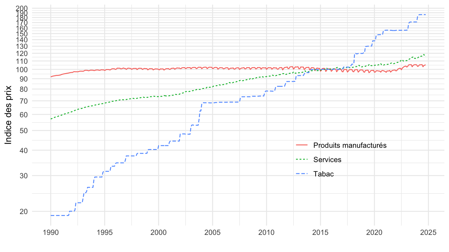
041, 043, 044
Code
`IPC-2015` %>%
  filter(INDICATEUR == "IPC",
         MENAGES_IPC == "ENSEMBLE",
         COICOP2016 %in% c("041", "043", "044"),
         FREQ == "M",
         REF_AREA == "FE",
         NATURE == "INDICE",
         #OBS_STATUS == "A"
         ) %>%
  month_to_date %>%


  ggplot() + ylab("Indice des prix") + xlab("") + theme_minimal() +
  geom_line(aes(x = date, y = OBS_VALUE, color = Coicop2016)) +

  scale_x_date(breaks = seq(1920, 2100, 5) %>% paste0("-01-01") %>% as.Date,
               labels = date_format("%Y")) +
  theme(legend.position = c(0.6, 0.3),
        legend.title = element_blank()) +
  scale_y_log10(breaks = seq(0, 200, 10),
                     labels = dollar_format(accuracy = 1, prefix = ""))
041 Loyers effectifs, 00 Ensemble
1990-
All
Code
`IPC-2015` %>%
  filter(INDICATEUR == "IPC",
         MENAGES_IPC == "ENSEMBLE",
         COICOP2016 %in% c("041", "00"),
         FREQ == "M",
         REF_AREA == "FE",
         NATURE == "INDICE") %>%
  month_to_date %>%


  group_by(Coicop2016, Prix_conso) %>%
  filter(date >= as.Date("1990-01-01")) %>%
  mutate(OBS_VALUE = 100*OBS_VALUE/OBS_VALUE[date == as.Date("1990-01-01")]) %>%
  mutate(Variable = paste0(Coicop2016, " - ", Prix_conso),
         Variable = gsub(" - Sans objet", "", Variable)) %>%
  ggplot() + ylab("Indice des prix") + xlab("") + theme_minimal() +
  geom_line(aes(x = date, y = OBS_VALUE, color = Variable)) +

  scale_x_date(breaks = seq(1920, 2100, 5) %>% paste0("-01-01") %>% as.Date,
               labels = date_format("%Y")) +
  theme(legend.position = c(0.7, 0.2),
        legend.title = element_blank()) +
  scale_y_log10(breaks = seq(0, 200, 5),
                     labels = dollar_format(accuracy = 1, prefix = ""))
Loyers, Loyers Réels, IPC
Code
`IPC-2015-2020` %>%
  filter(INDICATEUR == "IPC",
         MENAGES_IPC == "ENSEMBLE",
         COICOP2016 %in% c("041", "00"),
         FREQ == "M",
         REF_AREA == "FE",
         NATURE == "INDICE",
         #OBS_STATUS == "A"
         ) %>%
  #select(-OBS_VALUE, - TIME_PERIOD) %>%
  #distinct
  month_to_date %>%
  select(date, COICOP2016, OBS_VALUE) %>%
  spread(COICOP2016, OBS_VALUE) %>%
  mutate(`real_rents` = `041`/`00`) %>%
  gather(COICOP2016, OBS_VALUE, -date) %>%
  left_join(tibble(COICOP2016 = c("041", "00", "real_rents"),
                   Coicop2016 = c("Loyers", "IPC", "Loyers Réels")),
            by = "COICOP2016") %>%
  group_by(COICOP2016) %>%
  mutate(OBS_VALUE = 100*OBS_VALUE/OBS_VALUE[date == as.Date("1990-01-01")]) %>%
  ggplot() + ylab("Indice des prix") + xlab("") + theme_minimal() +
  geom_line(aes(x = date, y = OBS_VALUE, color = Coicop2016)) +

  scale_x_date(breaks = seq(1920, 2100, 5) %>% paste0("-01-01") %>% as.Date,
               labels = date_format("%Y")) +
  theme(legend.position = c(0.25, 0.8),
        legend.title = element_blank()) +
  scale_y_log10(breaks = seq(0, 200, 10),
                     labels = dollar_format(accuracy = 1, prefix = ""))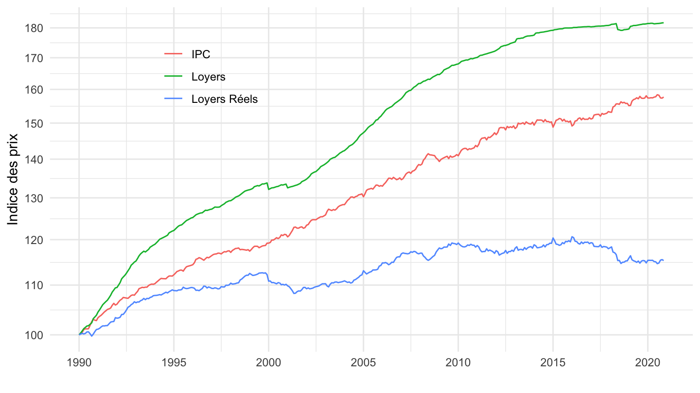
1992-
Code
`IPC-2015` %>%
  filter(INDICATEUR == "IPC",
         MENAGES_IPC == "ENSEMBLE",
         COICOP2016 %in% c("041", "00"),
         FREQ == "M",
         REF_AREA == "FE",
         NATURE == "INDICE") %>%
  month_to_date %>%


  group_by(Coicop2016, Prix_conso) %>%
  filter(date >= as.Date("1992-01-01")) %>%
  mutate(OBS_VALUE = 100*OBS_VALUE/OBS_VALUE[date == as.Date("1992-01-01")]) %>%
  mutate(Variable = paste0(Coicop2016, " - ", Prix_conso),
         Variable = gsub(" - Sans objet", "", Variable)) %>%
  ggplot() + ylab("Indice des prix") + xlab("") + theme_minimal() +
  geom_line(aes(x = date, y = OBS_VALUE, color = Variable)) +

  scale_x_date(breaks = seq(1920, 2100, 2) %>% paste0("-01-01") %>% as.Date,
               labels = date_format("%Y")) +
  theme(legend.position = c(0.7, 0.2),
        legend.title = element_blank()) +
  scale_y_log10(breaks = seq(0, 200, 5),
                     labels = dollar_format(accuracy = 1, prefix = ""))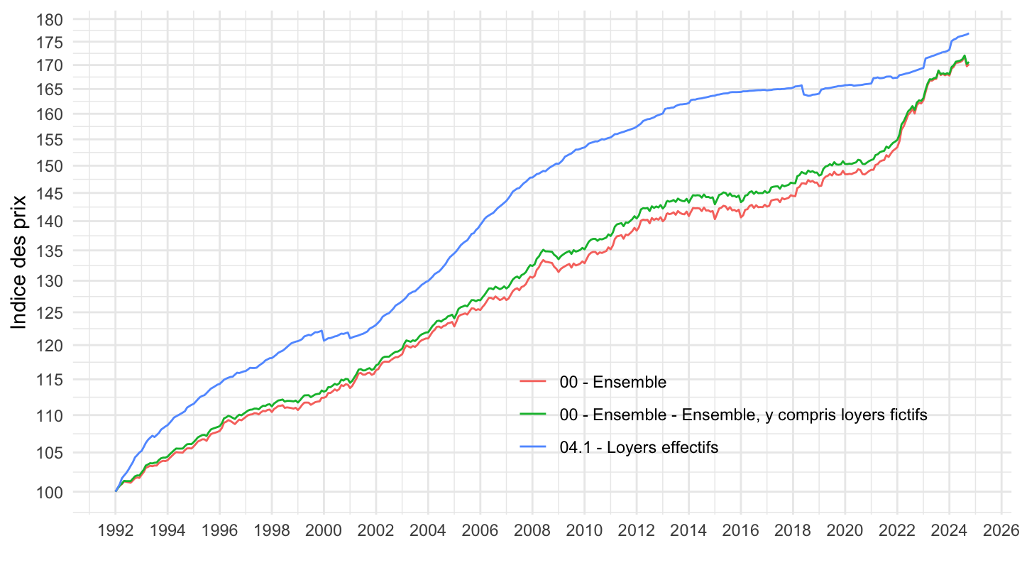
1992- (fictifs)
- Blog Loyers. Lien
Code
`IPC-2015-2020` %>%
  filter(INDICATEUR == "IPC",
         MENAGES_IPC == "ENSEMBLE",
         COICOP2016 %in% c("041", "00", "4035"),
         FREQ == "M",
         REF_AREA == "FE",
         NATURE == "INDICE",
         #OBS_STATUS == "A"
         ) %>%
  #select(-OBS_VALUE, - TIME_PERIOD) %>%
  #distinct
  month_to_date %>%


  group_by(Coicop2016) %>%
  filter(date >= as.Date("1990-01-01")) %>%
  mutate(OBS_VALUE = 100*OBS_VALUE/OBS_VALUE[date == as.Date("1992-01-01")]) %>%
  ggplot() + ylab("Indice des prix") + xlab("") + theme_minimal() +
  geom_line(aes(x = date, y = OBS_VALUE, color = Coicop2016)) +

  scale_x_date(breaks = seq(1920, 2022, 2) %>% paste0("-01-01") %>% as.Date,
               labels = date_format("%Y")) +
  theme(legend.position = c(0.75, 0.3),
        legend.title = element_blank()) +
  scale_y_log10(breaks = seq(0, 200, 10),
                     labels = dollar_format(accuracy = 1, prefix = ""))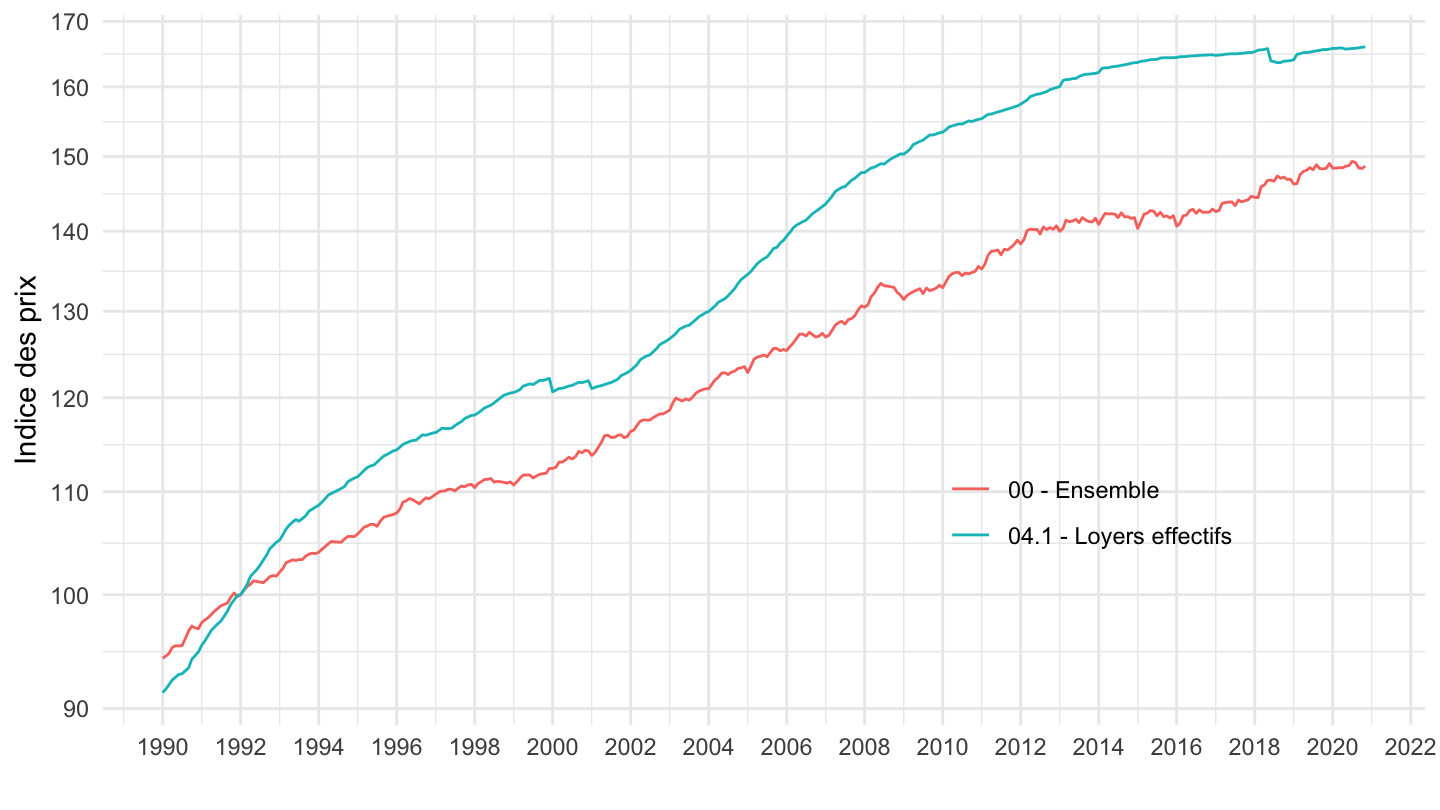
1990-
Code
`IPC-2015-2020` %>%
  filter(INDICATEUR == "IPC",
         MENAGES_IPC == "ENSEMBLE",
         COICOP2016 %in% c("041", "00", "4035"),
         FREQ == "M",
         REF_AREA == "FE",
         NATURE == "INDICE",
         #OBS_STATUS == "A"
         ) %>%
  #select(-OBS_VALUE, - TIME_PERIOD) %>%
  #distinct
  month_to_date %>%


  group_by(Coicop2016) %>%
  filter(date >= as.Date("1990-01-01")) %>%
  mutate(OBS_VALUE = 100*OBS_VALUE/OBS_VALUE[date == as.Date("1990-01-01")]) %>%
  ggplot() + ylab("Indice des prix") + xlab("") + theme_minimal() +
  geom_line(aes(x = date, y = OBS_VALUE, color = Coicop2016)) +
  scale_color_manual(values = viridis(3)[1:2]) +
  scale_x_date(breaks = seq(1920, 2022, 5) %>% paste0("-01-01") %>% as.Date,
               labels = date_format("%Y")) +
  theme(legend.position = c(0.75, 0.3),
        legend.title = element_blank()) +
  scale_y_log10(breaks = seq(0, 200, 10),
                     labels = dollar_format(accuracy = 1, prefix = ""))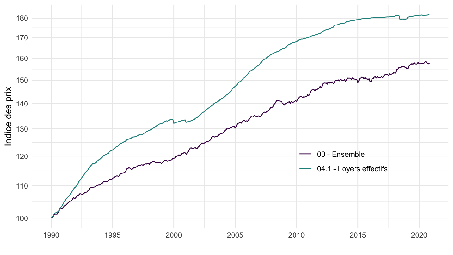
1996-
Code
`IPC-2015` %>%
  filter(INDICATEUR == "IPC",
         MENAGES_IPC == "ENSEMBLE",
         COICOP2016 %in% c("041", "00"),
         FREQ == "M",
         REF_AREA == "FE",
         NATURE == "INDICE") %>%
  month_to_date %>%


  group_by(Coicop2016, Prix_conso) %>%
  filter(date >= as.Date("1996-01-01")) %>%
  mutate(OBS_VALUE = 100*OBS_VALUE/OBS_VALUE[date == as.Date("1996-01-01")]) %>%
  mutate(Variable = paste0(Coicop2016, " - ", Prix_conso),
         Variable = gsub(" - Sans objet", "", Variable)) %>%
  ggplot() + ylab("Indice des prix") + xlab("") + theme_minimal() +
  geom_line(aes(x = date, y = OBS_VALUE, color = Variable)) +

  scale_x_date(breaks = seq(1920, 2100, 2) %>% paste0("-01-01") %>% as.Date,
               labels = date_format("%Y")) +
  theme(legend.position = c(0.7, 0.2),
        legend.title = element_blank()) +
  scale_y_log10(breaks = seq(0, 200, 5),
                     labels = dollar_format(accuracy = 1, prefix = ""))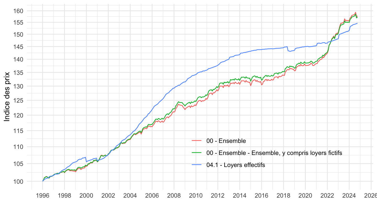
1990-1999
Code
`IPC-2015` %>%
  filter(INDICATEUR == "IPC",
         MENAGES_IPC == "ENSEMBLE",
         COICOP2016 %in% c("041", "00"),
         FREQ == "M",
         REF_AREA == "FE",
         NATURE == "INDICE") %>%
  month_to_date %>%


  group_by(Coicop2016, Prix_conso) %>%
  filter(date >= as.Date("1990-01-01"),
         date <= as.Date("1999-01-01")) %>%
  mutate(OBS_VALUE = 100*OBS_VALUE/OBS_VALUE[date == as.Date("1990-01-01")]) %>%
  mutate(Variable = paste0(Coicop2016, " - ", Prix_conso),
         Variable = gsub(" - Sans objet", "", Variable)) %>%
  ggplot() + ylab("Indice des prix") + xlab("") + theme_minimal() +
  geom_line(aes(x = date, y = OBS_VALUE, color = Variable)) +

  scale_x_date(breaks = seq(1920, 2100, 1) %>% paste0("-01-01") %>% as.Date,
               labels = date_format("%Y")) +
  theme(legend.position = c(0.35, 0.85),
        legend.title = element_blank()) +
  scale_y_log10(breaks = seq(0, 200, 5),
                     labels = dollar_format(accuracy = 1, prefix = ""))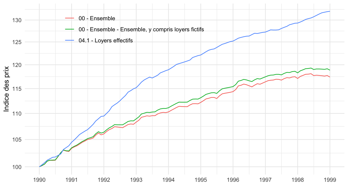
1999-
Code
`IPC-2015` %>%
  filter(INDICATEUR == "IPC",
         MENAGES_IPC == "ENSEMBLE",
         COICOP2016 %in% c("041", "00"),
         FREQ == "M",
         REF_AREA == "FE",
         NATURE == "INDICE") %>%
  month_to_date %>%


  group_by(Coicop2016, Prix_conso) %>%
  filter(date >= as.Date("1999-01-01")) %>%
  mutate(OBS_VALUE = 100*OBS_VALUE/OBS_VALUE[date == as.Date("1999-01-01")]) %>%
  ggplot() + ylab("Indice des prix") + xlab("") + theme_minimal() +
  geom_line(aes(x = date, y = OBS_VALUE, color = paste0(Coicop2016, " - ", Prix_conso))) +

  scale_x_date(breaks = seq(1920, 2100, 2) %>% paste0("-01-01") %>% as.Date,
               labels = date_format("%Y")) +
  theme(legend.position = c(0.7, 0.2),
        legend.title = element_blank()) +
  scale_y_log10(breaks = seq(0, 200, 5),
                     labels = dollar_format(accuracy = 1, prefix = ""))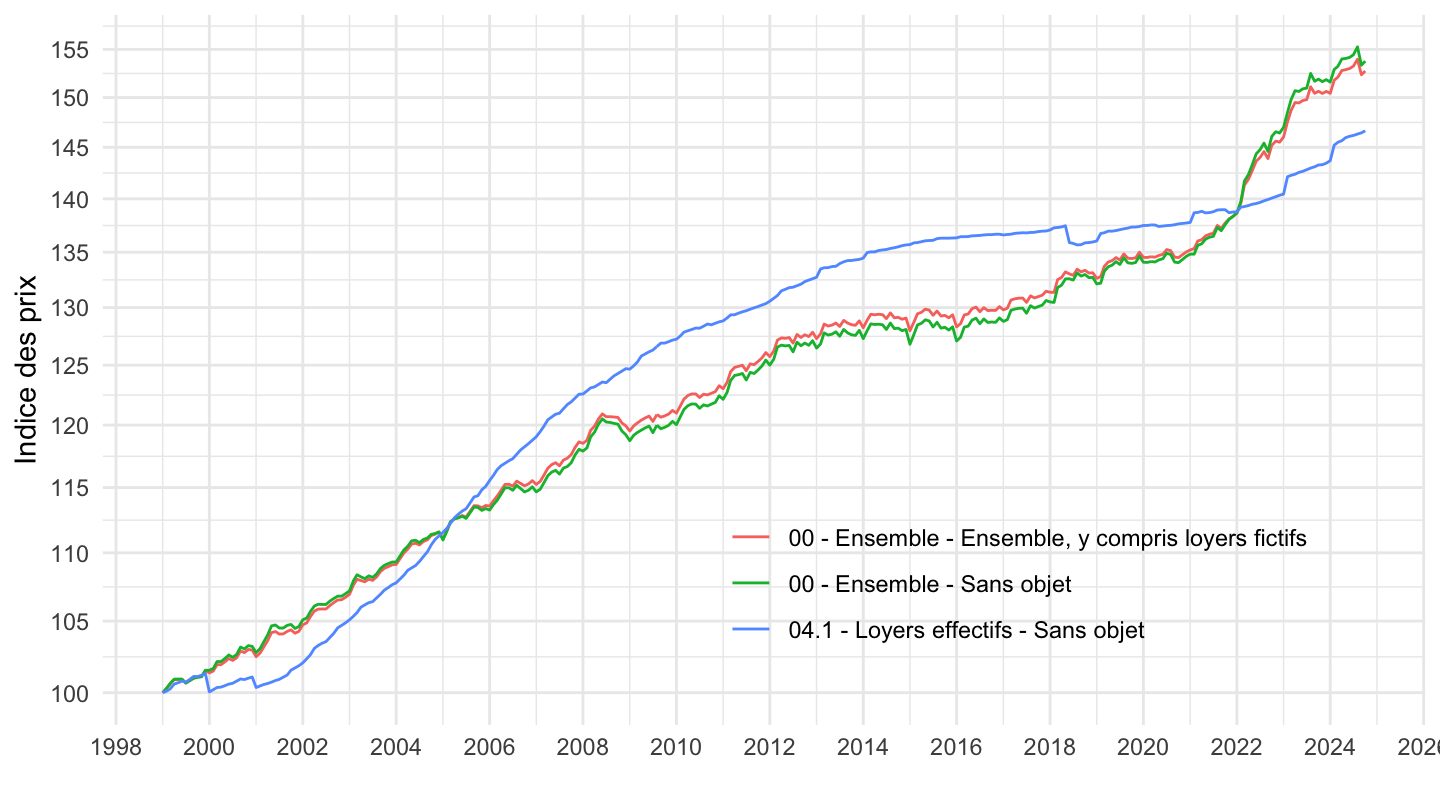
2000-
Code
`IPC-2015` %>%
  filter(INDICATEUR == "IPC",
         MENAGES_IPC == "ENSEMBLE",
         COICOP2016 %in% c("041", "00"),
         FREQ == "M",
         REF_AREA == "FE",
         NATURE == "INDICE") %>%
  month_to_date %>%


  group_by(Coicop2016, Prix_conso) %>%
  filter(date >= as.Date("2000-01-01")) %>%
  mutate(OBS_VALUE = 100*OBS_VALUE/OBS_VALUE[date == as.Date("2000-01-01")]) %>%
  ggplot() + ylab("Indice des prix") + xlab("") + theme_minimal() +
  geom_line(aes(x = date, y = OBS_VALUE, color = paste0(Coicop2016, " - ", Prix_conso))) +

  scale_x_date(breaks = seq(1920, 2100, 2) %>% paste0("-01-01") %>% as.Date,
               labels = date_format("%Y")) +
  theme(legend.position = c(0.7, 0.2),
        legend.title = element_blank()) +
  scale_y_log10(breaks = seq(0, 200, 5),
                     labels = dollar_format(accuracy = 1, prefix = ""))
2017-
Code
`IPC-2015` %>%
  filter(INDICATEUR == "IPC",
         MENAGES_IPC == "ENSEMBLE",
         COICOP2016 %in% c("041", "00"),
         FREQ == "M",
         REF_AREA == "FE",
         NATURE == "INDICE") %>%
  month_to_date %>%


  group_by(Coicop2016, Prix_conso) %>%
  filter(date >= as.Date("2017-01-01")) %>%
  mutate(OBS_VALUE = 100*OBS_VALUE/OBS_VALUE[date == as.Date("2017-01-01")]) %>%
  ggplot() + ylab("Base 100 = Janvier 2017") + xlab("") + theme_minimal() +
  geom_line(aes(x = date, y = OBS_VALUE, color = paste0(Coicop2016, " - ", Prix_conso))) +

  scale_x_date(breaks = seq(1920, 2100, 1) %>% paste0("-01-01") %>% as.Date,
               labels = date_format("%Y")) +
  theme(legend.position = c(0.35, 0.8),
        legend.title = element_blank()) +
  scale_y_log10(breaks = seq(0, 200, 2),
                     labels = dollar_format(accuracy = 1, prefix = ""))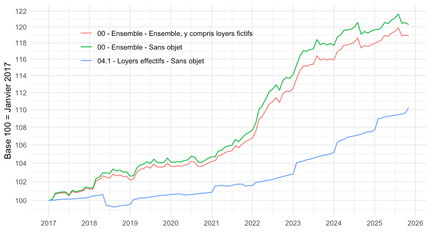
Glissement sur 2 ans
Code
`IPC-2015` %>%
  filter(INDICATEUR == "IPC",
         MENAGES_IPC == "ENSEMBLE",
         COICOP2016 %in% c("041", "00"),
         FREQ == "M",
         REF_AREA == "FE",
         NATURE == "INDICE") %>%
  month_to_date %>%
  filter(date >= max(date) - years(2)) %>%


  group_by(COICOP2016) %>%
  arrange(date) %>%
  mutate(OBS_VALUE = 100*OBS_VALUE/OBS_VALUE[1]) %>%
  ggplot() + ylab("Indice des prix") + xlab("") + theme_minimal() +
  geom_line(aes(x = date, y = OBS_VALUE, color = paste0(Coicop2016, " - ", Prix_conso))) +
  theme_minimal() + xlab("") + ylab("") +
  scale_x_date(breaks = "1 month",
               labels = date_format("%b %Y")) +
  theme(legend.position = c(0.28, 0.87),
        legend.title = element_blank(),
        axis.text.x = element_text(angle = 45, vjust = 0.5, hjust=1)) +
  scale_y_log10(breaks = seq(0, 200, 2),
                     labels = dollar_format(accuracy = 1, prefix = "")) +
  geom_text_repel(aes(x = date, y = OBS_VALUE, label = round(OBS_VALUE, 1)),
                  fontface ="plain", color = "black", size = 3)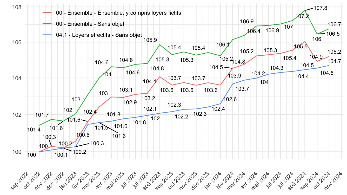
Insee calcule y compris loyers fictifs
1990-
Code
`IPC-2015` %>%
  filter(INDICATEUR == "IPC",
         REF_AREA == "FE",
         PRIX_CONSO %in% c("00", "4035"),
         #PRIX_CONSO %in% c("00"),
         NATURE == "INDICE",
         FREQ == "M") %>%
  month_to_date %>%
  group_by(PRIX_CONSO) %>%
  mutate(OBS_VALUE = 100*OBS_VALUE / OBS_VALUE[date == as.Date("1990-01-01")]) %>%

  ggplot() + ylab("Indice des prix") + xlab("") + theme_minimal() +
  geom_line(aes(x = date, y = OBS_VALUE, color = Prix_conso)) +

  scale_x_date(breaks = seq(1920, 2100, 5) %>% paste0("-01-01") %>% as.Date,
               labels = date_format("%Y")) +
  theme(legend.position = c(0.75, 0.3),
        legend.title = element_blank()) +
  scale_y_log10(breaks = seq(0, 200, 10),
                     labels = dollar_format(accuracy = 1, prefix = "")) +
  geom_text_repel(data = . %>%
              filter(date == max(date)), aes(x = date, y = OBS_VALUE, label = round(OBS_VALUE, 1)), size = 3)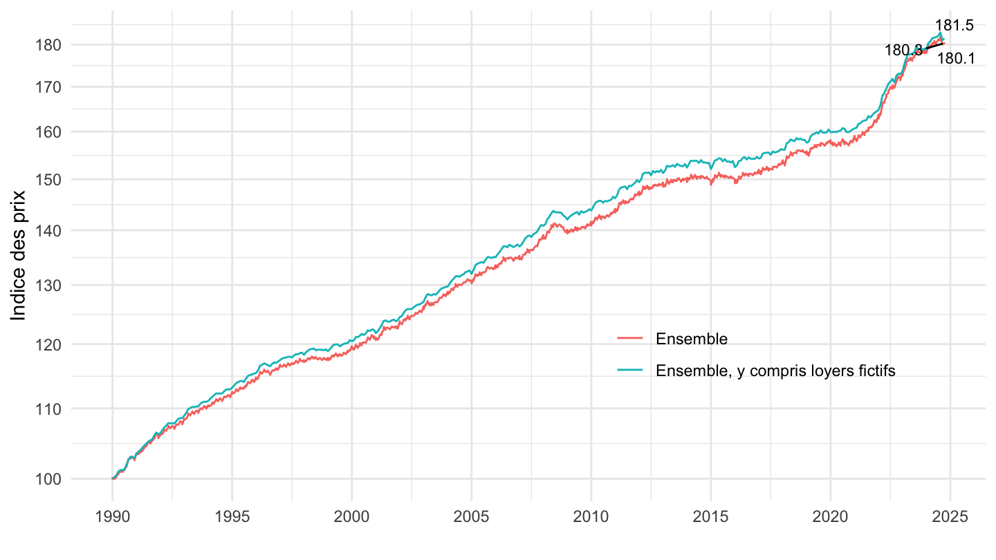
1992-
Code
`IPC-2015` %>%
  filter(INDICATEUR == "IPC",
         REF_AREA == "FE",
         PRIX_CONSO %in% c("00", "4035"),
         #PRIX_CONSO %in% c("00"),
         NATURE == "INDICE",
         FREQ == "M") %>%
  month_to_date %>%
  group_by(PRIX_CONSO) %>%
  mutate(OBS_VALUE = 100*OBS_VALUE / OBS_VALUE[date == as.Date("1992-01-01")]) %>%
  filter(date >= as.Date("1992-01-01")) %>%

  ggplot() + ylab("Indice des prix") + xlab("") + theme_minimal() +
  geom_line(aes(x = date, y = OBS_VALUE, color = Prix_conso)) +

  scale_x_date(breaks = seq(1920, 2100, 2) %>% paste0("-01-01") %>% as.Date,
               labels = date_format("%Y")) +
  theme(legend.position = c(0.75, 0.3),
        legend.title = element_blank()) +
  scale_y_log10(breaks = seq(0, 200, 5),
                     labels = dollar_format(accuracy = 1, prefix = "")) +
  geom_text_repel(data = . %>%
              filter(date == max(date)), aes(x = date, y = OBS_VALUE, label = round(OBS_VALUE, 1)), size = 3)
1995-
Code
`IPC-2015` %>%
  filter(INDICATEUR == "IPC",
         REF_AREA == "FE",
         PRIX_CONSO %in% c("00", "4035"),
         #PRIX_CONSO %in% c("00"),
         NATURE == "INDICE",
         FREQ == "M") %>%
  month_to_date %>%
  filter(date >= as.Date("1995-01-01")) %>%
  group_by(PRIX_CONSO) %>%
  mutate(OBS_VALUE = 100*OBS_VALUE / OBS_VALUE[date == as.Date("1995-01-01")]) %>%

  ggplot() + ylab("Indice des prix") + xlab("") + theme_minimal() +
  geom_line(aes(x = date, y = OBS_VALUE, color = Prix_conso)) +

  scale_x_date(breaks = seq(1920, 2100, 5) %>% paste0("-01-01") %>% as.Date,
               labels = date_format("%Y")) +
  theme(legend.position = c(0.75, 0.3),
        legend.title = element_blank()) +
  scale_y_log10(breaks = seq(0, 200, 10),
                     labels = dollar_format(accuracy = 1, prefix = "")) +
  geom_text(data = . %>%
              filter(date == max(date)), aes(x = date, y = OBS_VALUE, label = round(OBS_VALUE, 1)), size = 3)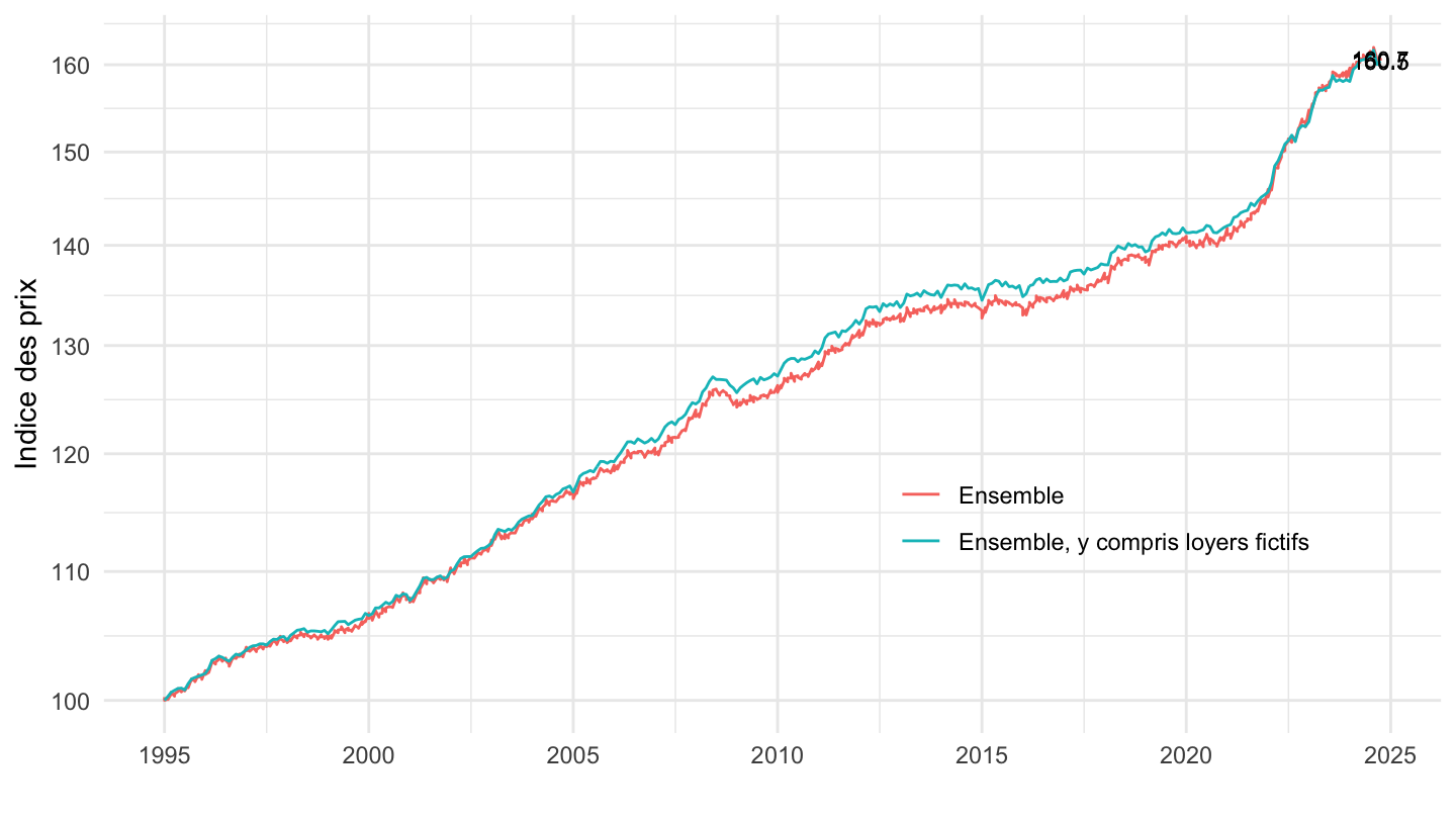
2008-
Code
`IPC-2015` %>%
  filter(INDICATEUR == "IPC",
         REF_AREA == "FE",
         PRIX_CONSO %in% c("00", "4035"),
         #PRIX_CONSO %in% c("00"),
         NATURE == "INDICE",
         FREQ == "M") %>%
  month_to_date %>%
  group_by(PRIX_CONSO) %>%
  mutate(OBS_VALUE = 100*OBS_VALUE / OBS_VALUE[date == as.Date("2008-01-01")]) %>%
  filter(date >= as.Date("2008-01-01")) %>%

  ggplot() + ylab("Indice des prix") + xlab("") + theme_minimal() +
  geom_line(aes(x = date, y = OBS_VALUE, color = Prix_conso)) +

  scale_x_date(breaks = seq(1920, 2100, 2) %>% paste0("-01-01") %>% as.Date,
               labels = date_format("%Y")) +
  theme(legend.position = c(0.75, 0.3),
        legend.title = element_blank()) +
  scale_y_log10(breaks = seq(0, 200, 2),
                     labels = dollar_format(accuracy = 1, prefix = "")) +
  geom_text_repel(data = . %>%
              filter(date == max(date)), aes(x = date, y = OBS_VALUE, label = round(OBS_VALUE, 1)), size = 3)
Categories
Par Deciles - INF-D1, D5-D6, D9-PLUS
Code
`IPC-2015` %>%
  filter(MENAGES_IPC %in% c("INF-D1", "D5-D6", "D9-PLUS")) %>%
  year_to_date %>%

  group_by(MENAGES_IPC) %>%
  arrange(date) %>%
  mutate(OBS_VALUE = 100*OBS_VALUE/OBS_VALUE[1]) %>%
  ggplot() + ylab("Indice des prix") + xlab("") + theme_minimal() +
  geom_line(aes(x = date, y = OBS_VALUE, color = Menages_ipc)) +

  scale_x_date(breaks = seq(1920, 2100, 2) %>% paste0("-01-01") %>% as.Date,
               labels = date_format("%Y")) +
  theme(legend.position = c(0.35, 0.9),
        legend.title = element_blank()) +
  scale_y_log10(breaks = seq(0, 200, 5),
                     labels = dollar_format(accuracy = 1, prefix = "")) +
  geom_text_repel(data = . %>%
              filter(date == max(date)), aes(x = date, y = OBS_VALUE, label = round(OBS_VALUE, 1)), size = 3)
Par CSP - Actif, Retraité, Cadre, Ouvrier
Code
`IPC-2015` %>%
  filter(MENAGES_IPC %in% c("ACTIF", "RETRAITE", "CADRE", "OUVRIER")) %>%
  year_to_date %>%

  group_by(MENAGES_IPC) %>%
  arrange(date) %>%
  mutate(OBS_VALUE = 100*OBS_VALUE/OBS_VALUE[1]) %>%
  ggplot() + ylab("Indice des prix") + xlab("") + theme_minimal() +
  geom_line(aes(x = date, y = OBS_VALUE, color = Menages_ipc)) +

  scale_x_date(breaks = seq(1920, 2100, 2) %>% paste0("-01-01") %>% as.Date,
               labels = date_format("%Y")) +
  theme(legend.position = c(0.35, 0.85),
        legend.title = element_blank()) +
  scale_y_log10(breaks = seq(0, 200, 5),
                     labels = dollar_format(accuracy = 1, prefix = "")) +
  geom_text_repel(data = . %>%
              filter(date == max(date)), aes(x = date, y = OBS_VALUE, label = round(OBS_VALUE, 1)), size = 3)
Par Age - 30-44, 45-59, 60-74
All
Code
`IPC-2015` %>%
  filter(MENAGES_IPC %in% c("MOINS-29", "30-44", "45-59", "60-74", "PLUS-75")) %>%
  year_to_date %>%

  group_by(MENAGES_IPC) %>%
  arrange(date) %>%
  mutate(OBS_VALUE = 100*OBS_VALUE/OBS_VALUE[1]) %>%
  ggplot() + ylab("Indice des prix") + xlab("") + theme_minimal() +
  geom_line(aes(x = date, y = OBS_VALUE, color = Menages_ipc)) +
  scale_color_manual(values = viridis(6)[1:5]) +
  scale_x_date(breaks = seq(1920, 2100, 2) %>% paste0("-01-01") %>% as.Date,
               labels = date_format("%Y")) +
  theme(legend.position = c(0.75, 0.3),
        legend.title = element_blank()) +
  scale_y_log10(breaks = seq(0, 200, 5),
                     labels = dollar_format(accuracy = 1, prefix = ""))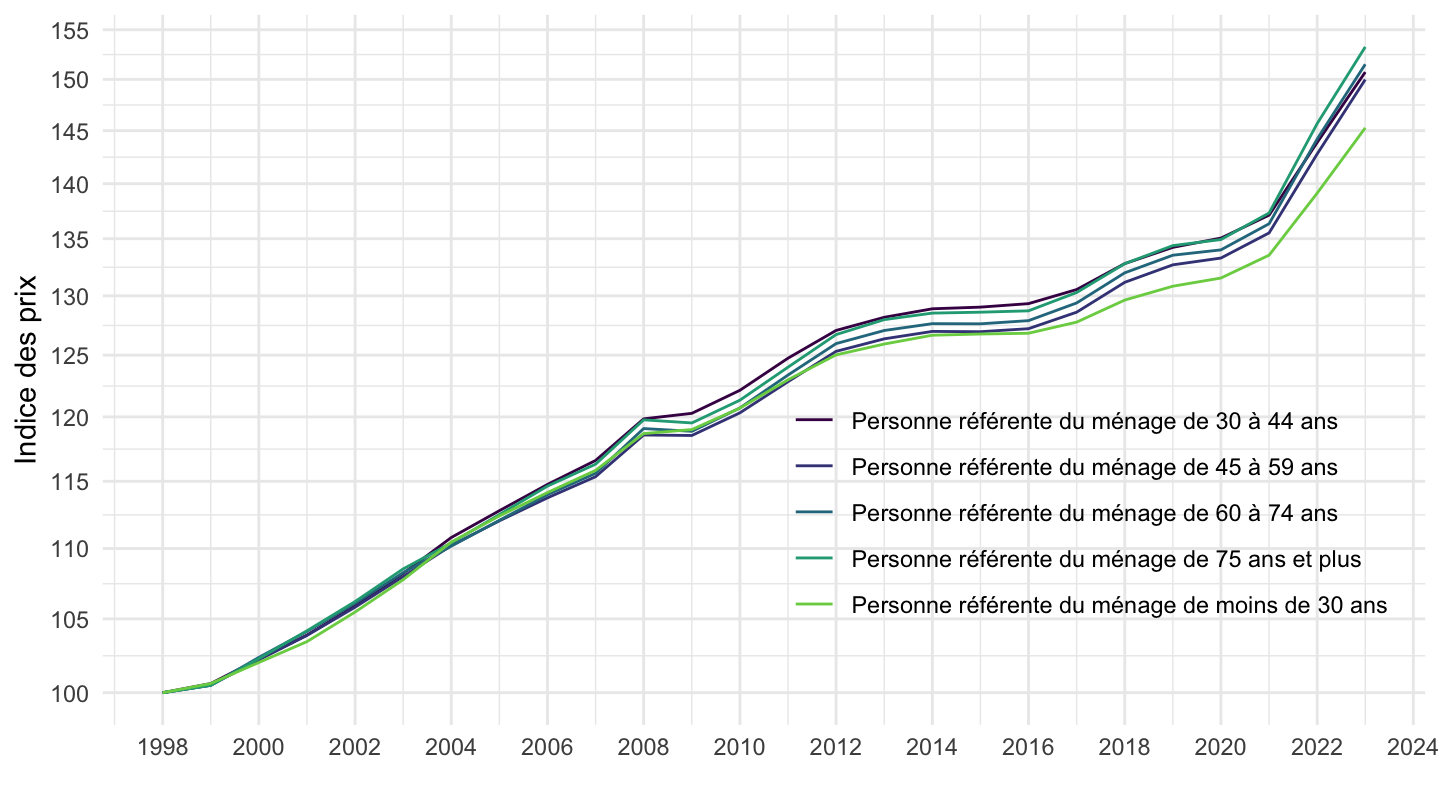
2008-
Code
`IPC-2015` %>%
  filter(MENAGES_IPC %in% c("MOINS-29", "ENSEMBLE", "45-59", "PLUS-75"),
         INDICATEUR == "IPC",
         PRIX_CONSO == "4035",
         NATURE == "INDICE",
         REF_AREA == "FM",
         FREQ == "A",
         COICOP2016 == "SO") %>%
  year_to_date %>%
  group_by(MENAGES_IPC) %>%
  mutate(OBS_VALUE = 100*OBS_VALUE / OBS_VALUE[date == as.Date("2008-01-01")]) %>%
  filter(date >= as.Date("2008-01-01")) %>%

  ggplot() + ylab("Indice des prix") + xlab("") + theme_minimal() +
  geom_line(aes(x = date, y = OBS_VALUE, color = Menages_ipc)) +

  scale_x_date(breaks = seq(1920, 2100, 1) %>% paste0("-01-01") %>% as.Date,
               labels = date_format("%Y")) +
  theme(legend.position = c(0.75, 0.3),
        legend.title = element_blank()) +
  scale_y_log10(breaks = seq(0, 200, 1),
                     labels = dollar_format(accuracy = 1, prefix = ""))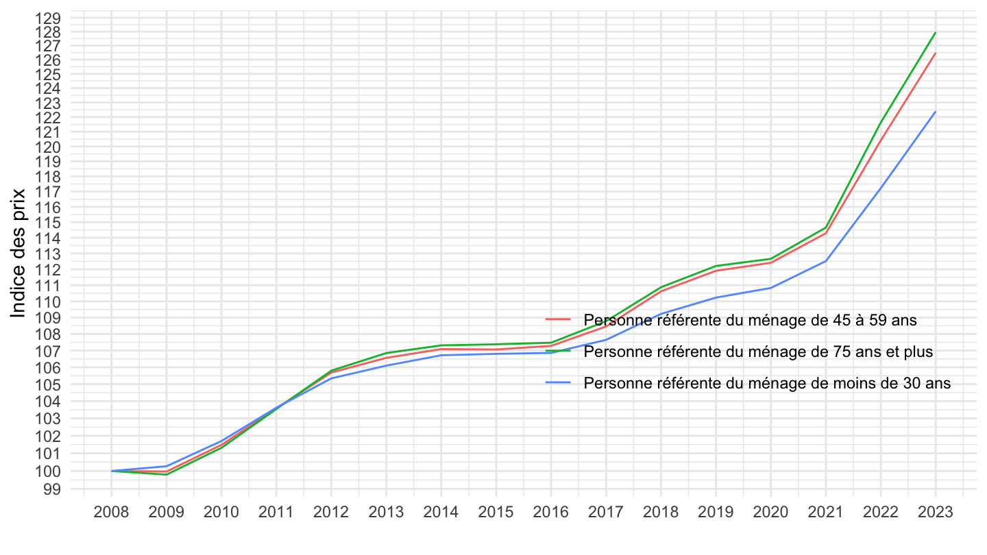
Locataire VS Propriétaire VS Accédant
Code
`IPC-2015` %>%
  filter(MENAGES_IPC %in% c("ACCES-PROPRIETE", "LOCATAIRE", "PROPRIETAIRE")) %>%
  year_to_date %>%

  group_by(MENAGES_IPC) %>%
  arrange(date) %>%
  mutate(OBS_VALUE = 100*OBS_VALUE/OBS_VALUE[1]) %>%
  ggplot() + ylab("Indice des prix") + xlab("") + theme_minimal() +
  geom_line(aes(x = date, y = OBS_VALUE, color = Menages_ipc, linetype = Menages_ipc)) +

  scale_x_date(breaks = seq(1920, 2100, 2) %>% paste0("-01-01") %>% as.Date,
               labels = date_format("%Y")) +
  theme(legend.position = c(0.75, 0.3),
        legend.title = element_blank()) +
  scale_y_log10(breaks = seq(0, 200, 5),
                     labels = dollar_format(accuracy = 1, prefix = ""))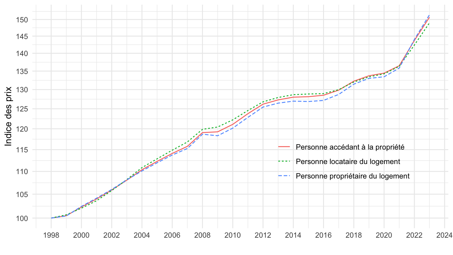
Cantines
1990-
Code
`IPC-2015` %>%
  filter(COICOP2016 %in% c("00", "1112"),
         REF_AREA == "FM",
         FREQ == "M") %>%
  month_to_date %>%

  filter(date >= as.Date("1990-01-01")) %>%
  group_by(COICOP2016) %>%
  arrange(date) %>%
  mutate(OBS_VALUE = 100*OBS_VALUE/OBS_VALUE[1]) %>%
  ggplot() + ylab("Indice des prix") + xlab("") + theme_minimal() +
  geom_line(aes(x = date, y = OBS_VALUE, color = Coicop2016)) +

  scale_x_date(breaks = seq(1920, 2100, 2) %>% paste0("-01-01") %>% as.Date,
               labels = date_format("%Y")) +
  theme(legend.position = c(0.25, 0.9),
        legend.title = element_blank()) +
  scale_y_log10(breaks = seq(0, 200, 5),
                     labels = dollar_format(accuracy = 1, prefix = ""))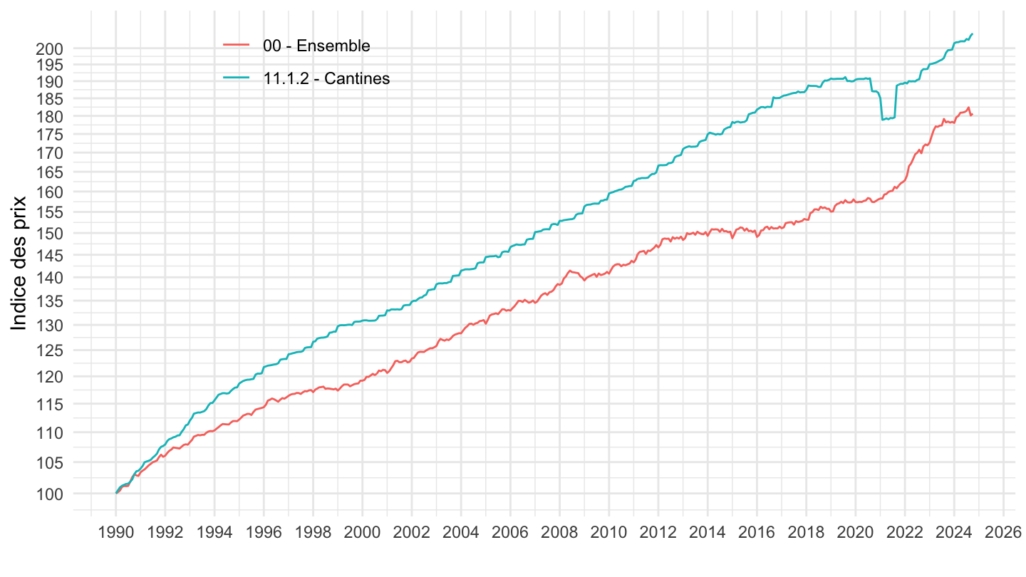
2000-
Code
`IPC-2015` %>%
  filter(COICOP2016 %in% c("00", "1112"),
         REF_AREA == "FM",
         FREQ == "M") %>%
  month_to_date %>%

  filter(date >= as.Date("2000-01-01")) %>%
  group_by(COICOP2016) %>%
  arrange(date) %>%
  mutate(OBS_VALUE = 100*OBS_VALUE/OBS_VALUE[1]) %>%
  ggplot() + ylab("Indice des prix") + xlab("") + theme_minimal() +
  geom_line(aes(x = date, y = OBS_VALUE, color = Coicop2016)) +

  scale_x_date(breaks = seq(1920, 2100, 2) %>% paste0("-01-01") %>% as.Date,
               labels = date_format("%Y")) +
  theme(legend.position = c(0.25, 0.9),
        legend.title = element_blank()) +
  scale_y_log10(breaks = seq(0, 200, 5),
                     labels = dollar_format(accuracy = 1, prefix = ""))
2010-
Code
`IPC-2015` %>%
  filter(COICOP2016 %in% c("00", "1112"),
         REF_AREA == "FM",
         FREQ == "M") %>%
  month_to_date %>%

  filter(date >= as.Date("2010-01-01")) %>%
  group_by(COICOP2016) %>%
  arrange(date) %>%
  mutate(OBS_VALUE = 100*OBS_VALUE/OBS_VALUE[1]) %>%
  ggplot() + ylab("Indice des prix") + xlab("") + theme_minimal() +
  geom_line(aes(x = date, y = OBS_VALUE, color = Coicop2016)) +

  scale_x_date(breaks = seq(1920, 2100, 2) %>% paste0("-01-01") %>% as.Date,
               labels = date_format("%Y")) +
  theme(legend.position = c(0.25, 0.9),
        legend.title = element_blank()) +
  scale_y_log10(breaks = seq(0, 200, 5),
                     labels = dollar_format(accuracy = 1, prefix = ""))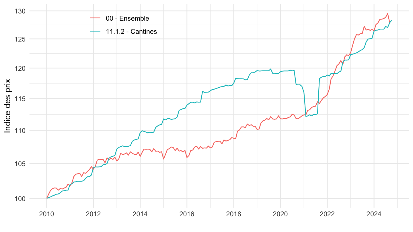
Scolaire, Universitaire VS Entreprise ou Admin.
Code
`IPC-2015` %>%
  filter(COICOP2016 %in% c("111202", "111201"),
         NATURE == "INDICE") %>%
  year_to_date %>%
  arrange(desc(date)) %>%

  group_by(COICOP2016) %>%
  arrange(date) %>%
  mutate(OBS_VALUE = 100*OBS_VALUE/OBS_VALUE[1]) %>%
  ggplot() + ylab("Indice des prix") + xlab("") + theme_minimal() +
  geom_line(aes(x = date, y = OBS_VALUE, color = Coicop2016)) +

  scale_x_date(breaks = seq(1920, 2100, 5) %>% paste0("-01-01") %>% as.Date,
               labels = date_format("%Y")) +
  theme(legend.position = c(0.35, 0.9),
        legend.title = element_blank()) +
  scale_y_log10(breaks = seq(0, 200, 5),
                     labels = dollar_format(accuracy = 1, prefix = ""))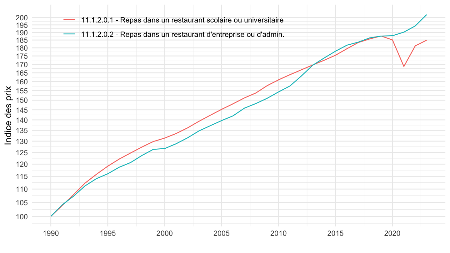
Assurance santé
1990-
Code
`IPC-2015` %>%
  filter(COICOP2016 %in% c("00", "12532", "1253"),
         REF_AREA == "FM",
         FREQ == "M") %>%
  month_to_date %>%

  filter(date >= as.Date("1990-01-01")) %>%
  group_by(COICOP2016) %>%
  arrange(date) %>%
  mutate(OBS_VALUE = 100*OBS_VALUE/OBS_VALUE[1]) %>%
  ggplot() + ylab("Indice des prix") + xlab("") + theme_minimal() +
  geom_line(aes(x = date, y = OBS_VALUE, color = Coicop2016)) +

  scale_x_date(breaks = seq(1920, 2100, 2) %>% paste0("-01-01") %>% as.Date,
               labels = date_format("%Y")) +
  theme(legend.position = c(0.25, 0.9),
        legend.title = element_blank()) +
  scale_y_log10(breaks = seq(0, 200, 5),
                     labels = dollar_format(accuracy = 1, prefix = ""))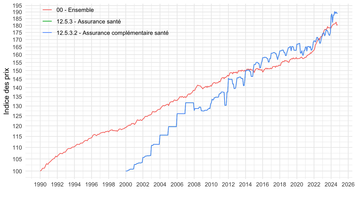
2000-
Code
`IPC-2015` %>%
  filter(COICOP2016 %in% c("00", "12532", "1253"),
         REF_AREA == "FM",
         FREQ == "M") %>%
  month_to_date %>%

  filter(date >= as.Date("2000-01-01")) %>%
  group_by(COICOP2016) %>%
  arrange(date) %>%
  mutate(OBS_VALUE = 100*OBS_VALUE/OBS_VALUE[1]) %>%
  ggplot() + ylab("Indice des prix") + xlab("") + theme_minimal() +
  geom_line(aes(x = date, y = OBS_VALUE, color = Coicop2016)) +

  scale_x_date(breaks = seq(1920, 2100, 2) %>% paste0("-01-01") %>% as.Date,
               labels = date_format("%Y")) +
  theme(legend.position = c(0.25, 0.9),
        legend.title = element_blank()) +
  scale_y_log10(breaks = seq(0, 200, 5),
                     labels = dollar_format(accuracy = 1, prefix = ""))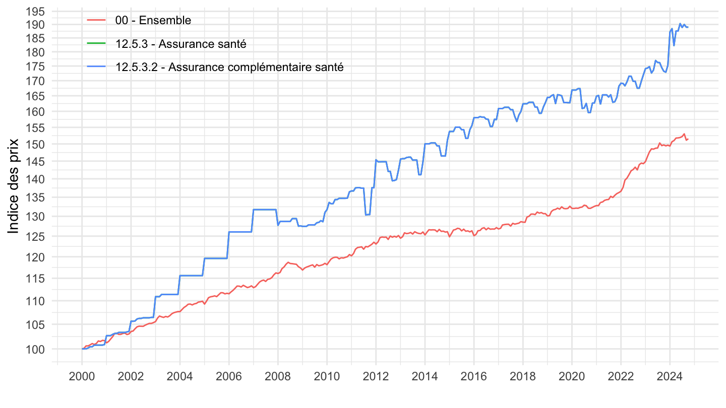
2010-
Code
`IPC-2015` %>%
  filter(COICOP2016 %in% c("00", "12532"),
         REF_AREA == "FM",
         FREQ == "M") %>%
  month_to_date %>%

  filter(date >= as.Date("2010-01-01")) %>%
  group_by(COICOP2016) %>%
  arrange(date) %>%
  mutate(OBS_VALUE = 100*OBS_VALUE/OBS_VALUE[1]) %>%
  ggplot() + ylab("Indice des prix") + xlab("") + theme_minimal() +
  geom_line(aes(x = date, y = OBS_VALUE, color = Coicop2016)) +

  scale_x_date(breaks = seq(1920, 2100, 2) %>% paste0("-01-01") %>% as.Date,
               labels = date_format("%Y")) +
  theme(legend.position = c(0.25, 0.9),
        legend.title = element_blank()) +
  scale_y_log10(breaks = seq(0, 200, 5),
                     labels = dollar_format(accuracy = 1, prefix = ""))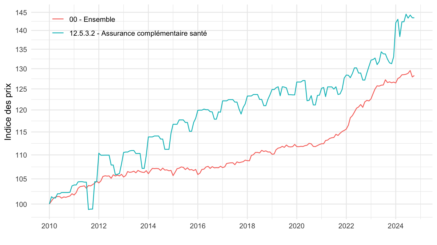
2-digit
Boissons Alcoolisées, Logement, Restaurants et hôtels
All
Code
`IPC-2015` %>%
  filter(COICOP2016 %in% c("00", "02", "11", "04"),
         REF_AREA == "FM",
         FREQ == "M") %>%
  month_to_date %>%

  group_by(COICOP2016) %>%
  arrange(date) %>%
  mutate(OBS_VALUE = 100*OBS_VALUE/OBS_VALUE[1]) %>%
  ggplot() + ylab("Indice des prix") + xlab("") + theme_minimal() +
  geom_line(aes(x = date, y = OBS_VALUE, color = Coicop2016)) +

  scale_x_date(breaks = seq(1920, 2100, 2) %>% paste0("-01-01") %>% as.Date,
               labels = date_format("%Y")) +
  theme(legend.position = c(0.3, 0.85),
        legend.title = element_blank()) +
  scale_y_log10(breaks = c(100, 120, 150, 200, 220, 250, 300, 400, 500),
                     labels = dollar_format(accuracy = 1, prefix = ""))
Glissement sur 2 ans
Code
`IPC-2015` %>%
  filter(COICOP2016 %in% c("00", "02", "11", "04"),
         REF_AREA == "FM",
         FREQ == "M") %>%
  month_to_date %>%
  filter(date >= max(date) - years(2)) %>%

  group_by(COICOP2016) %>%
  arrange(date) %>%
  mutate(OBS_VALUE = 100*OBS_VALUE/OBS_VALUE[1]) %>%
  ggplot + geom_line(aes(x = date, y = OBS_VALUE, color = Coicop2016)) +
  theme_minimal() + xlab("") + ylab("") +
  scale_x_date(breaks = "1 month",
               labels = date_format("%b %Y")) +
  theme(legend.position = c(0.28, 0.87),
        legend.title = element_blank(),
        axis.text.x = element_text(angle = 45, vjust = 0.5, hjust=1)) +
  scale_y_log10(breaks = seq(0, 200, 1),
                     labels = dollar_format(accuracy = 1, prefix = "")) +
  geom_text_repel(aes(x = date, y = OBS_VALUE, label = round(OBS_VALUE, 1)),
                  fontface ="plain", color = "black", size = 3)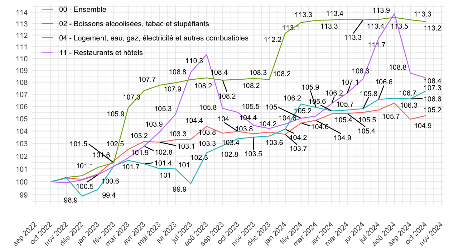
Transports, Enseignement, B&S Divers
Tous
Code
`IPC-2015` %>%
  filter(COICOP2016 %in% c("00", "10", "07", "12"),
         REF_AREA == "FM",
         FREQ == "M") %>%
  month_to_date %>%

  group_by(COICOP2016) %>%
  arrange(date) %>%
  mutate(OBS_VALUE = 100*OBS_VALUE/OBS_VALUE[1]) %>%
  ggplot() + ylab("Indice des prix") + xlab("") + theme_minimal() +
  geom_line(aes(x = date, y = OBS_VALUE, color = Coicop2016)) +

  scale_x_date(breaks = seq(1920, 2100, 2) %>% paste0("-01-01") %>% as.Date,
               labels = date_format("%Y")) +
  theme(legend.position = c(0.3, 0.85),
        legend.title = element_blank()) +
  scale_y_log10(breaks = seq(100, 300, 10),
                     labels = dollar_format(accuracy = 1, prefix = ""))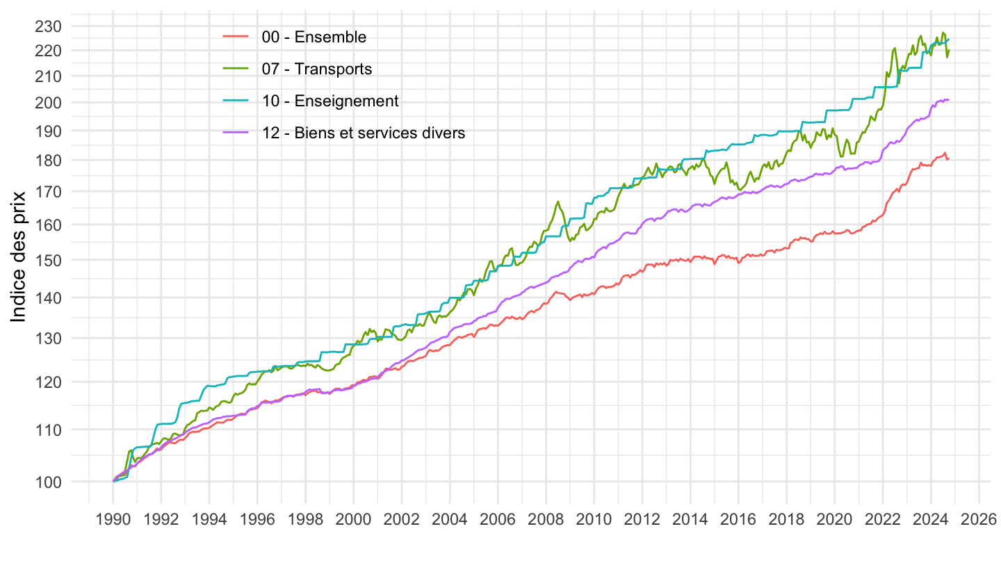
Glissement sur 2 ans
Code
`IPC-2015` %>%
  filter(COICOP2016 %in% c("00", "10", "07", "12"),
         REF_AREA == "FM",
         FREQ == "M") %>%
  month_to_date %>%
  filter(date >= max(date) - years(2)) %>%

  group_by(COICOP2016) %>%
  arrange(date) %>%
  mutate(OBS_VALUE = 100*OBS_VALUE/OBS_VALUE[1]) %>%
  ggplot + geom_line(aes(x = date, y = OBS_VALUE, color = Coicop2016)) +
  theme_minimal() + xlab("") + ylab("") +
  scale_x_date(breaks = "1 month",
               labels = date_format("%b %Y")) +
  theme(legend.position = c(0.18, 0.87),
        legend.title = element_blank(),
        axis.text.x = element_text(angle = 45, vjust = 0.5, hjust=1)) +
  scale_y_log10(breaks = seq(0, 200, 2),
                     labels = dollar_format(accuracy = 1, prefix = "")) +
  geom_text_repel(aes(x = date, y = OBS_VALUE, label = round(OBS_VALUE, 1)),
                  fontface ="plain", color = "black", size = 3)
Alimentation, Habillement, Meubles
Tous
Code
`IPC-2015` %>%
  filter(COICOP2016 %in% c("00", "05", "01", "03"),
         REF_AREA == "FM",
         FREQ == "M") %>%
  month_to_date %>%

  group_by(COICOP2016) %>%
  arrange(date) %>%
  mutate(OBS_VALUE = 100*OBS_VALUE/OBS_VALUE[1]) %>%
  ggplot() + ylab("Indice des prix") + xlab("") + theme_minimal() +
  geom_line(aes(x = date, y = OBS_VALUE, color = Coicop2016)) +

  scale_x_date(breaks = seq(1920, 2100, 2) %>% paste0("-01-01") %>% as.Date,
               labels = date_format("%Y")) +
  theme(legend.position = c(0.35, 0.85),
        legend.title = element_blank()) +
  scale_y_log10(breaks = seq(100, 300, 10),
                     labels = dollar_format(accuracy = 1, prefix = ""))
Glissement sur 2 ans
Code
`IPC-2015` %>%
  filter(COICOP2016 %in% c("00", "05", "01", "03"),
         REF_AREA == "FM",
         FREQ == "M") %>%
  month_to_date %>%
  filter(date >= max(date) - years(2)) %>%

  group_by(COICOP2016) %>%
  arrange(date) %>%
  mutate(OBS_VALUE = 100*OBS_VALUE/OBS_VALUE[1]) %>%
  ggplot + geom_line(aes(x = date, y = OBS_VALUE, color = Coicop2016)) +
  theme_minimal() + xlab("") + ylab("") +
  scale_x_date(breaks = "1 month",
               labels = date_format("%b %Y")) +
  theme(legend.position = c(0.28, 0.87),
        legend.title = element_blank(),
        axis.text.x = element_text(angle = 45, vjust = 0.5, hjust=1)) +
  scale_y_log10(breaks = seq(0, 200, 2),
                     labels = dollar_format(accuracy = 1, prefix = "")) +
  geom_text_repel(aes(x = date, y = OBS_VALUE, label = round(OBS_VALUE, 1)),
                  fontface ="plain", color = "black", size = 3)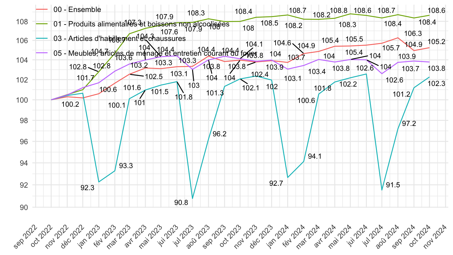
Santé, Communications, Loisirs
Tous
Code
`IPC-2015` %>%
  filter(COICOP2016 %in% c("00", "06", "09", "08"),
         REF_AREA == "FM",
         FREQ == "M") %>%
  month_to_date %>%

  group_by(COICOP2016) %>%
  arrange(date) %>%
  mutate(OBS_VALUE = 100*OBS_VALUE/OBS_VALUE[1]) %>%
  ggplot() + ylab("Indice des prix") + xlab("") + theme_minimal() +
  geom_line(aes(x = date, y = OBS_VALUE, color = Coicop2016)) +

  scale_x_date(breaks = seq(1920, 2100, 2) %>% paste0("-01-01") %>% as.Date,
               labels = date_format("%Y")) +
  theme(legend.position = c(0.2, 0.2),
        legend.title = element_blank()) +
  scale_y_log10(breaks = seq(10, 300, 10),
                     labels = dollar_format(accuracy = 1, prefix = ""))
1996-
Code
`IPC-2015` %>%
  filter(COICOP2016 %in% c("00", "06", "09", "08"),
         REF_AREA == "FM",
         FREQ == "M") %>%
  month_to_date %>%
  filter(date >= as.Date("1996-01-01")) %>%

  group_by(COICOP2016) %>%
  arrange(date) %>%
  mutate(OBS_VALUE = 100*OBS_VALUE/OBS_VALUE[1]) %>%
  ggplot() + ylab("Indice des prix") + xlab("") + theme_minimal() +
  geom_line(aes(x = date, y = OBS_VALUE, color = Coicop2016)) +

  scale_x_date(breaks = seq(1920, 2100, 2) %>% paste0("-01-01") %>% as.Date,
               labels = date_format("%Y")) +
  theme(legend.position = c(0.2, 0.2),
        legend.title = element_blank()) +
  scale_y_log10(breaks = seq(10, 300, 10),
                     labels = dollar_format(accuracy = 1, prefix = ""))
2000-
Code
`IPC-2015` %>%
  filter(COICOP2016 %in% c("00", "06", "09", "08"),
         REF_AREA == "FM",
         FREQ == "M") %>%
  month_to_date %>%
  filter(date >= as.Date("2000-01-01")) %>%

  group_by(COICOP2016) %>%
  arrange(date) %>%
  mutate(OBS_VALUE = 100*OBS_VALUE/OBS_VALUE[1]) %>%
  ggplot() + ylab("Indice des prix") + xlab("") + theme_minimal() +
  geom_line(aes(x = date, y = OBS_VALUE, color = Coicop2016)) +

  scale_x_date(breaks = seq(1920, 2100, 2) %>% paste0("-01-01") %>% as.Date,
               labels = date_format("%Y")) +
  theme(legend.position = c(0.18, 0.22),
        legend.title = element_blank()) +
  scale_y_log10(breaks = seq(10, 300, 10),
                     labels = dollar_format(accuracy = 1, prefix = ""))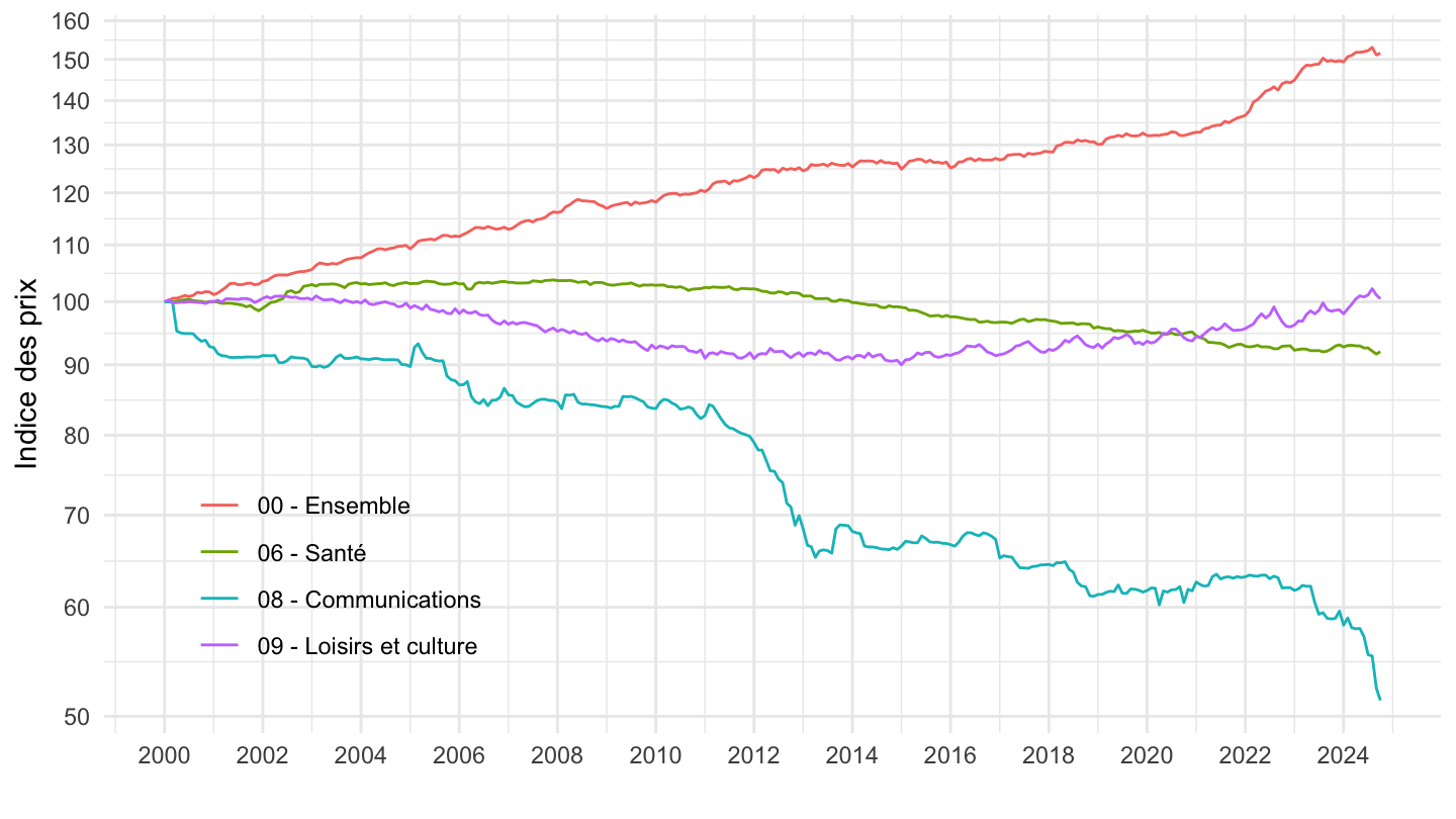
Glissement sur 2 ans
Code
`IPC-2015` %>%
  filter(COICOP2016 %in% c("00", "06", "09", "08"),
         REF_AREA == "FM",
         FREQ == "M") %>%
  month_to_date %>%
  filter(date >= max(date) - years(2)) %>%

  group_by(COICOP2016) %>%
  arrange(date) %>%
  mutate(OBS_VALUE = 100*OBS_VALUE/OBS_VALUE[1]) %>%
  ggplot + geom_line(aes(x = date, y = OBS_VALUE, color = Coicop2016)) +
  theme_minimal() + xlab("") + ylab("") +
  scale_x_date(breaks = "1 month",
               labels = date_format("%b %Y")) +
  theme(legend.position = c(0.28, 0.87),
        legend.title = element_blank(),
        axis.text.x = element_text(angle = 45, vjust = 0.5, hjust=1)) +
  scale_y_log10(breaks = seq(0, 200, 2),
                     labels = dollar_format(accuracy = 1, prefix = "")) +
  geom_text_repel(aes(x = date, y = OBS_VALUE, label = round(OBS_VALUE, 1)),
                  fontface ="plain", color = "black", size = 3)
Comparer l’IPC et le déflateur de la consommation
Revenu primaire au RDB
Code
ig_b("insee", "FPS2021", "revenu-primaire-RDB")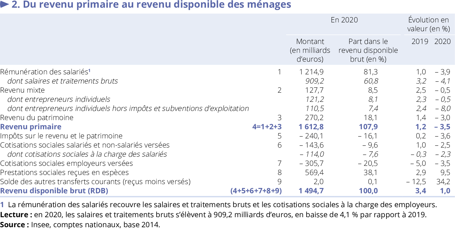
Déflateur consommation finale des ménages
Code
ig_b("insee", "FPS2021", "depense-consommation-finale-menages")