
Last observation: Q1 2026 (N = 69) · mars 2026 (N = 91) · 2025 (N = 2479)
First observation: 1914 (N = 1) · janv. 1914 (N = 1) · Q1 1914 (N = 1)
Last data update: 02 août 2026, 09:03
Last compile: 19 oct. 2026, 01:47
PRICES_CPI |>
  left_join(PRICES_CPI_var$SUBJECT, by = "SUBJECT") |>
  group_by(SUBJECT, Subject, MEASURE, FREQUENCY) |>
  summarise(Nobs = sum(!is.na(obsValue))) |>
  arrange(-Nobs) |>
print_table_conditional()PRICES_CPI |>
filter(MEASURE == "IXOB",
FREQUENCY == "A") |>
left_join(PRICES_CPI_var$SUBJECT, by = "SUBJECT") |>
group_by(SUBJECT, Subject) |>
summarise(nobs = sum(!is.na(obsValue))) |>
arrange(-nobs) |>
print_table_conditional()| SUBJECT | Subject | nobs |
|---|---|---|
| CPALTT01 | CPI: 01-12 - All items | 2875 |
| CP010000 | CPI: 01 - Food and non-Alcoholic beverages | 2224 |
| PWCP0100 | CPI weights: 01 - Food and non-Alcoholic beverages | 2224 |
| CPGREN01 | CPI: Energy | 2047 |
| CPGRLE01 | CPI: All items non-food non-energy | 2015 |
| CP040100 | CPI: 04.1 - CPI Actual rentals for housing | 1422 |
| PWCP0410 | CPI weights: 04.1 - Actual Rentals for Housing | 1422 |
| CP080000 | CPI: 08 - Communication | 1245 |
| PWCP0400 | CPI weights: 04 - Housing, water, electricity, gas and other fuels | 1245 |
| PWCP0800 | CPI weights: 08 - Communication | 1245 |
| CP030000 | CPI: 03 - Clothing and footwear | 1206 |
| PWCP0300 | CPI weights: 03 - Clothing and footwear | 1206 |
| PWCP0500 | CPI weights: 05 - Furnishings, household equipment and routine household maintenance | 1206 |
| PWCP0900 | CPI weights: 09 - Recreation and culture | 1206 |
| CP110000 | CPI: 11 - Restaurants and hotels | 1197 |
| PWCP1100 | CPI weights: 11 - Restaurants and hotels | 1197 |
| PWCP1000 | CPI weights: 10 - Education | 1191 |
| PWCP1200 | CPI weights: 12 - Miscellaneous goods and services | 1191 |
| CP020000 | CPI: 02 - Alcoholic beverages, tobacco and narcotics | 1167 |
| PWCP0200 | CPI weights: 02 - Alcoholic beverages, tobacco and narcotics | 1167 |
| PWCP0600 | CPI weights: 06 - Health | 1150 |
| PWCP0700 | CPI weights: 07 - Transport | 1113 |
| CPHPTT01 | HICP: All items | 946 |
| CPGRHO01 | CPI: Housing | 921 |
| CPGRLH01 | CPI: Services less housing | 639 |
| CP040200 | CPI: 04.2 - CPI Imputed rentals for housing | 619 |
| PWCP0420 | CPI weights: 04.2 - Imputed Rentals for Housing | 619 |
i_g("bib/oecd/PRICES_CPI_COICOP.png")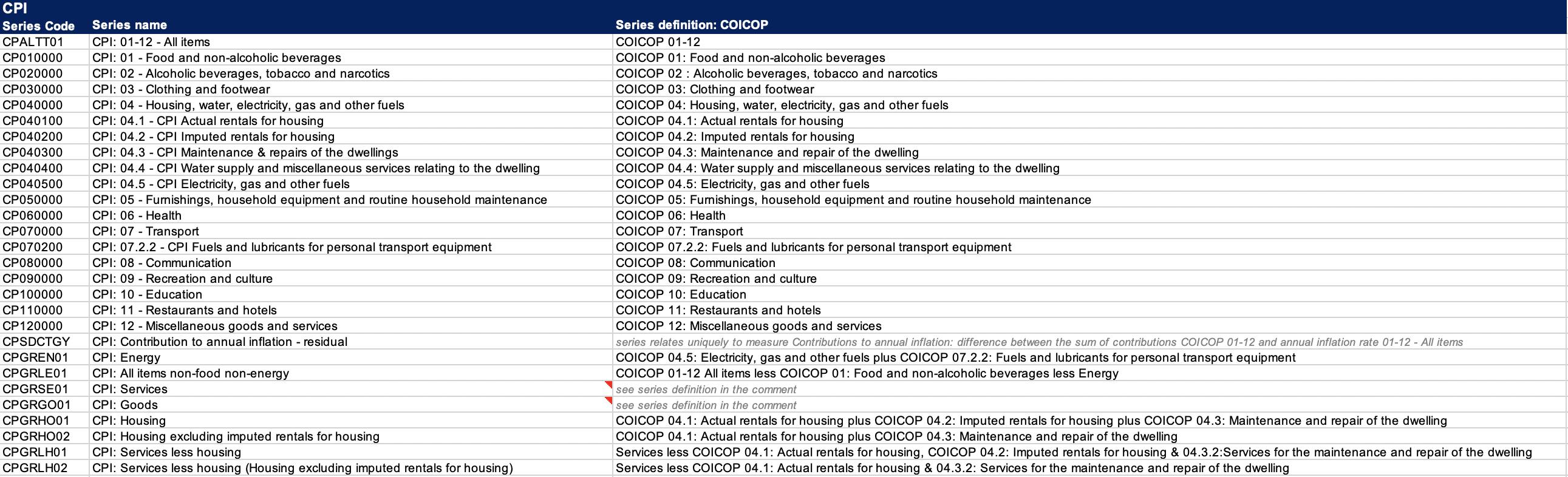
i_g("bib/oecd/PRICES_CPI_weights.png")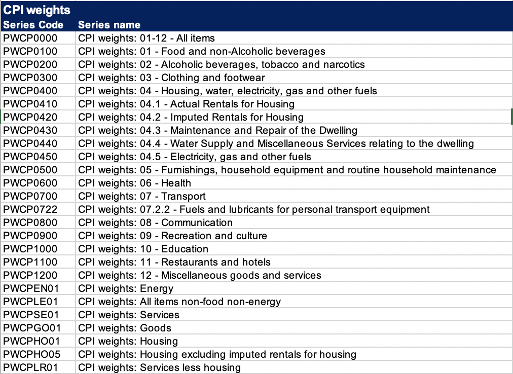
i_g("bib/oecd/PRICES_CPI_HICP.png")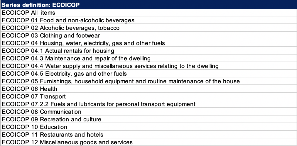
PRICES_CPI |>
  left_join(PRICES_CPI_var$SUBJECT, by = "SUBJECT") |>
  group_by(SUBJECT, Subject) |>
  summarise(Nobs = sum(!is.na(obsValue))) |>
  arrange(-Nobs) |>
print_table_conditional()| SUBJECT | Subject | Nobs |
|---|---|---|
| CPALTT01 | CPI: 01-12 - All items | 144121 |
| CP010000 | CPI: 01 - Food and non-Alcoholic beverages | 120605 |
| PWCP0100 | CPI weights: 01 - Food and non-Alcoholic beverages | 120605 |
| CPGREN01 | CPI: Energy | 106452 |
| CPGRLE01 | CPI: All items non-food non-energy | 106075 |
| CP040100 | CPI: 04.1 - CPI Actual rentals for housing | 75914 |
| PWCP0410 | CPI weights: 04.1 - Actual Rentals for Housing | 75914 |
| PWCP0400 | CPI weights: 04 - Housing, water, electricity, gas and other fuels | 68348 |
| CP080000 | CPI: 08 - Communication | 68141 |
| PWCP0800 | CPI weights: 08 - Communication | 68141 |
| PWCP0500 | CPI weights: 05 - Furnishings, household equipment and routine household maintenance | 67760 |
| PWCP0900 | CPI weights: 09 - Recreation and culture | 67760 |
| CP110000 | CPI: 11 - Restaurants and hotels | 67311 |
| PWCP1100 | CPI weights: 11 - Restaurants and hotels | 67311 |
| PWCP0600 | CPI weights: 06 - Health | 67123 |
| PWCP1200 | CPI weights: 12 - Miscellaneous goods and services | 66995 |
| CP030000 | CPI: 03 - Clothing and footwear | 66857 |
| PWCP0300 | CPI weights: 03 - Clothing and footwear | 66857 |
| CP020000 | CPI: 02 - Alcoholic beverages, tobacco and narcotics | 65783 |
| PWCP0200 | CPI weights: 02 - Alcoholic beverages, tobacco and narcotics | 65783 |
| PWCP1000 | CPI weights: 10 - Education | 65702 |
| PWCP0700 | CPI weights: 07 - Transport | 64406 |
| CPGRHO01 | CPI: Housing | 47544 |
| CPHPTT01 | HICP: All items | 36166 |
| CPGRLH01 | CPI: Services less housing | 32069 |
| CP040200 | CPI: 04.2 - CPI Imputed rentals for housing | 32064 |
| PWCP0420 | CPI weights: 04.2 - Imputed Rentals for Housing | 32064 |
PRICES_CPI |>
  filter(!is.na(obsValue)) |>
  group_by(obsTime) |>
  summarise(Nobs = n()) |>
  arrange(desc(obsTime)) |>
print_table_conditional()# OECD stopped publishing the US contribution-to-inflation decomposition for
# energy (CPGREN01) and core (CPGRLE01) after 2023-12, while the headline / food
# / rents contributions and the plain YoY energy rate (GY) still run to the
# present. Fill the missing energy contribution with w * YoY, where w is the
# energy CPI weight implied by the overlap period, and let the residual (Total
# less Energy, Food and Rents) absorb the small reconciliation gap so the stack
# keeps summing to headline inflation (CPALTT01).
us_nrg_gy <- PRICES_CPI |>
filter(MEASURE == "GY", LOCATION == "USA", SUBJECT == "CPGREN01") |>
month_to_date() |>
select(date, nrg_gy = obsValue)
us_ctgy <- PRICES_CPI |>
filter(MEASURE == "CTGY",
LOCATION %in% c("USA"),
SUBJECT %in% c("CPGRLE01", "CPGREN01", "CP010000", "CP020000",
"CPALTT01", "CP040100", "CP040200")) |>
month_to_date() |>
filter(date >= as.Date("2020-01-01")) |>
select(date, obsValue, SUBJECT) |>
spread(SUBJECT, obsValue) |>
left_join(us_nrg_gy, by = "date") |>
mutate(CPGREN01 = coalesce(CPGREN01,
median(CPGREN01 / nrg_gy, na.rm = TRUE) * nrg_gy))
line_US <- us_ctgy |>
transmute(date, `Total inflation` = CPALTT01,
`Core inflation` = CPALTT01 - (CP010000 + CP020000) - CPGREN01) |>
gather(Coicop, values, -date) |>
filter(!is.na(values)) |>
mutate(Coicop = factor(Coicop, levels = c("Total inflation", "Core inflation")),
Geo = "US")
bars_US <- us_ctgy |>
transmute(date,
FOOD = CP010000 + CP020000,
NRG = CPGREN01,
RENTS = CP040100+CP040200,
TOT_X_NRG_FOOD_RENTS = CPALTT01-FOOD-NRG-RENTS) |>
filter(!is.na(TOT_X_NRG_FOOD_RENTS)) |>
gather(coicop, values, -date) |>
# CP070200, CP040500, CP010000
# CPGRSE01, CPGRGO01
mutate(Coicop = factor(coicop, levels = c("FOOD", "NRG", "RENTS", "TOT_X_NRG_FOOD_RENTS"),
labels = c("Food", "Energy", "Rents",
"Total less Energy, Food and Rents")),
Geo = "US")
bars_US |>
ggplot(aes(x = date, y = values/100)) +
geom_col(aes(fill = Coicop), alpha = 1) +
geom_line(data = line_US, aes(linetype = Coicop), size = 1.2) +
theme_minimal() + xlab("") + ylab("Contributions to inflation") +
scale_fill_manual(values = c("forestgreen","orange", "grey", "blue")) +
scale_x_date(breaks ="3 months",
labels = date_format("%b %Y")) +
scale_y_continuous(breaks = 0.01*seq(-10, 30, 1),
labels = percent_format(accuracy = 1)) +
theme(legend.position = "top",
legend.title = element_blank(),
axis.text.x = element_text(angle = 45, vjust = 1, hjust = 1)) +
guides(fill=guide_legend(nrow=2))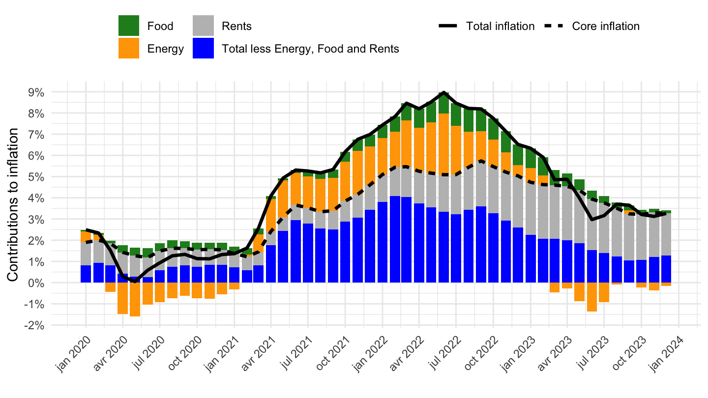
load_data("eurostat/prc_hicp_ctrb.RData")
line_EU <- prc_hicp_ctrb |>
  filter(coicop %in% c("NRG", "FOOD", "CP01", "CP02", "CP03", "CP04", "CP05", "CP06",
                       "CP07", "CP08", "CP09", "CP10", "CP11", "CP12", "CP041")) %>%
  mutate(date = gsub("M", "-", time) |> paste0("-01") |> as.Date()) |>
  filter(date >= as.Date("2020-01-01")) |>
  select(date, values, coicop) |>
  spread(coicop, values) |>
  transmute(date,
            `Total inflation` = CP01+CP02+CP03+CP04+CP05+CP06+CP07+CP08+CP09+CP10+CP11+CP12,
            FOOD,
            NRG,
            `Core inflation` = `Total inflation`-FOOD-NRG) |>
  select(date, `Total inflation`, `Core inflation`) |>
  gather(Coicop, values, -date) |>
  mutate(Coicop = factor(Coicop, levels = c("Total inflation", "Core inflation")),
         Geo = "Euro area")

bars_EU <- prc_hicp_ctrb |>
  filter(coicop %in% c("NRG", "FOOD", "CP01", "CP02", "CP03", "CP04", "CP05", "CP06",
                       "CP07", "CP08", "CP09", "CP10", "CP11", "CP12", "CP041")) %>%
  mutate(date = gsub("M", "-", time) |> paste0("-01") |> as.Date()) |>
  filter(date >= as.Date("2020-01-01")) |>
  select(date, values, coicop) |>
  spread(coicop, values) |>
  transmute(date,
            FOOD,
            NRG,
            RENTS = CP041,
            `Total inflation` = CP01+CP02+CP03+CP04+CP05+CP06+CP07+CP08+CP09+CP10+CP11+CP12,
            TOT_X_NRG_FOOD_RENTS = `Total inflation`-FOOD-NRG-RENTS) |>
  select(-`Total inflation`) |>
  gather(coicop, values, -date) |>
  # CP070200, CP040500, CP010000
  # CPGRSE01, CPGRGO01
  mutate(Coicop = factor(coicop, levels = c("FOOD", "NRG", "RENTS", "TOT_X_NRG_FOOD_RENTS"),
                         labels = c("Food", "Energy", "Rents",
                                    "Total less Energy, Food and Rents")),
         Geo = "Euro area")

bars_EU |>
  ggplot(aes(x = date, y = values/100)) +
  geom_col(aes(fill = Coicop), alpha = 1) +
  geom_line(data = line_EU, aes(linetype = Coicop), size = 1.2) +
  theme_minimal() + xlab("") + ylab("Contributions to inflation") +
  scale_fill_manual(values = c("forestgreen","orange", "grey", "blue")) +
  scale_x_date(breaks ="3 months",
               labels = date_format("%b %Y")) +
  scale_y_continuous(breaks = 0.01*seq(-10, 30, 1),
                     labels = percent_format(accuracy = 1)) +
  theme(legend.position = "top",
        legend.title = element_blank(),
        axis.text.x = element_text(angle = 45, vjust = 1, hjust = 1)) +
  guides(fill=guide_legend(nrow=2))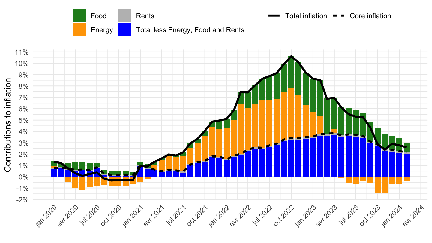
bars_EU |>
  bind_rows(bars_US) |>
  ggplot(aes(x = date, y = values/100)) +
  geom_col(aes(fill = Coicop), alpha = 1) +
  geom_line(data = line_EU |> bind_rows(line_US), aes(linetype = Coicop), size = 1.2) +
  theme_minimal() + xlab("") + ylab("Contributions to inflation") +
  scale_fill_manual(values = c("forestgreen","orange", "grey", "blue")) +
  scale_x_date(breaks ="6 months",
               labels = date_format("%b %Y"),
               expand = expansion(mult = 0.02)) +
  scale_y_continuous(breaks = 0.01*seq(-10, 30, 1),
                     labels = percent_format(accuracy = 1)) +
  theme(legend.position = "top",
        legend.title = element_blank(),
        axis.text.x = element_text(angle = 45, vjust = 1, hjust = 1)) +
  guides(fill=guide_legend(nrow=2)) +
  facet_wrap(~ Geo, scales = "free_x")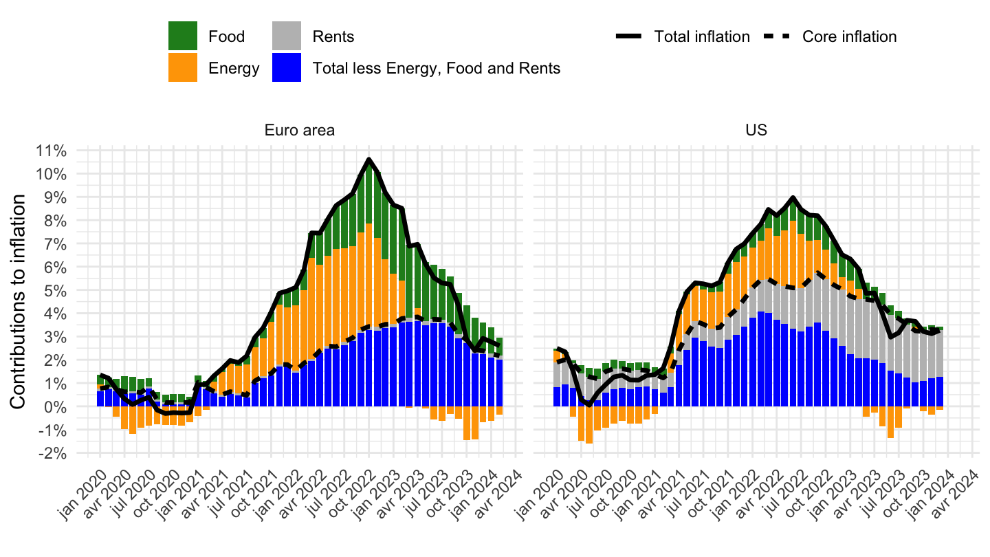
invisible(Sys.setlocale("LC_TIME", "fr_CA.UTF-8"))
# OECD ne publie plus la décomposition de la contribution à l'inflation pour
# l'énergie (CPGREN01) et le sous-jacent (CPGRLE01) aux États-Unis après
# 2023-12, alors que la contribution totale / alimentation / loyers et le taux
# de variation sur un an de l'énergie (GY) vont jusqu'à aujourd'hui. On comble
# la contribution de l'énergie manquante par w * GY, où w est le poids de
# l'énergie dans l'IPC implicite sur la période de recouvrement ; le résidu
# (Total sans énergie, alimentation, loyers) absorbe le faible écart de
# bouclage pour que l'empilement somme toujours à l'inflation totale (CPALTT01).
us_nrg_gy <- PRICES_CPI |>
  filter(MEASURE == "GY", LOCATION == "USA", SUBJECT == "CPGREN01") |>
  month_to_date() |>
  select(date, nrg_gy = obsValue)

us_ctgy <- PRICES_CPI |>
  filter(MEASURE == "CTGY",
         LOCATION %in% c("USA"),
         SUBJECT %in% c("CPGRLE01", "CPGREN01", "CP010000", "CP020000",
                        "CPALTT01", "CP040100", "CP040200")) |>
  month_to_date() |>
  filter(date >= as.Date("2020-01-01")) |>
  select(date, obsValue, SUBJECT) |>
  spread(SUBJECT, obsValue) |>
  left_join(us_nrg_gy, by = "date") |>
  mutate(CPGREN01 = coalesce(CPGREN01,
                             median(CPGREN01 / nrg_gy, na.rm = TRUE) * nrg_gy))

line_US <- us_ctgy |>
  transmute(date, Inflation = CPALTT01,
            `Inflation sous-jacente` = CPALTT01 - (CP010000 + CP020000) - CPGREN01) |>
  gather(Coicop, values, -date) |>
  filter(!is.na(values)) |>
  mutate(Coicop = factor(Coicop, levels = c("Inflation", "Inflation sous-jacente")),
         Geo = "États-Unis")

bars_US <- us_ctgy |>
  transmute(date,
            FOOD = CP010000 + CP020000,
            NRG = CPGREN01,
            RENTS = CP040100+CP040200,
            TOT_X_NRG_FOOD_RENTS = CPALTT01-FOOD-NRG-RENTS) |>
  filter(!is.na(TOT_X_NRG_FOOD_RENTS)) |>
  gather(coicop, values, -date) |>
  # CP070200, CP040500, CP010000
  # CPGRSE01, CPGRGO01
  mutate(Coicop = factor(coicop, levels = c("FOOD", "NRG", "RENTS", "TOT_X_NRG_FOOD_RENTS"),
                         labels = c("Alimentation", "Énergie", "Loyers",
                                    "Total sans énergie, alimentation, loyers")),
         Geo = "États-Unis")

bars_US |>
  ggplot(aes(x = date, y = values/100)) +
  geom_col(aes(fill = Coicop), alpha = 1) +
  geom_line(data = line_US, aes(linetype = Coicop), size = 1.2) +
  theme_minimal() + xlab("") + ylab("Contributions à l'inflation") +
  scale_fill_manual(values = c("forestgreen","orange", "grey", "blue")) +
  scale_x_date(breaks ="3 months",
               labels = date_format("%b %Y")) +
  scale_y_continuous(breaks = 0.01*seq(-10, 30, 1),
                     labels = percent_format(accuracy = 1)) +
  theme(legend.position = "top",
        legend.title = element_blank(),
        axis.text.x = element_text(angle = 45, vjust = 1, hjust = 1)) +
  guides(fill=guide_legend(nrow=2))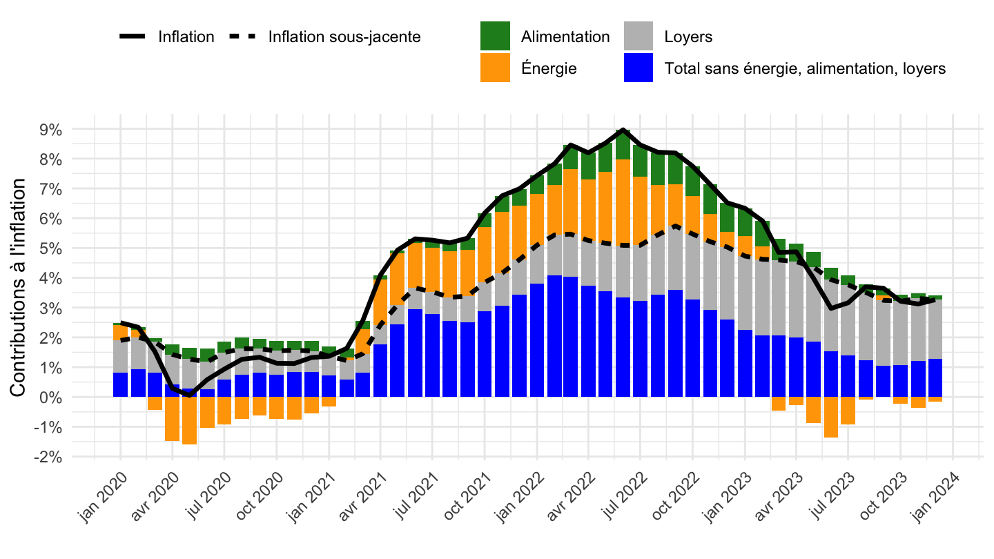
invisible(Sys.setlocale("LC_TIME", "fr_CA.UTF-8"))
load_data("eurostat/prc_hicp_ctrb.RData")
line_EU <- prc_hicp_ctrb |>
  filter(coicop %in% c("NRG", "FOOD", "CP01", "CP02", "CP03", "CP04", "CP05", "CP06",
                       "CP07", "CP08", "CP09", "CP10", "CP11", "CP12", "CP041")) %>%
  mutate(date = gsub("M", "-", time) |> paste0("-01") |> as.Date()) |>
  filter(date >= as.Date("2020-01-01")) |>
  select(date, values, coicop) |>
  spread(coicop, values) |>
  transmute(date,
            `Total inflation` = CP01+CP02+CP03+CP04+CP05+CP06+CP07+CP08+CP09+CP10+CP11+CP12,
            FOOD,
            NRG,
            `Core inflation` = `Total inflation`-FOOD-NRG) |>
  select(date, Inflation = `Total inflation`, `Inflation sous-jacente` = `Core inflation`) |>
  gather(Coicop, values, -date) |>
  mutate(Coicop = factor(Coicop, levels = c("Inflation", "Inflation sous-jacente")),
         Geo = "Zone euro")

bars_EU <- prc_hicp_ctrb |>
  filter(coicop %in% c("NRG", "FOOD", "CP01", "CP02", "CP03", "CP04", "CP05", "CP06",
                       "CP07", "CP08", "CP09", "CP10", "CP11", "CP12", "CP041")) %>%
  mutate(date = gsub("M", "-", time) |> paste0("-01") |> as.Date()) |>
  filter(date >= as.Date("2020-01-01")) |>
  select(date, values, coicop) |>
  spread(coicop, values) |>
  transmute(date,
            FOOD,
            NRG,
            RENTS = CP041,
            `Total inflation` = CP01+CP02+CP03+CP04+CP05+CP06+CP07+CP08+CP09+CP10+CP11+CP12,
            TOT_X_NRG_FOOD_RENTS = `Total inflation`-FOOD-NRG-RENTS) |>
  select(-`Total inflation`) |>
  gather(coicop, values, -date) |>
  # CP070200, CP040500, CP010000
  # CPGRSE01, CPGRGO01
  mutate(Coicop = factor(coicop, levels = c("FOOD", "NRG", "RENTS", "TOT_X_NRG_FOOD_RENTS"),
                         labels = c("Alimentation", "Énergie", "Loyers",
                                    "Total sans énergie, alimentation, loyers")),
         Geo = "Zone euro")

bars_EU |>
  ggplot(aes(x = date, y = values/100)) +
  geom_col(aes(fill = Coicop), alpha = 1) +
  geom_line(data = line_EU, aes(linetype = Coicop), size = 1.2) +
  theme_minimal() + xlab("") + ylab("Contributions à l'inflation") +
  scale_fill_manual(values = c("forestgreen","orange", "grey", "blue")) +
  scale_x_date(breaks ="3 months",
               labels = date_format("%b %Y")) +
  scale_y_continuous(breaks = 0.01*seq(-10, 30, 1),
                     labels = percent_format(accuracy = 1)) +
  theme(legend.position = "top",
        legend.title = element_blank(),
        axis.text.x = element_text(angle = 45, vjust = 1, hjust = 1)) +
  guides(fill=guide_legend(nrow=2))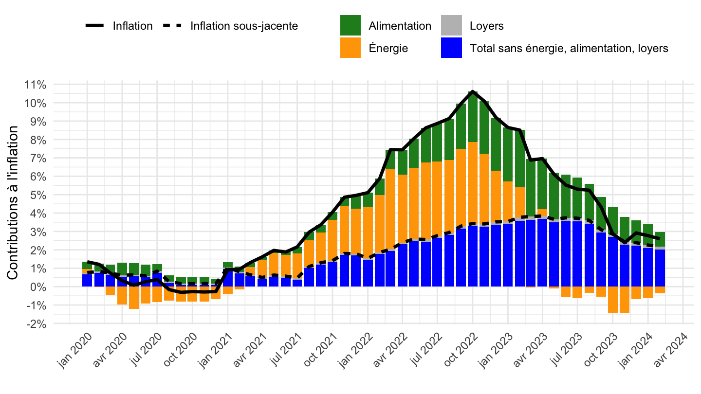
bars_EU |>
  bind_rows(bars_US) |>
  mutate(Geo = factor(Geo, levels = c("Zone euro", "États-Unis"))) |>
  ggplot(aes(x = date, y = values/100)) +
  geom_col(aes(fill = Coicop), alpha = 1) +
  geom_line(data = line_EU |>
              bind_rows(line_US) |>
              mutate(Geo = factor(Geo, levels = c("Zone euro", "États-Unis"))),
            aes(linetype = Coicop), size = 1.2) +
  theme_minimal() + xlab("") + ylab("Contributions à l'inflation") +
  scale_fill_manual(values = c("forestgreen","orange", "grey", "blue")) +
  scale_x_date(breaks ="6 months",
               labels = date_format("%b %Y"),
               expand = expansion(mult = 0.02)) +
  scale_y_continuous(breaks = 0.01*seq(-10, 30, 1),
                     labels = percent_format(accuracy = 1)) +
  theme(legend.position = "top",
        legend.title = element_blank(),
        axis.text.x = element_text(angle = 45, vjust = 1, hjust = 1)) +
  guides(fill=guide_legend(nrow=2)) +
  facet_wrap(~ Geo, scales = "free_x")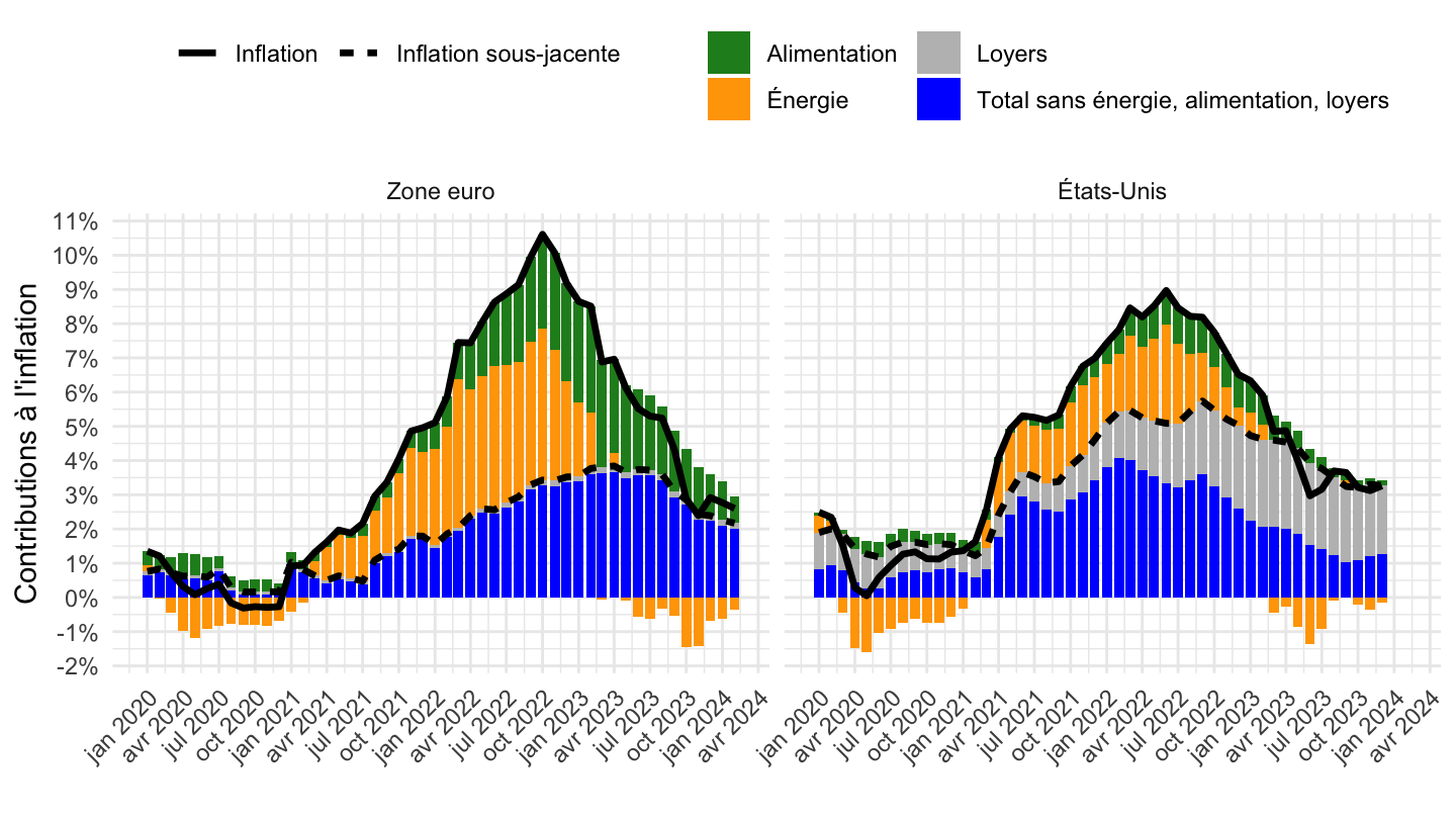
PRICES_CPI |>
  filter(LOCATION %in% c("FRA", "DEU"),
         SUBJECT %in% c("CPHPTT01", "CPALTT01"),
         FREQUENCY == "M",
         MEASURE == "IXOB") |>
  month_to_date() |>
  select(date, SUBJECT, LOCATION, obsValue) |>
  filter(date >= as.Date("1996-01-01")) |>
  left_join(PRICES_CPI_var$LOCATION, by = "LOCATION") |>
  left_join(PRICES_CPI_var$SUBJECT, by = "SUBJECT") |>
  add_flag_color("Location") |>
  mutate(Location2 = ifelse(LOCATION == "DEU", "Allemagne", Location)) |>
  group_by(LOCATION, Subject) |>
  mutate(obsValue = 100*obsValue/obsValue[1]) |>
  ggplot() + geom_line(aes(x = date, y = obsValue, color = Location, linetype = Subject)) +
  scale_color_manual(values = c("#000000", "#ED2939")) +
  scale_linetype_manual(values = c("dashed", "solid")) + add_4flags +
  theme_minimal() + xlab("") + ylab("Price Index") +
  scale_x_date(breaks = seq(1960, 2100, 1) |> paste0("-01-01") |> as.Date(),
               labels = date_format("%Y")) +
  theme(legend.position = c(0.15, 0.8),
        legend.title = element_blank(),
        axis.text.x = element_text(angle = 45, vjust = 1, hjust = 1)) +
  scale_y_log10(breaks = seq(10, 200, 5))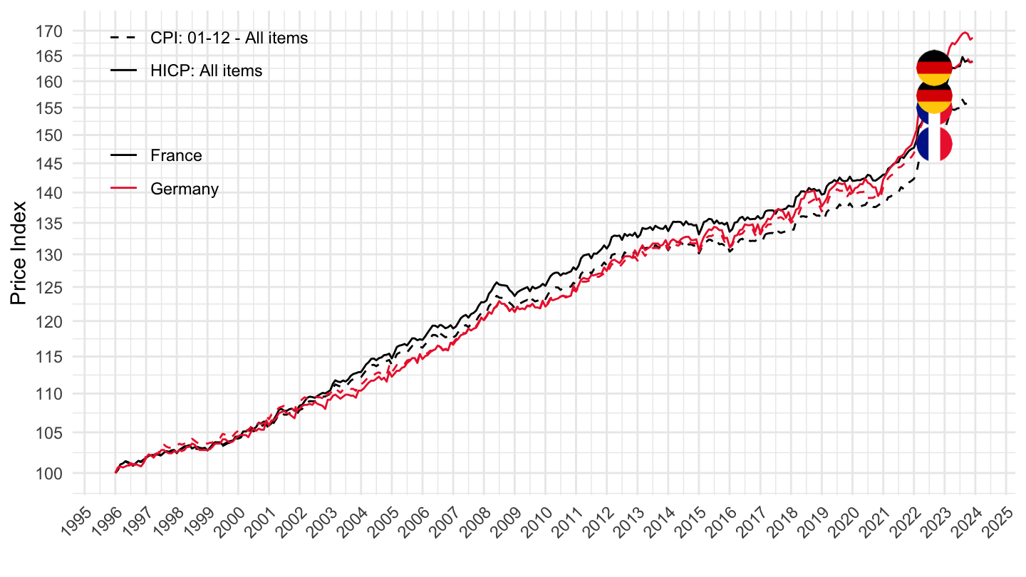
PRICES_CPI |>
  filter(LOCATION %in% c("FRA", "DEU"),
         SUBJECT %in% c("CPHPTT01", "CPALTT01"),
         FREQUENCY == "M",
         MEASURE == "IXOB") |>
  month_to_date() |>
  select(date, SUBJECT, LOCATION, obsValue) |>
  filter(date >= as.Date("1999-01-01")) |>
  left_join(PRICES_CPI_var$LOCATION, by = "LOCATION") |>
  left_join(PRICES_CPI_var$SUBJECT, by = "SUBJECT") |>
  add_flag_color("Location") |>
  mutate(Location2 = ifelse(LOCATION == "DEU", "Allemagne", Location)) |>
  group_by(LOCATION, Subject) |>
  mutate(obsValue = 100*obsValue/obsValue[1]) |>
  ggplot() + geom_line(aes(x = date, y = obsValue, color = Location, linetype = Subject)) +
  scale_color_manual(values = c("#000000", "#ED2939")) +
  scale_linetype_manual(values = c("dashed", "solid")) + add_4flags +
  theme_minimal() + xlab("") + ylab("Price Index") +
  scale_x_date(breaks = seq(1960, 2100, 1) |> paste0("-01-01") |> as.Date(),
               labels = date_format("%Y")) +
  theme(legend.position = c(0.15, 0.8),
        legend.title = element_blank(),
        axis.text.x = element_text(angle = 45, vjust = 1, hjust = 1)) +
  scale_y_log10(breaks = seq(10, 200, 5))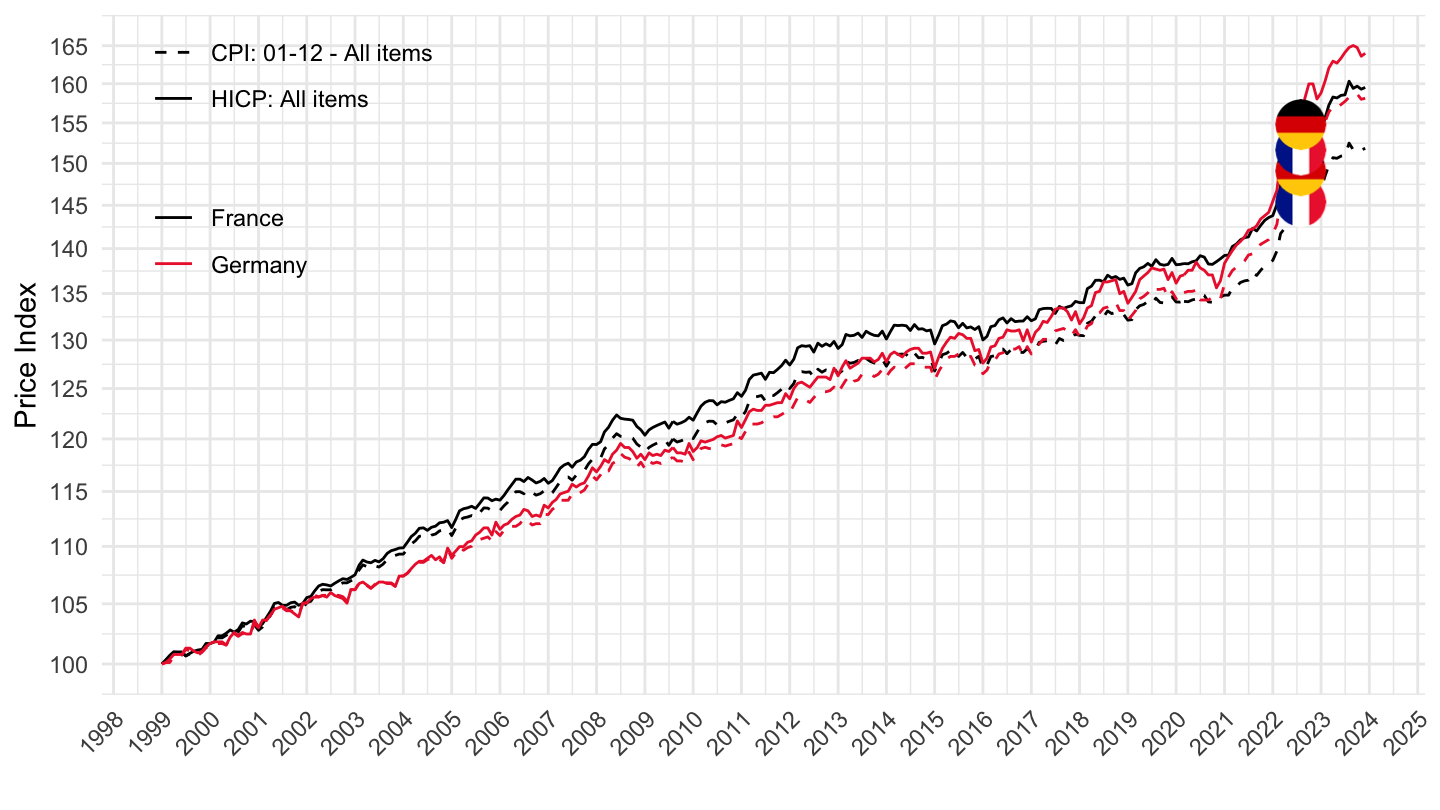
PRICES_CPI |>
  filter(LOCATION %in% c("FRA", "DEU"),
         SUBJECT %in% c("CPHPTT01", "CPALTT01"),
         FREQUENCY == "M",
         MEASURE == "IXOB") |>
  month_to_date() |>
  select(date, SUBJECT, LOCATION, obsValue) |>
  filter(date >= as.Date("2008-01-01")) |>
  left_join(PRICES_CPI_var$LOCATION, by = "LOCATION") |>
  left_join(PRICES_CPI_var$SUBJECT, by = "SUBJECT") |>
  add_flag_color("Location") |>
  mutate(Location2 = ifelse(LOCATION == "DEU", "Allemagne", Location)) |>
  group_by(LOCATION, Subject) |>
  mutate(obsValue = 100*obsValue/obsValue[1]) |>
  ggplot() + geom_line(aes(x = date, y = obsValue, color = Location, linetype = Subject)) +
  scale_color_manual(values = c("#000000", "#ED2939")) +
  scale_linetype_manual(values = c("dashed", "solid")) + add_4flags +
  theme_minimal() + xlab("") + ylab("Price Index") +
  scale_x_date(breaks = seq(1960, 2100, 1) |> paste0("-01-01") |> as.Date(),
               labels = date_format("%Y")) +
  theme(legend.position = c(0.15, 0.8),
        legend.title = element_blank(),
        axis.text.x = element_text(angle = 45, vjust = 1, hjust = 1)) +
  scale_y_log10(breaks = seq(10, 200, 5))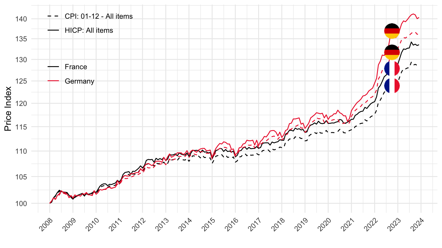
PRICES_CPI |>
  filter(LOCATION %in% c("FRA", "DEU"),
         SUBJECT %in% c("CPHPTT01", "CPALTT01"),
         FREQUENCY == "M",
         MEASURE == "IXOB") |>
  month_to_date() |>
  select(date, SUBJECT, LOCATION, obsValue) |>
  filter(date >= as.Date("2015-01-01")) |>
  left_join(PRICES_CPI_var$LOCATION, by = "LOCATION") |>
  left_join(PRICES_CPI_var$SUBJECT, by = "SUBJECT") |>
  add_flag_color("Location") |>
  group_by(LOCATION, Subject) |>
  mutate(obsValue = 100*obsValue/obsValue[1]) |>
  mutate(Location2 = ifelse(LOCATION == "DEU", "Allemagne", Location)) |>
  ggplot() + geom_line(aes(x = date, y = obsValue, color = Location, linetype = Subject)) +
  scale_color_manual(values = c("#000000", "#ED2939")) +
  scale_linetype_manual(values = c("dashed", "solid")) + add_4flags +
  theme_minimal() + xlab("") + ylab("Price Index") +
  scale_x_date(breaks = seq(1960, 2100, 1) |> paste0("-01-01") |> as.Date(),
               labels = date_format("%Y")) +
  theme(legend.position = c(0.15, 0.8),
        legend.title = element_blank(),
        axis.text.x = element_text(angle = 45, vjust = 1, hjust = 1)) +
  scale_y_log10(breaks = seq(10, 200, 5))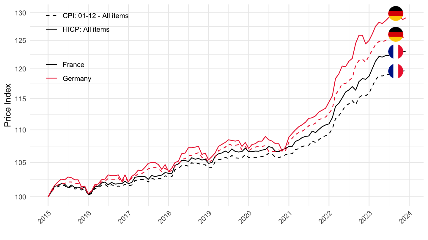
PRICES_CPI |>
  filter(LOCATION %in% c("FRA", "DEU"),
         SUBJECT %in% c("CPHPTT01", "CPALTT01"),
         FREQUENCY == "M",
         MEASURE == "IXOB") |>
  month_to_date() |>
  select(date, SUBJECT, LOCATION, obsValue) |>
  filter(date >= as.Date("2017-01-01")) |>
  left_join(PRICES_CPI_var$LOCATION, by = "LOCATION") |>
  left_join(PRICES_CPI_var$SUBJECT, by = "SUBJECT") |>
  add_flag_color("Location") |>
  group_by(LOCATION, Subject) |>
  mutate(obsValue = 100*obsValue/obsValue[1]) |>
  mutate(Location2 = ifelse(LOCATION == "DEU", "Allemagne", Location)) |>
  ggplot() + geom_line(aes(x = date, y = obsValue, color = Location, linetype = Subject)) +
  scale_color_manual(values = c("#000000", "#ED2939")) +
  scale_linetype_manual(values = c("dashed", "solid")) + add_4flags +
  theme_minimal() + xlab("") + ylab("Price Index") +
  scale_x_date(breaks = seq(1960, 2100, 1) |> paste0("-01-01") |> as.Date(),
               labels = date_format("%Y")) +
  theme(legend.position = c(0.15, 0.8),
        legend.title = element_blank(),
        axis.text.x = element_text(angle = 45, vjust = 1, hjust = 1)) +
  scale_y_log10(breaks = seq(10, 200, 5))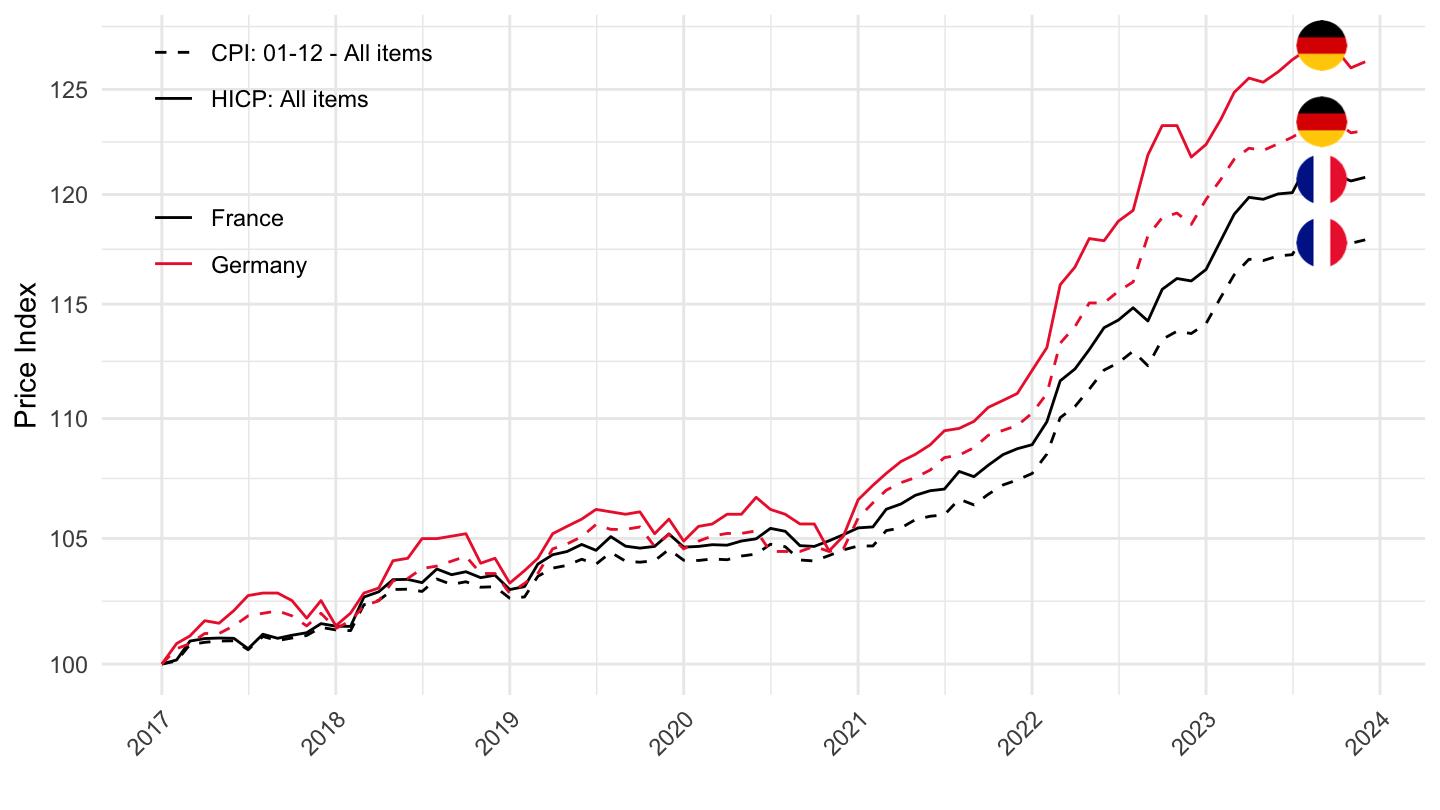
PRICES_CPI |>
  filter(SUBJECT == "CPALTT01",
         MEASURE == "GP") |>
  group_by(LOCATION, FREQUENCY) |>
  summarise(Nobs = n()) |>
  left_join(PRICES_CPI_var$LOCATION, by = "LOCATION") |>
  spread(FREQUENCY, Nobs) |>
  arrange(-M) |>
  mutate(Flag = gsub(" ", "-", str_to_lower(Location)),
         Flag = paste0('<img src="../../icon/flag/vsmall/', Flag, '.png" alt="Flag">')) |>
  select(Flag, everything()) %>%
{if (is_html_output()) datatable(., filter = 'top', rownames = F, escape = F) else .}PRICES_CPI |>
filter(SUBJECT == "CPHPTT01",
MEASURE == "GY") |>
group_by(LOCATION, FREQUENCY) |>
summarise(Nobs = n()) |>
left_join(PRICES_CPI_var$LOCATION, by = "LOCATION") |>
spread(FREQUENCY, Nobs) |>
arrange(-M) |>
mutate(Flag = gsub(" ", "-", str_to_lower(Location)),
Flag = paste0('<img src="../../icon/flag/vsmall/', Flag, '.png" alt="Flag">')) |>
select(Flag, everything()) %>%
{if (is_html_output()) datatable(., filter = 'top', rownames = F, escape = F) else .}PRICES_CPI |>
filter(SUBJECT == "CPALTT01",
MEASURE == "GP") |>
filter(obsValue >= 10) |>
arrange(-obsValue) |>
left_join(PRICES_CPI_var$LOCATION, by = "LOCATION") |>
select(obsTime, Location, FREQUENCY, obsValue) |>
print_table_conditional()PRICES_CPI |>
filter(LOCATION %in% c("KOR"),
SUBJECT %in% c("CPALTT01"),
FREQUENCY == "A",
MEASURE == "GP") |>
year_to_date() |>
select(date, LOCATION, obsValue) |>
mutate(obsValue = obsValue / 100) |>
left_join(PRICES_CPI_var$LOCATION, by = "LOCATION") |>
add_flag_color("Location") |>
ggplot() + geom_line(aes(x = date, y = obsValue)) +
scale_color_identity() +
theme_minimal() + xlab("") + ylab("Inflation (%)") +
scale_x_date(breaks = seq(1960, 2100, 5) |> paste0("-01-01") |> as.Date(),
labels = date_format("%Y")) +
scale_y_continuous(breaks = 0.01*seq(-100, 200, 2),
labels = percent_format(acc = 1))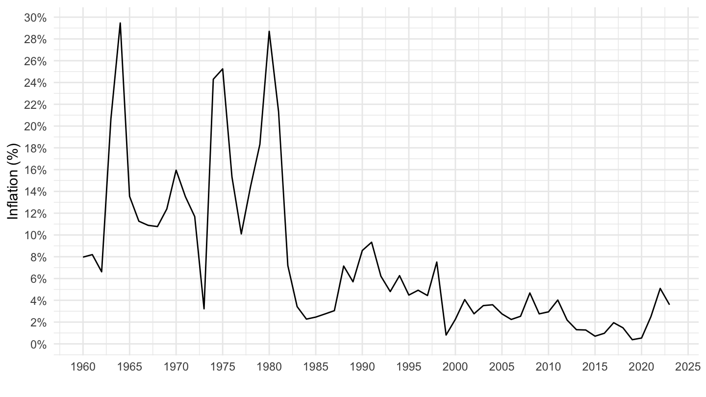
PRICES_CPI |>
  filter(LOCATION %in% c("POL", "HUN"),
         SUBJECT %in% c("CPALTT01"),
         FREQUENCY == "A",
         MEASURE == "GP") |>
  year_to_date() |>
  select(date, LOCATION, obsValue) |>
  mutate(obsValue = obsValue / 100) |>
  left_join(PRICES_CPI_var$LOCATION, by = "LOCATION") |>
  add_flag_color("Location") |>
  ggplot() + geom_line(aes(x = date, y = obsValue, color = color)) +
  scale_color_identity() + add_2flags +
  theme_minimal() + xlab("") + ylab("Inflation (%)") +
  scale_x_date(breaks = seq(1960, 2100, 5) |> paste0("-01-01") |> as.Date(),
               labels = date_format("%Y")) +
  scale_y_continuous(breaks = 0.01*seq(-100, 200, 2),
                     labels = percent_format(acc = 1))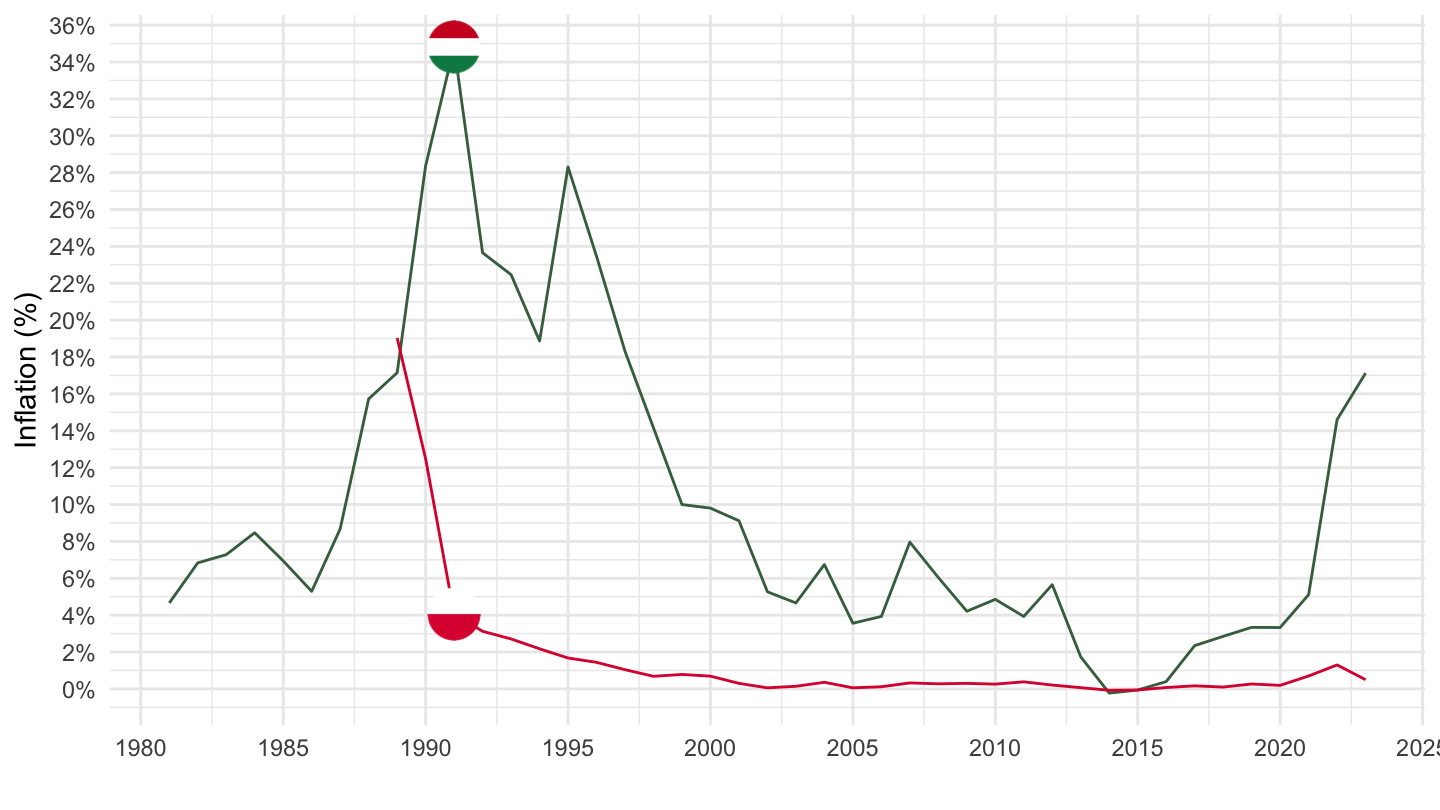
PRICES_CPI |>
  filter(LOCATION %in% c("POL", "HUN"),
         SUBJECT %in% c("CPALTT01"),
         FREQUENCY == "Q",
         MEASURE == "GY") |>
  quarter_to_date() |>
  select(date, LOCATION, obsValue) |>
  mutate(obsValue = obsValue / 100) |>
  left_join(PRICES_CPI_var$LOCATION, by = "LOCATION") |>
  add_flag_color("Location") |>
  ggplot() + geom_line(aes(x = date, y = obsValue, color = color)) +
  scale_color_identity() + add_2flags +
  theme_minimal() + xlab("") + ylab("Inflation (%)") +
  scale_x_date(breaks = seq(1960, 2100, 5) |> paste0("-01-01") |> as.Date(),
               labels = date_format("%Y")) +
  scale_y_continuous(breaks = 0.01*seq(-100, 200, 1),
                     labels = percent_format(acc = 1))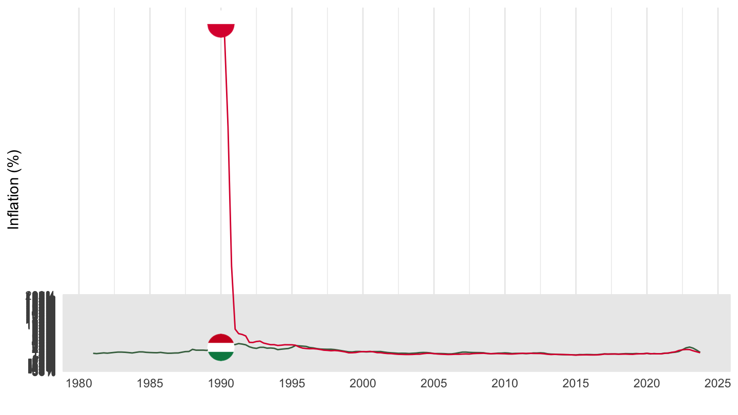
PRICES_CPI |>
  filter(LOCATION %in% c("FRA", "ITA", "DEU", "CAN"),
         SUBJECT %in% c("CPALTT01"),
         FREQUENCY == "A",
         MEASURE == "GP") |>
  year_to_date() |>
  select(date, LOCATION, obsValue) |>
  mutate(obsValue = obsValue / 100) |>
  left_join(PRICES_CPI_var$LOCATION, by = "LOCATION") |>
  add_flag_color("Location") |>
  ggplot() + geom_line(aes(x = date, y = obsValue, color = color)) +
  scale_color_identity() + add_4flags +
  theme_minimal() + xlab("") + ylab("Inflation (%)") +
  scale_x_date(breaks = seq(1960, 2100, 5) |> paste0("-01-01") |> as.Date(),
               labels = date_format("%Y")) +
  scale_y_continuous(breaks = 0.01*seq(-100, 200, 2),
                     labels = percent_format(acc = 1))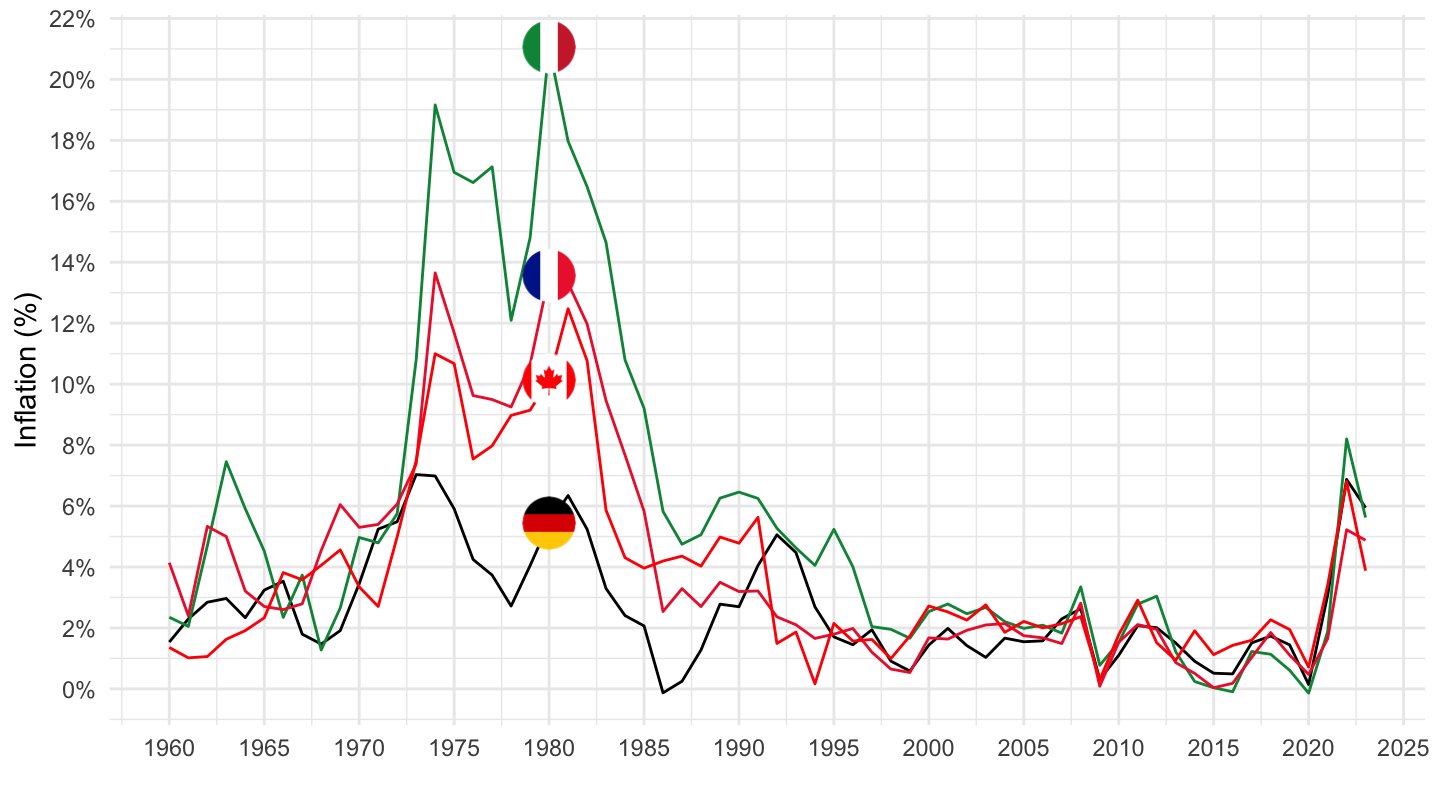
PRICES_CPI |>
  filter(LOCATION %in% c("FRA", "ITA", "DEU", "CAN"),
         SUBJECT %in% c("CPALTT01"),
         FREQUENCY == "Q",
         MEASURE == "GY") |>
  quarter_to_date() |>
  select(date, LOCATION, obsValue) |>
  mutate(obsValue = obsValue / 100) |>
  left_join(PRICES_CPI_var$LOCATION, by = "LOCATION") |>
  add_flag_color("Location") |>
  ggplot() + geom_line(aes(x = date, y = obsValue, color = color)) +
  scale_color_identity() + add_4flags +
  theme_minimal() + xlab("") + ylab("Inflation (%)") +
  scale_x_date(breaks = seq(1960, 2100, 5) |> paste0("-01-01") |> as.Date(),
               labels = date_format("%Y")) +
  scale_y_continuous(breaks = 0.01*seq(-100, 200, 1),
                     labels = percent_format(acc = 1))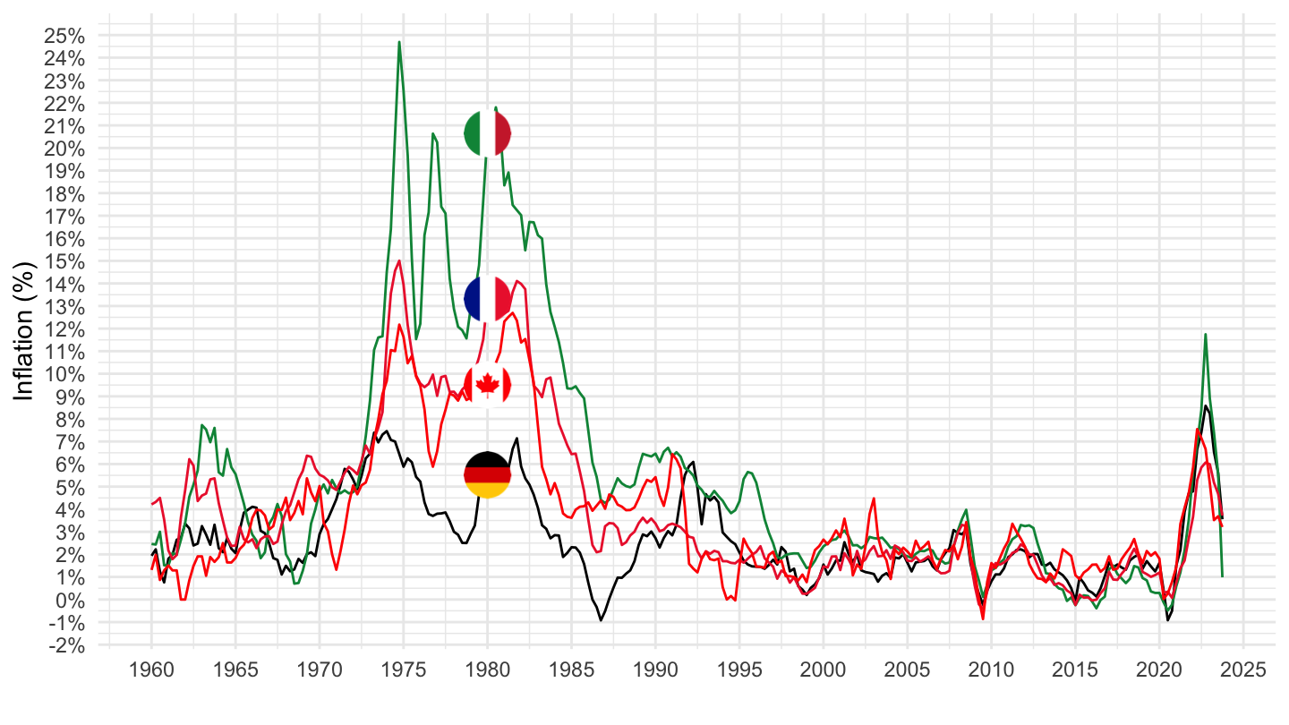
PRICES_CPI |>
  filter(LOCATION %in% c("FRA", "DEU"),
         SUBJECT %in% c("CPALTT01"),
         FREQUENCY == "M",
         MEASURE == "GY") |>
  month_to_date() |>
  select(date, LOCATION, obsValue) |>
  mutate(obsValue = obsValue / 100) |>
  left_join(PRICES_CPI_var$LOCATION, by = "LOCATION") |>
  add_flag_color("Location") |>
  mutate(Location2 = ifelse(LOCATION == "DEU", "Allemagne", Location)) |>
  ggplot() + geom_line(aes(x = date, y = obsValue, color = Location2, linetype = Location2)) +
  scale_color_manual(values = c("#000000", "#ED2939")) +
  scale_linetype_manual(values = c("dashed", "solid")) +
  add_2flags +
  theme_minimal() + xlab("") + ylab("Inflation, Glissement sur un an (%)") +
  scale_x_date(breaks = seq(1960, 2100, 5) |> paste0("-01-01") |> as.Date(),
               labels = date_format("%Y")) +
  theme(legend.position = c(0.7, 0.9),
        legend.title = element_blank()) +
  scale_y_continuous(breaks = 0.01*seq(-100, 200, 1),
                     labels = percent_format(acc = 1))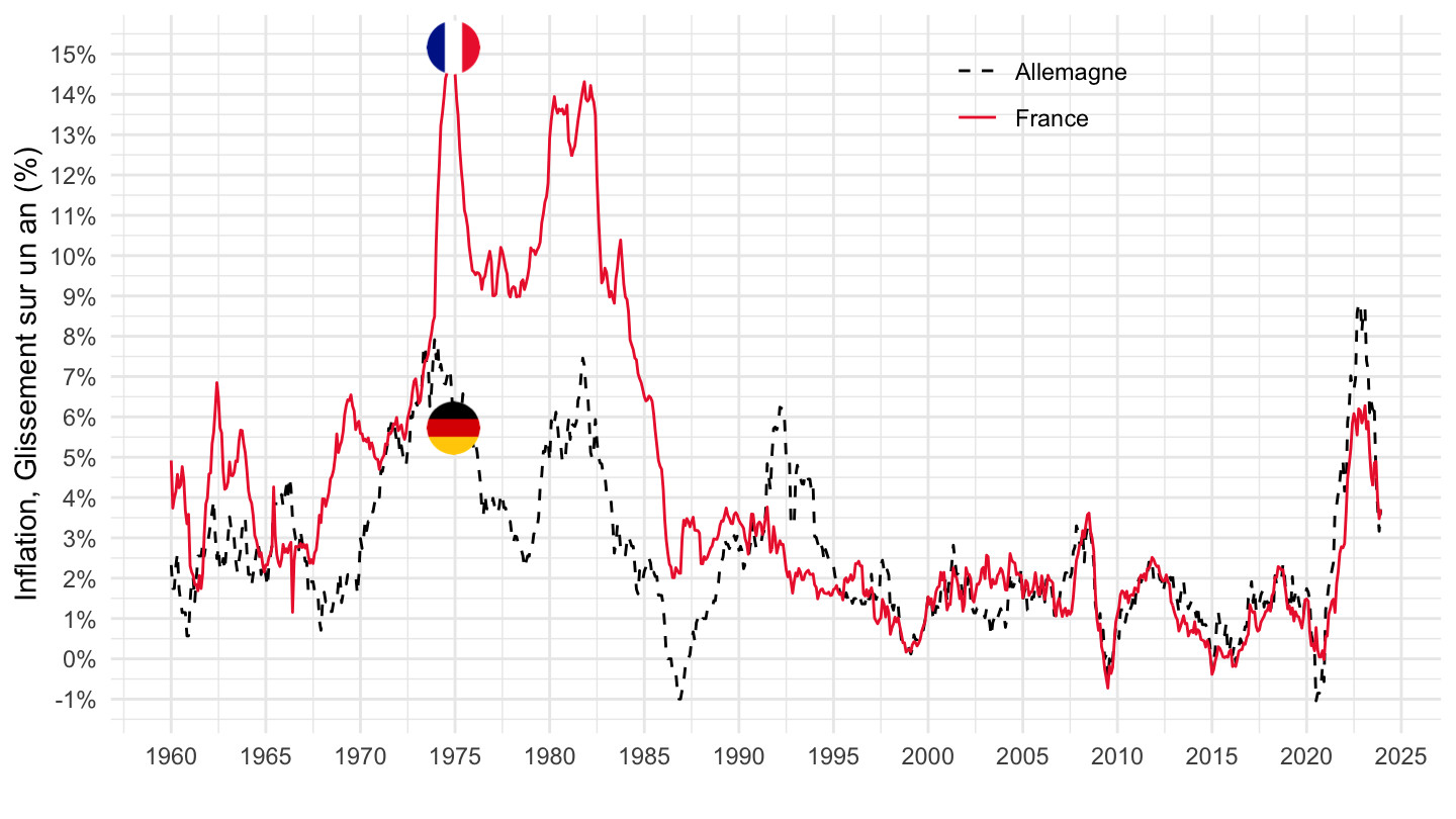
PRICES_CPI |>
  filter(LOCATION %in% c("FRA", "DEU"),
         SUBJECT %in% c("CPALTT01"),
         FREQUENCY == "M",
         MEASURE == "GY") |>
  month_to_date() |>
  select(date, LOCATION, obsValue) |>
  mutate(obsValue = obsValue / 100) |>
  filter(date >= as.Date("2015-01-01")) |>
  left_join(PRICES_CPI_var$LOCATION, by = "LOCATION") |>
  add_flag_color("Location") |>
  mutate(Location2 = ifelse(LOCATION == "DEU", "Allemagne", Location)) |>
  ggplot() + geom_line(aes(x = date, y = obsValue, color = Location2)) +
  scale_color_manual(values = c("#000000", "#ED2939")) +
  scale_linetype_manual(values = c("dashed", "solid")) +
  add_2flags +
  theme_minimal() + xlab("") + ylab("Inflation, Glissement sur un an (%)") +
  scale_x_date(breaks = seq(1960, 2100, 1) |> paste0("-01-01") |> as.Date(),
               labels = date_format("%Y")) +
  theme(legend.position = c(0.2, 0.9),
        legend.title = element_blank()) +
  scale_y_continuous(breaks = 0.01*seq(-100, 200, 1),
                     labels = percent_format(acc = 1))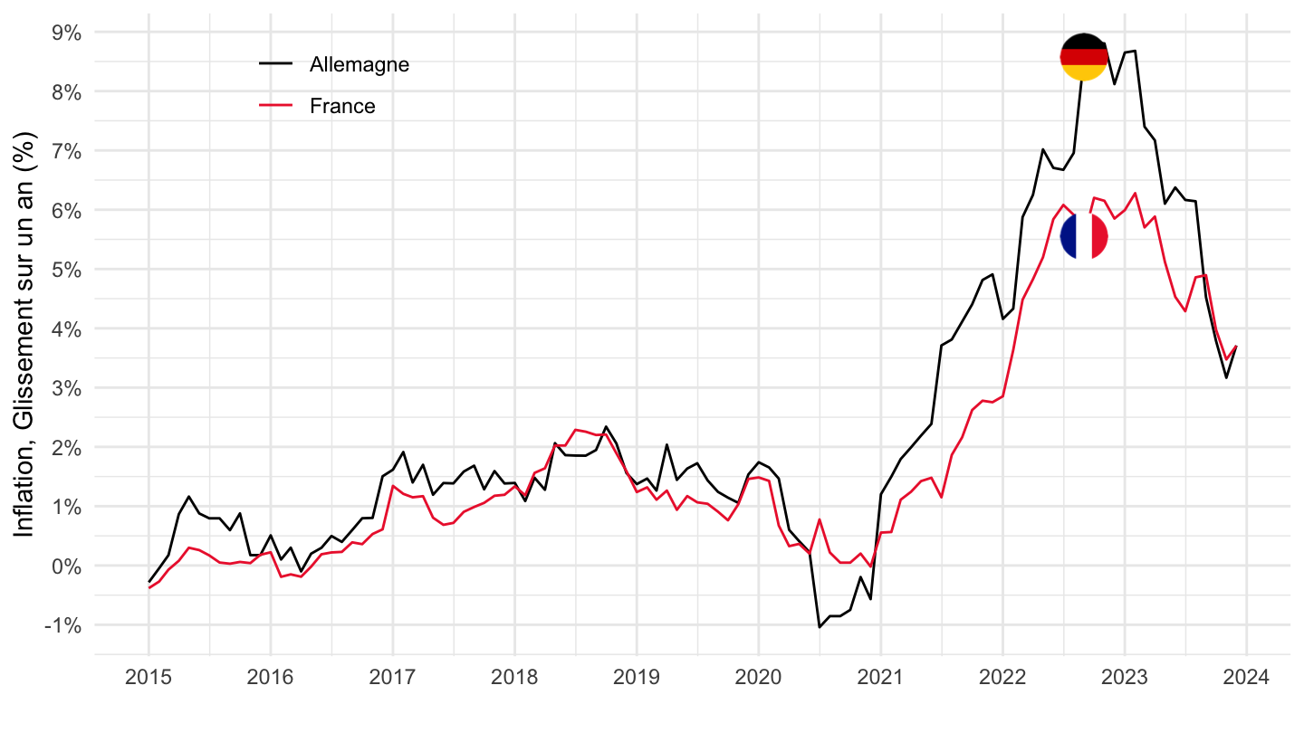
PRICES_CPI |>
  filter(LOCATION %in% c("FRA", "DEU"),
         SUBJECT %in% c("CPHPTT01", "CPALTT01"),
         FREQUENCY == "M",
         MEASURE == "GY") |>
  month_to_date() |>
  select(date, SUBJECT, LOCATION, obsValue) |>
  mutate(obsValue = obsValue / 100) |>
  filter(date >= as.Date("2015-01-01")) |>
  left_join(PRICES_CPI_var$LOCATION, by = "LOCATION") |>
  left_join(PRICES_CPI_var$SUBJECT, by = "SUBJECT") |>
  add_flag_color("Location") |>
  mutate(Location2 = ifelse(LOCATION == "DEU", "Allemagne", Location)) |>
  ggplot() + geom_line(aes(x = date, y = obsValue, color = Location, linetype = Subject)) +
  scale_color_manual(values = c("#000000", "#ED2939")) +
  scale_linetype_manual(values = c("dashed", "solid")) + add_4flags +
  theme_minimal() + xlab("") + ylab("1 year inflation (%)") +
  scale_x_date(breaks = seq(1960, 2100, 1) |> paste0("-01-01") |> as.Date(),
               labels = date_format("%Y")) +
  theme(legend.position = c(0.15, 0.8),
        legend.title = element_blank(),
        axis.text.x = element_text(angle = 45, vjust = 1, hjust = 1)) +
  scale_y_continuous(breaks = 0.01*seq(-100, 200, 1),
                     labels = percent_format(acc = 1))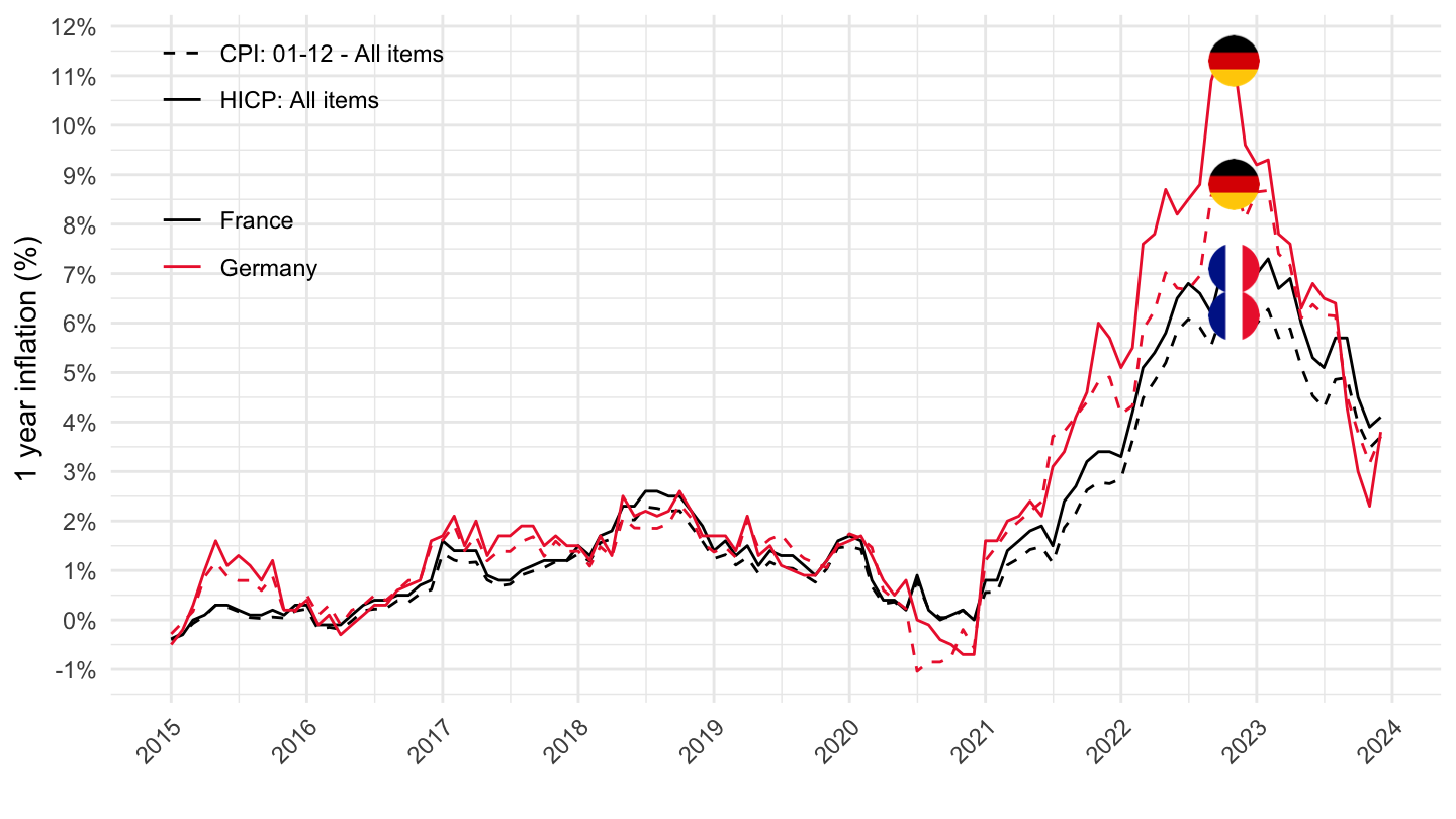
PRICES_CPI |>
  filter(LOCATION %in% c("FRA", "DEU"),
         SUBJECT %in% c("CPALTT01"),
         FREQUENCY == "M",
         MEASURE == "GY") |>
  month_to_date() |>
  select(date, LOCATION, obsValue) |>
  mutate(obsValue = obsValue / 100) |>
  filter(date >= as.Date("2020-01-01")) |>
  left_join(PRICES_CPI_var$LOCATION, by = "LOCATION") |>
  add_flag_color("Location") |>
  mutate(Location2 = ifelse(LOCATION == "DEU", "Allemagne", Location)) |>
  ggplot() + geom_line(aes(x = date, y = obsValue, color = Location2)) +
  scale_color_manual(values = c("#000000", "#ED2939")) +
  scale_linetype_manual(values = c("dashed", "solid")) +
  add_2flags +
  theme_minimal() + xlab("") + ylab("Inflation, Glissement sur un an (%)") +
  scale_x_date(breaks = "2 months",
               labels = date_format("%b %Y")) +
  theme(legend.position = c(0.2, 0.9),
        legend.title = element_blank(),
        axis.text.x = element_text(angle = 45, vjust = 1, hjust = 1)) +
  scale_y_continuous(breaks = 0.01*seq(-100, 200, 1),
                     labels = percent_format(acc = 1)) +
  geom_text_repel(aes(x = date, y = obsValue, label = percent(obsValue, acc = 0.1)),
                  fontface ="plain", color = "black", size = 3)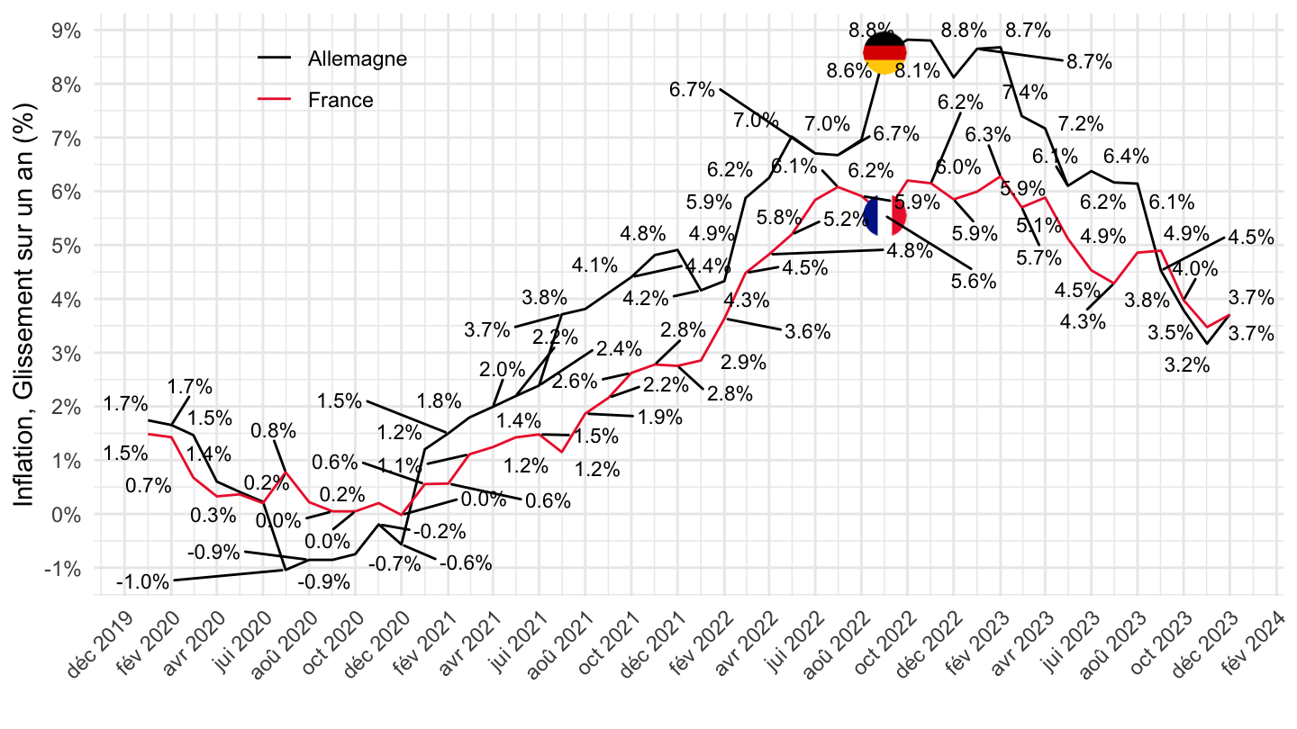
PRICES_CPI |>
  filter(LOCATION %in% c("FRA", "DEU"),
         SUBJECT %in% c("CPHPTT01", "CPALTT01"),
         FREQUENCY == "M",
         MEASURE == "GY") |>
  month_to_date() |>
  select(date, SUBJECT, LOCATION, obsValue) |>
  mutate(obsValue = obsValue / 100) |>
  filter(date >= as.Date("2020-01-01")) |>
  left_join(PRICES_CPI_var$LOCATION, by = "LOCATION") |>
  left_join(PRICES_CPI_var$SUBJECT, by = "SUBJECT") |>
  add_flag_color("Location") |>
  mutate(Location2 = ifelse(LOCATION == "DEU", "Allemagne", Location)) |>
  ggplot() + geom_line(aes(x = date, y = obsValue, color = Location, size = Subject)) +
  scale_color_manual(values = c("#000000", "#ED2939")) +
  scale_size_manual(values = c(0.5, 1)) + add_4flags +
  theme_minimal() + xlab("") + ylab("1 year inflation (%)") +
  scale_x_date(breaks = "2 months",
               labels = date_format("%b %Y")) +
  theme(legend.position = c(0.15, 0.8),
        legend.title = element_blank(),
        axis.text.x = element_text(angle = 45, vjust = 1, hjust = 1)) +
  scale_y_continuous(breaks = 0.01*seq(-100, 200, 1),
                     labels = percent_format(acc = 1)) +
  geom_text_repel(data = . %>%
                        filter(month(date) %in% c(1, 6)), aes(x = date, y = obsValue, label = percent(obsValue, acc = 0.1)),
                  fontface ="plain", color = "black", size = 3)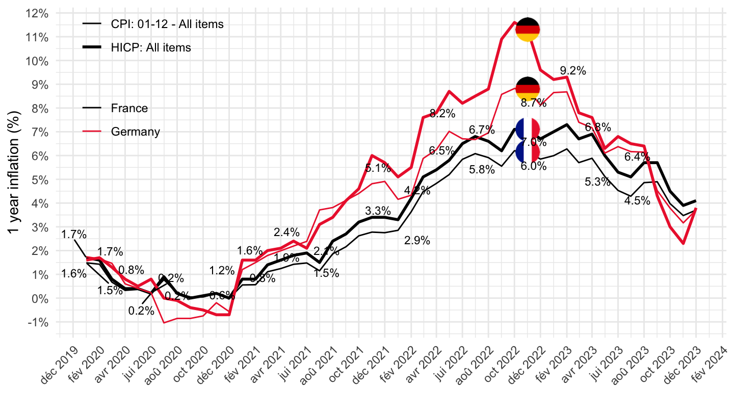
PRICES_CPI |>
  filter(LOCATION %in% c("FRA", "DEU"),
         SUBJECT %in% c("CPALTT01"),
         FREQUENCY == "M",
         MEASURE == "GY") |>
  month_to_date() |>
  select(date, LOCATION, obsValue) |>
  mutate(obsValue = obsValue / 100) |>
  filter(date >= Sys.Date() -years(2)) |>
  left_join(PRICES_CPI_var$LOCATION, by = "LOCATION") |>
  add_flag_color("Location") |>
  mutate(Location2 = ifelse(LOCATION == "DEU", "Allemagne", Location)) |>
  ggplot() + geom_line(aes(x = date, y = obsValue, color = Location)) +
  scale_color_manual(values = c("#000000", "#ED2939")) +
  scale_linetype_manual(values = c("dashed", "solid")) + add_2flags +
  theme_minimal() + xlab("") + ylab("1 year inflation (%)") +
  scale_x_date(breaks = "2 months",
               labels = date_format("%b %Y")) +
  theme(legend.position = c(0.15, 0.9),
        legend.title = element_blank(),
        axis.text.x = element_text(angle = 45, vjust = 1, hjust = 1)) +
  scale_y_continuous(breaks = 0.01*seq(-100, 200, 1),
                     labels = percent_format(acc = 1)) +
  geom_text_repel(aes(x = date, y = obsValue, label = percent(obsValue, acc = 0.1)),
                  fontface ="plain", color = "black", size = 3)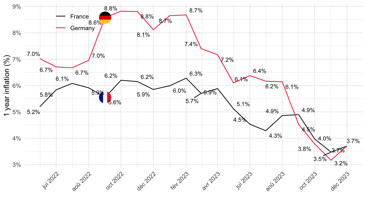
PRICES_CPI |>
  filter(LOCATION %in% c("FRA", "DEU"),
         SUBJECT %in% c("CPHPTT01"),
         FREQUENCY == "M",
         MEASURE == "GY") |>
  month_to_date() |>
  select(date, LOCATION, obsValue) |>
  mutate(obsValue = obsValue / 100) |>
  filter(date >= Sys.Date() -years(2)) |>
  left_join(PRICES_CPI_var$LOCATION, by = "LOCATION") |>
  add_flag_color("Location") |>
  mutate(Location2 = ifelse(LOCATION == "DEU", "Allemagne", Location)) |>
  ggplot() + geom_line(aes(x = date, y = obsValue, color = Location)) +
  scale_color_manual(values = c("#000000", "#ED2939")) +
  scale_linetype_manual(values = c("dashed", "solid")) + add_2flags +
  theme_minimal() + xlab("") + ylab("1 year inflation (%)") +
  scale_x_date(breaks = "2 months",
               labels = date_format("%b %Y")) +
  theme(legend.position = c(0.15, 0.9),
        legend.title = element_blank(),
        axis.text.x = element_text(angle = 45, vjust = 1, hjust = 1)) +
  scale_y_continuous(breaks = 0.01*seq(-100, 200, 1),
                     labels = percent_format(acc = 1)) +
  geom_text_repel(aes(x = date, y = obsValue, label = percent(obsValue, acc = 0.1)),
                  fontface ="plain", color = "black", size = 3)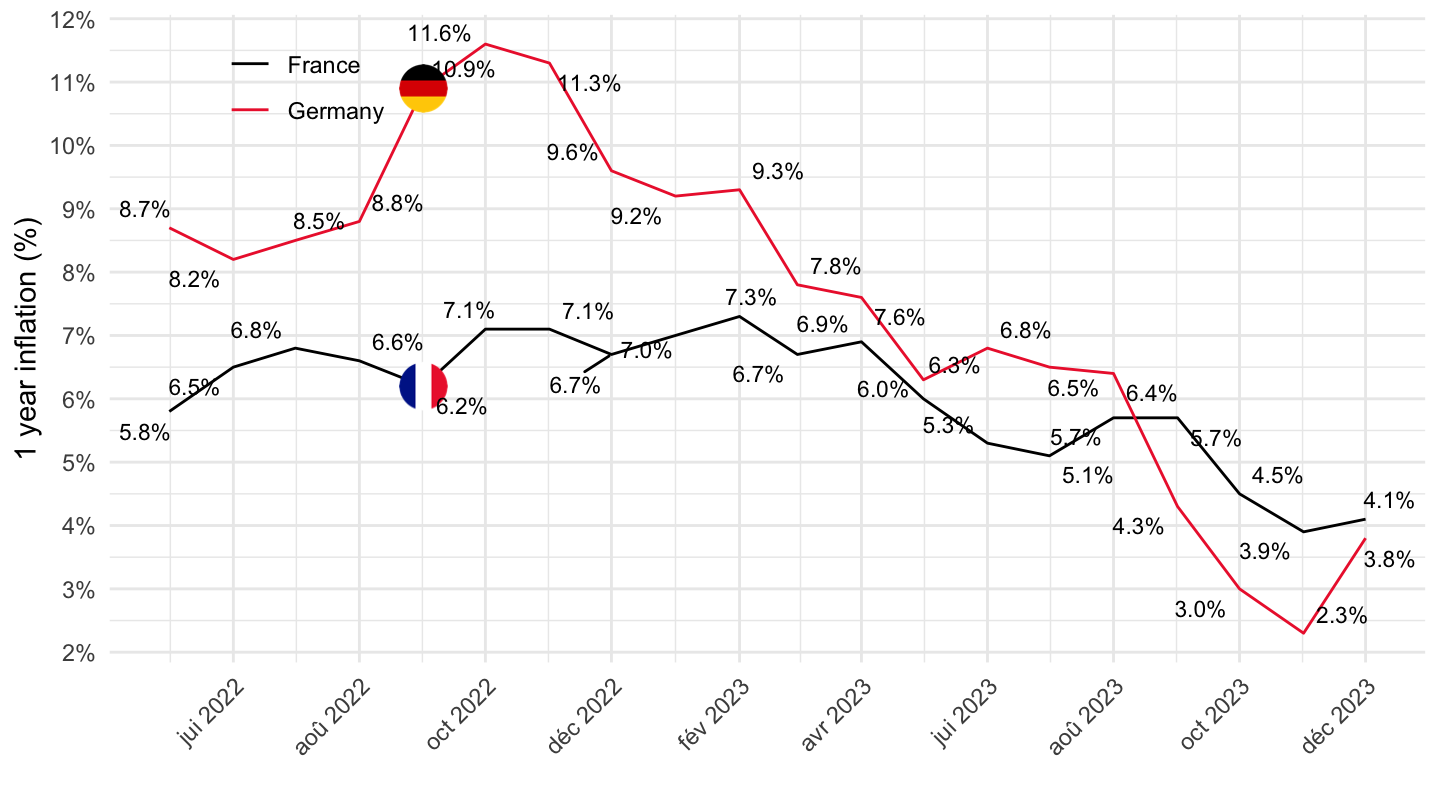
PRICES_CPI |>
  filter(LOCATION %in% c("FRA", "DEU"),
         SUBJECT %in% c("CPHPTT01", "CPALTT01"),
         FREQUENCY == "M",
         MEASURE == "GY") |>
  month_to_date() |>
  select(date, SUBJECT, LOCATION, obsValue) |>
  mutate(obsValue = obsValue / 100) |>
  filter(date >= Sys.Date() -years(2)) |>
  left_join(PRICES_CPI_var$LOCATION, by = "LOCATION") |>
  left_join(PRICES_CPI_var$SUBJECT, by = "SUBJECT") |>
  add_flag_color("Location") |>
  mutate(Location2 = ifelse(LOCATION == "DEU", "Allemagne", Location)) |>
  ggplot() + geom_line(aes(x = date, y = obsValue, color = Location, linetype = Subject)) +
  scale_color_manual(values = c("#000000", "#ED2939")) +
  scale_linetype_manual(values = c("dashed", "solid")) + add_4flags +
  theme_minimal() + xlab("") + ylab("1 year inflation (%)") +
  scale_x_date(breaks = "2 months",
               labels = date_format("%b %Y")) +
  theme(legend.position = c(0.15, 0.8),
        legend.title = element_blank(),
        axis.text.x = element_text(angle = 45, vjust = 1, hjust = 1)) +
  scale_y_continuous(breaks = 0.01*seq(-100, 200, 1),
                     labels = percent_format(acc = 1)) +
  geom_text_repel(aes(x = date, y = obsValue, label = percent(obsValue, acc = 0.1)),
                  fontface ="plain", color = "black", size = 3)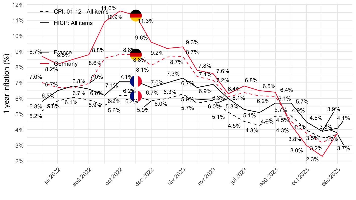
PRICES_CPI |>
  filter(LOCATION %in% c("FRA", "DEU"),
         SUBJECT %in% c("CPALTT01"),
         FREQUENCY == "M",
         MEASURE == "GY") |>
  month_to_date() |>
  select(date, LOCATION, obsValue) |>
  mutate(obsValue = obsValue / 100) |>
  filter(date >= Sys.Date() -years(1)) |>
  left_join(PRICES_CPI_var$LOCATION, by = "LOCATION") |>
  add_flag_color("Location") |>
  mutate(Location2 = ifelse(LOCATION == "DEU", "Allemagne", Location)) |>
  ggplot() + geom_line(aes(x = date, y = obsValue, color = Location)) +
  scale_color_manual(values = c("#000000", "#ED2939")) +
  scale_linetype_manual(values = c("dashed", "solid")) + add_2flags +
  theme_minimal() + xlab("") + ylab("1 year inflation (%)") +
  scale_x_date(breaks = "1 month",
               labels = date_format("%b %Y")) +
  theme(legend.position = c(0.8, 0.9),
        legend.title = element_blank(),
        axis.text.x = element_text(angle = 45, vjust = 1, hjust = 1)) +
  scale_y_continuous(breaks = 0.01*seq(-100, 200, 1),
                     labels = percent_format(acc = 1)) +
  geom_text_repel(aes(x = date, y = obsValue, label = percent(obsValue, acc = 0.1)),
                  fontface ="plain", color = "black", size = 3)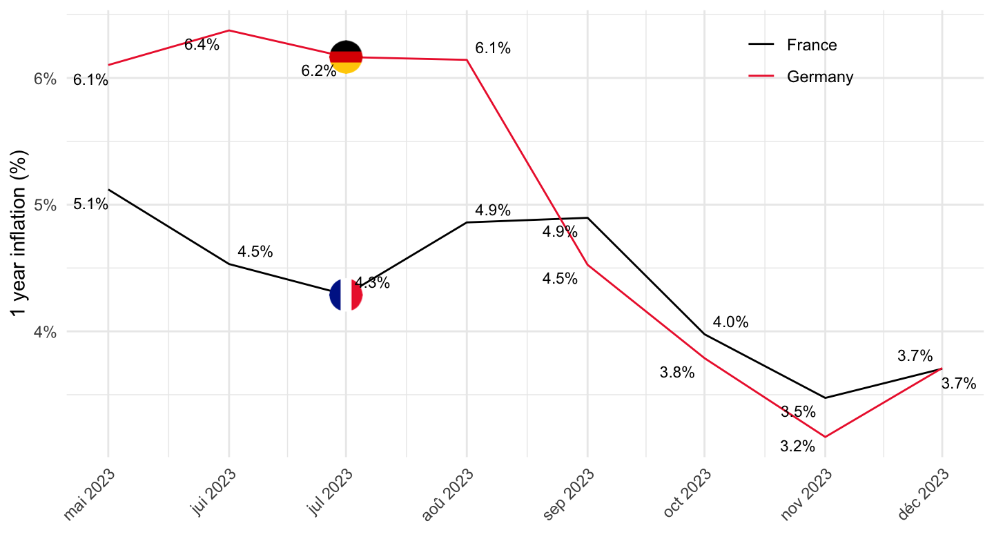
PRICES_CPI |>
  filter(LOCATION %in% c("FRA", "DEU"),
         SUBJECT %in% c("CPHPTT01", "CPALTT01"),
         FREQUENCY == "M",
         MEASURE == "GY") |>
  month_to_date() |>
  select(date, SUBJECT, LOCATION, obsValue) |>
  mutate(obsValue = obsValue / 100) |>
  filter(date >= Sys.Date() -years(1)) |>
  left_join(PRICES_CPI_var$LOCATION, by = "LOCATION") |>
  left_join(PRICES_CPI_var$SUBJECT, by = "SUBJECT") |>
  add_flag_color("Location") |>
  mutate(Location2 = ifelse(LOCATION == "DEU", "Allemagne", Location)) |>
  ggplot() + geom_line(aes(x = date, y = obsValue, color = Location, linetype = Subject)) +
  scale_color_manual(values = c("#000000", "#ED2939")) +
  scale_linetype_manual(values = c("dashed", "solid")) + add_4flags +
  theme_minimal() + xlab("") + ylab("1 year inflation (%)") +
  scale_x_date(breaks = "1 month",
               labels = date_format("%b %Y")) +
  theme(legend.position = c(0.8, 0.7),
        legend.title = element_blank(),
        axis.text.x = element_text(angle = 45, vjust = 1, hjust = 1)) +
  scale_y_continuous(breaks = 0.01*seq(-100, 200, 1),
                     labels = percent_format(acc = 1)) +
  geom_text_repel(aes(x = date, y = obsValue, label = percent(obsValue, acc = 0.1)),
                  fontface ="plain", color = "black", size = 3)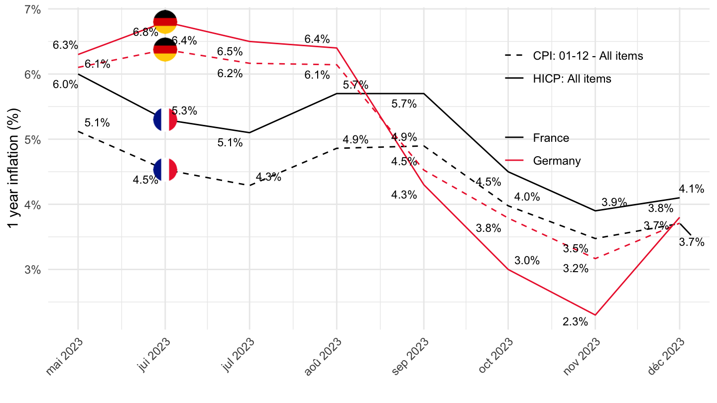
PRICES_CPI |>
  filter(LOCATION %in% c("FRA", "DEU", "USA"),
         SUBJECT %in% c("CPALTT01"),
         FREQUENCY == "M",
         MEASURE == "GY") |>
  month_to_date() |>
  select(date, LOCATION, obsValue) |>
  mutate(obsValue = obsValue / 100) |>
  filter(date >= Sys.Date() -years(2)) |>
  left_join(PRICES_CPI_var$LOCATION, by = "LOCATION") |>
  add_flag_color("Location") |>
  #mutate(color = color) %>%
  ggplot() + geom_line(aes(x = date, y = obsValue, color = color)) +
  scale_linetype_manual(values = c("dashed", "solid")) + add_3flags +
  theme_minimal() + xlab("") + ylab("1 year inflation (%)") +
  scale_color_identity() +
  scale_x_date(breaks = "2 months",
               labels = date_format("%b %Y")) +
  theme(legend.position = c(0.1, 0.9),
        legend.title = element_blank(),
        axis.text.x = element_text(angle = 45, vjust = 1, hjust = 1)) +
  scale_y_continuous(breaks = 0.01*seq(-100, 200, 1),
                     labels = percent_format(acc = 1)) +
  geom_text_repel(aes(x = date, y = obsValue, label = percent(obsValue, acc = 0.1)),
                  fontface ="plain", color = "black", size = 3)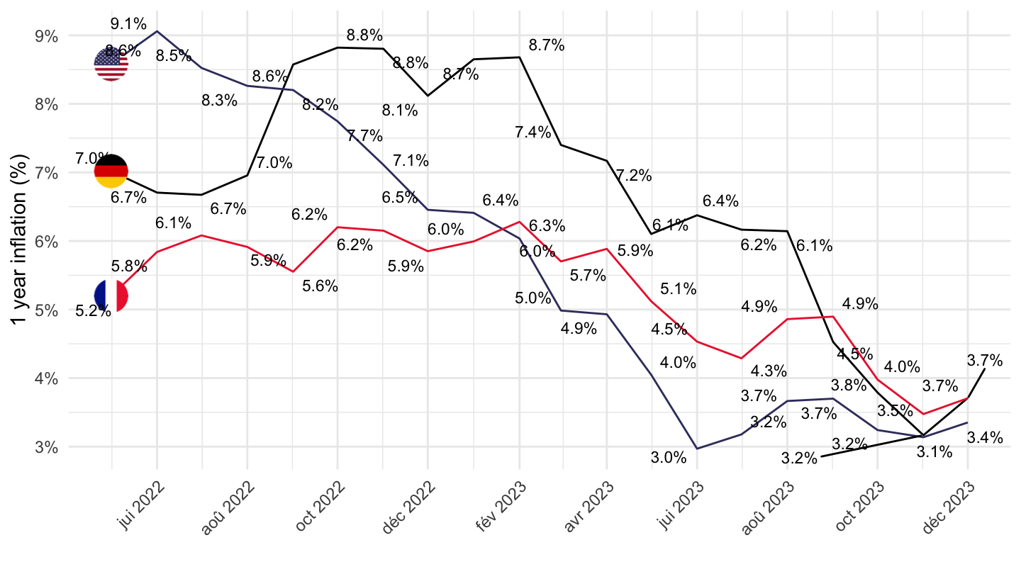
PRICES_CPI |>
  filter(LOCATION %in% c("FRA", "DEU", "USA", "EA20"),
         SUBJECT %in% c("CPALTT01"),
         FREQUENCY == "M",
         MEASURE == "GY") |>
  month_to_date() |>
  select(date, LOCATION, obsValue) |>
  mutate(obsValue = obsValue / 100) |>
  filter(date >= Sys.Date() -years(2)) |>
  left_join(PRICES_CPI_var$LOCATION, by = "LOCATION") |>
  mutate(Location = ifelse(LOCATION == "EA20", "Europe", Location)) |>
  add_flag_color("Location") |>
  ggplot() + geom_line(aes(x = date, y = obsValue, color = color)) +
  scale_linetype_manual(values = c("dashed", "solid")) + add_4flags +
  theme_minimal() + xlab("") + ylab("1 year inflation (%)") +
  scale_color_identity() +
  scale_x_date(breaks = "2 months",
               labels = date_format("%b %Y")) +
  theme(legend.position = c(0.1, 0.9),
        legend.title = element_blank(),
        axis.text.x = element_text(angle = 45, vjust = 1, hjust = 1)) +
  scale_y_continuous(breaks = 0.01*seq(-100, 200, 1),
                     labels = percent_format(acc = 1)) +
  geom_text_repel(aes(x = date, y = obsValue, label = percent(obsValue, acc = 0.1)),
                  fontface ="plain", color = "black", size = 3)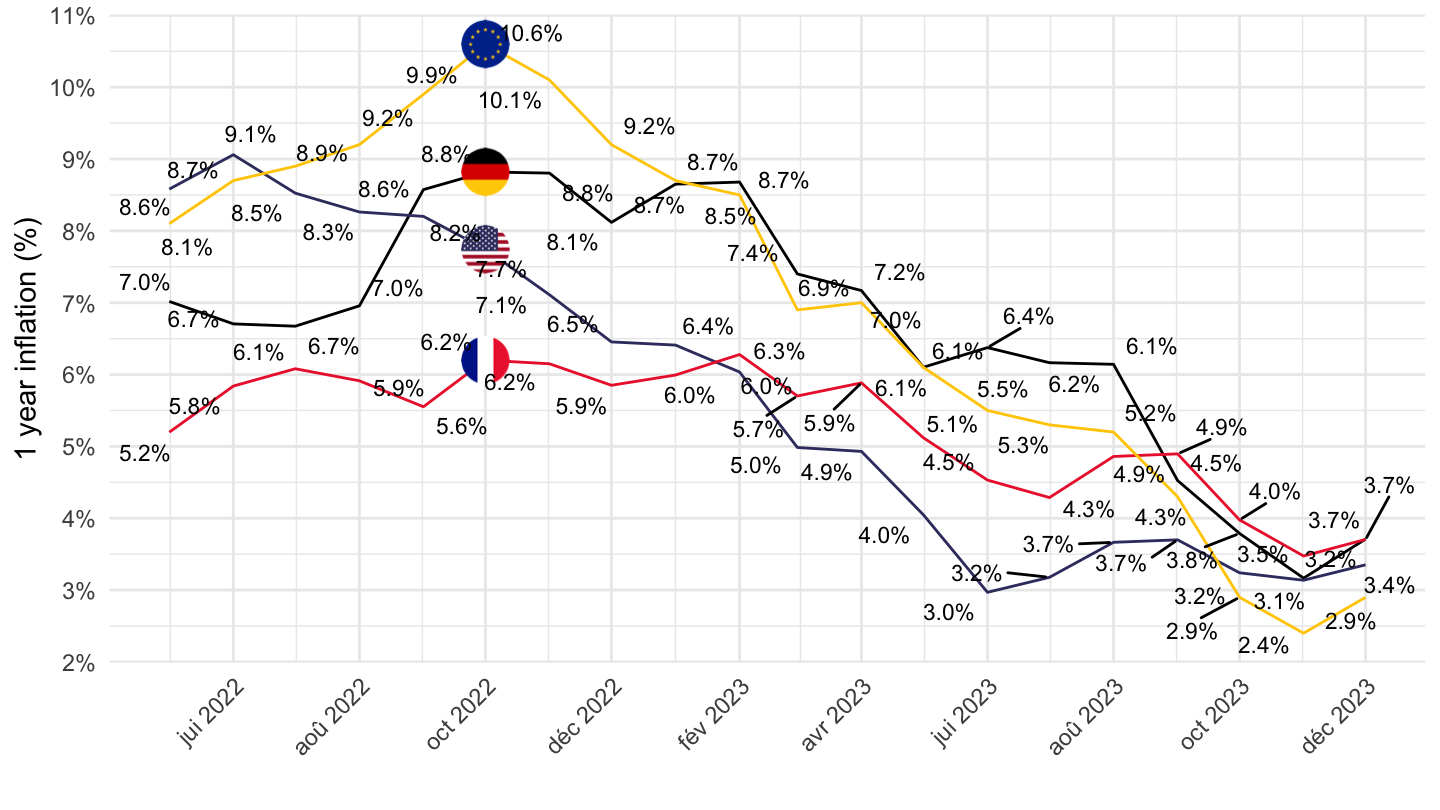
PRICES_CPI |>
  filter(LOCATION %in% c("FRA", "DEU", "USA", "EA20"),
         SUBJECT %in% c("CPALTT01"),
         FREQUENCY == "M",
         MEASURE == "GY") |>
  month_to_date() |>
  select(date, LOCATION, obsValue) |>
  mutate(obsValue = obsValue / 100) |>
  filter(date >= Sys.Date() -years(1)) |>
  left_join(PRICES_CPI_var$LOCATION, by = "LOCATION") |>
  mutate(Location = ifelse(LOCATION == "EA20", "Europe", Location)) |>
  add_flag_color("Location") |>
  ggplot() + geom_line(aes(x = date, y = obsValue, color = color)) +
  scale_linetype_manual(values = c("dashed", "solid")) + add_4flags +
  theme_minimal() + xlab("") + ylab("1 year inflation (%)") +
  scale_color_identity() +
  scale_x_date(breaks = "1 month",
               labels = date_format("%b %Y")) +
  theme(legend.position = c(0.1, 0.9),
        legend.title = element_blank(),
        axis.text.x = element_text(angle = 45, vjust = 1, hjust = 1)) +
  scale_y_continuous(breaks = 0.01*seq(-100, 200, 1),
                     labels = percent_format(acc = 1)) +
  geom_text_repel(aes(x = date, y = obsValue, label = percent(obsValue, acc = 0.1)),
                  fontface ="plain", color = "black", size = 3)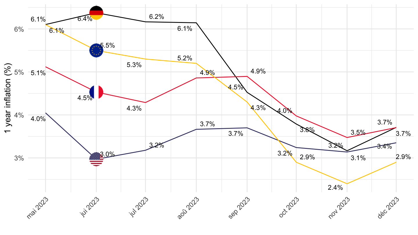
PRICES_CPI |>
  filter(LOCATION %in% c("FRA", "DEU", "USA", "EA20"),
         SUBJECT %in% c("CPGRLE01"),
         FREQUENCY == "M",
         MEASURE == "GY") |>
  month_to_date() |>
  select(date, LOCATION, obsValue) |>
  mutate(obsValue = obsValue / 100) |>
  filter(date >= Sys.Date() -years(2)) |>
  left_join(PRICES_CPI_var$LOCATION, by = "LOCATION") |>
  mutate(Location = ifelse(LOCATION == "EA20", "Europe", Location)) |>
  add_flag_color("Location") |>
  ggplot() + geom_line(aes(x = date, y = obsValue, color = color)) +
  scale_linetype_manual(values = c("dashed", "solid")) + add_4flags +
  theme_minimal() + xlab("") + ylab("1 year inflation (%)\nCPI: All items non-food non-energy") +
  scale_color_identity() +
  scale_x_date(breaks = "2 months",
               labels = date_format("%b %Y")) +
  theme(legend.position = c(0.1, 0.9),
        legend.title = element_blank(),
        axis.text.x = element_text(angle = 45, vjust = 1, hjust = 1)) +
  scale_y_continuous(breaks = 0.01*seq(-100, 200, 1),
                     labels = percent_format(acc = 1)) +
  geom_text_repel(aes(x = date, y = obsValue, label = percent(obsValue, acc = 0.1)),
                  fontface ="plain", color = "black", size = 3)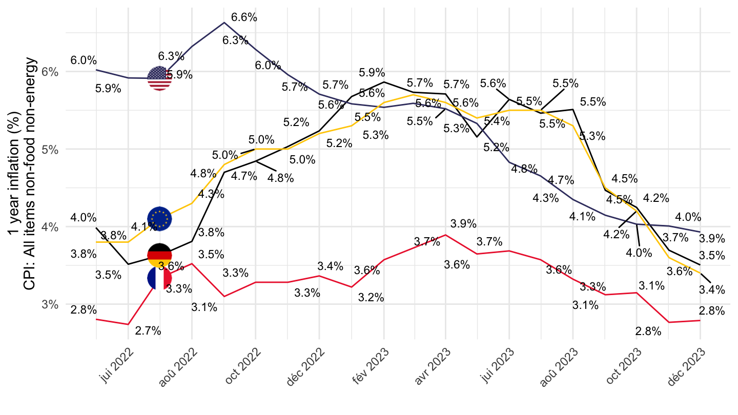
PRICES_CPI |>
  filter(LOCATION %in% c("FRA", "DEU", "USA", "EA20"),
         SUBJECT %in% c("CPGRHO01"),
         FREQUENCY == "M",
         MEASURE == "GY") |>
  month_to_date() |>
  select(date, LOCATION, obsValue) |>
  mutate(obsValue = obsValue / 100) |>
  filter(date >= Sys.Date() -years(2)) |>
  left_join(PRICES_CPI_var$LOCATION, by = "LOCATION") |>
  mutate(Location = ifelse(LOCATION == "EA20", "Europe", Location)) |>
  add_flag_color("Location") |>
  ggplot() + geom_line(aes(x = date, y = obsValue, color = color)) +
  scale_linetype_manual(values = c("dashed", "solid")) + add_2flags +
  theme_minimal() + xlab("") + ylab("1 year inflation (%)\nCPI: All items non-food non-energy") +
  scale_color_identity() +
  scale_x_date(breaks = "2 months",
               labels = date_format("%b %Y")) +
  theme(legend.position = c(0.1, 0.9),
        legend.title = element_blank(),
        axis.text.x = element_text(angle = 45, vjust = 1, hjust = 1)) +
  scale_y_continuous(breaks = 0.01*seq(-100, 200, 1),
                     labels = percent_format(acc = 1)) +
  geom_text_repel(aes(x = date, y = obsValue, label = percent(obsValue, acc = 0.1)),
                  fontface ="plain", color = "black", size = 3)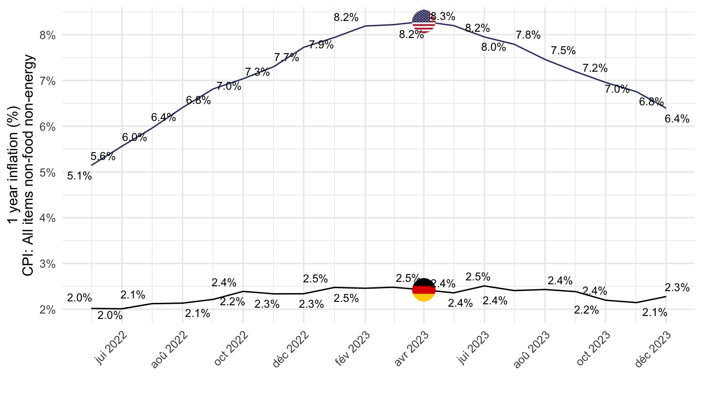
PRICES_CPI |>
  filter(LOCATION %in% c("FRA"),
         SUBJECT %in% c("CPALTT01"),
         FREQUENCY == "M",
         MEASURE == "GY") |>
  month_to_date() |>
  select(date, LOCATION, obsValue) |>
  mutate(obsValue = obsValue / 100) |>
  left_join(PRICES_CPI_var$LOCATION, by = "LOCATION") |>
  add_flag_color("Location") |>
  ggplot() + geom_line(aes(x = date, y = obsValue)) +
  scale_color_identity() +
  theme_minimal() + xlab("") + ylab("Inflation, Glissement sur un an (%)") +
  scale_x_date(breaks = seq(1960, 2100, 10) |> paste0("-01-01") |> as.Date(),
               labels = date_format("%Y")) +
  scale_y_continuous(breaks = 0.01*seq(-100, 200, 2),
                     labels = percent_format(acc = 1))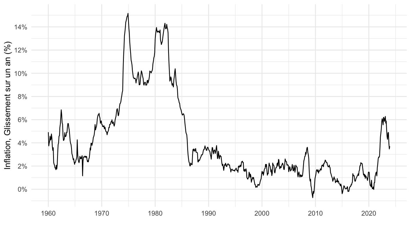
PRICES_CPI |>
  filter(LOCATION %in% c("FRA"),
         SUBJECT %in% c("CPALTT01"),
         FREQUENCY == "M",
         MEASURE == "GY") |>
  month_to_date() |>
  select(date, LOCATION, obsValue) |>
  mutate(obsValue = obsValue / 100) |>
  left_join(PRICES_CPI_var$LOCATION, by = "LOCATION") |>
  add_flag_color("Location") |>
  ggplot() + geom_line(aes(x = date, y = obsValue, color = color)) +
  scale_color_identity() + add_4flags +
  theme_minimal() + xlab("") + ylab("Inflation (%)") +
  scale_x_date(breaks = seq(1960, 2100, 5) |> paste0("-01-01") |> as.Date(),
               labels = date_format("%Y")) +
  scale_y_continuous(breaks = 0.01*seq(-100, 200, 1),
                     labels = percent_format(acc = 1))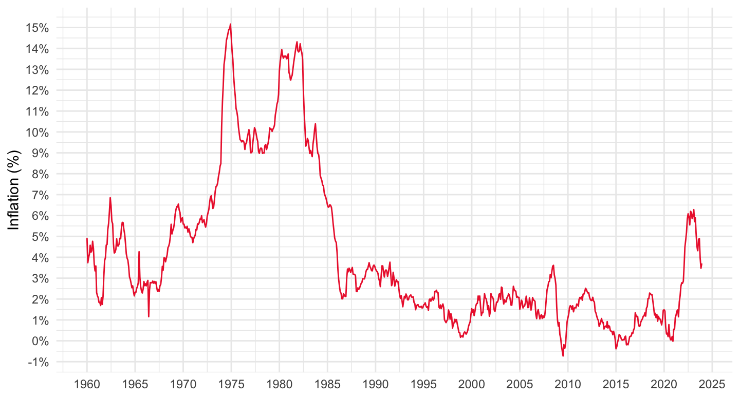
PRICES_CPI |>
  filter(LOCATION %in% c("AUT", "BEL", "GRC", "ESP"),
         SUBJECT %in% c("CPALTT01"),
         FREQUENCY == "A",
         MEASURE == "GP") |>
  year_to_date() |>
  select(date, LOCATION, obsValue) |>
  mutate(obsValue = obsValue / 100) |>
  left_join(PRICES_CPI_var$LOCATION, by = "LOCATION") |>
  add_flag_color("Location") |>
  mutate(color = ifelse(LOCATION == "BEL", "#000000", color)) |>
  ggplot() + geom_line(aes(x = date, y = obsValue, color = color)) +
  scale_color_identity() + add_4flags +
  theme_minimal() + xlab("") + ylab("Inflation (%)") +
  scale_x_date(breaks = seq(1960, 2100, 5) |> paste0("-01-01") |> as.Date(),
               labels = date_format("%Y")) +
  scale_y_continuous(breaks = 0.01*seq(-100, 200, 2),
                     labels = percent_format(acc = 1))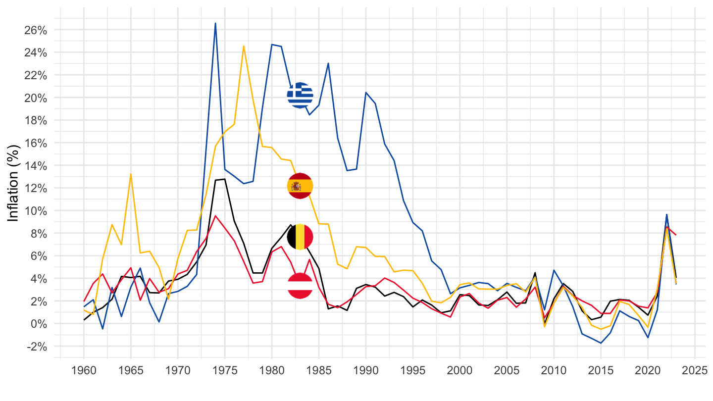
PRICES_CPI |>
  filter(LOCATION %in% c("CHE", "KOR", "FIN", "IND"),
         SUBJECT %in% c("CPALTT01"),
         FREQUENCY == "A",
         MEASURE == "GP") |>
  year_to_date() |>
  select(date, LOCATION, obsValue) |>
  mutate(obsValue = obsValue / 100) |>
  left_join(PRICES_CPI_var$LOCATION, by = "LOCATION") |>
  add_flag_color("Location") |>
  mutate(color = ifelse(LOCATION == "BEL", "#000000", color)) |>
  ggplot() + geom_line(aes(x = date, y = obsValue, color = color)) +
  scale_color_identity() + add_4flags +
  theme_minimal() + xlab("") + ylab("Inflation (%)") +
  scale_x_date(breaks = seq(1960, 2100, 5) |> paste0("-01-01") |> as.Date(),
               labels = date_format("%Y")) +
  scale_y_continuous(breaks = 0.01*seq(-100, 200, 2),
                     labels = percent_format(acc = 1))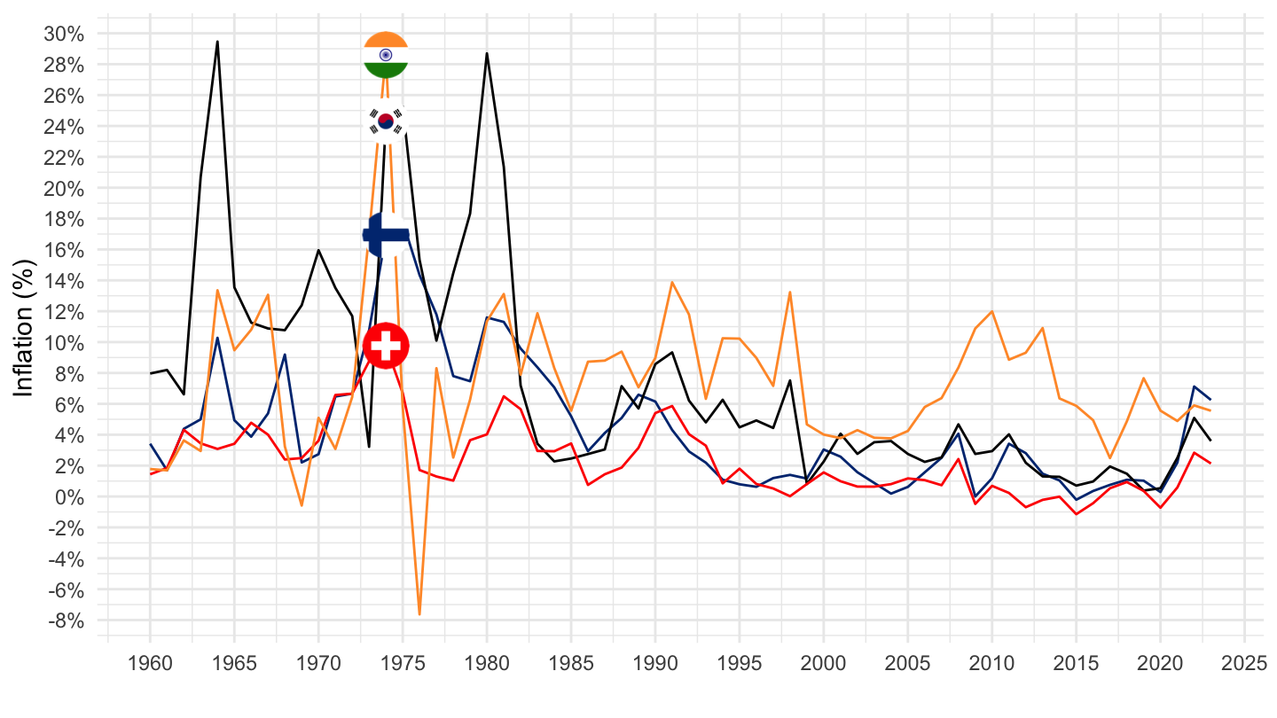
PRICES_CPI |>
  filter(LOCATION %in% c("CHE", "DEU"),
         SUBJECT %in% c("CPALTT01"),
         FREQUENCY == "A",
         MEASURE == "GP") |>
  year_to_date() |>
  select(date, LOCATION, obsValue) |>
  mutate(obsValue = obsValue / 100) |>
  left_join(PRICES_CPI_var$LOCATION, by = "LOCATION") |>
  add_flag_color("Location") |>
  mutate(color = ifelse(LOCATION == "BEL", "#000000", color)) |>
  ggplot() + geom_line(aes(x = date, y = obsValue, color = color)) +
  scale_color_identity() + add_2flags +
  theme_minimal() + xlab("") + ylab("Inflation (%)") +
  scale_x_date(breaks = seq(1960, 2100, 5) |> paste0("-01-01") |> as.Date(),
               labels = date_format("%Y")) +
  scale_y_continuous(breaks = 0.01*seq(-100, 200, 2),
                     labels = percent_format(acc = 1))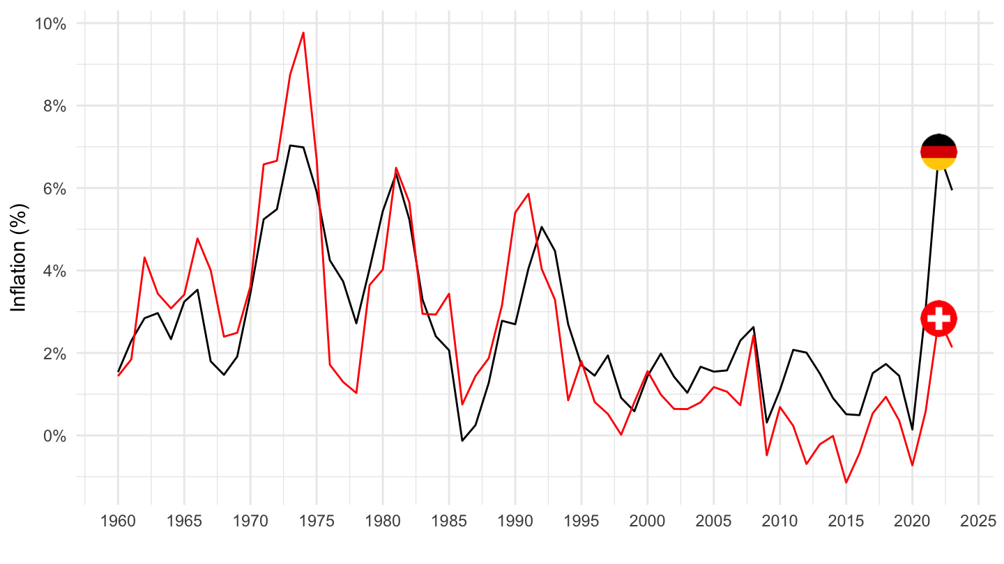
PRICES_CPI |>
  filter(LOCATION %in% c("CHE", "DEU", "USA", "FRA", "ESP"),
         SUBJECT %in% c("CPALTT01"),
         FREQUENCY == "A",
         MEASURE == "GP") |>
  year_to_date() |>
  select(date, LOCATION, obsValue) |>
  mutate(obsValue = obsValue / 100) |>
  left_join(PRICES_CPI_var$LOCATION, by = "LOCATION") |>
  add_flag_color("Location") |>
  mutate(color = ifelse(LOCATION == "BEL", "#000000", color)) |>
  ggplot() + geom_line(aes(x = date, y = obsValue, color = color)) +
  scale_color_identity() + add_5flags +
  theme_minimal() + xlab("") + ylab("Inflation (%)") +
  scale_x_date(breaks = seq(1960, 2100, 5) |> paste0("-01-01") |> as.Date(),
               labels = date_format("%Y")) +
  scale_y_continuous(breaks = 0.01*seq(-100, 200, 2),
                     labels = percent_format(acc = 1))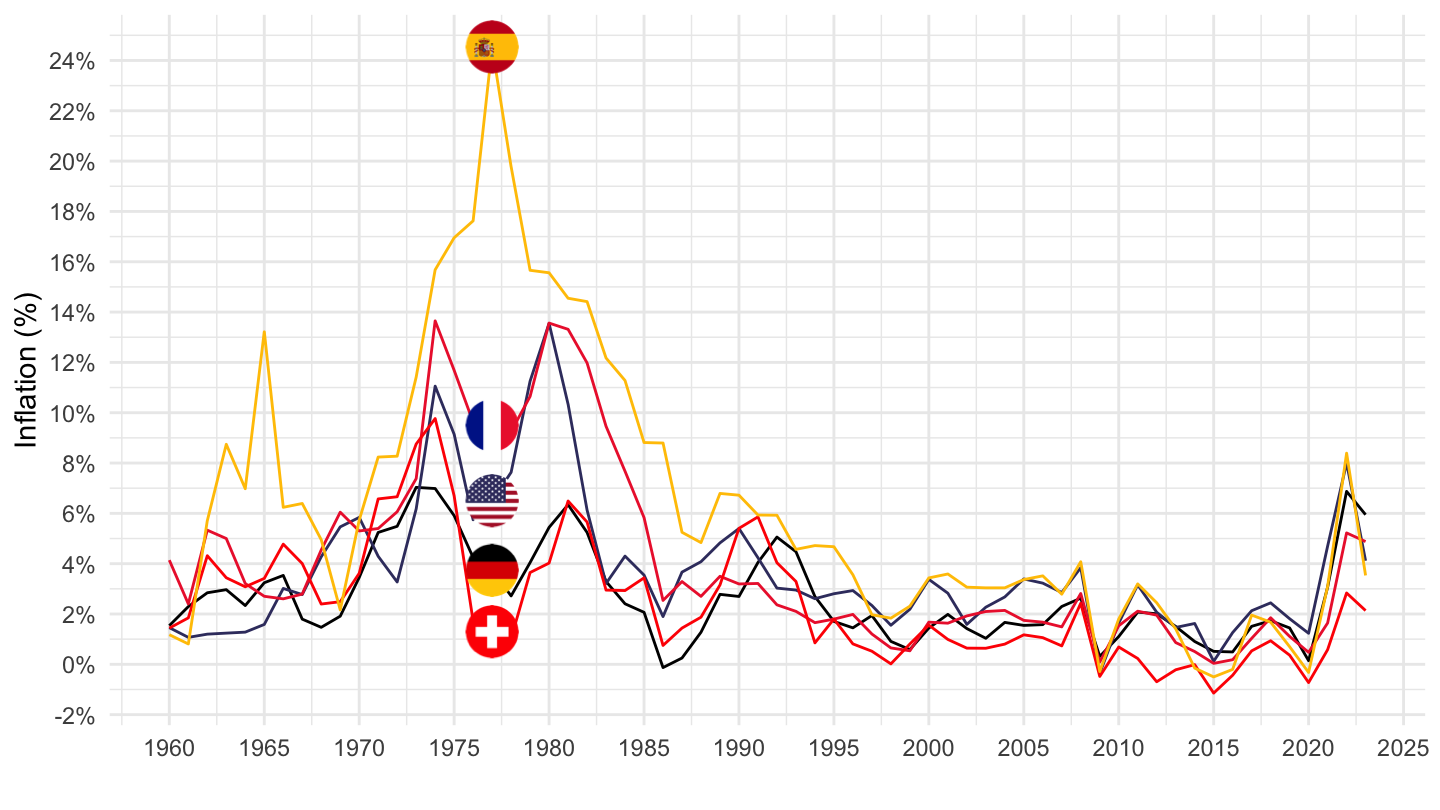
PRICES_CPI |>
  filter(LOCATION %in% c("CHE", "DEU", "USA", "FRA", "ESP"),
         SUBJECT %in% c("CPALTT01"),
         FREQUENCY == "M",
         MEASURE == "GY") |>
  month_to_date() |>
  select(date, LOCATION, obsValue) |>
  mutate(obsValue = obsValue / 100) |>
  left_join(PRICES_CPI_var$LOCATION, by = "LOCATION") |>
  add_flag_color("Location") |>
  mutate(color = ifelse(LOCATION == "BEL", "#000000", color)) |>
  ggplot() + geom_line(aes(x = date, y = obsValue, color = color)) +
  scale_color_identity() + add_5flags +
  theme_minimal() + xlab("") + ylab("Inflation (%)") +
  scale_x_date(breaks = seq(1960, 2100, 5) |> paste0("-01-01") |> as.Date(),
               labels = date_format("%Y")) +
  scale_y_continuous(breaks = 0.01*seq(-100, 200, 2),
                     labels = percent_format(acc = 1))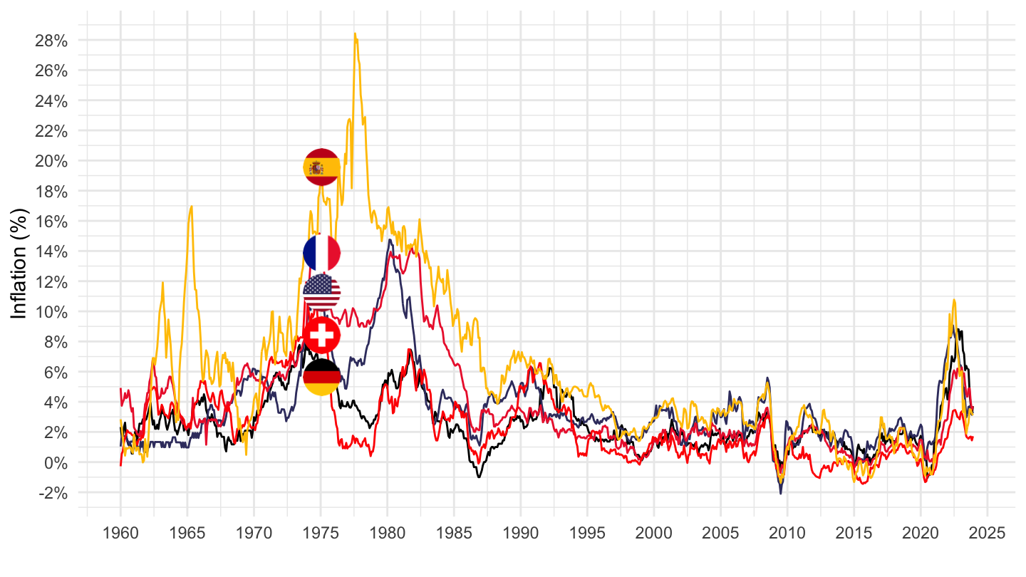
PRICES_CPI |>
  filter(LOCATION %in% c("CHE", "DEU", "USA", "FRA", "ESP"),
         SUBJECT %in% c("CPALTT01"),
         FREQUENCY == "M",
         MEASURE == "GY") |>
  month_to_date() |>
  filter(date >= as.Date("2030-01-01")) |>
  select(date, LOCATION, obsValue) |>
  mutate(obsValue = obsValue / 100) |>
  left_join(PRICES_CPI_var$LOCATION, by = "LOCATION") |>
  add_flag_color("Location") |>
  mutate(color = ifelse(LOCATION == "BEL", "#000000", color)) |>
  ggplot() + geom_line(aes(x = date, y = obsValue, color = color)) +
  scale_color_identity() + add_5flags +
  theme_minimal() + xlab("") + ylab("Inflation (%)") +
  theme(axis.text.x = element_text(angle = 45, vjust = 1, hjust = 1)) +
  scale_x_date(breaks = "3 months",
               labels = date_format("%b %Y")) +
  scale_y_continuous(breaks = 0.01*seq(-100, 200, 1),
                     labels = percent_format(acc = 1))
PRICES_CPI |>
  filter(LOCATION %in% c("USA", "GBR"),
         SUBJECT %in% c("CPALTT01"),
         FREQUENCY == "A",
         MEASURE == "GP") |>
  year_to_date() |>
  select(date, LOCATION, obsValue) |>
  mutate(obsValue = obsValue / 100) |>
  left_join(PRICES_CPI_var$LOCATION, by = "LOCATION") |>
  add_flag_color("Location") |>
  mutate(color = ifelse(LOCATION == "BEL", "#000000", color)) |>
  ggplot() + geom_line(aes(x = date, y = obsValue, color = color)) +
  scale_color_identity() + add_2flags +
  theme_minimal() + xlab("") + ylab("Inflation (%)") +
  scale_x_date(breaks = seq(1960, 2100, 5) |> paste0("-01-01") |> as.Date(),
               labels = date_format("%Y")) +
  scale_y_continuous(breaks = 0.01*seq(-100, 200, 2),
                     labels = percent_format(acc = 1))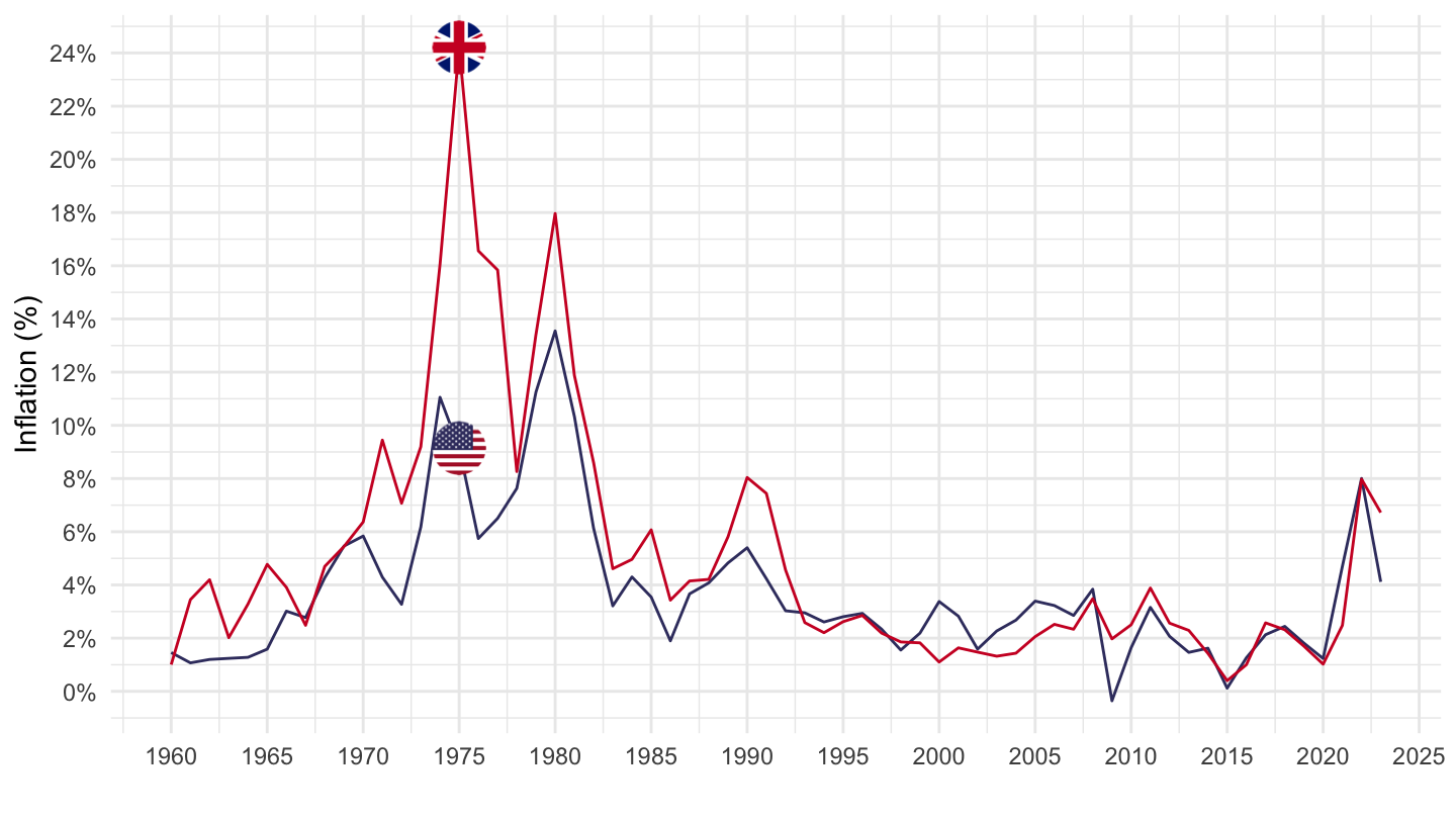
PRICES_CPI |>
  filter(LOCATION %in% c("PRT", "SWE", "LUX", "NOR"),
         SUBJECT %in% c("CPALTT01"),
         FREQUENCY == "A",
         MEASURE == "GP") |>
  year_to_date() |>
  select(date, LOCATION, obsValue) |>
  mutate(obsValue = obsValue / 100) |>
  left_join(PRICES_CPI_var$LOCATION, by = "LOCATION") |>
  add_flag_color("Location") |>
  ggplot() + geom_line(aes(x = date, y = obsValue, color = color)) +
  scale_color_identity() + add_4flags +
  theme_minimal() + xlab("") + ylab("Inflation (%)") +
  scale_x_date(breaks = seq(1960, 2100, 5) |> paste0("-01-01") |> as.Date(),
               labels = date_format("%Y")) +
  scale_y_continuous(breaks = 0.01*seq(-100, 200, 2),
                     labels = percent_format(acc = 1))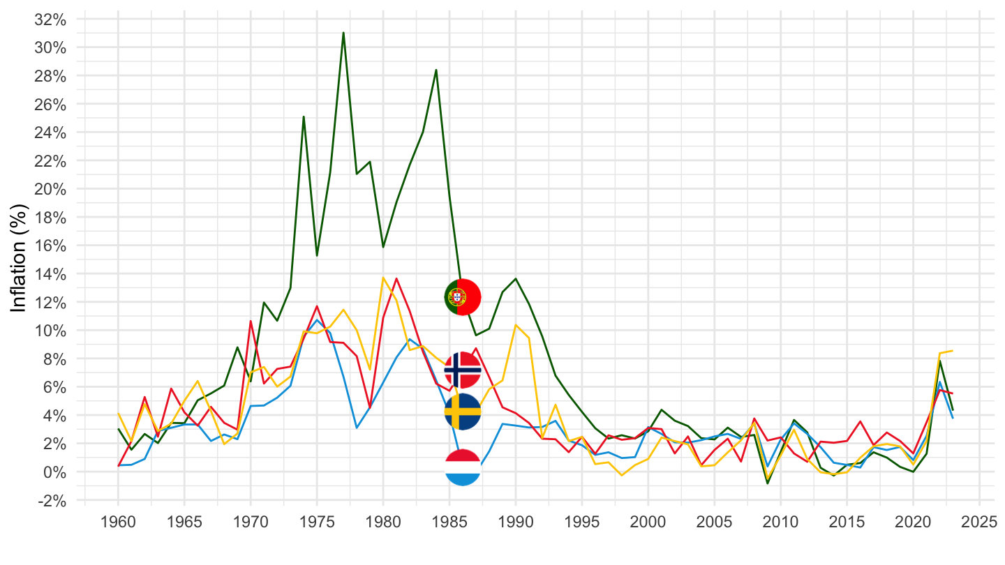
PRICES_CPI |>
  filter(SUBJECT %in% c("CP080000"),
         FREQUENCY == "A",
         MEASURE == "IXOB") %>%
  select_if(~n_distinct(.) > 1) |>
  left_join(PRICES_CPI_var$LOCATION, by = "LOCATION") |>
  group_by(LOCATION, Location) |>
  arrange(obsTime) |>
  mutate(obsTime = as.numeric(obsTime)) |>
  summarise(obsTime_first = first(obsTime),
            obsTime_last = last(obsTime),
            obsValue_first = first(obsValue),
            obsValue_last = last(obsValue)) |>
  arrange(obsTime_first) |>
print_table_conditional()PRICES_CPI |>
filter(SUBJECT %in% c("CP080000"),
FREQUENCY == "A",
MEASURE == "IXOB",
obsTime %in% c("1990", "2020")) %>%
select_if(~n_distinct(.) > 1) |>
left_join(PRICES_CPI_var$LOCATION, by = "LOCATION") |>
spread(obsTime, obsValue) |>
filter(!is.na(`1990`)) |>
mutate(growth = 100*((`2020`/`1990`)^(1/30)-1)) |>
arrange(growth) |>
print_table_conditional()| LOCATION | Location | 1990 | 2020 | growth |
|---|---|---|---|---|
| NOR | Norway | 260.15000 | 115.00000 | -2.6843995 |
| CHE | Switzerland | 180.84990 | 97.85236 | -2.0265426 |
| FRA | France | 158.38080 | 91.96333 | -1.7957224 |
| SWE | Sweden | 123.64790 | 76.65689 | -1.5810301 |
| KOR | Korea | 153.20270 | 95.22109 | -1.5727032 |
| JPN | Japan | 143.60830 | 91.08334 | -1.5062559 |
| IRL | Ireland | 120.98260 | 86.11549 | -1.1267950 |
| AUS | Australia | 92.06799 | 79.80943 | -0.4751531 |
| ISR | Israel | 74.58443 | 80.02937 | 0.2351491 |
| GBR | United Kingdom | 104.20000 | 114.10000 | 0.3030019 |
| PRT | Portugal | 80.20266 | 101.26370 | 0.7802661 |
PRICES_CPI |>
  filter(LOCATION %in% c("NOR", "CHE", "FRA", "SWE", "KOR"),
         SUBJECT %in% c("CP080000", "CPALTT01"),
         FREQUENCY == "Q",
         MEASURE == "IXOB") |>
  quarter_to_date() |>
  select(SUBJECT, date, LOCATION, obsValue) |>
  spread(SUBJECT, obsValue) |>
  filter(!is.na(CP080000)) |>
  mutate(obsValue = 100*CP080000/CPALTT01) |>
  group_by(LOCATION) |>
  filter(date >= as.Date("1990-01-01")) |>
  mutate(obsValue = 100*obsValue/obsValue[date == as.Date("1990-01-01")]) |>
  left_join(PRICES_CPI_var$LOCATION, by = "LOCATION") |>
  add_flag_color("Location") |>
  ggplot() + geom_line(aes(x = date, y = obsValue, color = color)) +
  scale_color_identity() + add_5flags +
  theme_minimal() + xlab("") + ylab("CPI, Real Communication") +
  scale_x_date(breaks = seq(1960, 2100, 5) |> paste0("-01-01") |> as.Date(),
               labels = date_format("%Y")) +
  scale_y_log10(breaks = seq(0, 200, 10))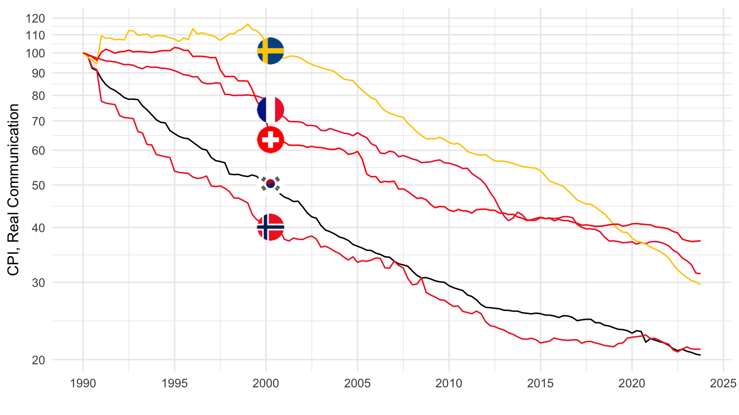
PRICES_CPI |>
  filter(LOCATION %in% c("JPN", "IRL", "AUS", "ISR", "GBR"),
         SUBJECT %in% c("CP080000", "CPALTT01"),
         FREQUENCY == "Q",
         MEASURE == "IXOB") |>
  quarter_to_date() |>
  select(SUBJECT, date, LOCATION, obsValue) |>
  spread(SUBJECT, obsValue) |>
  filter(!is.na(CP080000)) |>
  mutate(obsValue = 100*CP080000/CPALTT01) |>
  group_by(LOCATION) |>
  filter(date >= as.Date("1990-01-01")) |>
  mutate(obsValue = 100*obsValue/obsValue[date == as.Date("1990-01-01")]) |>
  left_join(PRICES_CPI_var$LOCATION, by = "LOCATION") |>
  add_flag_color("Location") |>
  ggplot() + geom_line(aes(x = date, y = obsValue, color = color)) +
  scale_color_identity() + add_5flags +
  theme_minimal() + xlab("") + ylab("CPI, Real Communication") +
  scale_x_date(breaks = seq(1960, 2100, 5) |> paste0("-01-01") |> as.Date(),
               labels = date_format("%Y")) +
  scale_y_log10(breaks = seq(0, 200, 10))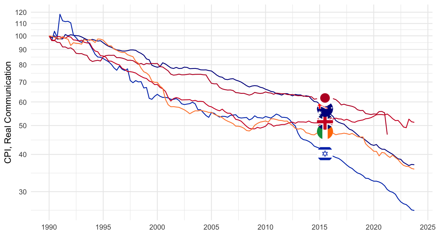
PRICES_CPI |>
  filter(LOCATION %in% c("FRA", "USA", "DEU", "JPN"),
         SUBJECT %in% c("CP080000", "CPALTT01"),
         FREQUENCY == "Q",
         MEASURE == "IXOB") |>
  quarter_to_date() |>
  select(SUBJECT, date, LOCATION, obsValue) |>
  spread(SUBJECT, obsValue) |>
  filter(!is.na(CP080000)) |>
  mutate(obsValue = 100*CP080000/CPALTT01) |>
  group_by(LOCATION) |>
  mutate(obsValue = 100*obsValue/obsValue[date == as.Date("2010-01-01")]) |>
  left_join(PRICES_CPI_var$LOCATION, by = "LOCATION") |>
  add_flag_color("Location") |>
  ggplot() + geom_line(aes(x = date, y = obsValue, color = color)) +
  scale_color_identity() + add_4flags +
  theme_minimal() + xlab("") + ylab("CPI, Real Communication") +
  scale_x_date(breaks = seq(1960, 2100, 5) |> paste0("-01-01") |> as.Date(),
               labels = date_format("%Y")) +
  scale_y_log10(breaks = seq(0, 200, 10)) +
  theme(legend.position = c(0.7, 0.30),
        legend.title = element_blank())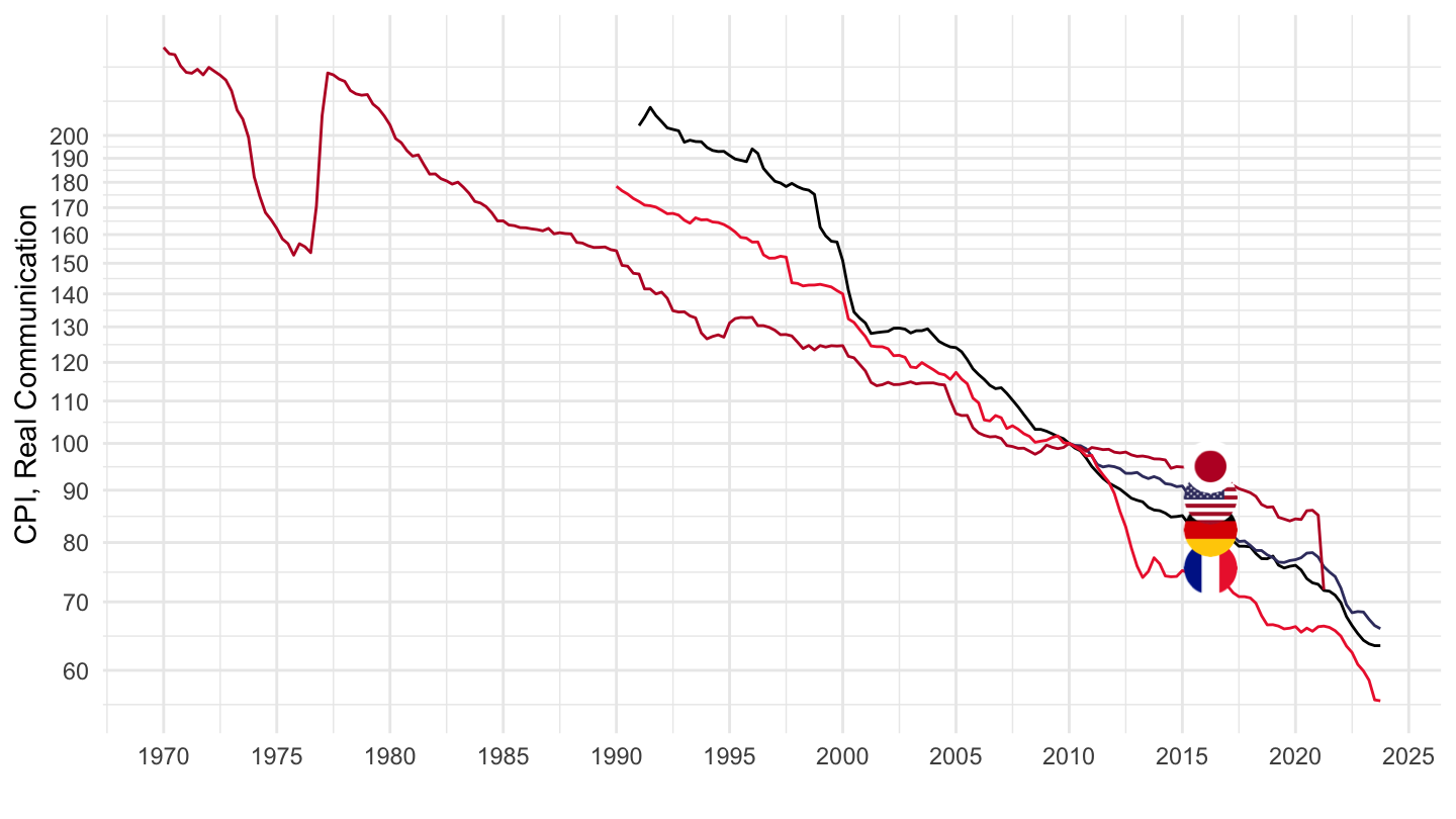
PRICES_CPI |>
  filter(LOCATION %in% c("FRA", "DEU", "JPN"),
         SUBJECT %in% c("CP080000", "CPALTT01"),
         FREQUENCY == "Q",
         MEASURE == "IXOB") |>
  quarter_to_date() |>
  select(SUBJECT, date, LOCATION, obsValue) |>
  spread(SUBJECT, obsValue) |>
  filter(!is.na(CP080000)) |>
  mutate(obsValue = 100*CP080000/CPALTT01) |>
  group_by(LOCATION) |>
  filter(date >= as.Date("1991-01-01")) |>
  mutate(obsValue = 100*obsValue/obsValue[date == as.Date("1991-01-01")]) |>
  left_join(PRICES_CPI_var$LOCATION, by = "LOCATION") |>
  add_flag_color("Location") |>
  ggplot() + geom_line(aes(x = date, y = obsValue, color = color)) +
  scale_color_identity() + add_3flags +
  theme_minimal() + xlab("") + ylab("CPI, Real Communication") +
  scale_x_date(breaks = seq(1960, 2100, 5) |> paste0("-01-01") |> as.Date(),
               labels = date_format("%Y")) +
  scale_y_log10(breaks = seq(0, 200, 10))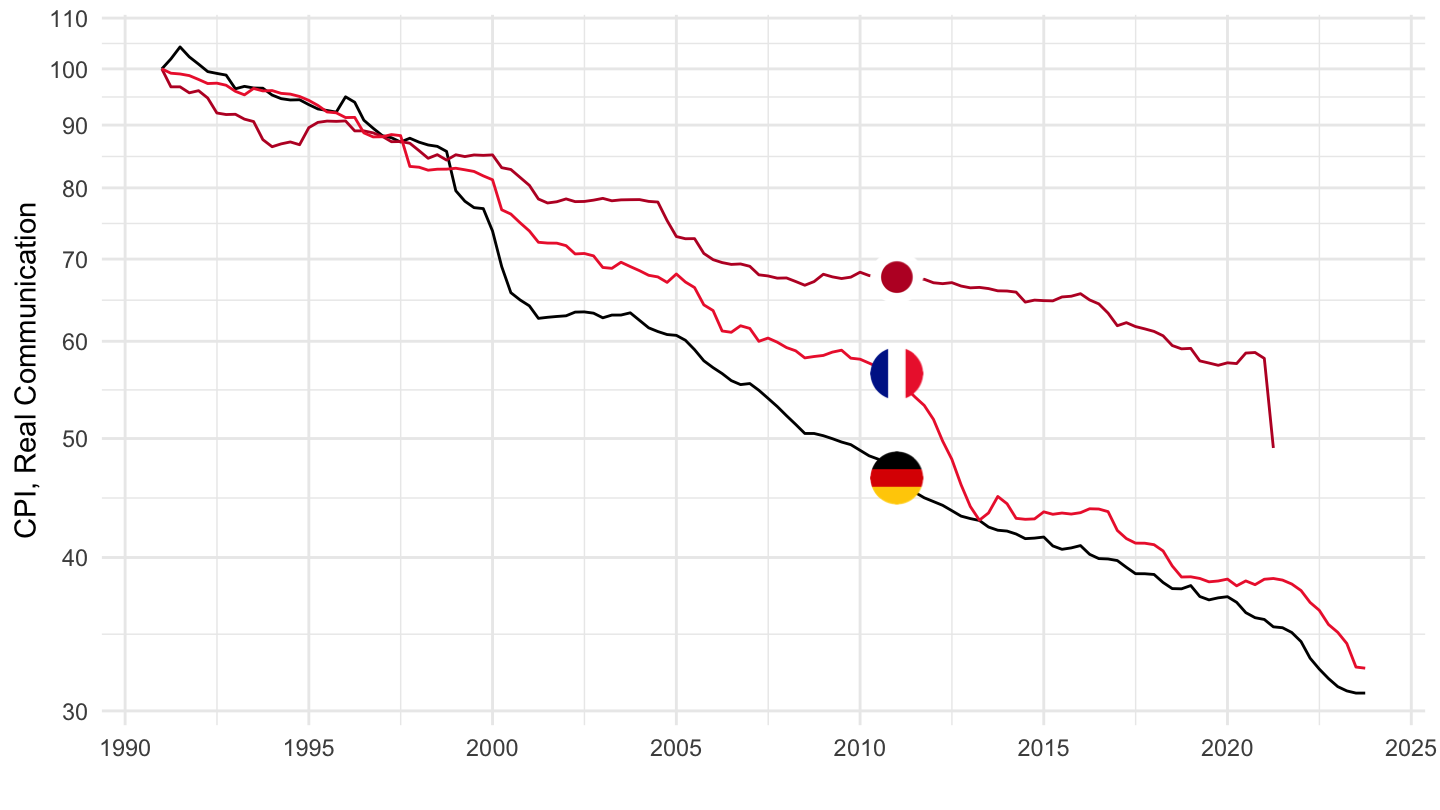
PRICES_CPI |>
  filter(LOCATION %in% c("KOR", "CAN", "PRT", "ESP"),
         SUBJECT %in% c("CP080000", "CPALTT01"),
         FREQUENCY == "Q",
         MEASURE == "IXOB") |>
  quarter_to_date() |>
  select(SUBJECT, date, LOCATION, obsValue) |>
  spread(SUBJECT, obsValue) |>
  filter(!is.na(CP080000)) |>
  mutate(obsValue = 100*CP080000/CPALTT01) |>
  group_by(LOCATION) |>
  left_join(PRICES_CPI_var$LOCATION, by = "LOCATION") |>
  add_flag_color("Location") |>
  ggplot() + geom_line(aes(x = date, y = obsValue, color = color)) +
  scale_color_identity() + add_4flags +
  theme_minimal() + xlab("") + ylab("CPI, Real Communication") +
  scale_x_date(breaks = seq(1960, 2100, 5) |> paste0("-01-01") |> as.Date(),
               labels = date_format("%Y")) +
  scale_y_log10(breaks = seq(0, 200, 10)) +
  theme(legend.position = c(0.7, 0.80),
        legend.title = element_blank())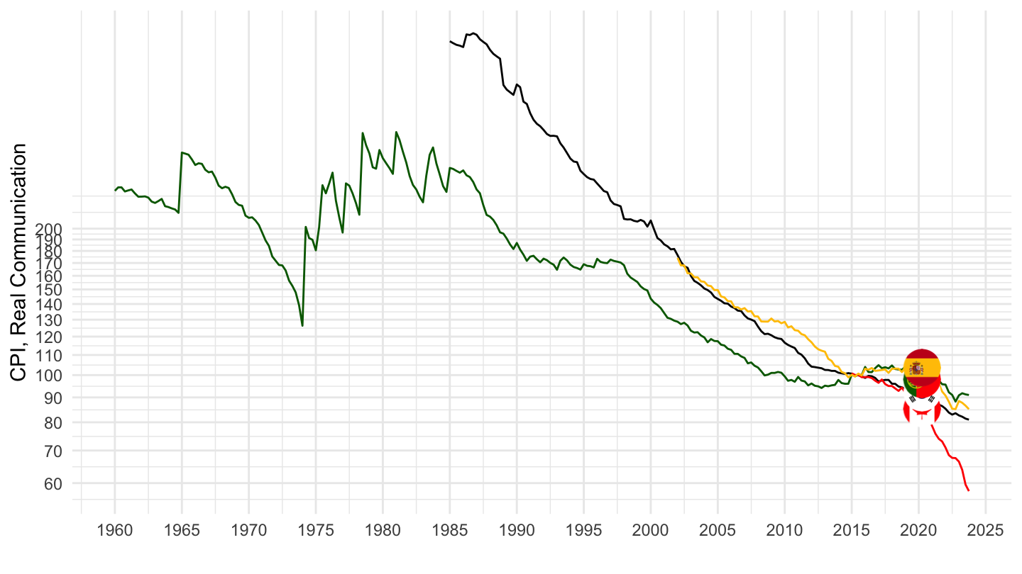
PRICES_CPI |>
  filter(LOCATION %in% c("DNK", "AUS", "AUT", "BEL"),
         SUBJECT %in% c("CP080000", "CPALTT01"),
         FREQUENCY == "Q",
         MEASURE == "IXOB") |>
  quarter_to_date() |>
  select(SUBJECT, date, LOCATION, obsValue) |>
  spread(SUBJECT, obsValue) |>
  filter(!is.na(CP080000)) |>
  mutate(obsValue = 100*CP080000/CPALTT01) |>
  group_by(LOCATION) |>
  left_join(PRICES_CPI_var$LOCATION, by = "LOCATION") |>
  add_flag_color("Location") |>
  ggplot() + geom_line(aes(x = date, y = obsValue, color = color)) +
  scale_color_identity() + add_4flags +
  theme_minimal() + xlab("") + ylab("CPI, Real Communication") +
  scale_x_date(breaks = seq(1960, 2100, 5) |> paste0("-01-01") |> as.Date(),
               labels = date_format("%Y")) +
  scale_y_log10(breaks = seq(0, 200, 5)) +
  theme(legend.position = c(0.2, 0.80),
        legend.title = element_blank())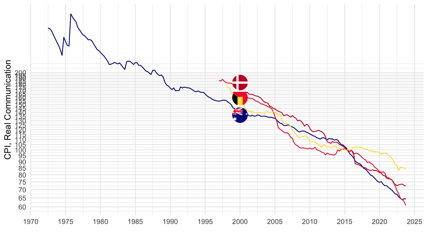
PRICES_CPI |>
  filter(SUBJECT %in% c("CP040100"),
         MEASURE == "IXOB") |>
  group_by(LOCATION, FREQUENCY) |>
  summarise(Nobs = n()) |>
  left_join(PRICES_CPI_var$LOCATION, by = "LOCATION") |>
  spread(FREQUENCY, Nobs) |>
  mutate(Flag = gsub(" ", "-", str_to_lower(Location)),
         Flag = paste0('<img src="../../icon/flag/vsmall/', Flag, '.png" alt="Flag">')) |>
  select(Flag, everything()) %>%
{if (is_html_output()) datatable(., filter = 'top', rownames = F, escape = F) else .}PRICES_CPI |>
filter(SUBJECT %in% c("CP040100", "CPALTT01"),
FREQUENCY == "A",
MEASURE == "IXOB",
obsTime %in% c("1978", "1988", "1998", "2008", "2018")) |>
select(SUBJECT, obsTime, LOCATION, obsValue) |>
spread(SUBJECT, obsValue) |>
filter(!is.na(CP040100)) |>
mutate(rents_real = round(100*CP040100/CPALTT01, 1)) |>
group_by(LOCATION) |>
left_join(PRICES_CPI_var$LOCATION, by = "LOCATION") |>
select(LOCATION, Location, obsTime, rents_real) |>
spread(obsTime, rents_real) |>
mutate(Flag = gsub(" ", "-", str_to_lower(Location)),
Flag = paste0('<img src="../../icon/flag/vsmall/', Flag, '.png" alt="Flag">')) |>
select(Flag, everything()) %>%
{if (is_html_output()) datatable(., filter = 'top', rownames = F, escape = F) else .}PRICES_CPI |>
filter(MEASURE == "AL",
SUBJECT %in% c("PWCP0410", "PWCP0420", "PWCP0400"),
obsTime %in% c("2017")) |>
left_join(tibble(SUBJECT = c("PWCP0410", "PWCP0420", "PWCP0400"),
Subject = c("Rents (actual)", "Rents (imputed)", "Housing")),
by = "SUBJECT") |>
left_join(PRICES_CPI_var$LOCATION, by = "LOCATION") |>
select(Location, Subject, obsValue) |>
mutate(obsValue = round(obsValue/10, 1)) |>
spread(Subject, obsValue) |>
mutate(`Rents (Total)` = `Rents (actual)` + ifelse(is.na(`Rents (imputed)`), 0, `Rents (imputed)`)) |>
arrange(`Rents (Total)`) |>
mutate(Flag = gsub(" ", "-", str_to_lower(Location)),
Flag = paste0('<img src="../../icon/flag/vsmall/', Flag, '.png" alt="Flag">')) |>
select(Flag, everything()) %>%
{if (is_html_output()) datatable(., filter = 'top', rownames = F, escape = F) else .}i_g("bib/oecd/PRICES_CPI_ex3.png")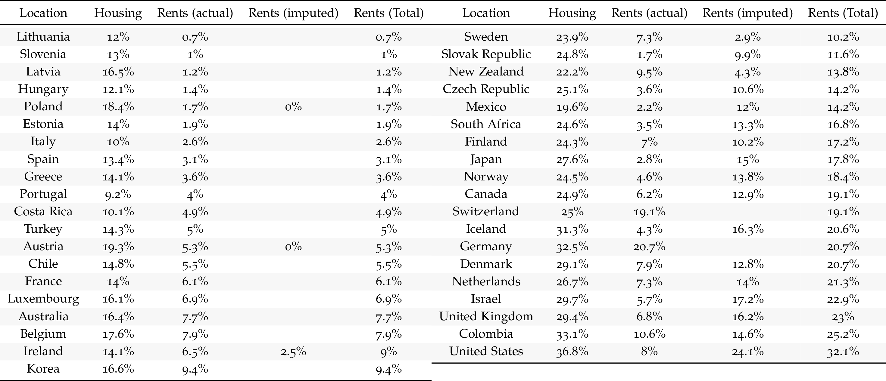
PRICES_CPI |>
  filter(MEASURE == "AL",
         SUBJECT %in% c("PWCP0410", "PWCP0420", "PWCP0400"),
         obsTime %in% c("2019")) |>
  left_join(tibble(SUBJECT = c("PWCP0410", "PWCP0420", "PWCP0400"),
                   Subject = c("Rents (actual)", "Rents (imputed)", "Housing")),
            by = "SUBJECT") |>
  left_join(PRICES_CPI_var$LOCATION, by = "LOCATION") |>
  select(Location, Subject, obsValue) |>
  mutate(obsValue = round(obsValue/10, 1)) |>
  spread(Subject, obsValue) |>
  mutate(`Rents (Total)` = `Rents (actual)` + ifelse(is.na(`Rents (imputed)`), 0, `Rents (imputed)`)) |>
  arrange(`Rents (Total)`) |>
  mutate(Flag = gsub(" ", "-", str_to_lower(Location)),
         Flag = paste0('<img src="../../icon/flag/vsmall/', Flag, '.png" alt="Flag">')) |>
  select(Flag, everything()) %>%
{if (is_html_output()) datatable(., filter = 'top', rownames = F, escape = F) else .}i_g("bib/oecd/PRICES_CPI_ex2.png")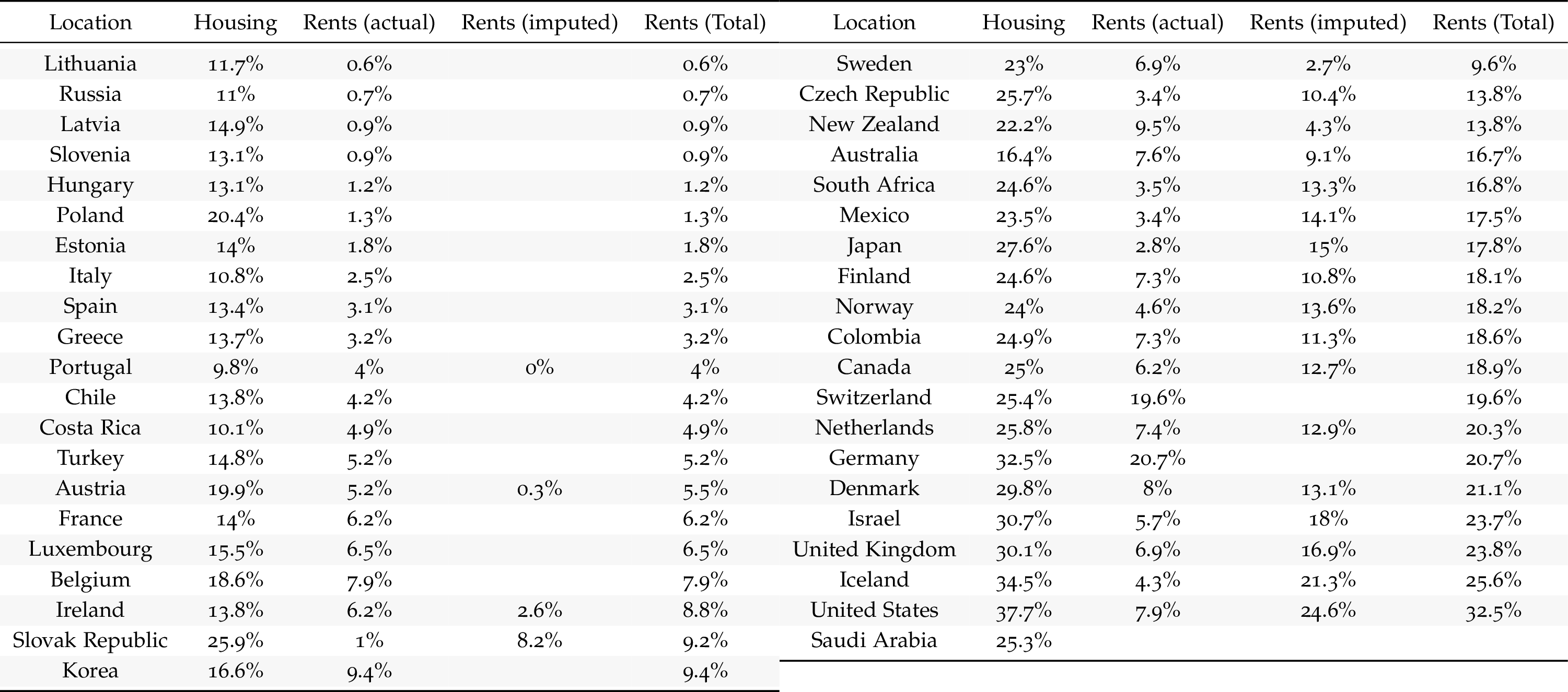
PRICES_CPI |>
  filter(LOCATION %in% c("FRA", "ITA", "DEU", "USA"),
         MEASURE == "AL",
         FREQUENCY == "A",
         SUBJECT == "PWCP0100") |>
  year_to_date() |>
  left_join(PRICES_CPI_var$LOCATION, by = "LOCATION") |>
  add_flag_color("Location") |>
  mutate(obsValue = obsValue/1000) |>
  ggplot() + geom_line(aes(x = date, y = obsValue, color = color)) +
  scale_color_identity() + add_4flags +
  theme_minimal() + xlab("") + ylab("Weights") +
  scale_x_date(breaks = seq(1960, 2100, 5) |> paste0("-01-01") |> as.Date(),
               labels = date_format("%Y")) +
  scale_y_continuous(breaks = 0.01*seq(0, 200, 1),
                     labels = scales::percent_format(accuracy = 1)) +
  theme(legend.position = c(0.7, 0.80),
        legend.title = element_blank())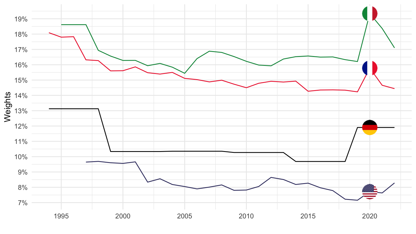
PRICES_CPI |>
  filter(LOCATION %in% c("FRA", "ITA", "DEU", "USA"),
         MEASURE == "AL",
         FREQUENCY == "A",
         SUBJECT == "PWCP0200") |>
  year_to_date() |>
  left_join(PRICES_CPI_var$LOCATION, by = "LOCATION") |>
  add_flag_color("Location") |>
  mutate(obsValue = obsValue/1000) |>
  ggplot() + geom_line(aes(x = date, y = obsValue, color = color)) +
  scale_color_identity() + add_4flags +
  theme_minimal() + xlab("") + ylab("Weights") +
  scale_x_date(breaks = seq(1960, 2100, 5) |> paste0("-01-01") |> as.Date(),
               labels = date_format("%Y")) +
  scale_y_continuous(breaks = 0.01*seq(0, 200, 1),
                     labels = scales::percent_format(accuracy = 1)) +
  theme(legend.position = c(0.7, 0.80),
        legend.title = element_blank())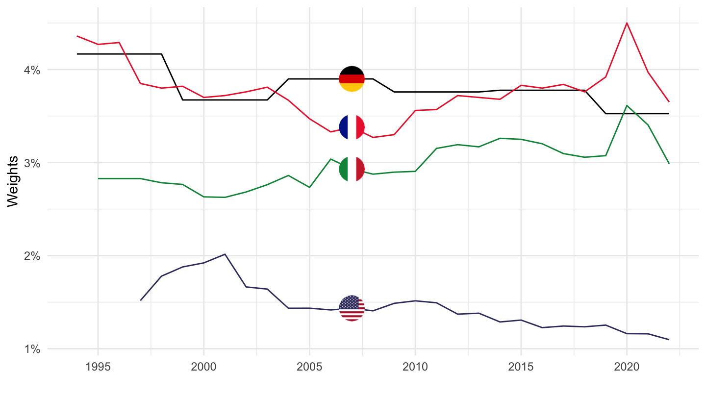
PRICES_CPI |>
  filter(LOCATION %in% c("FRA", "ITA", "DEU", "USA"),
         MEASURE == "AL",
         FREQUENCY == "A",
         SUBJECT == "PWCP0800") |>
  year_to_date() |>
  left_join(PRICES_CPI_var$LOCATION, by = "LOCATION") |>
  add_flag_color("Location") |>
  mutate(obsValue = obsValue/1000) |>
  ggplot() + geom_line(aes(x = date, y = obsValue, color = color)) +
  scale_color_identity() + add_4flags +
  theme_minimal() + xlab("") + ylab("Weights") +
  scale_x_date(breaks = seq(1960, 2100, 5) |> paste0("-01-01") |> as.Date(),
               labels = date_format("%Y")) +
  scale_y_continuous(breaks = 0.01*seq(0, 200, 1),
                     labels = scales::percent_format(accuracy = 1)) +
  theme(legend.position = c(0.7, 0.80),
        legend.title = element_blank())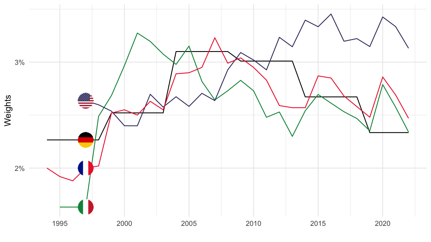
PRICES_CPI |>
  filter(LOCATION %in% c("FRA", "ITA", "DEU", "USA"),
         MEASURE == "AL",
         FREQUENCY == "A",
         SUBJECT == "PWCP0400") |>
  year_to_date() |>
  left_join(PRICES_CPI_var$LOCATION, by = "LOCATION") |>
  add_flag_color("Location") |>
  mutate(obsValue = obsValue/1000) |>
  ggplot() + geom_line(aes(x = date, y = obsValue, color = color)) +
  scale_color_identity() + add_4flags +
  theme_minimal() + xlab("") + ylab("CPI, Real Actual rentals for housing") +
  scale_x_date(breaks = seq(1960, 2100, 5) |> paste0("-01-01") |> as.Date(),
               labels = date_format("%Y")) +
  scale_y_continuous(breaks = 0.01*seq(0, 200, 1),
                     labels = scales::percent_format(accuracy = 1)) +
  theme(legend.position = c(0.7, 0.80),
        legend.title = element_blank())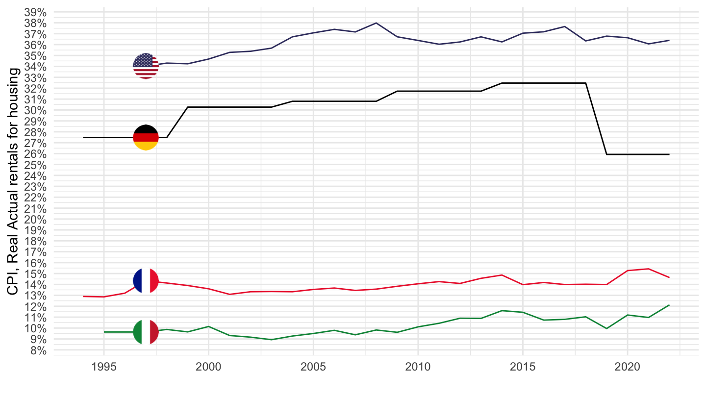
PRICES_CPI |>
  filter(LOCATION %in% c("FRA", "ITA", "DEU", "USA"),
         MEASURE == "AL",
         FREQUENCY == "A",
         SUBJECT == "PWCP0410") |>
  year_to_date() |>
  left_join(PRICES_CPI_var$LOCATION, by = "LOCATION") |>
  add_flag_color("Location") |>
  mutate(obsValue = obsValue/1000) |>
  ggplot() + geom_line(aes(x = date, y = obsValue, color = color)) +
  scale_color_identity() + add_4flags +
  theme_minimal() + xlab("") + ylab("CPI, Real Actual rentals for housing") +
  scale_x_date(breaks = seq(1960, 2100, 5) |> paste0("-01-01") |> as.Date(),
               labels = date_format("%Y")) +
  scale_y_continuous(breaks = 0.01*seq(0, 200, 1),
                     labels = scales::percent_format(accuracy = 1)) +
  theme(legend.position = c(0.7, 0.80),
        legend.title = element_blank())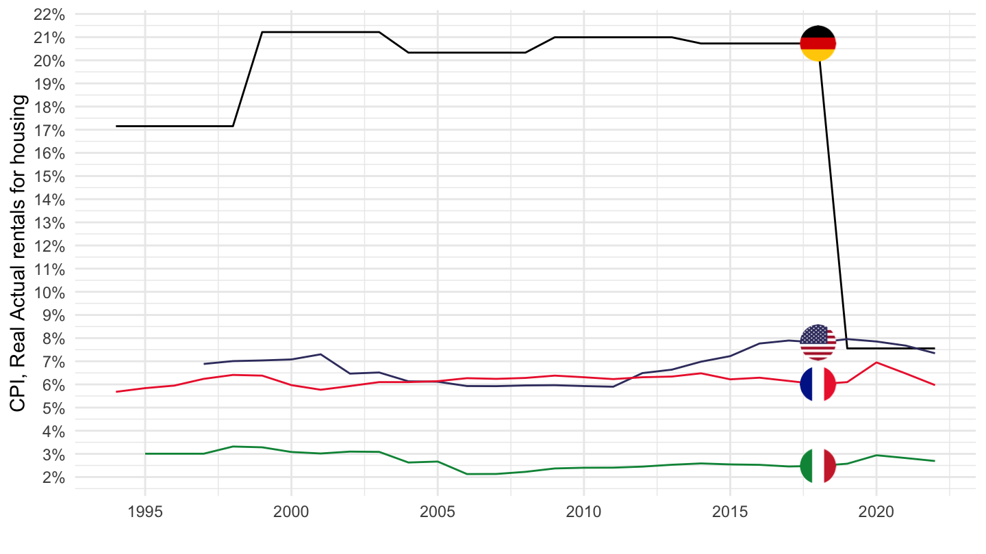
PRICES_CPI |>
  filter(LOCATION %in% c("FRA", "ITA", "DEU", "USA"),
         MEASURE == "AL",
         FREQUENCY == "A",
         SUBJECT == "PWCP0420") |>
  year_to_date() |>
  left_join(PRICES_CPI_var$LOCATION, by = "LOCATION") |>
  add_flag_color("Location") |>
  mutate(obsValue = obsValue/1000) |>
  ggplot() + geom_line(aes(x = date, y = obsValue, color = color)) +
  scale_color_identity() + add_4flags +
  theme_minimal() + xlab("") + ylab("CPI, Real Actual rentals for housing") +
  scale_x_date(breaks = seq(1960, 2100, 5) |> paste0("-01-01") |> as.Date(),
               labels = date_format("%Y")) +
  scale_y_continuous(breaks = 0.01*seq(0, 200, 1),
                     labels = scales::percent_format(accuracy = 1)) +
  theme(legend.position = c(0.7, 0.80),
        legend.title = element_blank())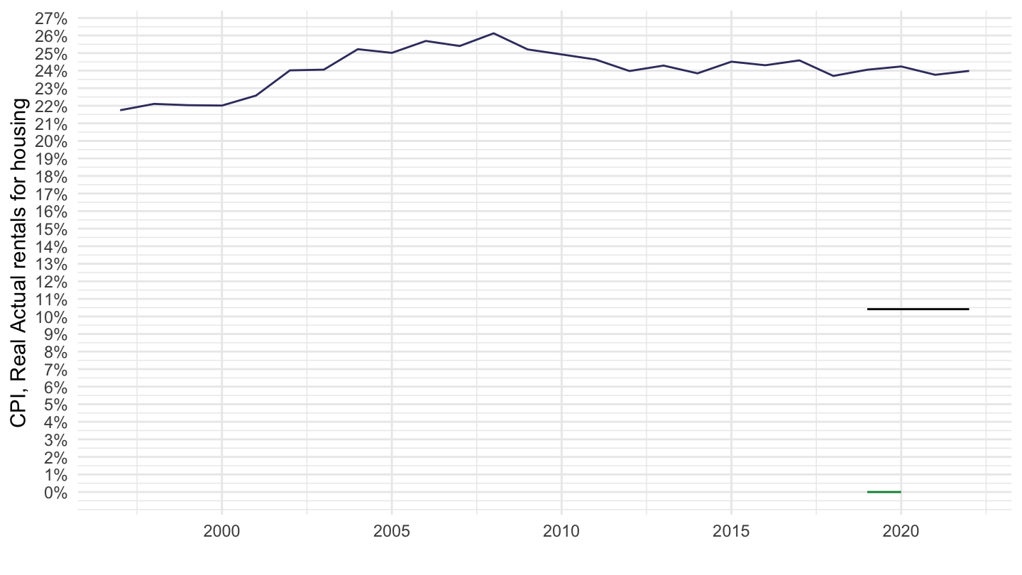
PRICES_CPI |>
  filter(LOCATION %in% c("FRA", "ITA", "DEU", "USA"),
         MEASURE == "AL",
         FREQUENCY == "A",
         SUBJECT == "PWCP0300") |>
  year_to_date() |>
  left_join(PRICES_CPI_var$LOCATION, by = "LOCATION") |>
  add_flag_color("Location") |>
  mutate(obsValue = obsValue/1000) |>
  ggplot() + geom_line(aes(x = date, y = obsValue, color = color)) +
  scale_color_identity() + add_4flags +
  theme_minimal() + xlab("") + ylab("Weights") +
  scale_x_date(breaks = seq(1960, 2100, 5) |> paste0("-01-01") |> as.Date(),
               labels = date_format("%Y")) +
  scale_y_continuous(breaks = 0.01*seq(0, 200, 1),
                     labels = scales::percent_format(accuracy = 1)) +
  theme(legend.position = c(0.7, 0.80),
        legend.title = element_blank())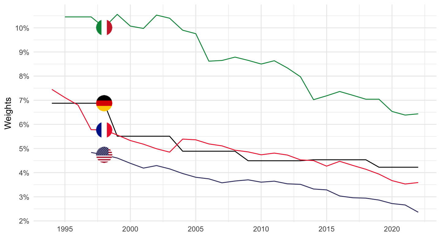
PRICES_CPI |>
  filter(LOCATION %in% c("FRA", "ITA", "DEU", "USA"),
         MEASURE == "AL",
         FREQUENCY == "A",
         SUBJECT == "PWCP0500") |>
  year_to_date() |>
  left_join(PRICES_CPI_var$LOCATION, by = "LOCATION") |>
  add_flag_color("Location") |>
  mutate(obsValue = obsValue/1000) |>
  ggplot() + geom_line(aes(x = date, y = obsValue, color = color)) +
  scale_color_identity() + add_4flags +
  theme_minimal() + xlab("") + ylab("Weights") +
  scale_x_date(breaks = seq(1960, 2100, 5) |> paste0("-01-01") |> as.Date(),
               labels = date_format("%Y")) +
  scale_y_continuous(breaks = 0.01*seq(0, 200, 1),
                     labels = scales::percent_format(accuracy = 1)) +
  theme(legend.position = c(0.7, 0.80),
        legend.title = element_blank())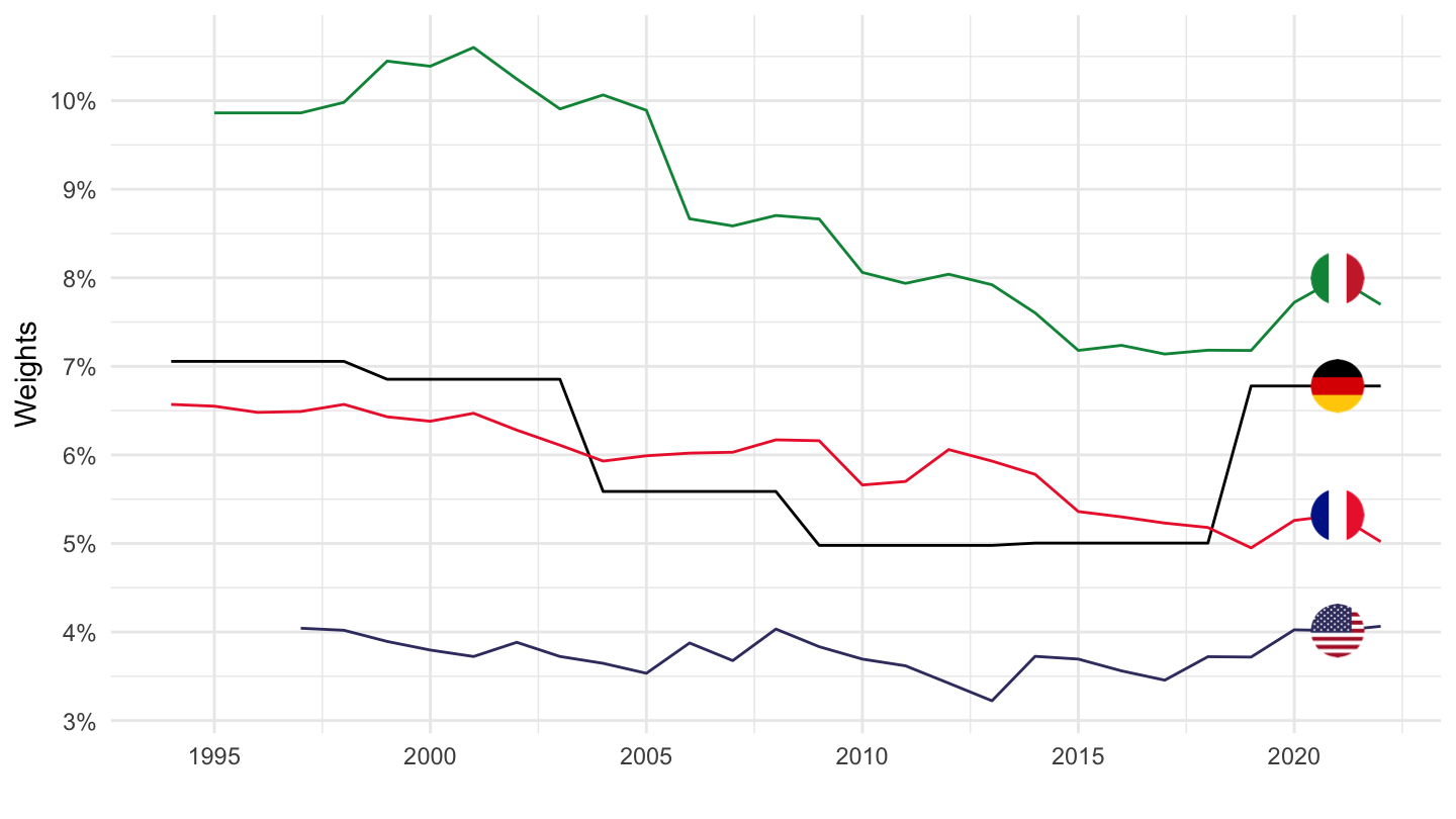
PRICES_CPI |>
  filter(LOCATION %in% c("FRA", "ITA", "DEU", "USA"),
         MEASURE == "AL",
         FREQUENCY == "A",
         SUBJECT == "PWCP0600") |>
  year_to_date() |>
  left_join(PRICES_CPI_var$LOCATION, by = "LOCATION") |>
  add_flag_color("Location") |>
  mutate(obsValue = obsValue/1000) |>
  ggplot() + geom_line(aes(x = date, y = obsValue, color = color)) +
  scale_color_identity() + add_4flags +
  theme_minimal() + xlab("") + ylab("Weights") +
  scale_x_date(breaks = seq(1960, 2100, 5) |> paste0("-01-01") |> as.Date(),
               labels = date_format("%Y")) +
  scale_y_continuous(breaks = 0.01*seq(0, 200, 1),
                     labels = scales::percent_format(accuracy = 1)) +
  theme(legend.position = c(0.7, 0.80),
        legend.title = element_blank())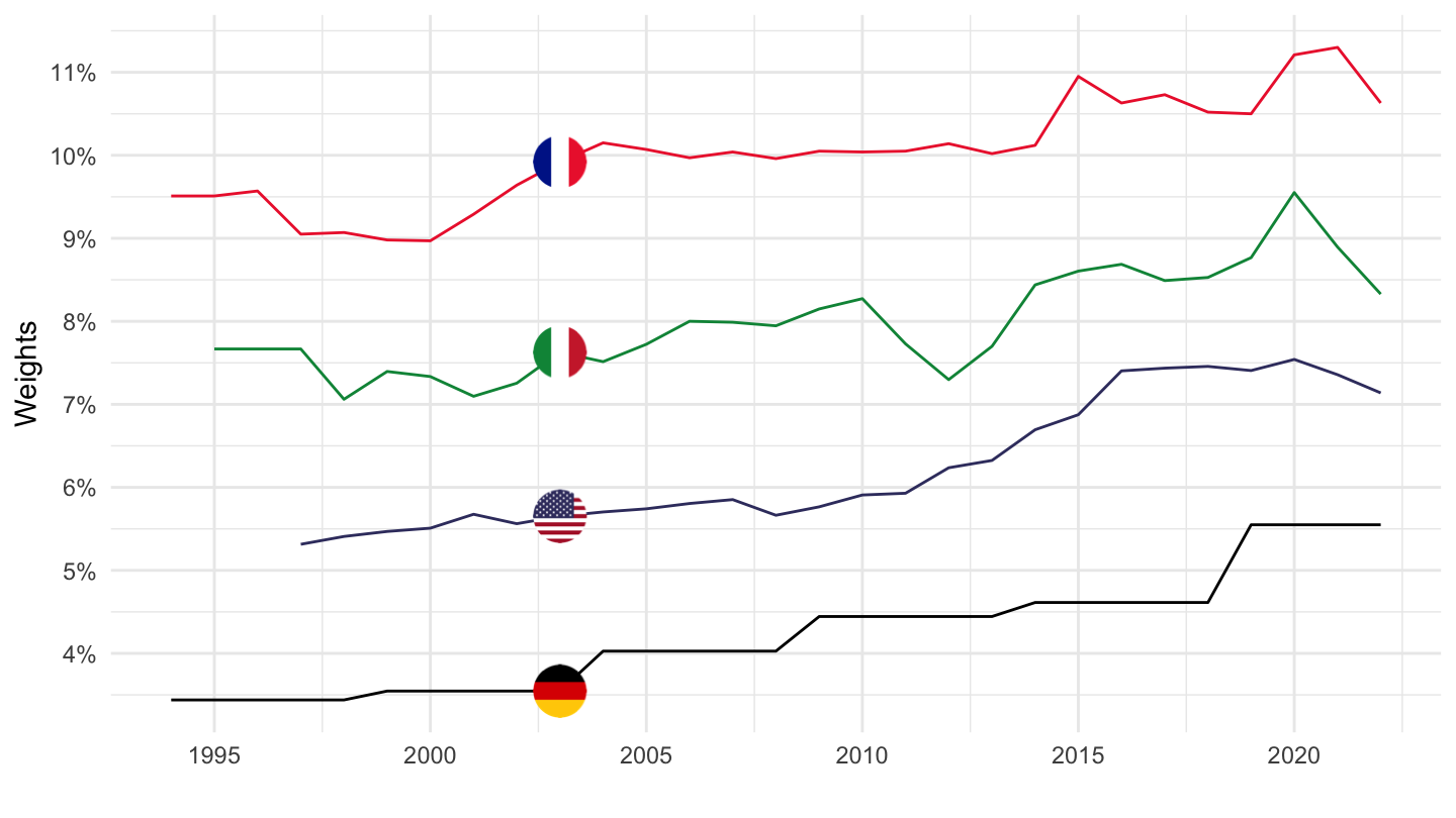
PRICES_CPI |>
  filter(LOCATION %in% c("FRA", "ITA", "DEU", "USA"),
         MEASURE == "AL",
         FREQUENCY == "A",
         SUBJECT == "PWCP0700") |>
  year_to_date() |>
  left_join(PRICES_CPI_var$LOCATION, by = "LOCATION") |>
  add_flag_color("Location") |>
  mutate(obsValue = obsValue/1000) |>
  ggplot() + geom_line(aes(x = date, y = obsValue, color = color)) +
  scale_color_identity() + add_4flags +
  theme_minimal() + xlab("") + ylab("Weights") +
  scale_x_date(breaks = seq(1960, 2100, 5) |> paste0("-01-01") |> as.Date(),
               labels = date_format("%Y")) +
  scale_y_continuous(breaks = 0.01*seq(0, 200, 1),
                     labels = scales::percent_format(accuracy = 1)) +
  theme(legend.position = c(0.7, 0.80),
        legend.title = element_blank())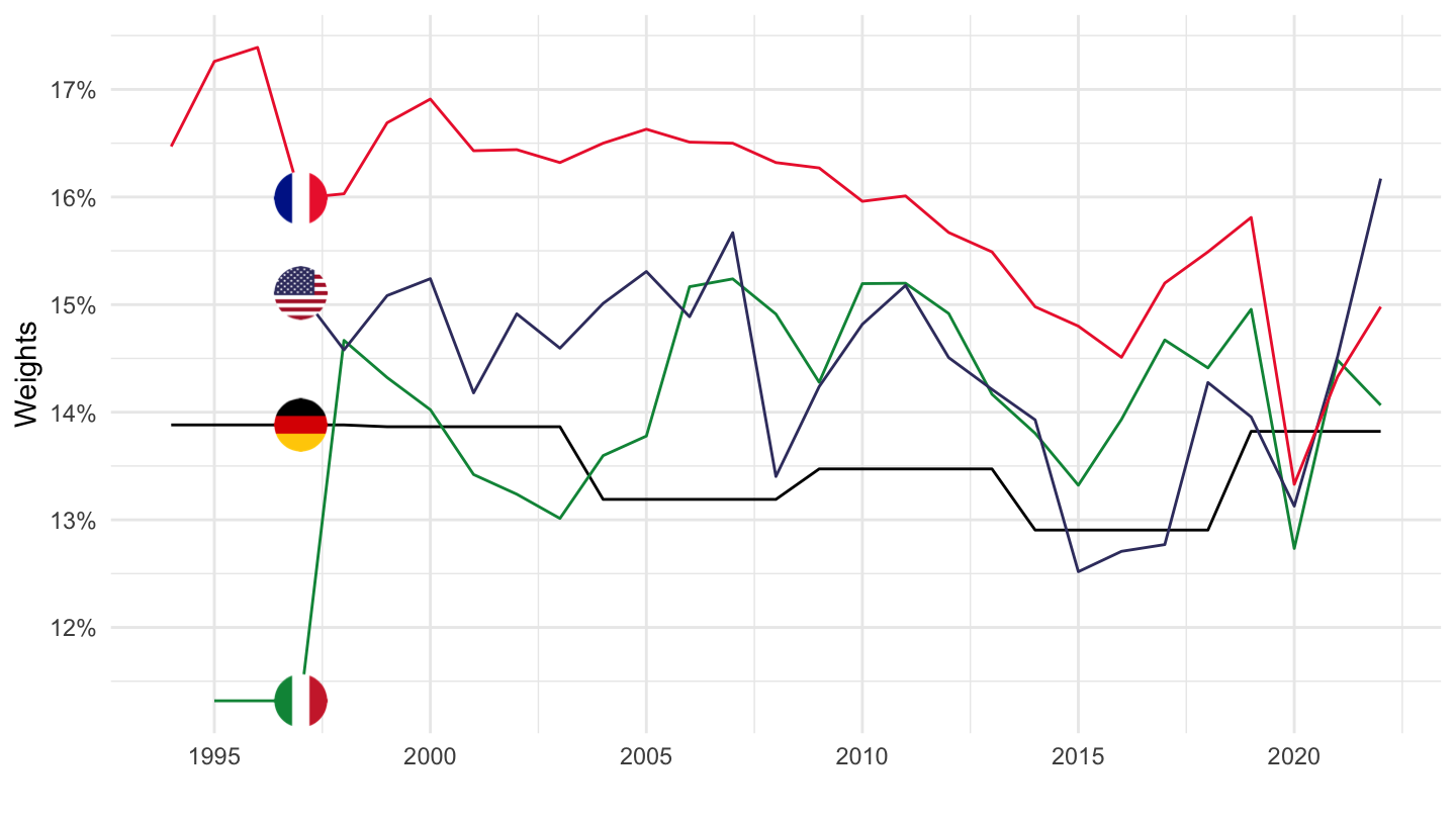
PRICES_CPI |>
  filter(LOCATION %in% c("FRA", "ITA", "DEU", "USA"),
         MEASURE == "AL",
         FREQUENCY == "A",
         SUBJECT == "PWCP0900") |>
  year_to_date() |>
  left_join(PRICES_CPI_var$LOCATION, by = "LOCATION") |>
  add_flag_color("Location") |>
  mutate(obsValue = obsValue/1000) |>
  ggplot() + geom_line(aes(x = date, y = obsValue, color = color)) +
  scale_color_identity() + add_4flags +
  theme_minimal() + xlab("") + ylab("Weights") +
  scale_x_date(breaks = seq(1960, 2100, 5) |> paste0("-01-01") |> as.Date(),
               labels = date_format("%Y")) +
  scale_y_continuous(breaks = 0.01*seq(0, 200, 1),
                     labels = scales::percent_format(accuracy = 1)) +
  theme(legend.position = c(0.7, 0.80),
        legend.title = element_blank())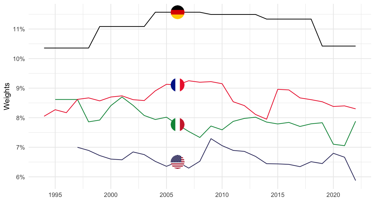
PRICES_CPI |>
  filter(LOCATION %in% c("FRA", "ITA", "DEU", "USA"),
         MEASURE == "AL",
         FREQUENCY == "A",
         SUBJECT == "PWCP1000") |>
  year_to_date() |>
  left_join(PRICES_CPI_var$LOCATION, by = "LOCATION") |>
  add_flag_color("Location") |>
  mutate(obsValue = obsValue/1000) |>
  ggplot() + geom_line(aes(x = date, y = obsValue, color = color)) +
  scale_color_identity() + add_4flags +
  theme_minimal() + xlab("") + ylab("Weights") +
  scale_x_date(breaks = seq(1960, 2100, 5) |> paste0("-01-01") |> as.Date(),
               labels = date_format("%Y")) +
  scale_y_continuous(breaks = 0.01*seq(0, 200, 1),
                     labels = scales::percent_format(accuracy = 1)) +
  theme(legend.position = c(0.7, 0.80),
        legend.title = element_blank())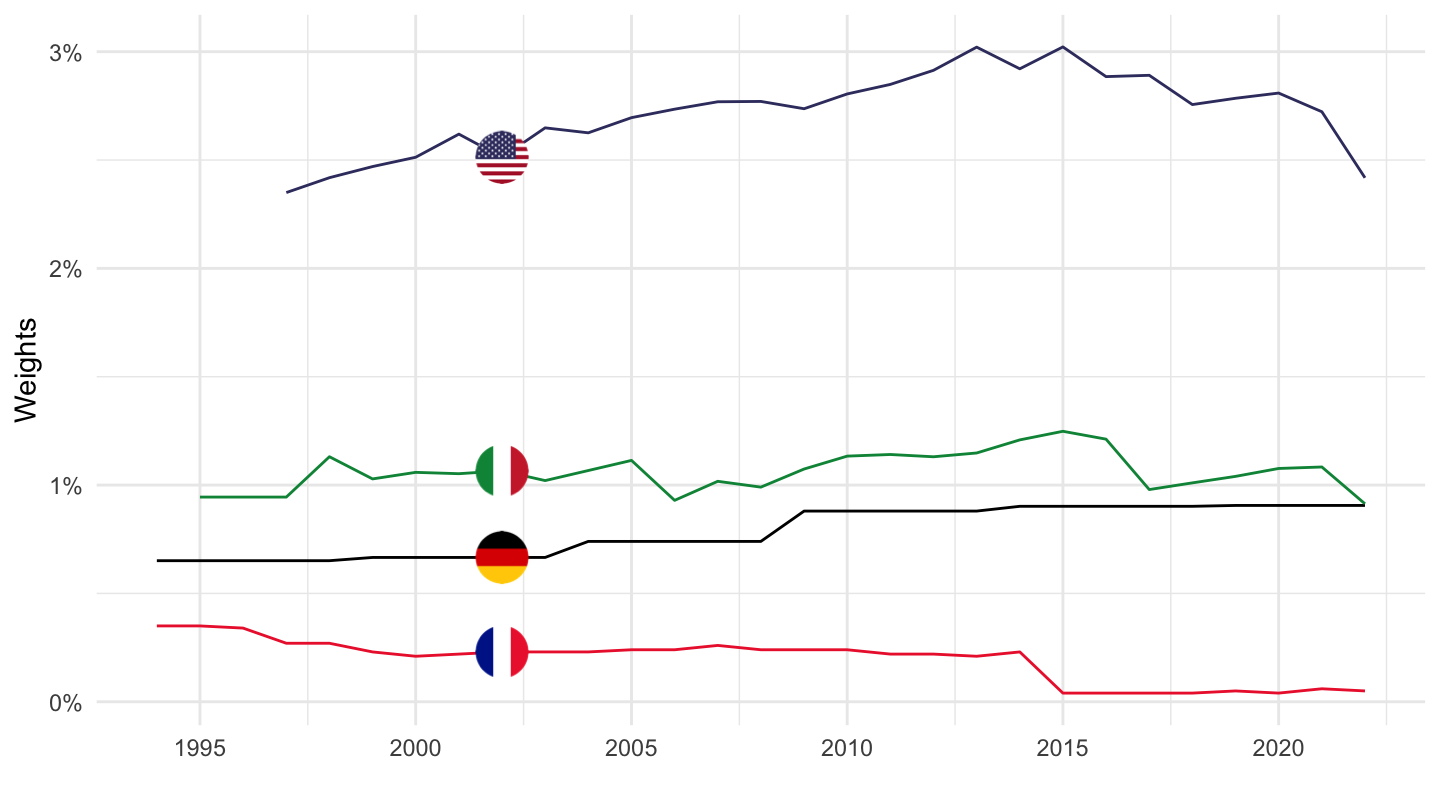
PRICES_CPI |>
  filter(LOCATION %in% c("FRA", "ITA", "DEU", "USA"),
         MEASURE == "AL",
         FREQUENCY == "A",
         SUBJECT == "PWCP1100") |>
  year_to_date() |>
  left_join(PRICES_CPI_var$LOCATION, by = "LOCATION") |>
  add_flag_color("Location") |>
  mutate(obsValue = obsValue/1000) |>
  ggplot() + geom_line(aes(x = date, y = obsValue, color = color)) +
  scale_color_identity() + add_4flags +
  theme_minimal() + xlab("") + ylab("Weights") +
  scale_x_date(breaks = seq(1960, 2100, 5) |> paste0("-01-01") |> as.Date(),
               labels = date_format("%Y")) +
  scale_y_continuous(breaks = 0.01*seq(0, 200, 1),
                     labels = scales::percent_format(accuracy = 1)) +
  theme(legend.position = c(0.7, 0.80),
        legend.title = element_blank())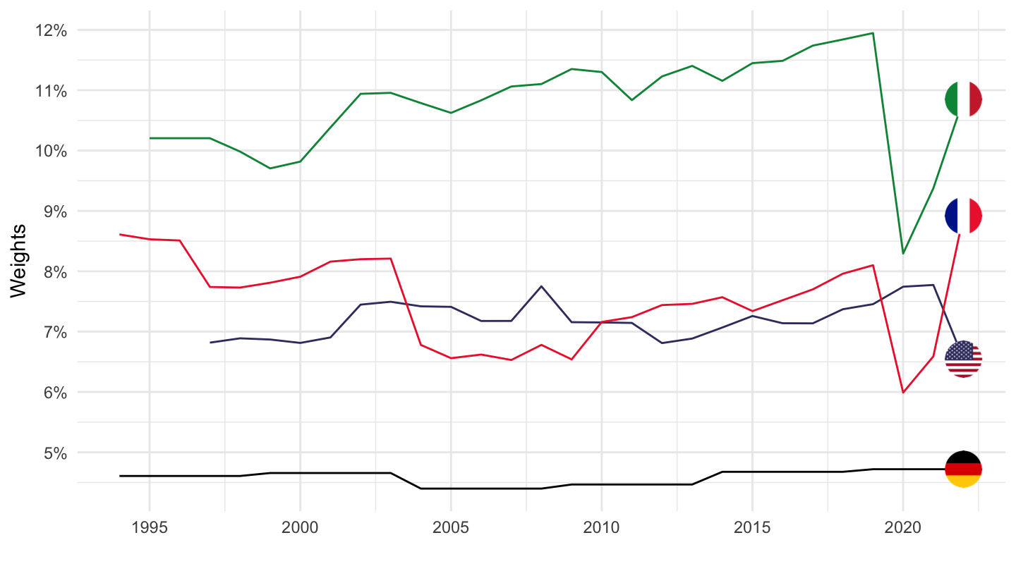
PRICES_CPI |>
  filter(LOCATION %in% c("FRA", "ITA", "DEU", "USA"),
         MEASURE == "AL",
         FREQUENCY == "A",
         SUBJECT == "PWCP1200") |>
  year_to_date() |>
  left_join(PRICES_CPI_var$LOCATION, by = "LOCATION") |>
  add_flag_color("Location") |>
  mutate(obsValue = obsValue/1000) |>
  ggplot() + geom_line(aes(x = date, y = obsValue, color = color)) +
  scale_color_identity() + add_4flags +
  theme_minimal() + xlab("") + ylab("Weights") +
  scale_x_date(breaks = seq(1960, 2100, 5) |> paste0("-01-01") |> as.Date(),
               labels = date_format("%Y")) +
  scale_y_continuous(breaks = 0.01*seq(0, 200, 1),
                     labels = scales::percent_format(accuracy = 1)) +
  theme(legend.position = c(0.7, 0.80),
        legend.title = element_blank())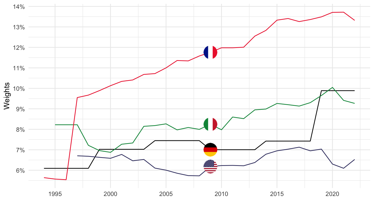
PRICES_CPI |>
  filter(LOCATION %in% c("ISR"),
         MEASURE == "AL",
         FREQUENCY == "A",
         obsTime %in% c("1994", "1999", "2009", "2019")) |>
  left_join(PRICES_CPI_var$SUBJECT, by = "SUBJECT") |>
  select(SUBJECT, Subject, obsTime, obsValue) |>
  spread(obsTime, obsValue) %>%
{if (is_html_output()) datatable(., filter = 'top', rownames = F) else .}PRICES_CPI |>
filter(LOCATION %in% c("CHE"),
MEASURE == "AL",
FREQUENCY == "A",
obsTime %in% c("1994", "1999", "2009", "2019")) |>
left_join(PRICES_CPI_var$SUBJECT, by = "SUBJECT") |>
select(SUBJECT, Subject, obsTime, obsValue) |>
spread(obsTime, obsValue) %>%
{if (is_html_output()) datatable(., filter = 'top', rownames = F) else .}PRICES_CPI |>
filter(LOCATION %in% c("FRA"),
MEASURE == "AL",
FREQUENCY == "A",
obsTime %in% c("1994", "1999", "2009", "2019")) |>
left_join(PRICES_CPI_var$SUBJECT, by = "SUBJECT") |>
select(SUBJECT, Subject, obsTime, obsValue) |>
spread(obsTime, obsValue) %>%
{if (is_html_output()) datatable(., filter = 'top', rownames = F) else .}PRICES_CPI |>
filter(LOCATION %in% c("AUS"),
MEASURE == "AL",
FREQUENCY == "A",
obsTime %in% c("1994", "1999", "2009", "2019")) |>
left_join(PRICES_CPI_var$SUBJECT, by = "SUBJECT") |>
select(SUBJECT, Subject, obsTime, obsValue) |>
spread(obsTime, obsValue) %>%
{if (is_html_output()) datatable(., filter = 'top', rownames = F) else .}PRICES_CPI |>
filter(LOCATION %in% c("USA"),
MEASURE == "AL",
FREQUENCY == "A",
obsTime %in% c("1994", "1999", "2009", "2019")) |>
left_join(PRICES_CPI_var$SUBJECT, by = "SUBJECT") |>
select(SUBJECT, Subject, obsTime, obsValue) |>
spread(obsTime, obsValue) %>%
{if (is_html_output()) datatable(., filter = 'top', rownames = F) else .}PRICES_CPI |>
filter(LOCATION %in% c("ISR"),
FREQUENCY == "Q",
MEASURE == "IXOB") |>
left_join(PRICES_CPI_var$SUBJECT, by = "SUBJECT") |>
group_by(SUBJECT, Subject) |>
summarise(Nobs = n(),
min = min(obsTime),
max = max(obsTime)) %>%
{if (is_html_output()) datatable(., filter = 'top', rownames = F) else .}PRICES_CPI |>
filter(LOCATION %in% c("CHE"),
FREQUENCY == "Q",
MEASURE == "IXOB") |>
left_join(PRICES_CPI_var$SUBJECT, by = "SUBJECT") |>
group_by(SUBJECT, Subject) |>
summarise(Nobs = n(),
min = min(obsTime),
max = max(obsTime)) %>%
{if (is_html_output()) datatable(., filter = 'top', rownames = F) else .}PRICES_CPI |>
filter(LOCATION %in% c("FRA"),
FREQUENCY == "Q",
MEASURE == "IXOB") |>
left_join(PRICES_CPI_var$SUBJECT, by = "SUBJECT") |>
group_by(SUBJECT, Subject) |>
summarise(Nobs = n(),
min = min(obsTime),
max = max(obsTime)) %>%
{if (is_html_output()) datatable(., filter = 'top', rownames = F) else .}PRICES_CPI |>
filter(LOCATION %in% c("USA"),
FREQUENCY == "Q",
MEASURE == "IXOB") |>
left_join(PRICES_CPI_var$SUBJECT, by = "SUBJECT") |>
group_by(SUBJECT, Subject) |>
summarise(Nobs = n(),
min = min(obsTime),
max = max(obsTime)) %>%
{if (is_html_output()) datatable(., filter = 'top', rownames = F) else .}PRICES_CPI |>
filter(SUBJECT %in% c("CP040100", "CPALTT01"),
FREQUENCY == "Q",
MEASURE == "GY",
obsTime == "2019-Q4") |>
quarter_to_date() |>
left_join(PRICES_CPI_var$LOCATION, by = "LOCATION") |>
select(LOCATION, Location, SUBJECT, obsValue) |>
mutate(obsValue = round(obsValue, 1)) |>
spread(SUBJECT, obsValue) |>
mutate(Flag = gsub(" ", "-", str_to_lower(Location)),
Flag = paste0('<img src="../../icon/flag/vsmall/', Flag, '.png" alt="Flag">')) |>
select(Flag, everything()) %>%
{if (is_html_output()) datatable(., filter = 'top', rownames = F, escape = F) else .}PRICES_CPI |>
filter(LOCATION %in% c("ISL"),
SUBJECT %in% c("CP040100", "CPALTT01"),
FREQUENCY == "Q",
MEASURE == "GY") |>
quarter_to_date() |>
select(SUBJECT, date, LOCATION, obsValue) |>
spread(SUBJECT, obsValue) |>
filter(!is.na(CP040100)) |>
mutate(rents_real = CP040100-CPALTT01) |>
select(date, LOCATION, CPALTT01, CP040100) |>
gather(variable, value, - date, -LOCATION) |>
mutate(Variable = case_when(variable == "CP040100" ~ "Rents",
variable == "CPALTT01" ~ "CPI")) |>
left_join(PRICES_CPI_var$LOCATION, by = "LOCATION") |>
ggplot() + theme_minimal() + xlab("") + ylab("CPI") +
geom_line(aes(x = date, y = value/100, color = Variable, linetype = Variable)) +
scale_x_date(breaks = seq(1960, 2100, 2) |> paste0("-01-01") |> as.Date(),
labels = date_format("%Y")) +
scale_y_continuous(breaks = 0.01*seq(-100, 200, 5),
labels = percent_format(acc = 1)) +
scale_color_manual(values = viridis(3)[1:2]) +
theme(legend.position = c(0.7, 0.30),
legend.title = element_blank())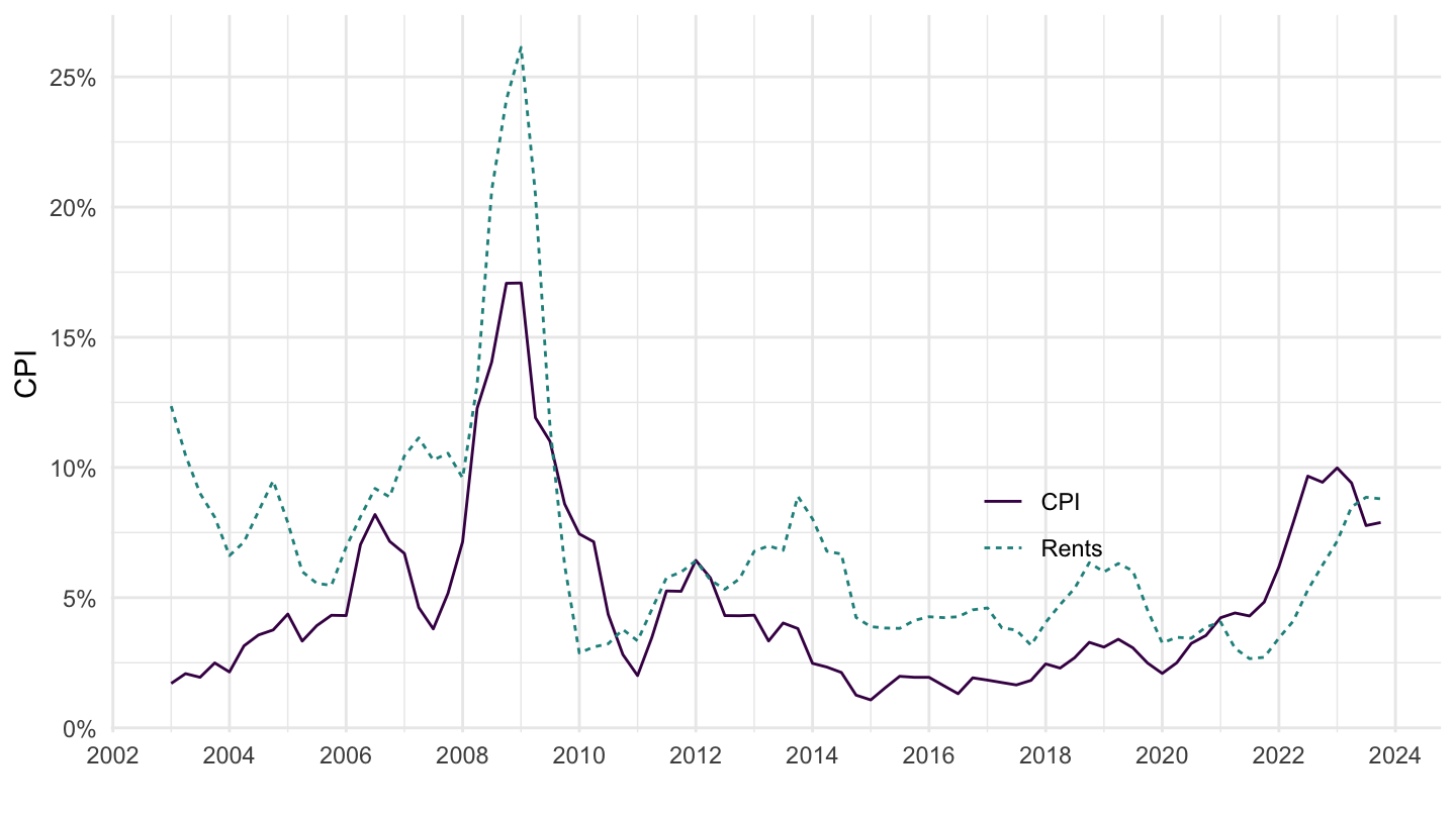
PRICES_CPI |>
  filter(LOCATION %in% c("JPN"),
         SUBJECT %in% c("CP040100", "CPALTT01"),
         FREQUENCY == "Q",
         MEASURE == "GY") |>
  quarter_to_date() |>
  select(SUBJECT, date, LOCATION, obsValue) |>
  spread(SUBJECT, obsValue) |>
  filter(!is.na(CP040100)) |>
  mutate(rents_real = CP040100-CPALTT01) |>
  select(date, LOCATION, CPALTT01, CP040100) |>
  gather(variable, value, - date, -LOCATION) |>
  mutate(Variable = case_when(variable == "CP040100" ~ "Rents",
                              variable == "CPALTT01" ~ "CPI")) |>
  left_join(PRICES_CPI_var$LOCATION, by = "LOCATION") |>
  ggplot() + theme_minimal() + xlab("") + ylab("CPI") +
  geom_line(aes(x = date, y = value/100, color = Variable, linetype = Variable)) +
  scale_x_date(breaks = seq(1960, 2100, 5) |> paste0("-01-01") |> as.Date(),
               labels = date_format("%Y")) +
  scale_y_continuous(breaks = 0.01*seq(-100, 200, 5),
                     labels = percent_format(acc = 1)) +
  scale_color_manual(values = viridis(3)[1:2]) +
  theme(legend.position = c(0.7, 0.30),
        legend.title = element_blank())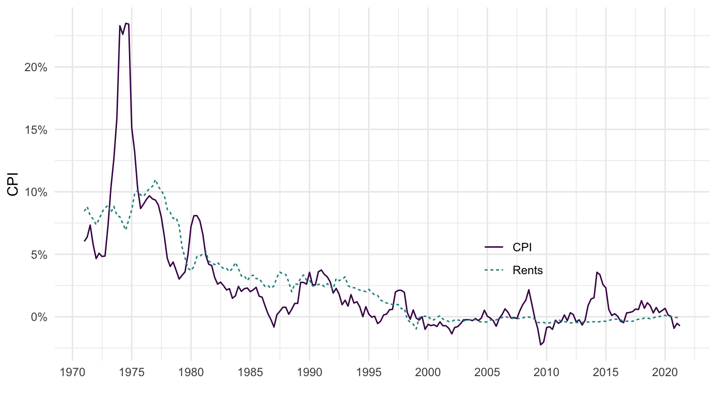
PRICES_CPI |>
  filter(LOCATION %in% c("JPN"),
         SUBJECT %in% c("CP040100", "CPALTT01"),
         FREQUENCY == "Q",
         MEASURE == "GY") |>
  quarter_to_date() |>
  select(SUBJECT, date, LOCATION, obsValue) |>
  spread(SUBJECT, obsValue) |>
  filter(!is.na(CP040100),
         date >= as.Date("1985-01-01")) |>
  mutate(rents_real = CP040100-CPALTT01) |>
  select(date, LOCATION, CPALTT01, CP040100) |>
  gather(variable, value, - date, -LOCATION) |>
  mutate(Variable = case_when(variable == "CP040100" ~ "Rents",
                              variable == "CPALTT01" ~ "CPI")) |>
  left_join(PRICES_CPI_var$LOCATION, by = "LOCATION") |>
  ggplot() + theme_minimal() + xlab("") + ylab("Inflation") +
  geom_line(aes(x = date, y = value/100, color = Variable)) +
  scale_x_date(breaks = seq(1960, 2100, 5) |> paste0("-01-01") |> as.Date(),
               labels = date_format("%Y")) +
  scale_y_continuous(breaks = 0.01*seq(-100, 200, 1),
                     labels = percent_format(acc = 1)) +
  scale_color_manual(values = viridis(3)[1:2]) +
  theme(legend.position = c(0.9, 0.9),
        legend.title = element_blank())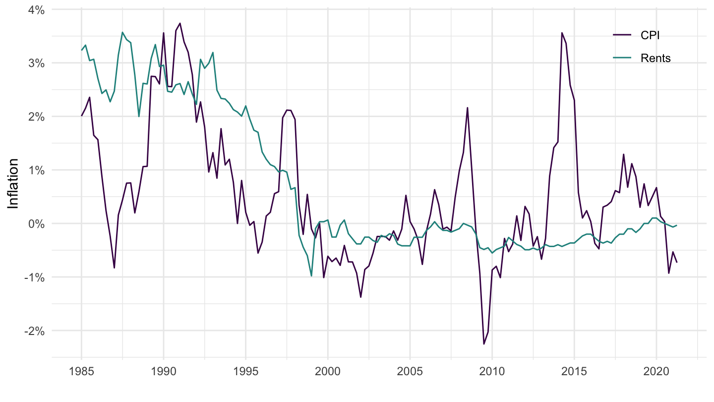
PRICES_CPI |>
  filter(LOCATION %in% c("ISR"),
         SUBJECT %in% c("CP040100", "CPALTT01"),
         FREQUENCY == "Q",
         MEASURE == "GY") |>
  quarter_to_date() |>
  select(SUBJECT, date, LOCATION, obsValue) |>
  spread(SUBJECT, obsValue) |>
  filter(!is.na(CP040100),
         date >= as.Date("1993-01-01")) |>
  mutate(rents_real = CP040100-CPALTT01) |>
  select(date, LOCATION, CPALTT01, CP040100) |>
  gather(variable, value, - date, -LOCATION) |>
  mutate(Variable = case_when(variable == "CP040100" ~ "Rents",
                              variable == "CPALTT01" ~ "CPI")) |>
  left_join(PRICES_CPI_var$LOCATION, by = "LOCATION") |>
  ggplot() + theme_minimal() + xlab("") + ylab("Inflation") +
  geom_line(aes(x = date, y = value/100, color = Variable)) +
  scale_x_date(breaks = seq(1960, 2100, 5) |> paste0("-01-01") |> as.Date(),
               labels = date_format("%Y")) +
  scale_y_continuous(breaks = 0.01*seq(-100, 200, 1),
                     labels = percent_format(acc = 1)) +
  scale_color_manual(values = viridis(3)[1:2]) +
  theme(legend.position = c(0.9, 0.9),
        legend.title = element_blank())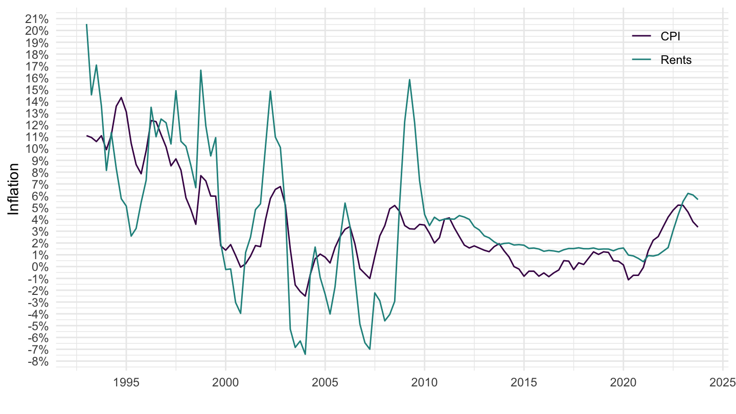
PRICES_CPI |>
  filter(LOCATION %in% c("GBR"),
         SUBJECT %in% c("CP040100", "CPALTT01"),
         FREQUENCY == "Q",
         MEASURE == "GY") |>
  quarter_to_date() |>
  select(SUBJECT, date, LOCATION, obsValue) |>
  spread(SUBJECT, obsValue) |>
  filter(!is.na(CP040100)) |>
  mutate(rents_real = CP040100-CPALTT01) |>
  select(date, LOCATION, CPALTT01, CP040100) |>
  gather(variable, value, - date, -LOCATION) |>
  mutate(Variable = case_when(variable == "CP040100" ~ "Rents",
                              variable == "CPALTT01" ~ "CPI")) |>
  left_join(PRICES_CPI_var$LOCATION, by = "LOCATION") |>
  ggplot() + theme_minimal() + xlab("") + ylab("Inflation") +
  geom_line(aes(x = date, y = value/100, color = Variable)) +
  scale_x_date(breaks = seq(1960, 2100, 5) |> paste0("-01-01") |> as.Date(),
               labels = date_format("%Y")) +
  scale_y_continuous(breaks = 0.01*seq(-100, 200, 1),
                     labels = percent_format(acc = 1)) +
  scale_color_manual(values = viridis(3)[1:2]) +
  theme(legend.position = c(0.9, 0.9),
        legend.title = element_blank())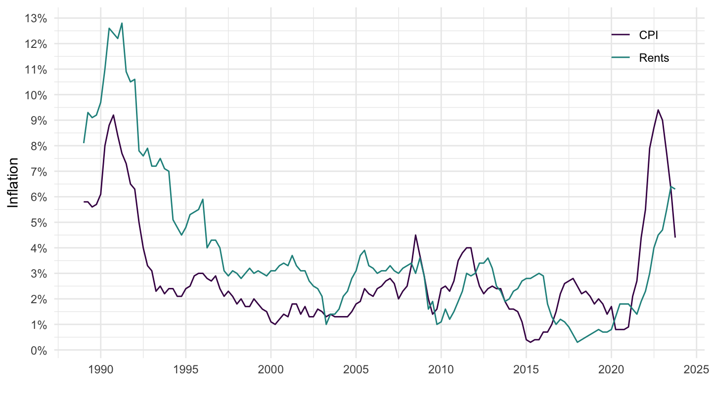
PRICES_CPI |>
  filter(LOCATION %in% c("GBR"),
         SUBJECT %in% c("CP040100", "CPALTT01"),
         FREQUENCY == "Q",
         MEASURE == "GY") |>
  quarter_to_date() |>
  select(SUBJECT, date, LOCATION, obsValue) |>
  spread(SUBJECT, obsValue) |>
  filter(!is.na(CP040100),
         date >= as.Date("1993-01-01")) |>
  mutate(rents_real = CP040100-CPALTT01) |>
  select(date, LOCATION, CPALTT01, CP040100) |>
  gather(variable, value, - date, -LOCATION) |>
  mutate(Variable = case_when(variable == "CP040100" ~ "Rents",
                              variable == "CPALTT01" ~ "CPI")) |>
  left_join(PRICES_CPI_var$LOCATION, by = "LOCATION") |>
  ggplot() + theme_minimal() + xlab("") + ylab("Inflation") +
  geom_line(aes(x = date, y = value/100, color = Variable)) +
  scale_x_date(breaks = seq(1960, 2100, 5) |> paste0("-01-01") |> as.Date(),
               labels = date_format("%Y")) +
  scale_y_continuous(breaks = 0.01*seq(-100, 200, 1),
                     labels = percent_format(acc = 1)) +
  scale_color_manual(values = viridis(3)[1:2]) +
  theme(legend.position = c(0.9, 0.9),
        legend.title = element_blank())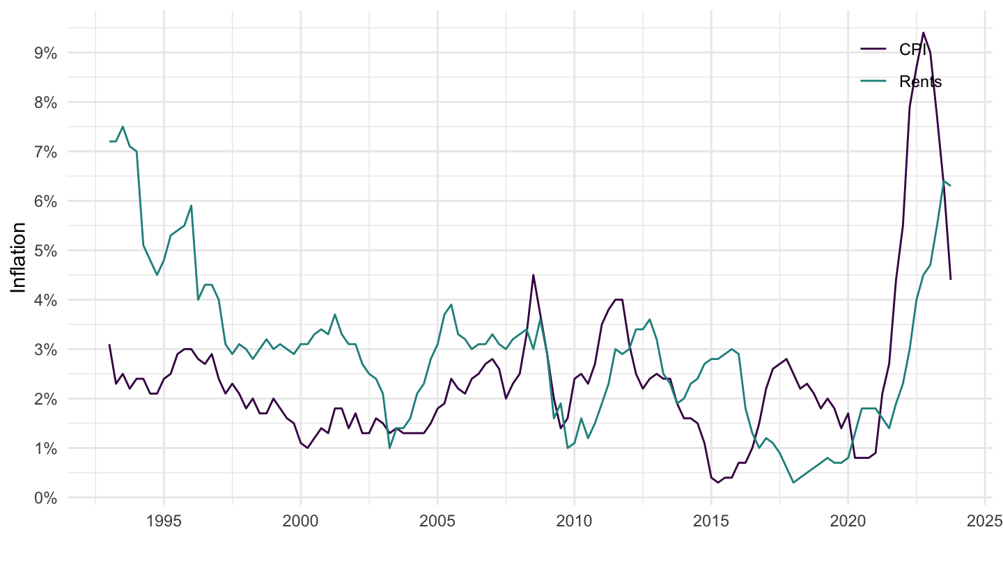
PRICES_CPI |>
  filter(LOCATION %in% c("GBR"),
         SUBJECT %in% c("CP040100", "CPALTT01"),
         FREQUENCY == "Q",
         MEASURE == "GY") |>
  quarter_to_date() |>
  select(SUBJECT, date, LOCATION, obsValue) |>
  spread(SUBJECT, obsValue) |>
  filter(!is.na(CP040100),
         date >= as.Date("2010-01-01")) |>
  mutate(rents_real = CP040100-CPALTT01) |>
  select(date, LOCATION, CPALTT01, CP040100) |>
  gather(variable, value, - date, -LOCATION) |>
  mutate(Variable = case_when(variable == "CP040100" ~ "Rents",
                              variable == "CPALTT01" ~ "CPI")) |>
  left_join(PRICES_CPI_var$LOCATION, by = "LOCATION") |>
  ggplot() + theme_minimal() + xlab("") + ylab("Inflation") +
  geom_line(aes(x = date, y = value/100, color = Variable)) +
  scale_x_date(breaks = seq(1960, 2100, 1) |> paste0("-01-01") |> as.Date(),
               labels = date_format("%Y")) +
  scale_y_continuous(breaks = 0.01*seq(-100, 200, 1),
                     labels = percent_format(acc = 1)) +
  scale_color_manual(values = viridis(3)[1:2]) +
  theme(legend.position = c(0.9, 0.9),
        legend.title = element_blank())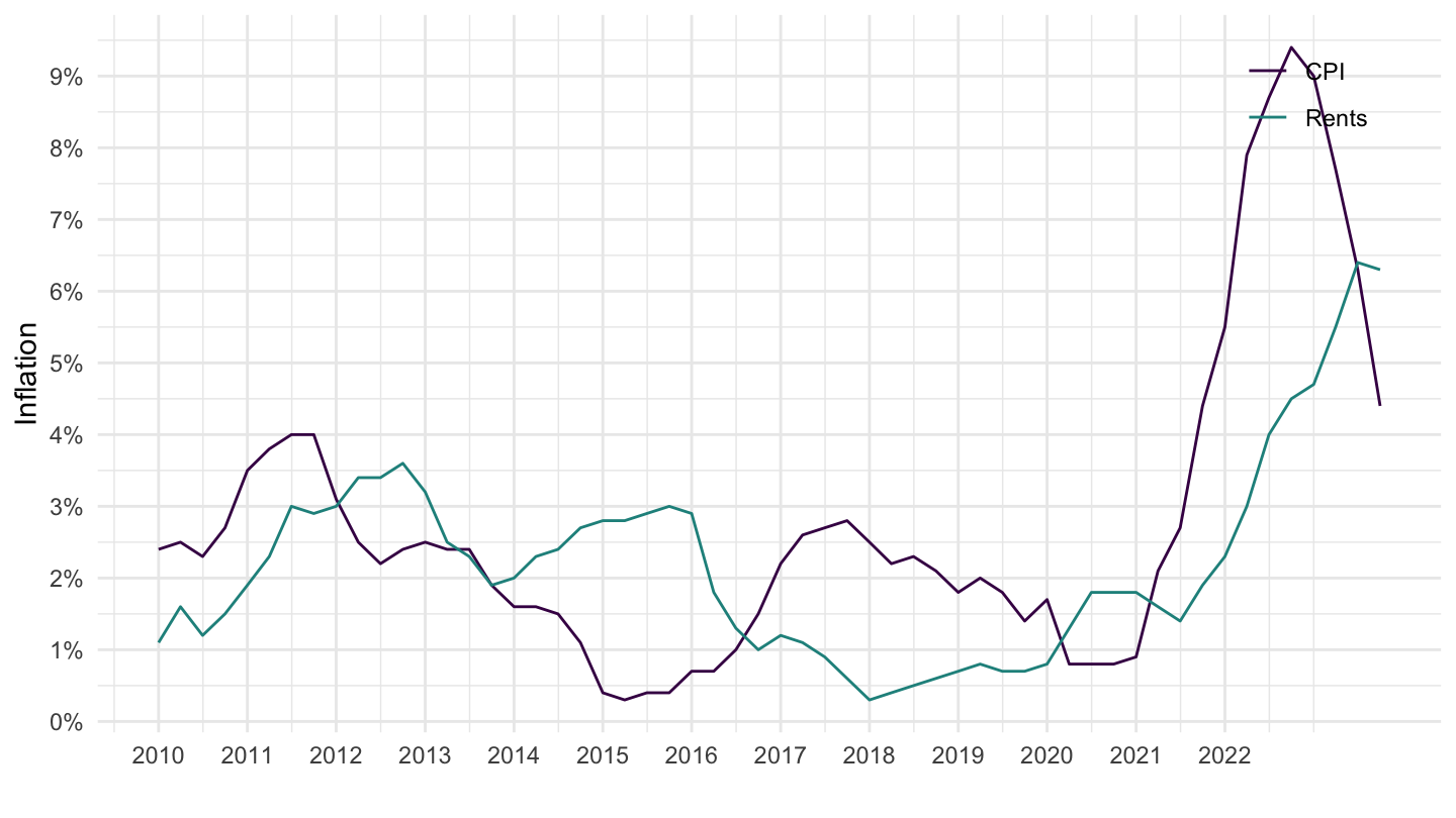
PRICES_CPI |>
  filter(LOCATION %in% c("GBR"),
         SUBJECT %in% c("CP040100", "CPALTT01"),
         FREQUENCY == "Q",
         MEASURE == "GY") |>
  quarter_to_date() |>
  select(SUBJECT, date, LOCATION, obsValue) |>
  spread(SUBJECT, obsValue) |>
  filter(!is.na(CP040100),
         date >= as.Date("2014-01-01"),
         date <= as.Date("2030-01-01")) |>
  mutate(rents_real = CP040100-CPALTT01) |>
  select(date, LOCATION, CPALTT01, CP040100) |>
  gather(variable, value, - date, -LOCATION) |>
  mutate(Variable = case_when(variable == "CP040100" ~ "Rents",
                              variable == "CPALTT01" ~ "CPI")) |>
  left_join(PRICES_CPI_var$LOCATION, by = "LOCATION") |>
  ggplot() + theme_minimal() + xlab("") + ylab("Inflation (%)") +
  geom_line(aes(x = date, y = value/100, color = Variable)) +
  scale_x_date(breaks = seq(1960, 2100, 1) |> paste0("-01-01") |> as.Date(),
               labels = date_format("%Y")) +
  scale_y_continuous(breaks = 0.01*seq(-100, 200, 0.5),
                     labels = percent_format(acc = .1)) +
  scale_color_manual(values = viridis(3)[1:2]) +
  theme(legend.position = c(0.9, 0.9),
        legend.title = element_blank())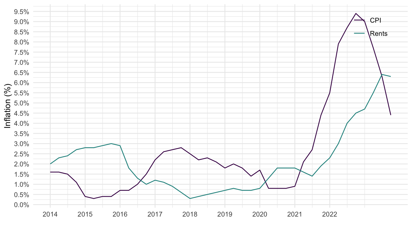
PRICES_CPI |>
  filter(LOCATION %in% c("CHE"),
         SUBJECT %in% c("CP040100", "CPALTT01"),
         FREQUENCY == "Q",
         MEASURE == "GY") |>
  quarter_to_date() |>
  select(SUBJECT, date, LOCATION, obsValue) |>
  spread(SUBJECT, obsValue) |>
  filter(!is.na(CP040100),
         date >= as.Date("1970-01-01")) |>
  mutate(rents_real = CP040100-CPALTT01) |>
  select(date, LOCATION, CPALTT01, CP040100) |>
  gather(variable, value, - date, -LOCATION) |>
  mutate(Variable = case_when(variable == "CP040100" ~ "Rents",
                              variable == "CPALTT01" ~ "CPI")) |>
  left_join(PRICES_CPI_var$LOCATION, by = "LOCATION") |>
  ggplot() + theme_minimal() + xlab("") + ylab("Inflation") +
  geom_line(aes(x = date, y = value/100, color = Variable)) +
  scale_x_date(breaks = seq(1960, 2100, 5) |> paste0("-01-01") |> as.Date(),
               labels = date_format("%Y")) +
  scale_y_continuous(breaks = 0.01*seq(-100, 200, 1),
                     labels = percent_format(acc = 1)) +
  scale_color_manual(values = viridis(3)[1:2]) +
  theme(legend.position = c(0.9, 0.9),
        legend.title = element_blank())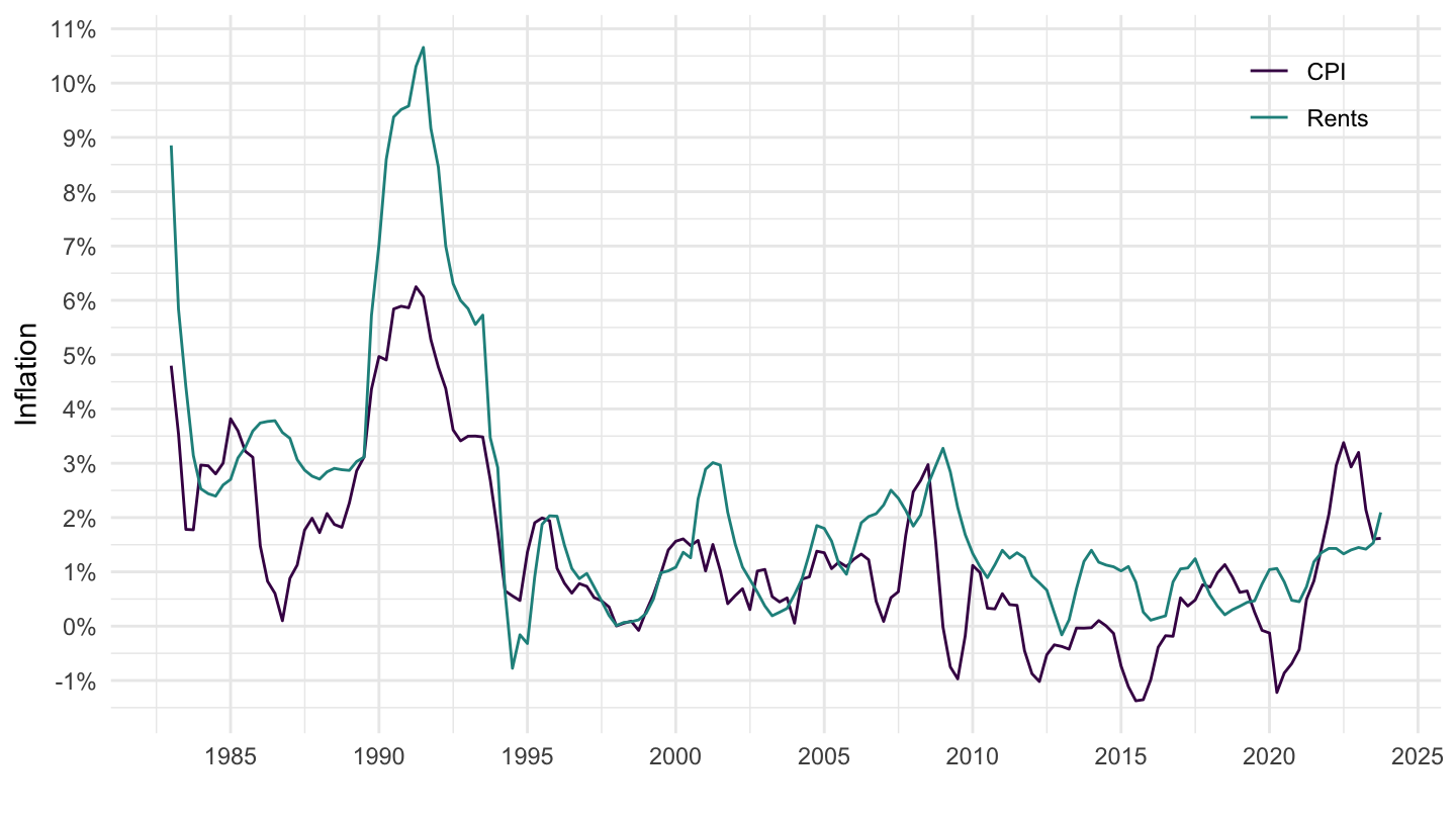
PRICES_CPI |>
  filter(LOCATION %in% c("USA"),
         SUBJECT %in% c("CP040100", "CPALTT01"),
         FREQUENCY == "Q",
         MEASURE == "GY") |>
  quarter_to_date() |>
  select(SUBJECT, date, LOCATION, obsValue) |>
  spread(SUBJECT, obsValue) |>
  filter(!is.na(CP040100),
         date >= as.Date("1970-01-01")) |>
  mutate(rents_real = CP040100-CPALTT01) |>
  select(date, LOCATION, CPALTT01, CP040100) |>
  gather(variable, value, - date, -LOCATION) |>
  mutate(Variable = case_when(variable == "CP040100" ~ "Rents",
                              variable == "CPALTT01" ~ "CPI")) |>
  left_join(PRICES_CPI_var$LOCATION, by = "LOCATION") |>
  ggplot() + theme_minimal() + xlab("") + ylab("Inflation") +
  geom_line(aes(x = date, y = value/100, color = Variable)) +
  scale_x_date(breaks = seq(1960, 2100, 5) |> paste0("-01-01") |> as.Date(),
               labels = date_format("%Y")) +
  scale_y_continuous(breaks = 0.01*seq(-100, 200, 1),
                     labels = percent_format(acc = 1)) +
  scale_color_manual(values = viridis(3)[1:2]) +
  theme(legend.position = c(0.9, 0.9),
        legend.title = element_blank())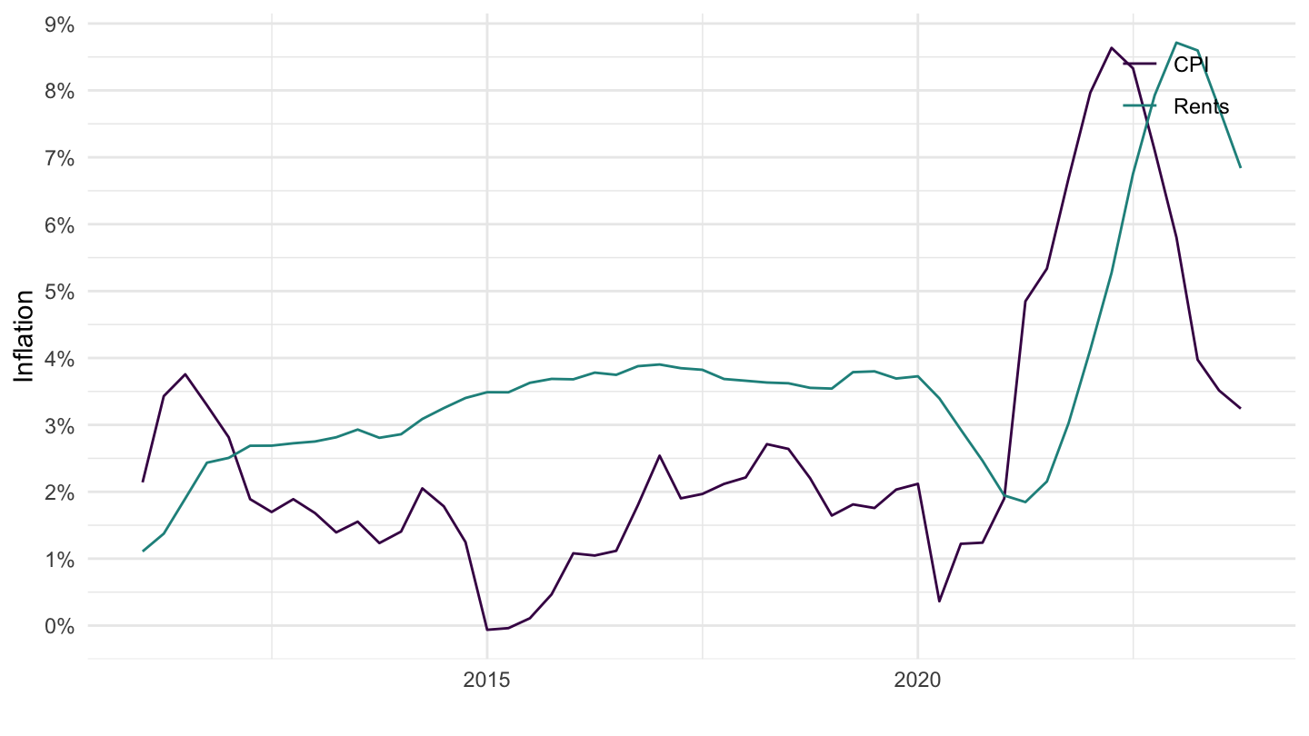
PRICES_CPI |>
  filter(LOCATION %in% c("FRA"),
         SUBJECT %in% c("CP040100", "CPALTT01"),
         FREQUENCY == "Q",
         MEASURE == "GY") |>
  quarter_to_date() |>
  select(SUBJECT, date, LOCATION, obsValue) |>
  spread(SUBJECT, obsValue) |>
  filter(!is.na(CP040100),
         date >= as.Date("1970-01-01")) |>
  mutate(rents_real = CP040100-CPALTT01) |>
  select(date, LOCATION, CPALTT01, CP040100) |>
  gather(variable, value, - date, -LOCATION) |>
  mutate(Variable = case_when(variable == "CP040100" ~ "Rents",
                              variable == "CPALTT01" ~ "CPI")) |>
  left_join(PRICES_CPI_var$LOCATION, by = "LOCATION") |>
  ggplot() + theme_minimal() + xlab("") + ylab("Inflation") +
  geom_line(aes(x = date, y = value/100, color = Variable)) +
  scale_x_date(breaks = seq(1960, 2100, 5) |> paste0("-01-01") |> as.Date(),
               labels = date_format("%Y")) +
  scale_y_continuous(breaks = 0.01*seq(-100, 200, 1),
                     labels = percent_format(acc = 1)) +
  scale_color_manual(values = viridis(3)[1:2]) +
  theme(legend.position = c(0.9, 0.9),
        legend.title = element_blank())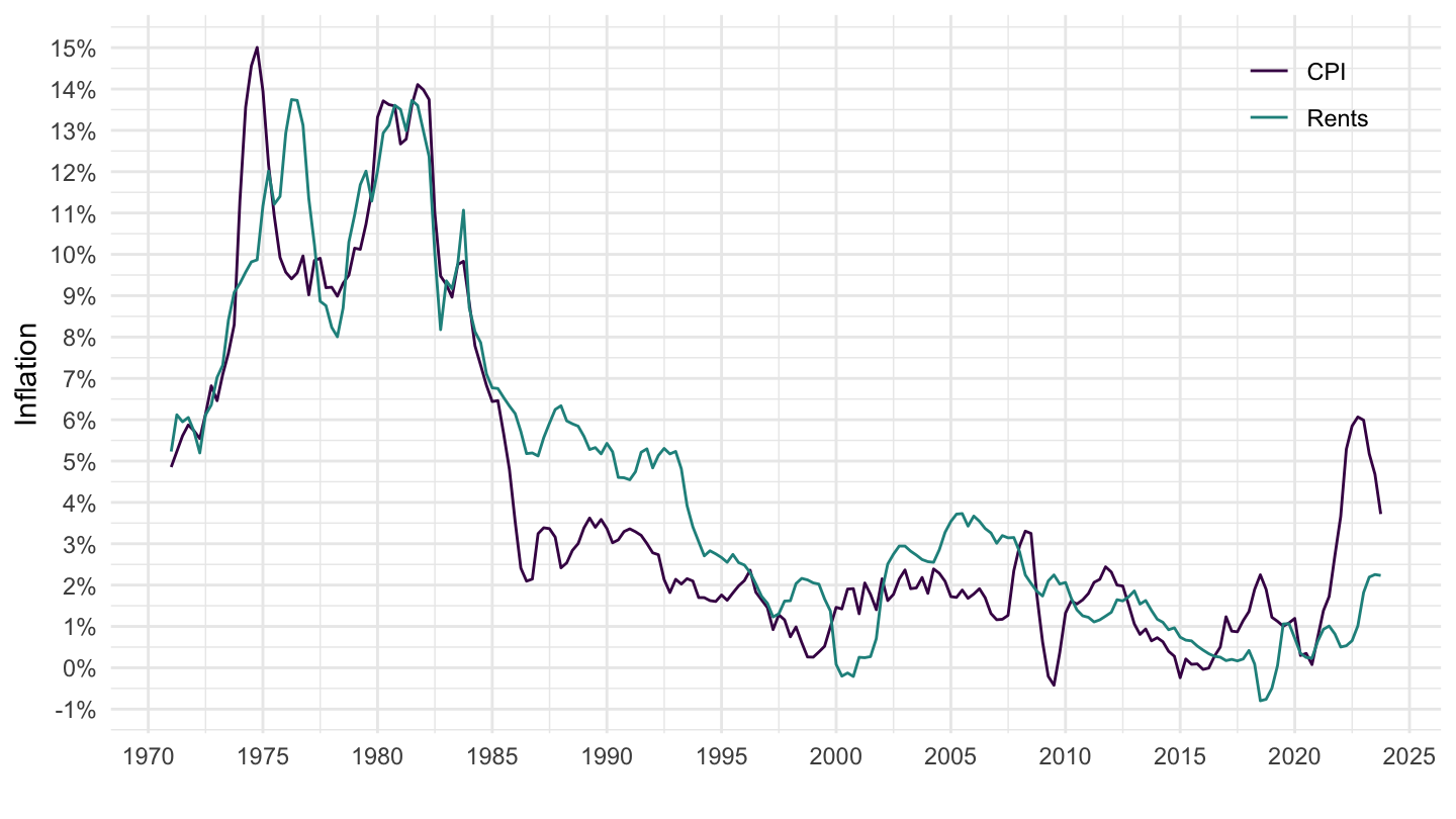
PRICES_CPI |>
  filter(LOCATION %in% c("AUS"),
         SUBJECT %in% c("CP040100", "CPALTT01"),
         FREQUENCY == "Q",
         MEASURE == "GY") |>
  quarter_to_date() |>
  select(SUBJECT, date, LOCATION, obsValue) |>
  spread(SUBJECT, obsValue) |>
  filter(!is.na(CP040100),
         date >= as.Date("1970-01-01")) |>
  mutate(rents_real = CP040100-CPALTT01) |>
  select(date, LOCATION, CPALTT01, CP040100) |>
  gather(variable, value, - date, -LOCATION) |>
  mutate(Variable = case_when(variable == "CP040100" ~ "Rents",
                              variable == "CPALTT01" ~ "CPI")) |>
  left_join(PRICES_CPI_var$LOCATION, by = "LOCATION") |>
  ggplot() + theme_minimal() + xlab("") + ylab("Inflation") +
  geom_line(aes(x = date, y = value/100, color = Variable)) +
  scale_x_date(breaks = seq(1960, 2100, 5) |> paste0("-01-01") |> as.Date(),
               labels = date_format("%Y")) +
  scale_y_continuous(breaks = 0.01*seq(-100, 200, 1),
                     labels = percent_format(acc = 1)) +
  scale_color_manual(values = viridis(3)[1:2]) +
  theme(legend.position = c(0.9, 0.9),
        legend.title = element_blank())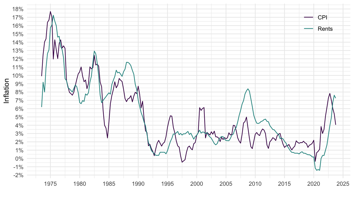
PRICES_CPI |>
  filter(LOCATION %in% c("ISL"),
         SUBJECT %in% c("CP040100", "CPALTT01"),
         FREQUENCY == "Q",
         MEASURE == "IXOB") |>
  quarter_to_date() |>
  select(SUBJECT, date, LOCATION, obsValue) |>
  spread(SUBJECT, obsValue) |>
  filter(!is.na(CP040100)) |>
  mutate(rents_real = 100*CP040100/CPALTT01) |>
  select(date, LOCATION, CPALTT01, rents_real, CP040100) |>
  gather(variable, value, - date, -LOCATION) |>
  mutate(Variable = case_when(variable == "rents_real" ~ "Real Rents",
                              variable == "CP040100" ~ "Rents",
                              variable == "CPALTT01" ~ "CPI")) |>
  left_join(PRICES_CPI_var$LOCATION, by = "LOCATION") |>
  ggplot() + theme_minimal() + xlab("") + ylab("CPI") +
  geom_line(aes(x = date, y = value, color = Variable, linetype = Variable)) +
  scale_x_date(breaks = seq(1960, 2100, 2) |> paste0("-01-01") |> as.Date(),
               labels = date_format("%Y")) +
  scale_y_log10(breaks = seq(0, 200, 5)) +
  scale_color_manual(values = viridis(4)[1:3]) +
  theme(legend.position = c(0.7, 0.30),
        legend.title = element_blank())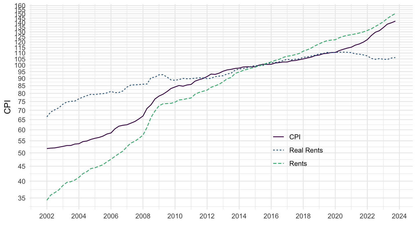
PRICES_CPI |>
  filter(LOCATION %in% c("ISL"),
         SUBJECT %in% c("CP040100", "CPALTT01"),
         FREQUENCY == "Q",
         MEASURE == "IXOB") |>
  quarter_to_date() |>
  filter(date >= as.Date("2007-01-01")) |>
  select(SUBJECT, date, LOCATION, obsValue) |>
  spread(SUBJECT, obsValue) |>
  filter(!is.na(CP040100)) |>
  mutate(CP040100 = 100*CP040100/CP040100[date == as.Date("2007-01-01")],
         CPALTT01 = 100*CPALTT01/CPALTT01[date == as.Date("2007-01-01")],
         rents_real = 100*CP040100/CPALTT01) |>
  select(date, LOCATION, CPALTT01, rents_real, CP040100) |>
  gather(variable, value, - date, -LOCATION) |>
  mutate(Variable = case_when(variable == "rents_real" ~ "Real Rents",
                              variable == "CP040100" ~ "Rents",
                              variable == "CPALTT01" ~ "CPI")) |>
  ggplot() + theme_minimal() + xlab("") + ylab("CPI") +
  geom_line(aes(x = date, y = value, color = Variable, linetype = Variable)) +
  scale_x_date(breaks = seq(1960, 2100, 2) |> paste0("-01-01") |> as.Date(),
               labels = date_format("%Y")) +
  scale_y_log10(breaks = seq(0, 400, 20)) +
  scale_color_manual(values = viridis(4)[1:3]) +
  theme(legend.position = c(0.2, 0.8),
        legend.title = element_blank())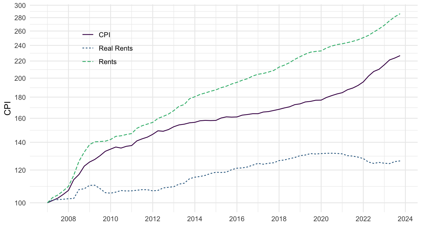
PRICES_CPI |>
  filter(LOCATION %in% c("JPN"),
         SUBJECT %in% c("CP040100", "CPALTT01"),
         FREQUENCY == "Q",
         MEASURE == "IXOB") |>
  quarter_to_date() |>
  select(SUBJECT, date, LOCATION, obsValue) |>
  spread(SUBJECT, obsValue) |>
  filter(!is.na(CP040100)) |>
  mutate(rents_real = 100*CP040100/CPALTT01) |>
  select(date, LOCATION, CPALTT01, rents_real, CP040100) |>
  gather(variable, value, - date, -LOCATION) |>
  mutate(Variable = case_when(variable == "rents_real" ~ "Real Rents",
                              variable == "CP040100" ~ "Rents",
                              variable == "CPALTT01" ~ "CPI")) |>
  left_join(PRICES_CPI_var$LOCATION, by = "LOCATION") |>
  ggplot() + theme_minimal() + xlab("") + ylab("CPI") +
  geom_line(aes(x = date, y = value, color = Variable, linetype = Variable)) +
  scale_x_date(breaks = seq(1960, 2100, 5) |> paste0("-01-01") |> as.Date(),
               labels = date_format("%Y")) +
  scale_y_log10(breaks = seq(0, 200, 5)) +
  scale_color_manual(values = viridis(4)[1:3]) +
  theme(legend.position = c(0.7, 0.30),
        legend.title = element_blank())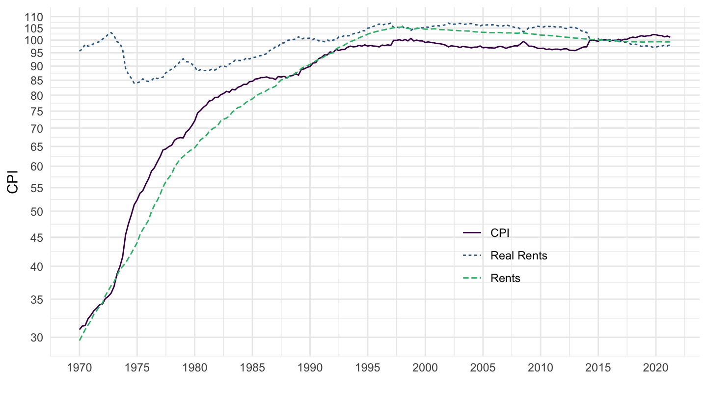
PRICES_CPI |>
  filter(LOCATION %in% c("JPN"),
         SUBJECT %in% c("CP040100", "CPALTT01"),
         FREQUENCY == "Q",
         MEASURE == "IXOB") |>
  quarter_to_date() |>
  filter(date >= as.Date("1980-01-01")) |>
  select(SUBJECT, date, LOCATION, obsValue) |>
  spread(SUBJECT, obsValue) |>
  filter(!is.na(CP040100)) |>
  mutate(rents_real = 100*CP040100/CPALTT01) |>
  select(date, LOCATION, CPALTT01, rents_real, CP040100) |>
  gather(variable, value, - date, -LOCATION) |>
  mutate(Variable = case_when(variable == "rents_real" ~ "Real Rents",
                              variable == "CP040100" ~ "Rents",
                              variable == "CPALTT01" ~ "CPI")) |>
  left_join(PRICES_CPI_var$LOCATION, by = "LOCATION") |>
  ggplot() + theme_minimal() + xlab("") + ylab("CPI") +
  geom_line(aes(x = date, y = value, color = Variable, linetype = Variable)) +
  scale_x_date(breaks = seq(1960, 2100, 5) |> paste0("-01-01") |> as.Date(),
               labels = date_format("%Y")) +
  scale_y_log10(breaks = seq(0, 200, 5)) +
  scale_color_manual(values = viridis(4)[1:3]) +
  theme(legend.position = c(0.7, 0.30),
        legend.title = element_blank())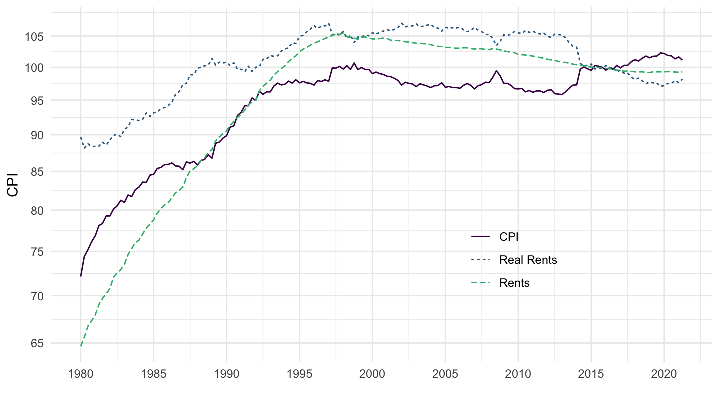
PRICES_CPI |>
  filter(LOCATION %in% c("JPN"),
         SUBJECT %in% c("CP040100", "CPALTT01"),
         FREQUENCY == "Q",
         MEASURE == "IXOB") |>
  quarter_to_date() |>
  filter(date >= as.Date("1980-01-01"),
         date <= as.Date("2000-01-01")) |>
  select(SUBJECT, date, LOCATION, obsValue) |>
  spread(SUBJECT, obsValue) |>
  filter(!is.na(CP040100)) |>
  mutate(rents_real = 100*CP040100/CPALTT01) |>
  select(date, LOCATION, CPALTT01, rents_real, CP040100) |>
  gather(variable, value, - date, -LOCATION) |>
  mutate(Variable = case_when(variable == "rents_real" ~ "Real Rents",
                              variable == "CP040100" ~ "Rents",
                              variable == "CPALTT01" ~ "CPI")) |>
  left_join(PRICES_CPI_var$LOCATION, by = "LOCATION") |>
  ggplot() + theme_minimal() + xlab("") + ylab("CPI") +
  geom_line(aes(x = date, y = value, color = Variable, linetype = Variable)) +
  scale_x_date(breaks = seq(1960, 2100, 2) |> paste0("-01-01") |> as.Date(),
               labels = date_format("%Y")) +
  scale_y_log10(breaks = seq(0, 200, 5)) +
  scale_color_manual(values = viridis(4)[1:3]) +
  theme(legend.position = c(0.7, 0.30),
        legend.title = element_blank())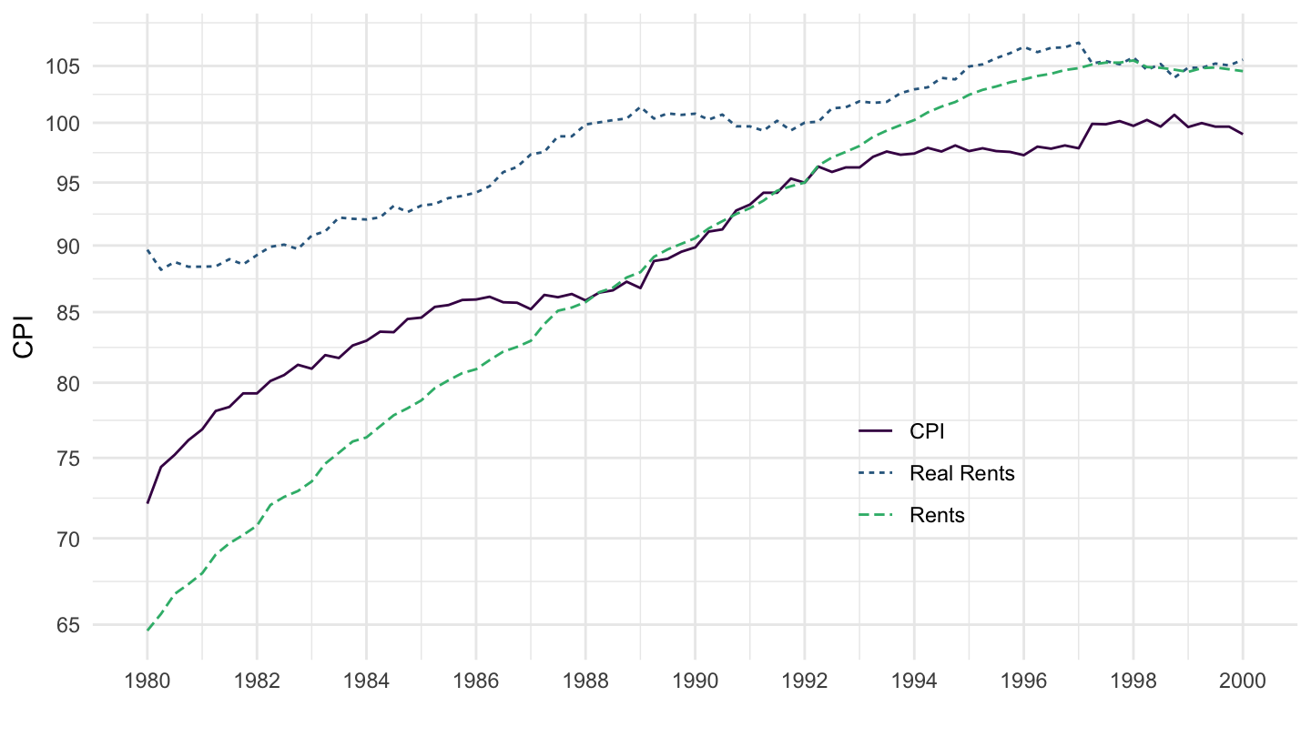
PRICES_CPI |>
  filter(LOCATION %in% c("JPN"),
         SUBJECT %in% c("CP040100", "CPALTT01"),
         FREQUENCY == "Q",
         MEASURE == "IXOB") |>
  quarter_to_date() |>
  filter(date >= as.Date("2000-01-01")) |>
  select(SUBJECT, date, LOCATION, obsValue) |>
  spread(SUBJECT, obsValue) |>
  filter(!is.na(CP040100)) |>
  mutate(rents_real = 100*CP040100/CPALTT01) |>
  select(date, LOCATION, CPALTT01, rents_real, CP040100) |>
  gather(variable, value, - date, -LOCATION) |>
  mutate(Variable = case_when(variable == "rents_real" ~ "Real Rents",
                              variable == "CP040100" ~ "Rents",
                              variable == "CPALTT01" ~ "CPI")) |>
  left_join(PRICES_CPI_var$LOCATION, by = "LOCATION") |>
  ggplot() + theme_minimal() + xlab("") + ylab("CPI") +
  geom_line(aes(x = date, y = value, color = Variable, linetype = Variable)) +
  scale_x_date(breaks = seq(1960, 2100, 2) |> paste0("-01-01") |> as.Date(),
               labels = date_format("%Y")) +
  scale_y_log10(breaks = seq(0, 200, 1)) +
  scale_color_manual(values = viridis(4)[1:3]) +
  theme(legend.position = c(0.8, 0.8),
        legend.title = element_blank())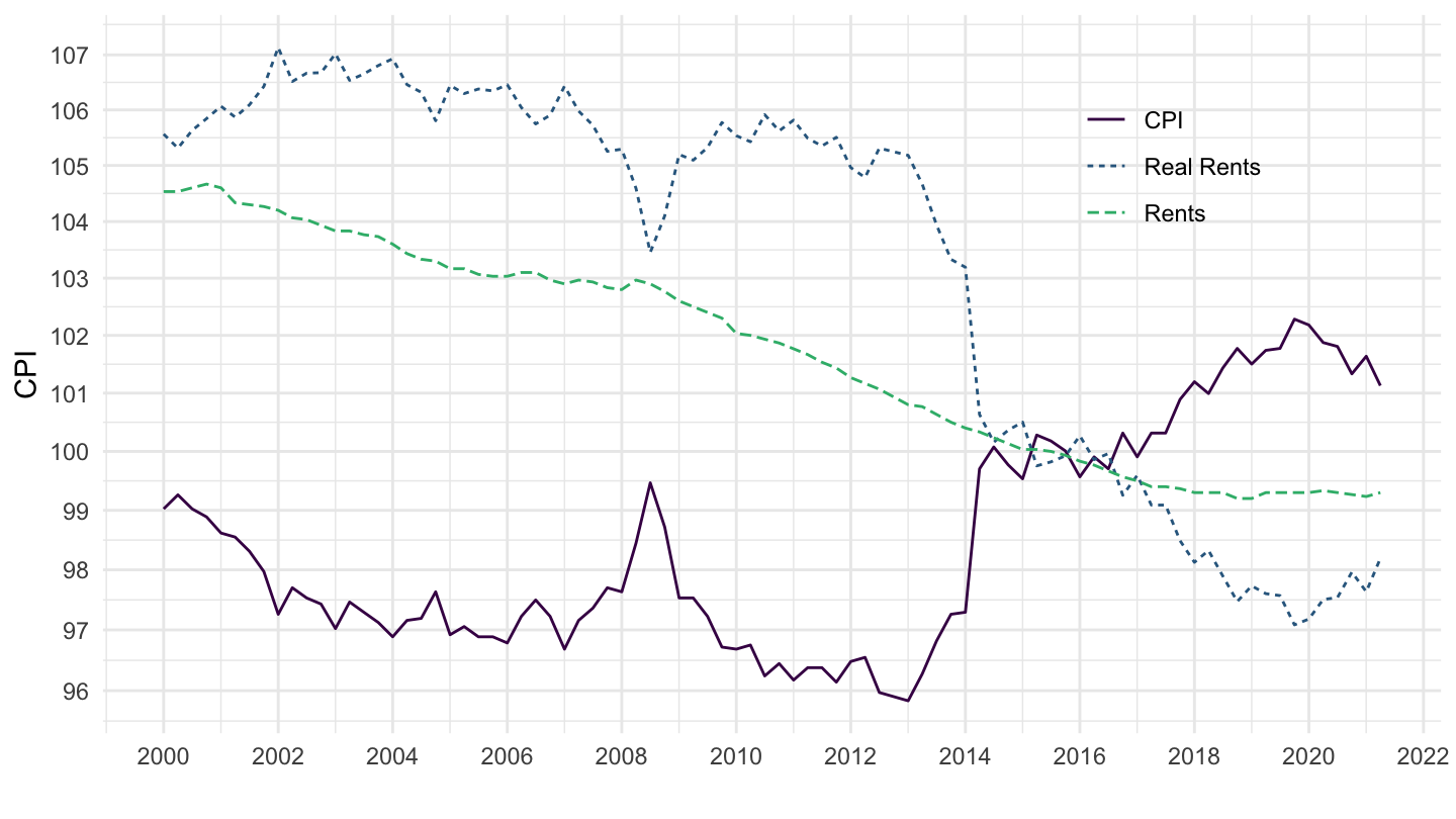
PRICES_CPI |>
  filter(LOCATION %in% c("JPN"),
         SUBJECT %in% c("CP040100", "CPALTT01"),
         FREQUENCY == "M",
         MEASURE == "IXOB") |>
  month_to_date() |>
  filter(date >= as.Date("2010-01-01")) |>
  select(SUBJECT, date, LOCATION, obsValue) |>
  spread(SUBJECT, obsValue) |>
  filter(!is.na(CP040100)) |>
  mutate(rents_real = 100*CP040100/CPALTT01) |>
  select(date, LOCATION, CPALTT01, rents_real, CP040100) |>
  gather(variable, value, - date, -LOCATION) |>
  mutate(Variable = case_when(variable == "rents_real" ~ "Real Rents",
                              variable == "CP040100" ~ "Rents",
                              variable == "CPALTT01" ~ "CPI")) |>
  left_join(PRICES_CPI_var$LOCATION, by = "LOCATION") |>
  ggplot() + theme_minimal() + xlab("") + ylab("CPI") +
  geom_line(aes(x = date, y = value, color = Variable, linetype = Variable)) +
  scale_x_date(breaks = seq(1960, 2100, 1) |> paste0("-01-01") |> as.Date(),
               labels = date_format("%Y")) +
  scale_y_log10(breaks = seq(0, 200, 1)) +
  scale_color_manual(values = viridis(4)[1:3]) +
  theme(legend.position = c(0.7, 0.80),
        legend.title = element_blank())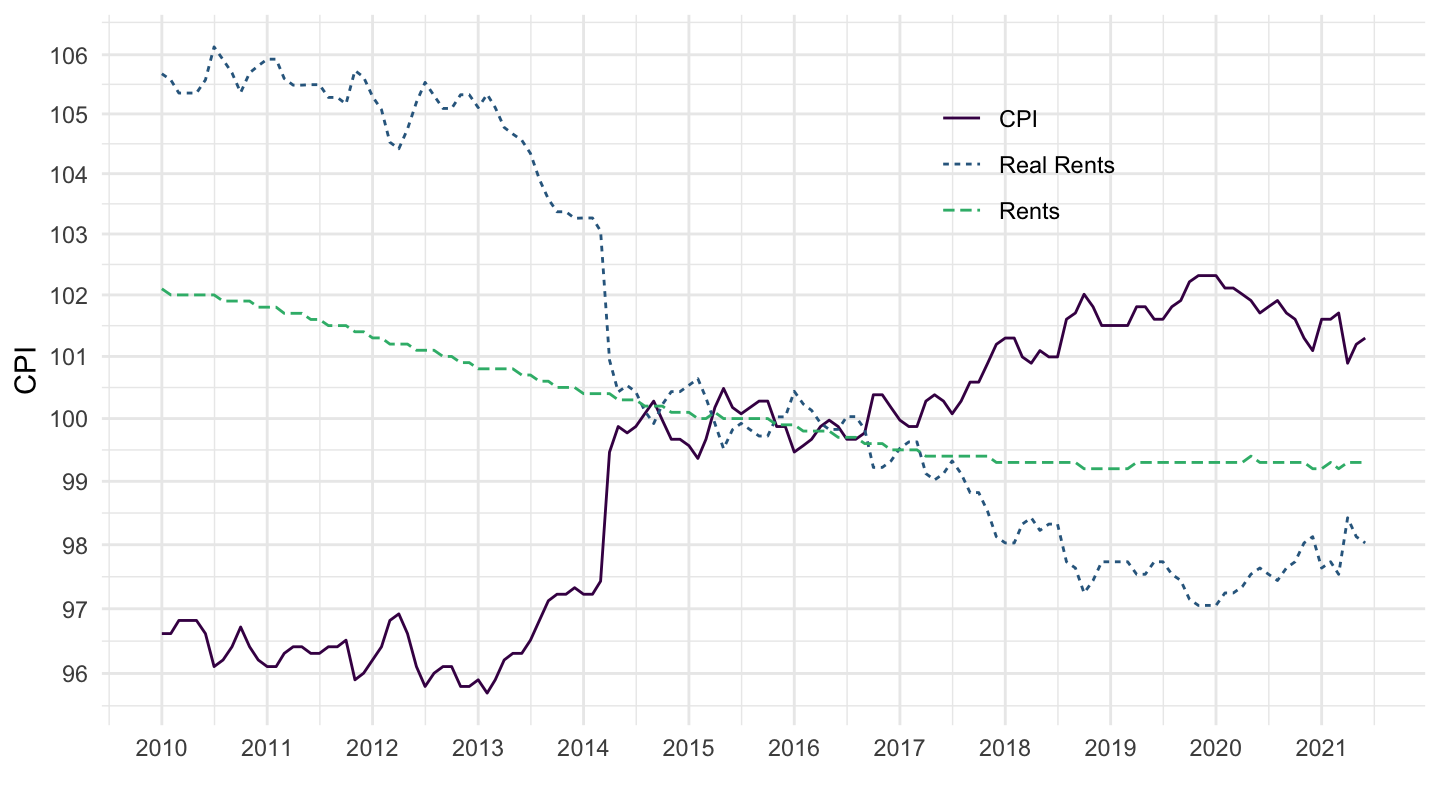
PRICES_CPI |>
  filter(LOCATION %in% c("GBR"),
         SUBJECT %in% c("CP040100", "CPALTT01"),
         FREQUENCY == "Q",
         MEASURE == "IXOB") |>
  quarter_to_date() |>
  filter(date >= as.Date("1980-01-01")) |>
  select(SUBJECT, date, LOCATION, obsValue) |>
  spread(SUBJECT, obsValue) |>
  filter(!is.na(CP040100)) |>
  mutate(rents_real = 100*CP040100/CPALTT01) |>
  select(date, LOCATION, CPALTT01, rents_real, CP040100) |>
  gather(variable, value, - date, -LOCATION) |>
  mutate(Variable = case_when(variable == "rents_real" ~ "Real Rents",
                              variable == "CP040100" ~ "Rents",
                              variable == "CPALTT01" ~ "CPI")) |>
  left_join(PRICES_CPI_var$LOCATION, by = "LOCATION") |>
  ggplot() + theme_minimal() + xlab("") + ylab("CPI") +
  geom_line(aes(x = date, y = value, color = Variable, linetype = Variable)) +
  scale_x_date(breaks = seq(1960, 2100, 5) |> paste0("-01-01") |> as.Date(),
               labels = date_format("%Y")) +
  scale_y_log10(breaks = seq(0, 200, 5)) +
  scale_color_manual(values = viridis(4)[1:3]) +
  theme(legend.position = c(0.7, 0.30),
        legend.title = element_blank())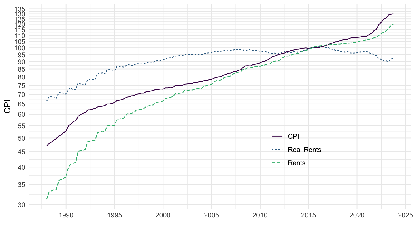
PRICES_CPI |>
  filter(LOCATION %in% c("GBR"),
         SUBJECT %in% c("CP040100", "CPALTT01"),
         FREQUENCY == "Q",
         MEASURE == "IXOB") |>
  quarter_to_date() |>
  filter(date >= as.Date("2000-01-01")) |>
  select(SUBJECT, date, LOCATION, obsValue) |>
  spread(SUBJECT, obsValue) |>
  filter(!is.na(CP040100)) |>
  mutate(rents_real = 100*CP040100/CPALTT01) |>
  select(date, LOCATION, CPALTT01, rents_real, CP040100) |>
  gather(variable, value, - date, -LOCATION) |>
  mutate(Variable = case_when(variable == "rents_real" ~ "Real Rents",
                              variable == "CP040100" ~ "Rents",
                              variable == "CPALTT01" ~ "CPI")) |>
  left_join(PRICES_CPI_var$LOCATION, by = "LOCATION") |>
  ggplot() + theme_minimal() + xlab("") + ylab("CPI") +
  geom_line(aes(x = date, y = value, color = Variable, linetype = Variable)) +
  scale_x_date(breaks = seq(1960, 2100, 5) |> paste0("-01-01") |> as.Date(),
               labels = date_format("%Y")) +
  scale_y_log10(breaks = seq(0, 200, 5)) +
  scale_color_manual(values = viridis(4)[1:3]) +
  theme(legend.position = c(0.7, 0.30),
        legend.title = element_blank())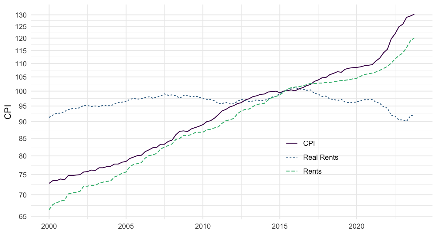
PRICES_CPI |>
  filter(LOCATION %in% c("ISR"),
         SUBJECT %in% c("CP040100", "CPALTT01"),
         FREQUENCY == "Q",
         MEASURE == "IXOB") |>
  quarter_to_date() |>
  filter(date >= as.Date("1980-01-01")) |>
  select(SUBJECT, date, LOCATION, obsValue) |>
  spread(SUBJECT, obsValue) |>
  filter(!is.na(CP040100)) |>
  mutate(rents_real = 100*CP040100/CPALTT01) |>
  select(date, LOCATION, CPALTT01, rents_real, CP040100) |>
  gather(variable, value, - date, -LOCATION) |>
  mutate(Variable = case_when(variable == "rents_real" ~ "Real Rents",
                              variable == "CP040100" ~ "Rents",
                              variable == "CPALTT01" ~ "CPI")) |>
  left_join(PRICES_CPI_var$LOCATION, by = "LOCATION") |>
  ggplot() + theme_minimal() + xlab("") + ylab("CPI") +
  geom_line(aes(x = date, y = value, color = Variable, linetype = Variable)) +
  scale_x_date(breaks = seq(1960, 2100, 5) |> paste0("-01-01") |> as.Date(),
               labels = date_format("%Y")) +
  scale_y_log10(breaks = seq(0, 200, 5)) +
  scale_color_manual(values = viridis(4)[1:3]) +
  theme(legend.position = c(0.7, 0.30),
        legend.title = element_blank())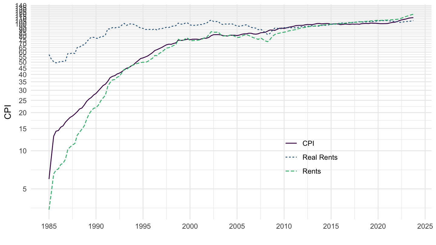
PRICES_CPI |>
  filter(LOCATION %in% c("ISR"),
         SUBJECT %in% c("CP040100", "CPALTT01"),
         FREQUENCY == "Q",
         MEASURE == "IXOB") |>
  quarter_to_date() |>
  filter(date >= as.Date("2000-01-01")) |>
  select(SUBJECT, date, LOCATION, obsValue) |>
  spread(SUBJECT, obsValue) |>
  filter(!is.na(CP040100)) |>
  mutate(rents_real = 100*CP040100/CPALTT01) |>
  select(date, LOCATION, CPALTT01, rents_real, CP040100) |>
  gather(variable, value, - date, -LOCATION) |>
  mutate(Variable = case_when(variable == "rents_real" ~ "Real Rents",
                              variable == "CP040100" ~ "Rents",
                              variable == "CPALTT01" ~ "CPI")) |>
  left_join(PRICES_CPI_var$LOCATION, by = "LOCATION") |>
  ggplot() + theme_minimal() + xlab("") + ylab("CPI") +
  geom_line(aes(x = date, y = value, color = Variable, linetype = Variable)) +
  scale_x_date(breaks = seq(1960, 2100, 2) |> paste0("-01-01") |> as.Date(),
               labels = date_format("%Y")) +
  scale_y_log10(breaks = seq(0, 200, 5)) +
  scale_color_manual(values = viridis(4)[1:3]) +
  theme(legend.position = c(0.7, 0.30),
        legend.title = element_blank())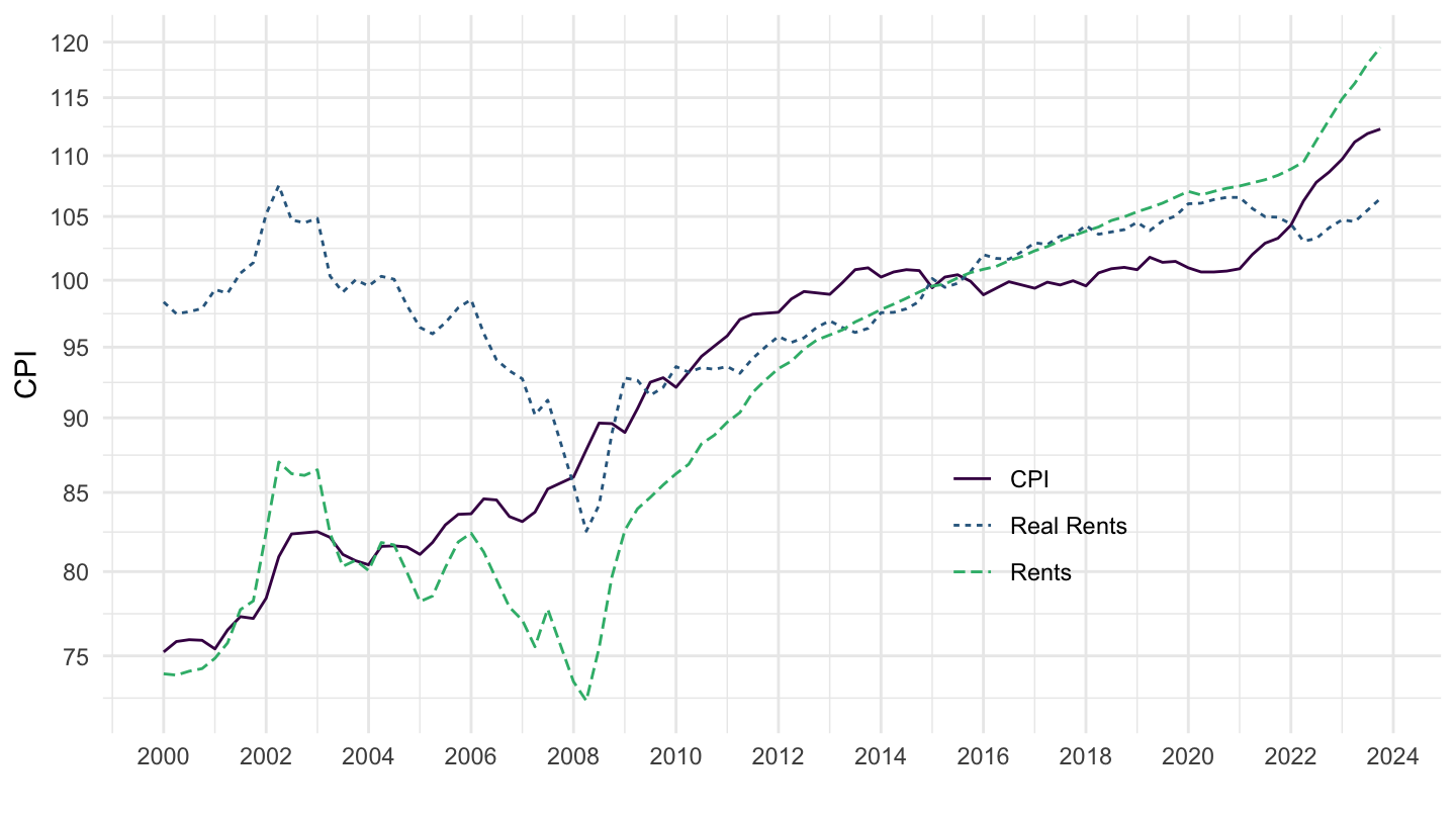
PRICES_CPI |>
  filter(LOCATION %in% c("ISR"),
         SUBJECT %in% c("CP040100", "CPALTT01"),
         FREQUENCY == "M",
         MEASURE == "IXOB") |>
  month_to_date() |>
  filter(date >= as.Date("2010-01-01")) |>
  select(SUBJECT, date, LOCATION, obsValue) |>
  spread(SUBJECT, obsValue) |>
  filter(!is.na(CP040100)) |>
  mutate(rents_real = 100*CP040100/CPALTT01) |>
  select(date, LOCATION, CPALTT01, rents_real, CP040100) |>
  gather(variable, value, - date, -LOCATION) |>
  mutate(Variable = case_when(variable == "rents_real" ~ "Real Rents",
                              variable == "CP040100" ~ "Rents",
                              variable == "CPALTT01" ~ "CPI")) |>
  left_join(PRICES_CPI_var$LOCATION, by = "LOCATION") |>
  ggplot() + theme_minimal() + xlab("") + ylab("CPI") +
  geom_line(aes(x = date, y = value, color = Variable, linetype = Variable)) +
  scale_x_date(breaks = seq(1960, 2100, 1) |> paste0("-01-01") |> as.Date(),
               labels = date_format("%Y")) +
  scale_y_log10(breaks = seq(0, 200, 1)) +
  scale_color_manual(values = viridis(4)[1:3]) +
  theme(legend.position = c(0.7, 0.30),
        legend.title = element_blank())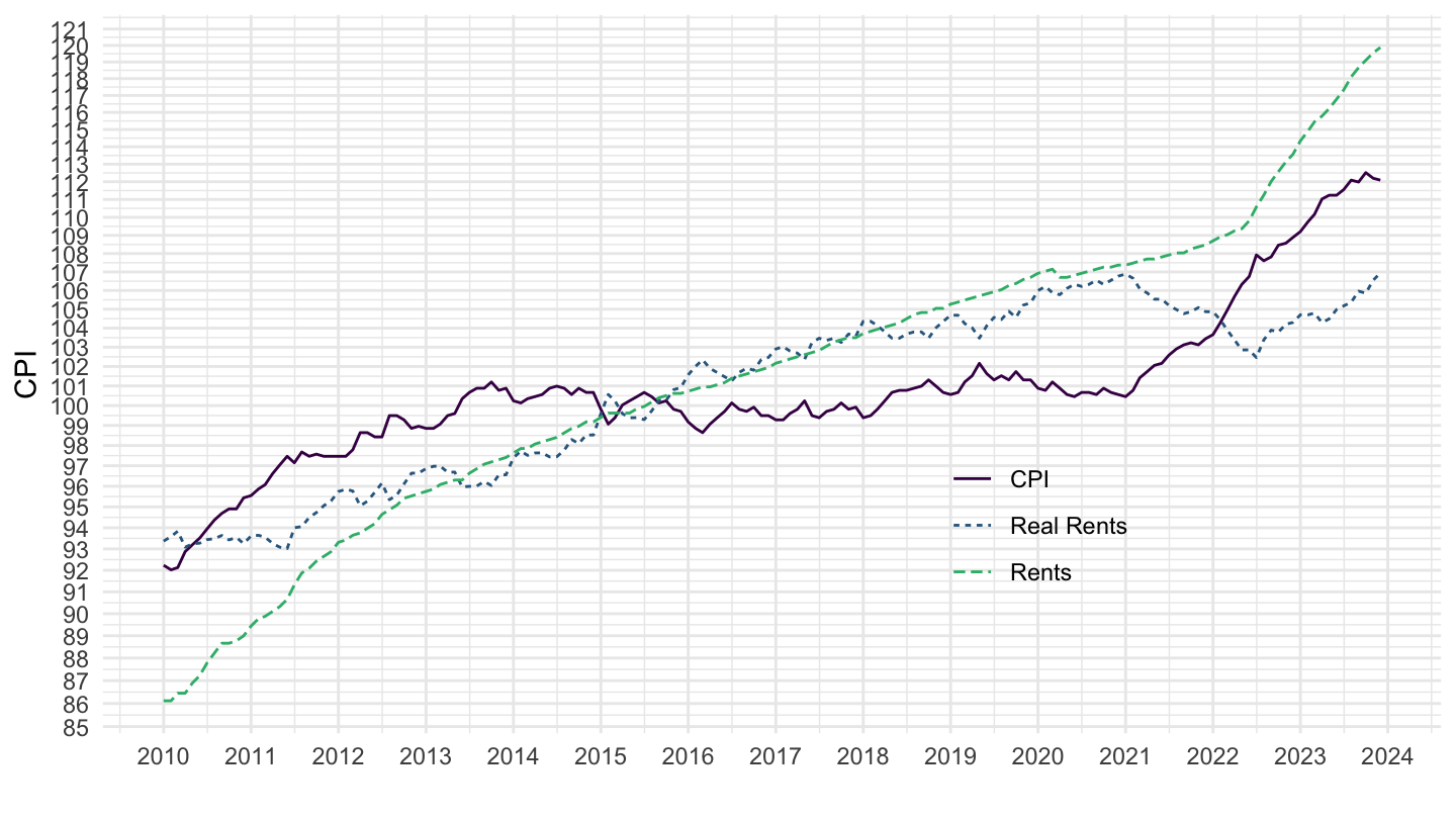
PRICES_CPI |>
  filter(LOCATION %in% c("CHE"),
         SUBJECT %in% c("CP040100", "CPALTT01"),
         FREQUENCY == "Q",
         MEASURE == "IXOB") |>
  quarter_to_date() |>
  filter(date >= as.Date("1980-01-01")) |>
  select(SUBJECT, date, LOCATION, obsValue) |>
  spread(SUBJECT, obsValue) |>
  filter(!is.na(CP040100)) |>
  mutate(rents_real = 100*CP040100/CPALTT01) |>
  select(date, LOCATION, CPALTT01, rents_real, CP040100) |>
  gather(variable, value, - date, -LOCATION) |>
  mutate(Variable = case_when(variable == "rents_real" ~ "Real Rents",
                              variable == "CP040100" ~ "Rents",
                              variable == "CPALTT01" ~ "CPI")) |>
  left_join(PRICES_CPI_var$LOCATION, by = "LOCATION") |>
  ggplot() + theme_minimal() + xlab("") + ylab("CPI") +
  geom_line(aes(x = date, y = value, color = Variable, linetype = Variable)) +
  scale_x_date(breaks = seq(1960, 2100, 5) |> paste0("-01-01") |> as.Date(),
               labels = date_format("%Y")) +
  scale_y_log10(breaks = seq(0, 200, 5)) +
  scale_color_manual(values = viridis(4)[1:3]) +
  theme(legend.position = c(0.7, 0.30),
        legend.title = element_blank())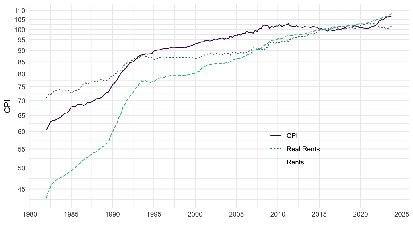
PRICES_CPI |>
  filter(LOCATION %in% c("CHE"),
         SUBJECT %in% c("CP040100", "CPALTT01"),
         FREQUENCY == "Q",
         MEASURE == "IXOB") |>
  quarter_to_date() |>
  filter(date >= as.Date("2000-01-01")) |>
  select(SUBJECT, date, LOCATION, obsValue) |>
  spread(SUBJECT, obsValue) |>
  filter(!is.na(CP040100)) |>
  mutate(rents_real = 100*CP040100/CPALTT01) |>
  select(date, LOCATION, CPALTT01, rents_real, CP040100) |>
  gather(variable, value, - date, -LOCATION) |>
  mutate(Variable = case_when(variable == "rents_real" ~ "Real Rents",
                              variable == "CP040100" ~ "Rents",
                              variable == "CPALTT01" ~ "CPI")) |>
  left_join(PRICES_CPI_var$LOCATION, by = "LOCATION") |>
  ggplot() + theme_minimal() + xlab("") + ylab("CPI") +
  geom_line(aes(x = date, y = value, color = Variable, linetype = Variable)) +
  scale_x_date(breaks = seq(1960, 2100, 2) |> paste0("-01-01") |> as.Date(),
               labels = date_format("%Y")) +
  scale_y_log10(breaks = seq(0, 200, 5)) +
  scale_color_manual(values = viridis(4)[1:3]) +
  theme(legend.position = c(0.7, 0.30),
        legend.title = element_blank())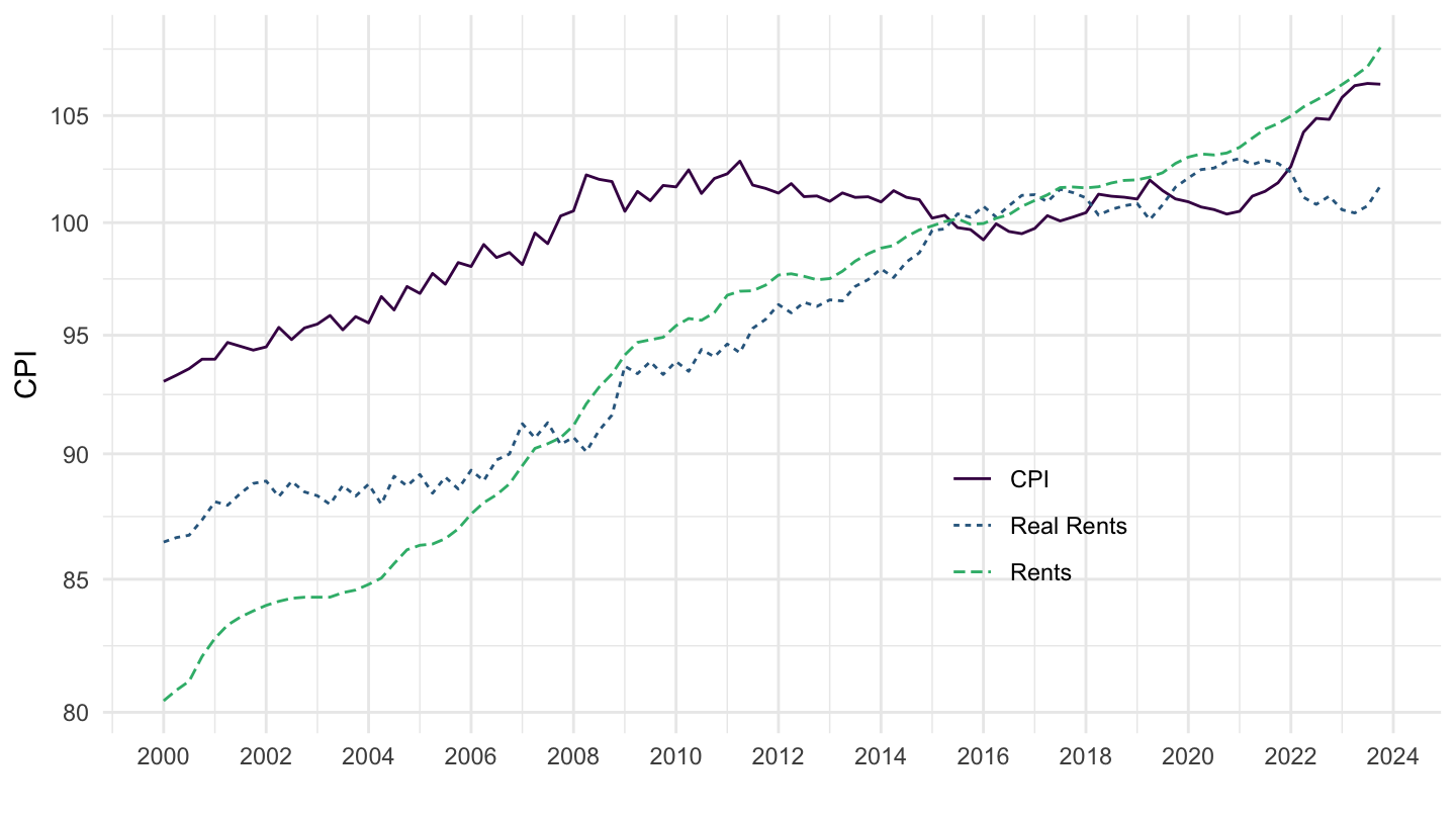
PRICES_CPI |>
  filter(LOCATION %in% c("CHE"),
         SUBJECT %in% c("CP040100", "CPALTT01"),
         FREQUENCY == "M",
         MEASURE == "IXOB") |>
  month_to_date() |>
  filter(date >= as.Date("2010-01-01")) |>
  select(SUBJECT, date, LOCATION, obsValue) |>
  spread(SUBJECT, obsValue) |>
  filter(!is.na(CP040100)) |>
  mutate(rents_real = 100*CP040100/CPALTT01) |>
  select(date, LOCATION, CPALTT01, rents_real, CP040100) |>
  gather(variable, value, - date, -LOCATION) |>
  mutate(Variable = case_when(variable == "rents_real" ~ "Real Rents",
                              variable == "CP040100" ~ "Rents",
                              variable == "CPALTT01" ~ "CPI")) |>
  left_join(PRICES_CPI_var$LOCATION, by = "LOCATION") |>
  ggplot() + theme_minimal() + xlab("") + ylab("CPI") +
  geom_line(aes(x = date, y = value, color = Variable, linetype = Variable)) +
  scale_x_date(breaks = seq(1960, 2100, 1) |> paste0("-01-01") |> as.Date(),
               labels = date_format("%Y")) +
  scale_y_log10(breaks = seq(0, 200, 1)) +
  scale_color_manual(values = viridis(4)[1:3]) +
  theme(legend.position = c(0.7, 0.30),
        legend.title = element_blank())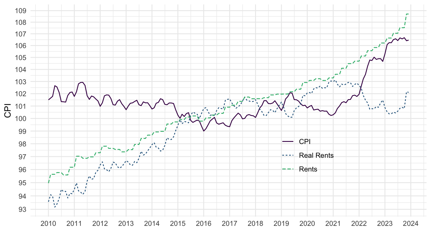
PRICES_CPI |>
  filter(LOCATION %in% c("FRA"),
         SUBJECT %in% c("CP040100", "CPALTT01"),
         FREQUENCY == "Q",
         MEASURE == "IXOB") |>
  quarter_to_date() |>
  filter(date >= as.Date("1980-01-01")) |>
  select(SUBJECT, date, LOCATION, obsValue) |>
  spread(SUBJECT, obsValue) |>
  filter(!is.na(CP040100)) |>
  mutate(rents_real = 100*CP040100/CPALTT01) |>
  select(date, LOCATION, CPALTT01, rents_real, CP040100) |>
  gather(variable, value, - date, -LOCATION) |>
  mutate(Variable = case_when(variable == "rents_real" ~ "Real Rents",
                              variable == "CP040100" ~ "Rents",
                              variable == "CPALTT01" ~ "CPI")) |>
  left_join(PRICES_CPI_var$LOCATION, by = "LOCATION") |>
  ggplot() + theme_minimal() + xlab("") + ylab("CPI") +
  geom_line(aes(x = date, y = value, color = Variable, linetype = Variable)) +
  scale_x_date(breaks = seq(1960, 2100, 5) |> paste0("-01-01") |> as.Date(),
               labels = date_format("%Y")) +
  scale_y_log10(breaks = seq(0, 200, 5)) +
  scale_color_manual(values = viridis(4)[1:3]) +
  theme(legend.position = c(0.7, 0.30),
        legend.title = element_blank())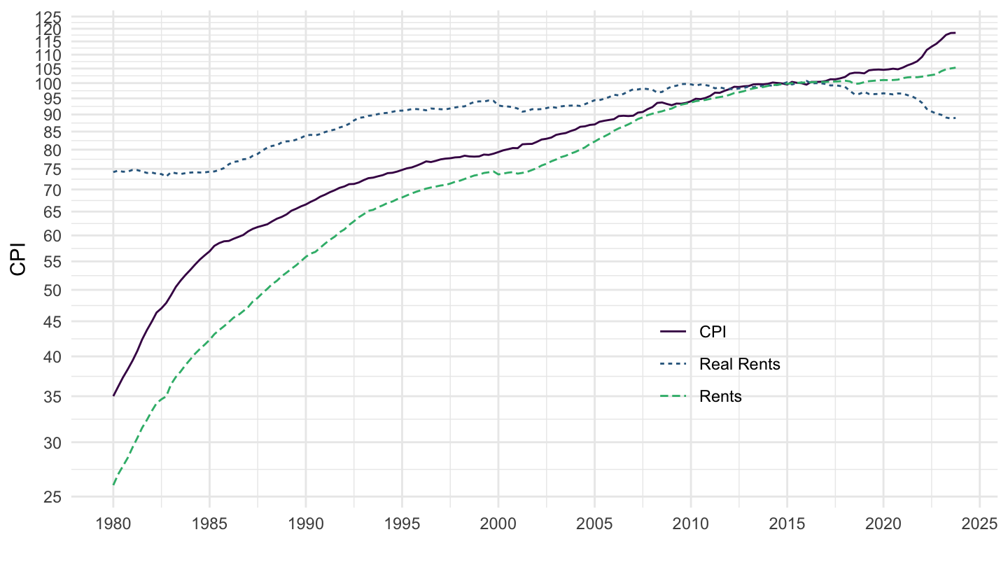
PRICES_CPI |>
  filter(LOCATION %in% c("FRA"),
         SUBJECT %in% c("CP040100", "CPALTT01"),
         FREQUENCY == "Q",
         MEASURE == "IXOB") |>
  quarter_to_date() |>
  filter(date >= as.Date("2000-01-01")) |>
  select(SUBJECT, date, LOCATION, obsValue) |>
  spread(SUBJECT, obsValue) |>
  filter(!is.na(CP040100)) |>
  mutate(rents_real = 100*CP040100/CPALTT01) |>
  select(date, LOCATION, CPALTT01, rents_real, CP040100) |>
  gather(variable, value, - date, -LOCATION) |>
  mutate(Variable = case_when(variable == "rents_real" ~ "Real Rents",
                              variable == "CP040100" ~ "Rents",
                              variable == "CPALTT01" ~ "CPI")) |>
  left_join(PRICES_CPI_var$LOCATION, by = "LOCATION") |>
  ggplot() + theme_minimal() + xlab("") + ylab("CPI") +
  geom_line(aes(x = date, y = value, color = Variable, linetype = Variable)) +
  scale_x_date(breaks = seq(1960, 2100, 2) |> paste0("-01-01") |> as.Date(),
               labels = date_format("%Y")) +
  scale_y_log10(breaks = seq(0, 200, 5)) +
  scale_color_manual(values = viridis(4)[1:3]) +
  theme(legend.position = c(0.7, 0.30),
        legend.title = element_blank())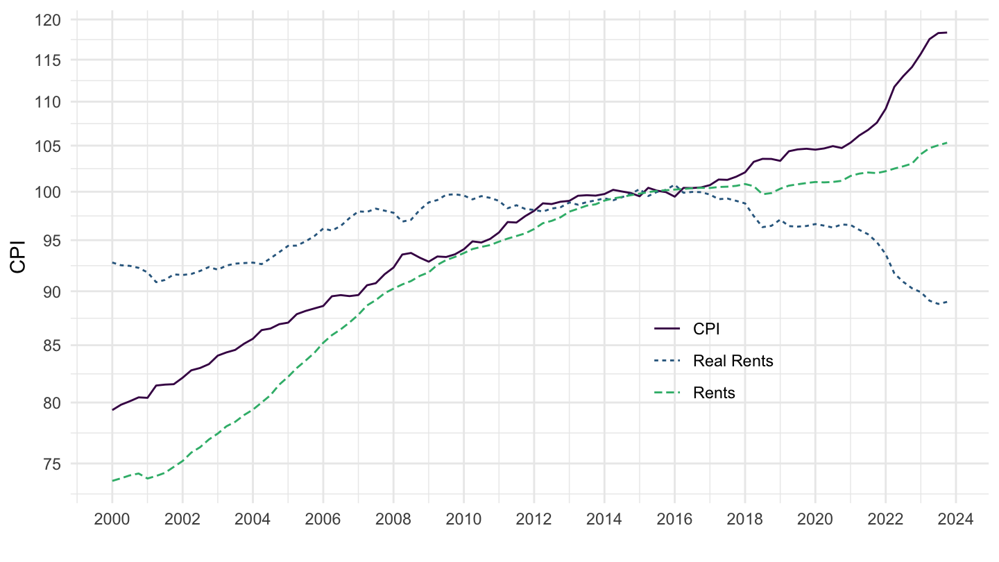
PRICES_CPI |>
  filter(LOCATION %in% c("FRA"),
         SUBJECT %in% c("CP040100", "CPALTT01"),
         FREQUENCY == "Q",
         MEASURE == "IXOB") |>
  quarter_to_date() |>
  filter(date >= as.Date("2010-01-01")) |>
  select(SUBJECT, date, LOCATION, obsValue) |>
  spread(SUBJECT, obsValue) |>
  filter(!is.na(CP040100)) |>
  mutate(rents_real = 100*CP040100/CPALTT01) |>
  select(date, LOCATION, CPALTT01, rents_real, CP040100) |>
  gather(variable, value, - date, -LOCATION) |>
  mutate(Variable = case_when(variable == "rents_real" ~ "Real Rents",
                              variable == "CP040100" ~ "Rents",
                              variable == "CPALTT01" ~ "CPI")) |>
  left_join(PRICES_CPI_var$LOCATION, by = "LOCATION") |>
  ggplot() + theme_minimal() + xlab("") + ylab("CPI") +
  geom_line(aes(x = date, y = value, color = Variable, linetype = Variable)) +
  scale_x_date(breaks = seq(1960, 2100, 1) |> paste0("-01-01") |> as.Date(),
               labels = date_format("%Y")) +
  scale_y_log10(breaks = seq(0, 200, 1)) +
  scale_color_manual(values = viridis(4)[1:3]) +
  theme(legend.position = c(0.7, 0.30),
        legend.title = element_blank())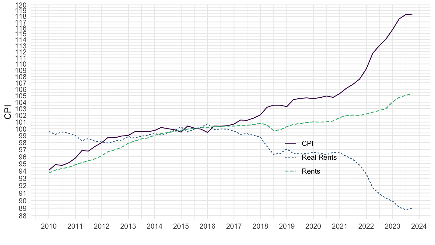
PRICES_CPI |>
  filter(LOCATION %in% c("AUS"),
         SUBJECT %in% c("CP040100", "CPALTT01"),
         FREQUENCY == "Q",
         MEASURE == "IXOB") |>
  quarter_to_date() |>
  filter(date >= as.Date("1980-01-01")) |>
  select(SUBJECT, date, LOCATION, obsValue) |>
  spread(SUBJECT, obsValue) |>
  filter(!is.na(CP040100)) |>
  mutate(rents_real = 100*CP040100/CPALTT01) |>
  select(date, LOCATION, CPALTT01, rents_real, CP040100) |>
  gather(variable, value, - date, -LOCATION) |>
  mutate(Variable = case_when(variable == "rents_real" ~ "Real Rents",
                              variable == "CP040100" ~ "Rents",
                              variable == "CPALTT01" ~ "CPI")) |>
  left_join(PRICES_CPI_var$LOCATION, by = "LOCATION") |>
  ggplot() + theme_minimal() + xlab("") + ylab("CPI") +
  geom_line(aes(x = date, y = value, color = Variable, linetype = Variable)) +
  scale_x_date(breaks = seq(1960, 2100, 5) |> paste0("-01-01") |> as.Date(),
               labels = date_format("%Y")) +
  scale_y_log10(breaks = seq(0, 200, 5)) +
  scale_color_manual(values = viridis(4)[1:3]) +
  theme(legend.position = c(0.7, 0.30),
        legend.title = element_blank())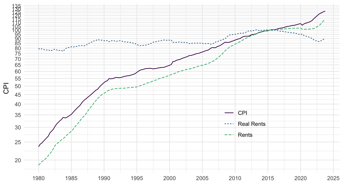
PRICES_CPI |>
  filter(LOCATION %in% c("AUS"),
         SUBJECT %in% c("CP040100", "CPALTT01"),
         FREQUENCY == "Q",
         MEASURE == "IXOB") |>
  quarter_to_date() |>
  filter(date >= as.Date("2000-01-01")) |>
  select(SUBJECT, date, LOCATION, obsValue) |>
  spread(SUBJECT, obsValue) |>
  filter(!is.na(CP040100)) |>
  mutate(rents_real = 100*CP040100/CPALTT01) |>
  select(date, LOCATION, CPALTT01, rents_real, CP040100) |>
  gather(variable, value, - date, -LOCATION) |>
  mutate(Variable = case_when(variable == "rents_real" ~ "Real Rents",
                              variable == "CP040100" ~ "Rents",
                              variable == "CPALTT01" ~ "CPI")) |>
  left_join(PRICES_CPI_var$LOCATION, by = "LOCATION") |>
  ggplot() + theme_minimal() + xlab("") + ylab("CPI") +
  geom_line(aes(x = date, y = value, color = Variable, linetype = Variable)) +
  scale_x_date(breaks = seq(1960, 2100, 2) |> paste0("-01-01") |> as.Date(),
               labels = date_format("%Y")) +
  scale_y_log10(breaks = seq(0, 200, 5)) +
  scale_color_manual(values = viridis(4)[1:3]) +
  theme(legend.position = c(0.7, 0.30),
        legend.title = element_blank())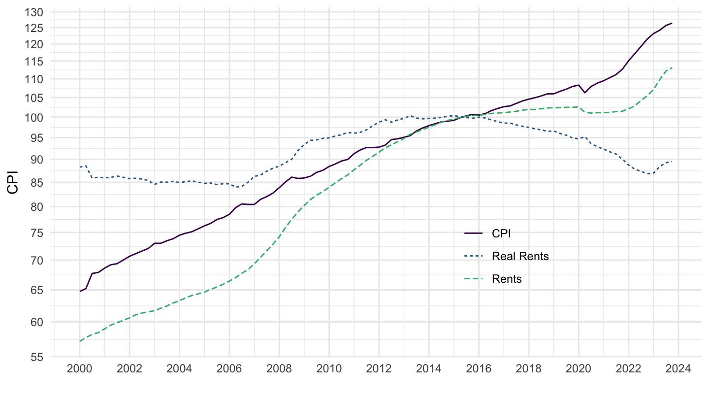
PRICES_CPI |>
  filter(LOCATION %in% c("AUS"),
         SUBJECT %in% c("CP040100", "CPALTT01"),
         FREQUENCY == "Q",
         MEASURE == "IXOB") |>
  quarter_to_date() |>
  filter(date >= as.Date("2010-01-01")) |>
  select(SUBJECT, date, LOCATION, obsValue) |>
  spread(SUBJECT, obsValue) |>
  filter(!is.na(CP040100)) |>
  mutate(rents_real = 100*CP040100/CPALTT01) |>
  select(date, LOCATION, CPALTT01, rents_real, CP040100) |>
  gather(variable, value, - date, -LOCATION) |>
  mutate(Variable = case_when(variable == "rents_real" ~ "Real Rents",
                              variable == "CP040100" ~ "Rents",
                              variable == "CPALTT01" ~ "CPI")) |>
  left_join(PRICES_CPI_var$LOCATION, by = "LOCATION") |>
  ggplot() + theme_minimal() + xlab("") + ylab("CPI") +
  geom_line(aes(x = date, y = value, color = Variable, linetype = Variable)) +
  scale_x_date(breaks = seq(1960, 2100, 1) |> paste0("-01-01") |> as.Date(),
               labels = date_format("%Y")) +
  scale_y_log10(breaks = seq(0, 200, 1)) +
  scale_color_manual(values = viridis(4)[1:3]) +
  theme(legend.position = c(0.7, 0.30),
        legend.title = element_blank())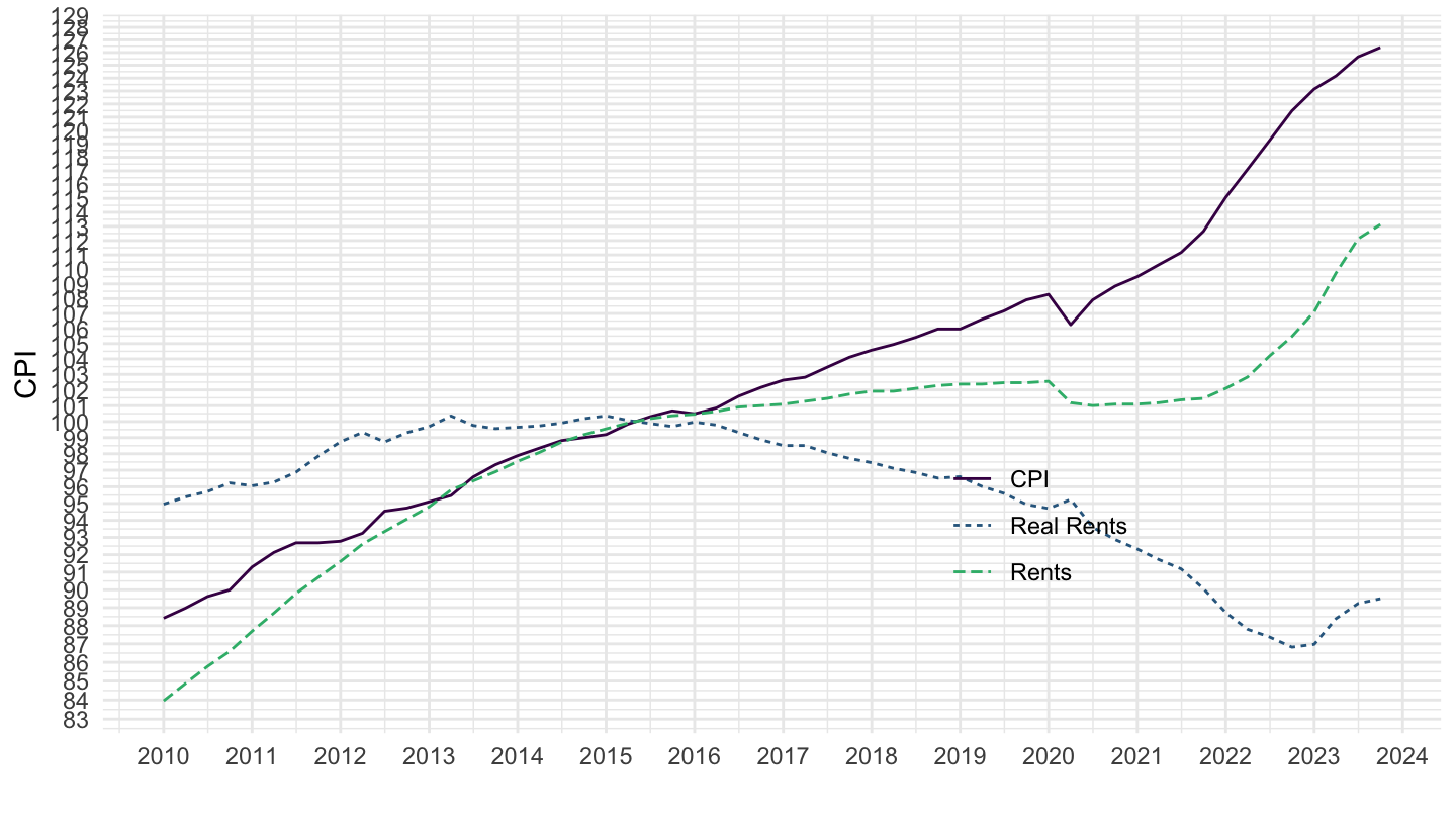
PRICES_CPI |>
  filter(LOCATION %in% c("FRA", "USA", "DEU", "JPN"),
         SUBJECT %in% c("CP040100", "CPALTT01"),
         FREQUENCY == "Q",
         MEASURE == "IXOB") |>
  quarter_to_date() |>
  select(SUBJECT, date, LOCATION, obsValue) |>
  spread(SUBJECT, obsValue) |>
  filter(!is.na(CP040100)) |>
  mutate(obsValue = 100*CP040100/CPALTT01) |>
  group_by(LOCATION) |>
  left_join(PRICES_CPI_var$LOCATION, by = "LOCATION") |>
  add_flag_color("Location") |>
  ggplot() + geom_line(aes(x = date, y = obsValue, color = color)) +
  scale_color_identity() + add_4flags +
  theme_minimal() + xlab("") + ylab("CPI, Real Actual rentals for housing") +
  scale_x_date(breaks = seq(1960, 2100, 5) |> paste0("-01-01") |> as.Date(),
               labels = date_format("%Y")) +
  scale_y_log10(breaks = seq(0, 200, 10)) +
  theme(legend.position = c(0.7, 0.30),
        legend.title = element_blank())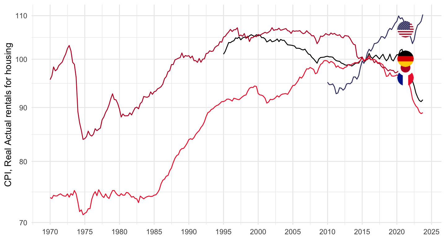
PRICES_CPI |>
  filter(LOCATION %in% c("FRA", "USA", "DEU", "JPN"),
         SUBJECT %in% c("CP040100", "CPALTT01"),
         FREQUENCY == "Q",
         MEASURE == "IXOB") |>
  quarter_to_date() |>
  filter(date >= as.Date("1990-01-01")) |>
  select(SUBJECT, date, LOCATION, obsValue) |>
  spread(SUBJECT, obsValue) |>
  filter(!is.na(CP040100)) |>
  mutate(obsValue = 100*CP040100/CPALTT01) |>
  group_by(LOCATION) |>
  left_join(PRICES_CPI_var$LOCATION, by = "LOCATION") |>
  add_flag_color("Location") |>
  ggplot() + geom_line(aes(x = date, y = obsValue, color = color)) +
  scale_color_identity() + add_4flags +
  theme_minimal() + xlab("") + ylab("CPI, Real Actual rentals for housing") +
  scale_x_date(breaks = seq(1960, 2100, 5) |> paste0("-01-01") |> as.Date(),
               labels = date_format("%Y")) +
  scale_y_log10(breaks = seq(0, 200, 10)) +
  theme(legend.position = c(0.7, 0.30),
        legend.title = element_blank())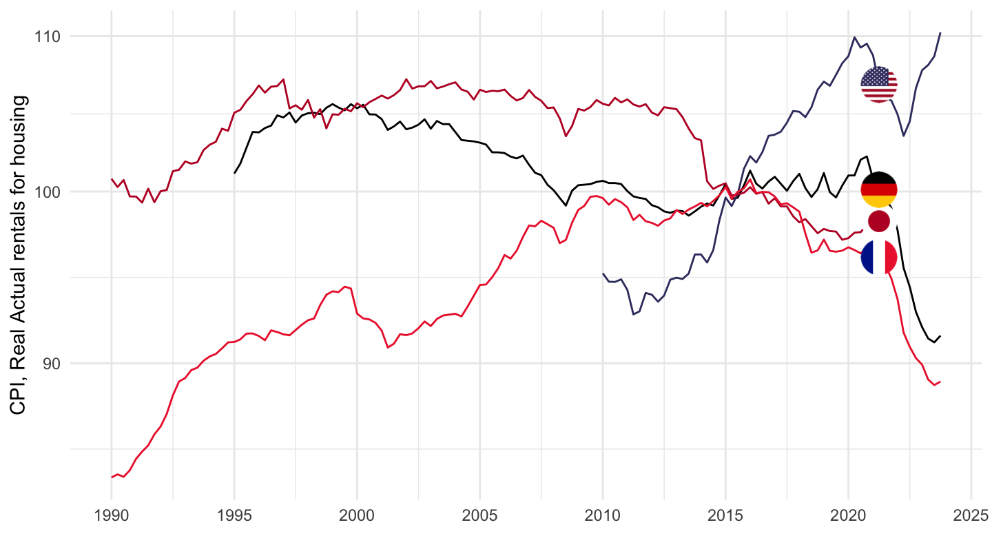
PRICES_CPI |>
  filter(LOCATION %in% c("FRA", "USA", "DEU", "JPN"),
         SUBJECT %in% c("CP040100", "CPALTT01"),
         FREQUENCY == "Q",
         MEASURE == "IXOB") |>
  quarter_to_date() |>
  filter(date >= as.Date("2000-01-01")) |>
  select(SUBJECT, date, LOCATION, obsValue) |>
  spread(SUBJECT, obsValue) |>
  filter(!is.na(CP040100)) |>
  mutate(obsValue = 100*CP040100/CPALTT01) |>
  group_by(LOCATION) |>
  left_join(PRICES_CPI_var$LOCATION, by = "LOCATION") |>
  add_flag_color("Location") |>
  ggplot() + geom_line(aes(x = date, y = obsValue, color = color)) +
  scale_color_identity() + add_4flags +
  theme_minimal() + xlab("") + ylab("CPI, Real Actual rentals for housing") +
  scale_x_date(breaks = seq(1960, 2100, 2) |> paste0("-01-01") |> as.Date(),
               labels = date_format("%Y")) +
  scale_y_log10(breaks = seq(0, 200, 1)) +
  theme(legend.position = c(0.15, 0.5),
        legend.title = element_blank())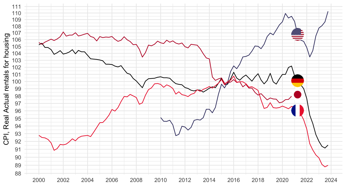
PRICES_CPI |>
  filter(LOCATION %in% c("KOR", "CAN", "PRT", "ESP"),
         SUBJECT %in% c("CP040100", "CPALTT01"),
         FREQUENCY == "Q",
         MEASURE == "IXOB") |>
  quarter_to_date() |>
  select(SUBJECT, date, LOCATION, obsValue) |>
  spread(SUBJECT, obsValue) |>
  filter(!is.na(CP040100)) |>
  mutate(obsValue = 100*CP040100/CPALTT01) |>
  group_by(LOCATION) |>
  left_join(PRICES_CPI_var$LOCATION, by = "LOCATION") |>
  add_flag_color("Location") |>
  ggplot() + geom_line(aes(x = date, y = obsValue, color = color)) +
  scale_color_identity() + add_4flags +
  theme_minimal() + xlab("") + ylab("CPI, Real Actual rentals for housing") +
  scale_x_date(breaks = seq(1960, 2100, 5) |> paste0("-01-01") |> as.Date(),
               labels = date_format("%Y")) +
  scale_y_log10(breaks = seq(0, 200, 10)) +
  theme(legend.position = c(0.7, 0.80),
        legend.title = element_blank())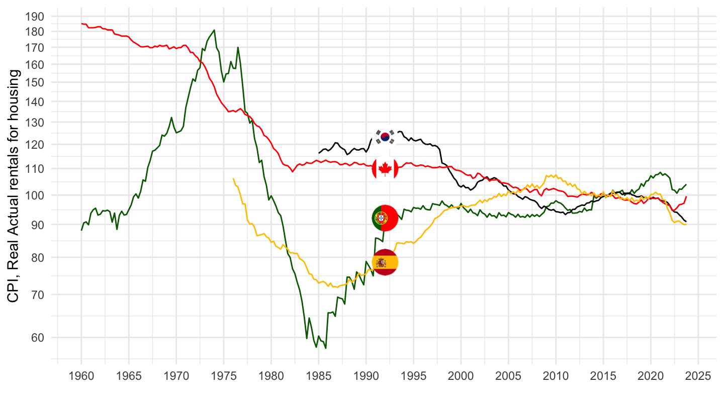
PRICES_CPI |>
  filter(LOCATION %in% c("DNK", "AUS", "AUT", "BEL"),
         SUBJECT %in% c("CP040100", "CPALTT01"),
         FREQUENCY == "Q",
         MEASURE == "IXOB") |>
  quarter_to_date() |>
  select(SUBJECT, date, LOCATION, obsValue) |>
  spread(SUBJECT, obsValue) |>
  filter(!is.na(CP040100)) |>
  mutate(obsValue = 100*CP040100/CPALTT01) |>
  group_by(LOCATION) |>
  left_join(PRICES_CPI_var$LOCATION, by = "LOCATION") |>
  add_flag_color("Location") |>
  ggplot() + geom_line(aes(x = date, y = obsValue, color = color)) +
  scale_color_identity() + add_4flags +
  theme_minimal() + xlab("") + ylab("CPI, Real Actual rentals for housing") +
  scale_x_date(breaks = seq(1960, 2100, 5) |> paste0("-01-01") |> as.Date(),
               labels = date_format("%Y")) +
  scale_y_log10(breaks = seq(0, 200, 5)) +
  theme(legend.position = c(0.2, 0.80),
        legend.title = element_blank())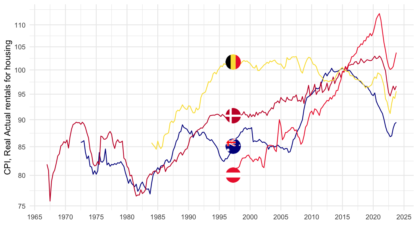
PRICES_CPI_CPALTT01_IXOB <- PRICES_CPI |>
  filter(SUBJECT == "CPALTT01",
         FREQUENCY == "Q",
         MEASURE == "IXOB") |>
  left_join(PRICES_CPI_var$LOCATION, by = "LOCATION") |>
  select(LOCATION, Location, obsTime, CPALTT01_IXOB = obsValue)

save(PRICES_CPI_CPALTT01_IXOB, file = "PRICES_CPI_CPALTT01_IXOB_2.RData")

PRICES_CPI_CPALTT01_IXOB <- PRICES_CPI |>
  filter(SUBJECT == "CPALTT01",
         FREQUENCY == "Q",
         MEASURE == "IXOB") |>
  quarter_to_date() |>
  left_join(PRICES_CPI_var$LOCATION, by = "LOCATION") |>
  select(LOCATION, Location, date, CPALTT01_IXOB = obsValue)

save(PRICES_CPI_CPALTT01_IXOB, file = "PRICES_CPI_CPALTT01_IXOB.RData")

PRICES_CPI_CPALTT01_IXOB |>
  filter(LOCATION %in% c("FRA", "USA", "DEU", "JPN")) |>
  add_flag_color("Location") |>
  rename(obsValue = CPALTT01_IXOB) |>
  ggplot() + geom_line(aes(x = date, y = obsValue, color = color)) +
  scale_color_identity() + add_4flags + theme_minimal() +
  scale_x_date(breaks = seq(1960, 2100, 5) |> paste0("-01-01") |> as.Date(),
               labels = date_format("%Y")) +
  scale_y_log10(breaks = seq(0, 200, 10)) +
  theme(legend.position = c(0.7, 0.30),
        legend.title = element_blank())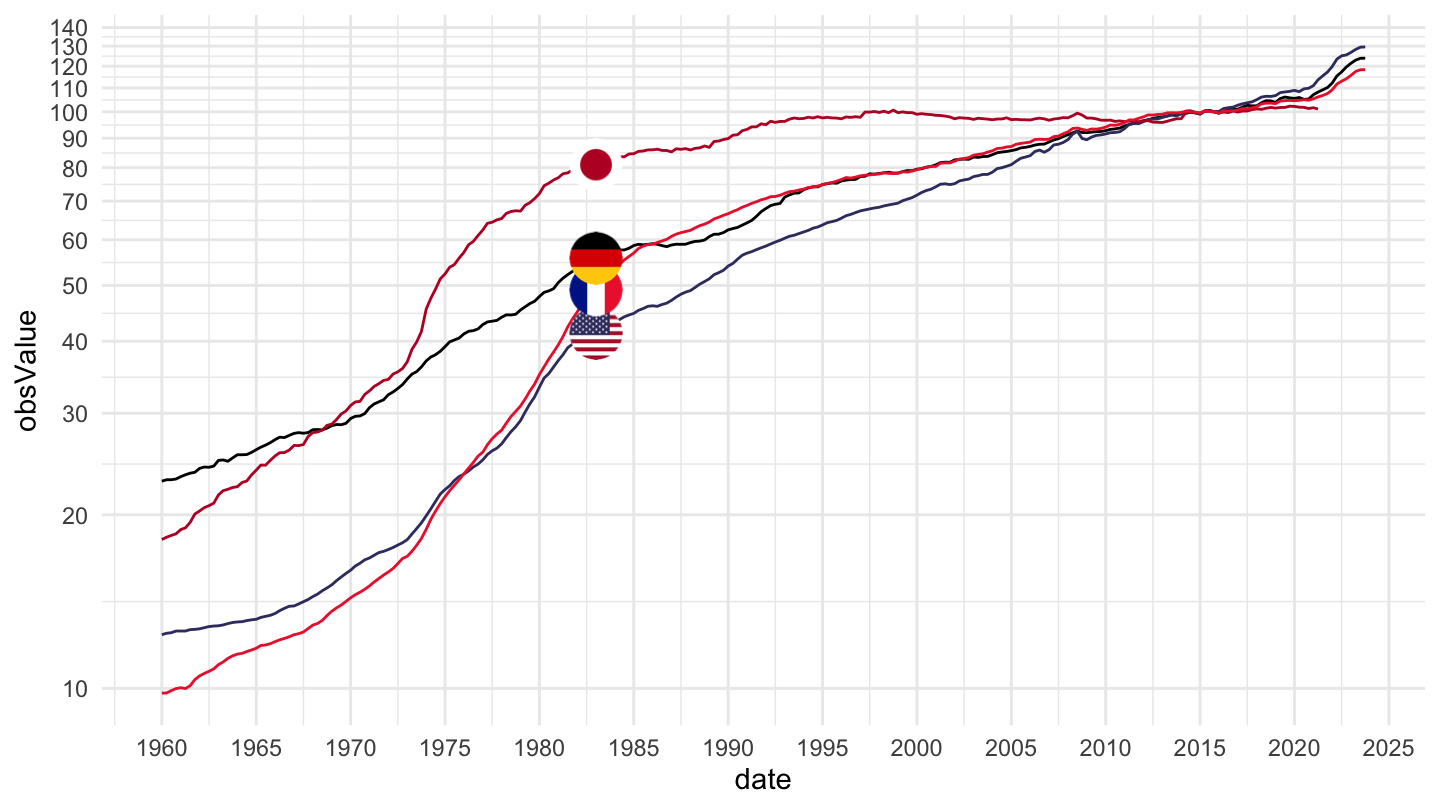
PRICES_CPI_CPALTT01_IXOB |>
  filter(LOCATION %in% c("FRA", "USA", "DEU", "JPN"),
         date >= as.Date("1990-01-01")) |>
  add_flag_color("Location") |>
  rename(obsValue = CPALTT01_IXOB) |>
  group_by(Location) |>
  mutate(obsValue = 100*obsValue/obsValue[1]) |>
  ggplot() + geom_line(aes(x = date, y = obsValue, color = color)) +
  scale_color_identity() + add_4flags + theme_minimal() + xlab("") + ylab("") +
  scale_x_date(breaks = seq(1960, 2100, 5) |> paste0("-01-01") |> as.Date(),
               labels = date_format("%Y")) +
  scale_y_log10(breaks = seq(0, 400, 10)) +
  theme(legend.position = c(0.7, 0.30),
        legend.title = element_blank())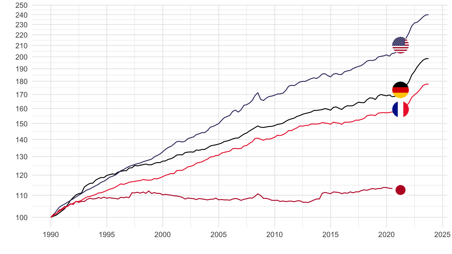
PRICES_CPI_CPALTT01_IXOB |>
  filter(LOCATION %in% c("FRA", "USA", "DEU", "JPN"),
         date >= as.Date("1996-01-01")) |>
  add_flag_color("Location") |>
  rename(obsValue = CPALTT01_IXOB) |>
  group_by(Location) |>
  mutate(obsValue = 100*obsValue/obsValue[1]) |>
  ggplot() + geom_line(aes(x = date, y = obsValue, color = color)) +
  scale_color_identity() + add_4flags + theme_minimal() + xlab("") + ylab("") +
  scale_x_date(breaks = seq(1960, 2100, 2) |> paste0("-01-01") |> as.Date(),
               labels = date_format("%Y")) +
  scale_y_log10(breaks = seq(0, 400, 10)) +
  theme(legend.position = c(0.7, 0.30),
        legend.title = element_blank())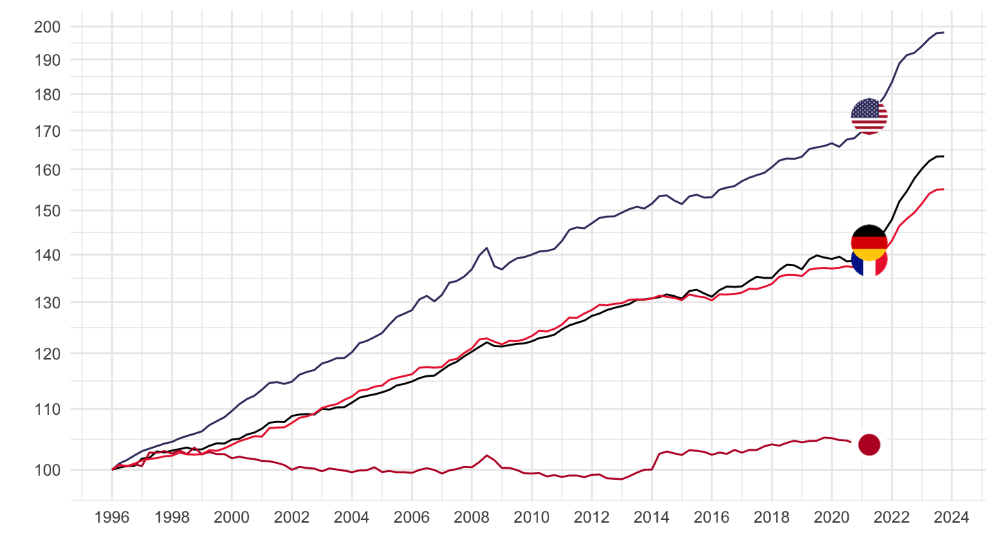
PRICES_CPI |>
  filter(LOCATION %in% c("FRA", "USA", "DEU", "JPN"),
         SUBJECT == "CPGRLH01",
         FREQUENCY == "Q",
         MEASURE == "IXOB") |>
  quarter_to_date() |>
  left_join(PRICES_CPI_var$LOCATION, by = "LOCATION") |>
  add_flag_color("Location") |>
  ggplot() + geom_line(aes(x = date, y = obsValue, color = color)) +
  scale_color_identity() + add_2flags + theme_minimal() +
  theme_minimal() + xlab("") + ylab("Services less housing") +
  scale_x_date(breaks = seq(1960, 2100, 5) |> paste0("-01-01") |> as.Date(),
               labels = date_format("%Y")) +
  scale_y_log10(breaks = seq(0, 200, 10))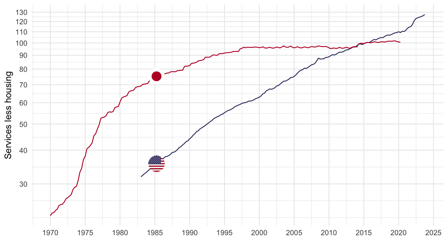
PRICES_CPI |>
  filter(LOCATION %in% c("FRA", "USA", "DEU", "JPN"),
         SUBJECT == "CP010000",
         FREQUENCY == "Q",
         MEASURE == "IXOB") |>
  quarter_to_date() |>
  left_join(PRICES_CPI_var$LOCATION, by = "LOCATION") |>
  add_flag_color("Location") |>
  ggplot() + geom_line(aes(x = date, y = obsValue, color = color)) +
  scale_color_identity() + add_4flags +
  theme_minimal() + xlab("") + ylab("CPI, Food and non-Alcoholic beverages") +
  scale_x_date(breaks = seq(1960, 2100, 5) |> paste0("-01-01") |> as.Date(),
               labels = date_format("%Y")) +
  scale_y_log10(breaks = seq(0, 200, 10))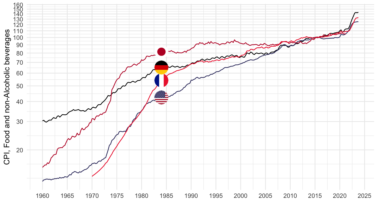
PRICES_CPI |>
  filter(LOCATION %in% c("FRA", "USA", "DEU", "JPN"),
         SUBJECT == "CP030000",
         FREQUENCY == "Q",
         MEASURE == "IXOB") |>
  quarter_to_date() |>
  left_join(PRICES_CPI_var$LOCATION, by = "LOCATION") |>
  add_flag_color("Location") |>
  ggplot() + geom_line(aes(x = date, y = obsValue, color = color)) +
  scale_color_identity() + add_4flags + theme_minimal() +
  theme_minimal() + xlab("") + ylab("CPI, Clothing and Footware") +
  scale_x_date(breaks = seq(1960, 2100, 5) |> paste0("-01-01") |> as.Date(),
               labels = date_format("%Y")) +
  scale_y_log10(breaks = seq(0, 200, 10))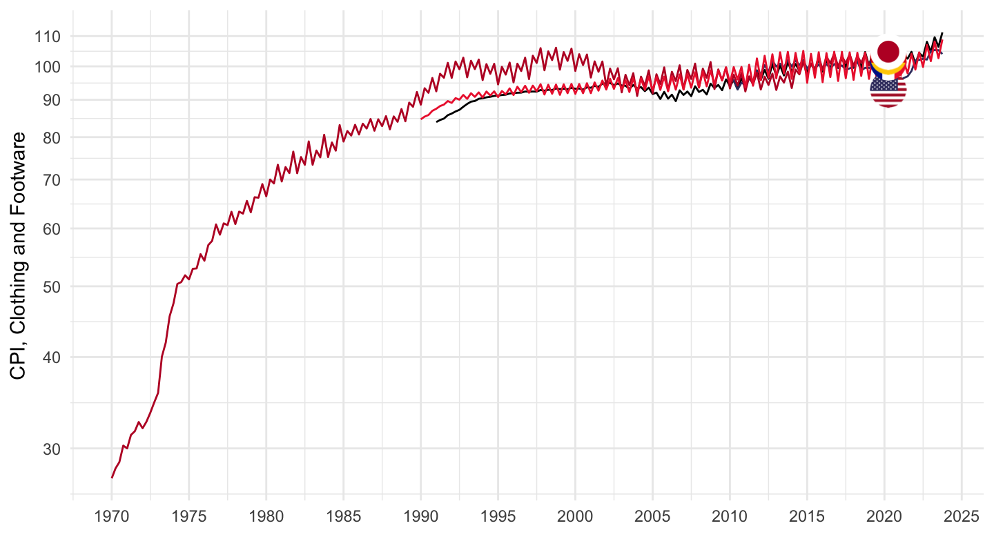
PRICES_CPI |>
  filter(LOCATION %in% c("FRA", "USA", "DEU", "JPN"),
         SUBJECT == "CP110000",
         FREQUENCY == "Q",
         MEASURE == "IXOB") |>
  quarter_to_date() |>
  left_join(PRICES_CPI_var$LOCATION, by = "LOCATION") |>
  add_flag_color("Location") |>
  ggplot() + geom_line(aes(x = date, y = obsValue, color = color)) +
  scale_color_identity() + add_4flags + theme_minimal() +
  theme_minimal() + xlab("") + ylab("CPI,  Restaurants and hotels") +
  scale_x_date(breaks = seq(1960, 2100, 5) |> paste0("-01-01") |> as.Date(),
               labels = date_format("%Y")) +
  scale_y_log10(breaks = seq(0, 200, 10))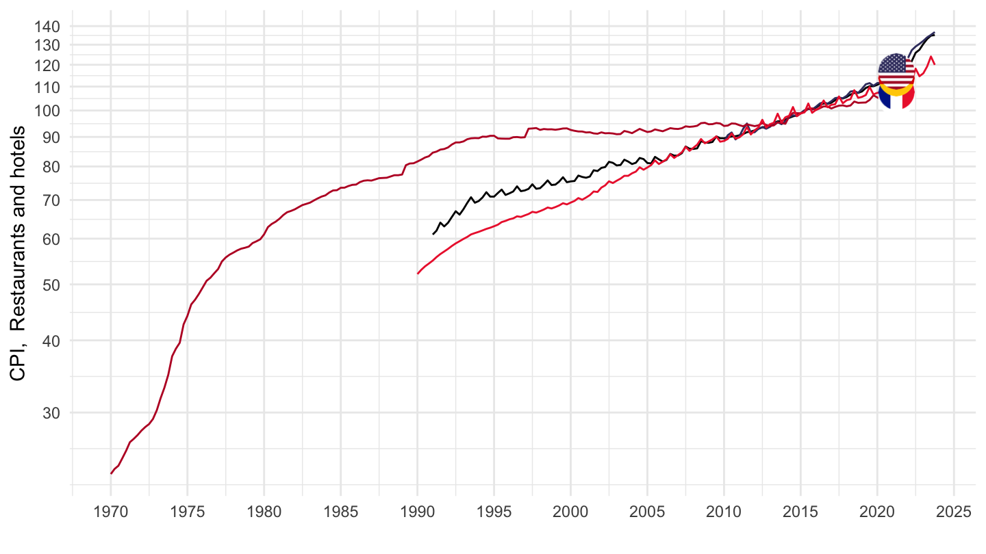
PRICES_CPI |>
  filter(LOCATION %in% c("FRA", "USA", "DEU", "JPN"),
         SUBJECT == "CP040100",
         FREQUENCY == "Q",
         MEASURE == "IXOB") |>
  quarter_to_date() |>
  left_join(PRICES_CPI_var$LOCATION, by = "LOCATION") |>
  add_flag_color("Location") |>
  ggplot() + geom_line(aes(x = date, y = obsValue, color = color)) +
  scale_color_identity() + add_4flags + theme_minimal() +
  theme_minimal() + xlab("") + ylab("CPI, Actual rentals for housing") +
  scale_x_date(breaks = seq(1960, 2100, 5) |> paste0("-01-01") |> as.Date(),
               labels = date_format("%Y")) +
  scale_y_log10(breaks = seq(0, 200, 10))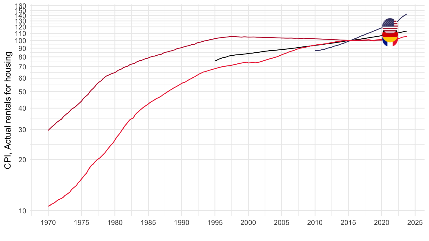
PRICES_CPI |>
  filter(LOCATION %in% c("FRA", "DEU"),
         SUBJECT %in% c("CPALTT01"),
         FREQUENCY == "M",
         MEASURE == "IXOB") |>
  left_join(PRICES_CPI_var$LOCATION, by = "LOCATION") |>
  month_to_date() |>
  filter(date >= as.Date("1990-01-01")) |>
  add_flag_color("Location") |>
  group_by(Location) |>
  mutate(obsValue = 100*obsValue/obsValue[1]) |>
  ggplot() + geom_line(aes(x = date, y = obsValue, color = color)) +
  scale_color_identity() + add_2flags + theme_minimal() + xlab("") + ylab("") +
  scale_x_date(breaks = seq(1960, 2100, 2) |> paste0("-01-01") |> as.Date(),
               labels = date_format("%Y")) +
  scale_y_log10(breaks = seq(0, 400, 10)) +
  theme(legend.position = c(0.7, 0.30),
        legend.title = element_blank())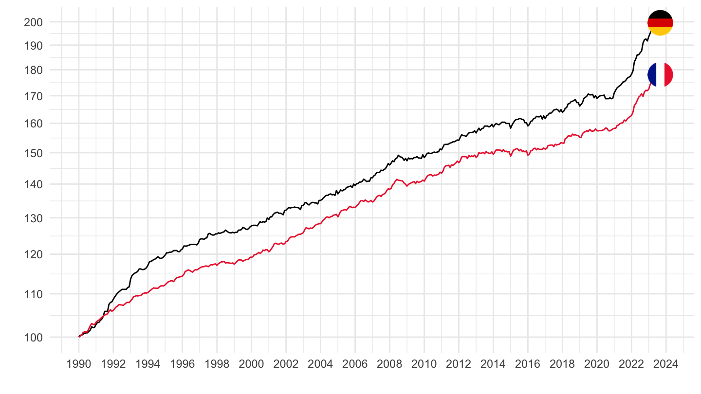
PRICES_CPI |>
  filter(LOCATION %in% c("FRA", "DEU"),
         SUBJECT %in% c("CPALTT01"),
         FREQUENCY == "M",
         MEASURE == "IXOB") |>
  left_join(PRICES_CPI_var$LOCATION, by = "LOCATION") |>
  month_to_date() |>
  filter(date >= as.Date("1996-01-01")) |>
  add_flag_color("Location") |>
  group_by(Location) |>
  mutate(obsValue = 100*obsValue/obsValue[1]) |>
  ggplot() + geom_line(aes(x = date, y = obsValue, color = color)) +
  scale_color_identity() + add_2flags + theme_minimal() + xlab("") + ylab("") +
  scale_x_date(breaks = seq(1960, 2100, 2) |> paste0("-01-01") |> as.Date(),
               labels = date_format("%Y")) +
  scale_y_log10(breaks = seq(0, 400, 10)) +
  theme(legend.position = c(0.7, 0.30),
        legend.title = element_blank())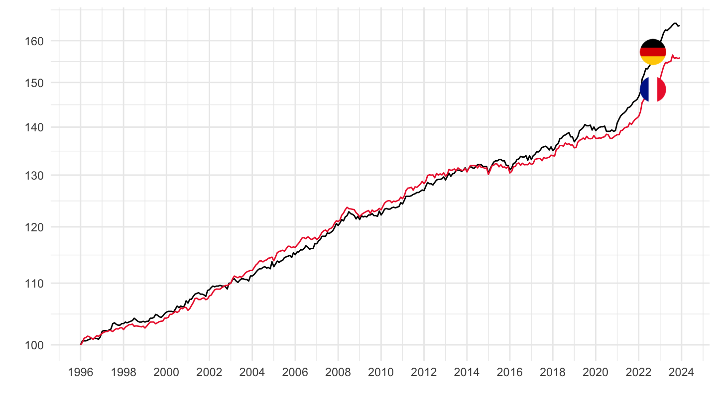
PRICES_CPI_CPALTT01_IXOB |>
  filter(LOCATION %in% c("FRA", "DEU"),
         date >= as.Date("1990-01-01")) |>
  add_flag_color("Location") |>
  rename(obsValue = CPALTT01_IXOB) |>
  group_by(Location) |>
  mutate(obsValue = 100*obsValue/obsValue[1]) |>
  ggplot() + geom_line(aes(x = date, y = obsValue, color = color)) +
  scale_color_identity() + add_2flags + theme_minimal() + xlab("") + ylab("") +
  scale_x_date(breaks = seq(1960, 2100, 5) |> paste0("-01-01") |> as.Date(),
               labels = date_format("%Y")) +
  scale_y_log10(breaks = seq(0, 400, 10)) +
  theme(legend.position = c(0.7, 0.30),
        legend.title = element_blank())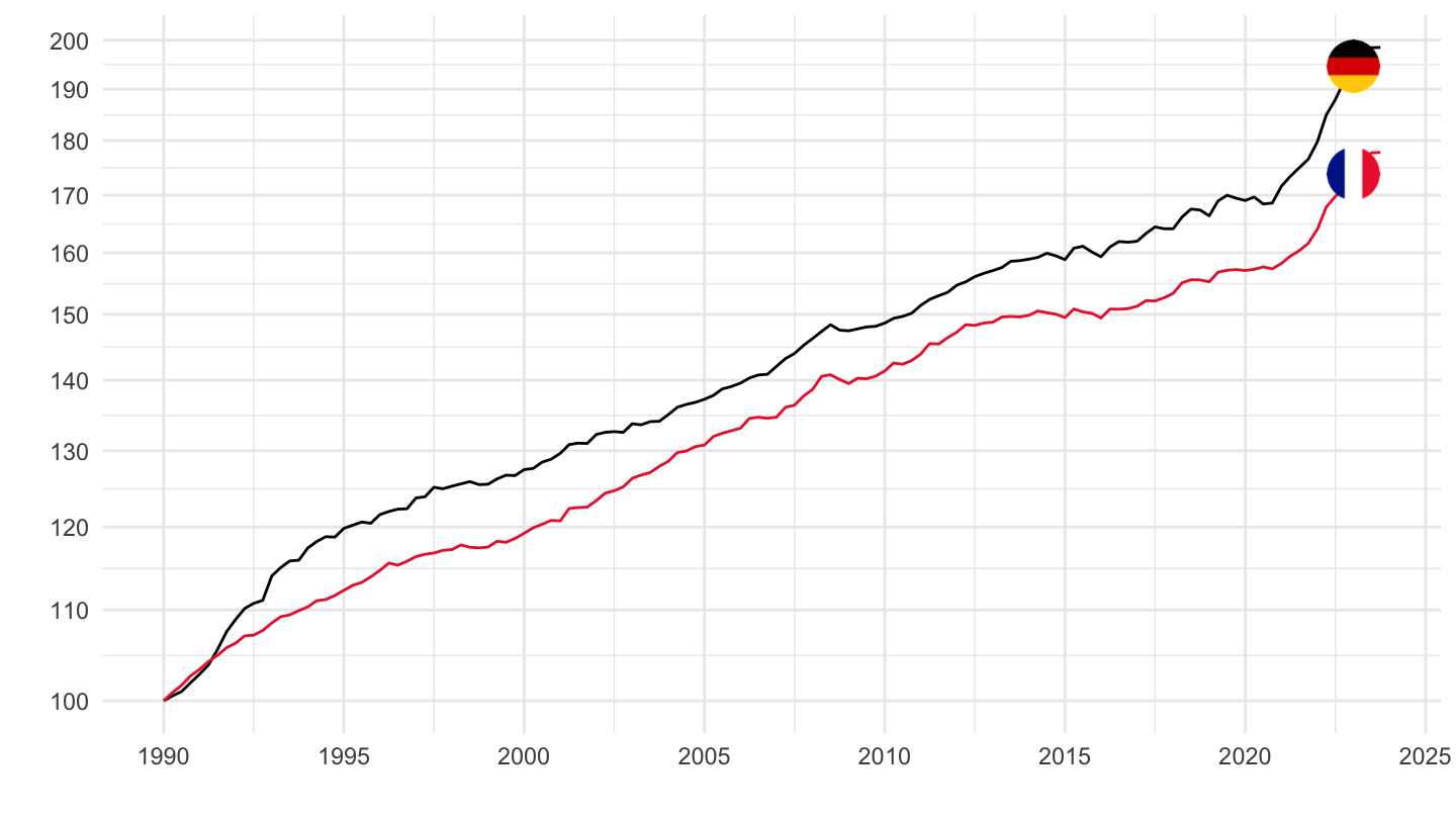
PRICES_CPI_CPALTT01_IXOB |>
  filter(LOCATION %in% c("FRA", "DEU"),
         date >= as.Date("1996-01-01")) |>
  add_flag_color("Location") |>
  rename(obsValue = CPALTT01_IXOB) |>
  group_by(Location) |>
  mutate(obsValue = 100*obsValue/obsValue[1]) |>
  ggplot() + geom_line(aes(x = date, y = obsValue, color = color)) +
  scale_color_identity() + add_2flags + theme_minimal() + xlab("") + ylab("") +
  scale_x_date(breaks = seq(1960, 2100, 2) |> paste0("-01-01") |> as.Date(),
               labels = date_format("%Y")) +
  scale_y_log10(breaks = seq(0, 400, 10)) +
  theme(legend.position = c(0.7, 0.30),
        legend.title = element_blank())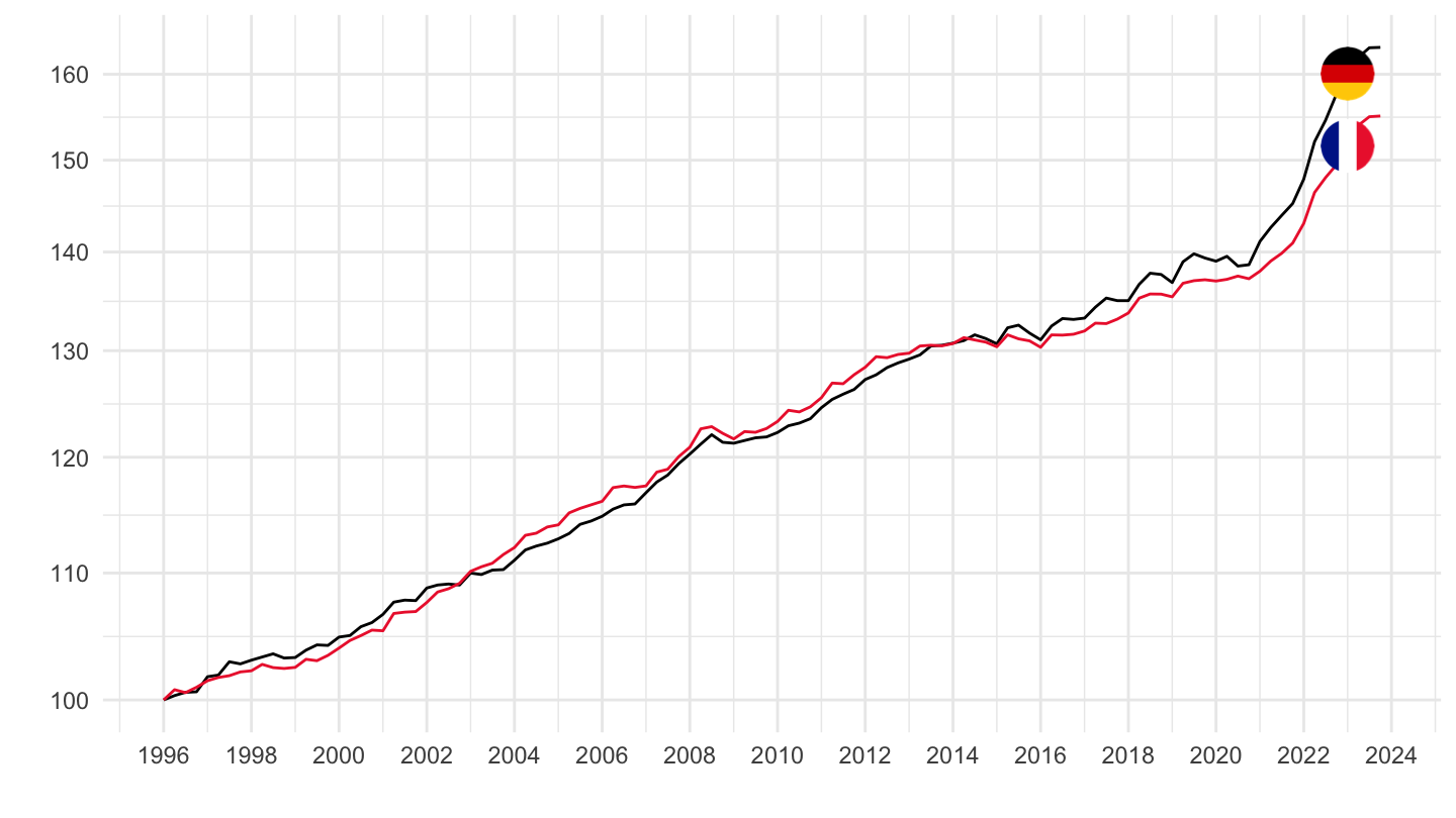
| source | dataset | Title | Updated |
|---|---|---|---|
| source | dataset | Title | Updated |
|---|---|---|---|
| source | dataset | Title | Updated |
|---|---|---|---|



