House price index (2015 = 100) - quarterly data
Data - Eurostat
Info
Last observation: Quarterly: 2026Q1 (N = 406)
First observation: Quarterly: 2005Q1 (N = 120)
Last data update: 23 jul 2026, 22:34. Last compile: 24 jul 2026, 03:45
Structure
Greece, Europe, France, Spain, Italy, Germany
Purchase Total
All
Code
prc_hpi_q %>%
  filter(purchase == "TOTAL",
         geo %in% c("EL", "FR", "ES", "IT", "DE"),
         unit == "I15_Q") %>%
  quarter_to_date %>%
  group_by(geo) %>%
  arrange(date) %>%
  mutate(values = 100*values/values[1]) %>%

  mutate(Geo = ifelse(geo == "EA", "Europe", Geo),
         Geo = ifelse(geo == "DE", "Germany", Geo)) %>%
  ggplot(.) + geom_line(aes(x = date, y = values, color = Geo)) +
  theme_minimal() + xlab("") + ylab("100 = Janv. 2006") +
  scale_x_date(breaks = seq(1960, 2100, 2) %>% paste0("-01-01") %>% as.Date,
               labels = date_format("%Y")) +
  scale_color_manual(values = c("#ED2939", "#000000", "#009246", "#FFC400")) +
  add_4flags +
  scale_y_log10(breaks = seq(0, 200, 5)) +
  theme(legend.position = "none",
        legend.title = element_blank())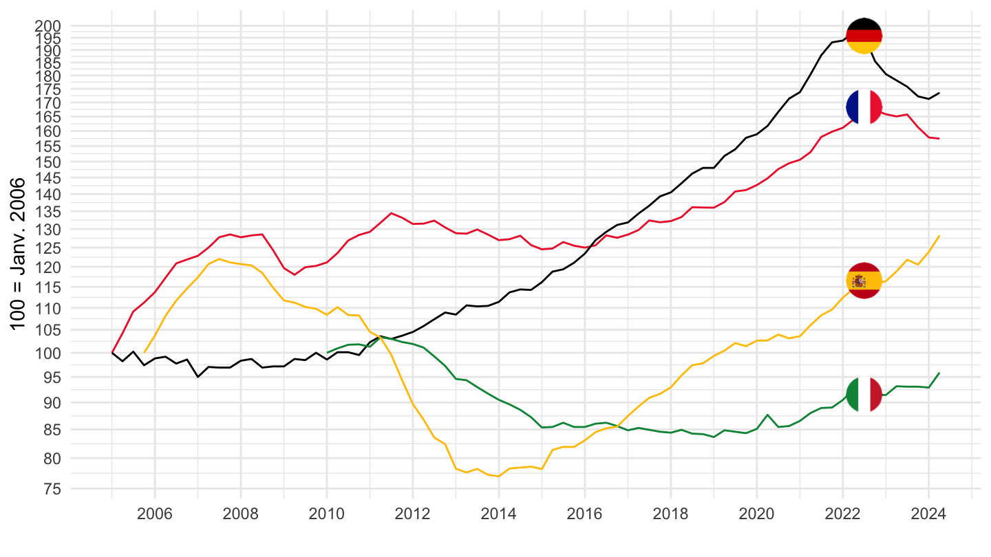
2009-2016
Code
prc_hpi_q %>%
  filter(purchase == "TOTAL",
         geo %in% c("EL", "FR", "ES", "IT", "DE"),
         unit == "I15_Q") %>%
  quarter_to_date %>%
  group_by(geo) %>%
  mutate(values = 100*values/values[date == as.Date("2011-01-01")]) %>%
  filter(date >= as.Date("2009-01-01"),
         date <= as.Date("2016-01-01")) %>%

  mutate(Geo = ifelse(geo == "EA", "Europe", Geo),
         Geo = ifelse(geo == "DE", "Germany", Geo)) %>%
  ggplot(.) + geom_line(aes(x = date, y = values, color = Geo)) +
  theme_minimal() + xlab("") + ylab("100 = Janv. 2011") +
  scale_x_date(breaks = seq(1960, 2100, 2) %>% paste0("-01-01") %>% as.Date,
               labels = date_format("%Y")) +
  scale_color_manual(values = c("#ED2939", "#000000", "#009246", "#FFC400")) +
  add_4flags +
  scale_y_log10(breaks = seq(0, 200, 5)) +
  theme(legend.position = "none",
        legend.title = element_blank())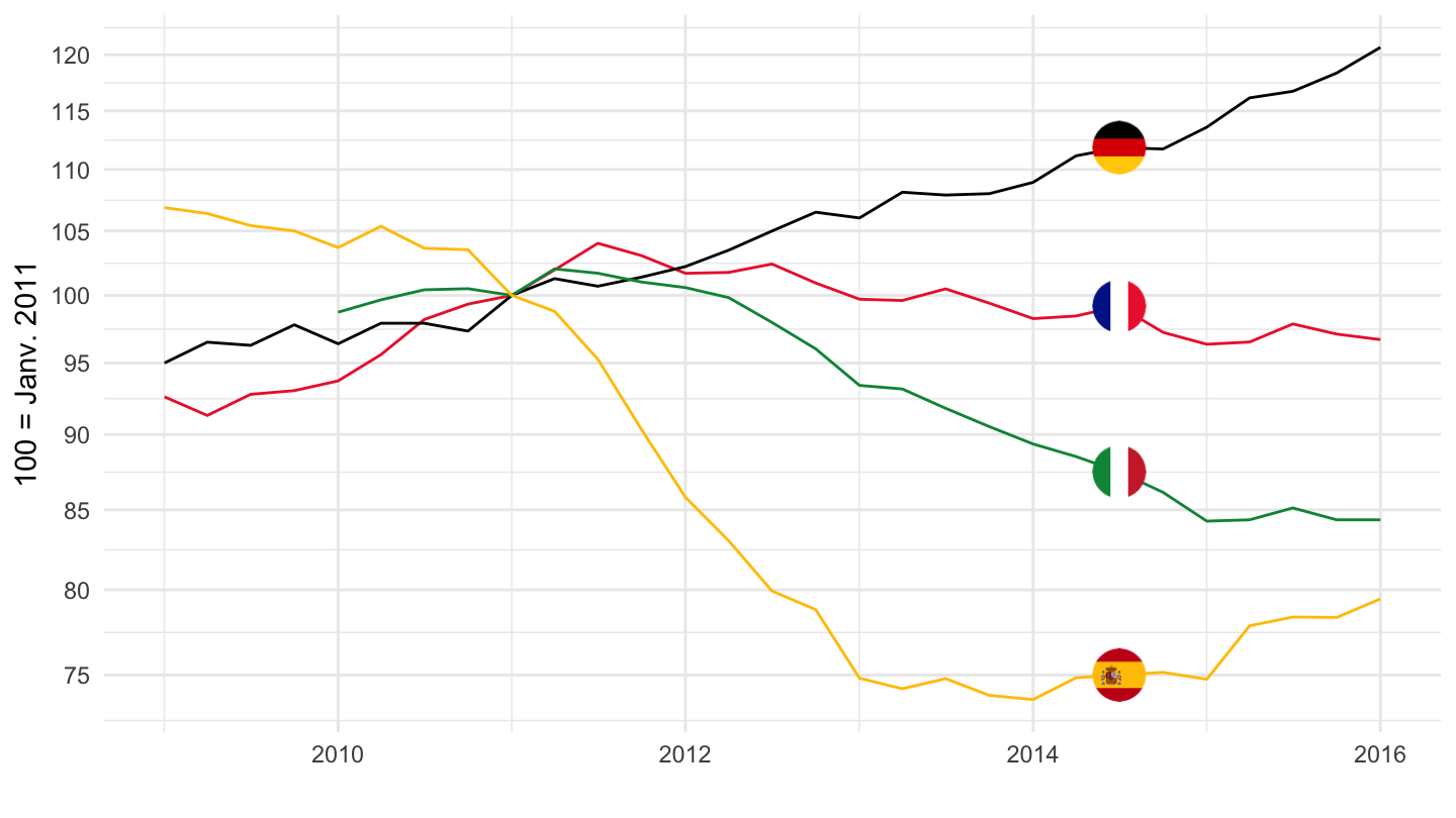
Existing Dwellings - DW_EXST
Code
prc_hpi_q %>%
  filter(purchase == "DW_EXST",
         geo %in% c("EL", "FR", "ES", "IT", "DE"),
         unit == "I15_Q") %>%
  quarter_to_date %>%
  group_by(geo) %>%
  mutate(values = 100*values/values[date == as.Date("2011-01-01")]) %>%
  filter(date >= as.Date("2009-01-01"),
         date <= as.Date("2016-01-01")) %>%

  mutate(Geo = ifelse(geo == "EA", "Europe", Geo),
         Geo = ifelse(geo == "DE", "Germany", Geo)) %>%
  ggplot(.) + geom_line(aes(x = date, y = values, color = Geo)) +
  theme_minimal() + xlab("") + ylab("100 = Janv. 2011") +
  scale_x_date(breaks = seq(1960, 2100, 2) %>% paste0("-01-01") %>% as.Date,
               labels = date_format("%Y")) +
  scale_color_manual(values = c("#ED2939", "#000000", "#009246", "#FFC400")) +
  add_4flags +
  scale_y_log10(breaks = seq(0, 200, 5)) +
  theme(legend.position = "none",
        legend.title = element_blank())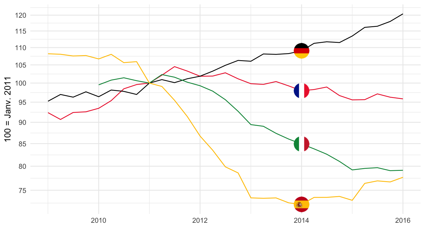
Purchases of new dwellings - DW_NEW
Code
prc_hpi_q %>%
  filter(purchase == "DW_NEW",
         geo %in% c("EL", "FR", "ES", "IT", "DE"),
         unit == "I15_Q") %>%
  quarter_to_date %>%
  group_by(geo) %>%
  mutate(values = 100*values/values[date == as.Date("2011-01-01")]) %>%
  filter(date >= as.Date("2009-01-01"),
         date <= as.Date("2016-01-01")) %>%

  mutate(Geo = ifelse(geo == "EA", "Europe", Geo),
         Geo = ifelse(geo == "DE", "Germany", Geo)) %>%
  ggplot(.) + geom_line(aes(x = date, y = values, color = Geo)) +
  theme_minimal() + xlab("") + ylab("100 = Janv. 2011") +
  scale_x_date(breaks = seq(1960, 2100, 2) %>% paste0("-01-01") %>% as.Date,
               labels = date_format("%Y")) +
  scale_color_manual(values = c("#ED2939", "#000000", "#009246", "#FFC400")) +
  add_4flags +
  scale_y_log10(breaks = seq(0, 200, 5)) +
  theme(legend.position = "none",
        legend.title = element_blank())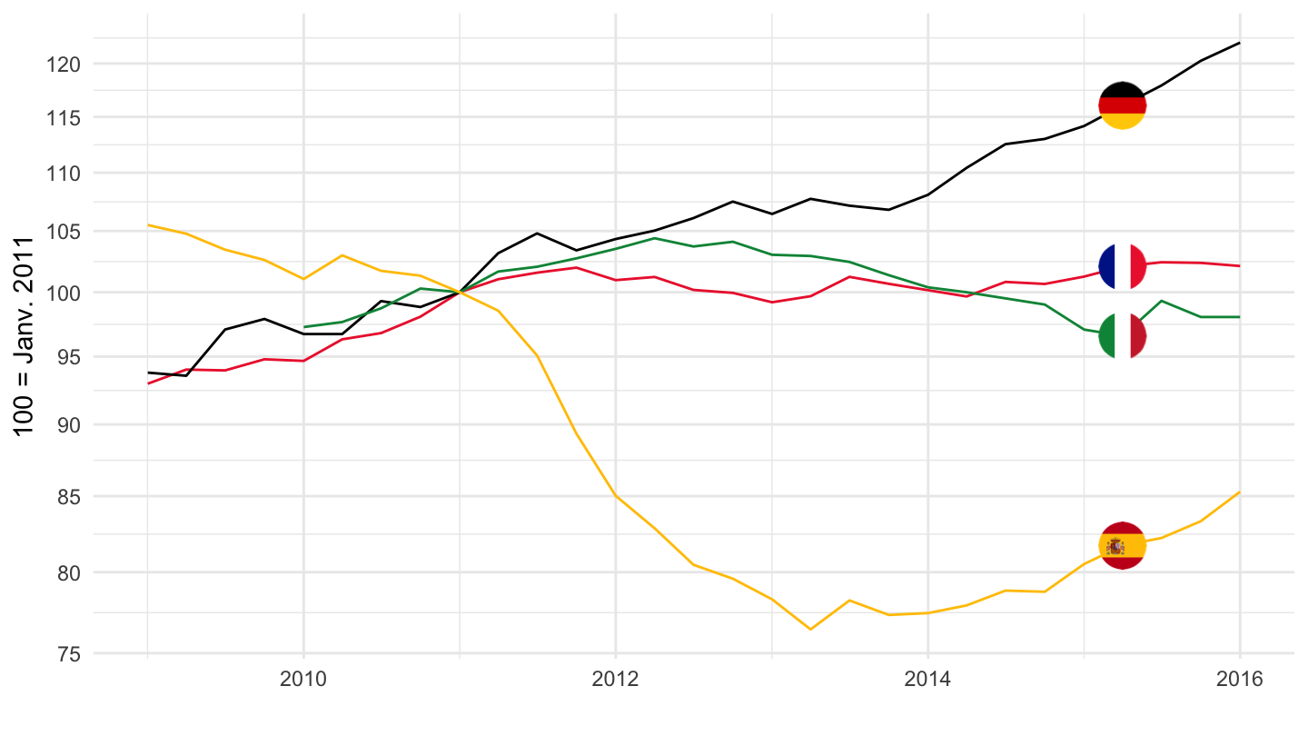
Purchase Total
France, Italy, Germany
Code
prc_hpi_q %>%
  filter(purchase == "TOTAL",
         geo %in% c("FR", "IT", "DE"),
         unit == "I15_Q") %>%
  quarter_to_date %>%

  left_join(colors, by = c("Geo" = "country")) %>%
  ggplot() + geom_line(aes(x = date, y = values, color = color)) +
  theme_minimal() +
  scale_color_identity() +
  scale_x_date(breaks = seq(1920, 2100, 2) %>% paste0("-01-01") %>% as.Date,
               labels = date_format("%Y")) +
  add_4flags +
  theme(legend.position = c(0.35, 0.9),
        legend.title = element_blank()) +
  scale_y_log10(breaks = seq(-100, 300, 10)) +
  ylab("House Price Index") + xlab("")
Belgium, Denmark, Finland
Code
prc_hpi_q %>%
  filter(purchase == "TOTAL",
         geo %in% c("BE", "DK", "FI"),
         unit == "I15_Q") %>%
  quarter_to_date %>%

  ggplot() + geom_line() + theme_minimal() +
  aes(x = date, y = values, color = Geo, linetype = Geo) +
  scale_color_manual(values = viridis(4)[1:3]) +
  scale_x_date(breaks = seq(1920, 2100, 2) %>% paste0("-01-01") %>% as.Date,
               labels = date_format("%Y")) +
  theme(legend.position = c(0.35, 0.9),
        legend.title = element_blank()) +
  scale_y_log10(breaks = seq(-100, 300, 10)) +
  ylab("House Price Index") + xlab("")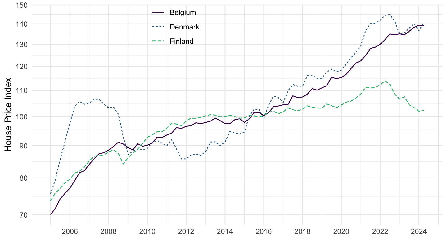
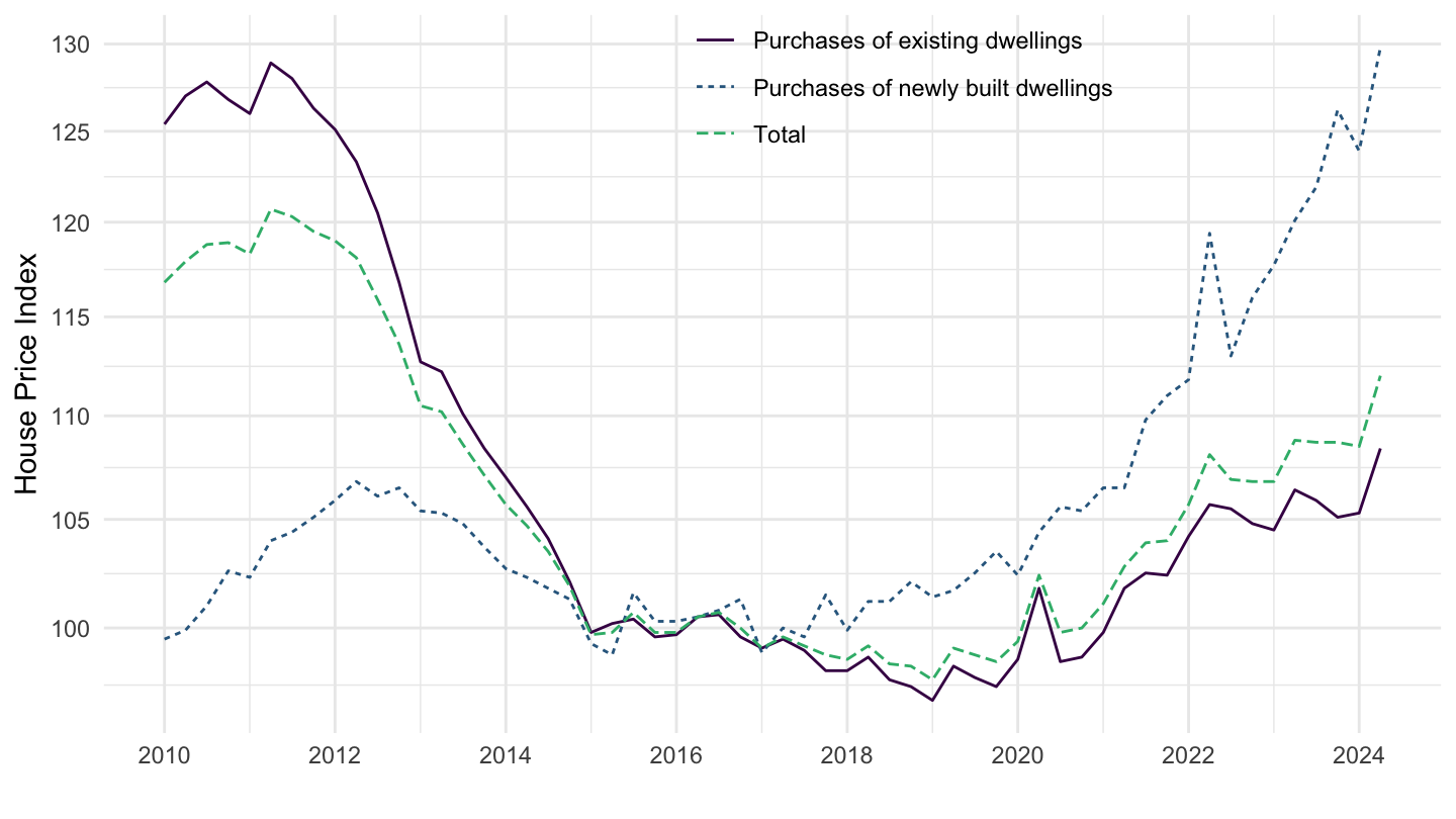
All Series
France
Code
prc_hpi_q %>%
  filter(geo %in% c("FR"),
         unit == "I15_Q") %>%
  quarter_to_date %>%


  ggplot() + geom_line() + theme_minimal() +
  aes(x = date, y = values, color = Purchase, linetype = Purchase) +
  scale_color_manual(values = viridis(4)[1:3]) +
  scale_x_date(breaks = seq(1920, 2100, 2) %>% paste0("-01-01") %>% as.Date,
               labels = date_format("%Y")) +
  theme(legend.position = c(0.35, 0.9),
        legend.title = element_blank()) +
  scale_y_log10(breaks = seq(-100, 300, 10)) +
  ylab("House Price Index") + xlab("")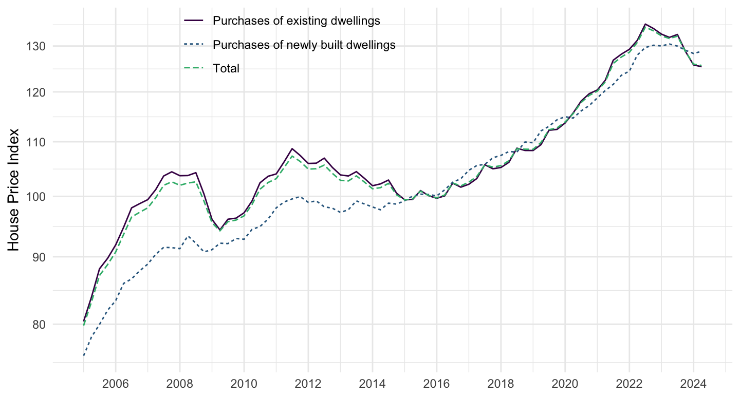
Germany
Code
prc_hpi_q %>%
  filter(geo %in% c("DE"),
         unit == "I15_Q") %>%
  quarter_to_date %>%


  ggplot() + geom_line() + theme_minimal() +
  aes(x = date, y = values, color = Purchase, linetype = Purchase) +
  scale_color_manual(values = viridis(4)[1:3]) +
  scale_x_date(breaks = seq(1920, 2100, 2) %>% paste0("-01-01") %>% as.Date,
               labels = date_format("%Y")) +
  theme(legend.position = c(0.35, 0.9),
        legend.title = element_blank()) +
  scale_y_log10(breaks = seq(-100, 300, 10)) +
  ylab("House Price Index") + xlab("")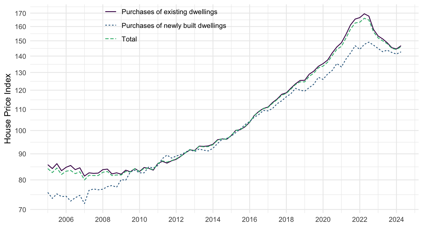
Italy
Code
prc_hpi_q %>%
  filter(geo %in% c("IT"),
         unit == "I15_Q") %>%
  quarter_to_date %>%


  ggplot() + geom_line() + theme_minimal() +
  aes(x = date, y = values, color = Purchase, linetype = Purchase) +
  scale_color_manual(values = viridis(4)[1:3]) +
  scale_x_date(breaks = seq(1920, 2100, 2) %>% paste0("-01-01") %>% as.Date,
               labels = date_format("%Y")) +
  theme(legend.position = c(0.6, 0.9),
        legend.title = element_blank()) +
  scale_y_log10(breaks = seq(-100, 300, 5)) +
  ylab("House Price Index") + xlab("")