| LAST_COMPILE |
|---|
| 2026-07-23 |
House Prices
Data - Fred
Info
LAST_COMPILE
Last
| date | Nobs |
|---|---|
| 2026-06-01 | 8 |
| 2026-05-01 | 9 |
variable
| variable | Variable | Nobs |
|---|---|---|
| CPIAUCSL | Consumer Price Index for All Urban Consumers: All Items in U.S. City Average | 954 |
| CPILFESL | Consumer Price Index for All Urban Consumers: All Items Less Food and Energy in U.S. City Average | 834 |
| CSUSHPINSA | S&P Cotality Case-Shiller U.S. National Home Price Index | 616 |
| MICH | University of Michigan: Inflation Expectation | 581 |
| CUSR0000SEHA | Consumer Price Index for All Urban Consumers: Rent of Primary Residence in U.S. City Average | 546 |
| CUSR0000SAS2RS | Consumer Price Index for All Urban Consumers: Rent of Shelter in U.S. City Average | 438 |
| ASTMA | All Sectors; Total Mortgages; Asset, Level | 322 |
| CP00MI15EA20M086NEST | Harmonized Index of Consumer Prices: Total for Euro Area (20 Countries) | 319 |
| CP041MI15EA20M086NEST | Harmonized Index of Consumer Prices: Actual Rentals for Housing for Euro Area (20 Countries) | 319 |
| TOTNRGFOODEA20MI15XM | Harmonized Index of Consumer Prices: Overall Index Excluding Energy, Food, Alcohol, and Tobacco for Euro Area (20 Countries) | 319 |
| A255RD3Q086SBEA | Imports of goods (implicit price deflator) | 317 |
| DPCCRV1Q225SBEA | Personal Consumption Expenditures (PCE) Excluding Food and Energy (Chain-Type Price Index) | 268 |
| MSPUS | Median Sales Price of Houses Sold for the United States | 253 |
| USSTHPI | All-Transactions House Price Index for the United States | 205 |
| CDSP | Consumer Debt Service Payments as a Percent of Disposable Personal Income | 185 |
| MDSP | Mortgage Debt Service Payments as a Percent of Disposable Personal Income | 185 |
| TDSP | Household Debt Service Payments as a Percent of Disposable Personal Income | 185 |
| FPCPITOTLZGUSA | Inflation, consumer prices for the United States | 65 |
| FIXHAI | Housing Affordability Index (Fixed) | 14 |
Housing Affordability Index
Code
housing %>%
  filter(variable %in% c("FIXHAI")) %>%
  ggplot(.) + geom_line(aes(x = date, y = value)) +
  theme_minimal() + xlab("") + ylab("Housing Affordability Index") +
  scale_x_date(breaks = "1 month",
               labels = date_format("%Y %b")) +
  scale_y_log10(breaks = seq(10, 400, 2)) +
  theme(legend.position = c(0.3, 0.9),
        legend.title = element_blank(),
        axis.text.x = element_text(angle = 45, vjust = 1, hjust = 1)) +
  geom_hline(yintercept = 100, linetype = "dashed",  color = "black")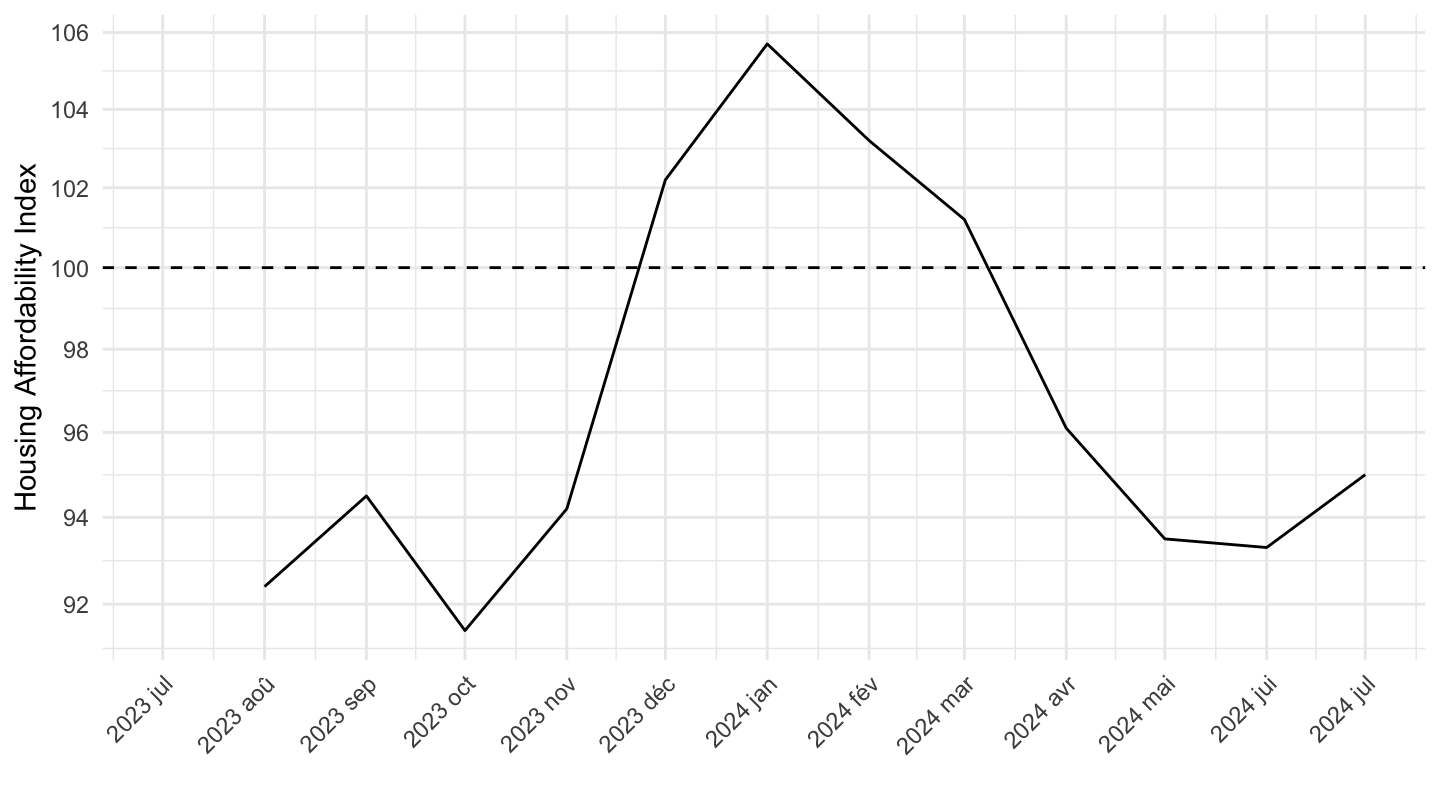
Rents
inflation
12 months
English
Code
housing %>%
  filter(variable %in% c("CP041MI15EA20M086NEST", "CUSR0000SEHA",
                         "CP00MI15EA20M086NEST", "CPIAUCSL")) %>%
  #add_row(date = as.Date("2023-10-01"), variable = "CP00MI15EA20M086NEST", value = 124.55) %>%
  select(date, variable, value) %>%
  group_by(variable) %>%
  arrange(date) %>%
  mutate(value = value/lag(value, 12)-1) %>%
  filter(date >= as.Date("2012-01-01")) %>%
  ungroup %>%
  mutate(type = case_when(variable  %in% c("CP041MI15EA20M086NEST", "CUSR0000SEHA") ~ "Rents",
                          variable  %in% c("CP00MI15EA20M086NEST", "CPIAUCSL") ~ "All")) %>%
  mutate(country = case_when(variable %in% c("CP041MI15EA20M086NEST", "CP00MI15EA20M086NEST") ~ "Euro area (HICP)",
                              variable %in% c("CUSR0000SEHA", "CPIAUCSL") ~ "US (CPI)")) %>%
  ggplot(.) + geom_line(aes(x = date, y = value, linetype = type, color = country)) +
  theme_minimal() + xlab("") + ylab("Inflation (%)") +
  scale_x_date(breaks = seq(1870, 2100, 1) %>% paste0("-01-01") %>% as.Date,
               labels = scales::date_format("%Y")) +
  scale_y_continuous(breaks = 0.01*seq(-60, 60, 1),
                     labels = scales::percent_format(accuracy = 1)) +
  scale_color_manual(values = c("#003399", "#B22234")) +
  theme(legend.position = c(0.2, 0.8),
        legend.title = element_blank())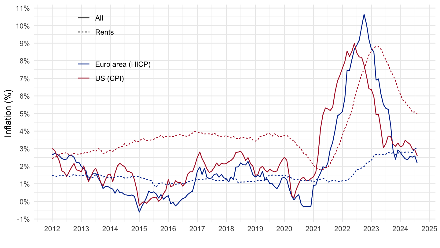
French
All
Code
Sys.setlocale("LC_TIME", "fr_CA.UTF-8")# [1] "fr_CA.UTF-8"Code
housing %>%
  filter(variable %in% c("CP041MI15EA20M086NEST", "CUSR0000SEHA",
                         "CP00MI15EA20M086NEST", "CPIAUCSL")) %>%
  #add_row(date = as.Date("2023-10-01"), variable = "CP00MI15EA20M086NEST", value = 124.55) %>%
  select(date, variable, value) %>%
  group_by(variable) %>%
  arrange(date) %>%
  mutate(value = value/lag(value, 12)-1) %>%
  filter(date >= as.Date("2012-01-01")) %>%
  ungroup %>%
  mutate(type = case_when(variable  %in% c("CP041MI15EA20M086NEST", "CUSR0000SEHA") ~ "Loyers",
                          variable  %in% c("CP00MI15EA20M086NEST", "CPIAUCSL") ~ "Tous")) %>%
  mutate(country = case_when(variable %in% c("CP041MI15EA20M086NEST", "CP00MI15EA20M086NEST") ~ "Zone euro (IPCH)",
                              variable %in% c("CUSR0000SEHA", "CPIAUCSL") ~ "États-Unis (CPI)")) %>%
  mutate(country = factor(country, levels = c("Zone euro (IPCH)", "États-Unis (CPI)")),
         type = factor(type, levels = c("Tous", "Loyers"))) %>%
  ggplot(.) + geom_line(aes(x = date, y = value, linetype = type, color = country)) +
  theme_minimal() + xlab("") + ylab("Inflation (%)") +
  scale_x_date(breaks = seq(1870, 2100, 1) %>% paste0("-01-01") %>% as.Date,
               labels = scales::date_format("%Y")) +
  scale_y_continuous(breaks = 0.01*seq(-60, 60, 1),
                     labels = scales::percent_format(accuracy = 1)) +
  scale_color_manual(values = c("#003399", "#B22234")) +
  scale_linetype_manual(values = c("dashed", "solid")) +
  theme(legend.position = c(0.2, 0.8),
        legend.title = element_blank())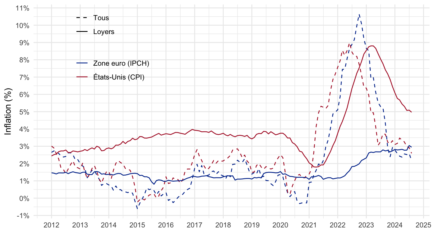
Code
Sys.setlocale("LC_TIME", "en_CA.UTF-8")# [1] "en_CA.UTF-8"6 months
Code
housing %>%
  filter(variable %in% c("CP041MI15EA20M086NEST", "CUSR0000SEHA",
                         "CP00MI15EA20M086NEST", "CPIAUCSL",
                         "TOTNRGFOODEA20MI15XM", "CPILFESL")) %>%
  #add_row(date = as.Date("2023-10-01"), variable = "CP00MI15EA20M086NEST", value = 124.55) %>%
  select(date, variable, value) %>%
  group_by(variable) %>%
  arrange(date) %>%
  mutate(value = value/lag(value, 6)-1) %>%
  filter(date >= as.Date("2012-01-01")) %>%
  ungroup %>%
  mutate(type = case_when(variable  %in% c("CP041MI15EA20M086NEST", "CUSR0000SEHA") ~ "Rents",
                          variable  %in% c("CP00MI15EA20M086NEST", "CPIAUCSL") ~ "All",
                          variable  %in% c("TOTNRGFOODEA20MI15XM", "CPILFESL") ~ "Core")) %>%
  mutate(country = case_when(variable %in% c("CP041MI15EA20M086NEST", "CP00MI15EA20M086NEST", "TOTNRGFOODEA20MI15XM") ~ "Euro area (HICP)",
                              variable %in% c("CUSR0000SEHA", "CPIAUCSL", "CPILFESL") ~ "US (CPI)")) %>%
  ggplot(.) + geom_line(aes(x = date, y = value, linetype = type, color = country)) +
  theme_minimal() + xlab("") + ylab("Inflation, 6 months (%)") +
  scale_x_date(breaks = seq(1870, 2100, 1) %>% paste0("-01-01") %>% as.Date,
               labels = scales::date_format("%Y")) +
  scale_y_continuous(breaks = 0.01*seq(-60, 60, 1),
                     labels = scales::percent_format(accuracy = 1)) +
  scale_color_manual(values = c("#003399", "#B22234")) +
  theme(legend.position = c(0.2, 0.8),
        legend.title = element_blank())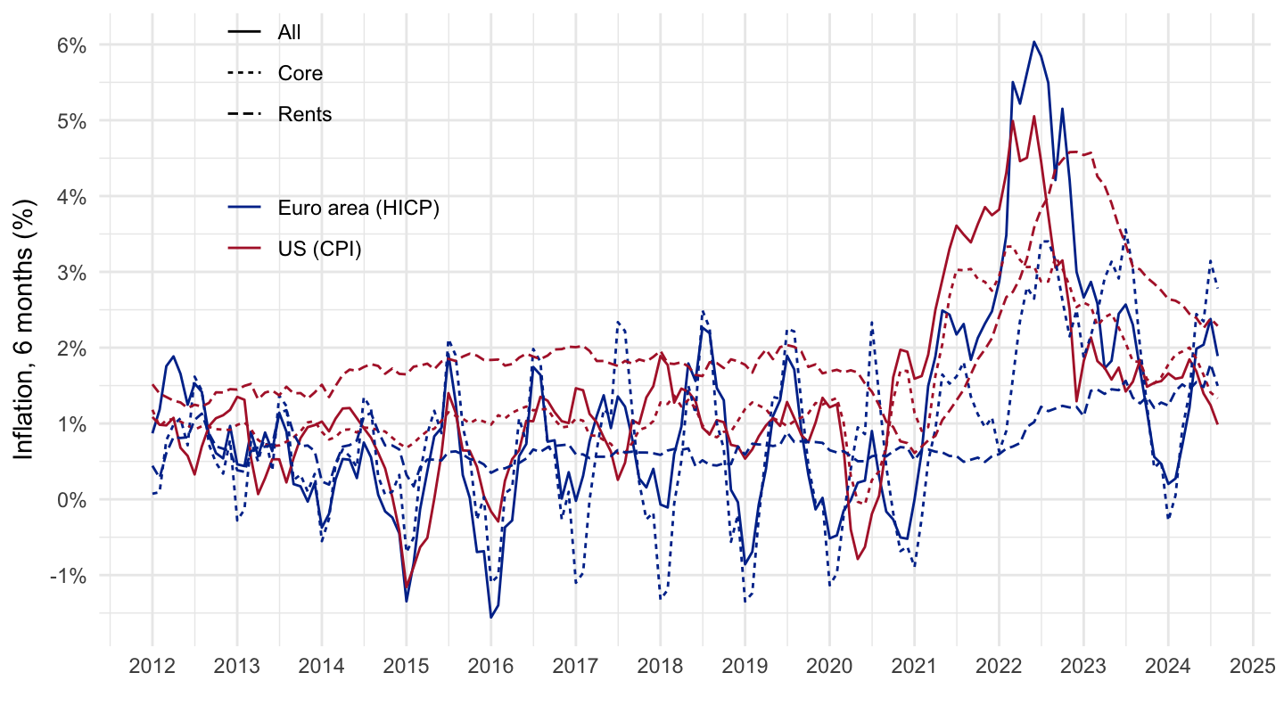
3 months
Code
housing %>%
  filter(variable %in% c("CP041MI15EA20M086NEST", "CUSR0000SEHA",
                         "CP00MI15EA20M086NEST", "CPIAUCSL",
                         "TOTNRGFOODEA20MI15XM", "CPILFESL")) %>%
  #add_row(date = as.Date("2023-10-01"), variable = "CP00MI15EA20M086NEST", value = 124.55) %>%
  select(date, variable, value) %>%
  group_by(variable) %>%
  arrange(date) %>%
  mutate(value = value/lag(value, 3)-1) %>%
  filter(date >= as.Date("2012-01-01")) %>%
  ungroup %>%
  mutate(type = case_when(variable  %in% c("CP041MI15EA20M086NEST", "CUSR0000SEHA") ~ "Rents",
                          variable  %in% c("CP00MI15EA20M086NEST", "CPIAUCSL") ~ "All",
                          variable  %in% c("TOTNRGFOODEA20MI15XM", "CPILFESL") ~ "Core")) %>%
  mutate(country = case_when(variable %in% c("CP041MI15EA20M086NEST", "CP00MI15EA20M086NEST", "TOTNRGFOODEA20MI15XM") ~ "Euro area (HICP)",
                              variable %in% c("CUSR0000SEHA", "CPIAUCSL", "CPILFESL") ~ "US (CPI)")) %>%
  ggplot(.) + geom_line(aes(x = date, y = value, linetype = type, color = country)) +
  theme_minimal() + xlab("") + ylab("Inflation, 3 months (%)") +
  scale_x_date(breaks = seq(1870, 2100, 1) %>% paste0("-01-01") %>% as.Date,
               labels = scales::date_format("%Y")) +
  scale_y_continuous(breaks = 0.01*seq(-60, 60, 1),
                     labels = scales::percent_format(accuracy = 1)) +
  scale_color_manual(values = c("#003399", "#B22234")) +
  theme(legend.position = c(0.2, 0.8),
        legend.title = element_blank())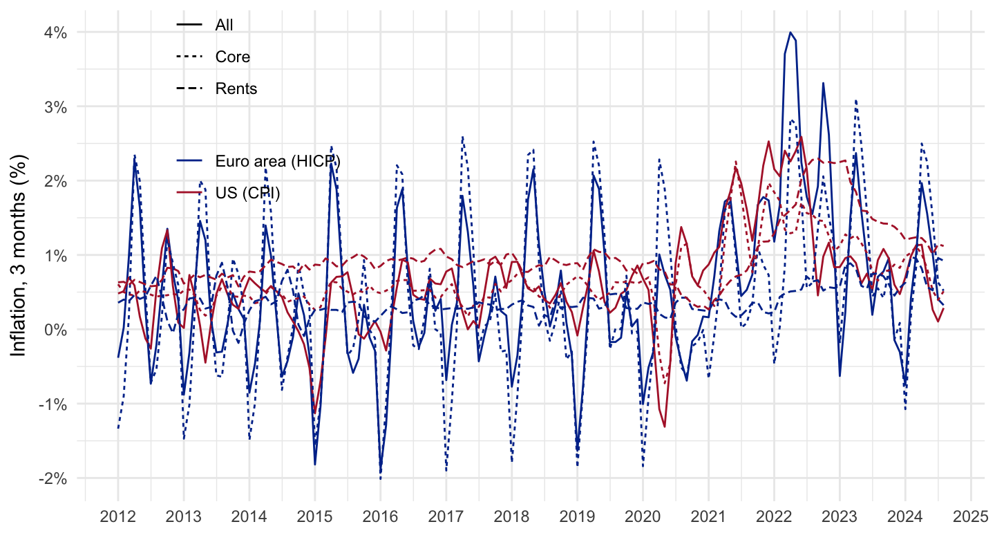
Price index
Just housing
Code
housing %>%
  filter(variable %in% c("CP041MI15EA20M086NEST", "CUSR0000SEHA"),
         date >= as.Date("2020-01-01")) %>%
  select(date, variable, value) %>%
  group_by(variable) %>%
  arrange(date) %>%
  mutate(value = 100*value/value[1]) %>%
  ungroup %>%
  mutate(Variable = case_when(variable == "CP041MI15EA20M086NEST" ~ "Euro area HICP Rents",
                              variable == "CUSR0000SEHA" ~ "US CPI Rents")) %>%
  ggplot(.) + geom_line(aes(x = date, y = value, color = Variable)) +
  theme_minimal() + xlab("") + ylab("Price Index") +
  scale_x_date(breaks = seq(1870, 2100, 1) %>% paste0("-01-01") %>% as.Date,
               labels = scales::date_format("%Y")) +
  scale_y_log10(breaks = seq(100, 200, 2)) +
  scale_color_manual(values = c("#2D68C4", "#F2A900", "#000000")) +
  theme(legend.position = c(0.2, 0.8),
        legend.title = element_blank())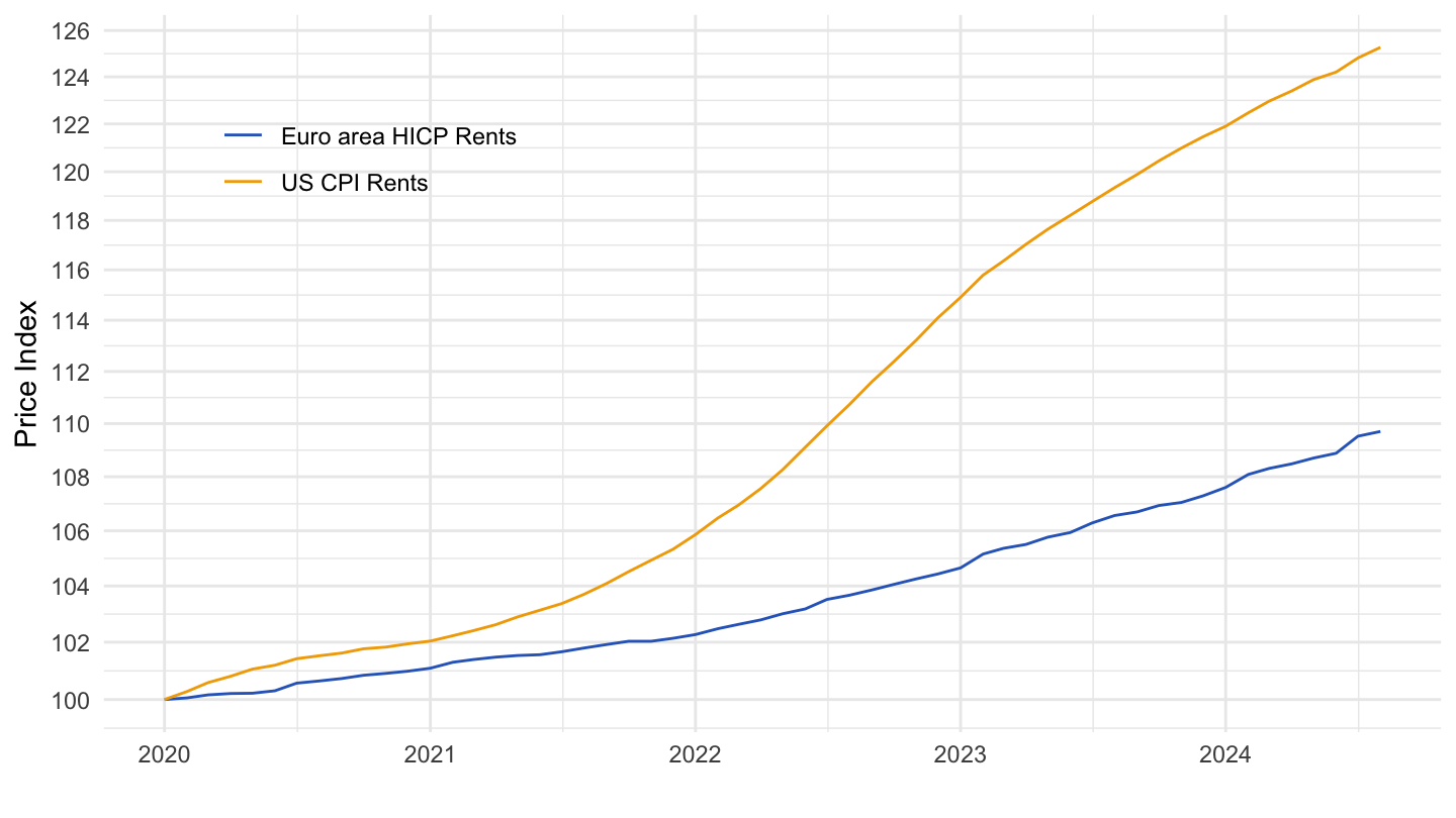
Real House Prices
Growth
Code
housing %>%
  filter(variable %in% c("CPIAUCSL", "CSUSHPINSA"),
         month(date) == 1,
         date >= as.Date("1987-01-01")) %>%
  select(date, variable, value) %>%
  spread(variable, value) %>%
  mutate(CPIAUCSL = 100*(log(CPIAUCSL) - lag(log(CPIAUCSL))),
         CSUSHPINSA = 100*(log(CSUSHPINSA) - lag(log(CSUSHPINSA)))) %>%
  gather(variable, value, -date) %>%
  left_join(variable, by = "variable") %>%
  ggplot(.) + geom_line(aes(x = date, y = value / 100, color = Variable)) +
  theme_minimal() + xlab("") + ylab("Inflation Rates (%)") +
  scale_x_date(breaks = seq(1870, 2100, 5) %>% paste0("-01-01") %>% as.Date,
               labels = date_format("%Y")) +
  scale_y_continuous(breaks = 0.01*seq(-60, 60, 2),
                     labels = scales::percent_format(accuracy = 1)) +
  scale_color_manual(values = c("#2D68C4", "#F2A900", "#000000")) +
  theme(legend.position = c(0.4, 0.2),
        legend.title = element_blank())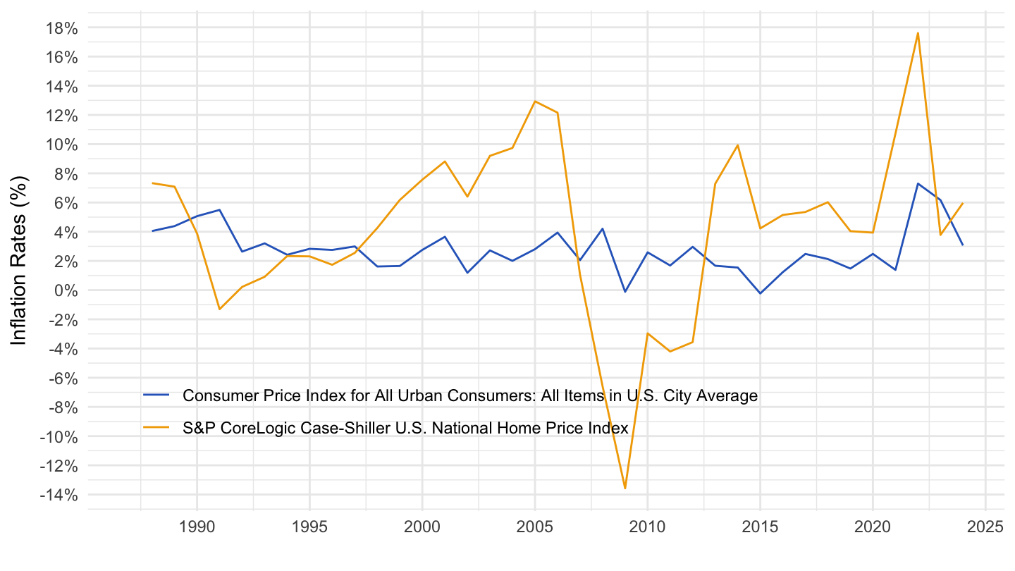
Index
Code
housing %>%
  filter(variable %in% c("CPIAUCSL", "CSUSHPINSA"),
         date >= as.Date("2000-01-01")) %>%
  select(date, variable, value) %>%
  spread(variable, value) %>%
  mutate(`Nominal S&P/Case-Shiller Index` = CSUSHPINSA,
         CSUSHPINSA_real = CSUSHPINSA/CPIAUCSL,
         `Real S&P/Case-Shiller Index` = 100*CSUSHPINSA_real / CSUSHPINSA_real[1]) %>%
  select(date, `Nominal S&P/Case-Shiller Index`, `Real S&P/Case-Shiller Index`) %>%
  gather(variable, value, -date) %>%
  group_by(variable) %>%
  mutate(value = 100*value/value[date == as.Date("2006-10-01")]) %>%
  ggplot(.) + geom_line(aes(x = date, y = value, color = variable)) +
  theme_minimal() + xlab("") + ylab("S&P/Case-Shiller Index (Nov. 2006 Peak = 100)") +
  scale_x_date(breaks = seq(1870, 2100, 2) %>% paste0("-01-01") %>% as.Date,
               labels = date_format("%Y")) +
  scale_y_log10(breaks = seq(10, 400, 10)) +
  scale_color_manual(values = c("#2D68C4", "#F2A900", "#000000")) +
  theme(legend.position = c(0.2, 0.9),
        legend.title = element_blank()) +
  geom_hline(yintercept = 100, linetype = "dashed",  color = "black")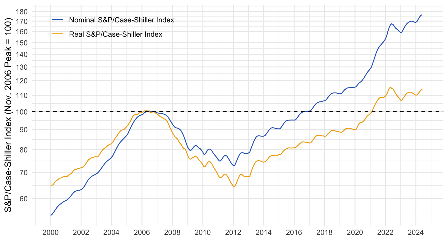
Median House Prices
All
Code
housing %>%
  filter(variable %in% c("MSPUS", "CPIAUCSL"),
         date >= as.Date("1965-01-01"),
         month(date) %in% c(1, 4, 7, 10)) %>%
  select(date, variable, value) %>%
  spread(variable, value) %>%
  mutate(`Nominal Median Sales Price of Houses` = MSPUS,
         MSPUS_real = MSPUS/CPIAUCSL,
         `Real Median Sales Price of Houses` = 100*MSPUS_real / MSPUS_real[1]) %>%
  select(date, `Nominal Median Sales Price of Houses`, `Real Median Sales Price of Houses`) %>%
  gather(variable, value, -date) %>%
  group_by(variable) %>%
  mutate(value = 100*value/value[date == as.Date("2007-01-01")]) %>%
  ggplot(.) + geom_line(aes(x = date, y = value, color = variable)) +
  theme_minimal() + xlab("") + ylab("Median Sales Price of Houses (2007 = 100)") +
  scale_x_date(breaks = seq(1870, 2100, 5) %>% paste0("-01-01") %>% as.Date,
               labels = date_format("%Y")) +
  scale_y_log10(breaks = seq(10, 400, 10)) +
  scale_color_manual(values = c("#2D68C4", "#F2A900", "#000000")) +
  theme(legend.position = c(0.3, 0.9),
        legend.title = element_blank()) +
  geom_hline(yintercept = 100, linetype = "dashed",  color = "black")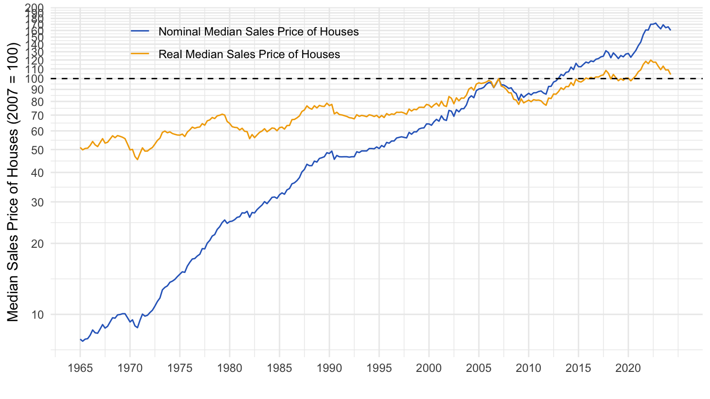
1980-
Code
housing %>%
  filter(variable %in% c("MSPUS", "CPIAUCSL"),
         date >= as.Date("1980-01-01"),
         month(date) %in% c(1, 4, 7, 10)) %>%
  select(date, variable, value) %>%
  spread(variable, value) %>%
  mutate(`Nominal Median Sales Price of Houses` = MSPUS,
         MSPUS_real = MSPUS/CPIAUCSL,
         `Real Median Sales Price of Houses` = 100*MSPUS_real / MSPUS_real[1]) %>%
  select(date, `Nominal Median Sales Price of Houses`, `Real Median Sales Price of Houses`) %>%
  gather(variable, value, -date) %>%
  group_by(variable) %>%
  mutate(value = 100*value/value[date == as.Date("2007-01-01")]) %>%
  ggplot(.) + geom_line(aes(x = date, y = value, color = variable)) +
  theme_minimal() + xlab("") + ylab("Median Sales Price of Houses (2007 = 100)") +
  scale_x_date(breaks = seq(1870, 2100, 5) %>% paste0("-01-01") %>% as.Date,
               labels = date_format("%Y")) +
  scale_y_log10(breaks = seq(10, 400, 10)) +
  scale_color_manual(values = c("#2D68C4", "#F2A900", "#000000")) +
  theme(legend.position = c(0.3, 0.9),
        legend.title = element_blank()) +
  geom_hline(yintercept = 100, linetype = "dashed",  color = "black")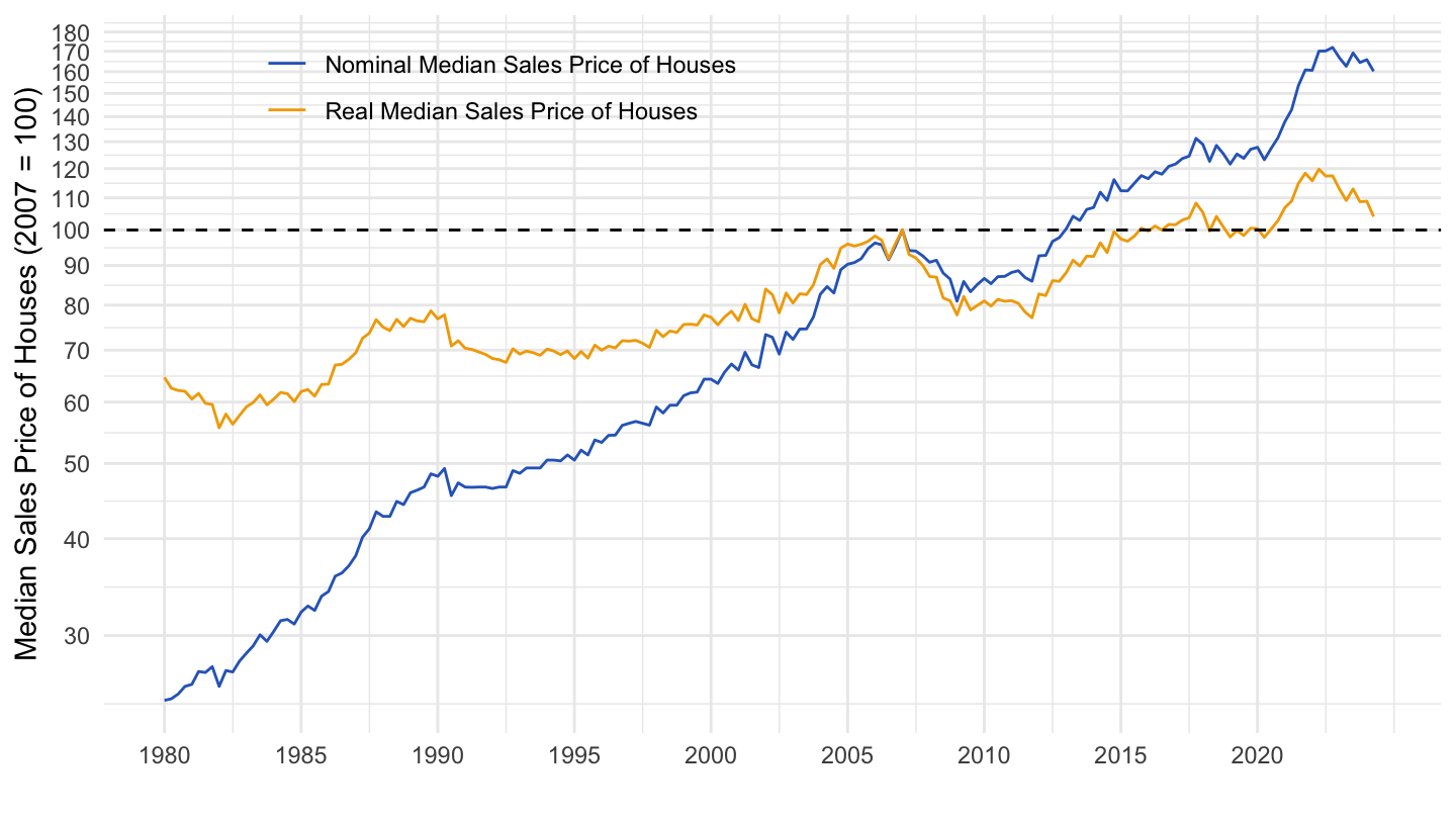
1990-
Code
housing %>%
  filter(variable %in% c("MSPUS", "CPIAUCSL"),
         date >= as.Date("1990-01-01"),
         month(date) %in% c(1, 4, 7, 10)) %>%
  select(date, variable, value) %>%
  spread(variable, value) %>%
  mutate(`Nominal Median Sales Price of Houses` = MSPUS,
         MSPUS_real = MSPUS/CPIAUCSL,
         `Real Median Sales Price of Houses` = 100*MSPUS_real / MSPUS_real[1]) %>%
  select(date, `Nominal Median Sales Price of Houses`, `Real Median Sales Price of Houses`) %>%
  gather(variable, value, -date) %>%
  group_by(variable) %>%
  mutate(value = 100*value/value[date == as.Date("2007-01-01")]) %>%
  ggplot(.) + geom_line(aes(x = date, y = value, color = variable)) +
  theme_minimal() + xlab("") + ylab("Median Sales Price of Houses (2007 = 100)") +
  scale_x_date(breaks = seq(1870, 2100, 5) %>% paste0("-01-01") %>% as.Date,
               labels = date_format("%Y")) +
  scale_y_log10(breaks = seq(10, 400, 10)) +
  scale_color_manual(values = c("#2D68C4", "#F2A900", "#000000")) +
  theme(legend.position = c(0.3, 0.9),
        legend.title = element_blank()) +
  geom_hline(yintercept = 100, linetype = "dashed",  color = "black")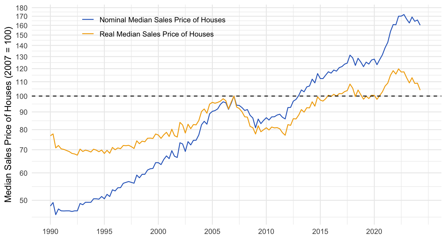
2000-
Code
housing %>%
  filter(variable %in% c("MSPUS", "CPIAUCSL"),
         date >= as.Date("2000-01-01"),
         month(date) %in% c(1, 4, 7, 10)) %>%
  select(date, variable, value) %>%
  spread(variable, value) %>%
  mutate(`Nominal Median Sales Price of Houses` = MSPUS,
         MSPUS_real = MSPUS/CPIAUCSL,
         `Real Median Sales Price of Houses` = 100*MSPUS_real / MSPUS_real[1]) %>%
  select(date, `Nominal Median Sales Price of Houses`, `Real Median Sales Price of Houses`) %>%
  gather(variable, value, -date) %>%
  group_by(variable) %>%
  mutate(value = 100*value/value[date == as.Date("2007-01-01")]) %>%
  ggplot(.) + geom_line(aes(x = date, y = value, color = variable)) +
  theme_minimal() + xlab("") + ylab("Median Sales Price of Houses (2007 = 100)") +
  scale_x_date(breaks = seq(1870, 2100, 2) %>% paste0("-01-01") %>% as.Date,
               labels = date_format("%Y")) +
  scale_y_log10(breaks = seq(10, 400, 10)) +
  scale_color_manual(values = c("#2D68C4", "#F2A900", "#000000")) +
  theme(legend.position = c(0.3, 0.9),
        legend.title = element_blank()) +
  geom_hline(yintercept = 100, linetype = "dashed",  color = "black")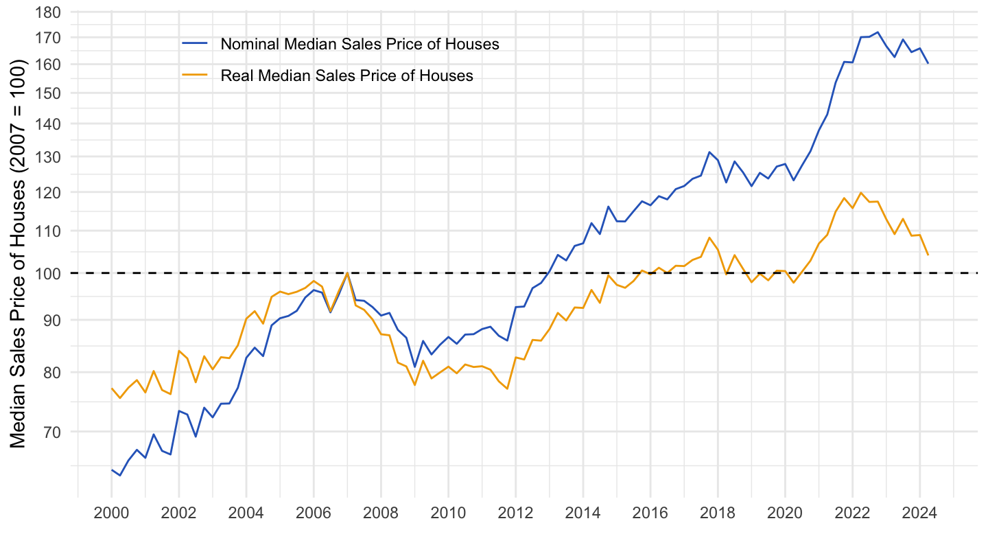
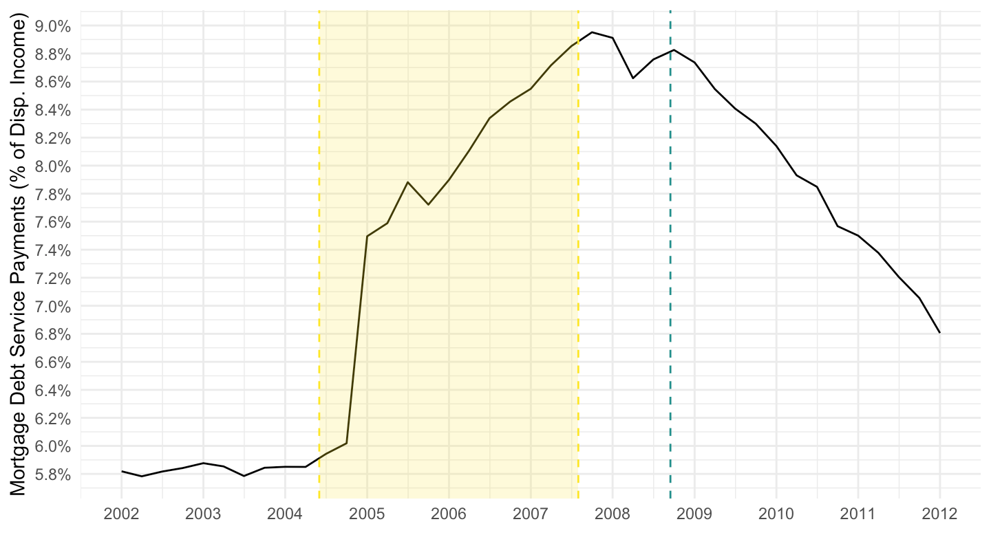
Mortgage Debt Service Payments (% Disposable Personal Income)
All
Code
housing %>%
  filter(variable %in% c("MDSP")) %>%
  mutate(value = value / 100) %>%
  ggplot(.) + geom_line(aes(x = date, y = value)) + theme_minimal() +
  scale_x_date(breaks = seq(1870, 2022, 5) %>% paste0("-01-01") %>% as.Date,
               labels = date_format("%Y")) +
  scale_y_continuous(breaks = 0.01*seq(0, 15, 0.2),
                     labels = scales::percent_format(accuracy = 0.1)) +
  xlab("") + ylab("% of Disposable Income") +
  geom_vline(xintercept = as.Date("2008-09-15"), linetype = "dashed", color = viridis(3)[2]) +
    geom_rect(data = data_frame(start = as.Date("2004-06-01"),
                                end = as.Date("2007-08-01")),
              aes(xmin = start, xmax = end, ymin = -Inf, ymax = +Inf),
              fill = viridis(4)[4], alpha = 0.2) +
    geom_vline(xintercept = as.Date("2004-06-01"), linetype = "dashed", color = viridis(4)[4]) +
    geom_vline(xintercept = as.Date("2007-08-01"), linetype = "dashed", color = viridis(4)[4])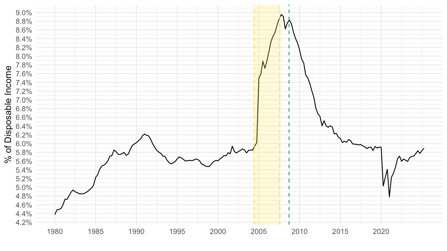
2000-
Code
housing %>%
  filter(variable %in% c("MDSP"),
         date >= as.Date("1994-01-01")) %>%
  mutate(value = value / 100) %>%
  ggplot(.) + geom_line(aes(x = date, y = value)) + theme_minimal() +
  scale_x_date(breaks = seq(1870, 2100, 2) %>% paste0("-01-01") %>% as.Date,
               labels = date_format("%Y")) +
  scale_y_continuous(breaks = 0.01*seq(0, 15, 0.2),
                     labels = scales::percent_format(accuracy = 0.1)) +
  xlab("") + ylab("Mortgage debt service payments (% of Disposable Income)") +
  geom_vline(xintercept = as.Date("2008-09-15"), linetype = "dashed", color = viridis(3)[2]) +
    geom_rect(data = data_frame(start = as.Date("2004-06-01"),
                                end = as.Date("2007-08-01")),
              aes(xmin = start, xmax = end, ymin = -Inf, ymax = +Inf),
              fill = viridis(4)[4], alpha = 0.2) +
    geom_vline(xintercept = as.Date("2004-06-01"), linetype = "dashed", color = viridis(4)[4]) +
    geom_vline(xintercept = as.Date("2007-08-01"), linetype = "dashed", color = viridis(4)[4])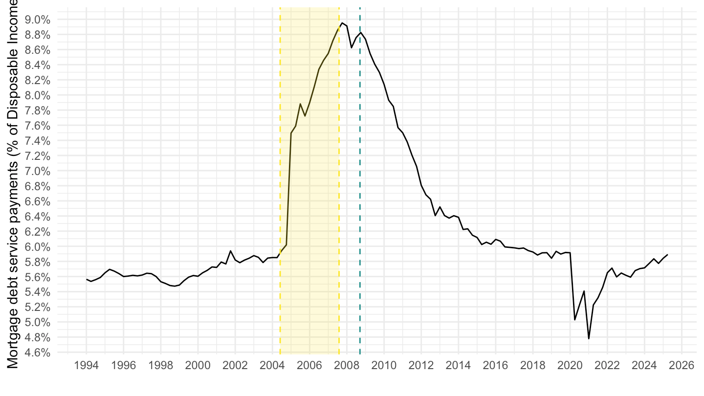
2000-2012
New
Code
housing %>%
  filter(variable %in% c("MDSP")) %>%
  filter(date >= as.Date("2000-01-01"),
         date <= as.Date("2012-01-01")) %>%
  mutate(value = value / 100) %>%
  ggplot(.) + geom_line(aes(x = date, y = value)) + theme_minimal() +
  scale_x_date(breaks = seq(1870, 2100, 1) %>% paste0("-01-01") %>% as.Date,
               labels = date_format("%Y")) +
  scale_y_continuous(breaks = 0.01*seq(0, 15, 0.2),
                     labels = scales::percent_format(accuracy = 0.1)) +
  xlab("") + ylab("% of Disposable Income") +
  geom_vline(xintercept = as.Date("2008-09-15"), linetype = "dashed", color = viridis(3)[2]) +
    geom_rect(data = data_frame(start = as.Date("2004-06-01"),
                                end = as.Date("2007-08-01")),
              aes(xmin = start, xmax = end, ymin = -Inf, ymax = +Inf),
              fill = viridis(4)[4], alpha = 0.2) +
    geom_vline(xintercept = as.Date("2004-06-01"), linetype = "dashed", color = viridis(4)[4]) +
    geom_vline(xintercept = as.Date("2007-08-01"), linetype = "dashed", color = viridis(4)[4])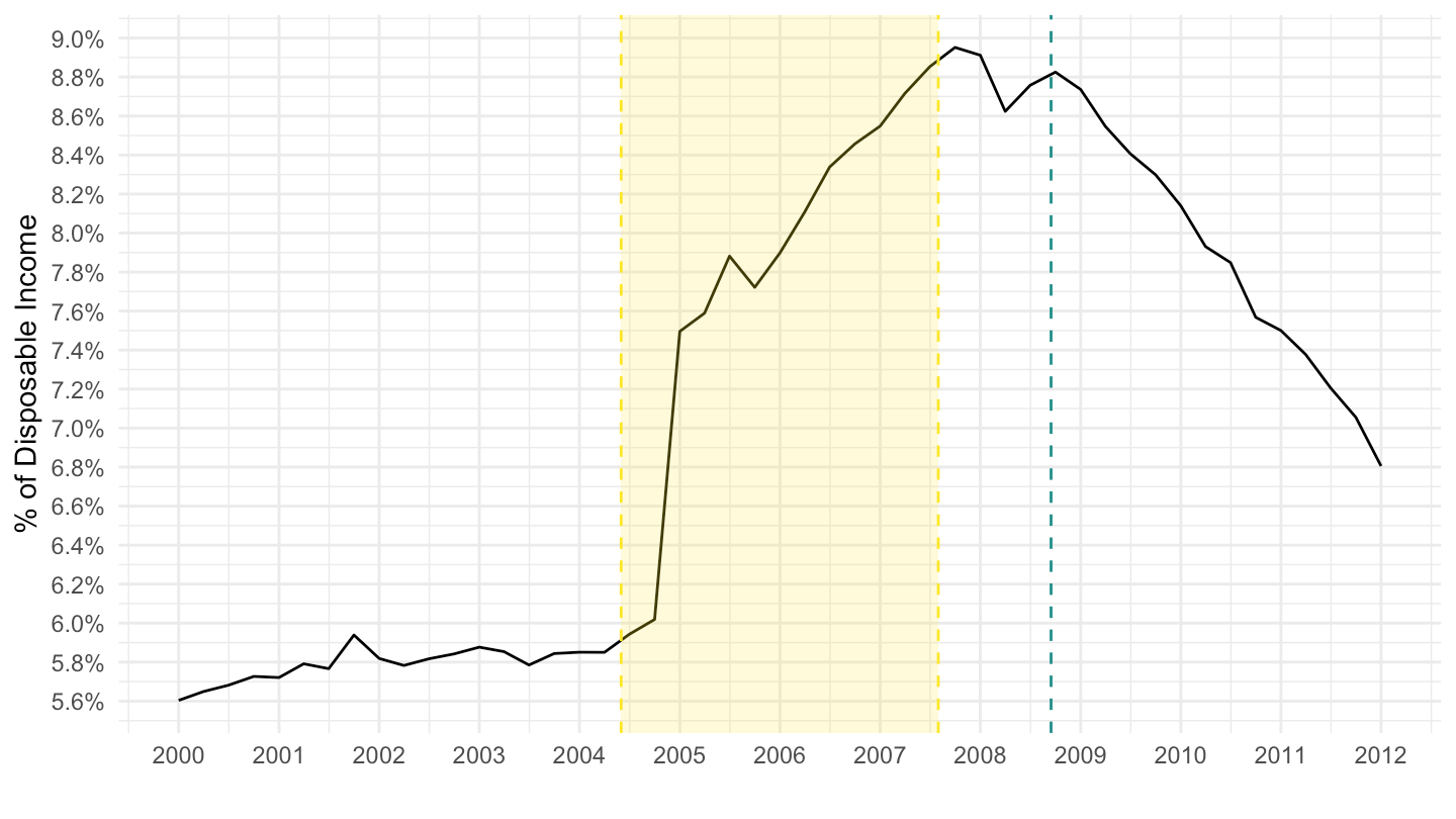
old
Code
housing %>%
  filter(variable %in% c("MDSP")) %>%
  filter(date >= as.Date("2002-01-01"),
         date <= as.Date("2012-01-01")) %>%
  mutate(value = value / 100) %>%
  ggplot(.) + geom_line(aes(x = date, y = value)) + theme_minimal() +
  scale_x_date(breaks = seq(1870, 2100, 1) %>% paste0("-01-01") %>% as.Date,
               labels = date_format("%Y")) +
  scale_y_continuous(breaks = 0.01*seq(0, 15, 0.2),
                     labels = scales::percent_format(accuracy = 0.1)) +
  xlab("") + ylab("Mortgage Debt Service Payments (% of Disp. Income)") +
  geom_vline(xintercept = as.Date("2008-09-15"), linetype = "dashed", color = viridis(3)[2]) +
    geom_rect(data = data_frame(start = as.Date("2004-06-01"),
                                end = as.Date("2007-08-01")),
              aes(xmin = start, xmax = end, ymin = -Inf, ymax = +Inf),
              fill = viridis(4)[4], alpha = 0.2) +
    geom_vline(xintercept = as.Date("2004-06-01"), linetype = "dashed", color = viridis(4)[4]) +
    geom_vline(xintercept = as.Date("2007-08-01"), linetype = "dashed", color = viridis(4)[4])