Taux d’intérêt - France
Données - BDF
Info
Structure
Taux de rémunération
Nobs
Code
MIR1 %>%

  filter(grepl("Taux moyen de rémunération annuel", Variable)) %>%
  group_by(variable, Variable) %>%
  summarise(Nobs = n()) %>%
print_table_conditional()| variable | Variable | Nobs |
|---|---|---|
| MIR1.M.FR.B.L20.A.C.A.2300U6.EUR.O | Taux moyen de rémunération annuel des dépôts bancaires | 266 |
| MIR1.M.FR.B.L20.A.R.A.2300U6.EUR.O | Taux moyen de rémunération annuel des dépôts bancaires | 266 |
| MIR1.M.FR.B.L20.L.C.A.2300U6.EUR.O | Taux moyen de rémunération annuel des dépôts, moins de 2 ans | 266 |
| MIR1.M.FR.B.L20.L.R.A.2300U6.EUR.O | Taux moyen de rémunération annuel des dépôts, moins de 2 ans | 266 |
Taux de rémunération des dépôts + immobilier
Code
MIR1 %>%
  filter(grepl("MIR1.M.FR.B.L20.A.C.A.2300U6.EUR.O", variable) |
           grepl("MIR1.M.FR.B.L20.L.C.A.2300U6.EUR.O", variable)) %>%
  na.omit %>%

  ggplot + geom_line(aes(x = date, y = value/100, color = Variable)) +
  theme_minimal() +
  scale_x_date(breaks = as.Date(paste0(seq(1960, 2100, 1), "-01-01")),
               labels = date_format("%Y")) +
  theme(legend.position = c(0.55, 0.9),
        legend.title = element_blank(),
        legend.direction = "vertical") +
  xlab("") + ylab("Taux d'intérêt (%)") +
  scale_y_continuous(breaks = 0.01*seq(-10, 100, .1),
                labels = percent_format(accuracy = .1))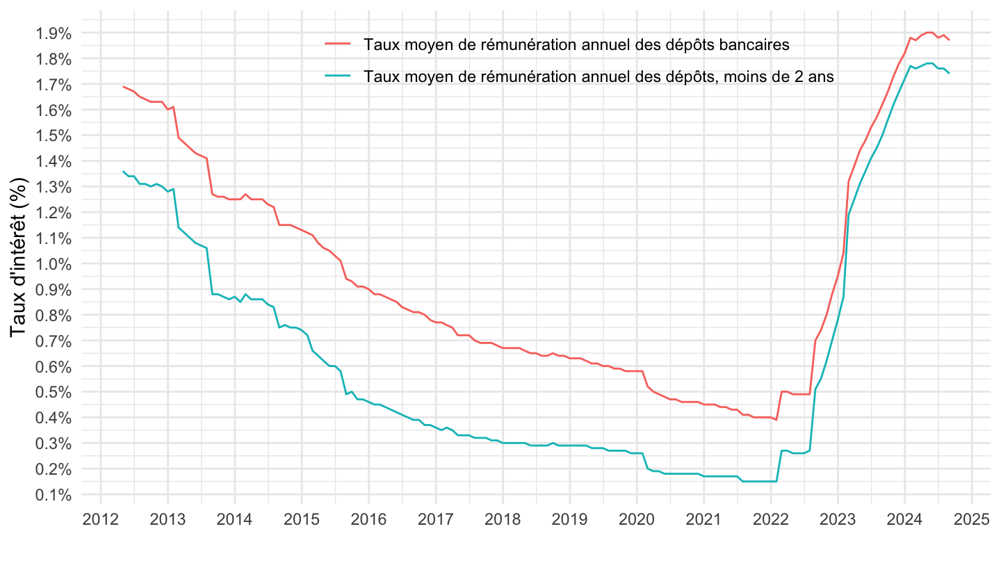
Taux
Nobs
Code
MIR1 %>%

  filter(FREQ == "M",
         REF_AREA == "FR",
         BS_ITEM == "A22") %>%
  group_by(variable, Variable) %>%
  summarise(Nobs = n()) %>%
print_table_conditional()| variable | Variable | Nobs |
|---|---|---|
| MIR1.M.FR.B.A22.A.5.A.2250U6.EUR.N | Crédits nouveaux à l'habitat des ménages, flux CVS | 281 |
| MIR1.M.FR.B.A22.A.5.A.2254U6.EUR.N | Crédits nouveaux à l'habitat des particuliers, flux CVS | 281 |
| MIR1.M.FR.B.A22.A.NBBASE100.A.2254P.EUR.N | Nombre de prêts à l'habitat aux primo-accédants (cumul annuel), base 100 décembre 2015 | 126 |
| MIR1.M.FR.B.A22.A.R.A.2250U6.EUR.N | Crédits nouveaux à l'habitat des ménages, taux d'intérêt annuel | 281 |
| MIR1.M.FR.B.A22.A.R.A.2254U6.EUR.N | Crédits nouveaux à l'habitat des particuliers, taux d'intérêt annuel | 330 |
| MIR1.M.FR.B.A22.A.Y.A.2250U6.EUR.N | Crédits nouveaux à l'habitat des ménages résidents, flux mensuels cumulés sur un an | 281 |
| MIR1.M.FR.B.A22.F.R.A.2250U6.EUR.N | Crédits nouveaux à l'habitat des ménages, jusqu'à un an, taux d'intérêt annuel | 281 |
| MIR1.M.FR.B.A22.F.R.A.2254U6.EUR.N | Crédits nouveaux à l'habitat des particuliers, jusqu'à un an, taux d'intérêt annuel | 281 |
| MIR1.M.FR.B.A22.F.Y.A.2250U6.EUR.N | Crédits nouveaux à l'habitat des ménages résidents, jusqu'à un an, flux mensuels cumulés sur un an | 281 |
| MIR1.M.FR.B.A22.K.R.A.2250U6.EUR.N | Crédits nouveaux à l'habitat des ménages, à plus d'un an, taux d'intérêt annuel | 281 |
| MIR1.M.FR.B.A22.K.R.A.2254U6.EUR.N | Crédits nouveaux à l'habitat des particuliers, à plus d'un an, taux d'intérêt annuel | 281 |
| MIR1.M.FR.B.A22.K.Y.A.2250U6.EUR.N | Crédits nouveaux à l'habitat des ménages résidents, à plus d'un an, flux mensuels cumulés sur un an | 281 |
Livrets réglementés
-Info. html
Taux SNF
Table SNF
Code
MIR1 %>%

  filter(BS_COUNT_SECTOR == "2240U6") %>%
  group_by(Variable) %>%
  summarise(Nobs = n(),
            date = last(date),
            value = last(value)) %>%
  print_table_conditional
Catégories montants
Tous
Code
MIR1 %>%
  filter(grepl("MIR1.M.FR.B.A20.A.R.0.2240U6.EUR.N", variable) |
           grepl("MIR1.M.FR.B.A20.A.R.1.2240U6.EUR.N", variable) |
           grepl("MIR1.M.FR.B.A20.A.R.A.2240U6.EUR.N", variable)) %>%


  arrange(desc(date)) %>%
  ggplot + geom_line(aes(x = date, y = value/100, color = Amount_cat)) +

  theme_minimal() +
  scale_x_date(breaks = as.Date(paste0(seq(1960, 2100, 2), "-01-01")),
               labels = date_format("%Y")) +
  theme(legend.position = c(0.8, 0.85),
        legend.title = element_blank(),
        legend.direction = "vertical") +
  xlab("") + ylab("Taux d'intérêt (%)") +
  scale_y_continuous(breaks = 0.01*seq(-10, 100, 1),
                labels = percent_format(accuracy = 1))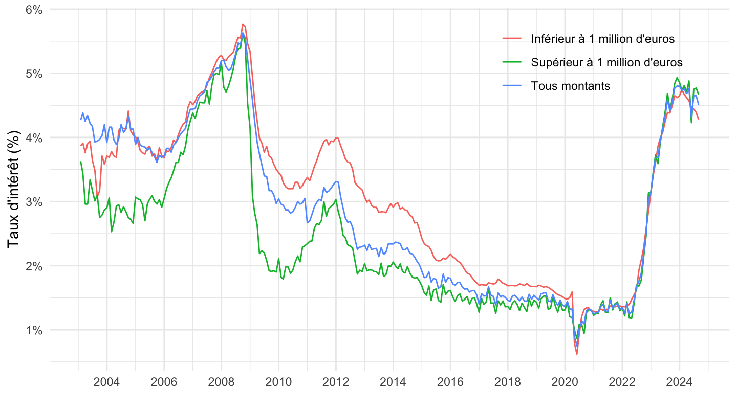
2010-
Code
MIR1 %>%
  filter(grepl("MIR1.M.FR.B.A20.A.R.0.2240U6.EUR.N", variable) |
           grepl("MIR1.M.FR.B.A20.A.R.1.2240U6.EUR.N", variable) |
           grepl("MIR1.M.FR.B.A20.A.R.A.2240U6.EUR.N", variable)) %>%


  arrange(desc(date)) %>%
  filter(date >= as.Date("2010-01-01")) %>%
  ggplot + geom_line(aes(x = date, y = value/100, color = Amount_cat)) +

  theme_minimal() +
  scale_x_date(breaks = as.Date(paste0(seq(1960, 2100, 2), "-01-01")),
               labels = date_format("%Y")) +
  theme(legend.position = c(0.7, 0.85),
        legend.title = element_blank(),
        legend.direction = "vertical") +
  xlab("") + ylab("Taux d'intérêt (%)") +
  scale_y_continuous(breaks = 0.01*seq(-10, 100, 0.5),
                labels = percent_format(accuracy = .1))
Catégories montants
Code
MIR1 %>%
  filter(grepl("MIR1.M.FR.B.A20.A.R.0.2240U6.EUR.N", variable) |
           grepl("MIR1.M.FR.B.A20.A.R.1.2240U6.EUR.N", variable) |
           grepl("MIR1.M.FR.B.A20.A.R.A.2240U6.EUR.N", variable)) %>%


  arrange(desc(date)) %>%
  ggplot + geom_line(aes(x = date, y = value/100, color = Amount_cat)) +

  theme_minimal() +
  scale_x_date(breaks = as.Date(paste0(seq(1960, 2100, 2), "-01-01")),
               labels = date_format("%Y")) +
  theme(legend.position = c(0.7, 0.85),
        legend.title = element_blank(),
        legend.direction = "vertical") +
  xlab("") + ylab("Taux d'intérêt (%)") +
  scale_y_continuous(breaks = 0.01*seq(-10, 100, 1),
                labels = percent_format(accuracy = 1))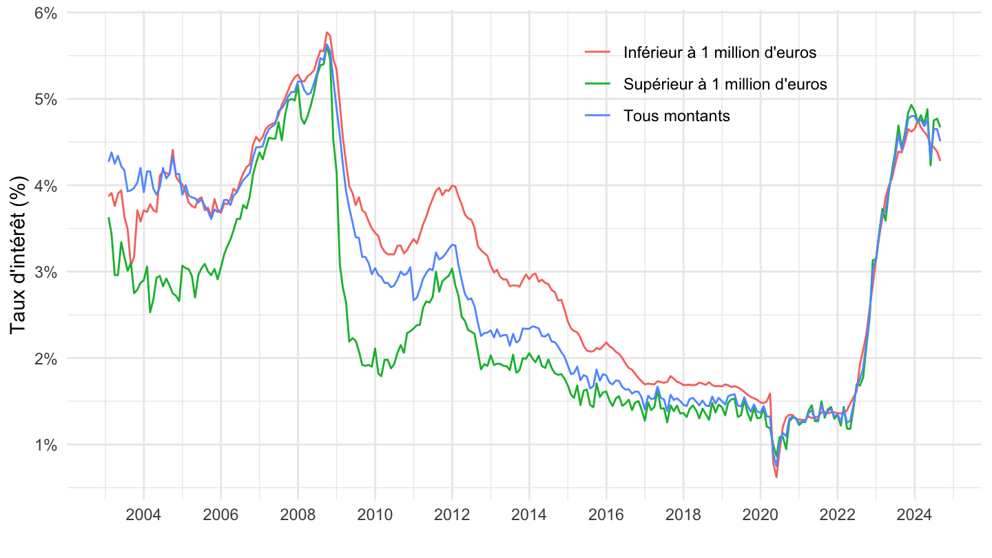
Livrets réglementés (avec LDDS)
Code
MIR1 %>%
  filter(grepl("MIR1.M.FR.B.L23FRLA.D.R.A.2230U6.EUR.O", variable) |
           grepl("MIR1.M.FR.B.L23RJ.A.R.A.2300.EUR.O", variable) |
           grepl("MIR1.M.FR.B.L23FRLJ.A.R.A.2250U6.EUR.O", variable) |
           grepl("MIR1.M.FR.B.L23FRLP.H.R.A.2250U6.EUR.O", variable) |
           grepl("MIR1.M.FR.B.L22FRSP.H.R.A.2250U6.EUR.N", variable)) %>%

  arrange(desc(date)) %>%
  ggplot + geom_line(aes(x = date, y = value/100, color = Variable)) +

  theme_minimal() +
  scale_x_date(breaks = as.Date(paste0(seq(1960, 2100, 5), "-01-01")),
               labels = date_format("%Y")) +
  theme(legend.position = c(0.4, 0.17),
        legend.title = element_blank(),
        legend.direction = "vertical") +
  xlab("") + ylab("Taux de rémunération annuel (%)") +
  scale_y_continuous(breaks = 0.01*seq(-10, 100, 1),
                labels = percent_format(accuracy = 1))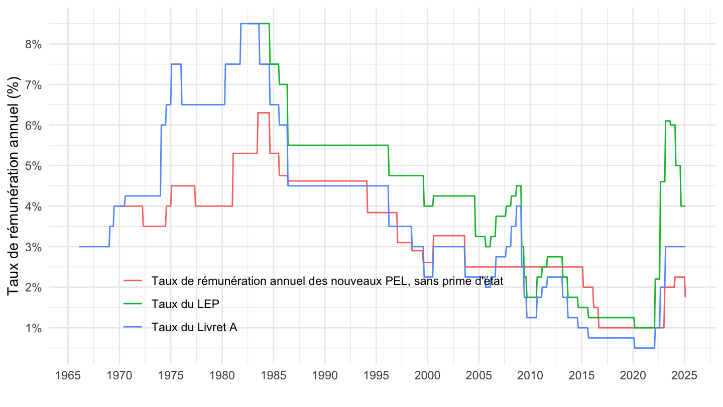
Livrets réglementés
Tous
Code
MIR1 %>%
  filter(grepl("MIR1.M.FR.B.L23FRLA.D.R.A.2230U6.EUR.O", variable) |
           grepl("MIR1.M.FR.B.L23RJ.A.R.A.2300.EUR.O", variable) |
           grepl("MIR1.M.FR.B.L23FRLJ.A.R.A.2250U6.EUR.O", variable) |
           grepl("MIR1.M.FR.B.L23FRLP.H.R.A.2250U6.EUR.O", variable) |
           grepl("MIR1.M.FR.B.L22FRSP.H.R.A.2250U6.EUR.N", variable)) %>%

  arrange(desc(date)) %>%
  ggplot + geom_line(aes(x = date, y = value/100, color = Variable)) +

  theme_minimal() +
  scale_x_date(breaks = as.Date(paste0(seq(1960, 2100, 5), "-01-01")),
               labels = date_format("%Y")) +
  theme(legend.position = c(0.4, 0.17),
        legend.title = element_blank(),
        legend.direction = "vertical") +
  xlab("") + ylab("Taux de rémunération annuel (%)") +
  scale_y_continuous(breaks = 0.01*seq(-10, 100, 1),
                labels = percent_format(accuracy = 1))
2000-
Code
MIR1 %>%
  filter(grepl("MIR1.M.FR.B.L23FRLA.D.R.A.2230U6.EUR.O", variable) |
           grepl("MIR1.M.FR.B.L23RJ.A.R.A.2300.EUR.O", variable) |
           grepl("MIR1.M.FR.B.L23FRLJ.A.R.A.2250U6.EUR.O", variable) |
           grepl("MIR1.M.FR.B.L23FRLP.H.R.A.2250U6.EUR.O", variable) |
           grepl("MIR1.M.FR.B.L22FRSP.H.R.A.2250U6.EUR.N", variable)) %>%

  arrange(desc(date)) %>%
  filter(date >= as.Date("2000-01-01")) %>%
  ggplot + geom_line(aes(x = date, y = value/100, color = Variable)) +

  theme_minimal() +
  scale_x_date(breaks = as.Date(paste0(seq(1960, 2100, 2), "-01-01")),
               labels = date_format("%Y")) +
  theme(legend.position = c(0.4, 0.85),
        legend.title = element_blank(),
        legend.direction = "vertical") +
  xlab("") + ylab("Taux de rémunération annuel (%)") +
  scale_y_continuous(breaks = 0.01*seq(-10, 100, 1),
                labels = percent_format(accuracy = 1))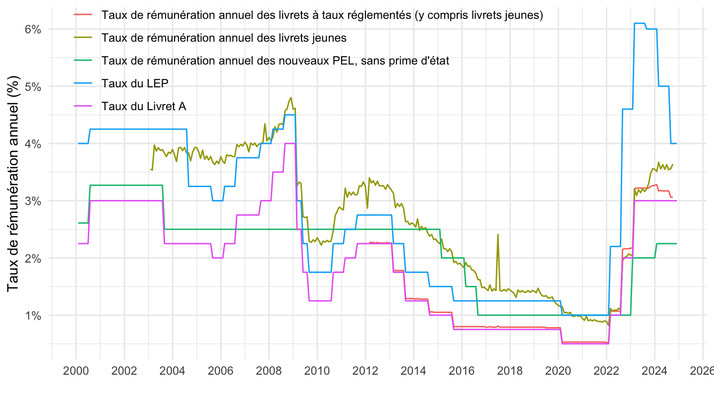
2010-
Code
MIR1 %>%
  filter(grepl("MIR1.M.FR.B.L23FRLA.D.R.A.2230U6.EUR.O", variable) |
           grepl("MIR1.M.FR.B.L23RJ.A.R.A.2300.EUR.O", variable) |
           grepl("MIR1.M.FR.B.L23FRLJ.A.R.A.2250U6.EUR.O", variable) |
           grepl("MIR1.M.FR.B.L23FRLP.H.R.A.2250U6.EUR.O", variable) |
           grepl("MIR1.M.FR.B.L22FRSP.H.R.A.2250U6.EUR.N", variable)) %>%

  arrange(desc(date)) %>%
  filter(date >= as.Date("2010-01-01")) %>%
  ggplot + geom_line(aes(x = date, y = value/100, color = Variable)) +

  theme_minimal() +
  scale_x_date(breaks = as.Date(paste0(seq(1960, 2100, 1), "-01-01")),
               labels = date_format("%Y")) +
  theme(legend.position = c(0.4, 0.8),
        legend.title = element_blank(),
        legend.direction = "vertical") +
  xlab("") + ylab("Taux de rémunération annuel (%)") +
  scale_y_continuous(breaks = 0.01*seq(-10, 100, 0.5),
                labels = percent_format(accuracy = .1))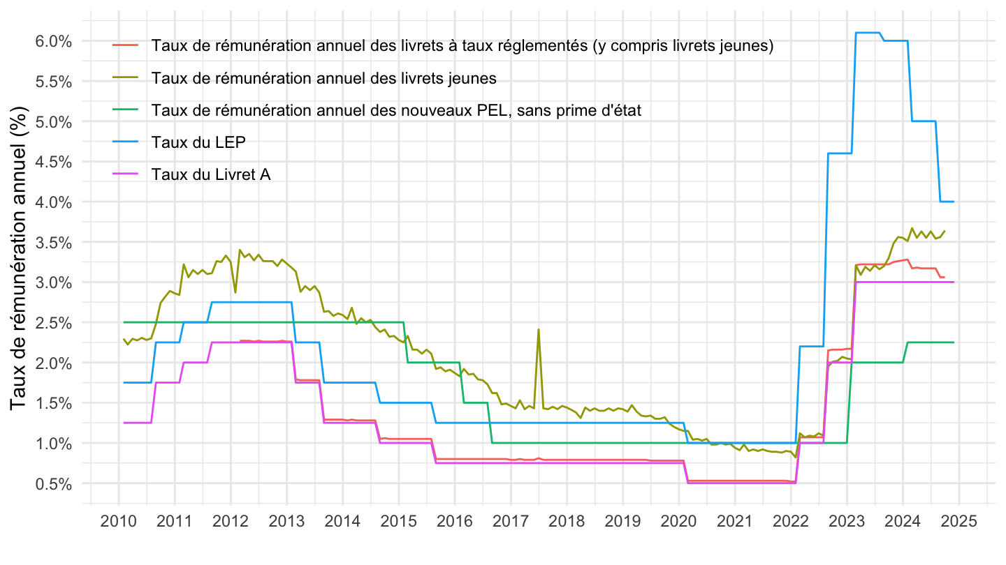
2018-
Code
MIR1 %>%
  filter(grepl("MIR1.M.FR.B.L23FRLA.D.R.A.2230U6.EUR.O", variable) |
           grepl("MIR1.M.FR.B.L23RJ.A.R.A.2300.EUR.O", variable) |
           grepl("MIR1.M.FR.B.L23FRLJ.A.R.A.2250U6.EUR.O", variable) |
           grepl("MIR1.M.FR.B.L23FRLP.H.R.A.2250U6.EUR.O", variable) |
           grepl("MIR1.M.FR.B.L22FRSP.H.R.A.2250U6.EUR.N", variable)) %>%

  arrange(desc(date)) %>%
  filter(date >= as.Date("2018-01-01")) %>%
  ggplot + geom_line(aes(x = date, y = value/100, color = Variable)) +

  theme_minimal() +
  scale_x_date(breaks = as.Date(paste0(seq(1960, 2100, 1), "-01-01")),
               labels = date_format("%Y")) +
  theme(legend.position = c(0.4, 0.8),
        legend.title = element_blank(),
        legend.direction = "vertical") +
  xlab("") + ylab("Taux de rémunération annuel (%)") +
  scale_y_continuous(breaks = 0.01*seq(-10, 100, 0.5),
                labels = percent_format(accuracy = .1))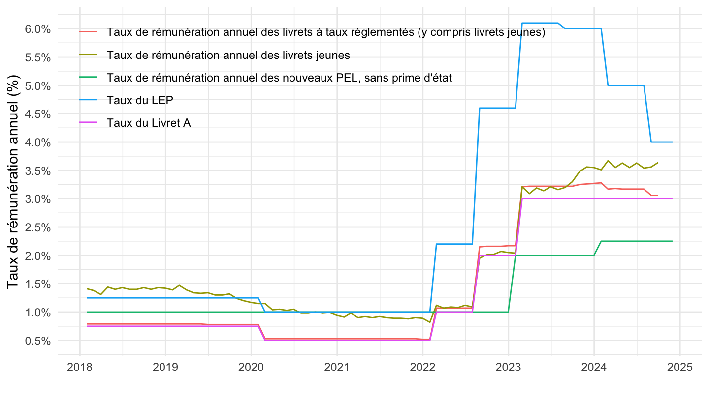
Taux crédits habitat
Tous
Code
# MIR1.M.FR.B.A22FRF.A.R.A.2254U6.EUR.N - Crédits nouveaux à l'habitat à taux fixe aux particuliers, taux d'intérêt, en %
# MIR1.M.FR.B.A22FRV.A.R.A.2254U6.EUR.N - Crédits nouveaux à l'habitat à taux variable aux particuliers, taux d'intérêt, en %
# MIR1.M.FR.B.A22HR.A.R.A.2254U6.EUR.N - Taux des crédits nouveaux à l'habitat (hors négociations) aux particuliers
MIR1 %>%

  filter(FREQ == "M",
         REF_AREA == "FR",
         BS_REP_SECTOR == "B",
         BS_ITEM == "A2C",
         DATA_TYPE_MIR == "R",
         AMOUNT_CAT == "A",
         BS_COUNT_SECTOR == "2250U6",
         CURRENCY_TRANS == "EUR",
         IR_BUS_COV == "N") %>%

  ggplot + geom_line(aes(x = date, y = value/100, color = Maturity_orig)) +

  theme_minimal() + xlab("") + ylab("Taux d'intérêt (%)") +
  scale_x_date(breaks = as.Date(paste0(seq(1960, 2100, 2), "-01-01")),
               labels = date_format("%Y")) +
  theme(legend.position = c(0.35, 0.15),
        legend.title = element_blank(),
        legend.direction = "vertical") +
  scale_y_continuous(breaks = 0.01*seq(-10, 100, 1),
                labels = percent_format(accuracy = 1))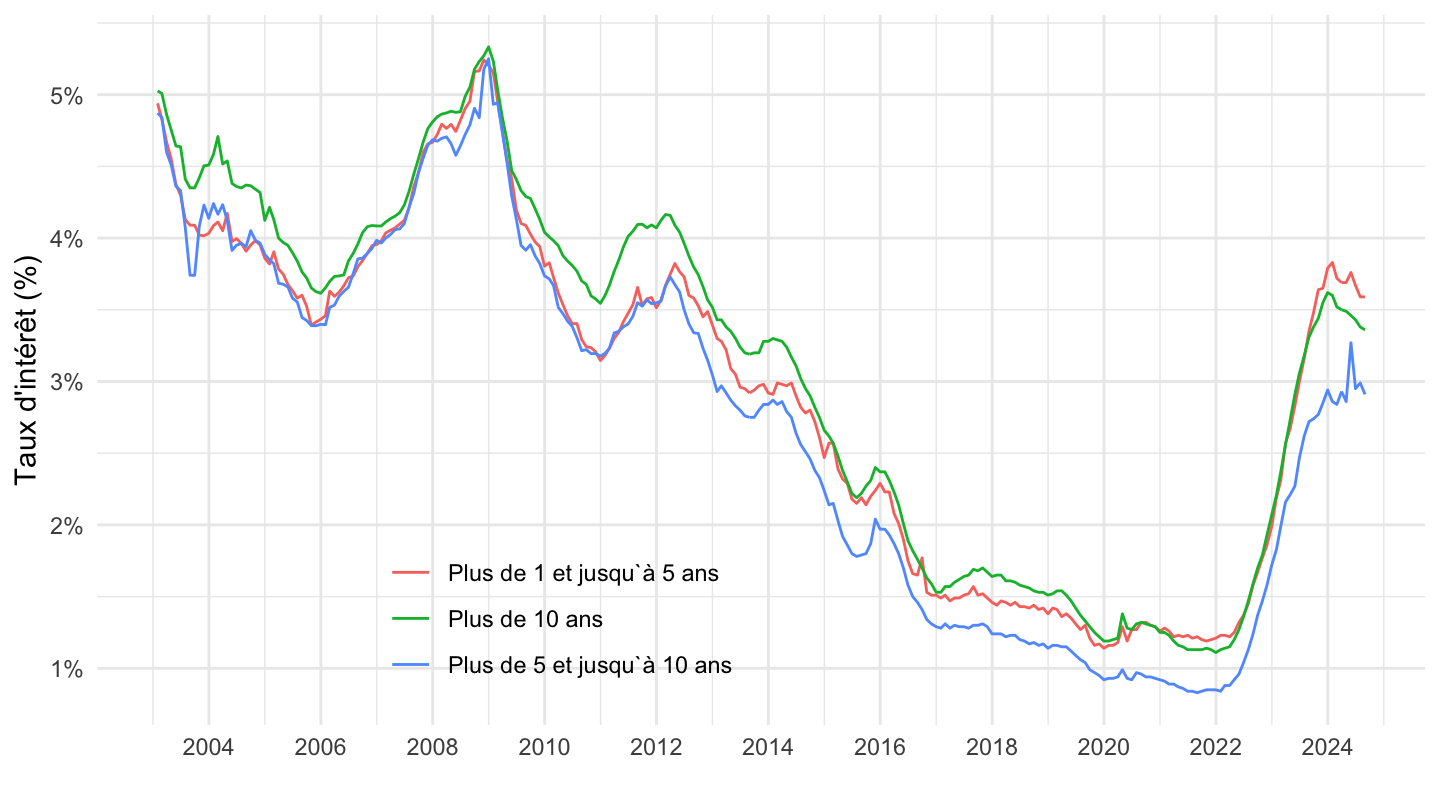
Tous
Code
MIR1 %>%
  filter(grepl("MIR1.M.FR.B.A22.K.R.A.2254U6.EUR.N", variable) |
           grepl("MIR1.M.FR.B.A22.F.R.A.2254U6.EUR.N", variable) |
           grepl("MIR1.M.FR.B.A22.A.R.A.2254U6.EUR.N", variable)) %>%

  ggplot + geom_line(aes(x = date, y = value/100, color = Variable)) +

  theme_minimal() +
  scale_x_date(breaks = as.Date(paste0(seq(1960, 2100, 2), "-01-01")),
               labels = date_format("%Y")) +
  theme(legend.position = c(0.35, 0.15),
        legend.title = element_blank(),
        legend.direction = "vertical") +
  xlab("") + ylab("Taux d'intérêt (%)") +
  scale_y_continuous(breaks = 0.01*seq(-10, 100, 1),
                labels = percent_format(accuracy = 1))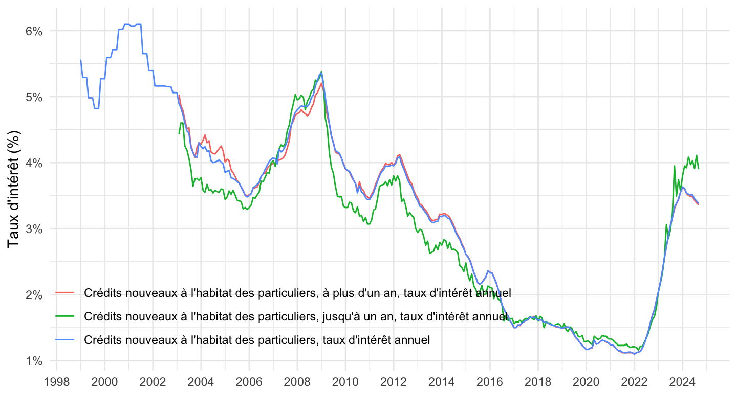
2016-
Code
MIR1 %>%
  filter(grepl("MIR1.M.FR.B.A22.K.R.A.2254U6.EUR.N", variable) |
           grepl("MIR1.M.FR.B.A22.F.R.A.2254U6.EUR.N", variable) |
           grepl("MIR1.M.FR.B.A22.A.R.A.2254U6.EUR.N", variable)) %>%

  filter(date >= as.Date("2016-01-01")) %>%
  ggplot + geom_line(aes(x = date, y = value/100, color = Variable)) +

  theme_minimal() +
  scale_x_date(breaks = as.Date(paste0(seq(1960, 2100, 1), "-01-01")),
               labels = date_format("%Y")) +
  theme(legend.position = c(0.4, 0.85),
        legend.title = element_blank(),
        legend.direction = "vertical") +
  xlab("") + ylab("Taux d'intérêt (%)") +
  scale_y_continuous(breaks = 0.01*seq(-10, 100, .1),
                labels = percent_format(accuracy = .1))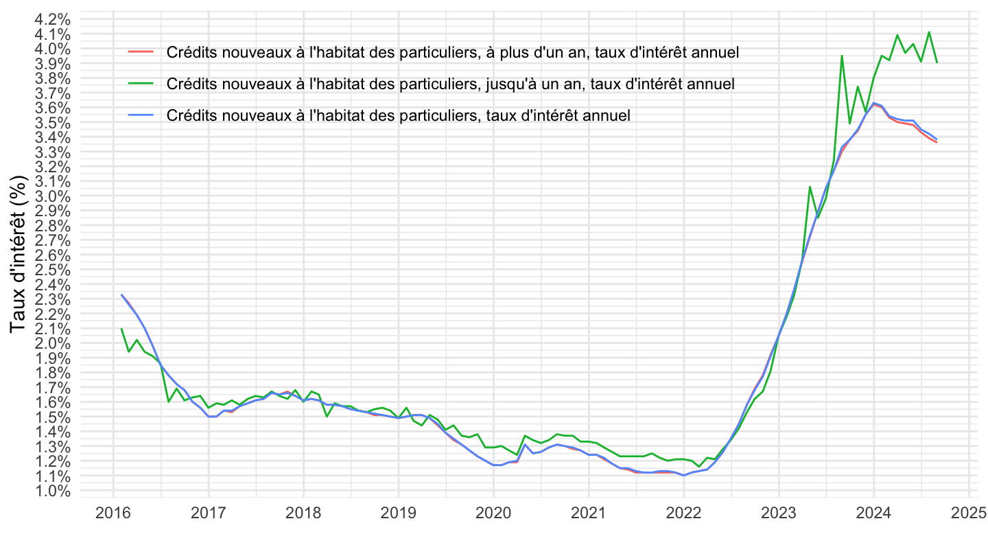
2018-
Code
MIR1 %>%
  filter(grepl("MIR1.M.FR.B.A22.K.R.A.2254U6.EUR.N", variable) |
           grepl("MIR1.M.FR.B.A22.F.R.A.2254U6.EUR.N", variable) |
           grepl("MIR1.M.FR.B.A22.A.R.A.2254U6.EUR.N", variable)) %>%

  filter(date >= as.Date("2018-01-01")) %>%
  ggplot + geom_line(aes(x = date, y = value/100, color = Variable)) +

  theme_minimal() +
  scale_x_date(breaks = as.Date(paste0(seq(1960, 2100, 1), "-01-01")),
               labels = date_format("%Y")) +
  theme(legend.position = c(0.4, 0.85),
        legend.title = element_blank(),
        legend.direction = "vertical") +
  xlab("") + ylab("Taux d'intérêt (%)") +
  scale_y_continuous(breaks = 0.01*seq(-10, 100, .1),
                labels = percent_format(accuracy = .1))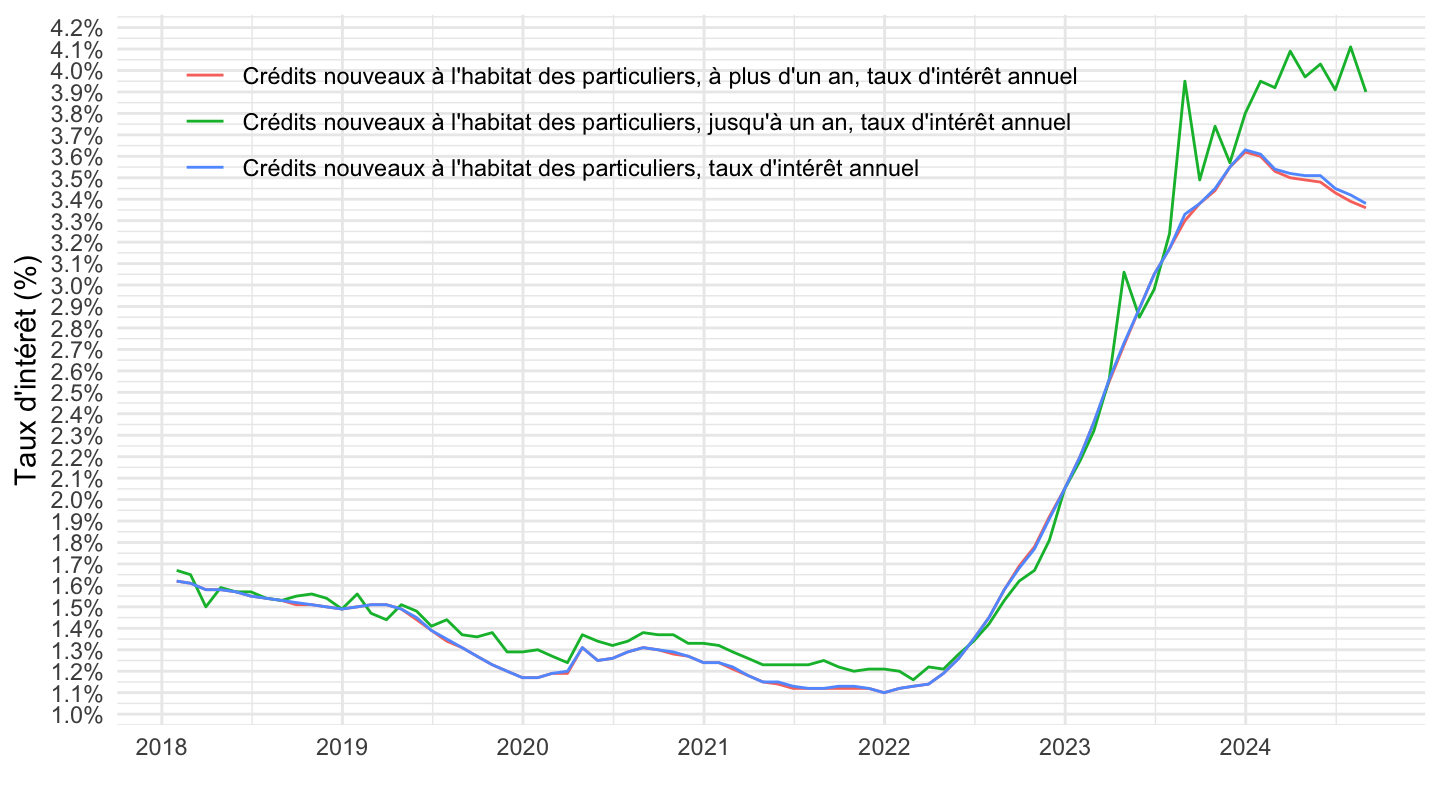
Taux de rémunération des dépôts + immobilier
Tous
Code
MIR1 %>%
  filter(grepl("MIR1.M.FR.A.N30.A.R.A.2230U6.EUR.O", variable) |
           grepl("MIR1.M.FR.B.A22.A.R.A.2254U6.EUR.N", variable) |
           grepl("MIR1.M.FR.B.L21.A.R.A.2230U6.EUR.O", variable)) %>%

  ggplot + geom_line(aes(x = date, y = value/100, color = Variable)) +

  theme_minimal() +
  scale_x_date(breaks = as.Date(paste0(seq(1960, 2100, 2), "-01-01")),
               labels = date_format("%Y")) +
  theme(legend.position = c(0.55, 0.9),
        legend.title = element_blank(),
        legend.direction = "vertical") +
  xlab("") + ylab("Taux d'intérêt (%)") +
  scale_y_continuous(breaks = 0.01*seq(-10, 100, 1),
                labels = percent_format(accuracy = 1),
                limits = c(0, 0.07))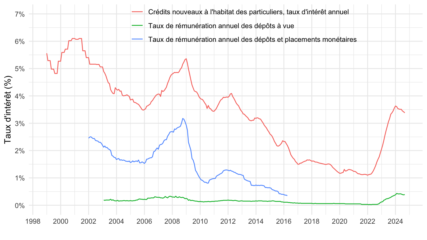
Part des renégociations
Code
MIR1 %>%
  filter(grepl("MIR1.M.FR.B.A22PR.A.W.A.2254FR.EUR.N", variable)) %>%

  na.omit %>%
  ggplot + geom_line(aes(x = date, y = value/100)) +
  theme_minimal() +
  scale_x_date(breaks = as.Date(paste0(seq(1960, 2100, 1), "-01-01")),
               labels = date_format("%Y")) +
  theme(legend.position = c(0.35, 0.15),
        legend.title = element_blank(),
        legend.direction = "vertical") +
  xlab("") + ylab("Part des renégo dans le total des crédits à l'habitat (%)") +
  scale_y_continuous(breaks = 0.01*seq(-10, 100, 5),
                labels = percent_format(accuracy = 1))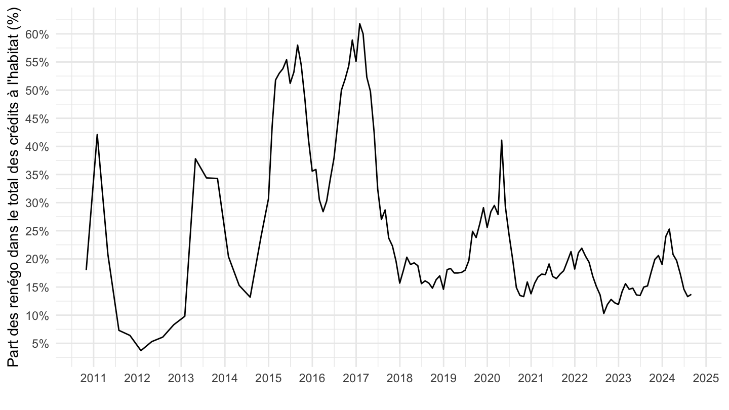
Volumes de crédit
Crédits à la consommation
Code
MIR1 %>%
  filter(grepl("MIR1.M.FR.B.A2Z.A.R.A.2254U6.EUR.N", variable) |
           grepl("MIR1.M.FR.B.A2B.A.R.A.2254U6.EUR.N", variable)) %>%

  ggplot + geom_line(aes(x = date, y = value/100, color = Variable)) +

  theme_minimal() +
  scale_x_date(breaks = as.Date(paste0(seq(1960, 2100, 2), "-01-01")),
               labels = date_format("%Y")) +
  theme(legend.position = c(0.5, 0.9),
        legend.title = element_blank(),
        legend.direction = "vertical") +
  xlab("") + ylab("Taux d'intérêt (%)") +
  scale_y_continuous(breaks = 0.01*seq(-10, 100, 1),
                labels = percent_format(accuracy = 1),
                limits = c(0.03, 0.15))
Crédits nouveaux à l’habitat
Tous
Code
MIR1 %>%
  filter(grepl("MIR1.M.FR.B.A22HR.A.5.A.2254U6.EUR.N", variable) |
           grepl("MIR1.M.FR.B.A22.A.5.A.2254U6.EUR.N", variable)) %>%

  ggplot + geom_line(aes(x = date, y = value, color = Variable)) +

  theme_minimal() +
  scale_x_date(breaks = as.Date(paste0(seq(1960, 2100, 2), "-01-01")),
               labels = date_format("%Y")) +
  theme(legend.position = c(0.5, 0.9),
        legend.title = element_blank(),
        legend.direction = "vertical") +
  xlab("") + ylab("") +
  scale_y_continuous(breaks = seq(0, 100, 2))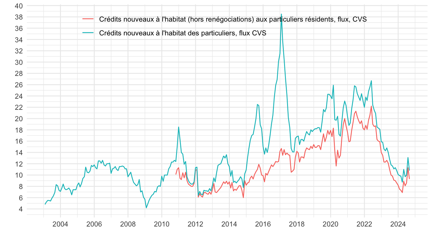
2015-
Code
MIR1 %>%
  filter(grepl("MIR1.M.FR.B.A22HR.A.5.A.2254U6.EUR.N", variable) |
           grepl("MIR1.M.FR.B.A22.A.5.A.2254U6.EUR.N", variable)) %>%

  filter(date >= as.Date("2015-01-01")) %>%
  ggplot + geom_line(aes(x = date, y = value, color = Variable)) +

  theme_minimal() +
  scale_x_date(breaks = as.Date(paste0(seq(1960, 2100, 1), "-01-01")),
               labels = date_format("%Y")) +
  theme(legend.position = c(0.5, 0.9),
        legend.title = element_blank(),
        legend.direction = "vertical") +
  xlab("") + ylab("") +
  scale_y_continuous(breaks = seq(0, 100, 2))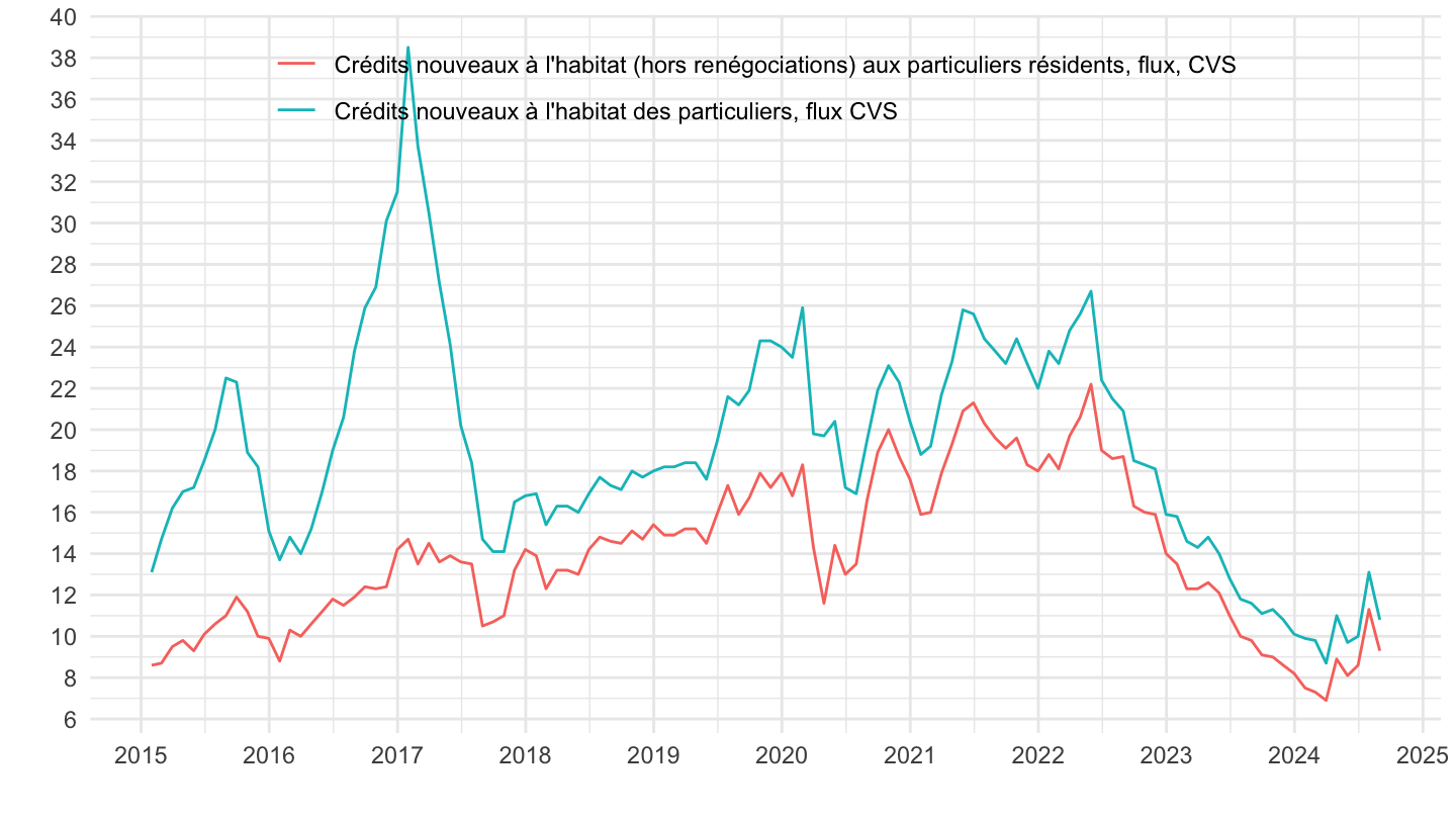
Taux d’usure
2017-
Code
MIR1 %>%
  filter(grepl("MIR1.Q.FR.R.A22FRF.Q.U.A.2254FR.EUR.N", variable) |
           grepl("MIR1.Q.FR.R.A22FRF.R.U.A.2254FR.EUR.N", variable) |
           grepl("MIR1.Q.FR.R.A22FRF.S.U.A.2254FR.EUR.N", variable)) %>%

  ggplot + geom_line(aes(x = date, y = value/100, color = Variable)) +
  theme_minimal() +
  scale_x_date(breaks = as.Date(paste0(seq(1960, 2100, 1), "-01-01")),
               labels = date_format("%Y")) +
  theme(legend.position = c(0.5, 0.9),
        legend.title = element_blank(),
        legend.direction = "vertical") +
  xlab("") + ylab("Taux d'intérêt (%)") +
  scale_y_continuous(breaks = 0.01*seq(-10, 100, 0.1),
                labels = percent_format(accuracy = .1))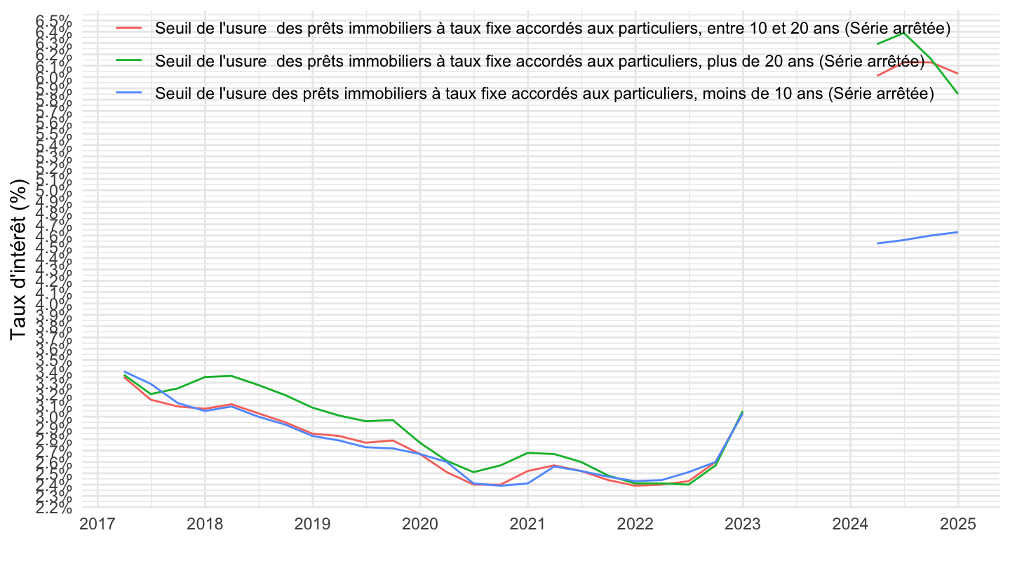
Pour en savoir plus…
Données sur les taux d’intérêt
| source | dataset | Title | .html | .rData |
|---|---|---|---|---|
| bdf | MIR | Taux d'intérêt - Zone euro | 2026-07-22 | 2026-07-22 |
| bdf | FM | Marché financier, taux | 2026-07-22 | 2026-07-22 |
| bdf | MIR1 | Taux d'intérêt - France | 2026-07-23 | 2026-07-23 |
| bis | CBPOL_D | Policy Rates, Daily | 2026-07-18 | 2025-08-20 |
| bis | CBPOL_M | Policy Rates, Monthly | 2026-07-22 | 2024-04-19 |
| ecb | FM | Financial market data | 2026-07-23 | 2026-07-22 |
| ecb | MIR | MFI Interest Rate Statistics | 2026-07-23 | 2026-07-22 |
Données sur l’immobilier
| source | dataset | Title | .html | .rData |
|---|---|---|---|---|
| bdf | MIR | Taux d'intérêt - Zone euro | 2026-07-22 | 2026-07-22 |
| acpr | as151 | Enquête annuelle du SGACPR sur le financement de l'habitat 2022 | 2026-07-22 | 2024-04-05 |
| acpr | as160 | Enquête annuelle du SGACPR sur le financement de l'habitat 2023 | 2026-07-22 | 2024-09-26 |
| acpr | as174 | Enquête annuelle du SGACPR sur le financement de l'habitat 2024 | 2026-07-22 | 2025-09-29 |
| bdf | BSI1 | Agrégats monétaires - France | 2026-07-22 | 2026-07-22 |
| bdf | CPP | Prix immobilier commercial | 2026-07-22 | 2024-07-01 |
| bdf | FM | Marché financier, taux | 2026-07-22 | 2026-07-22 |
| bdf | MIR1 | Taux d'intérêt - France | 2026-07-23 | 2026-07-23 |
| bdf | RPP | Prix de l'immobilier | 2026-07-22 | 2026-07-22 |
| bdf | immobilier | Immobilier en France | 2026-07-22 | 2026-07-21 |
| cgedd | nombre-vente-maison-appartement-ancien | Nombre de ventes de logements anciens cumulé sur 12 mois | 2026-07-22 | 2026-07-22 |
| insee | CONSTRUCTION-LOGEMENTS | Construction de logements | 2026-07-23 | 2026-07-23 |
| insee | ENQ-CONJ-ART-BAT | Conjoncture dans l'artisanat du bâtiment | 2026-07-23 | 2026-07-23 |
| insee | ENQ-CONJ-IND-BAT | Conjoncture dans l'industrie du bâtiment - ENQ-CONJ-IND-BAT | 2026-07-23 | 2026-07-23 |
| insee | ENQ-CONJ-PROMO-IMMO | Conjoncture dans la promotion immobilière | 2026-07-23 | 2026-07-23 |
| insee | ENQ-CONJ-TP | Conjoncture dans les travaux publics | 2026-07-23 | 2026-07-23 |
| insee | ILC-ILAT-ICC | Indices pour la révision d’un bail commercial ou professionnel | 2026-07-23 | 2026-07-23 |
| insee | INDICES_LOYERS | Indices des loyers d'habitation (ILH) | 2026-07-23 | 2026-07-23 |
| insee | IPLA-IPLNA-2015 | Indices des prix des logements neufs et Indices Notaires-Insee des prix des logements anciens | 2026-07-23 | 2026-07-23 |
| insee | IRL | Indice pour la révision d’un loyer d’habitation | 2026-07-23 | 2026-07-23 |
| insee | PARC-LOGEMENTS | Estimations annuelles du parc de logements (EAPL) | 2026-07-23 | 2026-07-23 |
| insee | SERIES_LOYERS | Variation des loyers | 2026-07-23 | 2026-07-23 |
| insee | t_dpe_val | Dépenses de consommation des ménages pré-engagées | 2026-07-23 | 2026-02-27 |
| notaires | arrdt | Prix au m^2 par arrondissement - arrdt | 2026-07-22 | 2026-07-22 |
| notaires | dep | Prix au m^2 par département | 2026-07-22 | 2026-07-22 |
| olap | loyers | Loyers | 2024-06-20 | 2023-07-20 |