Immobilier en France - immobilier

Name: Immobilier en France
Creator: François Geerolf
License: https://www.etalab.gouv.fr/licence-ouverte-open-licence/

Données - BDF

Auteur

François Geerolf

🇬🇧 English version

variable

Code

immobilier |>
  left_join(variable, by = "variable") |>
  group_by(variable, Variable) |>
  summarise(Nobs = n(),
            max_date = max(date),
            min_date = min(date)) |>
  arrange(desc(max_date)) |>
  print_table_conditional()

variable	Variable	Nobs	max_date	min_date
FM.D.U2.EUR.4F.KR.DFR.LEV	BCE - Facilité de dépôt (données brutes)	10064	2026-07-21	1999-01-01
BSI1.M.FR.N.R.A220Z.A.1.U6.2254FR.Z01.E	Crédits à l'habitat accordés aux particuliers résidents, encours	398	2026-05-31	1993-04-30
BSI1.M.FR.N.R.A26.A.1.U6.2254FR.Z01.E	Crédits accordés aux particuliers résidents, encours	398	2026-05-31	1993-04-30
BSI1.M.FR.Y.R.A220Z.A.4.U6.2254FR.Z01.E	Crédits à l'habitat accordés aux particuliers résidents, flux mensuels, CVS	398	2026-05-31	1993-04-30
BSI1.M.FR.Y.R.A220Z.A.4.U6.2254FR.Z01.V3F	Crédits à l'habitat accordés aux particuliers résidents, variation d'encours (moyenne sur 3 mois glissants), CVS	398	2026-05-31	1993-04-30
MIR1.M.FR.B.A22.A.5.A.2254U6.EUR.N	Crédits nouveaux à l'habitat des particuliers, flux CVS	281	2026-05-31	2003-01-31
MIR1.M.FR.B.A22.A.R.A.2254U6.EUR.N	Crédits nouveaux à l'habitat des particuliers, taux d'intérêt annuel	330	2026-05-31	1998-12-31
MIR1.M.FR.B.A22HR.A.5.A.2254U6.EUR.N	Crédits nouveaux à l'habitat (hors renégociations) aux particuliers résidents, flux, CVS	281	2026-05-31	2003-01-31
FM.M.U2.EUR.4F.KR.DF.LEV	BCE - Facilité de dépôt - niveau fin de mois yc mois en cours	290	2023-02-28	1999-01-31
FM.M.U2.EUR.4F.KR.MLF.LEV	BCE - Facilité de prêt marginal - niveau fin de mois yc mois en cours	290	2023-02-28	1999-01-31
FM.M.U2.EUR.4F.KR.MRR_FR.LEV	BCE - Principales opérations de refinancement (taux fixe)	290	2023-02-28	1999-01-31

Comparer taux crédits immobilier et taux banque centrale

Tous

1 année

Code

immobilier |>
  filter(variable == "MIR1.M.FR.B.A22.A.R.A.2254U6.EUR.N" |
           variable == "FM.D.U2.EUR.4F.KR.DFR.LEV") |>
  left_join(variable, by = "variable") |>
  ggplot() + geom_line(aes(x = date, y = value/100, color = Variable)) +
  theme_minimal() + xlab("") + ylab("Taux d'intérêt (%)") +
  theme(legend.position = c(0.32, 0.1),
        legend.title = element_blank()) +
  scale_x_date(breaks = as.Date(paste0(seq(1960, 2100, 2), "-01-01")),
               labels = date_format("%Y")) +
  scale_y_continuous(breaks = 0.01*seq(-10, 100, 1),
                labels = percent_format(accuracy = 1))

2 ans

Tous

Code

immobilier |>
  filter(variable == "MIR1.M.FR.B.A22.A.R.A.2254U6.EUR.N" |
           variable == "FM.D.U2.EUR.4F.KR.DFR.LEV") |>
  left_join(variable, by = "variable") |>
  ggplot() + geom_line(aes(x = date, y = value/100, color = Variable)) +
  theme_minimal() + xlab("") + ylab("Taux d'intérêt (%)") +
  theme(legend.position = c(0.32, 0.1),
        legend.title = element_blank()) +
  scale_x_date(breaks = as.Date(paste0(seq(1960, 2100, 2), "-01-01")),
               labels = date_format("%Y")) +
  scale_y_continuous(breaks = 0.01*seq(-10, 100, 0.5),
                labels = percent_format(accuracy = .1))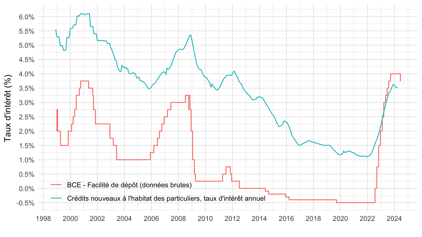

2020-

Code

immobilier |>
  filter(variable == "MIR1.M.FR.B.A22.A.R.A.2254U6.EUR.N" |
           variable == "FM.D.U2.EUR.4F.KR.DFR.LEV") |>
  left_join(variable, by = "variable") |>
  filter(date >= as.Date("2020-01-01")) |>
  ggplot() + geom_line(aes(x = date, y = value/100, color = Variable)) +
  theme_minimal() + xlab("") + ylab("Taux d'intérêt (%)") +
  theme(legend.position = c(0.35, 0.9),
        legend.title = element_blank(),
        axis.text.x = element_text(angle = 45, vjust = 1, hjust = 1)) +
  scale_x_date(breaks = "3 months",
               labels = date_format("%b %Y")) +
  scale_y_continuous(breaks = 0.01*seq(-10, 100, .25),
                labels = percent_format(accuracy = .01))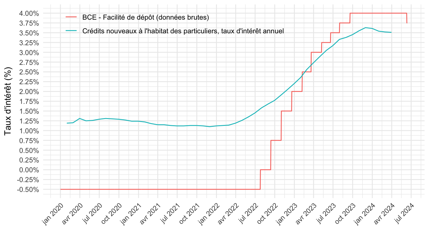

2021-

Code

immobilier |>
  filter(variable == "MIR1.M.FR.B.A22.A.R.A.2254U6.EUR.N" |
           variable == "FM.D.U2.EUR.4F.KR.DFR.LEV") |>
  left_join(variable, by = "variable") |>
  filter(date >= as.Date("2021-01-01")) |>
  ggplot() + geom_line(aes(x = date, y = value/100, color = Variable)) +
  #scale_color_manual(values = viridis(3)[1:2]) +
  theme_minimal() + xlab("") + ylab("Taux d'intérêt (%)") +
  theme(legend.position = c(0.35, 0.9),
        legend.title = element_blank(),
        axis.text.x = element_text(angle = 45, vjust = 1, hjust = 1)) +
  scale_x_date(breaks = "2 months",
               labels = date_format("%b %Y")) +
  scale_y_continuous(breaks = 0.01*seq(-10, 100, .25),
                labels = percent_format(accuracy = .01))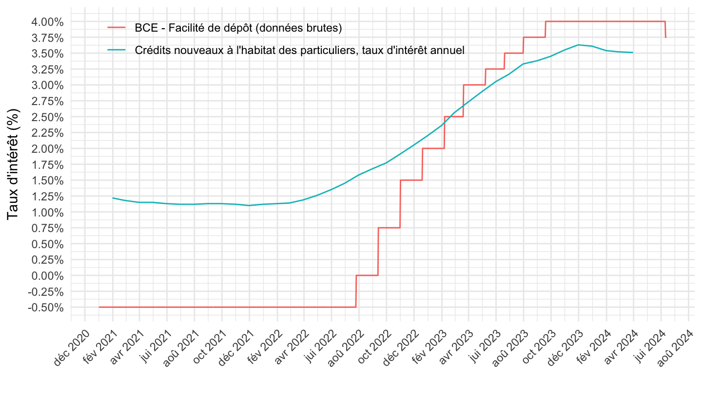

2022-

Code

immobilier |>
  filter(variable == "MIR1.M.FR.B.A22.A.R.A.2254U6.EUR.N" |
           variable == "FM.D.U2.EUR.4F.KR.DFR.LEV") |>
  left_join(variable, by = "variable") |>
  filter(date >= as.Date("2022-01-01")) |>
  ggplot() + geom_line(aes(x = date, y = value/100, color = Variable)) +
  #scale_color_manual(values = viridis(3)[1:2]) +
  theme_minimal() + xlab("") + ylab("Taux d'intérêt (%)") +
  theme(legend.position = c(0.35, 0.9),
        legend.title = element_blank(),
        axis.text.x = element_text(angle = 45, vjust = 1, hjust = 1)) +
  scale_x_date(breaks = "1 month",
               labels = date_format("%b %Y")) +
  scale_y_continuous(breaks = 0.01*seq(-10, 100, .25),
                labels = percent_format(accuracy = .01))

Tous les taux

Code

immobilier |>
  filter(variable == "MIR1.M.FR.B.A22.A.R.A.2254U6.EUR.N" |
           variable == "FM.M.U2.EUR.4F.KR.MRR_FR.LEV" |
           variable == "FM.M.U2.EUR.4F.KR.MLF.LEV" |
           variable == "FM.D.U2.EUR.4F.KR.DFR.LEV") |>
  left_join(variable, by = "variable") |>
  ggplot() + geom_line(aes(x = date, y = value/100, color = Variable, linetype = Variable)) +
  scale_color_manual(values = c(viridis(3)[1], viridis(3)[1], viridis(3)[1], viridis(3)[2])) +
  scale_linetype_manual(values = c("dashed", "longdash", "solid", "solid")) +
  theme_minimal() + xlab("") + ylab("Taux d'intérêt (%)") +
  theme(legend.position = c(0.32, 0.13),
        legend.title = element_blank(), 
        legend.spacing.x = unit(0.2, 'cm'),
        legend.spacing.y = unit(0.2, 'cm')) +
  scale_x_date(breaks = as.Date(paste0(seq(1960, 2100, 2), "-01-01")),
               labels = date_format("%Y")) +
  scale_y_continuous(breaks = 0.01*seq(-10, 100, 1),
                labels = percent_format(accuracy = 1),
                limits = c(-0.02, 0.065))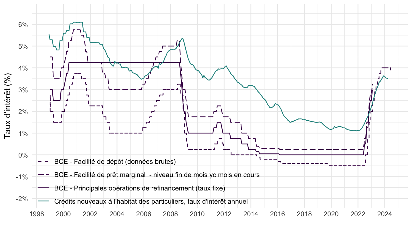

Crédits à l’habitat

Encours

Linear

Code

plot_linear <- immobilier |>
  filter(variable == "BSI1.M.FR.N.R.A26.A.1.U6.2254FR.Z01.E" |
           variable == "BSI1.M.FR.N.R.A220Z.A.1.U6.2254FR.Z01.E") |>
  left_join(variable, by = "variable") |>
  ggplot() + theme_minimal() + xlab("") + ylab("") +
  geom_line(aes(x = date, y = value / 1000, color = Variable)) +
  
  scale_x_date(breaks = as.Date(paste0(seq(1960, 2100, 5), "-01-01")),
               labels = date_format("%Y")) +
  theme(legend.position = c(0.4, 0.9),
        legend.title = element_blank(),
        legend.direction = "vertical") +
  scale_y_continuous(breaks = seq(-10000, 10000, 100),
                labels = dollar_format(suffix = " Mds€", prefix = "",  accuracy = 1))

plot_linear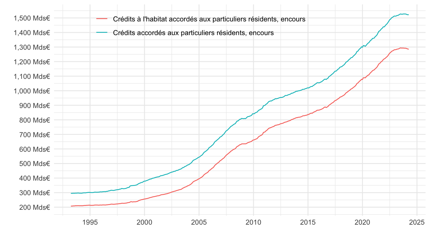

Log

Code

plot_log <- plot_linear +
  scale_y_log10(breaks = seq(-10000, 10000, 100),
                     labels = dollar_format(suffix = " Mds€", prefix = "",  accuracy = 1))

plot_log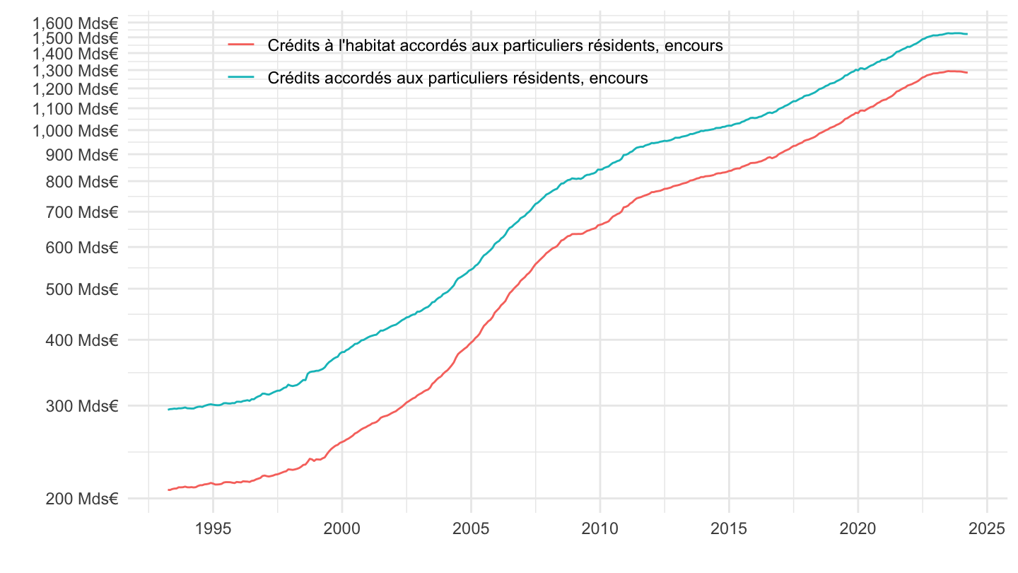

Both

Code

library("ggpubr")
ggarrange(plot_linear + ggtitle("Linear"), plot_log + ggtitle("Log"), common.legend = T, legend = "bottom")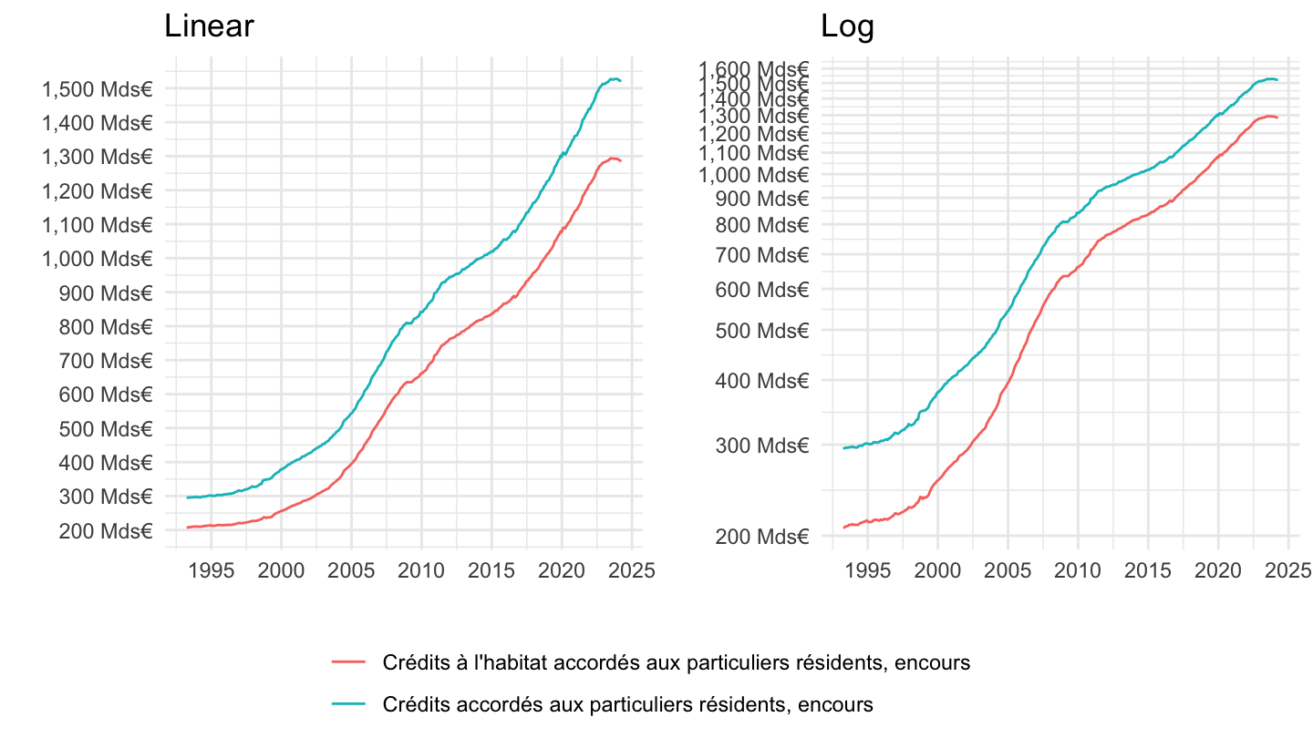

Montants mensuels

All

Code

immobilier |>
  filter(variable == "BSI1.M.FR.Y.R.A220Z.A.4.U6.2254FR.Z01.E") |>
  na.omit() |>
  ggplot() + geom_line(aes(x = date, y = value)) +
  theme_minimal() + xlab("") + ylab("") +
  scale_x_date(breaks = as.Date(paste0(seq(1960, 2100, 2), "-01-01")),
               labels = date_format("%Y")) +
  scale_y_continuous(breaks = seq(-10000, 10000, 1000))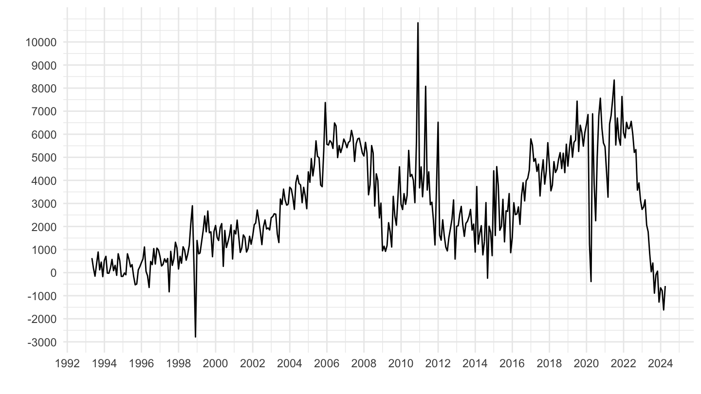

2000-

Code

immobilier |>
  filter(variable == "BSI1.M.FR.Y.R.A220Z.A.4.U6.2254FR.Z01.E",
         date >= as.Date("1999-12-31")) |>
  na.omit() |>
  ggplot() + geom_line(aes(x = date, y = value)) +
  theme_minimal() + xlab("") + ylab("") +
  scale_x_date(breaks = as.Date(paste0(seq(1960, 2100, 2), "-01-01")),
               labels = date_format("%Y")) +
  scale_y_continuous(breaks = seq(-10000, 10000, 1000))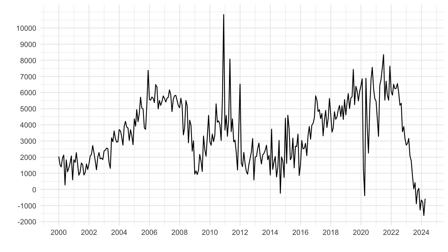

3 mois

All

Code

immobilier |>
  filter(variable == "BSI1.M.FR.Y.R.A220Z.A.4.U6.2254FR.Z01.V3F") |>
  na.omit() |>
  ggplot() + geom_line(aes(x = date, y = value)) +
  theme_minimal() + xlab("") + ylab("Crédits à l'habitat accordés aux particuliers résidents\n variation d'encours (moyenne sur 3 mois glissants)") +
  theme(axis.text.x = element_text(angle = 45, vjust = 1, hjust = 1)) +
  scale_x_date(breaks = as.Date(paste0(seq(1960, 2100, 1), "-01-01")),
               labels = date_format("%Y")) +
  scale_y_continuous(breaks = seq(-10000, 10000, 1000),
                     labels = dollar_format(acc = 1, pre = ""))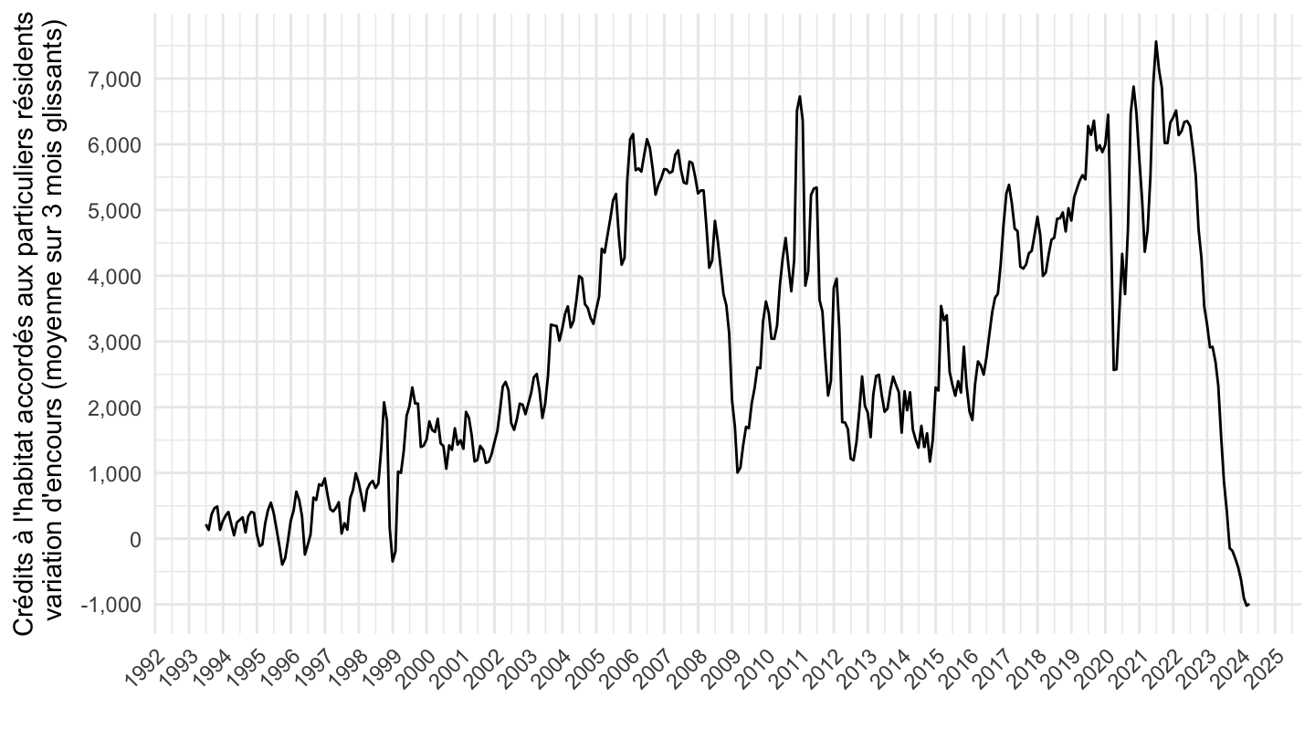

2000-

Code

immobilier |>
  filter(variable == "BSI1.M.FR.Y.R.A220Z.A.4.U6.2254FR.Z01.V3F") |>
  na.omit() |>
  ggplot() + geom_line(aes(x = date, y = value/1000)) +
  theme_minimal() + xlab("") + ylab("Crédits à l'habitat accordés aux particuliers résidents\n variation d'encours (moyenne sur 3 mois glissants)") +
  theme(axis.text.x = element_text(angle = 45, vjust = 1, hjust = 1)) +
  scale_x_date(breaks = as.Date(paste0(seq(1960, 2100, 1), "-01-01")),
               labels = date_format("%Y")) +
  scale_y_continuous(breaks = seq(-10000, 10000, 1000)/1000,
                     labels = dollar_format(acc = 1, pre = "", su = " Mds€"))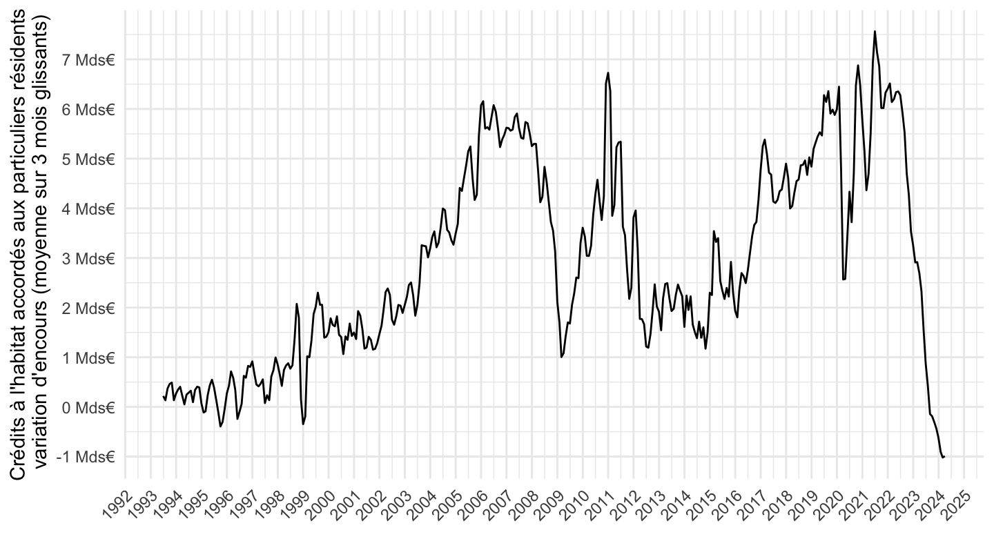

Last year

Code

immobilier |>
  filter(date >= Sys.Date() - months(18)) |>
  filter(variable == "BSI1.M.FR.Y.R.A220Z.A.4.U6.2254FR.Z01.V3F") |>
  na.omit() |>
  ggplot() + geom_line(aes(x = date, y = value)) +
  theme_minimal() + xlab("") + ylab("") +
  theme(axis.text.x = element_text(angle = 45, vjust = 1, hjust = 1)) +
  scale_x_date(breaks = "1 month",
               labels = date_format("%b %Y")) +
  scale_y_continuous(breaks = seq(-10000, 10000, 1000),
                     labels = dollar_format(acc = 1, pre = ""))

1 mois, 3 mois

Code

immobilier |>
  filter(variable == "BSI1.M.FR.Y.R.A220Z.A.4.U6.2254FR.Z01.V3F" |
           variable == "BSI1.M.FR.Y.R.A220Z.A.4.U6.2254FR.Z01.E") |>
  left_join(variable, by = "variable") |>
  ggplot() + geom_line(aes(x = date, y = value, color = Variable)) +
  theme_minimal() + xlab("") + ylab("") +
  theme(legend.position = c(0.5, 0.9),
        legend.title = element_blank()) +
  scale_x_date(breaks = as.Date(paste0(seq(1960, 2100, 2), "-01-01")),
               labels = date_format("%Y")) +
  scale_y_continuous(breaks = seq(-10000, 10000, 1000))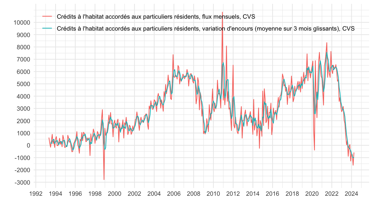

Crédits nouveaux à l’habitat (hors renégociation)

All

Code

immobilier |>
  filter(variable == "MIR1.M.FR.B.A22HR.A.5.A.2254U6.EUR.N" |
           variable == "MIR1.M.FR.B.A22.A.5.A.2254U6.EUR.N") |>
  left_join(variable, by = "variable") |>
  ggplot() + geom_line(aes(x = date, y = value, color = Variable)) +
  theme_minimal() + xlab("") + ylab("") +
  theme(legend.position = c(0.4, 0.9),
        legend.title = element_blank()) +
  scale_x_date(breaks = as.Date(paste0(seq(1960, 2100, 2), "-01-01")),
               labels = date_format("%Y")) +
  scale_y_continuous(breaks = seq(-100, 100, 5))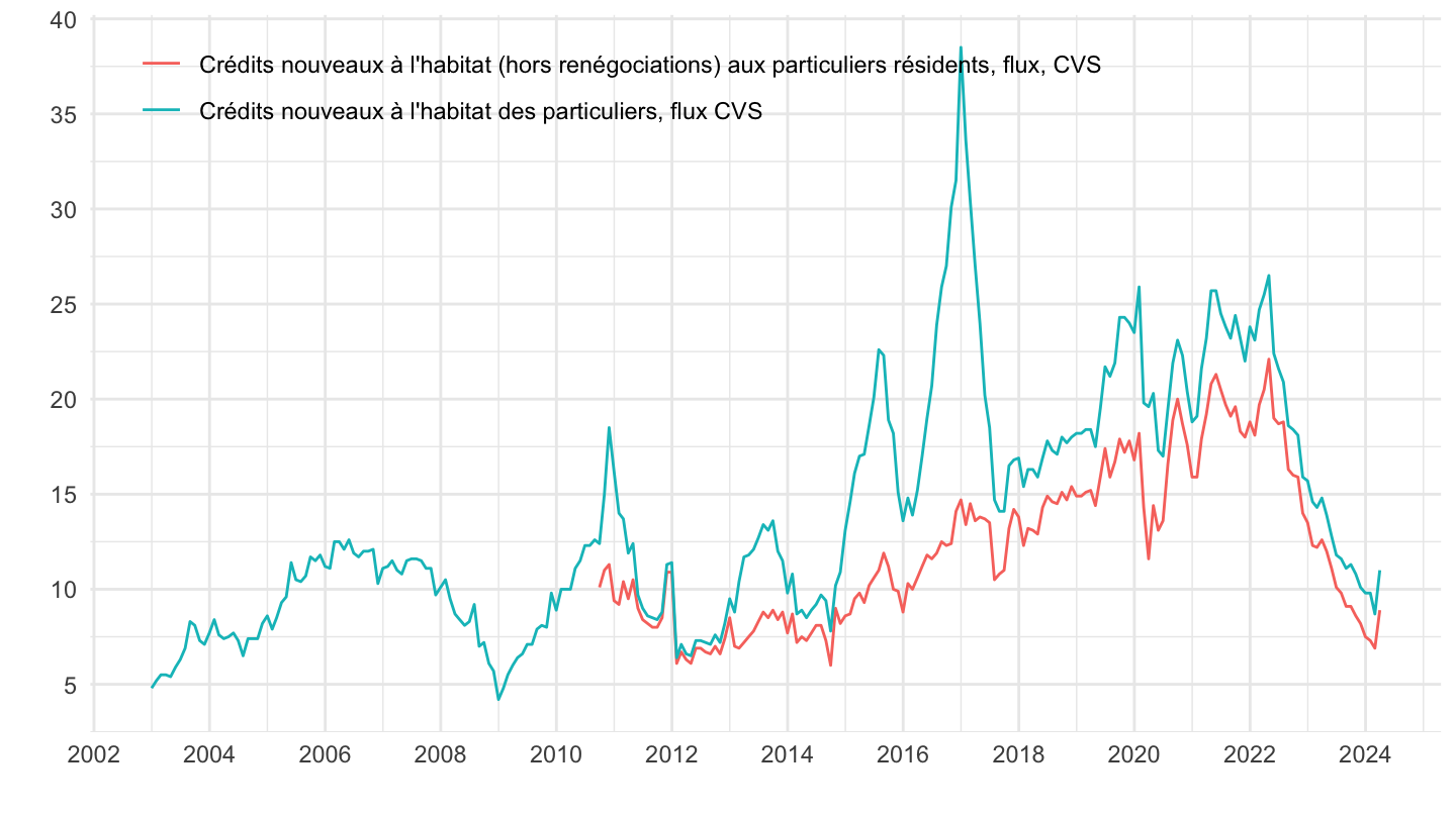

Complete series

Code

immobilier |>
  filter(variable == "MIR1.M.FR.B.A22HR.A.5.A.2254U6.EUR.N" |
           variable == "MIR1.M.FR.B.A22.A.5.A.2254U6.EUR.N") |>
  left_join(variable, by = "variable") |>
  group_by(date) |>
  filter(n() == 2) |>
  ggplot() + geom_line(aes(x = date, y = value, color = Variable)) +
  theme_minimal() + xlab("") + ylab("") +
  theme(legend.position = c(0.4, 0.9),
        legend.title = element_blank()) +
  scale_x_date(breaks = as.Date(paste0(seq(1960, 2100, 1), "-01-01")),
               labels = date_format("%Y")) +
  scale_y_continuous(breaks = seq(-100, 100, 5))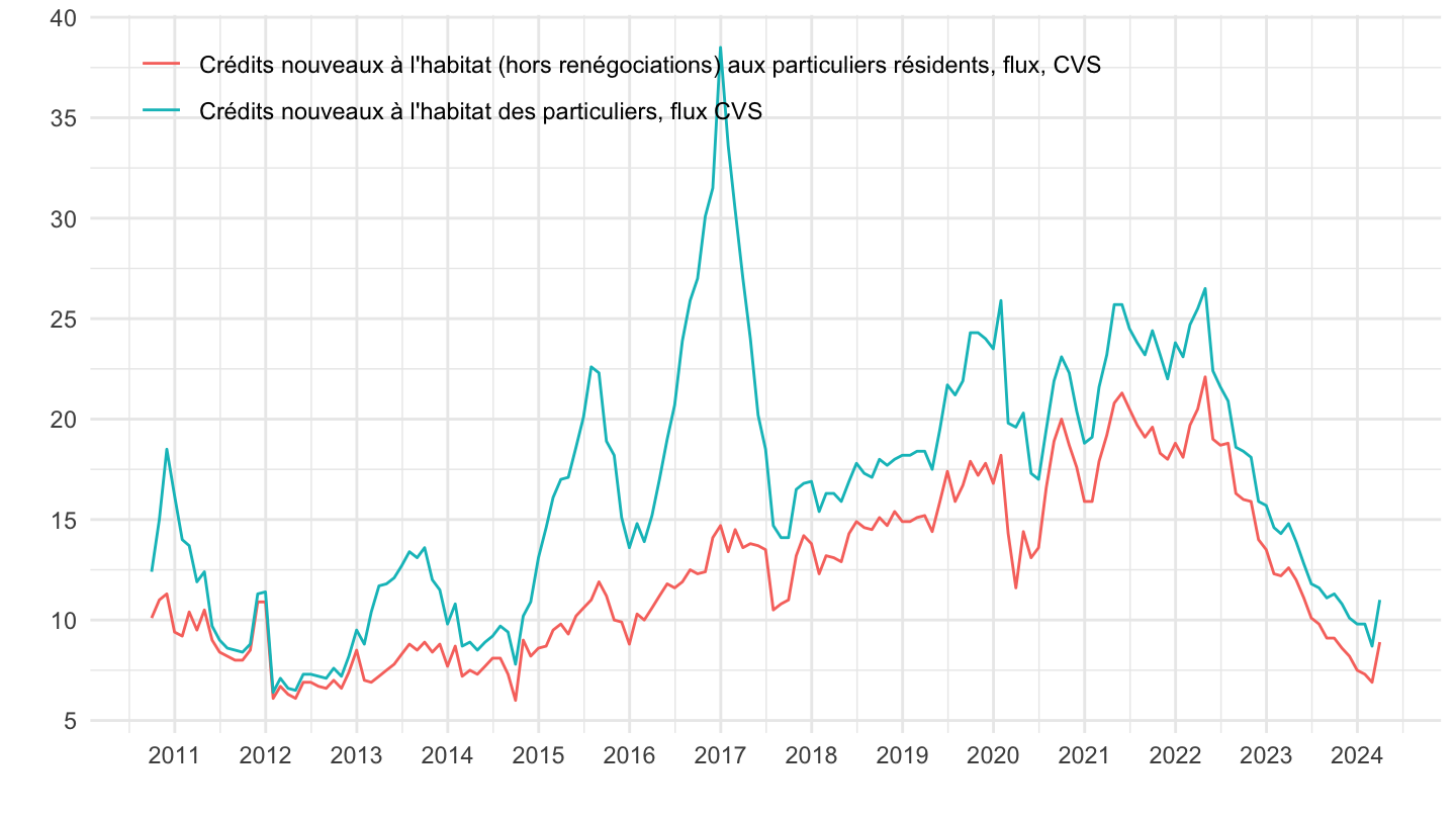

Pour en savoir plus…

LAST_COMPILE

LAST_COMPILE
2026-09-20

Last

Code

immobilier |>
  group_by(date) |>
  summarise(Nobs = n()) |>
  arrange(desc(date)) |>
  head(2) |>
  print_table_conditional()

date	Nobs
2026-07-21	1
2026-07-20	1

Related Data

Analyse des Données du Secteur Immobilier

source	dataset	Title	Updated
acpr	as160	Enquête annuelle du SGACPR sur le financement de l’habitat 2023 - as160	2026-08-01
bdf	BSI1	Agrégats monétaires - France - BSI1	2026-09-16
bdf	CPP	Prix immobilier commercial - CPP	2026-08-10
bdf	FM	Marché financier, taux - FM	2026-09-17
bdf	MIR1	Taux d’intérêt - France - MIR1	2026-09-04
bdf	RPP	Prix de l’immobilier - RPP	2026-09-17
bdf	immobilier	Immobilier en France - immobilier	2026-08-01
cgedd	nombre-vente-maison-appartement-ancien	Nombre de ventes de logements anciens cumulé sur 12 mois - nombre-vente-maison-appartement-ancien	2026-08-01
ecb	BSI	Balance Sheet Items - BSI	2026-09-17
insee	CONSTRUCTION-LOGEMENTS	Construction de logements - CONSTRUCTION-LOGEMENTS	2026-09-17
insee	ENQ-CONJ-ART-BAT	Conjoncture dans l’artisanat du bâtiment - ENQ-CONJ-ART-BAT	2026-09-17
insee	ENQ-CONJ-IND-BAT	Conjoncture dans l’industrie du bâtiment - ENQ-CONJ-IND-BAT	2026-09-17
insee	ENQ-CONJ-PROMO-IMMO	Conjoncture dans la promotion immobilière - ENQ-CONJ-PROMO-IMMO	2026-09-17
insee	ENQ-CONJ-TP	Conjoncture dans les travaux publics - ENQ-CONJ-TP	2026-09-17
insee	ILC-ILAT-ICC	Indices pour la révision d’un bail commercial ou professionnel - ILC-ILAT-ICC	2026-09-18
insee	IPLA-IPLNA-2015	Indices des prix des logements neufs et Indices Notaires-Insee des prix des logements anciens - IPLA-IPLNA-2015	2026-09-17
insee	IRL	Indice pour la révision d’un loyer d’habitation - IRL	2026-09-17
insee	PARC-LOGEMENTS	Estimations annuelles du parc de logements (EAPL) - PARC-LOGEMENTS	2026-09-04
insee	T_3217	3.217 – Principaux impôts par catégorie (En milliards d’euros) - t_3217	2026-09-18
insee	bdf2017	Budget de famille 2017 - bdf2017	2026-09-04
insee	conso-eff-fonction	Consommation effective des ménages par fonction - conso-eff-fonction	2026-08-02
notaires	arrdt	Prix au m² par arrondissement - arrdt	2026-09-17
notaires	dep	Prix au m² par département - dep	2026-09-17

Data on Log

source	dataset	Title	Updated
bdf	immobilier	Immobilier en France - immobilier	2026-08-01
bea	T10105	Table 1.1.5. Gross Domestic Product (A) (Q) - T10105	2026-07-25
ecb	EXR	Exchange Rates - EXR	2026-09-17
fred	gdp	Gross Domestic Product - gdp	2026-09-19
fred	industry	Manufacturing, Industry - industry	2026-09-19
insee	marc-salair-net-moy-sexe	Évolution du salaire annuel net moyen des salariés dans le secteur privé à temps complet selon le sexe - marc-salair-net-moy-sexe	2026-08-02
insee	reve-niv-vie-pouv-achat-trim	Évolution du revenu disponible brut et du pouvoir d’achat - Données trimestrielles - reve-niv-vie-pouv-achat-trim	2026-08-02
log	microprocessor-trend-data	Microprocessor Trend Data - microprocessor-trend-data	2026-09-18

Why Economists Should Use Log Scales More Often

source	dataset	Title	Updated
bdf	immobilier	Immobilier en France - immobilier	2026-08-01
bea	T10105	Table 1.1.5. Gross Domestic Product (A) (Q) - T10105	2026-07-25
ecb	EXR	Exchange Rates - EXR	2026-09-17
fred	gdp	Gross Domestic Product - gdp	2026-09-19
fred	industry	Manufacturing, Industry - industry	2026-09-19
insee	marc-salair-net-moy-sexe	Évolution du salaire annuel net moyen des salariés dans le secteur privé à temps complet selon le sexe - marc-salair-net-moy-sexe	2026-08-02
insee	reve-niv-vie-pouv-achat-trim	Évolution du revenu disponible brut et du pouvoir d’achat - Données trimestrielles - reve-niv-vie-pouv-achat-trim	2026-08-02
log	microprocessor-trend-data	Microprocessor Trend Data - microprocessor-trend-data	2026-09-18