| source | dataset | Title | .html | .rData |
|---|---|---|---|---|
| eurostat | sts_inppd_m | Producer prices in industry, domestic market - monthly data | 2026-07-20 | 2026-07-20 |
Producer prices in industry, domestic market - monthly data
Data - Eurostat
Info
Info
Code
include_graphics("https://ec.europa.eu/eurostat/statistics-explained/images/3/33/EU%2C_EA-19_Industrial_producer_prices%2C_total%2C_domestic_and_non-domestic_market%2C_2010_-_2022%2C_undadjusted_data_%282015_%3D_100%29_01-06-2022.png")
Data on industry
| source | dataset | Title | .html | .rData |
|---|---|---|---|---|
| eurostat | sts_inppd_m | Producer prices in industry, domestic market - monthly data | 2026-07-20 | 2026-07-20 |
| ec | INDUSTRY | Industry (sector data) | 2026-07-20 | 2026-07-20 |
| eurostat | ei_isin_m | Industry - monthly data - index (2015 = 100) (NACE Rev. 2) - ei_isin_m | 2026-07-20 | 2026-07-20 |
| eurostat | htec_trd_group4 | High-tech trade by high-tech group of products in million euro (from 2007, SITC Rev. 4) | 2026-07-20 | 2026-07-20 |
| eurostat | nama_10_a64 | National accounts aggregates by industry (up to NACE A*64) | 2026-07-17 | 2026-07-20 |
| eurostat | nama_10_a64_e | National accounts employment data by industry (up to NACE A*64) | 2026-07-20 | 2026-07-20 |
| eurostat | namq_10_a10_e | Employment A*10 industry breakdowns | 2026-07-20 | 2026-07-20 |
| eurostat | road_eqr_carmot | New registrations of passenger cars by type of motor energy and engine size - road_eqr_carmot | 2026-07-20 | 2026-07-20 |
| eurostat | sts_inpp_m | Producer prices in industry, total - monthly data | 2026-07-20 | 2026-07-20 |
| eurostat | sts_inpr_m | Production in industry - monthly data | 2026-07-20 | 2026-07-20 |
| eurostat | sts_intvnd_m | Turnover in industry, non domestic market - monthly data - sts_intvnd_m | 2026-03-24 | 2026-07-20 |
| fred | industry | Manufacturing, Industry | 2026-07-20 | 2026-07-20 |
| oecd | ALFS_EMP | Employment by activities and status (ALFS) | 2024-04-16 | 2025-05-24 |
| oecd | BERD_MA_SOF | Business enterprise R&D expenditure by main activity (focussed) and source of funds | 2024-04-16 | 2023-09-09 |
| oecd | GBARD_NABS2007 | Government budget allocations for R and D | 2024-04-16 | 2023-11-22 |
| oecd | MEI_REAL | Production and Sales (MEI) | 2024-05-12 | 2025-05-24 |
| oecd | MSTI_PUB | Main Science and Technology Indicators | 2024-09-15 | 2025-05-24 |
| oecd | SNA_TABLE4 | PPPs and exchange rates | 2024-09-15 | 2025-05-24 |
| wdi | NV.IND.EMPL.KD | Industry, value added per worker (constant 2010 USD) | 2024-01-06 | 2026-07-20 |
| wdi | NV.IND.MANF.CD | Manufacturing, value added (current USD) | 2026-07-20 | 2026-07-20 |
| wdi | NV.IND.MANF.ZS | Manufacturing, value added (% of GDP) | 2025-05-24 | 2026-07-20 |
| wdi | NV.IND.TOTL.KD | Industry (including construction), value added (constant 2015 USD) - NV.IND.TOTL.KD | 2024-01-06 | 2026-07-20 |
| wdi | NV.IND.TOTL.ZS | Industry, value added (including construction) (% of GDP) | 2025-05-24 | 2026-07-20 |
| wdi | SL.IND.EMPL.ZS | Employment in industry (% of total employment) | 2026-07-20 | 2026-07-20 |
| wdi | TX.VAL.MRCH.CD.WT | Merchandise exports (current USD) | 2024-01-06 | 2026-07-20 |
LAST_COMPILE
| LAST_COMPILE |
|---|
| 2026-07-22 |
Last
Code
sts_inppd_m %>%
  group_by(time) %>%
  summarise(Nobs = n()) %>%
  arrange(desc(time)) %>%
  head(1) %>%
print_table_conditional()| time | Nobs |
|---|---|
| 2026M03 | 1866 |
nace_r2
Code
sts_inppd_m %>%
  left_join(nace_r2, by = "nace_r2") %>%
  group_by(nace_r2, Nace_r2) %>%
  summarise(Nobs = n()) %>%
  {if (is_html_output()) datatable(., filter = 'top', rownames = F) else .}
unit
Code
sts_inppd_m %>%
  left_join(unit, by = "unit") %>%
  group_by(unit, Unit) %>%
  summarise(Nobs = n()) %>%
  arrange(-Nobs) %>%
{if (is_html_output()) print_table(.) else .}| unit | Unit | Nobs |
|---|---|---|
| PCH_PRE | Percentage change on previous period | 2045386 |
| PCH_SM | Percentage change compared to same period in previous year | 1969116 |
| I21 | Index, 2021=100 | 1686577 |
| I15 | Index, 2015=100 | 1674270 |
| I10 | Index, 2010=100 | 1095326 |
indic_bt
Code
sts_inppd_m %>%
  left_join(indic_bt, by = "indic_bt") %>%
  group_by(indic_bt, Indic_bt) %>%
  summarise(Nobs = n()) %>%
  arrange(-Nobs) %>%
{if (is_html_output()) print_table(.) else .}| indic_bt | Indic_bt | Nobs |
|---|---|---|
| PRC_PRR_DOM | Domestic producer prices | 8470675 |
geo
Code
sts_inppd_m %>%
  left_join(geo, by = "geo") %>%
  group_by(geo, Geo) %>%
  summarise(Nobs = n()) %>%
  arrange(-Nobs) %>%
  mutate(Geo = ifelse(geo == "DE", "Germany", Geo)) %>%
  mutate(Flag = gsub(" ", "-", str_to_lower(Geo)),
         Flag = paste0('<img src="../../bib/flags/vsmall/', Flag, '.png" alt="Flag">')) %>%
  select(Flag, everything()) %>%
  {if (is_html_output()) datatable(., filter = 'top', rownames = F, escape = F) else .}
time
Code
sts_inppd_m %>%
  group_by(time) %>%
  summarise(Nobs = n()) %>%
  {if (is_html_output()) datatable(., filter = 'top', rownames = F) else .}
France, Germany, Italy
All
Code
sts_inppd_m %>%
  filter(nace_r2 == "C",
         unit == "I15",
         geo %in% c("FR", "DE", "IT")) %>%
  select(geo, time, values) %>%
  group_by(geo) %>%
  mutate(values = values/values[time == "2000M01"]) %>%
  left_join(geo, by = "geo") %>%
  mutate(Geo = ifelse(geo == "DE", "Germany", Geo)) %>%
  month_to_date %>%
  ggplot() + ylab("Domestic output price index - in national currency") + xlab("") + theme_minimal() +
  geom_line(aes(x = date, y = values, color = Geo)) +
  scale_color_manual(values = c("#0055a4", "#000000", "#008c45")) +
  scale_x_date(breaks = seq(1920, 2050, 5) %>% paste0("-01-01") %>% as.Date,
               labels = date_format("%Y")) +
  add_3flags +
  theme(legend.position = "none") +
  scale_y_log10(breaks = seq(-60, 300, 10))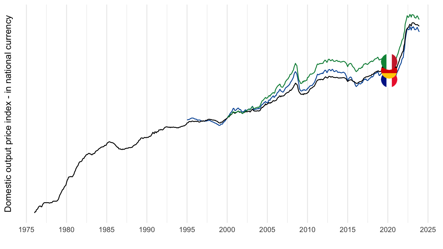
1995-
Code
sts_inppd_m %>%
  filter(nace_r2 == "C",
         unit == "I15",
         geo %in% c("FR", "DE", "IT")) %>%
  select(geo, time, values) %>%
  group_by(geo) %>%
  mutate(values = 100*values/values[time == "2000M01"]) %>%
  left_join(geo, by = "geo") %>%
  mutate(Geo = ifelse(geo == "DE", "Germany", Geo)) %>%
  month_to_date %>%
  filter(date >= as.Date("1995-01-01")) %>%
  ggplot() + ylab("Domestic output price index - in national currency") + xlab("") + theme_minimal() +
  geom_line(aes(x = date, y = values, color = Geo)) +
  scale_color_manual(values = c("#0055a4", "#000000", "#008c45")) +
  scale_x_date(breaks = seq(1920, 2050, 5) %>% paste0("-01-01") %>% as.Date,
               labels = date_format("%Y")) +
  add_3flags +
  theme(legend.position = "none") +
  scale_y_log10(breaks = seq(-60, 300, 5))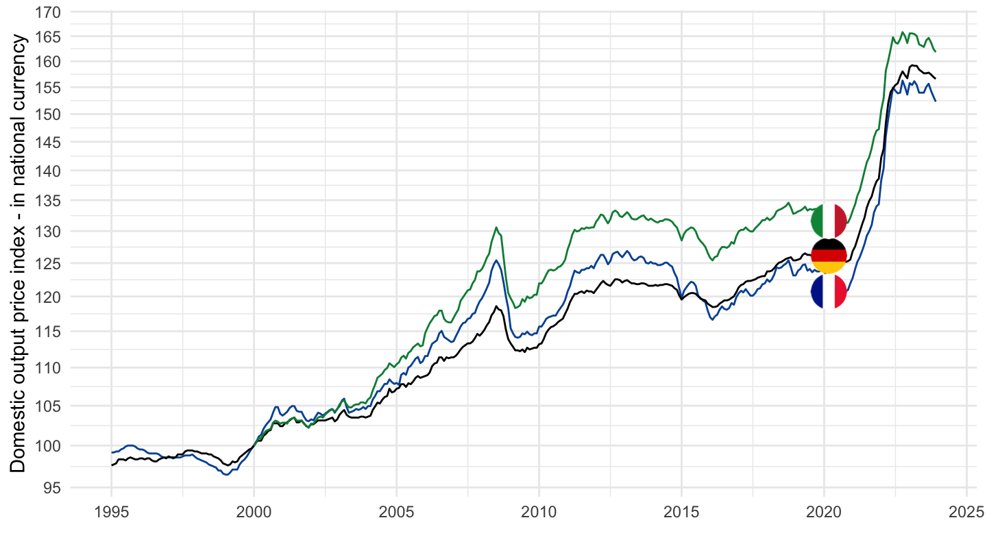
2000-
Code
sts_inppd_m %>%
  filter(nace_r2 == "C",
         unit == "I15",
         geo %in% c("FR", "DE", "IT")) %>%
  select(geo, time, values) %>%
  group_by(geo) %>%
  mutate(values = 100*values/values[time == "2000M01"]) %>%
  left_join(geo, by = "geo") %>%
  mutate(Geo = ifelse(geo == "DE", "Germany", Geo)) %>%
  month_to_date %>%
  filter(date >= as.Date("2000-01-01")) %>%
  ggplot() + ylab("Domestic output price index - in national currency") + xlab("") + theme_minimal() +
  geom_line(aes(x = date, y = values, color = Geo)) +
  scale_color_manual(values = c("#0055a4", "#000000", "#008c45")) +
  scale_x_date(breaks = seq(1920, 2050, 5) %>% paste0("-01-01") %>% as.Date,
               labels = date_format("%Y")) +
  add_3flags +
  theme(legend.position = "none") +
  scale_y_log10(breaks = seq(-60, 300, 5))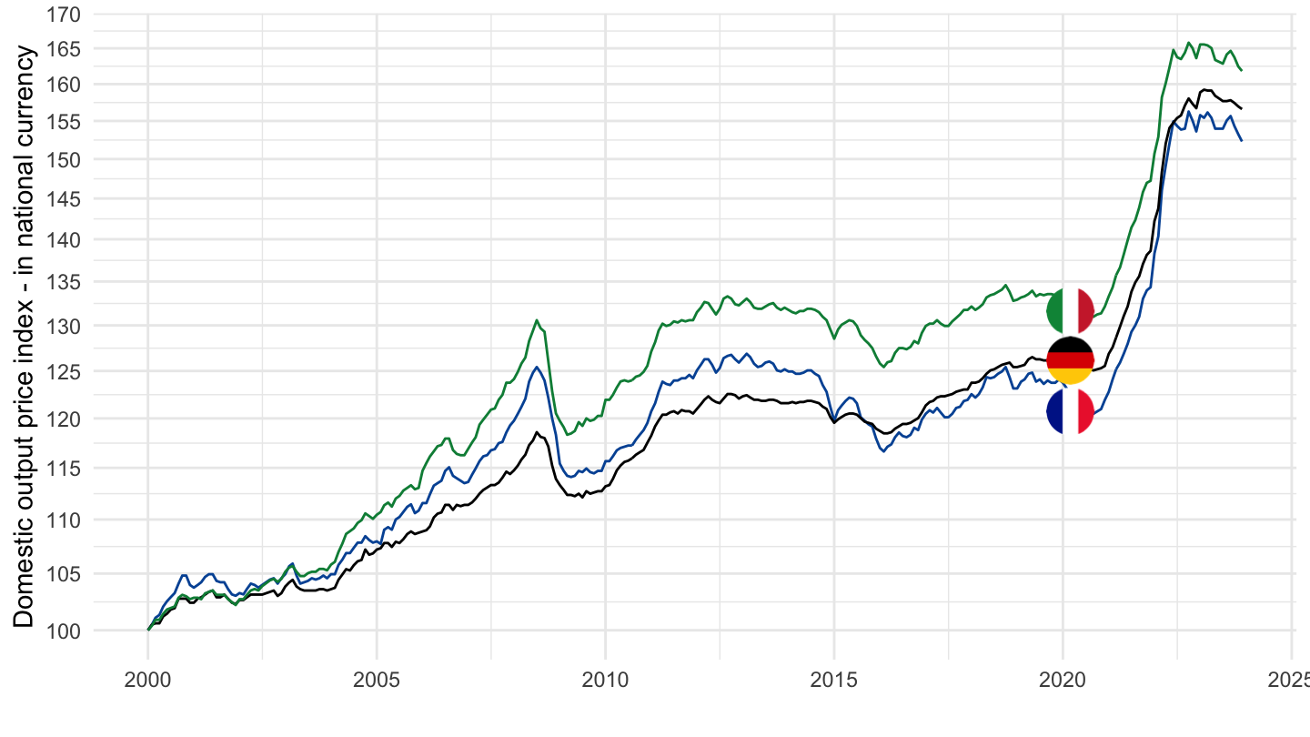
2020-
Code
sts_inppd_m %>%
  filter(nace_r2 == "C",
         unit == "I15",
         geo %in% c("FR", "DE", "IT")) %>%
  select(geo, time, values) %>%
  left_join(geo, by = "geo") %>%
  mutate(Geo = ifelse(geo == "DE", "Germany", Geo)) %>%
  month_to_date %>%
  filter(date >= as.Date("2020-01-01")) %>%
  group_by(geo) %>%
  arrange(date) %>%
  mutate(values = 100*values/values[1]) %>%
  ggplot() + ylab("Domestic output price index - in national currency") + xlab("") + theme_minimal() +
  geom_line(aes(x = date, y = values, color = Geo)) +
  scale_color_manual(values = c("#0055a4", "#000000", "#008c45")) +
  scale_x_date(breaks = "6 months",
               labels = date_format("%b %Y")) +
  add_3flags +
  theme(legend.position = "none") +
  scale_y_log10(breaks = seq(-60, 300, 5))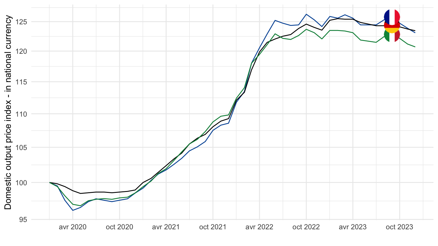
Euro Area 19
C
All
Code
sts_inpp_m %>%
  bind_rows(sts_inppd_m) %>%
  bind_rows(sts_inppnd_m) %>%
  filter(nace_r2 == "C",
         unit == "PCH_SM",
         geo %in% c("EA19")) %>%
  month_to_date %>%
  left_join(indic_bt, by = "indic_bt") %>%
  mutate(values = values/100) %>%
  ggplot(.) + geom_line(aes(x = date, y = values, color = Indic_bt)) +
  theme_minimal() + xlab("") + ylab("") +
  scale_x_date(breaks = seq(1960, 2050, 5) %>% paste0("-01-01") %>% as.Date,
               labels = date_format("%Y")) +
  scale_y_continuous(breaks = 0.01*seq(-100, 100, 5),
                     labels = percent_format(a = 1)) +
  theme(legend.position = c(0.6, 0.85),
        legend.title = element_blank())
2016-
Code
sts_inpp_m %>%
  bind_rows(sts_inppd_m) %>%
  bind_rows(sts_inppnd_m) %>%
  filter(nace_r2 == "C",
         unit == "PCH_SM",
         geo %in% c("EA19")) %>%
  month_to_date %>%
  filter(date >= as.Date("2016-01-01")) %>%
  left_join(indic_bt, by = "indic_bt") %>%
  mutate(values = values/100) %>%
  ggplot(.) + geom_line(aes(x = date, y = values, color = Indic_bt)) +
  theme_minimal() + xlab("") + ylab("") +
  scale_x_date(breaks = seq(1960, 2050, 1) %>% paste0("-01-01") %>% as.Date,
               labels = date_format("%Y")) +
  scale_y_continuous(breaks = 0.01*seq(-100, 100, 5),
                     labels = percent_format(a = 1)) +
  theme(legend.position = c(0.3, 0.85),
        legend.title = element_blank())
2020-
Code
sts_inpp_m %>%
  bind_rows(sts_inppd_m) %>%
  bind_rows(sts_inppnd_m) %>%
  filter(nace_r2 == "C",
         unit == "PCH_SM",
         geo %in% c("EA19")) %>%
  month_to_date %>%
  filter(date >= as.Date("2020-01-01")) %>%
  left_join(indic_bt, by = "indic_bt") %>%
  mutate(values = values/100) %>%
  ggplot(.) + geom_line(aes(x = date, y = values, color = Indic_bt)) +
  theme_minimal() + xlab("") + ylab("") +
  scale_x_date(breaks = seq.Date(as.Date("2019-12-01"), as.Date("2024-01-01"), "3 months"),
               labels = date_format("%b %y")) +
  scale_y_continuous(breaks = 0.01*seq(-100, 100, 5),
                     labels = percent_format(a = 1)) +
  theme(legend.position = c(0.3, 0.85),
        legend.title = element_blank())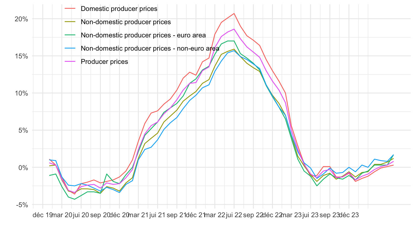
France
C
All
Code
sts_inpp_m %>%
  bind_rows(sts_inppd_m) %>%
  bind_rows(sts_inppnd_m) %>%
  filter(nace_r2 == "C",
         unit == "PCH_SM",
         geo %in% c("FR")) %>%
  month_to_date %>%
  left_join(indic_bt, by = "indic_bt") %>%
  mutate(values = values/100) %>%
  ggplot(.) + geom_line(aes(x = date, y = values, color = Indic_bt)) +
  theme_minimal() + xlab("") + ylab("") +
  scale_x_date(breaks = seq(1960, 2050, 5) %>% paste0("-01-01") %>% as.Date,
               labels = date_format("%Y")) +
  scale_y_continuous(breaks = 0.01*seq(-100, 100, 5),
                     labels = percent_format(a = 1)) +
  theme(legend.position = c(0.6, 0.85),
        legend.title = element_blank())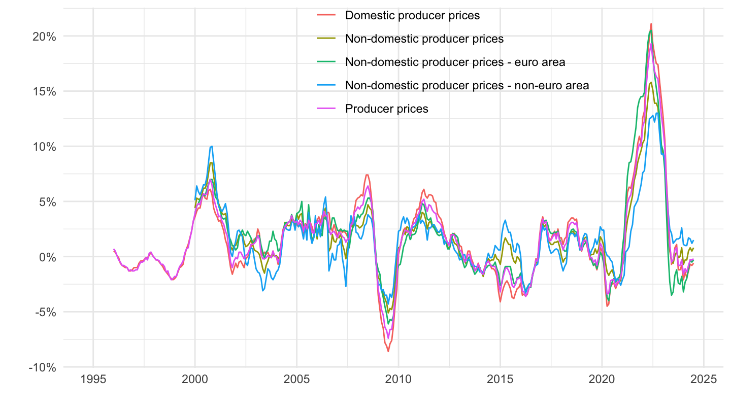
2016-
Code
sts_inpp_m %>%
  bind_rows(sts_inppd_m) %>%
  bind_rows(sts_inppnd_m) %>%
  filter(nace_r2 == "C",
         unit == "PCH_SM",
         geo %in% c("FR")) %>%
  month_to_date %>%
  filter(date >= as.Date("2016-01-01")) %>%
  left_join(indic_bt, by = "indic_bt") %>%
  mutate(values = values/100) %>%
  ggplot(.) + geom_line(aes(x = date, y = values, color = Indic_bt)) +
  theme_minimal() + xlab("") + ylab("") +
  scale_x_date(breaks = seq(1960, 2050, 1) %>% paste0("-01-01") %>% as.Date,
               labels = date_format("%Y")) +
  scale_y_continuous(breaks = 0.01*seq(-100, 100, 5),
                     labels = percent_format(a = 1)) +
  theme(legend.position = c(0.3, 0.85),
        legend.title = element_blank())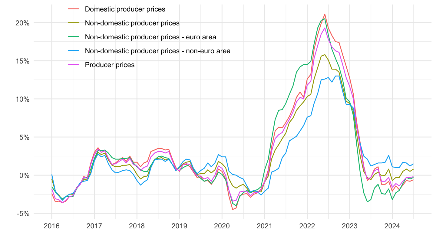
2020-
Code
sts_inpp_m %>%
  bind_rows(sts_inppd_m) %>%
  bind_rows(sts_inppnd_m) %>%
  filter(nace_r2 == "C",
         unit == "PCH_SM",
         geo %in% c("FR")) %>%
  month_to_date %>%
  filter(date >= as.Date("2020-01-01")) %>%
  left_join(indic_bt, by = "indic_bt") %>%
  mutate(values = values/100) %>%
  ggplot(.) + geom_line(aes(x = date, y = values, color = Indic_bt)) +
  theme_minimal() + xlab("") + ylab("") +
  scale_x_date(breaks = seq.Date(as.Date("2019-12-01"), as.Date("2024-01-01"), "3 months"),
               labels = date_format("%b %y")) +
  scale_y_continuous(breaks = 0.01*seq(-100, 100, 5),
                     labels = percent_format(a = 1)) +
  theme(legend.position = c(0.3, 0.85),
        legend.title = element_blank())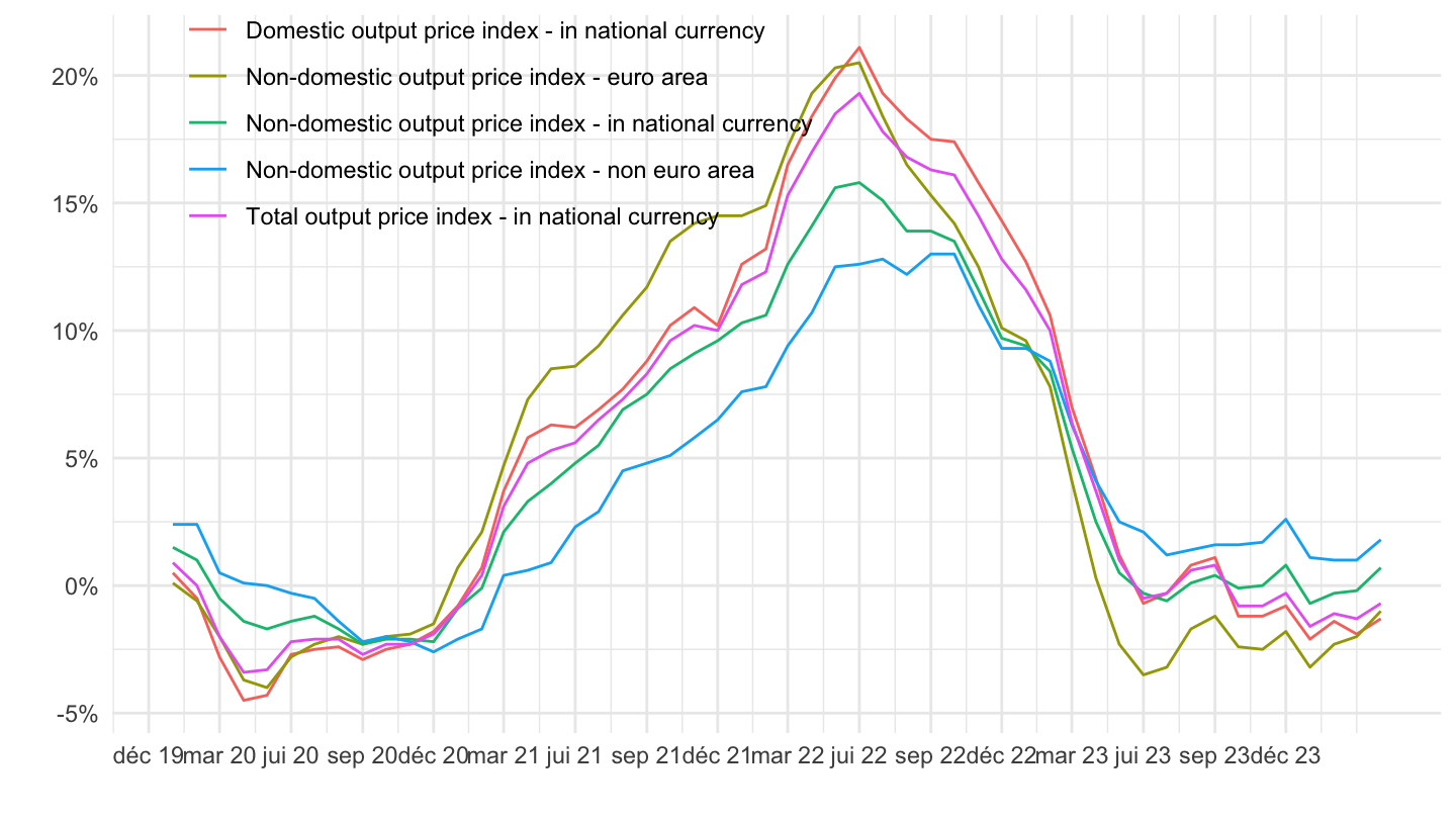
D35
All
Code
sts_inpp_m %>%
  bind_rows(sts_inppd_m) %>%
  bind_rows(sts_inppnd_m) %>%
  filter(nace_r2 == "D35",
         unit == "PCH_SM",
         geo %in% c("FR")) %>%
  month_to_date %>%
  left_join(indic_bt, by = "indic_bt") %>%
  mutate(values = values/100) %>%
  ggplot(.) + geom_line(aes(x = date, y = values, color = Indic_bt)) +
  theme_minimal() + xlab("") + ylab("") +
  scale_x_date(breaks = seq(1960, 2050, 5) %>% paste0("-01-01") %>% as.Date,
               labels = date_format("%Y")) +
  scale_y_continuous(breaks = 0.01*seq(-100, 1000, 20),
                     labels = percent_format(a = 1)) +
  theme(legend.position = c(0.6, 0.85),
        legend.title = element_blank())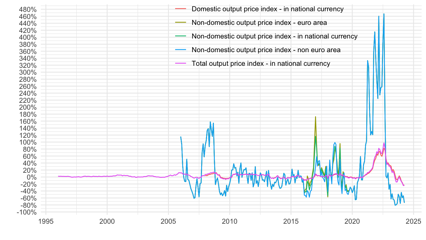
2016-
Code
sts_inpp_m %>%
  bind_rows(sts_inppd_m) %>%
  bind_rows(sts_inppnd_m) %>%
  filter(nace_r2 == "D35",
         unit == "PCH_SM",
         geo %in% c("FR")) %>%
  month_to_date %>%
  filter(date >= as.Date("2016-01-01")) %>%
  left_join(indic_bt, by = "indic_bt") %>%
  mutate(values = values/100) %>%
  ggplot(.) + geom_line(aes(x = date, y = values, color = Indic_bt)) +
  theme_minimal() + xlab("") + ylab("") +
  scale_x_date(breaks = seq(1960, 2050, 1) %>% paste0("-01-01") %>% as.Date,
               labels = date_format("%Y")) +
  scale_y_continuous(breaks = 0.01*seq(-100, 1000, 20),
                     labels = percent_format(a = 1)) +
  theme(legend.position = c(0.3, 0.85),
        legend.title = element_blank())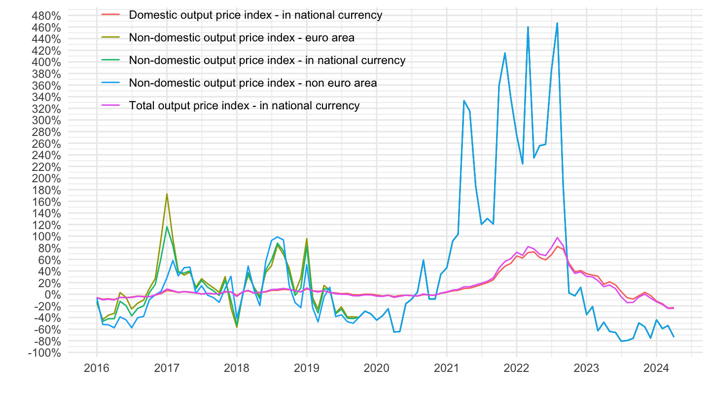
2020-
Code
sts_inpp_m %>%
  bind_rows(sts_inppd_m) %>%
  bind_rows(sts_inppnd_m) %>%
  filter(nace_r2 == "D35",
         unit == "PCH_SM",
         geo %in% c("FR")) %>%
  month_to_date %>%
  filter(date >= as.Date("2020-01-01")) %>%
  left_join(indic_bt, by = "indic_bt") %>%
  mutate(values = values/100) %>%
  ggplot(.) + geom_line(aes(x = date, y = values, color = Indic_bt)) +
  theme_minimal() + xlab("") + ylab("") +
  scale_x_date(breaks = seq.Date(as.Date("2019-12-01"), as.Date("2024-01-01"), "3 months"),
               labels = date_format("%b %y")) +
  scale_y_continuous(breaks = 0.01*seq(-100, 1000, 20),
                     labels = percent_format(a = 1)) +
  theme(legend.position = c(0.3, 0.85),
        legend.title = element_blank())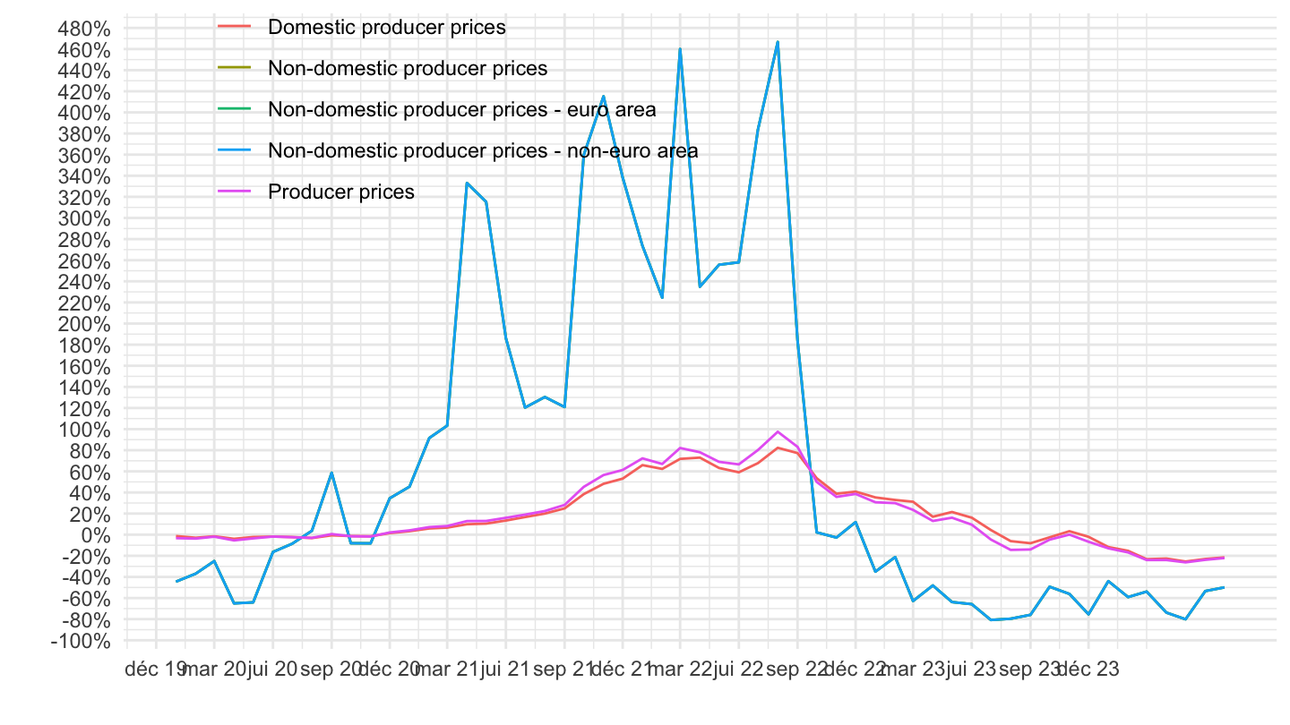
MIG_NRG - Energy
All
Code
sts_inpp_m %>%
  bind_rows(sts_inppd_m) %>%
  bind_rows(sts_inppnd_m) %>%
  filter(nace_r2 == "MIG_NRG",
         unit == "PCH_SM",
         geo %in% c("FR")) %>%
  month_to_date %>%
  left_join(indic_bt, by = "indic_bt") %>%
  mutate(values = values/100) %>%
  ggplot(.) + geom_line(aes(x = date, y = values, color = Indic_bt)) +
  theme_minimal() + xlab("") + ylab("") +
  scale_x_date(breaks = seq(1960, 2050, 5) %>% paste0("-01-01") %>% as.Date,
               labels = date_format("%Y")) +
  scale_y_continuous(breaks = 0.01*seq(-100, 300, 20),
                     labels = percent_format(a = 1)) +
  theme(legend.position = c(0.6, 0.85),
        legend.title = element_blank())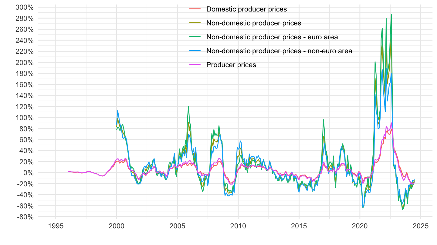
2016-
Code
sts_inpp_m %>%
  bind_rows(sts_inppd_m) %>%
  bind_rows(sts_inppnd_m) %>%
  filter(nace_r2 == "MIG_NRG",
         unit == "PCH_SM",
         geo %in% c("FR")) %>%
  month_to_date %>%
  filter(date >= as.Date("2016-01-01")) %>%
  left_join(indic_bt, by = "indic_bt") %>%
  mutate(values = values/100) %>%
  ggplot(.) + geom_line(aes(x = date, y = values, color = Indic_bt)) +
  theme_minimal() + xlab("") + ylab("") +
  scale_x_date(breaks = seq(1960, 2050, 1) %>% paste0("-01-01") %>% as.Date,
               labels = date_format("%Y")) +
  scale_y_continuous(breaks = 0.01*seq(-100, 300, 20),
                     labels = percent_format(a = 1)) +
  theme(legend.position = c(0.3, 0.85),
        legend.title = element_blank())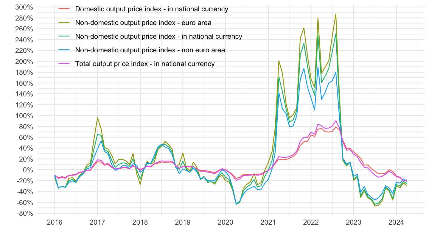
2020-
Code
sts_inpp_m %>%
  bind_rows(sts_inppd_m) %>%
  bind_rows(sts_inppnd_m) %>%
  filter(nace_r2 == "MIG_NRG",
         unit == "PCH_SM",
         geo %in% c("FR")) %>%
  month_to_date %>%
  filter(date >= as.Date("2020-01-01")) %>%
  left_join(indic_bt, by = "indic_bt") %>%
  mutate(values = values/100) %>%
  ggplot(.) + geom_line(aes(x = date, y = values, color = Indic_bt)) +
  theme_minimal() + xlab("") + ylab("") +
  scale_x_date(breaks = seq.Date(as.Date("2019-12-01"), as.Date("2024-01-01"), "3 months"),
               labels = date_format("%b %y")) +
  scale_y_continuous(breaks = 0.01*seq(-100, 300, 20),
                     labels = percent_format(a = 1)) +
  theme(legend.position = c(0.3, 0.85),
        legend.title = element_blank())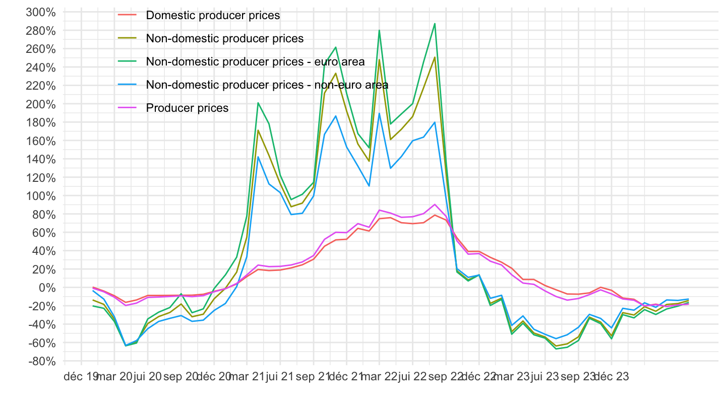
MIG_COG - Consumer Goods
All
Code
sts_inpp_m %>%
  bind_rows(sts_inppd_m) %>%
  bind_rows(sts_inppnd_m) %>%
  filter(nace_r2 == "MIG_COG",
         unit == "PCH_SM",
         geo %in% c("FR")) %>%
  month_to_date %>%
  left_join(indic_bt, by = "indic_bt") %>%
  mutate(values = values/100) %>%
  ggplot(.) + geom_line(aes(x = date, y = values, color = Indic_bt)) +
  theme_minimal() + xlab("") + ylab("") +
  scale_x_date(breaks = seq(1960, 2050, 5) %>% paste0("-01-01") %>% as.Date,
               labels = date_format("%Y")) +
  scale_y_continuous(breaks = 0.01*seq(-100, 300, 2),
                     labels = percent_format(a = 1)) +
  theme(legend.position = c(0.6, 0.85),
        legend.title = element_blank())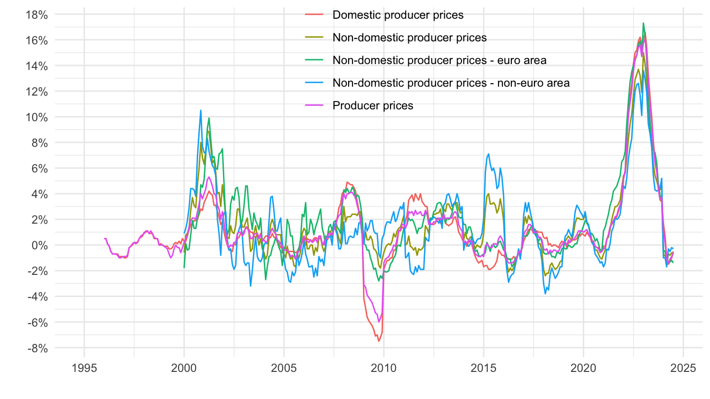
2016-
Code
sts_inpp_m %>%
  bind_rows(sts_inppd_m) %>%
  bind_rows(sts_inppnd_m) %>%
  filter(nace_r2 == "MIG_COG",
         unit == "PCH_SM",
         geo %in% c("FR")) %>%
  month_to_date %>%
  filter(date >= as.Date("2016-01-01")) %>%
  left_join(indic_bt, by = "indic_bt") %>%
  mutate(values = values/100) %>%
  ggplot(.) + geom_line(aes(x = date, y = values, color = Indic_bt)) +
  theme_minimal() + xlab("") + ylab("") +
  scale_x_date(breaks = seq(1960, 2050, 1) %>% paste0("-01-01") %>% as.Date,
               labels = date_format("%Y")) +
  scale_y_continuous(breaks = 0.01*seq(-100, 300, 2),
                     labels = percent_format(a = 1)) +
  theme(legend.position = c(0.3, 0.85),
        legend.title = element_blank())
2020-
Code
sts_inpp_m %>%
  bind_rows(sts_inppd_m) %>%
  bind_rows(sts_inppnd_m) %>%
  filter(nace_r2 == "MIG_COG",
         unit == "PCH_SM",
         geo %in% c("FR")) %>%
  month_to_date %>%
  filter(date >= as.Date("2020-01-01")) %>%
  left_join(indic_bt, by = "indic_bt") %>%
  mutate(values = values/100) %>%
  ggplot(.) + geom_line(aes(x = date, y = values, color = Indic_bt)) +
  theme_minimal() + xlab("") + ylab("") +
  scale_x_date(breaks = seq.Date(as.Date("2019-12-01"), as.Date("2024-01-01"), "3 months"),
               labels = date_format("%b %y")) +
  scale_y_continuous(breaks = 0.01*seq(-100, 300, 2),
                     labels = percent_format(a = 1)) +
  theme(legend.position = c(0.3, 0.85),
        legend.title = element_blank())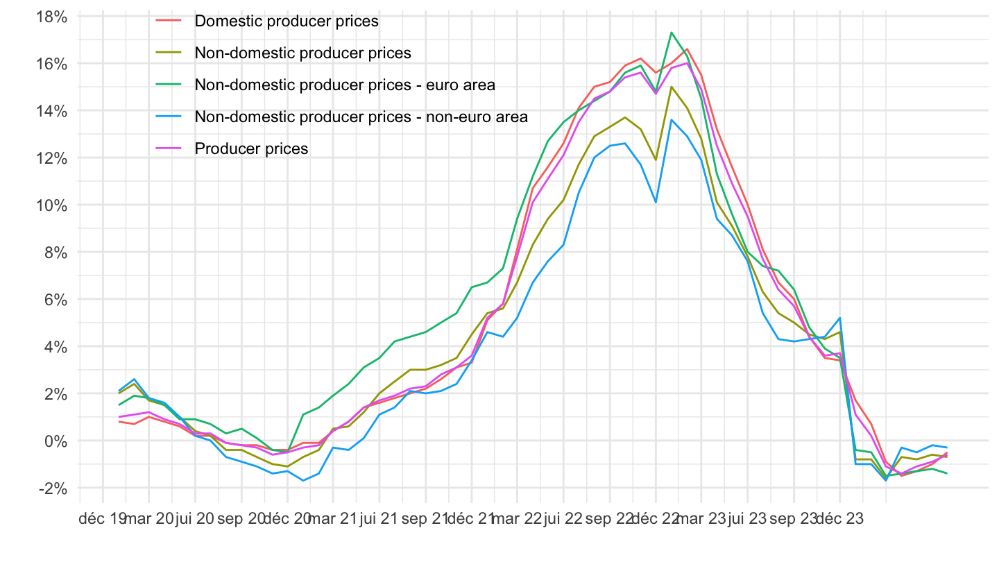
MIG_CAG - Capital Goods
All
Code
sts_inpp_m %>%
  bind_rows(sts_inppd_m) %>%
  bind_rows(sts_inppnd_m) %>%
  filter(nace_r2 == "MIG_CAG",
         unit == "PCH_SM",
         geo %in% c("FR")) %>%
  month_to_date %>%
  left_join(indic_bt, by = "indic_bt") %>%
  mutate(values = values/100) %>%
  ggplot(.) + geom_line(aes(x = date, y = values, color = Indic_bt)) +
  theme_minimal() + xlab("") + ylab("") +
  scale_x_date(breaks = seq(1960, 2050, 5) %>% paste0("-01-01") %>% as.Date,
               labels = date_format("%Y")) +
  scale_y_continuous(breaks = 0.01*seq(-100, 300, 2),
                     labels = percent_format(a = 1)) +
  theme(legend.position = c(0.6, 0.85),
        legend.title = element_blank())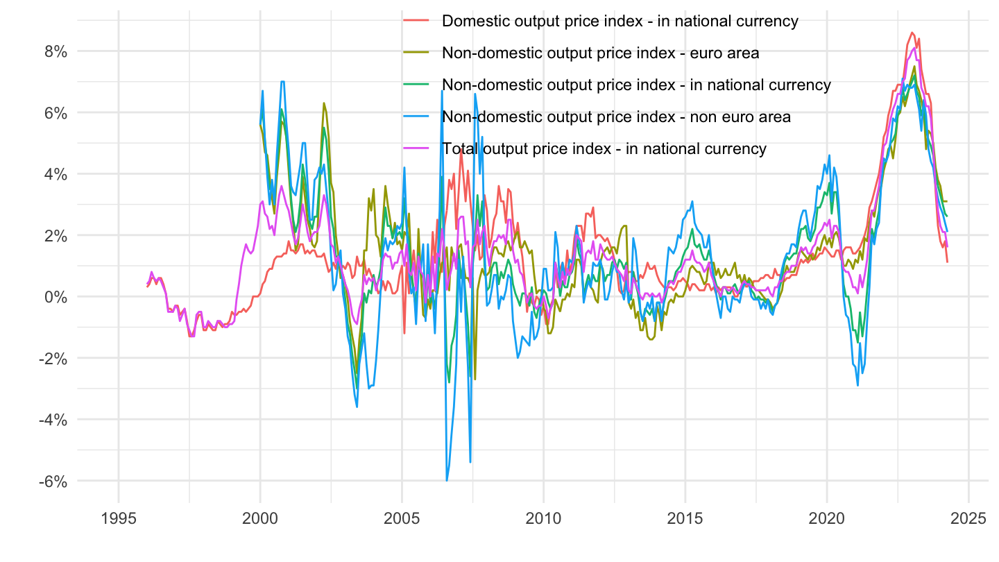
2016-
Code
sts_inpp_m %>%
  bind_rows(sts_inppd_m) %>%
  bind_rows(sts_inppnd_m) %>%
  filter(nace_r2 == "MIG_CAG",
         unit == "PCH_SM",
         geo %in% c("FR")) %>%
  month_to_date %>%
  filter(date >= as.Date("2016-01-01")) %>%
  left_join(indic_bt, by = "indic_bt") %>%
  mutate(values = values/100) %>%
  ggplot(.) + geom_line(aes(x = date, y = values, color = Indic_bt)) +
  theme_minimal() + xlab("") + ylab("") +
  scale_x_date(breaks = seq(1960, 2050, 1) %>% paste0("-01-01") %>% as.Date,
               labels = date_format("%Y")) +
  scale_y_continuous(breaks = 0.01*seq(-100, 300, 2),
                     labels = percent_format(a = 1)) +
  theme(legend.position = c(0.3, 0.85),
        legend.title = element_blank())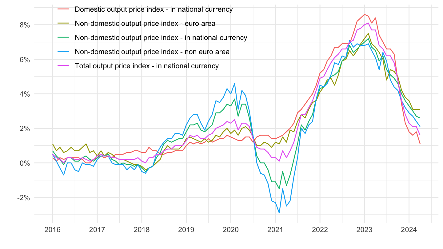
2020-
Code
sts_inpp_m %>%
  bind_rows(sts_inppd_m) %>%
  bind_rows(sts_inppnd_m) %>%
  filter(nace_r2 == "MIG_CAG",
         unit == "PCH_SM",
         geo %in% c("FR")) %>%
  month_to_date %>%
  filter(date >= as.Date("2020-01-01")) %>%
  left_join(indic_bt, by = "indic_bt") %>%
  mutate(values = values/100) %>%
  ggplot(.) + geom_line(aes(x = date, y = values, color = Indic_bt)) +
  theme_minimal() + xlab("") + ylab("") +
  scale_x_date(breaks = seq.Date(as.Date("2019-12-01"), as.Date("2024-01-01"), "3 months"),
               labels = date_format("%b %y")) +
  scale_y_continuous(breaks = 0.01*seq(-100, 300, 2),
                     labels = percent_format(a = 1)) +
  theme(legend.position = c(0.3, 0.85),
        legend.title = element_blank())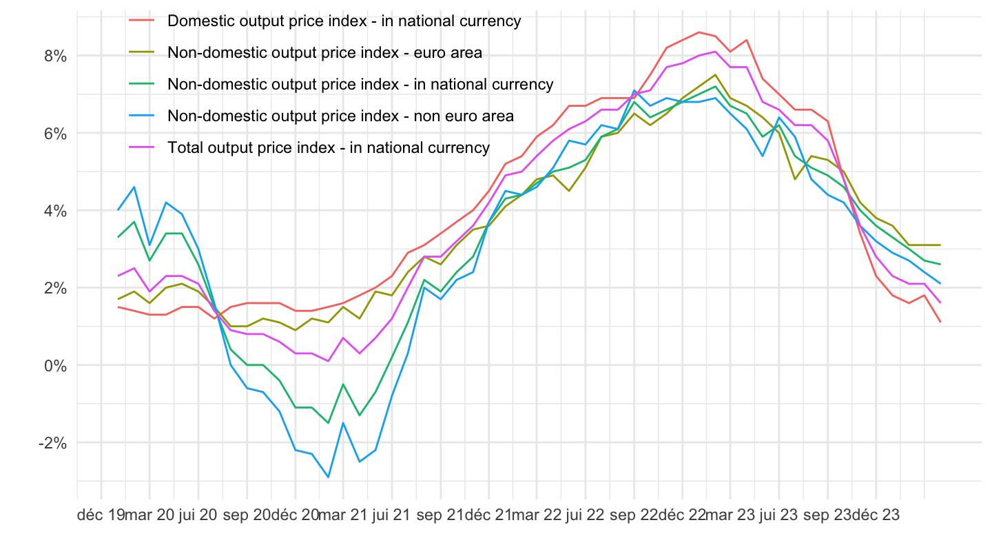
MIG_ING - Intermediate goods
All
Code
sts_inpp_m %>%
  bind_rows(sts_inppd_m) %>%
  bind_rows(sts_inppnd_m) %>%
  filter(nace_r2 == "MIG_ING",
         unit == "PCH_SM",
         geo %in% c("FR")) %>%
  month_to_date %>%
  left_join(indic_bt, by = "indic_bt") %>%
  mutate(values = values/100) %>%
  ggplot(.) + geom_line(aes(x = date, y = values, color = Indic_bt)) +
  theme_minimal() + xlab("") + ylab("") +
  scale_x_date(breaks = seq(1960, 2050, 5) %>% paste0("-01-01") %>% as.Date,
               labels = date_format("%Y")) +
  scale_y_continuous(breaks = 0.01*seq(-100, 300, 2),
                     labels = percent_format(a = 1)) +
  theme(legend.position = c(0.6, 0.85),
        legend.title = element_blank())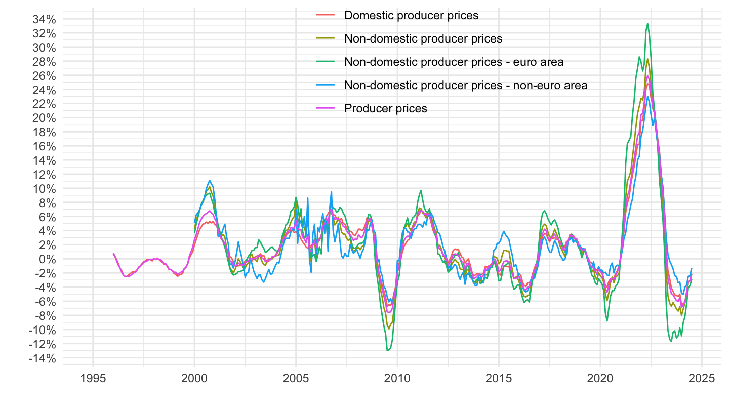
2016-
Code
sts_inpp_m %>%
  bind_rows(sts_inppd_m) %>%
  bind_rows(sts_inppnd_m) %>%
  filter(nace_r2 == "MIG_ING",
         unit == "PCH_SM",
         geo %in% c("FR")) %>%
  month_to_date %>%
  filter(date >= as.Date("2016-01-01")) %>%
  left_join(indic_bt, by = "indic_bt") %>%
  mutate(values = values/100) %>%
  ggplot(.) + geom_line(aes(x = date, y = values, color = Indic_bt)) +
  theme_minimal() + xlab("") + ylab("") +
  scale_x_date(breaks = seq(1960, 2050, 1) %>% paste0("-01-01") %>% as.Date,
               labels = date_format("%Y")) +
  scale_y_continuous(breaks = 0.01*seq(-100, 300, 2),
                     labels = percent_format(a = 1)) +
  theme(legend.position = c(0.3, 0.85),
        legend.title = element_blank())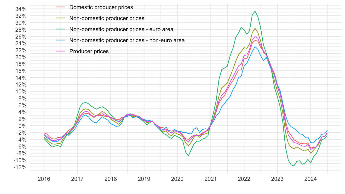
2020-
Code
sts_inpp_m %>%
  bind_rows(sts_inppd_m) %>%
  bind_rows(sts_inppnd_m) %>%
  filter(nace_r2 == "MIG_ING",
         unit == "PCH_SM",
         geo %in% c("FR")) %>%
  month_to_date %>%
  filter(date >= as.Date("2020-01-01")) %>%
  left_join(indic_bt, by = "indic_bt") %>%
  mutate(values = values/100) %>%
  ggplot(.) + geom_line(aes(x = date, y = values, color = Indic_bt)) +
  theme_minimal() + xlab("") + ylab("") +
  scale_x_date(breaks = seq.Date(as.Date("2019-12-01"), as.Date("2024-01-01"), "3 months"),
               labels = date_format("%b %y")) +
  scale_y_continuous(breaks = 0.01*seq(-100, 300, 2),
                     labels = percent_format(a = 1)) +
  theme(legend.position = c(0.3, 0.85),
        legend.title = element_blank())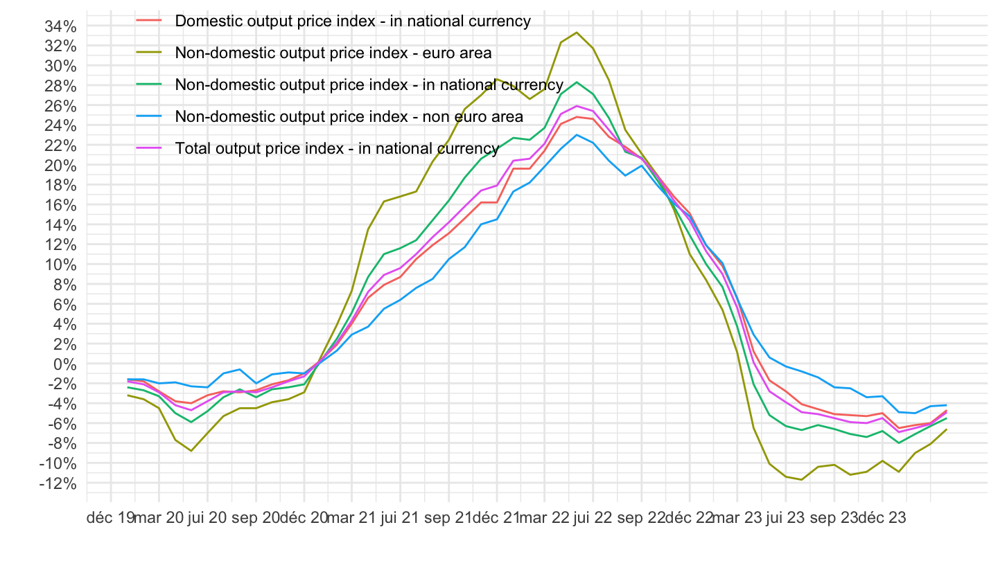
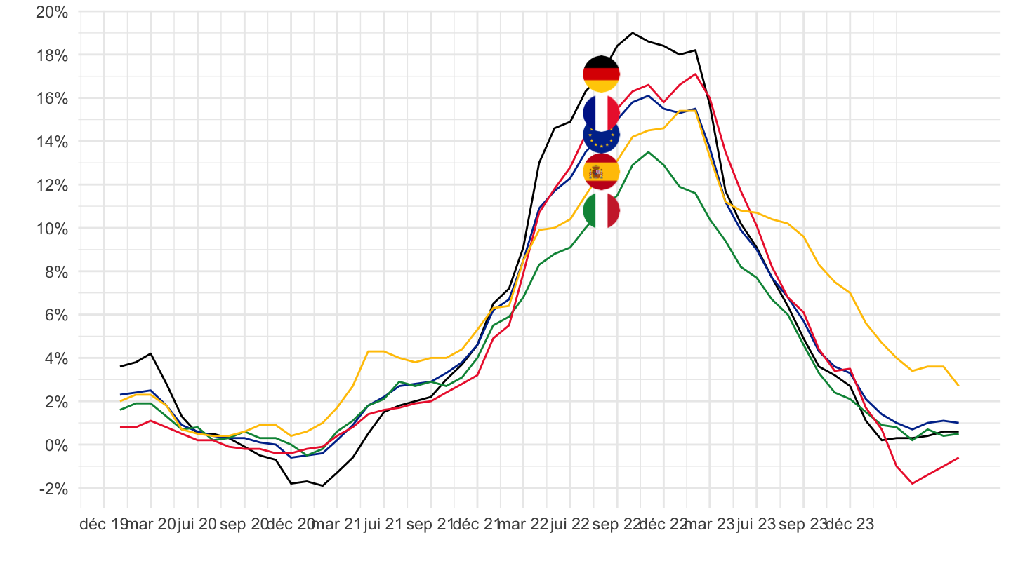
France, Germany, Italy, Spain, Europe
C
All
Code
sts_inppd_m %>%
  filter(nace_r2 == "C",
         unit == "PCH_SM",
         geo %in% c("FR", "DE", "ES", "IT", "EA19")) %>%
  month_to_date %>%
  left_join(geo, by = "geo") %>%
  mutate(Geo = ifelse(geo == "EA19", "Europe", Geo)) %>%
  left_join(colors, by = c("Geo" = "country")) %>%
  mutate(values = values/100) %>%
  ggplot(.) + geom_line(aes(x = date, y = values, color = color)) +
  theme_minimal() + xlab("") + ylab("") +
  scale_x_date(breaks = seq(1960, 2050, 5) %>% paste0("-01-01") %>% as.Date,
               labels = date_format("%Y")) +
  scale_y_continuous(breaks = 0.01*seq(-100, 100, 5),
                     labels = percent_format(a = 1)) +
  scale_color_identity() + add_5flags +
  theme(legend.position = c(0.75, 0.90),
        legend.title = element_blank())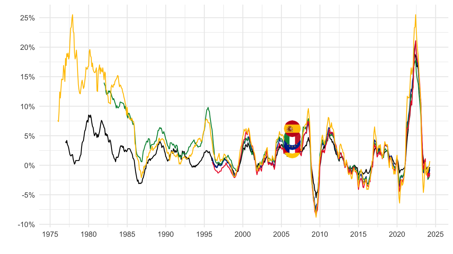
1995-
Code
sts_inppd_m %>%
  filter(nace_r2 == "C",
         unit == "PCH_SM",
         geo %in% c("FR", "DE", "ES", "IT", "EA19")) %>%
  month_to_date %>%
  filter(date >= as.Date("1995-01-01")) %>%
  left_join(geo, by = "geo") %>%
  mutate(Geo = ifelse(geo == "EA19", "Europe", Geo)) %>%
  left_join(colors, by = c("Geo" = "country")) %>%
  mutate(values = values/100) %>%
  ggplot(.) + geom_line(aes(x = date, y = values, color = color)) +
  theme_minimal() + xlab("") + ylab("") +
  scale_x_date(breaks = seq(1960, 2050, 5) %>% paste0("-01-01") %>% as.Date,
               labels = date_format("%Y")) +
  scale_y_continuous(breaks = 0.01*seq(-20, 100, 5),
                     labels = percent_format(a = 1)) +
  scale_color_identity() + add_5flags +
  theme(legend.position = c(0.75, 0.90),
        legend.title = element_blank())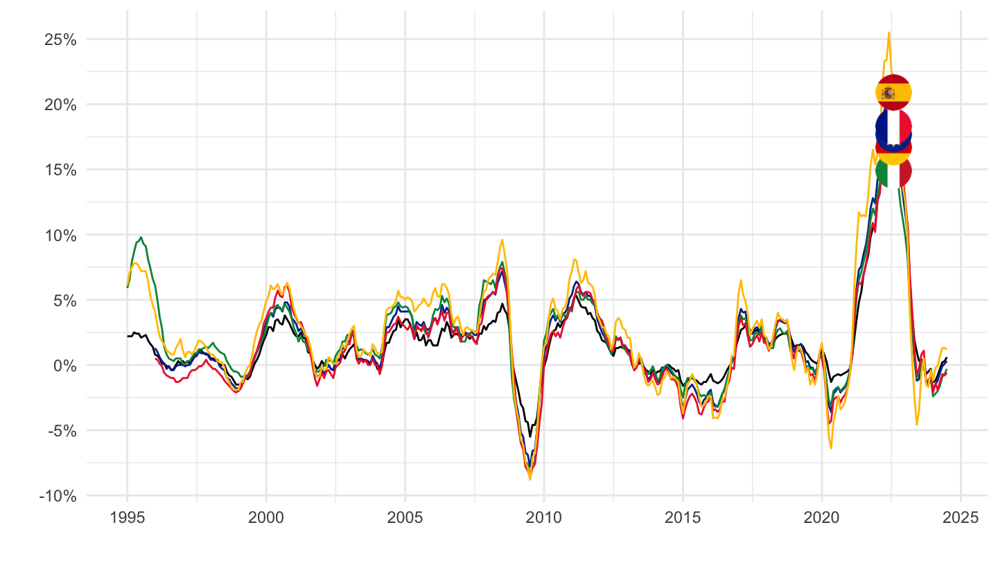
2016-
Code
sts_inppd_m %>%
  filter(nace_r2 == "C",
         unit == "PCH_SM",
         geo %in% c("FR", "DE", "ES", "IT", "EA19")) %>%
  month_to_date %>%
  filter(date >= as.Date("2016-01-01")) %>%
  left_join(geo, by = "geo") %>%
  mutate(Geo = ifelse(geo == "EA19", "Europe", Geo)) %>%
  left_join(colors, by = c("Geo" = "country")) %>%
  mutate(values = values/100) %>%
  ggplot(.) + geom_line(aes(x = date, y = values, color = color)) +
  theme_minimal() + xlab("") + ylab("") +
  scale_x_date(breaks = seq(1960, 2050, 1) %>% paste0("-01-01") %>% as.Date,
               labels = date_format("%Y")) +
  scale_y_continuous(breaks = 0.01*seq(-20, 100, 5),
                     labels = percent_format(a = 1)) +
  scale_color_identity() + add_5flags +
  theme(legend.position = c(0.75, 0.90),
        legend.title = element_blank())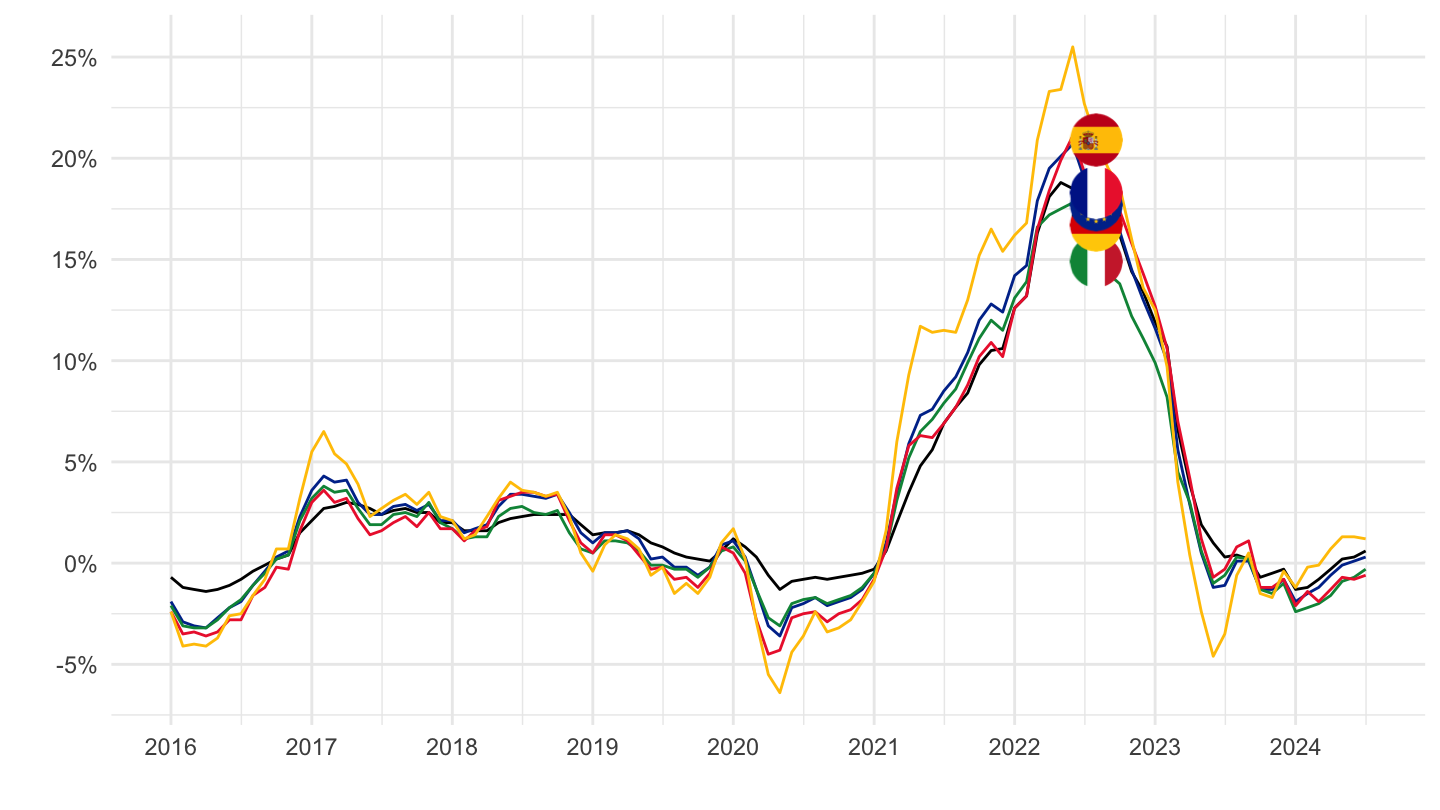
2020-
Code
sts_inppd_m %>%
  filter(nace_r2 == "C",
         unit == "PCH_SM",
         geo %in% c("FR", "DE", "ES", "IT", "EA19")) %>%
  month_to_date %>%
  filter(date >= as.Date("2020-01-01")) %>%
  left_join(geo, by = "geo") %>%
  mutate(Geo = ifelse(geo == "EA19", "Europe", Geo)) %>%
  left_join(colors, by = c("Geo" = "country")) %>%
  mutate(values = values/100) %>%
  ggplot(.) + geom_line(aes(x = date, y = values, color = color)) +
  theme_minimal() + xlab("") + ylab("") +
  scale_x_date(breaks = seq.Date(as.Date("2019-12-01"), as.Date("2024-01-01"), "3 months"),
               labels = date_format("%b %y")) +
  scale_y_continuous(breaks = 0.01*seq(-20, 100, 2),
                     labels = percent_format(a = 1)) +
  scale_color_identity() + add_5flags +
  theme(legend.position = c(0.75, 0.90),
        legend.title = element_blank())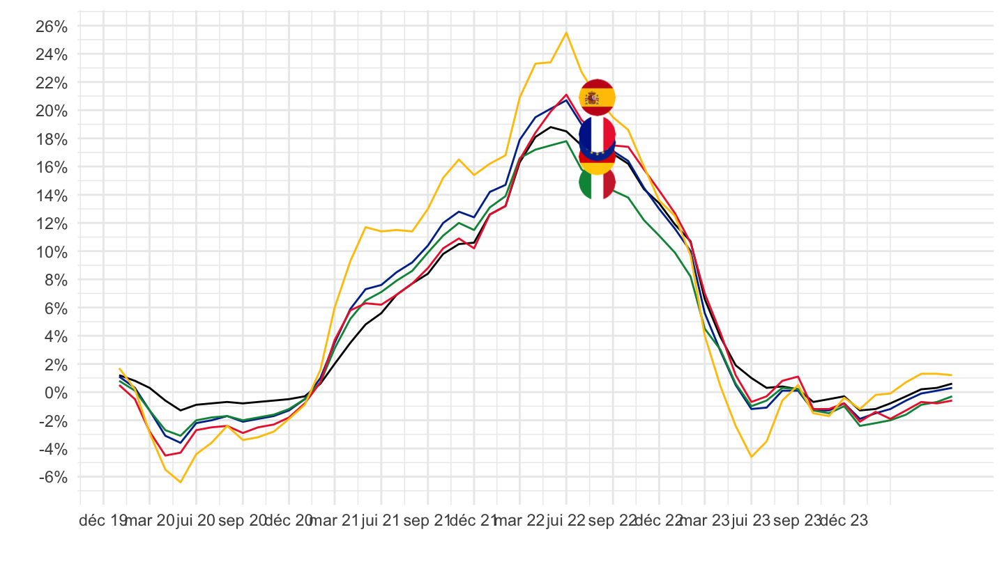
D35 - Electricity, gas, steam and air conditioning supply
All
Code
sts_inppd_m %>%
  filter(nace_r2 == "D35",
         unit == "PCH_SM",
         geo %in% c("FR", "DE", "ES", "IT", "EA19")) %>%
  month_to_date %>%
  left_join(geo, by = "geo") %>%
  mutate(Geo = ifelse(geo == "EA19", "Europe", Geo)) %>%
  left_join(colors, by = c("Geo" = "country")) %>%
  mutate(values = values/100) %>%
  ggplot(.) + geom_line(aes(x = date, y = values, color = color)) +
  theme_minimal() + xlab("") + ylab("") +
  scale_x_date(breaks = seq(1960, 2050, 5) %>% paste0("-01-01") %>% as.Date,
               labels = date_format("%Y")) +
  scale_y_continuous(breaks = 0.01*seq(-100, 200, 20),
                     labels = percent_format(a = 1)) +
  scale_color_identity() + add_5flags +
  theme(legend.position = c(0.75, 0.90),
        legend.title = element_blank())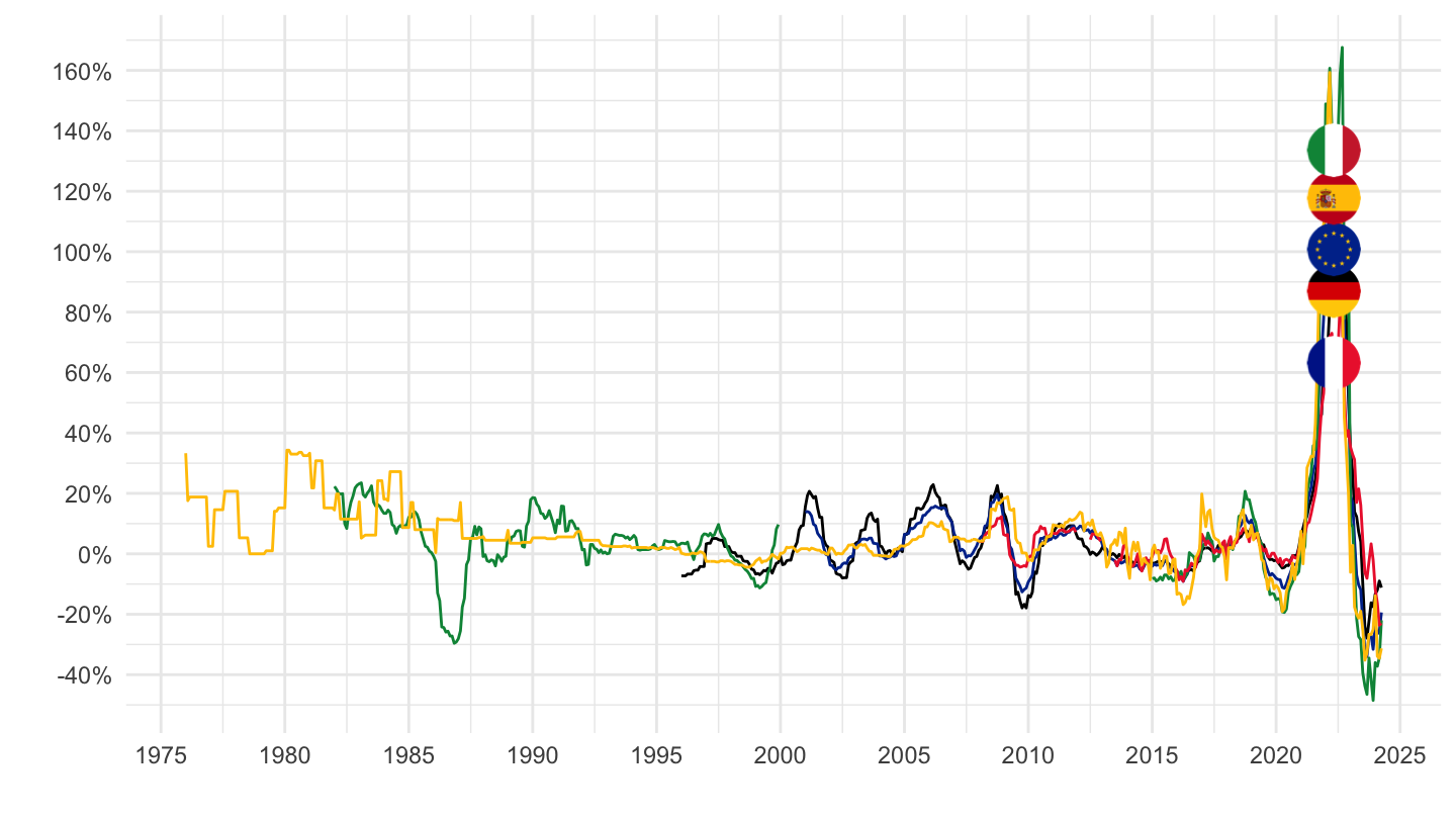
1995-
Code
sts_inppd_m %>%
  filter(nace_r2 == "D35",
         unit == "PCH_SM",
         geo %in% c("FR", "DE", "ES", "IT", "EA19")) %>%
  month_to_date %>%
  filter(date >= as.Date("1995-01-01")) %>%
  left_join(geo, by = "geo") %>%
  mutate(Geo = ifelse(geo == "EA19", "Europe", Geo)) %>%
  left_join(colors, by = c("Geo" = "country")) %>%
  mutate(values = values/100) %>%
  ggplot(.) + geom_line(aes(x = date, y = values, color = color)) +
  theme_minimal() + xlab("") + ylab("") +
  scale_x_date(breaks = seq(1960, 2050, 5) %>% paste0("-01-01") %>% as.Date,
               labels = date_format("%Y")) +
  scale_y_continuous(breaks = 0.01*seq(-100, 200, 20),
                     labels = percent_format(a = 1)) +
  scale_color_identity() + add_5flags +
  theme(legend.position = c(0.75, 0.90),
        legend.title = element_blank())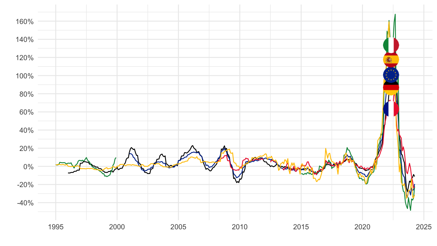
2016-
Code
sts_inppd_m %>%
  filter(nace_r2 == "D35",
         unit == "PCH_SM",
         geo %in% c("FR", "DE", "ES", "IT", "EA19")) %>%
  month_to_date %>%
  filter(date >= as.Date("2016-01-01")) %>%
  left_join(geo, by = "geo") %>%
  mutate(Geo = ifelse(geo == "EA19", "Europe", Geo)) %>%
  left_join(colors, by = c("Geo" = "country")) %>%
  mutate(values = values/100) %>%
  ggplot(.) + geom_line(aes(x = date, y = values, color = color)) +
  theme_minimal() + xlab("") + ylab("") +
  scale_x_date(breaks = seq(1960, 2050, 1) %>% paste0("-01-01") %>% as.Date,
               labels = date_format("%Y")) +
  scale_y_continuous(breaks = 0.01*seq(-100, 200, 20),
                     labels = percent_format(a = 1)) +
  scale_color_identity() + add_5flags +
  theme(legend.position = c(0.75, 0.90),
        legend.title = element_blank())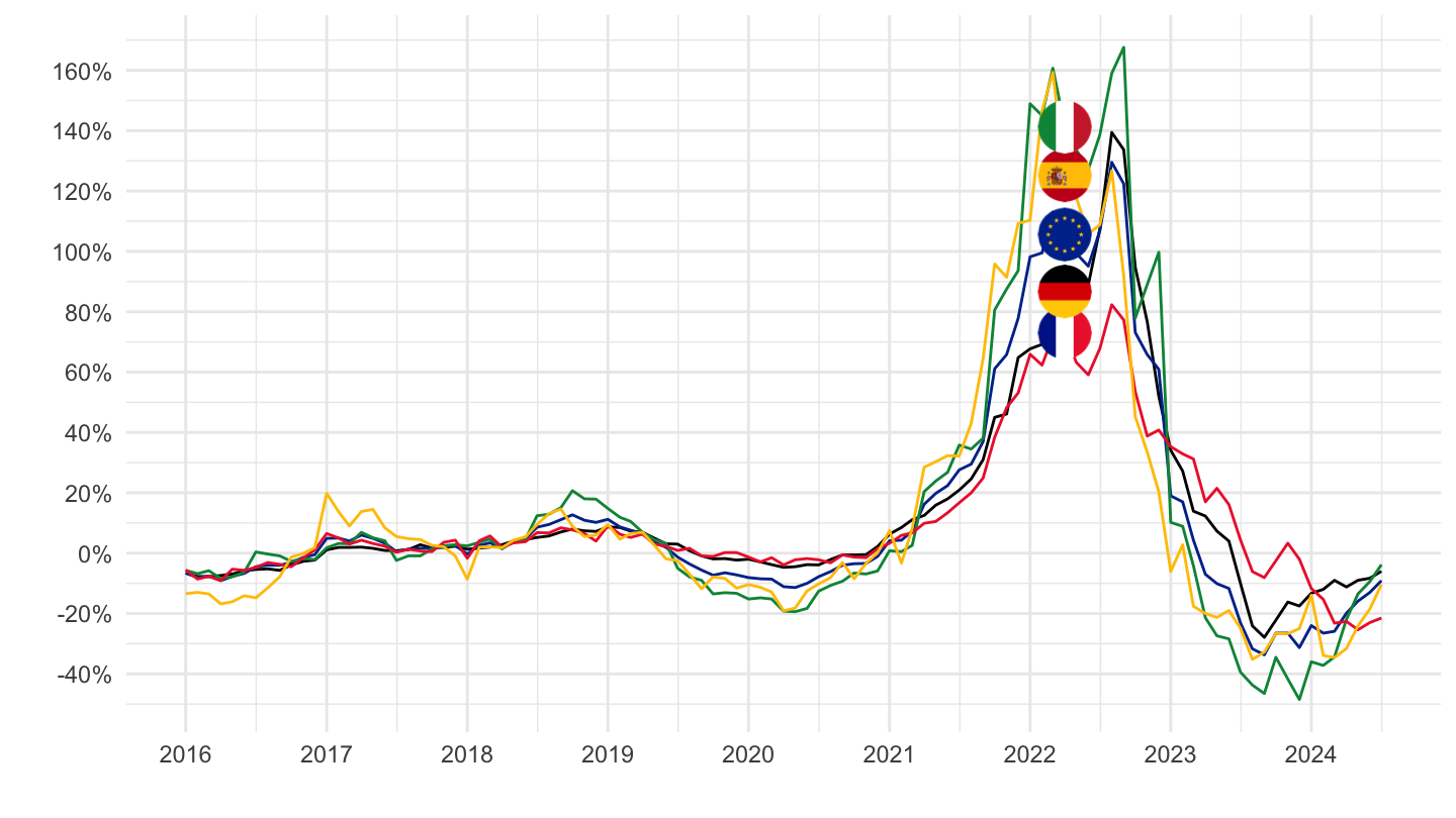
2020-
Code
sts_inppd_m %>%
  filter(nace_r2 == "D35",
         unit == "PCH_SM",
         geo %in% c("FR", "DE", "ES", "IT", "EA19")) %>%
  month_to_date %>%
  filter(date >= as.Date("2020-01-01")) %>%
  left_join(geo, by = "geo") %>%
  mutate(Geo = ifelse(geo == "EA19", "Europe", Geo)) %>%
  left_join(colors, by = c("Geo" = "country")) %>%
  mutate(values = values/100) %>%
  ggplot(.) + geom_line(aes(x = date, y = values, color = color)) +
  theme_minimal() + xlab("") + ylab("") +
  scale_x_date(breaks = seq.Date(as.Date("2019-12-01"), as.Date("2024-01-01"), "3 months"),
               labels = date_format("%b %y")) +
  scale_y_continuous(breaks = 0.01*seq(-100, 200, 20),
                     labels = percent_format(a = 1)) +
  scale_color_identity() + add_5flags +
  theme(legend.position = c(0.75, 0.90),
        legend.title = element_blank())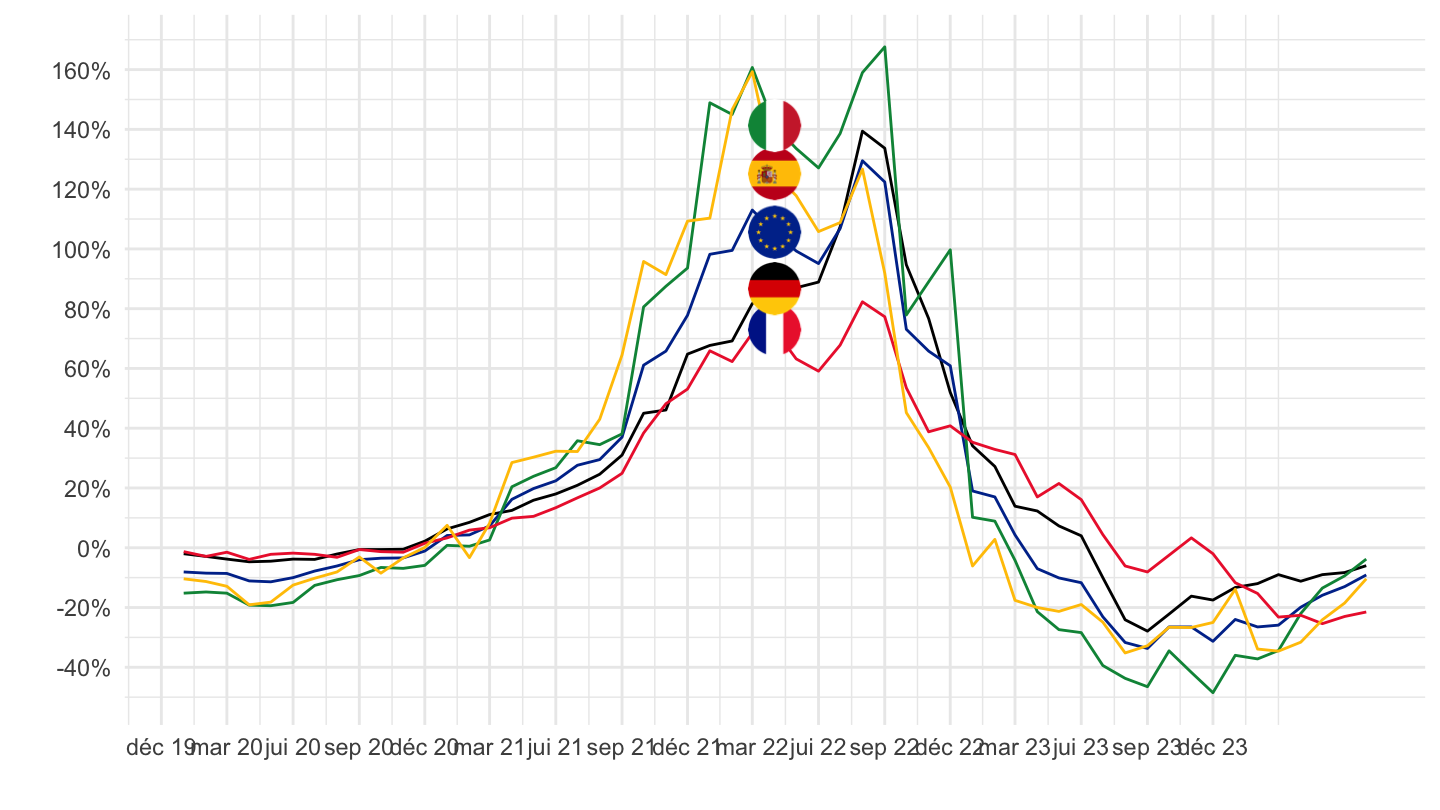
MIG_COG - Consumer Goods
All
Code
sts_inppd_m %>%
  filter(nace_r2 == "MIG_COG",
         unit == "PCH_SM",
         geo %in% c("FR", "DE", "ES", "IT", "EA19")) %>%
  month_to_date %>%
  left_join(geo, by = "geo") %>%
  mutate(Geo = ifelse(geo == "EA19", "Europe", Geo)) %>%
  left_join(colors, by = c("Geo" = "country")) %>%
  mutate(values = values/100) %>%
  ggplot(.) + geom_line(aes(x = date, y = values, color = color)) +
  theme_minimal() + xlab("") + ylab("") +
  scale_x_date(breaks = seq(1960, 2050, 5) %>% paste0("-01-01") %>% as.Date,
               labels = date_format("%Y")) +
  scale_y_continuous(breaks = 0.01*seq(-100, 100, 5),
                     labels = percent_format(a = 1)) +
  scale_color_identity() + add_5flags +
  theme(legend.position = c(0.75, 0.90),
        legend.title = element_blank())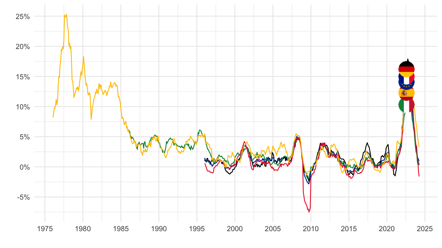
1995-
Code
sts_inppd_m %>%
  filter(nace_r2 == "MIG_COG",
         unit == "PCH_SM",
         geo %in% c("FR", "DE", "ES", "IT", "EA19")) %>%
  month_to_date %>%
  filter(date >= as.Date("1995-01-01")) %>%
  left_join(geo, by = "geo") %>%
  mutate(Geo = ifelse(geo == "EA19", "Europe", Geo)) %>%
  left_join(colors, by = c("Geo" = "country")) %>%
  mutate(values = values/100) %>%
  ggplot(.) + geom_line(aes(x = date, y = values, color = color)) +
  theme_minimal() + xlab("") + ylab("") +
  scale_x_date(breaks = seq(1960, 2050, 5) %>% paste0("-01-01") %>% as.Date,
               labels = date_format("%Y")) +
  scale_y_continuous(breaks = 0.01*seq(-20, 100, 5),
                     labels = percent_format(a = 1)) +
  scale_color_identity() + add_5flags +
  theme(legend.position = c(0.75, 0.90),
        legend.title = element_blank())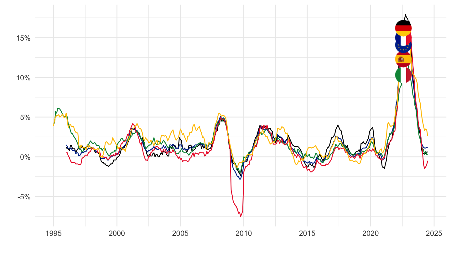
2016-
Code
sts_inppd_m %>%
  filter(nace_r2 == "MIG_COG",
         unit == "PCH_SM",
         geo %in% c("FR", "DE", "ES", "IT", "EA19")) %>%
  month_to_date %>%
  filter(date >= as.Date("2016-01-01")) %>%
  left_join(geo, by = "geo") %>%
  mutate(Geo = ifelse(geo == "EA19", "Europe", Geo)) %>%
  left_join(colors, by = c("Geo" = "country")) %>%
  mutate(values = values/100) %>%
  ggplot(.) + geom_line(aes(x = date, y = values, color = color)) +
  theme_minimal() + xlab("") + ylab("") +
  scale_x_date(breaks = seq(1960, 2050, 1) %>% paste0("-01-01") %>% as.Date,
               labels = date_format("%Y")) +
  scale_y_continuous(breaks = 0.01*seq(-20, 100, 5),
                     labels = percent_format(a = 1)) +
  scale_color_identity() + add_5flags +
  theme(legend.position = c(0.75, 0.90),
        legend.title = element_blank())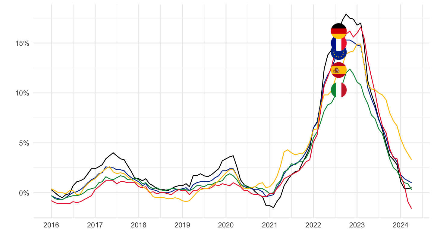
2020-
Code
sts_inppd_m %>%
  filter(nace_r2 == "MIG_COG",
         unit == "PCH_SM",
         geo %in% c("FR", "DE", "ES", "IT", "EA19")) %>%
  month_to_date %>%
  filter(date >= as.Date("2020-01-01")) %>%
  left_join(geo, by = "geo") %>%
  mutate(Geo = ifelse(geo == "EA19", "Europe", Geo)) %>%
  left_join(colors, by = c("Geo" = "country")) %>%
  mutate(values = values/100) %>%
  ggplot(.) + geom_line(aes(x = date, y = values, color = color)) +
  theme_minimal() + xlab("") + ylab("") +
  scale_x_date(breaks = seq.Date(as.Date("2019-12-01"), as.Date("2024-01-01"), "3 months"),
               labels = date_format("%b %y")) +
  scale_y_continuous(breaks = 0.01*seq(-20, 100, 2),
                     labels = percent_format(a = 1)) +
  scale_color_identity() + add_5flags +
  theme(legend.position = c(0.75, 0.90),
        legend.title = element_blank())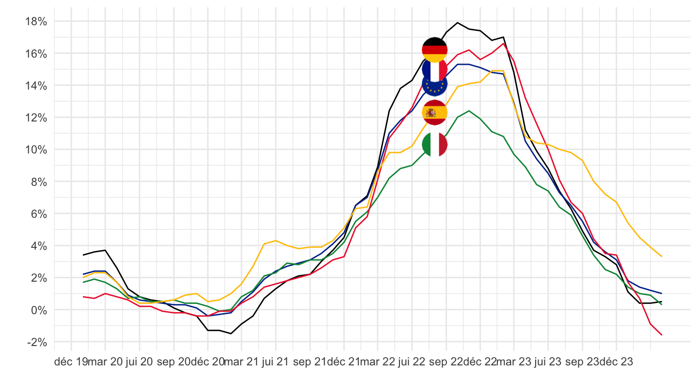
MIG_CAG - Capital Goods
All
Code
sts_inppd_m %>%
  filter(nace_r2 == "MIG_CAG",
         unit == "PCH_SM",
         geo %in% c("FR", "DE", "ES", "IT", "EA19")) %>%
  month_to_date %>%
  left_join(geo, by = "geo") %>%
  mutate(Geo = ifelse(geo == "EA19", "Europe", Geo)) %>%
  left_join(colors, by = c("Geo" = "country")) %>%
  mutate(values = values/100) %>%
  ggplot(.) + geom_line(aes(x = date, y = values, color = color)) +
  theme_minimal() + xlab("") + ylab("") +
  scale_x_date(breaks = seq(1960, 2050, 5) %>% paste0("-01-01") %>% as.Date,
               labels = date_format("%Y")) +
  scale_y_continuous(breaks = 0.01*seq(-100, 100, 5),
                     labels = percent_format(a = 1)) +
  scale_color_identity() + add_5flags +
  theme(legend.position = c(0.75, 0.90),
        legend.title = element_blank())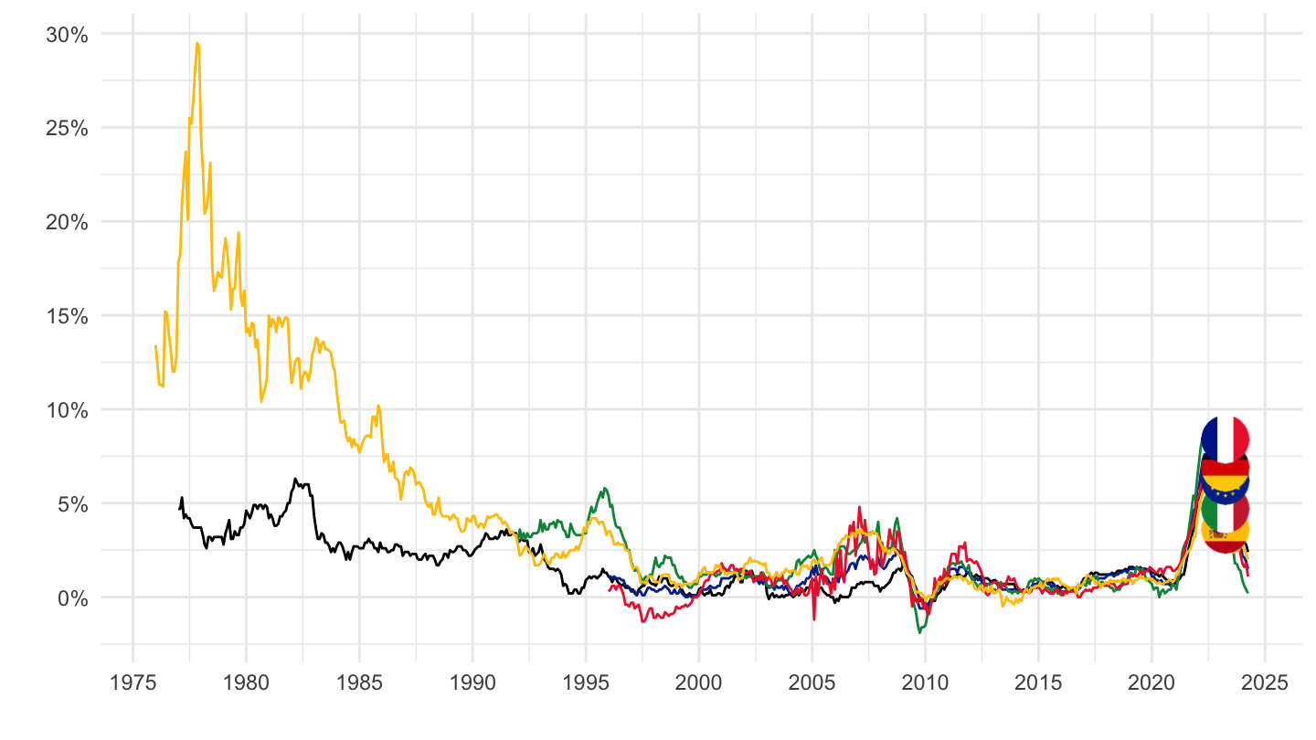
1995-
Code
sts_inppd_m %>%
  filter(nace_r2 == "MIG_CAG",
         unit == "PCH_SM",
         geo %in% c("FR", "DE", "ES", "IT", "EA19")) %>%
  month_to_date %>%
  filter(date >= as.Date("1995-01-01")) %>%
  left_join(geo, by = "geo") %>%
  mutate(Geo = ifelse(geo == "EA19", "Europe", Geo)) %>%
  left_join(colors, by = c("Geo" = "country")) %>%
  mutate(values = values/100) %>%
  ggplot(.) + geom_line(aes(x = date, y = values, color = color)) +
  theme_minimal() + xlab("") + ylab("") +
  scale_x_date(breaks = seq(1960, 2050, 5) %>% paste0("-01-01") %>% as.Date,
               labels = date_format("%Y")) +
  scale_y_continuous(breaks = 0.01*seq(-20, 100, 5),
                     labels = percent_format(a = 1)) +
  scale_color_identity() + add_5flags +
  theme(legend.position = c(0.75, 0.90),
        legend.title = element_blank())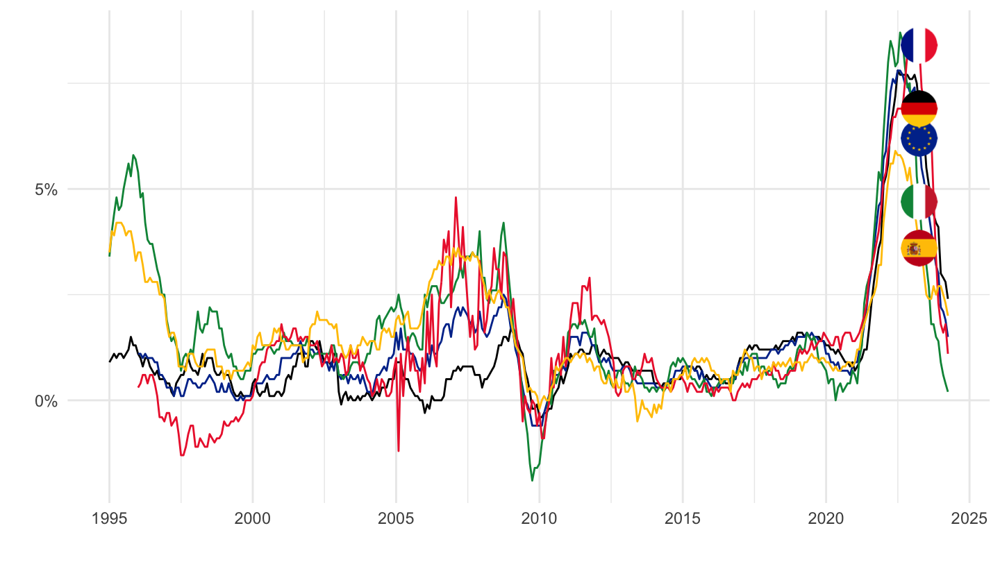
2016-
Code
sts_inppd_m %>%
  filter(nace_r2 == "MIG_CAG",
         unit == "PCH_SM",
         geo %in% c("FR", "DE", "ES", "IT", "EA19")) %>%
  month_to_date %>%
  filter(date >= as.Date("2016-01-01")) %>%
  left_join(geo, by = "geo") %>%
  mutate(Geo = ifelse(geo == "EA19", "Europe", Geo)) %>%
  left_join(colors, by = c("Geo" = "country")) %>%
  mutate(values = values/100) %>%
  ggplot(.) + geom_line(aes(x = date, y = values, color = color)) +
  theme_minimal() + xlab("") + ylab("") +
  scale_x_date(breaks = seq(1960, 2050, 1) %>% paste0("-01-01") %>% as.Date,
               labels = date_format("%Y")) +
  scale_y_continuous(breaks = 0.01*seq(-20, 100, 5),
                     labels = percent_format(a = 1)) +
  scale_color_identity() + add_5flags +
  theme(legend.position = c(0.75, 0.90),
        legend.title = element_blank())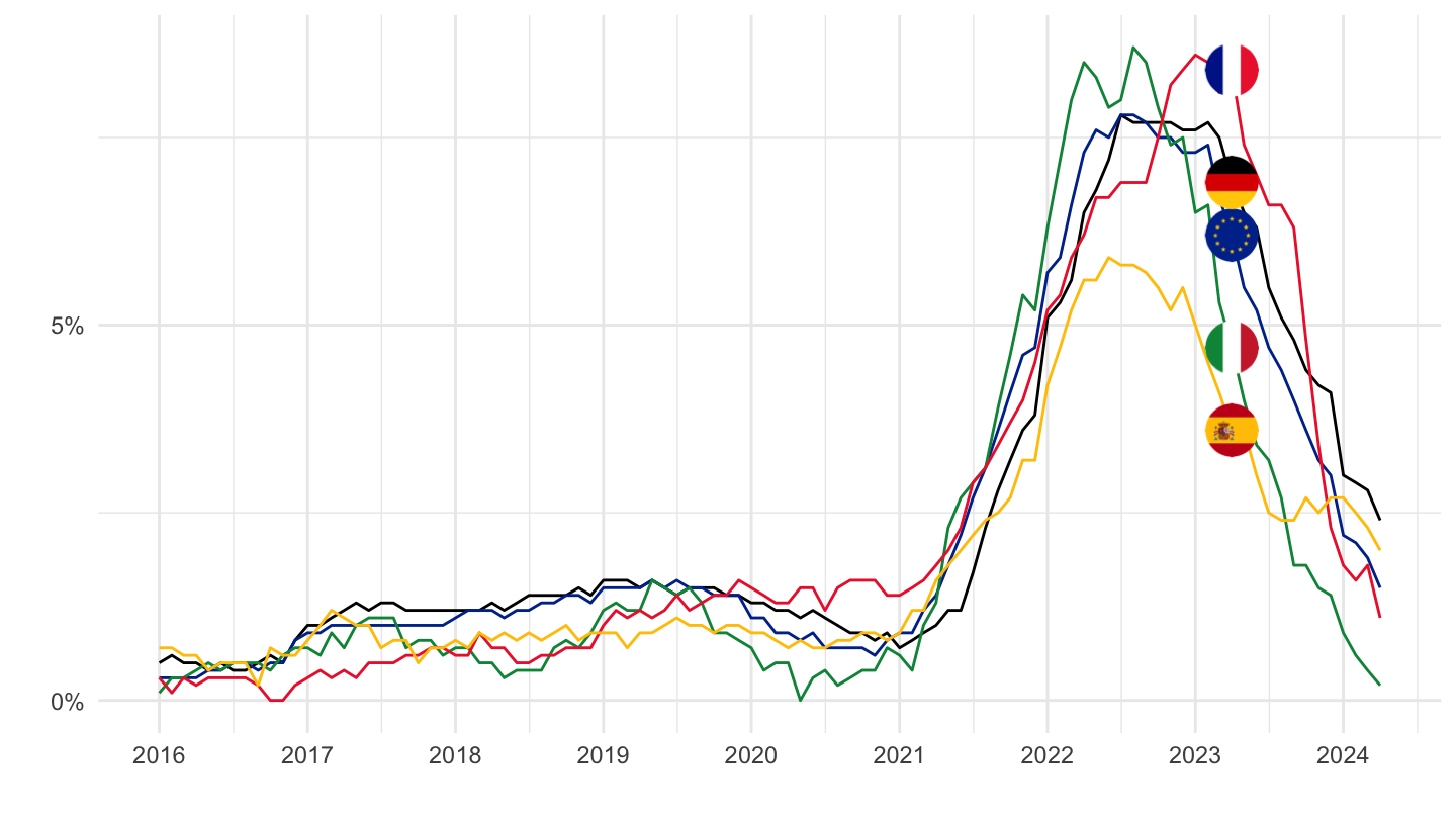
2020-
Code
sts_inppd_m %>%
  filter(nace_r2 == "MIG_CAG",
         unit == "PCH_SM",
         geo %in% c("FR", "DE", "ES", "IT", "EA19")) %>%
  month_to_date %>%
  filter(date >= as.Date("2020-01-01")) %>%
  left_join(geo, by = "geo") %>%
  mutate(Geo = ifelse(geo == "EA19", "Europe", Geo)) %>%
  left_join(colors, by = c("Geo" = "country")) %>%
  mutate(values = values/100) %>%
  ggplot(.) + geom_line(aes(x = date, y = values, color = color)) +
  theme_minimal() + xlab("") + ylab("") +
  scale_x_date(breaks = seq.Date(as.Date("2019-12-01"), as.Date("2024-01-01"), "3 months"),
               labels = date_format("%b %y")) +
  scale_y_continuous(breaks = 0.01*seq(-20, 100, 2),
                     labels = percent_format(a = 1)) +
  scale_color_identity() + add_5flags +
  theme(legend.position = c(0.75, 0.90),
        legend.title = element_blank())
MIG_NRG - Energy
All
Code
sts_inppd_m %>%
  filter(nace_r2 == "MIG_NRG",
         unit == "PCH_SM",
         geo %in% c("FR", "DE", "ES", "IT", "EA19")) %>%
  month_to_date %>%
  left_join(geo, by = "geo") %>%
  mutate(Geo = ifelse(geo == "EA19", "Europe", Geo)) %>%
  left_join(colors, by = c("Geo" = "country")) %>%
  mutate(values = values/100) %>%
  ggplot(.) + geom_line(aes(x = date, y = values, color = color)) +
  theme_minimal() + xlab("") + ylab("") +
  scale_x_date(breaks = seq(1960, 2050, 5) %>% paste0("-01-01") %>% as.Date,
               labels = date_format("%Y")) +
  scale_y_continuous(breaks = 0.01*seq(-20, 200, 10),
                     labels = percent_format(a = 1)) +
  scale_color_identity() + add_5flags +
  theme(legend.position = c(0.75, 0.90),
        legend.title = element_blank())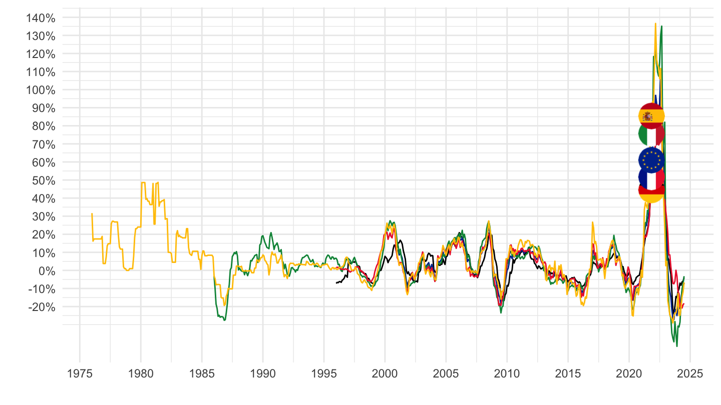
1995-
Code
sts_inppd_m %>%
  filter(nace_r2 == "MIG_NRG",
         unit == "PCH_SM",
         geo %in% c("FR", "DE", "ES", "IT", "EA19")) %>%
  month_to_date %>%
  filter(date >= as.Date("1995-01-01")) %>%
  left_join(geo, by = "geo") %>%
  mutate(Geo = ifelse(geo == "EA19", "Europe", Geo)) %>%
  left_join(colors, by = c("Geo" = "country")) %>%
  mutate(values = values/100) %>%
  ggplot(.) + geom_line(aes(x = date, y = values, color = color)) +
  theme_minimal() + xlab("") + ylab("") +
  scale_x_date(breaks = seq(1960, 2050, 5) %>% paste0("-01-01") %>% as.Date,
               labels = date_format("%Y")) +
  scale_y_continuous(breaks = 0.01*seq(-20, 200, 10),
                     labels = percent_format(a = 1)) +
  scale_color_identity() + add_5flags +
  theme(legend.position = c(0.75, 0.90),
        legend.title = element_blank())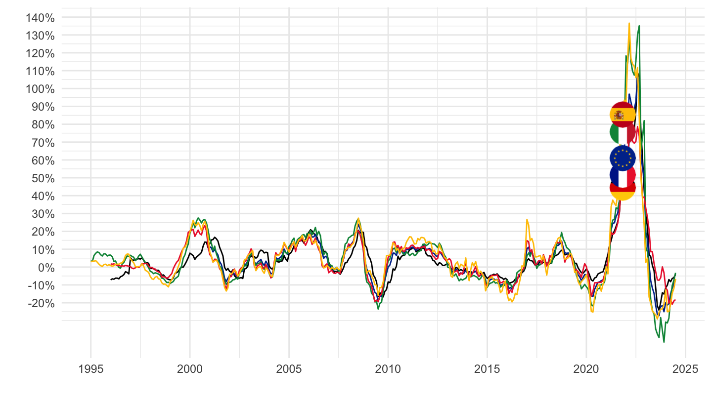
2016-
Code
sts_inppd_m %>%
  filter(nace_r2 == "MIG_NRG",
         unit == "PCH_SM",
         geo %in% c("FR", "DE", "ES", "IT", "EA19")) %>%
  month_to_date %>%
  filter(date >= as.Date("2016-01-01")) %>%
  left_join(geo, by = "geo") %>%
  mutate(Geo = ifelse(geo == "EA19", "Europe", Geo)) %>%
  left_join(colors, by = c("Geo" = "country")) %>%
  mutate(values = values/100) %>%
  ggplot(.) + geom_line(aes(x = date, y = values, color = color)) +
  theme_minimal() + xlab("") + ylab("") +
  scale_x_date(breaks = seq(1960, 2050, 1) %>% paste0("-01-01") %>% as.Date,
               labels = date_format("%Y")) +
  scale_y_continuous(breaks = 0.01*seq(-20, 200, 10),
                     labels = percent_format(a = 1)) +
  scale_color_identity() + add_5flags +
  theme(legend.position = c(0.75, 0.90),
        legend.title = element_blank())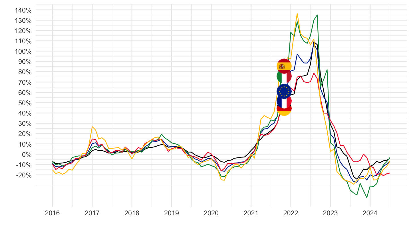
2020-
Code
sts_inppd_m %>%
  filter(nace_r2 == "MIG_NRG",
         unit == "PCH_SM",
         geo %in% c("FR", "DE", "ES", "IT", "EA19")) %>%
  month_to_date %>%
  filter(date >= as.Date("2020-01-01")) %>%
  left_join(geo, by = "geo") %>%
  mutate(Geo = ifelse(geo == "EA19", "Europe", Geo)) %>%
  left_join(colors, by = c("Geo" = "country")) %>%
  mutate(values = values/100) %>%
  ggplot(.) + geom_line(aes(x = date, y = values, color = color)) +
  theme_minimal() + xlab("") + ylab("") +
  scale_x_date(breaks = seq.Date(as.Date("2019-12-01"), as.Date("2024-01-01"), "3 months"),
               labels = date_format("%b %y")) +
  scale_y_continuous(breaks = 0.01*seq(-20, 200, 10),
                     labels = percent_format(a = 1)) +
  scale_color_identity() + add_5flags +
  theme(legend.position = c(0.75, 0.90),
        legend.title = element_blank())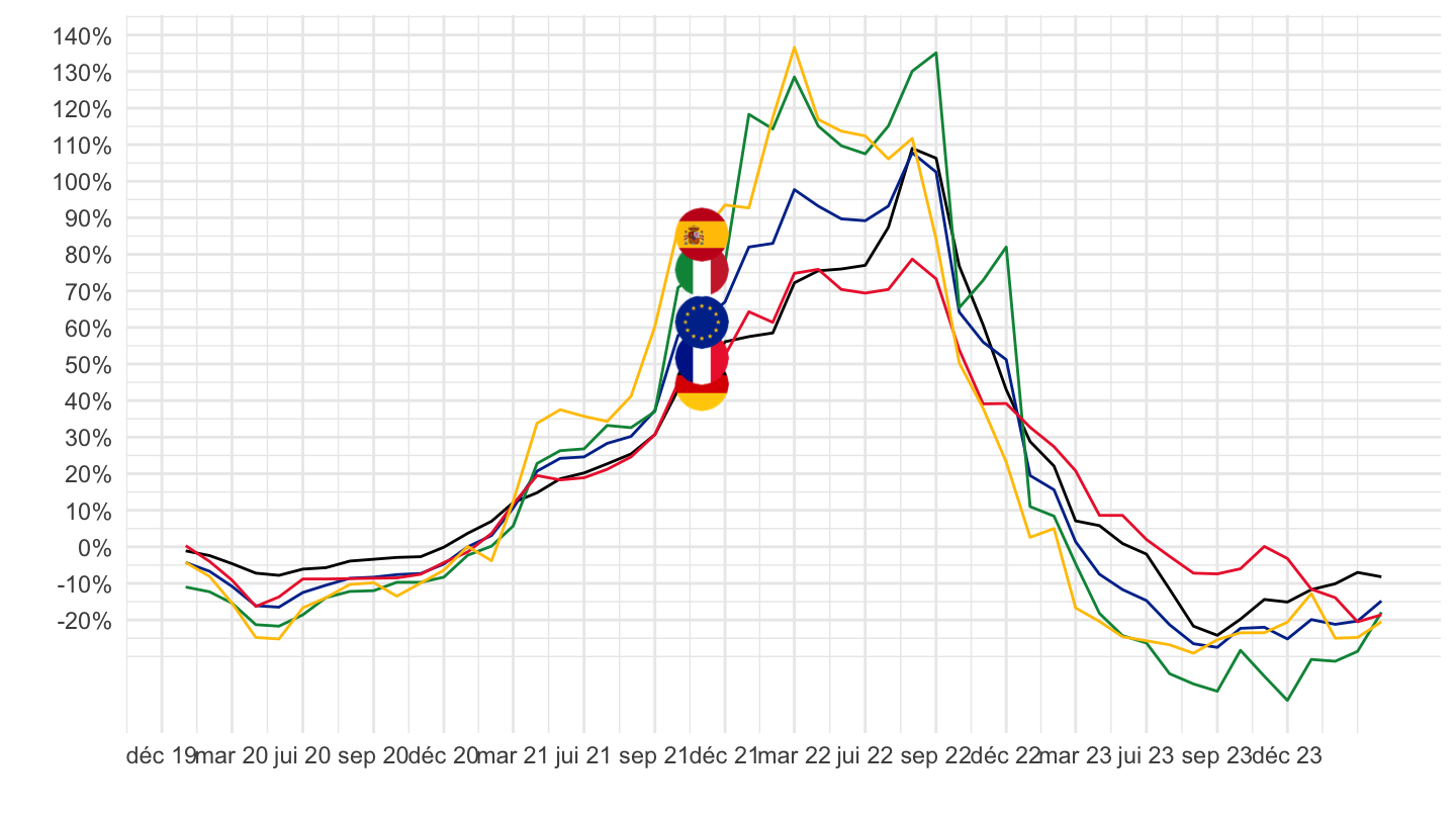
MIG_ING - Intermediate goods
All
Code
sts_inppd_m %>%
  filter(nace_r2 == "MIG_ING",
         unit == "PCH_SM",
         geo %in% c("FR", "DE", "ES", "IT", "EA19")) %>%
  month_to_date %>%
  left_join(geo, by = "geo") %>%
  mutate(Geo = ifelse(geo == "EA19", "Europe", Geo)) %>%
  left_join(colors, by = c("Geo" = "country")) %>%
  mutate(values = values/100) %>%
  ggplot(.) + geom_line(aes(x = date, y = values, color = color)) +
  theme_minimal() + xlab("") + ylab("") +
  scale_x_date(breaks = seq(1960, 2050, 5) %>% paste0("-01-01") %>% as.Date,
               labels = date_format("%Y")) +
  scale_y_continuous(breaks = 0.01*seq(-100, 100, 5),
                     labels = percent_format(a = 1)) +
  scale_color_identity() + add_5flags +
  theme(legend.position = c(0.75, 0.90),
        legend.title = element_blank())
1995-
Code
sts_inppd_m %>%
  filter(nace_r2 == "MIG_ING",
         unit == "PCH_SM",
         geo %in% c("FR", "DE", "ES", "IT", "EA19")) %>%
  month_to_date %>%
  filter(date >= as.Date("1995-01-01")) %>%
  left_join(geo, by = "geo") %>%
  mutate(Geo = ifelse(geo == "EA19", "Europe", Geo)) %>%
  left_join(colors, by = c("Geo" = "country")) %>%
  mutate(values = values/100) %>%
  ggplot(.) + geom_line(aes(x = date, y = values, color = color)) +
  theme_minimal() + xlab("") + ylab("") +
  scale_x_date(breaks = seq(1960, 2050, 5) %>% paste0("-01-01") %>% as.Date,
               labels = date_format("%Y")) +
  scale_y_continuous(breaks = 0.01*seq(-20, 200, 10),
                     labels = percent_format(a = 1)) +
  scale_color_identity() + add_5flags +
  theme(legend.position = c(0.75, 0.90),
        legend.title = element_blank())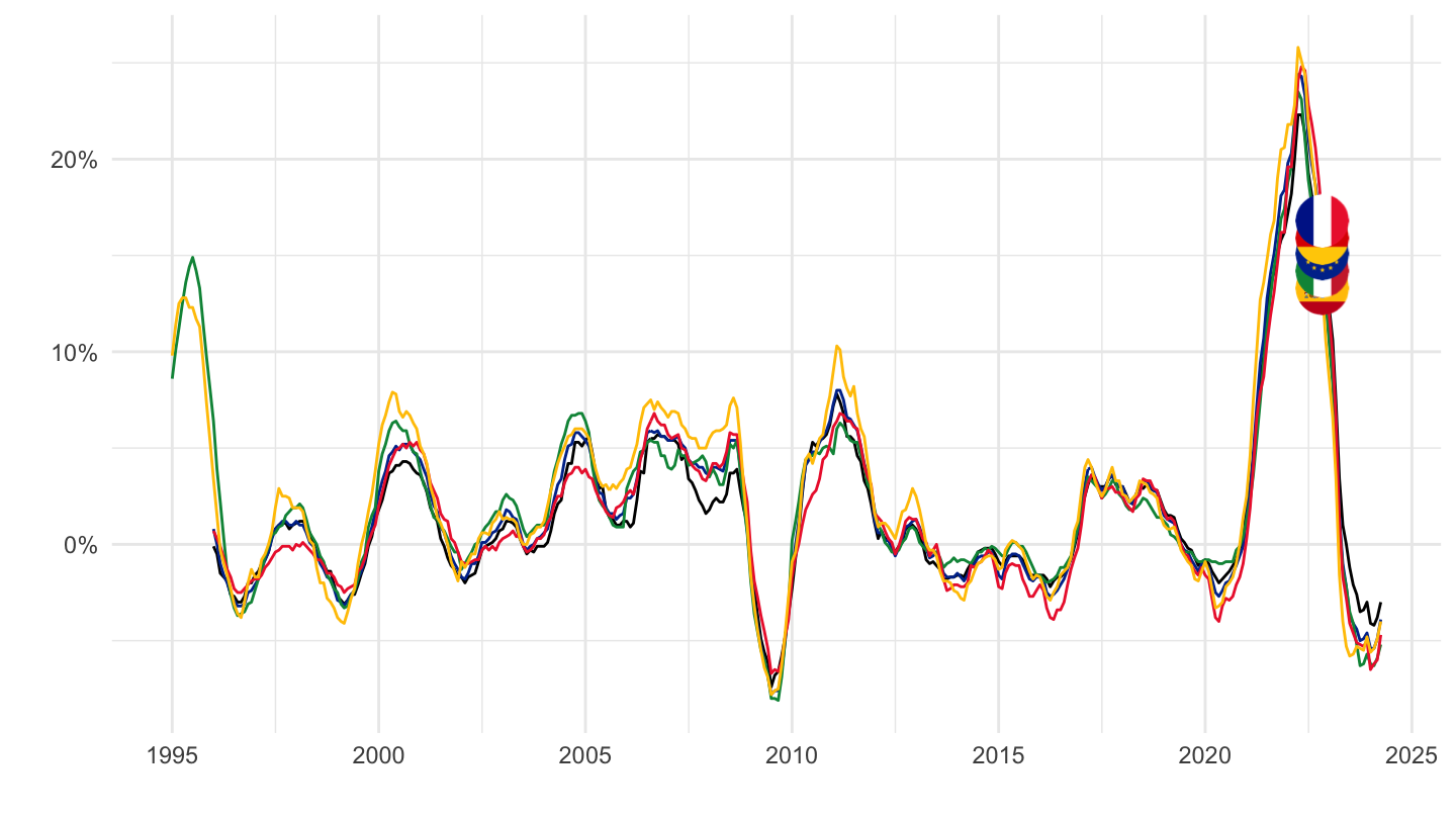
2016-
Code
sts_inppd_m %>%
  filter(nace_r2 == "MIG_ING",
         unit == "PCH_SM",
         geo %in% c("FR", "DE", "ES", "IT", "EA19")) %>%
  month_to_date %>%
  filter(date >= as.Date("2016-01-01")) %>%
  left_join(geo, by = "geo") %>%
  mutate(Geo = ifelse(geo == "EA19", "Europe", Geo)) %>%
  left_join(colors, by = c("Geo" = "country")) %>%
  mutate(values = values/100) %>%
  ggplot(.) + geom_line(aes(x = date, y = values, color = color)) +
  theme_minimal() + xlab("") + ylab("") +
  scale_x_date(breaks = seq(1960, 2050, 1) %>% paste0("-01-01") %>% as.Date,
               labels = date_format("%Y")) +
  scale_y_continuous(breaks = 0.01*seq(-20, 200, 10),
                     labels = percent_format(a = 1)) +
  scale_color_identity() + add_5flags +
  theme(legend.position = c(0.75, 0.90),
        legend.title = element_blank())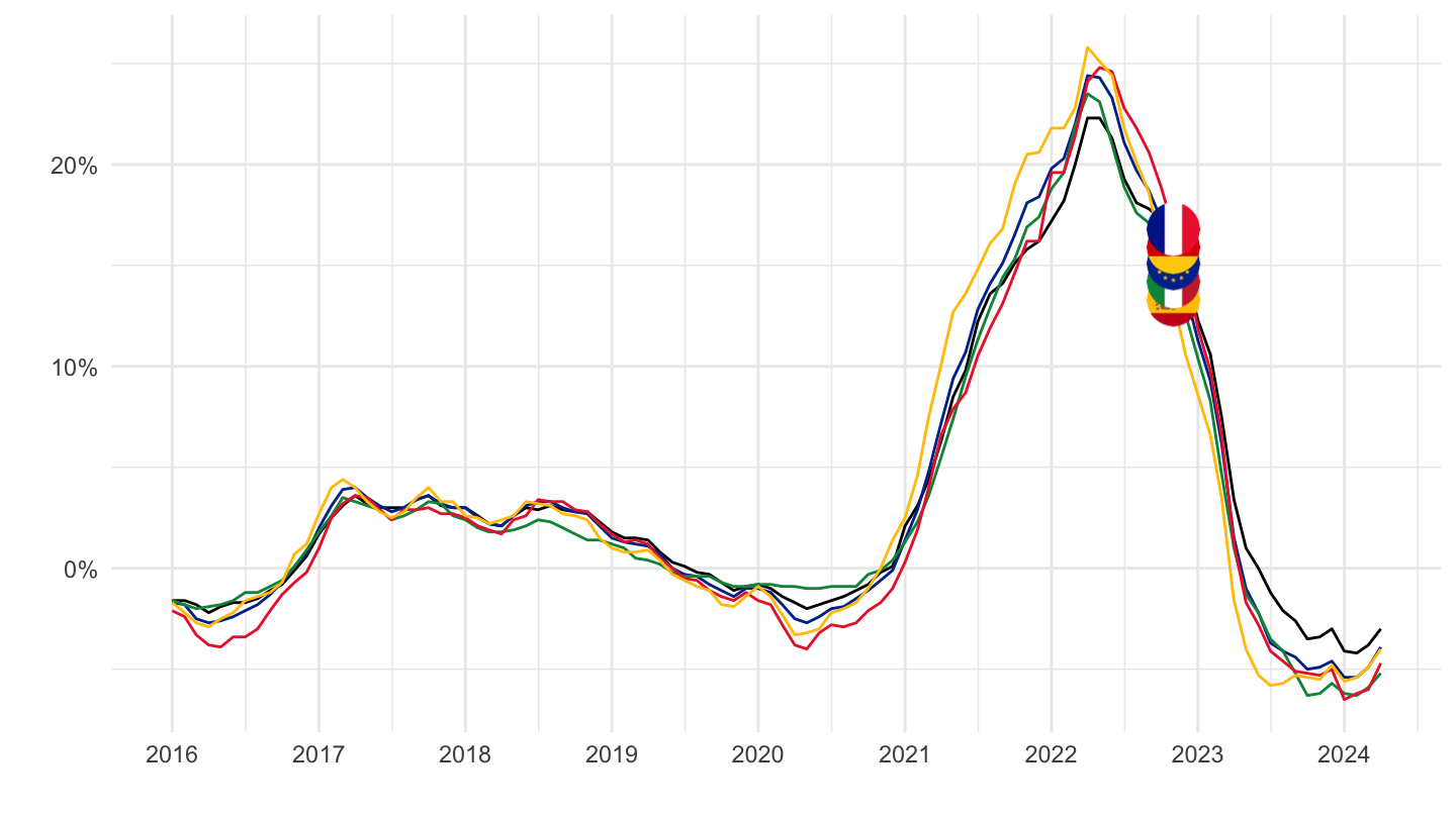
2020-
Code
sts_inppd_m %>%
  filter(nace_r2 == "MIG_ING",
         unit == "PCH_SM",
         geo %in% c("FR", "DE", "ES", "IT", "EA19")) %>%
  month_to_date %>%
  filter(date >= as.Date("2020-01-01")) %>%
  left_join(geo, by = "geo") %>%
  mutate(Geo = ifelse(geo == "EA19", "Europe", Geo)) %>%
  left_join(colors, by = c("Geo" = "country")) %>%
  mutate(values = values/100) %>%
  ggplot(.) + geom_line(aes(x = date, y = values, color = color)) +
  theme_minimal() + xlab("") + ylab("") +
  scale_x_date(breaks = seq.Date(as.Date("2019-12-01"), as.Date("2024-01-01"), "3 months"),
               labels = date_format("%b %y")) +
  scale_y_continuous(breaks = 0.01*seq(-20, 200, 10),
                     labels = percent_format(a = 1)) +
  scale_color_identity() + add_5flags +
  theme(legend.position = c(0.75, 0.90),
        legend.title = element_blank())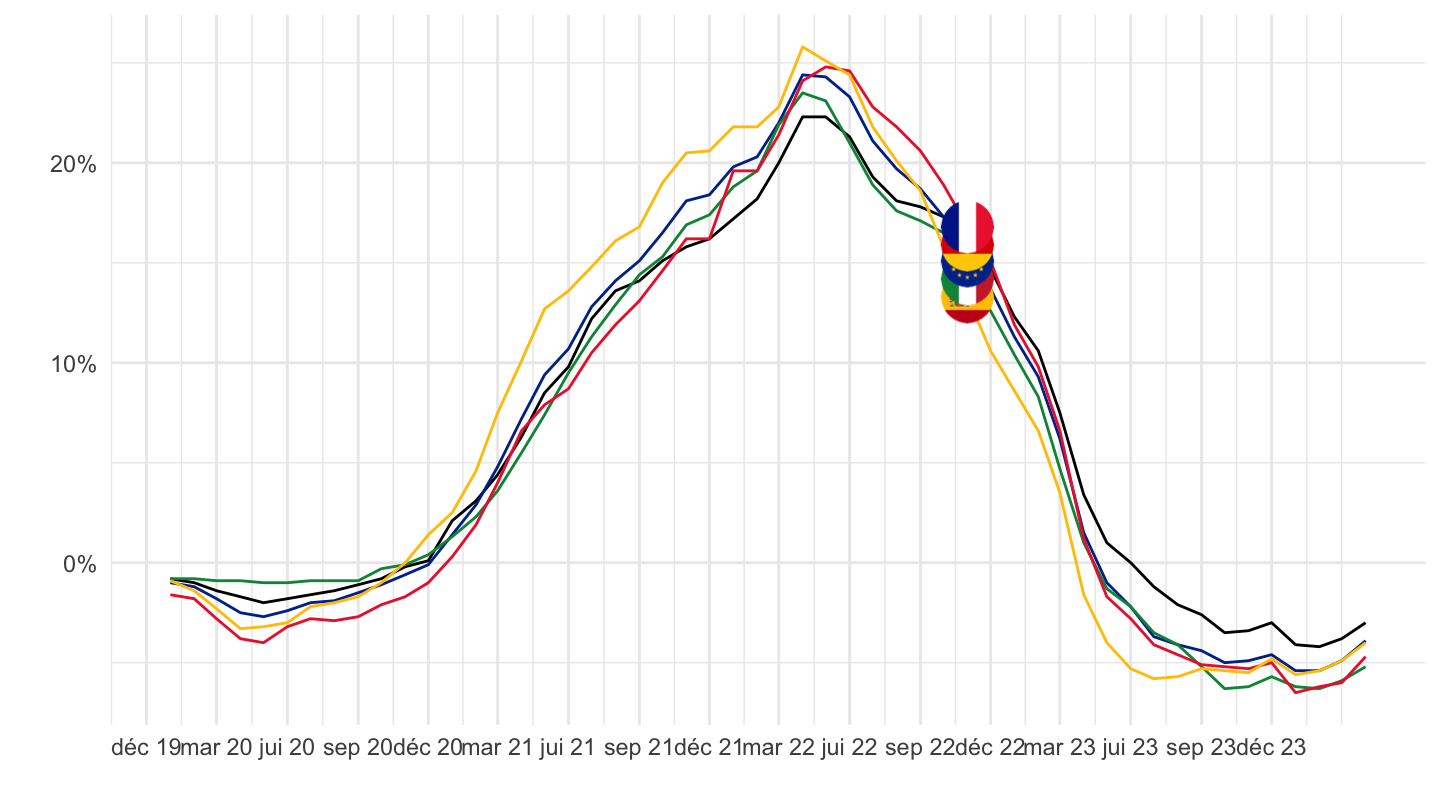
MIG_NDCOG - Non-durable consumer goods
All
Code
sts_inppd_m %>%
  filter(nace_r2 == "MIG_NDCOG",
         unit == "PCH_SM",
         geo %in% c("FR", "DE", "ES", "IT", "EA19")) %>%
  month_to_date %>%
  left_join(geo, by = "geo") %>%
  mutate(Geo = ifelse(geo == "EA19", "Europe", Geo)) %>%
  left_join(colors, by = c("Geo" = "country")) %>%
  mutate(values = values/100) %>%
  ggplot(.) + geom_line(aes(x = date, y = values, color = color)) +
  theme_minimal() + xlab("") + ylab("") +
  scale_x_date(breaks = seq(1960, 2050, 5) %>% paste0("-01-01") %>% as.Date,
               labels = date_format("%Y")) +
  scale_y_continuous(breaks = 0.01*seq(-100, 100, 5),
                     labels = percent_format(a = 1)) +
  scale_color_identity() + add_5flags +
  theme(legend.position = c(0.75, 0.90),
        legend.title = element_blank())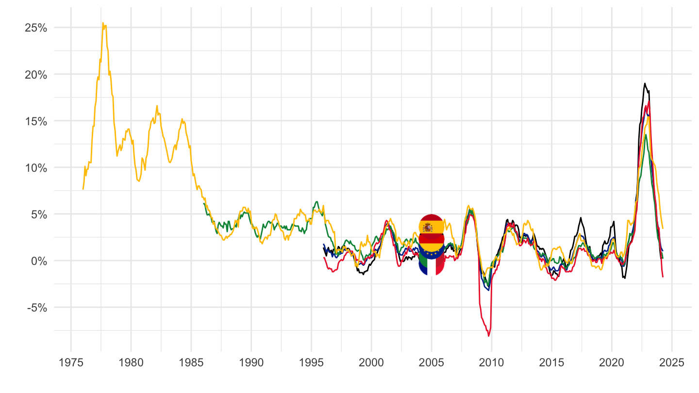
1995-
Code
sts_inppd_m %>%
  filter(nace_r2 == "MIG_NDCOG",
         unit == "PCH_SM",
         geo %in% c("FR", "DE", "ES", "IT", "EA19")) %>%
  month_to_date %>%
  filter(date >= as.Date("1995-01-01")) %>%
  left_join(geo, by = "geo") %>%
  mutate(Geo = ifelse(geo == "EA19", "Europe", Geo)) %>%
  left_join(colors, by = c("Geo" = "country")) %>%
  mutate(values = values/100) %>%
  ggplot(.) + geom_line(aes(x = date, y = values, color = color)) +
  theme_minimal() + xlab("") + ylab("") +
  scale_x_date(breaks = seq(1960, 2050, 5) %>% paste0("-01-01") %>% as.Date,
               labels = date_format("%Y")) +
  scale_y_continuous(breaks = 0.01*seq(-20, 200, 2),
                     labels = percent_format(a = 1)) +
  scale_color_identity() + add_5flags +
  theme(legend.position = c(0.75, 0.90),
        legend.title = element_blank())
2016-
Code
sts_inppd_m %>%
  filter(nace_r2 == "MIG_NDCOG",
         unit == "PCH_SM",
         geo %in% c("FR", "DE", "ES", "IT", "EA19")) %>%
  month_to_date %>%
  filter(date >= as.Date("2016-01-01")) %>%
  left_join(geo, by = "geo") %>%
  mutate(Geo = ifelse(geo == "EA19", "Europe", Geo)) %>%
  left_join(colors, by = c("Geo" = "country")) %>%
  mutate(values = values/100) %>%
  ggplot(.) + geom_line(aes(x = date, y = values, color = color)) +
  theme_minimal() + xlab("") + ylab("") +
  scale_x_date(breaks = seq(1960, 2050, 1) %>% paste0("-01-01") %>% as.Date,
               labels = date_format("%Y")) +
  scale_y_continuous(breaks = 0.01*seq(-20, 200, 2),
                     labels = percent_format(a = 1)) +
  scale_color_identity() + add_5flags +
  theme(legend.position = c(0.75, 0.90),
        legend.title = element_blank())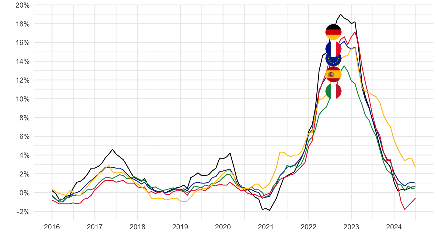
2020-
Code
sts_inppd_m %>%
  filter(nace_r2 == "MIG_NDCOG",
         unit == "PCH_SM",
         geo %in% c("FR", "DE", "ES", "IT", "EA19")) %>%
  month_to_date %>%
  filter(date >= as.Date("2020-01-01")) %>%
  left_join(geo, by = "geo") %>%
  mutate(Geo = ifelse(geo == "EA19", "Europe", Geo)) %>%
  left_join(colors, by = c("Geo" = "country")) %>%
  mutate(values = values/100) %>%
  ggplot(.) + geom_line(aes(x = date, y = values, color = color)) +
  theme_minimal() + xlab("") + ylab("") +
  scale_x_date(breaks = seq.Date(as.Date("2019-12-01"), as.Date("2024-01-01"), "3 months"),
               labels = date_format("%b %y")) +
  scale_y_continuous(breaks = 0.01*seq(-20, 200, 2),
                     labels = percent_format(a = 1)) +
  scale_color_identity() + add_5flags +
  theme(legend.position = c(0.75, 0.90),
        legend.title = element_blank())