Indice pour la révision d’un loyer d’habitation

Données - INSEE

Auteur

François Geerolf

Info

Last observation: 2026-Q2

First observation: 2000-Q1

Number of observations: 356

Last data update: 24 jul 2026, 03:05. Last compile: 24 jul 2026, 06:20

Structure

Last

Code

IRL %>%
  group_by(TIME_PERIOD) %>%
  summarise(Nobs = n()) %>%
  arrange(desc(TIME_PERIOD)) %>%
  head(1) %>%
  print_table_conditional()

TIME_PERIOD	Nobs
2026-Q2	6

Indice

Linear

Tous

Code

IRL %>%
  filter(NATURE == "INDICE") %>%
  quarter_to_date %>%
  ggplot(.) + theme_minimal() + ylab("") + xlab("") +
  geom_line(aes(x = date, y = OBS_VALUE, color = TITLE_FR)) +
  theme(legend.title = element_blank(),
        legend.position = c(0.6, 0.7)) +
  scale_x_date(breaks = seq(1950, 2100, 2) %>% paste0("-01-01") %>% as.Date,
               labels = date_format("%Y")) +
  scale_y_log10(breaks = seq(0, 200, 5))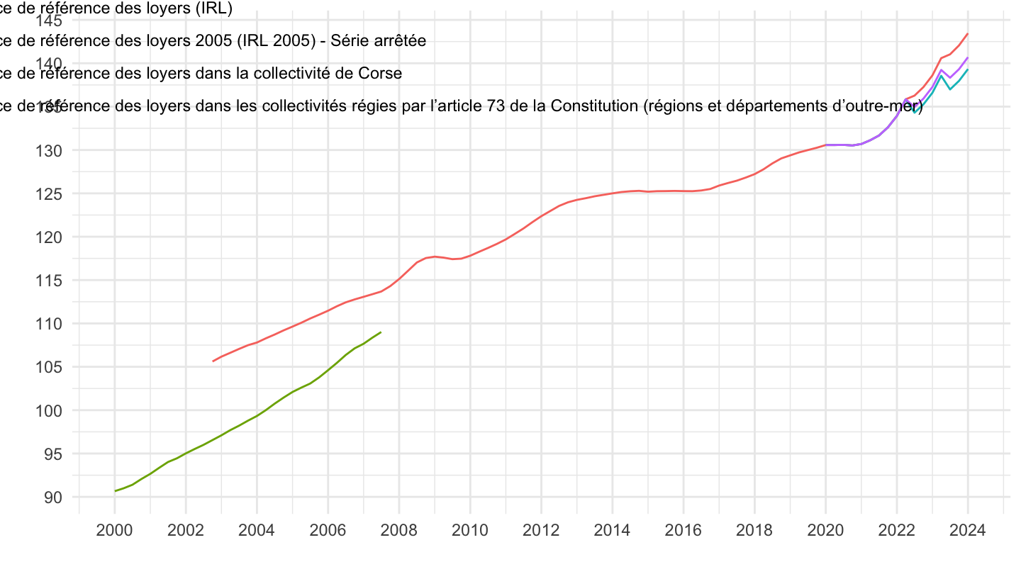

2017-

Code

IRL %>%
  filter(NATURE == "INDICE") %>%
  quarter_to_date %>%
  filter(date >= as.Date("2017-01-01")) %>%
  group_by(TITLE_FR) %>%
  arrange(date) %>%
  mutate(OBS_VALUE = 100*OBS_VALUE/OBS_VALUE[1]) %>%
  ggplot(.) + theme_minimal() + ylab("") + xlab("") +
  geom_line(aes(x = date, y = OBS_VALUE, color = TITLE_FR)) +
  theme(legend.title = element_blank(),
        legend.position = c(0.6, 0.7)) +
  scale_x_date(breaks = seq(1950, 2100, 1) %>% paste0("-01-01") %>% as.Date,
               labels = date_format("%Y")) +
  scale_y_log10(breaks = seq(0, 200, 5)) +
  geom_label(data = . %>% filter(date == max(date)),
             aes(x = date, y = OBS_VALUE, color = TITLE_FR, label = round(OBS_VALUE, 1)),
             show.legend = F)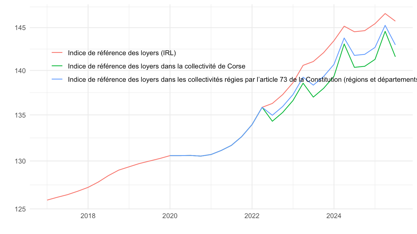

2020-

Code

IRL %>%
  filter(NATURE == "INDICE") %>%
  quarter_to_date %>%
  filter(date >= as.Date("2020-01-01")) %>%
  group_by(TITLE_FR) %>%
  arrange(date) %>%
  mutate(OBS_VALUE = 100*OBS_VALUE/OBS_VALUE[1]) %>%
  ggplot(.) + theme_minimal() + ylab("") + xlab("") +
  geom_line(aes(x = date, y = OBS_VALUE, color = TITLE_FR)) +
  theme(legend.title = element_blank(),
        legend.position = c(0.6, 0.7)) +
  scale_x_date(breaks = seq(1950, 2100, 1) %>% paste0("-01-01") %>% as.Date,
               labels = date_format("%Y")) +
  scale_y_log10(breaks = seq(0, 200, 1)) +
  geom_label(data = . %>% filter(date == max(date)),
             aes(x = date, y = OBS_VALUE, color = TITLE_FR, label = round(OBS_VALUE, 1)),
             show.legend = F)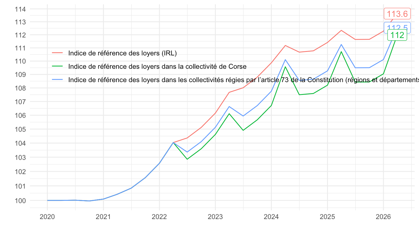

2017-

Code

IRL %>%
  filter(NATURE == "INDICE",
         IDBANK == "001515333") %>%
  quarter_to_date %>%
  filter(date >= as.Date("2017-01-01")) %>%
  arrange(date) %>%
  mutate(OBS_VALUE = 100*OBS_VALUE/OBS_VALUE[1]) %>%
  ggplot(.) + theme_minimal() + ylab("") + xlab("") +
  geom_line(aes(x = date, y = OBS_VALUE)) +
  theme(legend.title = element_blank(),
        legend.position = c(0.2, 0.7)) +
  scale_x_date(breaks = seq(1950, 2100, 1) %>% paste0("-01-01") %>% as.Date,
               labels = date_format("%Y")) +
  scale_y_log10(breaks = seq(0, 200, 2)) +
  geom_label(data = . %>% filter(date == max(date)),
             aes(x = date, y = OBS_VALUE, label = round(OBS_VALUE, 1)),
             show.legend = F)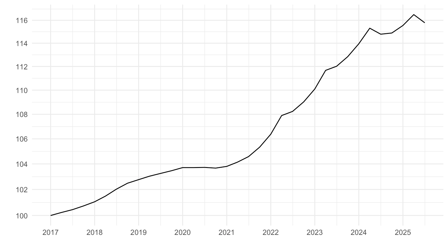

Linear - 4 quarters rolling

Code

IRL %>%
  filter(NATURE == "INDICE") %>%
  quarter_to_date %>%
  group_by(TITLE_FR) %>%
  arrange(date) %>%
  mutate(OBS_VALUE = OBS_VALUE/lag(OBS_VALUE, 4)-1) %>%
  ggplot(.) + theme_minimal() + ylab("") + xlab("") +
  geom_line(aes(x = date, y = OBS_VALUE, color = TITLE_FR)) +
  theme(legend.title = element_blank(),
        legend.position = c(0.65, 0.95)) +
  
  scale_x_date(breaks = seq(1950, 2100, 2) %>% paste0("-01-01") %>% as.Date,
               labels = date_format("%Y")) +
  scale_y_continuous(breaks = 0.01*seq(-100, 300, 0.5),
                     labels = percent_format(accuracy = .1, prefix = ""))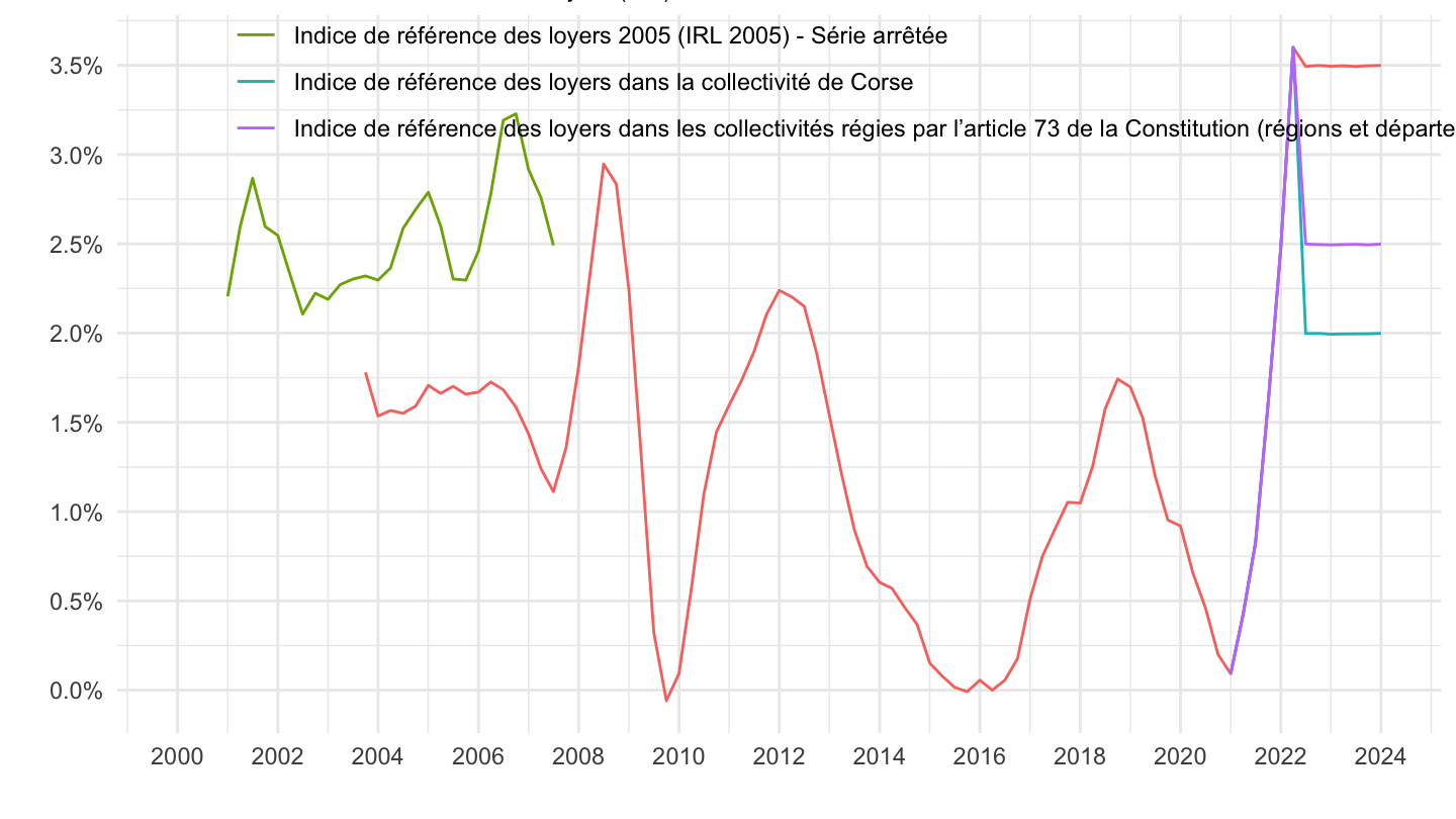

Log

Code

IRL %>%
  filter(NATURE == "INDICE") %>%
  quarter_to_date %>%
  ggplot(.) + theme_minimal() + ylab("") + xlab("") +
  geom_line(aes(x = date, y = OBS_VALUE, color = TITLE_FR)) +
  theme(legend.title = element_blank(),
        legend.position = c(0.38, 0.92)) +
  
  scale_x_date(breaks = seq(1950, 2100, 2) %>% paste0("-01-01") %>% as.Date,
               labels = date_format("%Y")) +
  scale_y_log10(breaks = seq(0, 200, 5))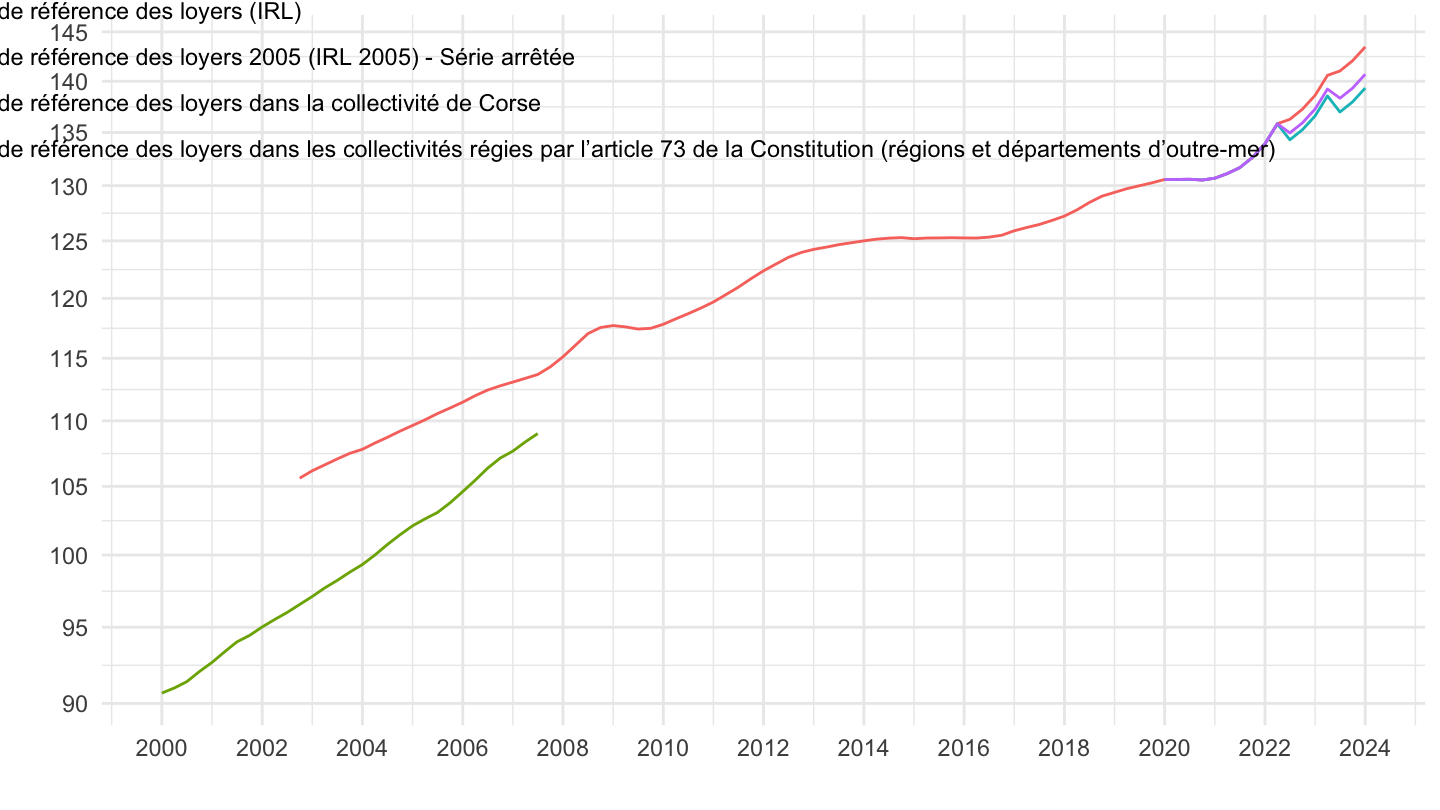

Variation annuelle

Tous

Code

IRL %>%
  filter(NATURE == "VARIATIONS_A") %>%
  quarter_to_date %>%
  ggplot(.) + theme_minimal() + ylab("") + xlab("") +
  geom_line(aes(x = date, y = OBS_VALUE/100, color = TITLE_FR)) +
  theme(legend.title = element_blank(),
        legend.position = c(0.5, 0.92)) +
  
  scale_x_date(breaks = seq(1950, 2100, 2) %>% paste0("-01-01") %>% as.Date,
               labels = date_format("%Y")) +
  scale_y_continuous(breaks = 0.01*seq(-200, 200, .5),
                     labels = percent_format(acc = .1),
                     limits = 0.01*c(-0.2, 4))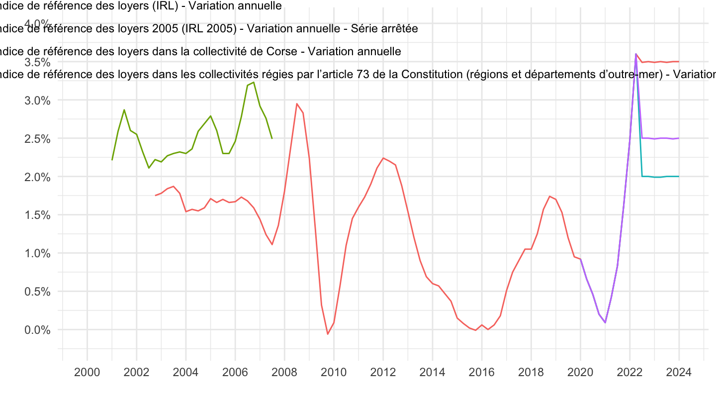

2008-

Code

table1 <- IRL %>%
  filter(NATURE == "VARIATIONS_A") %>%
  quarter_to_date %>%
  filter(date >= as.Date("2008-01-01")) %>%
  select(date, OBS_VALUE, IDBANK, TITLE_FR)

table1 %>%
  ggplot(.) + theme_minimal() + ylab("") + xlab("") +
  geom_line(aes(x = date, y = OBS_VALUE/100, color = TITLE_FR)) +
  theme(legend.title = element_blank(),
        legend.position = c(0.5, 0.92)) +
  
  scale_x_date(breaks = seq(1950, 2100, 2) %>% paste0("-01-01") %>% as.Date,
               labels = date_format("%Y")) +
  scale_y_continuous(breaks = 0.01*seq(-200, 200, .5),
                     labels = percent_format(acc = .1),
                     limits = 0.01*c(-0.2, 4))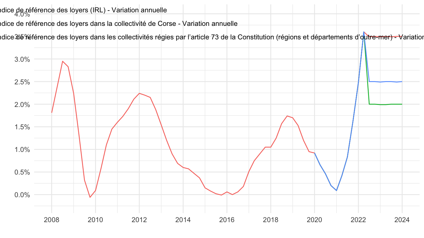

Table

Code

table1 %>%
  print_table_conditional()

Répliquer IRL à partir de l’Ensemble hors loyer hors tabac

Répliquer l’IRL à partir de l’ensemble hors loyer hors tabac.
Données IRL fournies ici: https://www.insee.fr/fr/statistiques/serie/001515334.
Peuvent être calculées juste à partir de l’IPC hors loyers, hors tabac: https://www.insee.fr/fr/statistiques/serie/001763862.

Prévisions INSEE

Estimation

Code

i_g("bib/insee/PdC_09-05-22/table5.png")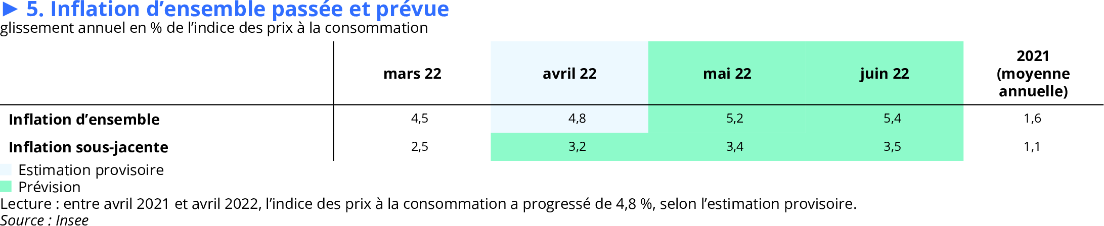

IRL Juillet

Code

`IPC-2015` %>%
  filter(PRIX_CONSO %in% c("4600"),
         COICOP2016 %in% c("00", "SO"),
         MENAGES_IPC == "ENSEMBLE",
         NATURE == "INDICE",
         REF_AREA == "FE",
         FREQ == "M") %>%
  select(TIME_PERIOD, OBS_VALUE) %>%
  arrange(desc(TIME_PERIOD))

# # A tibble: 0 × 2
# # ℹ 2 variables: TIME_PERIOD <chr>, OBS_VALUE <dbl>

En savoir plus

Liens

INSEE - La méthodologie de l’IRL. pdf
Dernier IRL. html
INSEE - méthodologie IRL base 1998. pdf
Indice de référence des loyers (IRL). html
Dernier indice IRL connu. html
Tableau sur le site de l’INSEE. html

Code

i_g("bib/insee/IR95_IRL_1T22/pour-en-savoir-plus.png")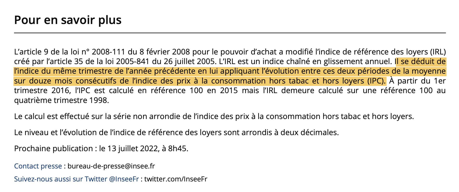

En savoir plus

L’article 9 de la loi no 2008-111 du 8 février 2008 pour le pouvoir d’achat a modifié l’indice de référence des loyers (IRL) créé par l’article 35 de la loi no 2005-841 du 26 juillet 2005. L’IRL est un indice chaîné en glissement annuel. Il se déduit de l’indice du même trimestre de l’année précédente en lui appliquant l’évolution entre ces deux périodes de la moyenne sur douze mois consécutifs de l’indice des prix à la consommation hors tabac et hors loyers (IPC). À partir du 1er trimestre 2016, l’IPC est calculé en référence 100 en 2015 mais l’IRL demeure calculé sur une référence 100 au quatrième trimestre 1998.

Le calcul est effectué sur la série non arrondie de l’indice des prix à la consommation hors tabac et hors loyers.

Le niveau et l’évolution de l’indice de référence des loyers sont arrondis à deux décimales.

Pour la fixation des indices de référence des loyers entre le troisième trimestre de l’année 2022 et le premier trimestre de l’année 2024, l’article 12 de la loi no 2022-1158 du 16 août 2022 portant mesures d’urgence pour la protection du pouvoir d’achat, modifié par l’article 2 de la loi no 2023-568 du 7 juillet 2023, dispose que « la variation en glissement annuel de l’indice de référence des loyers ne peut excéder 3,5 %. ».

L’article dispose également que cette variation ne peut excéder 2,5 % pour les départements et régions d’Outre-mer.

Enfin, l’arrêté no R20-2022-10-11-00012 modifié dispose que la variation en glissement annuel de l’indice de référence des loyers dans la collectivité de Corse ne peut excéder 2,0 % pour la fixation des indices de référence des loyers entre le troisième trimestre de l’année 2022 et le premier trimestre de l’année 2024.