| LAST_COMPILE |
|---|
| 2026-03-24 |
Inflation, consumer prices (annual %)
Data - WDI
Info
LAST_COMPILE
Last
Code
FP.CPI.TOTL.ZG %>%
  group_by(year) %>%
  summarise(Nobs = n()) %>%
  arrange(desc(year)) %>%
  head(1) %>%
print_table_conditional()| year | Nobs |
|---|---|
| 2024 | 219 |
Nobs - Javascript
Code
FP.CPI.TOTL.ZG %>%
  left_join(iso2c, by = "iso2c") %>%
  group_by(iso2c, Iso2c) %>%
  summarise(Nobs = n(),
            `Year 1` = first(year),
            `Inflation 1` = round(first(value), 2) %>% paste0(" %"),
            `Year 2` = last(year),
            `Inflation 2` = round(last(value), 2) %>% paste0(" %")) %>%
  arrange(-Nobs) %>%
  {if (is_html_output()) datatable(., filter = 'top', rownames = F) else .}
Periods of Low Inflation
Code
FP.CPI.TOTL.ZG %>%
  filter(value < 0) %>%
  arrange(value) %>%
  mutate(value = round(value, 2)) %>%
  left_join(iso2c, by = "iso2c") %>%
  select(iso2c, Iso2c, year, value) %>%
  {if (is_html_output()) datatable(., filter = 'top', rownames = F) else .}
France
All
Code
data %>%
  left_join(INDICATOR) %>%
  year_to_date() %>%
  filter(iso2c == "FR") %>%
  ggplot(.) + theme_minimal() + xlab("") + ylab("Inflation (%)") +
  geom_line(aes(x = date, y = value/100, color = Indicator)) +

  theme(legend.title = element_blank(),
        legend.position = c(0.65, 0.85)) +
  scale_x_date(breaks = seq(1900, 2100, 5) %>% paste0("-01-01") %>% as.Date,
               labels = date_format("%Y")) +
  scale_y_continuous(breaks = 0.01*seq(-100, 10000, 2),
                     labels = percent_format(a = 1)) +
  geom_hline(yintercept = 0, linetype = "dashed", color = "black")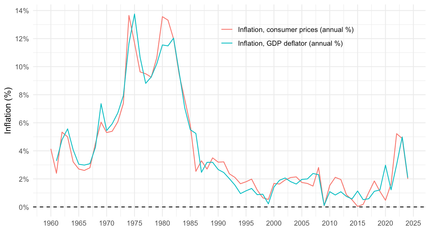
1993-
Code
data %>%
  left_join(INDICATOR) %>%
  year_to_date() %>%
  filter(iso2c == "FR",
         date >= as.Date("1993-01-01")) %>%
  ggplot(.) + theme_minimal() + xlab("") + ylab("Inflation (%)") +
  geom_line(aes(x = date, y = value/100, color = Indicator)) +

  theme(legend.title = element_blank(),
        legend.position = c(0.55, 0.85)) +
  scale_x_date(breaks = seq(1900, 2100, 2) %>% paste0("-01-01") %>% as.Date,
               labels = date_format("%Y")) +
  scale_y_continuous(breaks = 0.01*seq(-100, 10000, 1),
                     labels = percent_format(a = 1)) +
  geom_hline(yintercept = 0, linetype = "dashed", color = "black")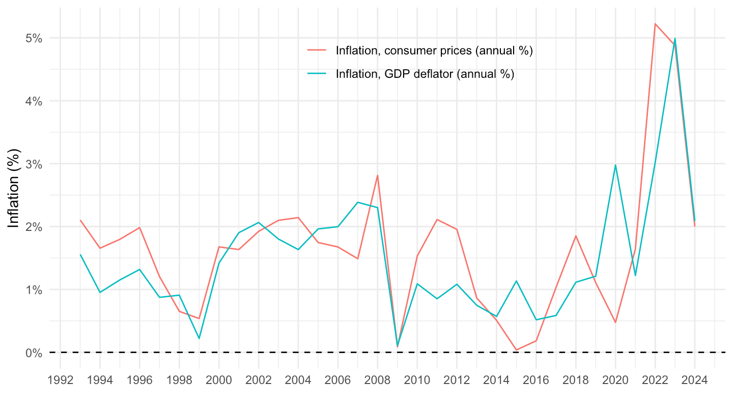
2017-
Code
data %>%
  left_join(INDICATOR) %>%
  year_to_date() %>%
  filter(iso2c == "FR",
         date >= as.Date("2017-01-01")) %>%
  mutate(value = value/100) %>%
  ggplot(.) + theme_minimal() + xlab("") + ylab("Inflation (%)") +
  geom_line(aes(x = date, y = value, color = Indicator)) +

  theme(legend.title = element_blank(),
        legend.position = c(0.3, 0.85)) +
  scale_x_date(breaks = seq(1900, 2100, 1) %>% paste0("-01-01") %>% as.Date,
               labels = date_format("%Y")) +
  scale_y_continuous(breaks = 0.01*seq(-100, 10000, 1),
                     labels = percent_format(a = 1)) +
  geom_hline(yintercept = 0, linetype = "dashed", color = "black") +
  geom_text_repel(aes(x = date, y = value, label = percent(value, acc = 0.1), color = Indicator))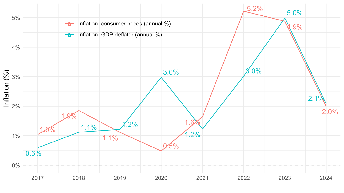
Israel
All
Code
data %>%
  left_join(INDICATOR) %>%
  year_to_date() %>%
  filter(iso2c == "IS") %>%
  ggplot(.) + theme_minimal() + xlab("") + ylab("Inflation (%)") +
  geom_line(aes(x = date, y = value/100, color = Indicator)) +

  theme(legend.title = element_blank(),
        legend.position = c(0.65, 0.85)) +
  scale_x_date(breaks = seq(1900, 2100, 5) %>% paste0("-01-01") %>% as.Date,
               labels = date_format("%Y")) +
  scale_y_continuous(breaks = 0.01*seq(-100, 10000, 5),
                     labels = percent_format(a = 1)) +
  geom_hline(yintercept = 0, linetype = "dashed", color = "black")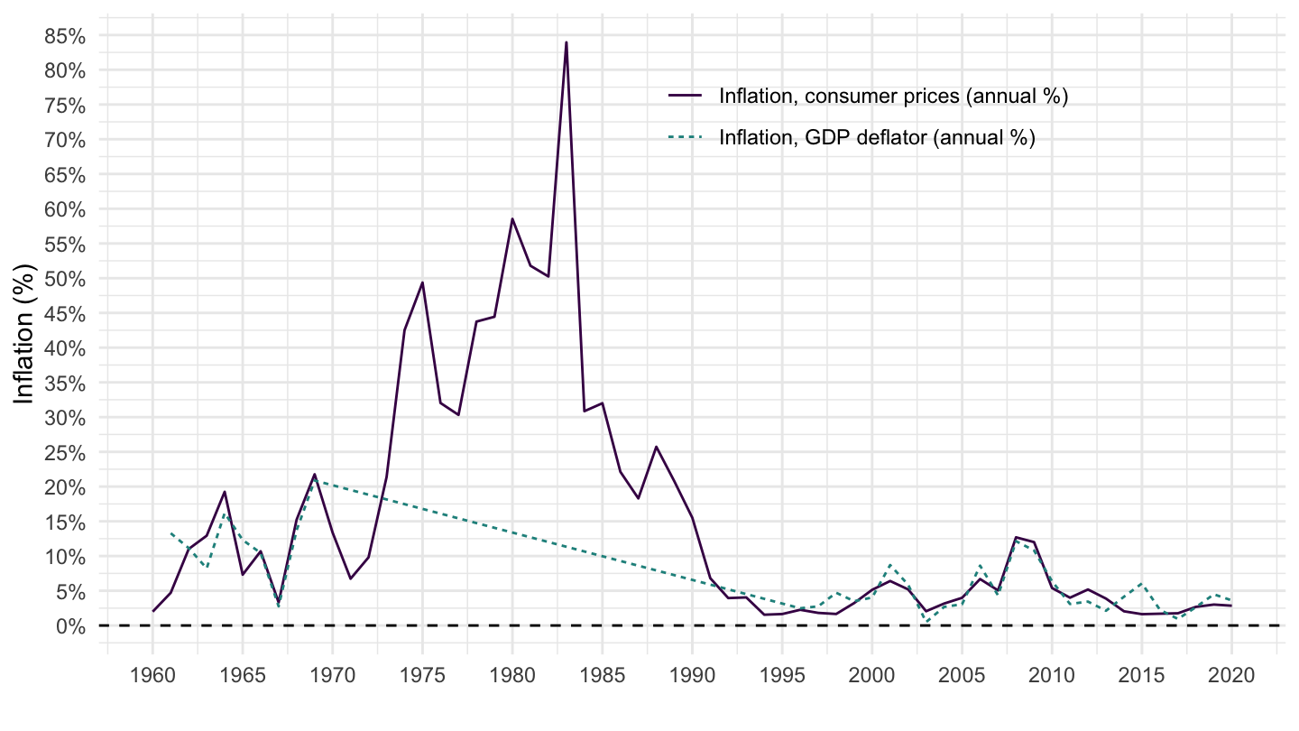
1993-
Code
data %>%
  left_join(INDICATOR) %>%
  year_to_date() %>%
  filter(iso2c == "IS",
         date >= as.Date("1993-01-01")) %>%
  ggplot(.) + theme_minimal() + xlab("") + ylab("Inflation (%)") +
  geom_line(aes(x = date, y = value/100, color = Indicator)) +

  theme(legend.title = element_blank(),
        legend.position = c(0.25, 0.85)) +
  scale_x_date(breaks = seq(1900, 2100, 2) %>% paste0("-01-01") %>% as.Date,
               labels = date_format("%Y")) +
  scale_y_continuous(breaks = 0.01*seq(-100, 10000, 2),
                     labels = percent_format(a = 1)) +
  geom_hline(yintercept = 0, linetype = "dashed", color = "black")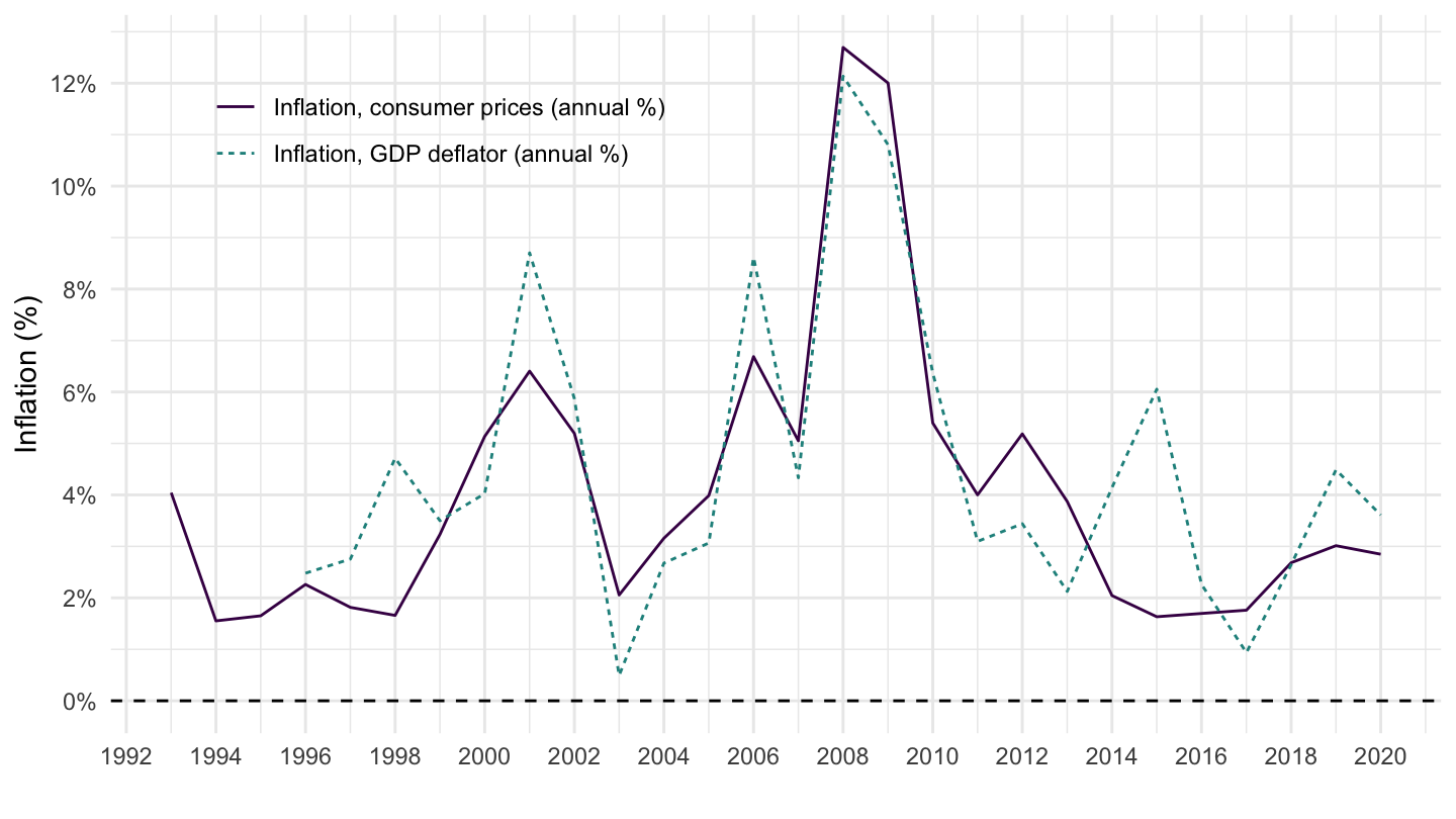
1990-2000
Code
FP.CPI.TOTL.ZG %>%
  year_to_date() %>%
  filter(iso2c == "IS",
         date >= as.Date("1990-01-01"),
         date <= as.Date("2000-01-01")) %>%
  ggplot(.) + geom_line() + theme_minimal() +
  aes(x = date, y = value/100) + xlab("") + ylab("Inflation (%)") +
  scale_x_date(breaks = seq(1900, 2100, 1) %>% paste0("-01-01") %>% as.Date,
               labels = date_format("%Y")) +
  scale_y_continuous(breaks = 0.01*seq(-100, 10000, 5),
                     labels = percent_format(a = 1)) +
  geom_hline(yintercept = 0, linetype = "dashed", color = "grey")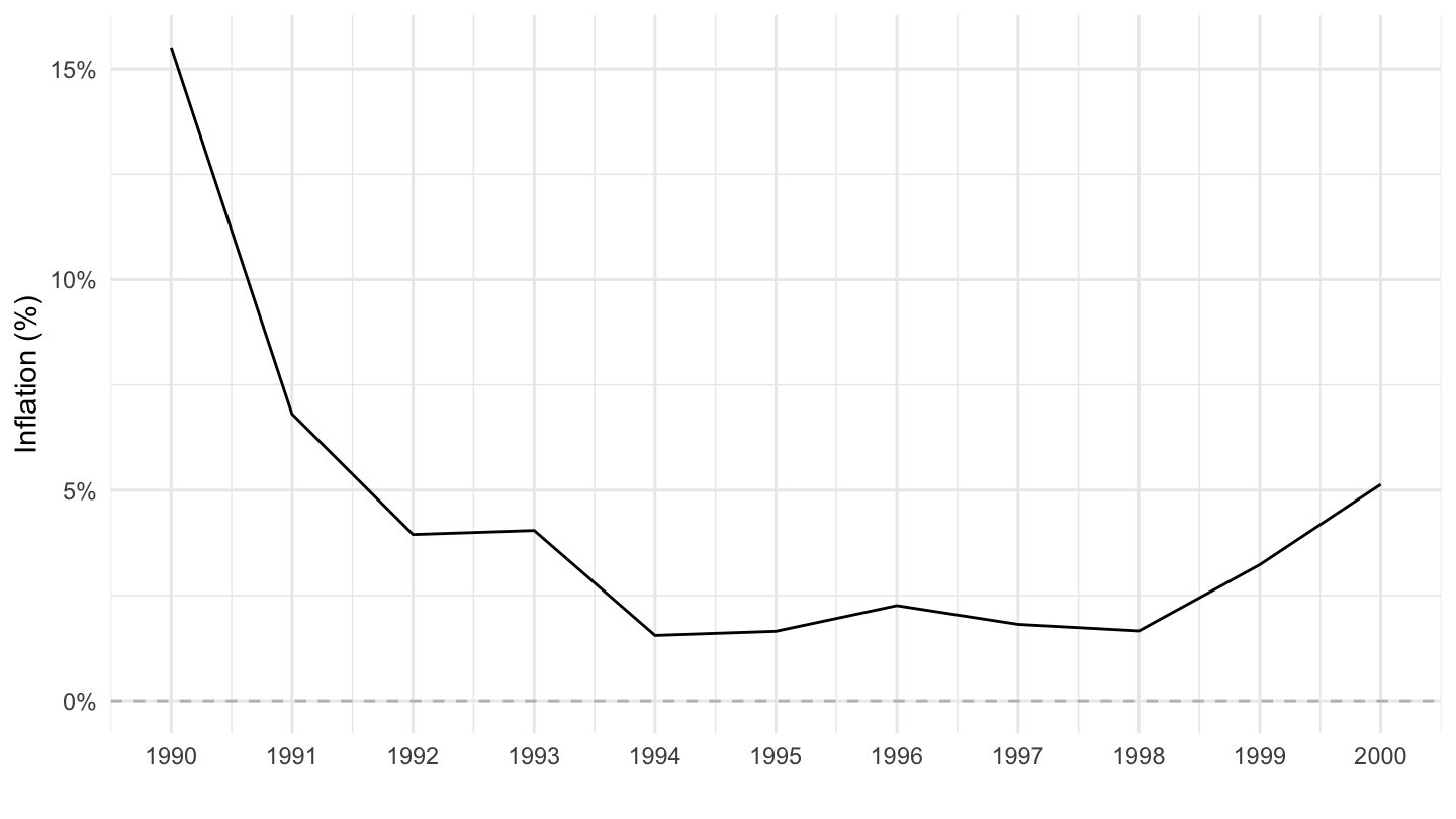
Hungary
All
Code
data %>%
  left_join(INDICATOR) %>%
  year_to_date() %>%
  filter(iso2c == "HU") %>%
  ggplot(.) + theme_minimal() + xlab("") + ylab("Inflation (%)") +
  geom_line(aes(x = date, y = value/100, color = Indicator)) +

  theme(legend.title = element_blank(),
        legend.position = c(0.65, 0.85)) +
  scale_x_date(breaks = seq(1900, 2100, 5) %>% paste0("-01-01") %>% as.Date,
               labels = date_format("%Y")) +
  scale_y_continuous(breaks = 0.01*seq(-100, 10000, 5),
                     labels = percent_format(a = 1)) +
  geom_hline(yintercept = 0, linetype = "dashed", color = "black")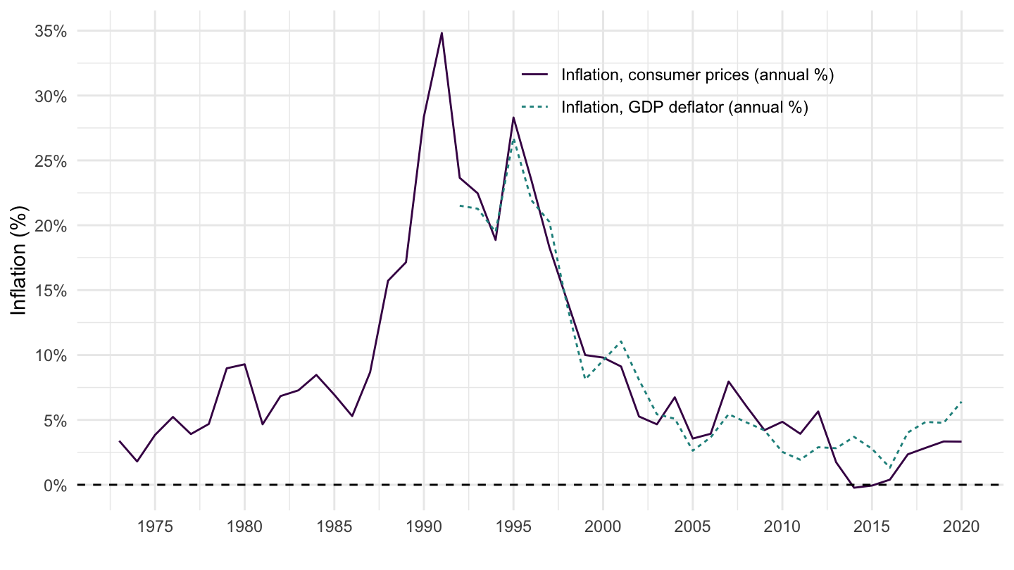
1993-
Code
data %>%
  left_join(INDICATOR) %>%
  year_to_date() %>%
  filter(iso2c == "HU",
         date >= as.Date("1993-01-01")) %>%
  ggplot(.) + theme_minimal() + xlab("") + ylab("Inflation (%)") +
  geom_line(aes(x = date, y = value/100, color = Indicator)) +

  theme(legend.title = element_blank(),
        legend.position = c(0.55, 0.85)) +
  scale_x_date(breaks = seq(1900, 2100, 2) %>% paste0("-01-01") %>% as.Date,
               labels = date_format("%Y")) +
  scale_y_continuous(breaks = 0.01*seq(-100, 10000, 2),
                     labels = percent_format(a = 1)) +
  geom_hline(yintercept = 0, linetype = "dashed", color = "black")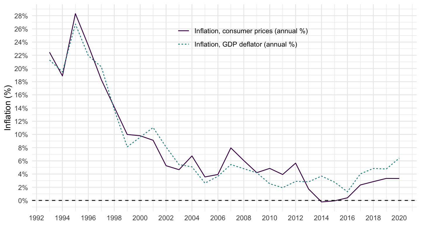
South Korea
All
Code
data %>%
  left_join(INDICATOR) %>%
  year_to_date() %>%
  filter(iso2c == "KR") %>%
  ggplot(.) + theme_minimal() + xlab("") + ylab("Inflation (%)") +
  geom_line(aes(x = date, y = value/100, color = Indicator)) +

  theme(legend.title = element_blank(),
        legend.position = c(0.65, 0.85)) +
  scale_x_date(breaks = seq(1900, 2100, 5) %>% paste0("-01-01") %>% as.Date,
               labels = date_format("%Y")) +
  scale_y_continuous(breaks = 0.01*seq(-100, 10000, 5),
                     labels = percent_format(a = 1)) +
  geom_hline(yintercept = 0, linetype = "dashed", color = "black")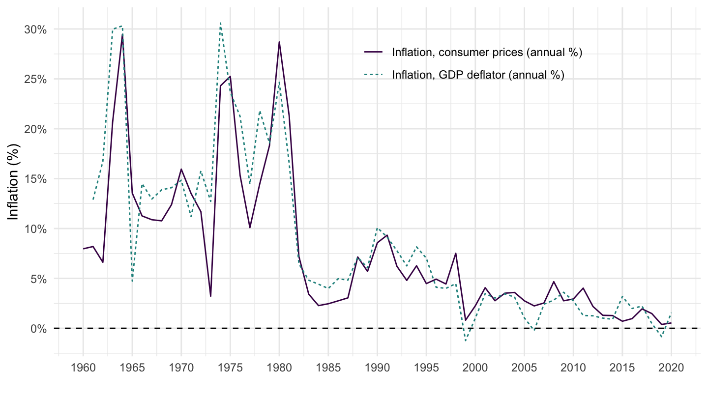
1993-
Code
data %>%
  left_join(INDICATOR) %>%
  year_to_date() %>%
  filter(iso2c == "KR",
         date >= as.Date("1993-01-01")) %>%
  ggplot(.) + theme_minimal() + xlab("") + ylab("Inflation (%)") +
  geom_line(aes(x = date, y = value/100, color = Indicator)) +

  theme(legend.title = element_blank(),
        legend.position = c(0.55, 0.85)) +
  scale_x_date(breaks = seq(1900, 2100, 2) %>% paste0("-01-01") %>% as.Date,
               labels = date_format("%Y")) +
  scale_y_continuous(breaks = 0.01*seq(-100, 10000, 2),
                     labels = percent_format(a = 1)) +
  geom_hline(yintercept = 0, linetype = "dashed", color = "black")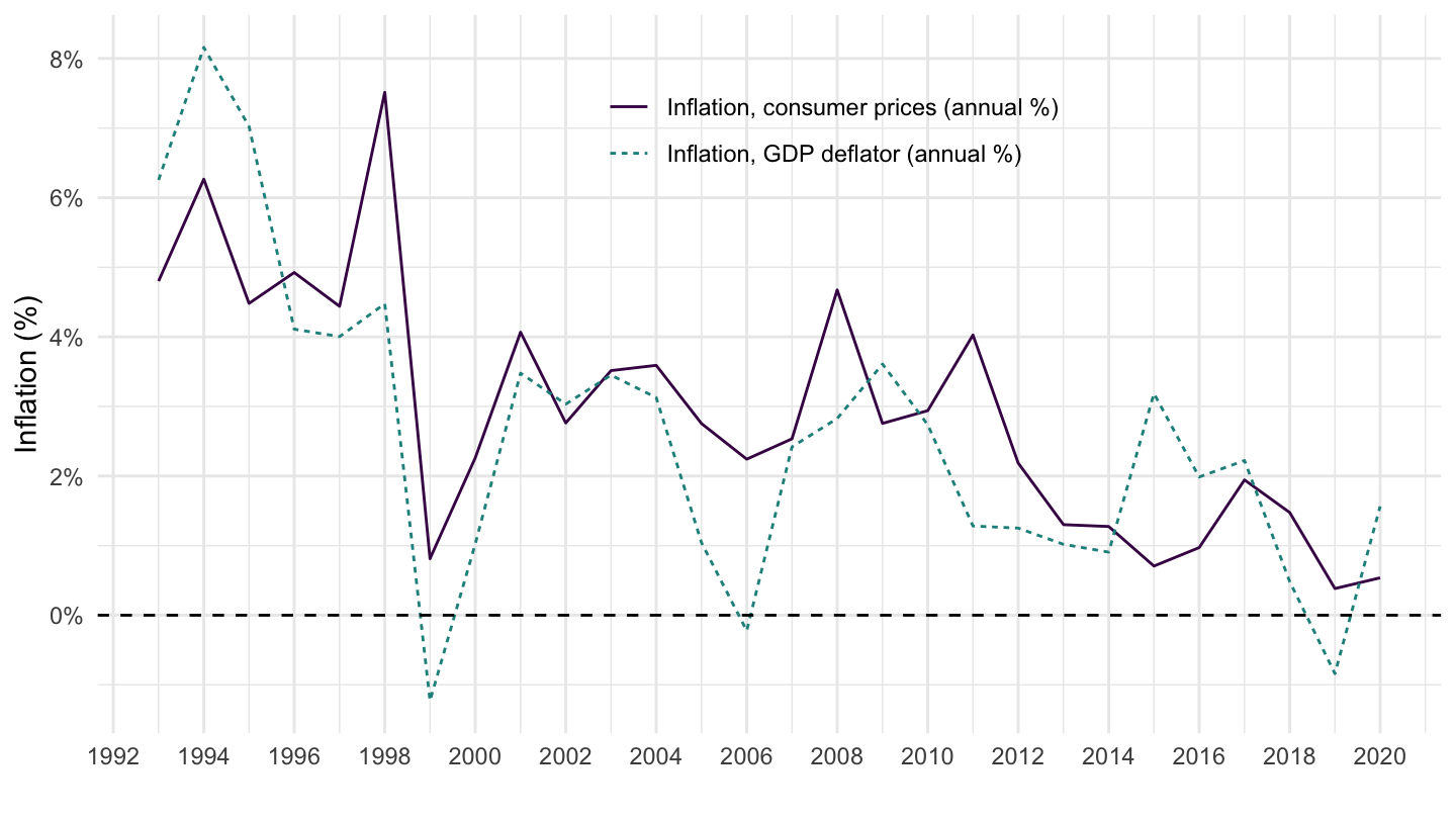
Mexico
All
Code
FP.CPI.TOTL.ZG %>%
  year_to_date() %>%
  filter(iso2c == "MX") %>%
  ggplot(.) + geom_line() + theme_minimal() +
  aes(x = date, y = value/100) + xlab("") + ylab("Inflation (%)") +
  scale_x_date(breaks = seq(1900, 2100, 10) %>% paste0("-01-01") %>% as.Date,
               labels = date_format("%Y")) +
  scale_y_continuous(breaks = 0.01*seq(-100, 10000, 10),
                     labels = percent_format(a = 1)) +
  geom_hline(yintercept = 0, linetype = "dashed", color = "grey")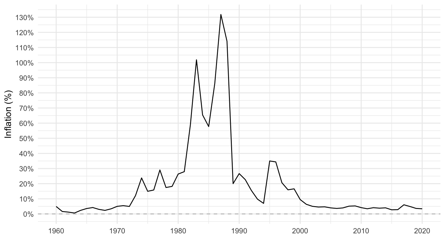
1990-2000
Code
FP.CPI.TOTL.ZG %>%
  year_to_date() %>%
  filter(iso2c == "MX",
         date >= as.Date("1990-01-01"),
         date <= as.Date("2000-01-01")) %>%
  ggplot(.) + geom_line() + theme_minimal() +
  aes(x = date, y = value/100) + xlab("") + ylab("Inflation (%)") +
  scale_x_date(breaks = seq(1900, 2100, 1) %>% paste0("-01-01") %>% as.Date,
               labels = date_format("%Y")) +
  scale_y_continuous(breaks = 0.01*seq(-100, 10000, 5),
                     labels = percent_format(a = 1)) +
  geom_hline(yintercept = 0, linetype = "dashed", color = "grey")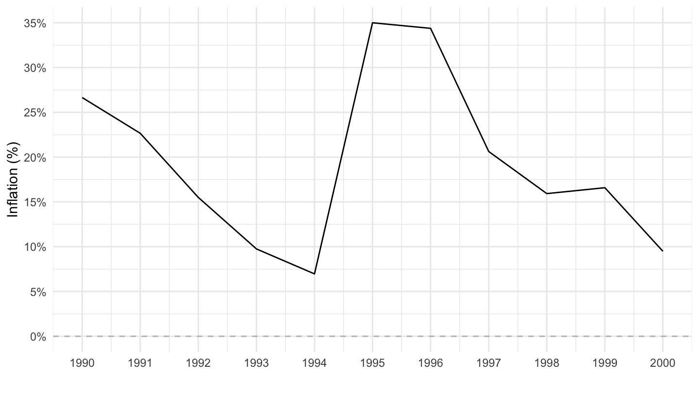
Sri Lanka, Nigeria, Pakistan
All
Code
FP.CPI.TOTL.ZG %>%
  filter(iso2c %in% c("LK", "NG", "PK")) %>%
  left_join(iso2c, by = "iso2c") %>%
  year_to_date() %>%
  left_join(colors, by = c("Iso2c" = "country")) %>%
  mutate(value = value/100) %>%
  ggplot(.) + geom_line(aes(x = date, y = value, color = color)) +
  xlab("") + ylab("Inflation, consumer prices") +
  theme_minimal() + scale_color_identity() + add_3flags +
  scale_x_date(breaks = seq(1900, 2100, 5) %>% paste0("-01-01") %>% as.Date,
               labels = date_format("%Y")) +
  scale_y_continuous(breaks = 0.01*seq(-100, 10000, 2),
                     labels = percent_format(a = 1)) +
  geom_hline(yintercept = 0, linetype = "dashed", color = "grey")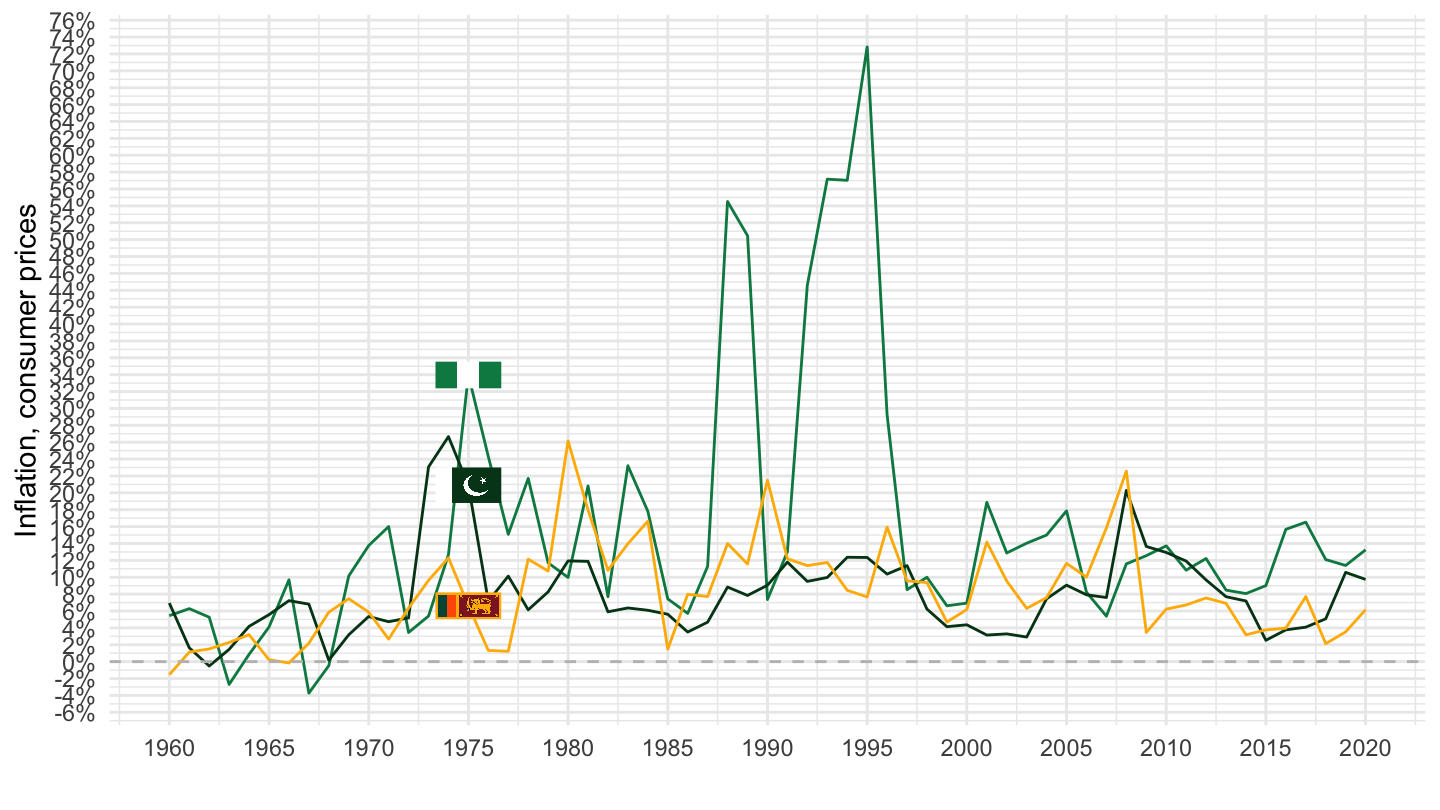
2000-
Code
FP.CPI.TOTL.ZG %>%
  filter(iso2c %in% c("LK", "NG", "PK")) %>%
  left_join(iso2c, by = "iso2c") %>%
  year_to_date() %>%
  filter(date >+ as.Date("2000-01-01")) %>%
  left_join(colors, by = c("Iso2c" = "country")) %>%
  mutate(value = value/100) %>%
  ggplot(.) + geom_line(aes(x = date, y = value, color = color)) +
  xlab("") + ylab("Inflation, consumer prices") +
  theme_minimal() + scale_color_identity() + add_3flags +
  scale_x_date(breaks = seq(1900, 2100, 2) %>% paste0("-01-01") %>% as.Date,
               labels = date_format("%Y")) +
  scale_y_continuous(breaks = 0.01*seq(-100, 10000, 2),
                     labels = percent_format(a = 1)) +
  geom_hline(yintercept = 0, linetype = "dashed", color = "grey")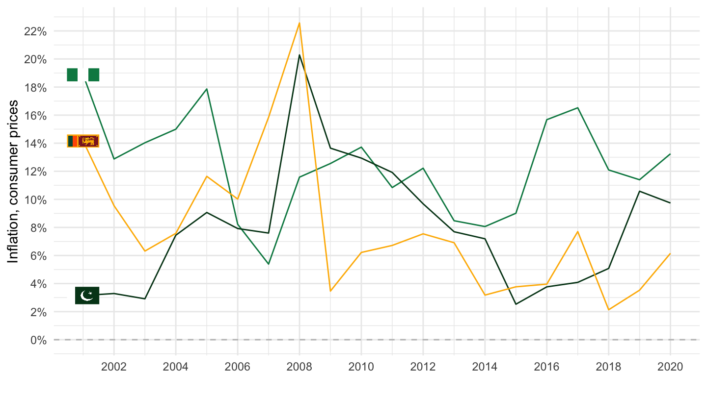
France, Italy, Germany
All
Code
FP.CPI.TOTL.ZG %>%
  filter(iso2c %in% c("FR", "DE", "IT")) %>%
  left_join(iso2c, by = "iso2c") %>%
  year_to_date() %>%
  left_join(colors, by = c("Iso2c" = "country")) %>%
  mutate(value = value/100) %>%
  ggplot(.) + geom_line(aes(x = date, y = value, color = color)) +
  xlab("") + ylab("Inflation, consumer prices") +
  theme_minimal() + scale_color_identity() + add_3flags +
  scale_x_date(breaks = seq(1900, 2100, 5) %>% paste0("-01-01") %>% as.Date,
               labels = date_format("%Y")) +
  scale_y_continuous(breaks = 0.01*seq(-100, 10000, 2),
                     labels = percent_format(a = 1)) +
  geom_hline(yintercept = 0, linetype = "dashed", color = "grey")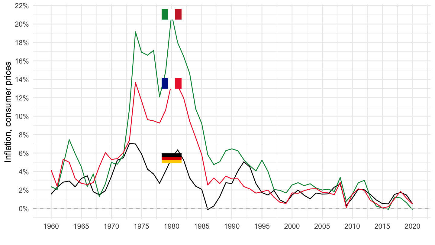
2017-
Code
FP.CPI.TOTL.ZG %>%
  filter(iso2c %in% c("FR", "DE", "IT")) %>%
  left_join(iso2c, by = "iso2c") %>%
  year_to_date() %>%
  left_join(colors, by = c("Iso2c" = "country")) %>%
  mutate(value = value/100) %>%
  filter(date >= as.Date("2017-01-01")) %>%
  ggplot(.) + geom_line(aes(x = date, y = value, color = color)) +
  xlab("") + ylab("Inflation, consumer prices") +
  theme_minimal() + scale_color_identity() + add_3flags +
  scale_x_date(breaks = seq(1900, 2100, 1) %>% paste0("-01-01") %>% as.Date,
               labels = date_format("%Y")) +
  scale_y_continuous(breaks = 0.01*seq(-100, 10000, 1),
                     labels = percent_format(a = 1)) +
  geom_hline(yintercept = 0, linetype = "dashed", color = "grey")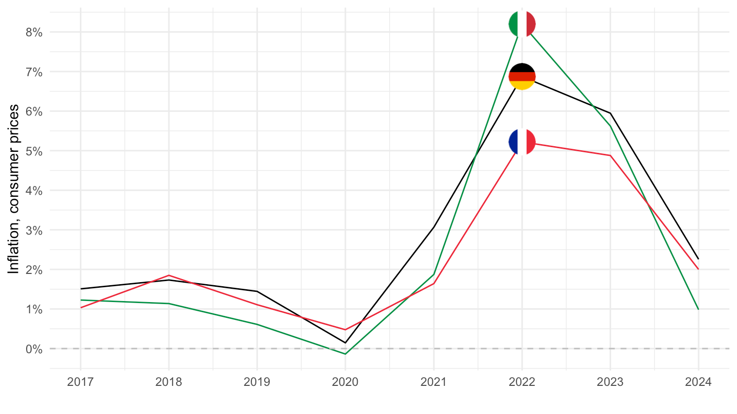
France, Italy, Germany, Spain, Portugal
Code
FP.CPI.TOTL.ZG %>%
  filter(iso2c %in% c("FR", "DE", "IT", "ES", "PT")) %>%
  left_join(iso2c, by = "iso2c") %>%
  year_to_date() %>%
  left_join(colors, by = c("Iso2c" = "country")) %>%
  mutate(value = value/100) %>%
  ggplot(.) + geom_line(aes(x = date, y = value, color = color)) +
  xlab("") + ylab("Inflation, consumer prices") +
  theme_minimal() + scale_color_identity() + add_5flags +
  scale_x_date(breaks = seq(1900, 2025, 5) %>% paste0("-01-01") %>% as.Date,
               labels = date_format("%Y")) +
  scale_y_continuous(breaks = 0.01*seq(-100, 10000, 2),
                     labels = percent_format(a = 1)) +
  geom_hline(yintercept = 0, linetype = "dashed", color = "grey")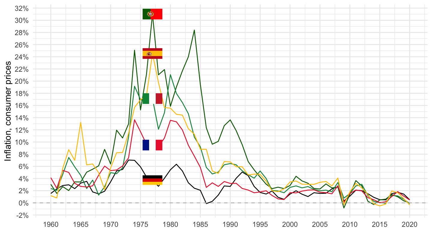
Denmark, Netherlands, Sweden
Code
FP.CPI.TOTL.ZG %>%
  filter(iso2c %in% c("DK", "SE", "NL")) %>%
  left_join(iso2c, by = "iso2c") %>%
  year_to_date() %>%
  left_join(colors, by = c("Iso2c" = "country")) %>%
  mutate(value = value/100) %>%
  ggplot(.) + geom_line(aes(x = date, y = value, color = color)) +
  xlab("") + ylab("Inflation, consumer prices") +
  theme_minimal() + scale_color_identity() + add_3flags +
  scale_x_date(breaks = seq(1900, 2100, 5) %>% paste0("-01-01") %>% as.Date,
               labels = date_format("%Y")) +
  scale_y_continuous(breaks = 0.01*seq(-100, 10000, 2),
                     labels = percent_format(a = 1)) +
  geom_hline(yintercept = 0, linetype = "dashed", color = "grey")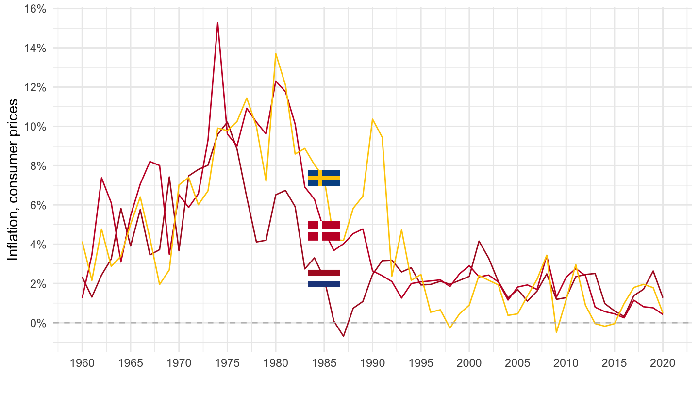
United States, United Kingdom, Japan
All
Code
FP.CPI.TOTL.ZG %>%
  filter(iso2c %in% c("JP", "US", "GB")) %>%
  left_join(iso2c, by = "iso2c") %>%
  year_to_date() %>%
  left_join(colors, by = c("Iso2c" = "country")) %>%
  mutate(value = value/100) %>%
  ggplot(.) + geom_line(aes(x = date, y = value, color = color)) +
  xlab("") + ylab("Inflation, consumer prices") +
  theme_minimal() + scale_color_identity() + add_3flags +
  scale_x_date(breaks = seq(1900, 2100, 5) %>% paste0("-01-01") %>% as.Date,
               labels = date_format("%Y")) +
  scale_y_continuous(breaks = 0.01*seq(-100, 10000, 2),
                     labels = percent_format(a = 1)) +
  geom_hline(yintercept = 0, linetype = "dashed", color = "grey")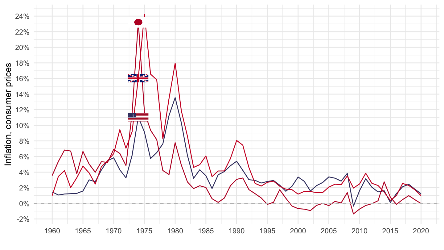
2017-
Code
FP.CPI.TOTL.ZG %>%
  filter(iso2c %in% c("JP", "US", "GB")) %>%
  left_join(iso2c, by = "iso2c") %>%
  year_to_date() %>%
  left_join(colors, by = c("Iso2c" = "country")) %>%
  mutate(value = value/100) %>%
  filter(date >= as.Date("2017-01-01")) %>%
  ggplot(.) + geom_line(aes(x = date, y = value, color = color)) +
  xlab("") + ylab("Inflation, consumer prices") +
  theme_minimal() + scale_color_identity() + add_3flags +
  scale_x_date(breaks = seq(1900, 2100, 1) %>% paste0("-01-01") %>% as.Date,
               labels = date_format("%Y")) +
  scale_y_continuous(breaks = 0.01*seq(-100, 10000, 1),
                     labels = percent_format(a = 1)) +
  geom_hline(yintercept = 0, linetype = "dashed", color = "grey")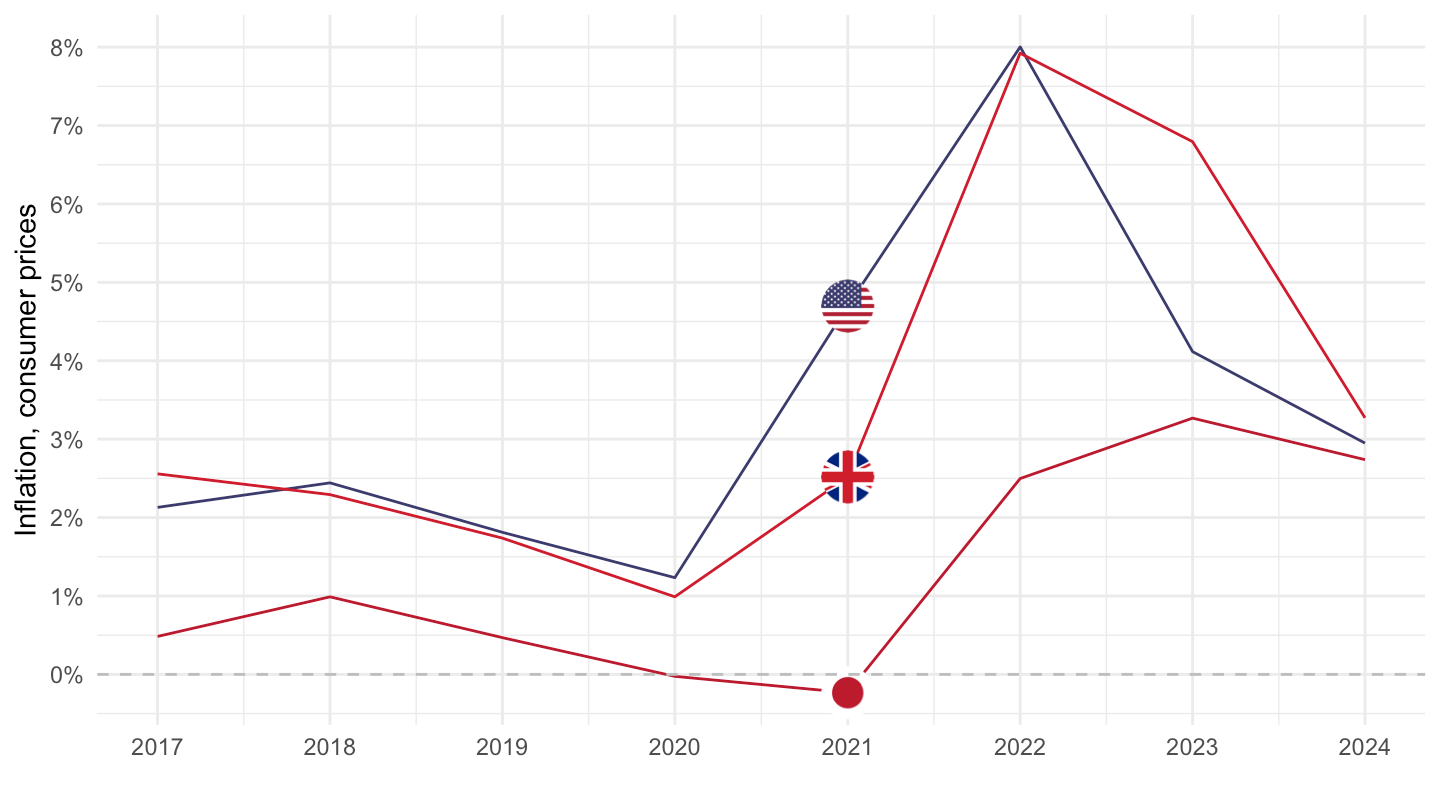
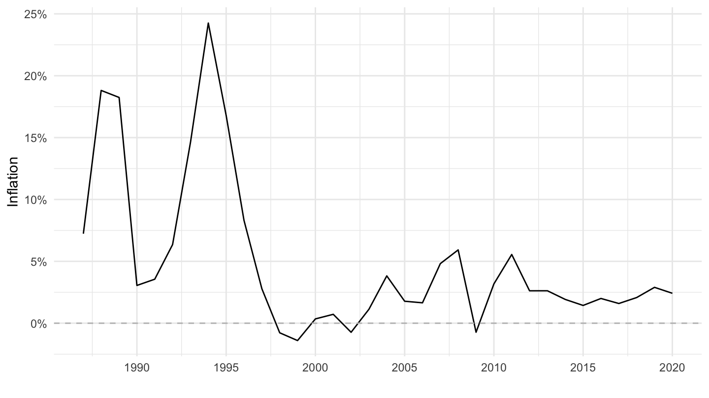
China
Code
FP.CPI.TOTL.ZG %>%
  filter(iso2c == "CN") %>%
  year_to_date() %>%
  ggplot(.) + geom_line() + theme_minimal() +
  aes(x = date, y = value/100) + xlab("") + ylab("Inflation") +
  scale_x_date(breaks = seq(1900, 2100, 5) %>% paste0("-01-01") %>% as.Date,
               labels = date_format("%Y")) +
  scale_y_continuous(breaks = 0.01*seq(-100, 10000, 5),
                     labels = percent_format(a = 1)) +
  geom_hline(yintercept = 0, linetype = "dashed", color = "grey")