
Last observation: déc. 2025 (N = 424) · 2025 (N = 840)
First observation: 1996 (N = 714) · janv. 1996 (N = 357)
Last data update: 09 oct. 2026, 22:47
Last compile: 10 oct. 2026, 01:15
Moyenne annuelle: l’évolution en moyenne annuelle compare les prix d’une année donnée à ceux de l’année précédente.
Glissement annuel: l’évolution en glissement annuel compare les prix d’un seul mois d’une année donnée à ceux du même mois de l’année précédente.
`IPCH-2015` |>
  filter(NATURE == "GLISSEMENT_ANNUEL") |>
  month_to_date() |>
  ggplot() + ylab("Glissement annuel (%)") + xlab("") + theme_minimal() +
  geom_line(aes(x = date, y = OBS_VALUE/100)) +
  theme(legend.position = c(0.3, 0.8),
        legend.title = element_blank()) +
  scale_x_date(breaks = seq(1920, 2100, 2) |> paste0("-01-01") |> as.Date(),
               labels = date_format("%Y")) +
  scale_y_continuous(breaks = 0.01*seq(-10, 10, 1),
                     labels = percent_format())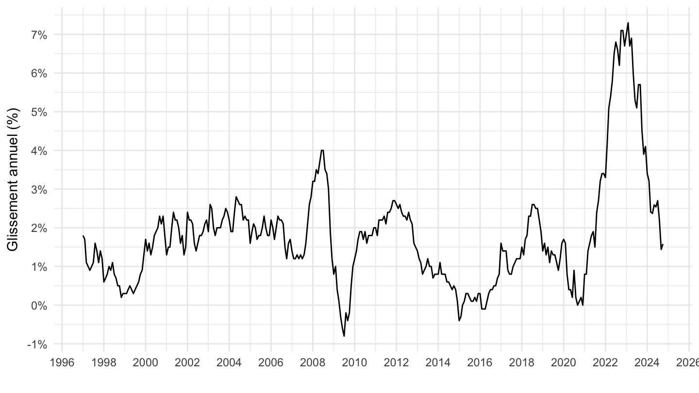
`IPCH-IPC-2015-ensemble` |>
  group_by(INDICATEUR) |>
  summarise(First_value = first(OBS_VALUE),
            First_date = first(date),
            Last_value = last(OBS_VALUE),
            Last_date = last(date)) |>
print_table_conditional()| INDICATEUR | First_value | First_date | Last_value | Last_date |
|---|---|---|---|---|
| IPC | 100 | 1996-01-01 | 159.1418 | 2025-12-01 |
| IPCH | 100 | 1996-01-01 | 167.9217 | 2025-12-01 |
`IPCH-2015` |>
  bind_rows(`IPC-2015`) |>
  filter(COICOP2016 %in% c("00"),
         NATURE == "INDICE",
         REF_AREA == "FE",
         FREQ == "A",
         is.na(MENAGES_IPC) | MENAGES_IPC == "ENSEMBLE",
         is.na(PRIX_CONSO) | PRIX_CONSO == "SO") |>
  year_to_date() |>
  filter(date >= Sys.Date() - years(6)) |>

  group_by(INDICATEUR) |>
  arrange(date) |>
  mutate(OBS_VALUE = OBS_VALUE/lag(OBS_VALUE)-1) |>
  select(date, OBS_VALUE, INDICATEUR) |>
  na.omit() |>
  ggplot() + ylab("Inflation annuelle") + xlab("") + theme_minimal() +
  geom_line(aes(x = date, y = OBS_VALUE, color = INDICATEUR)) +
  #
  theme(legend.position = c(0.6, 0.2),
        legend.title = element_blank()) +
  scale_x_date(breaks = seq(1920, 2100, 1) |> paste0("-01-01") |> as.Date(),
               labels = date_format("%Y")) +
  scale_y_continuous(breaks = 0.01*seq(-10, 10, 1),
                     labels = percent_format()) +
  geom_label(aes(x = date, y = OBS_VALUE, label = percent(OBS_VALUE, acc = 0.1), color = INDICATEUR),
                  fontface ="plain", size = 3)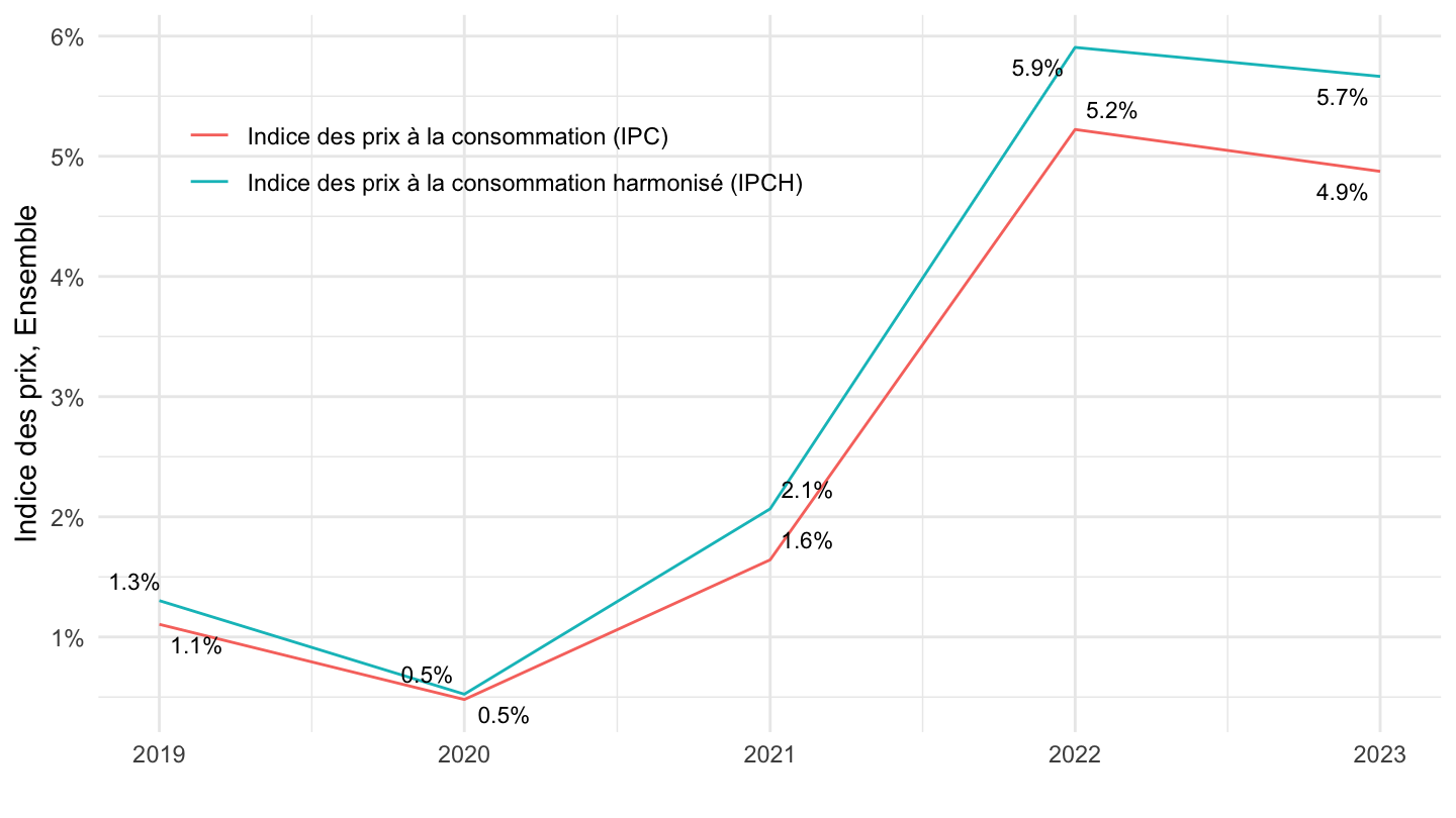
`IPCH-2015` |>
  bind_rows(`IPC-2015`) |>
  filter(COICOP2016 %in% c("00"),
         NATURE == "INDICE",
         REF_AREA == "FE",
         FREQ == "A",
         is.na(MENAGES_IPC) | MENAGES_IPC == "ENSEMBLE",
         is.na(PRIX_CONSO) | PRIX_CONSO == "SO") |>
  year_to_date() |>
  filter(date >= Sys.Date() - years(12)) |>

  group_by(INDICATEUR) |>
  arrange(date) |>
  mutate(OBS_VALUE = OBS_VALUE/lag(OBS_VALUE)-1) |>
  select(date, OBS_VALUE, INDICATEUR) |>
  na.omit() |>
  ggplot() + ylab("Indice des prix, Ensemble") + xlab("") + theme_minimal() +
  geom_line(aes(x = date, y = OBS_VALUE, color = INDICATEUR)) +
  #
  theme(legend.position = c(0.3, 0.8),
        legend.title = element_blank()) +
  scale_x_date(breaks = seq(1920, 2100, 1) |> paste0("-01-01") |> as.Date(),
               labels = date_format("%Y")) +
  scale_y_continuous(breaks = 0.01*seq(-10, 10, 1),
                     labels = percent_format()) +
  geom_text_repel(aes(x = date, y = OBS_VALUE, label = percent(OBS_VALUE, acc = 0.1), color = INDICATEUR),
                  fontface ="plain", size = 3)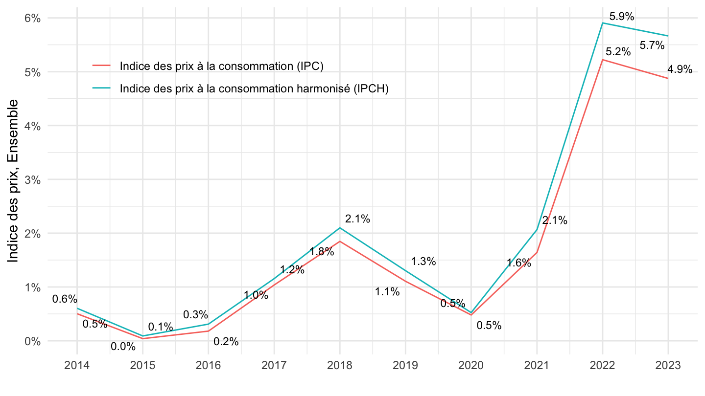
`IPCH-2015` |>
  bind_rows(`IPC-2015`) |>
  filter(COICOP2016 %in% c("00"),
         NATURE == "INDICE",
         REF_AREA == "FE",
         FREQ == "A",
         is.na(MENAGES_IPC) | MENAGES_IPC == "ENSEMBLE",
         is.na(PRIX_CONSO) | PRIX_CONSO == "SO") |>
  year_to_date() |>
  filter(date >= as.Date("2010-01-01"),
         date <= as.Date("2021-01-01")) |>

  group_by(INDICATEUR) |>
  arrange(date) |>
  mutate(OBS_VALUE = OBS_VALUE/lag(OBS_VALUE)-1) |>
  select(date, OBS_VALUE, INDICATEUR) |>
  na.omit() |>
  ggplot() + ylab("Indice des prix, Ensemble") + xlab("") + theme_minimal() +
  geom_line(aes(x = date, y = OBS_VALUE, color = INDICATEUR)) +
  #
  theme(legend.position = c(0.5, 0.9),
        legend.title = element_blank()) +
  scale_x_date(breaks = seq(1920, 2100, 1) |> paste0("-01-01") |> as.Date(),
               labels = date_format("%Y")) +
  scale_y_continuous(breaks = 0.01*seq(-10, 10, 1),
                     labels = percent_format()) +
  geom_text_repel(aes(x = date, y = OBS_VALUE, label = percent(OBS_VALUE, acc = 0.001), color = INDICATEUR),
                  fontface ="plain", size = 3, show.legend = F)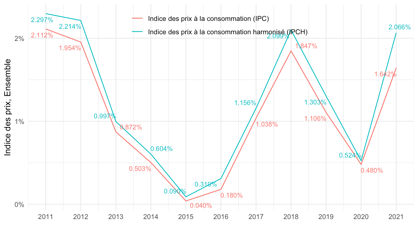
`IPCH-2015` |>
  bind_rows(`IPC-2015`) |>
  filter(COICOP2016 %in% c("00"),
         NATURE == "INDICE",
         REF_AREA == "FE",
         FREQ == "A",
         is.na(MENAGES_IPC) | MENAGES_IPC == "ENSEMBLE",
         is.na(PRIX_CONSO) | PRIX_CONSO == "SO") |>
  year_to_date() |>
  filter(date >= as.Date("2000-01-01")) |>

  group_by(INDICATEUR) |>
  arrange(date) |>
  mutate(OBS_VALUE = OBS_VALUE/lag(OBS_VALUE)-1) |>
  select(date, OBS_VALUE, INDICATEUR) |>
  na.omit() |>
  ggplot() + ylab("Indice des prix, Ensemble") + xlab("") + theme_minimal() +
  geom_line(aes(x = date, y = OBS_VALUE, color = INDICATEUR)) +
  #
  theme(legend.position = c(0.3, 0.8),
        legend.title = element_blank()) +
  scale_x_date(breaks = seq(1920, 2100, 2) |> paste0("-01-01") |> as.Date(),
               labels = date_format("%Y")) +
  scale_y_continuous(breaks = 0.01*seq(-10, 10, 1),
                     labels = percent_format()) +
  geom_text_repel(aes(x = date, y = OBS_VALUE, label = percent(OBS_VALUE, acc = 0.1), color = INDICATEUR),
                  fontface ="plain", size = 3)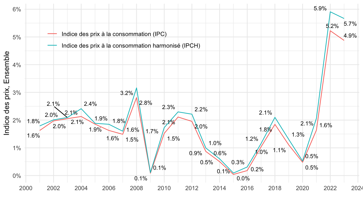
`IPCH-2015` |>
  bind_rows(`IPC-2015`) |>
  filter(COICOP2016 %in% c("00"),
         NATURE == "INDICE",
         REF_AREA == "FE",
         FREQ == "A",
         is.na(MENAGES_IPC) | MENAGES_IPC == "ENSEMBLE",
         is.na(PRIX_CONSO) | PRIX_CONSO == "SO") |>
  year_to_date() |>
  filter(date >= Sys.Date() - years(17)) |>

  group_by(INDICATEUR) |>
  arrange(date) |>
  mutate(OBS_VALUE = OBS_VALUE/lag(OBS_VALUE)-1) |>
  select(date, OBS_VALUE, INDICATEUR) |>
  na.omit() |>
  ggplot() + ylab("Indice des prix, Ensemble") + xlab("") + theme_minimal() +
  geom_line(aes(x = date, y = OBS_VALUE, color = INDICATEUR)) +
  #
  theme(legend.position = c(0.3, 0.8),
        legend.title = element_blank()) +
  scale_x_date(breaks = seq(1920, 2100, 1) |> paste0("-01-01") |> as.Date(),
               labels = date_format("%Y")) +
  scale_y_continuous(breaks = 0.01*seq(-10, 10, 1),
                     labels = percent_format()) +
  geom_text_repel(aes(x = date, y = OBS_VALUE, label = percent(OBS_VALUE, acc = 0.1), color = INDICATEUR),
                  fontface ="plain", size = 3)
`IPCH-2015` |>
  bind_rows(`IPC-2015`) |>
  filter(COICOP2016 %in% c("00"),
         NATURE == "INDICE",
         REF_AREA == "FE",
         FREQ == "A",
         is.na(MENAGES_IPC) | MENAGES_IPC == "ENSEMBLE",
         is.na(PRIX_CONSO) | PRIX_CONSO == "SO") |>
  year_to_date() |>

  group_by(INDICATEUR) |>
  arrange(date) |>
  mutate(OBS_VALUE = OBS_VALUE/lag(OBS_VALUE)-1) |>
  filter(date >= as.Date("2017-01-01")) |>
  select(date, OBS_VALUE, INDICATEUR) |>
  na.omit() |>
  ggplot() + ylab("Indice des prix, Ensemble") + xlab("") + theme_minimal() +
  geom_line(aes(x = date, y = OBS_VALUE, color = INDICATEUR)) +
  #
  theme(legend.position = c(0.3, 0.8),
        legend.title = element_blank()) +
  scale_x_date(breaks = seq(1920, 2100, 1) |> paste0("-01-01") |> as.Date(),
               labels = date_format("%Y")) +
  scale_y_continuous(breaks = 0.01*seq(-10, 10, 1),
                     labels = percent_format()) +
  geom_text_repel(aes(x = date, y = OBS_VALUE, label = percent(OBS_VALUE, acc = 0.1), color = INDICATEUR),
                  fontface ="plain", size = 3, show.legend = F)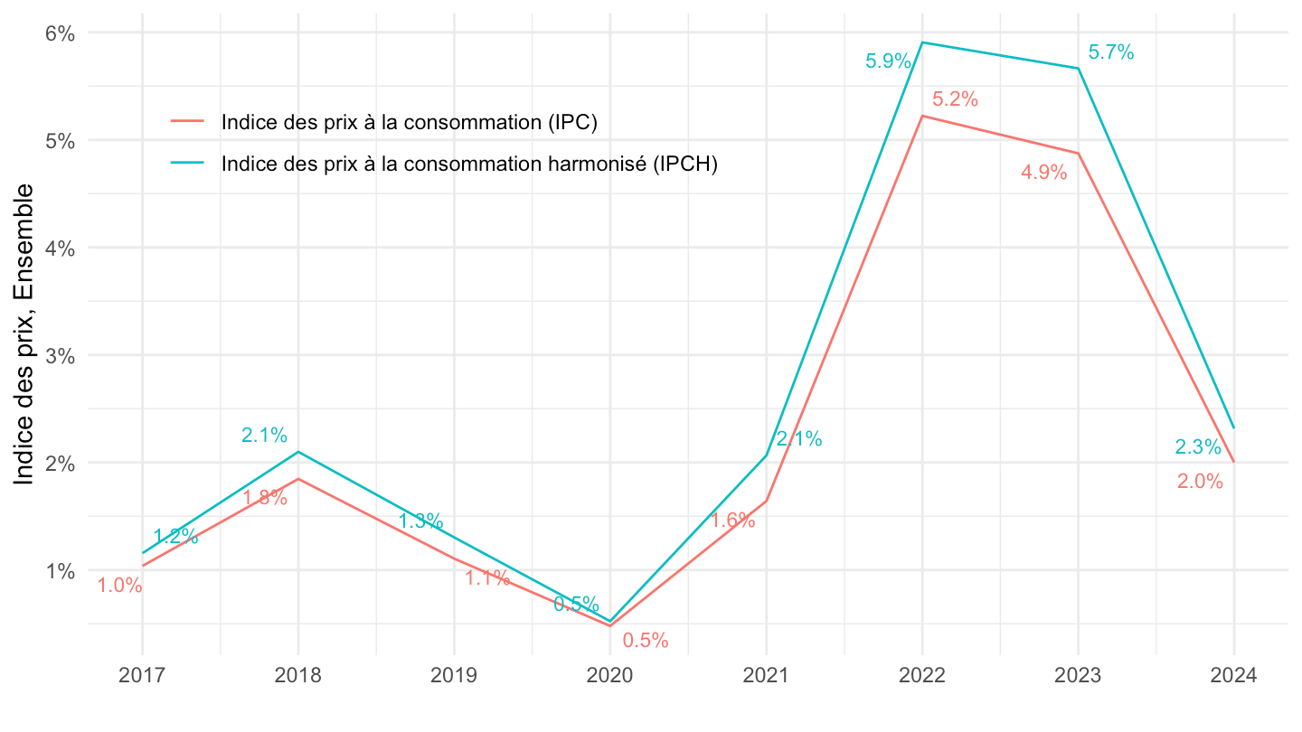
`IPCH-IPC-2015-ensemble` |>
  filter(date >= as.Date("2017-01-01")) |>
  group_by(Indicateur) |>
  arrange(date) |>
  mutate(OBS_VALUE = 100*OBS_VALUE/OBS_VALUE[1]) |>
  ggplot() + ylab("Indice des prix, Ensemble") + xlab("") + theme_minimal() +
  geom_line(aes(x = date, y = OBS_VALUE, color = Indicateur)) +

  scale_x_date(breaks = seq(1920, 2100, 1) |> paste0("-01-01") |> as.Date(),
               labels = date_format("%Y")) +
  theme(legend.position = c(0.7, 0.2),
        legend.title = element_blank()) +
  scale_y_log10(breaks = seq(10, 300, 5),
                     labels = dollar_format(accuracy = 1, prefix = "")) +
  geom_label(data = . %>% tail(1), aes(x = date, y = OBS_VALUE, label = round(OBS_VALUE, 1)))
`IPCH-IPC-2015-ensemble` |>
  filter(date >= as.Date("2019-05-01")) |>
  group_by(Indicateur) |>
  arrange(date) |>
  mutate(OBS_VALUE = 100*OBS_VALUE/OBS_VALUE[1]) |>
  ggplot() + ylab("Indice des prix, Ensemble") + xlab("") + theme_minimal() +
  geom_line(aes(x = date, y = OBS_VALUE, color = Indicateur)) +

  scale_x_date(breaks = seq(1920, 2100, 1) |> paste0("-01-01") |> as.Date(),
               labels = date_format("%Y")) +
  theme(legend.position = c(0.3, 0.8),
        legend.title = element_blank()) +
  scale_y_log10(breaks = seq(10, 300, 1),
                     labels = dollar_format(accuracy = 1, prefix = "")) +
  geom_label(data = . %>%
               filter(date == max(date)), aes(date, y = OBS_VALUE, label = round(OBS_VALUE, 1)))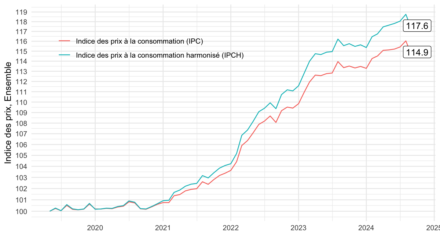
`IPCH-IPC-2015-ensemble` |>
  filter(date >= as.Date("2021-01-01")) |>
  group_by(Indicateur) |>
  arrange(date) |>
  mutate(OBS_VALUE = 100*OBS_VALUE/OBS_VALUE[1]) |>
  ggplot() + ylab("Indice des prix, Ensemble") + xlab("") + theme_minimal() +
  geom_line(aes(x = date, y = OBS_VALUE, color = Indicateur)) +

  scale_x_date(breaks = seq(1920, 2100, 1) |> paste0("-01-01") |> as.Date(),
               labels = date_format("%Y")) +
  theme(legend.position = c(0.3, 0.8),
        legend.title = element_blank()) +
  scale_y_log10(breaks = seq(10, 300, 1),
                     labels = dollar_format(accuracy = 1, prefix = "")) +
  geom_label(data = . %>%
               filter(date == max(date)), aes(date, y = OBS_VALUE, label = round(OBS_VALUE, 1)))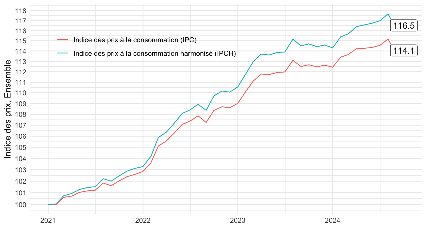
`IPCH-IPC-2015-ensemble` |>
  filter(date >= as.Date("2018-11-01")) |>
  group_by(Indicateur) |>
  arrange(date) |>
  mutate(OBS_VALUE = 100*OBS_VALUE/OBS_VALUE[1]) |>
  ggplot() + ylab("Indice des prix, Ensemble") + xlab("") + theme_minimal() +
  geom_line(aes(x = date, y = OBS_VALUE, color = Indicateur)) +

  scale_x_date(breaks = seq(1920, 2100, 1) |> paste0("-01-01") |> as.Date(),
               labels = date_format("%Y")) +
  theme(legend.position = c(0.3, 0.8),
        legend.title = element_blank()) +
  scale_y_log10(breaks = seq(10, 300, 1),
                     labels = dollar_format(accuracy = 1, prefix = "")) +
  geom_label(data = . %>%
               filter(date == max(date)), aes(date, y = OBS_VALUE, label = round(OBS_VALUE, 1), color = Indicateur))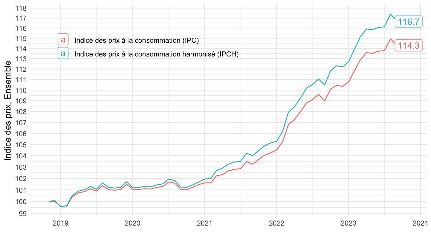
`IPCH-IPC-2015-ensemble` |>
  filter(date >= as.Date("2021-06-01")) |>
  group_by(Indicateur) |>
  arrange(date) |>
  mutate(OBS_VALUE = 100*OBS_VALUE/OBS_VALUE[1]) |>
  ggplot() + ylab("Indice des prix, Ensemble") + xlab("") + theme_minimal() +
  geom_line(aes(x = date, y = OBS_VALUE, color = Indicateur)) +

  scale_x_date(breaks = seq(1920, 2100, 1) |> paste0("-01-01") |> as.Date(),
               labels = date_format("%Y")) +
  theme(legend.position = c(0.3, 0.8),
        legend.title = element_blank()) +
  scale_y_log10(breaks = seq(10, 300, 1),
                     labels = dollar_format(accuracy = 1, prefix = "")) +
  geom_label(data = . %>%
               filter(date == max(date)), aes(date, y = OBS_VALUE, label = round(OBS_VALUE, 1)))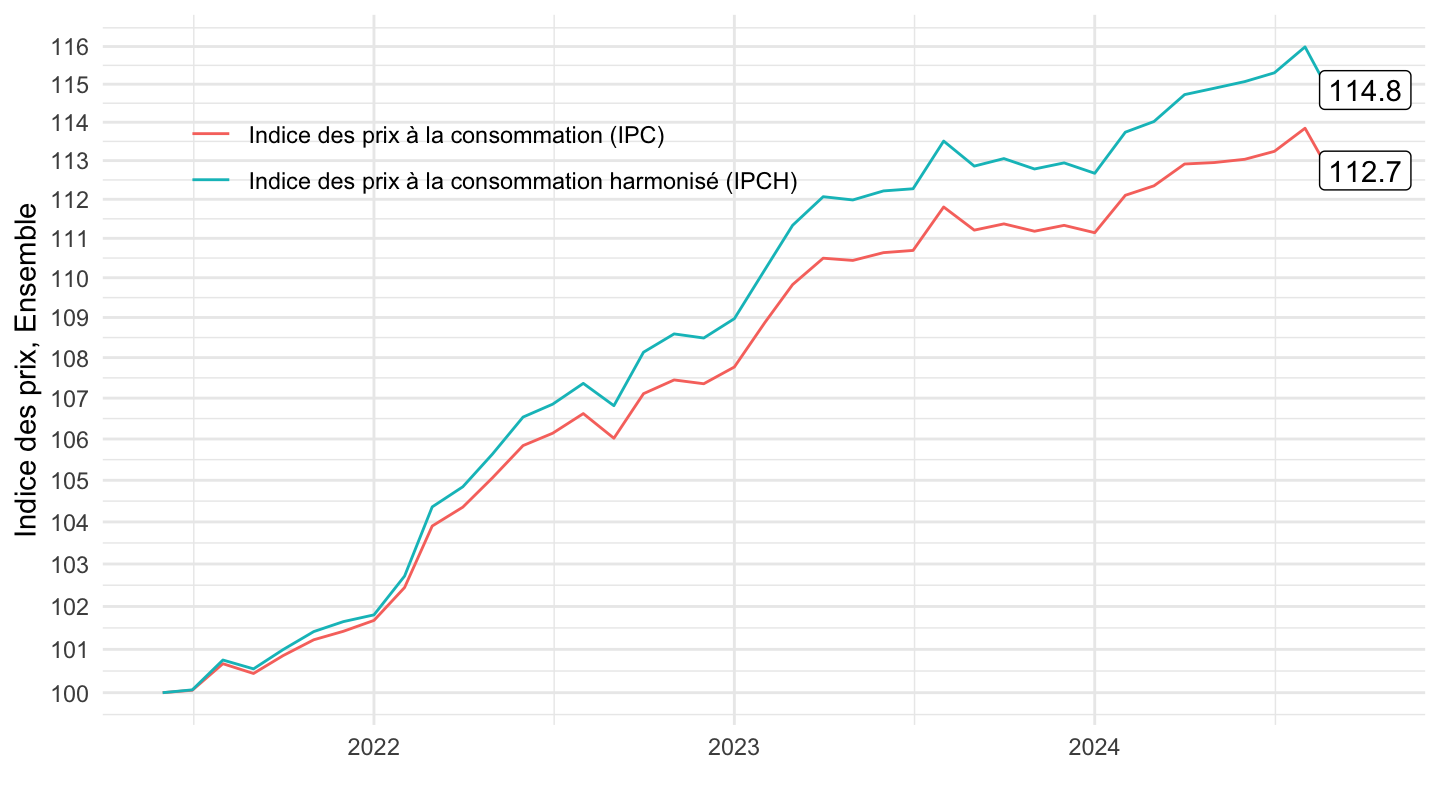
`IPCH-IPC-2015-ensemble` |>
  filter(date >= as.Date("2014-12-01"),
         year(date) <= 2024) |>
  group_by(Indicateur) |>
  mutate(OBS_VALUE = 100*OBS_VALUE/OBS_VALUE[1]) |>
  ggplot() + ylab("Indice des prix, Ensemble") + xlab("") + theme_minimal() +
  geom_line(aes(x = date, y = OBS_VALUE, color = Indicateur)) +

  scale_x_date(breaks = seq(2000, 2100, 2) |> paste0("-01-01") |> as.Date(),
               labels = date_format("%Y")) +
  theme(legend.position = c(0.7, 0.2),
        legend.title = element_blank()) +
  scale_y_log10(breaks = seq(10, 300, 5),
                     labels = dollar_format(accuracy = 1, prefix = "")) +
  geom_label(data = . %>%
               filter(date == max(date)), aes(date, y = OBS_VALUE, label = round(OBS_VALUE, 1), color = Indicateur))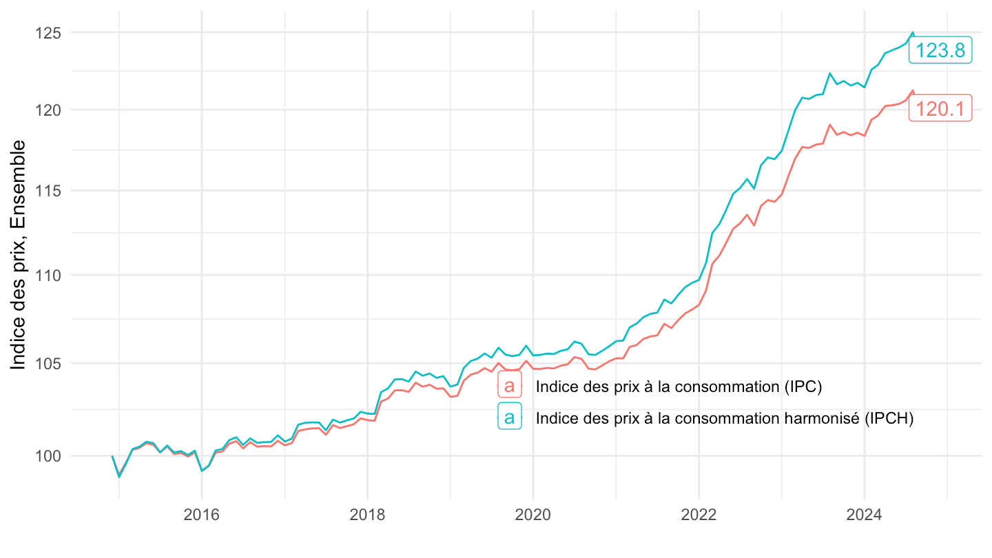
`IPCH-2015` |>
  bind_rows(`IPC-2015`) |>
  filter(COICOP2016 %in% c("00"),
         NATURE == "INDICE",
         REF_AREA == "FE",
         FREQ == "A",
         is.na(MENAGES_IPC) | MENAGES_IPC == "ENSEMBLE",
         is.na(PRIX_CONSO) | PRIX_CONSO == "SO") |>
  year_to_date() |>
  filter(date >= as.Date("2000-01-01"),
         date <= as.Date("2024-12-01")) |>

  group_by(INDICATEUR) |>
  arrange(date) |>
  mutate(OBS_VALUE = 100*OBS_VALUE/OBS_VALUE[date == as.Date("2000-01-01")]) |>
  ggplot() + ylab("Indice des prix, Ensemble") + xlab("") + theme_minimal() +
  geom_line(aes(x = date, y = OBS_VALUE, color = INDICATEUR)) +

  theme(legend.position = c(0.7, 0.2),
        legend.title = element_blank()) +
  scale_x_date(breaks = seq(1920, 2100, 2) |> paste0("-01-01") |> as.Date(),
               labels = date_format("%Y")) +
  scale_y_log10(breaks = seq(10, 300, 2),
                     labels = dollar_format(accuracy = 1, prefix = "")) +
  geom_label(data = . %>% filter(date == max(date)), aes(x = date, y = OBS_VALUE, label = round(OBS_VALUE, 1), color = INDICATEUR))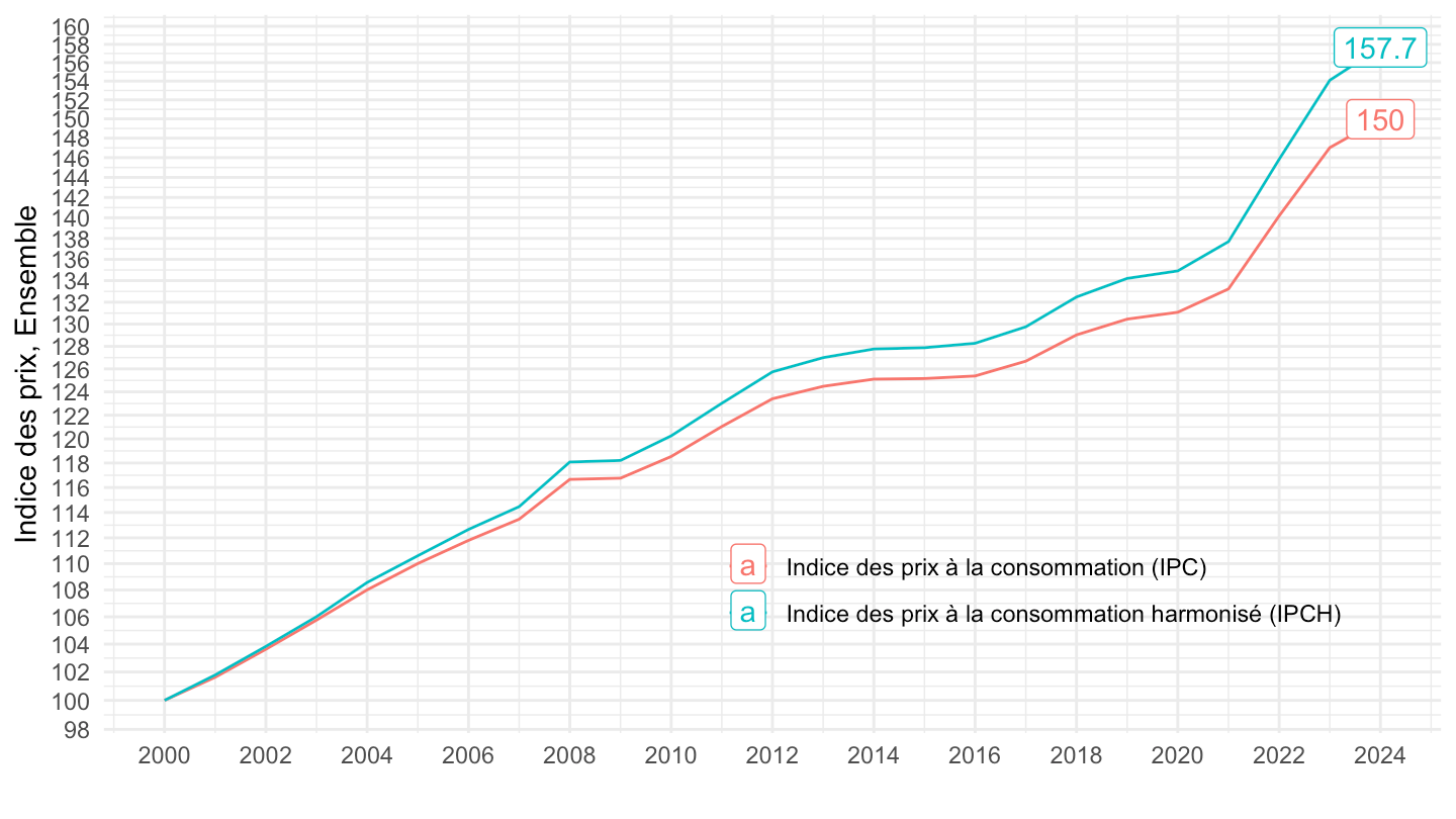
`IPCH-IPC-2015-ensemble` |>
  filter(year(date) >= 2000,
         year(date) <= 2024) |>
  group_by(Indicateur) |>
  mutate(OBS_VALUE = 100*OBS_VALUE/OBS_VALUE[1]) |>
  ggplot() + ylab("Indice des prix, Ensemble") + xlab("") + theme_minimal() +
  geom_line(aes(x = date, y = OBS_VALUE, color = Indicateur)) +

  scale_x_date(breaks = seq(2000, 2100, 2) |> paste0("-01-01") |> as.Date(),
               labels = date_format("%Y")) +
  theme(legend.position = c(0.7, 0.2),
        legend.title = element_blank()) +
  scale_y_log10(breaks = seq(10, 300, 5),
                     labels = dollar_format(accuracy = 1, prefix = "")) +
  geom_label(data = . %>%
               filter(date == max(date)), aes(date, y = OBS_VALUE, label = round(OBS_VALUE, 1), color = Indicateur))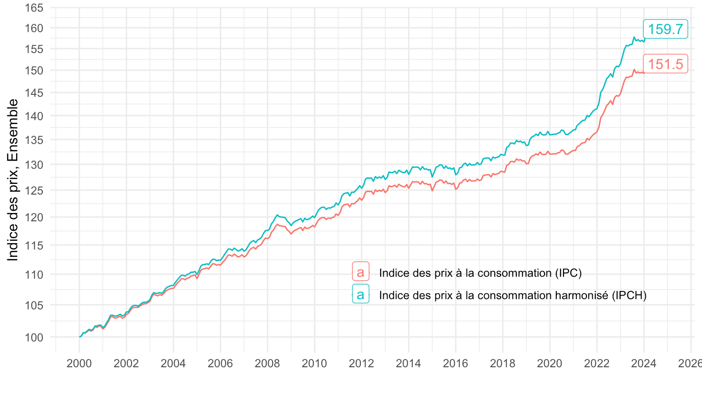
`IPCH-2015` |>
  bind_rows(`IPC-2015`) |>
  filter(COICOP2016 %in% c("00"),
         NATURE == "INDICE",
         REF_AREA == "FE",
         FREQ == "A",
         is.na(MENAGES_IPC) | MENAGES_IPC == "ENSEMBLE",
         is.na(PRIX_CONSO) | PRIX_CONSO == "SO") |>
  year_to_date() |>
  filter(date >= as.Date("2000-01-01"),
         date <= as.Date("2024-12-01")) |>

  group_by(INDICATEUR) |>
  arrange(date) |>
  mutate(OBS_VALUE = 100*OBS_VALUE/OBS_VALUE[date == as.Date("2000-01-01")]) |>
  ggplot() + ylab("Indice des prix, Ensemble") + xlab("") + theme_minimal() +
  geom_line(aes(x = date, y = OBS_VALUE, color = INDICATEUR)) +

  theme(legend.position = c(0.7, 0.2),
        legend.title = element_blank()) +
  scale_x_date(breaks = seq(1920, 2100, 2) |> paste0("-01-01") |> as.Date(),
               labels = date_format("%Y")) +
  scale_y_log10(breaks = seq(10, 300, 2),
                     labels = dollar_format(accuracy = 1, prefix = "")) +
  geom_label(data = . %>% filter(date == max(date)), aes(x = date, y = OBS_VALUE, label = round(OBS_VALUE, 1), color = INDICATEUR))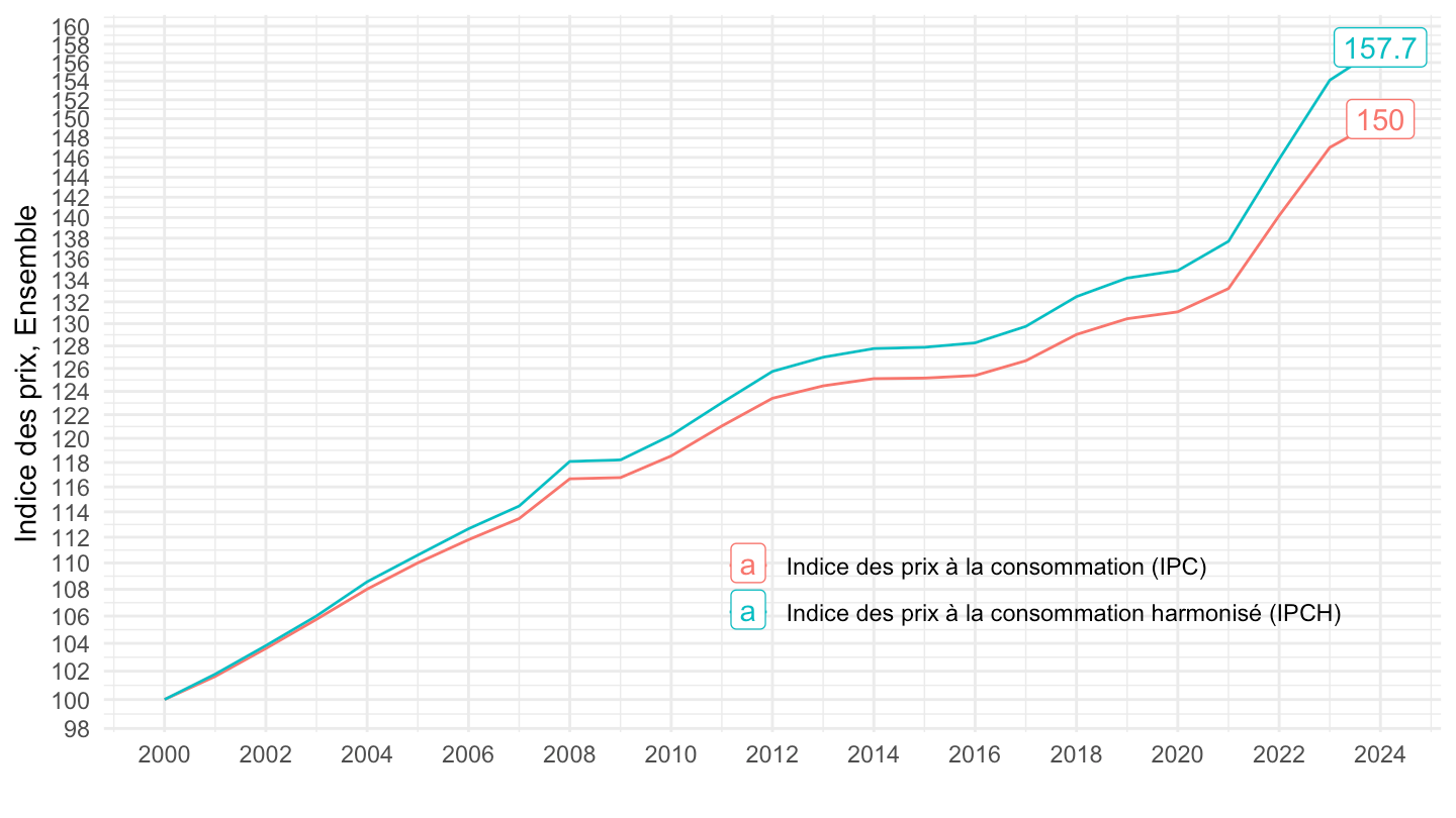
`IPCH-IPC-2015-ensemble` |>
  filter(year(date) >= 1999) |>
  group_by(Indicateur) |>
  mutate(OBS_VALUE = 100*OBS_VALUE/OBS_VALUE[1]) |>
  ggplot() + ylab("Indice des prix, Ensemble") + xlab("") + theme_minimal() +
  geom_line(aes(x = date, y = OBS_VALUE, color = Indicateur)) +

  scale_x_date(breaks = seq(1999, 2100, 5) |> paste0("-01-01") |> as.Date(),
               labels = date_format("%Y")) +
  theme(legend.position = c(0.7, 0.2),
        legend.title = element_blank()) +
  scale_y_log10(breaks = seq(10, 300, 5),
                     labels = dollar_format(accuracy = 1, prefix = "")) +
  geom_label(data = . %>%
               filter(date == max(date)), aes(date, y = OBS_VALUE, label = round(OBS_VALUE, 1), color = Indicateur))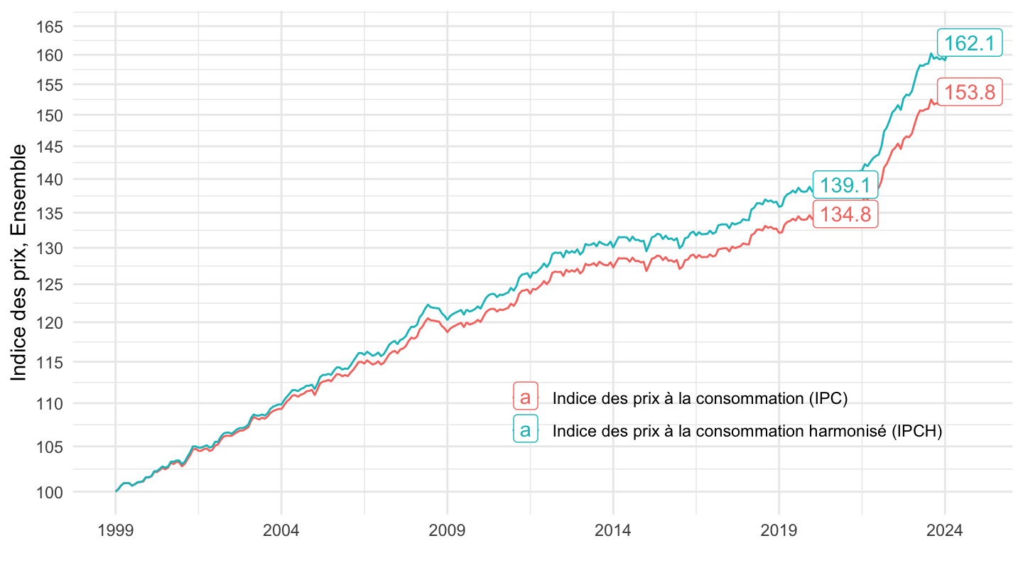
`IPCH-IPC-2015-ensemble` |>
  filter(date >= as.Date("2016-01-01")) |>
  group_by(Indicateur) |>
  arrange(date) |>
  mutate(OBS_VALUE = 100*OBS_VALUE/OBS_VALUE[1]) |>
  ggplot() + ylab("Indice des prix, Ensemble") + xlab("") + theme_minimal() +
  geom_line(aes(x = date, y = OBS_VALUE, color = Indicateur)) +

  scale_x_date(breaks = seq(1920, 2100, 1) |> paste0("-01-01") |> as.Date(),
               labels = date_format("%Y")) +
  theme(legend.position = c(0.3, 0.8),
        legend.title = element_blank()) +
  scale_y_log10(breaks = seq(10, 300, 2),
                     labels = dollar_format(accuracy = 1, prefix = "")) +
  geom_label(data = . %>%
               filter(date == max(date)), aes(date, y = OBS_VALUE, label = round(OBS_VALUE, 1), color = Indicateur))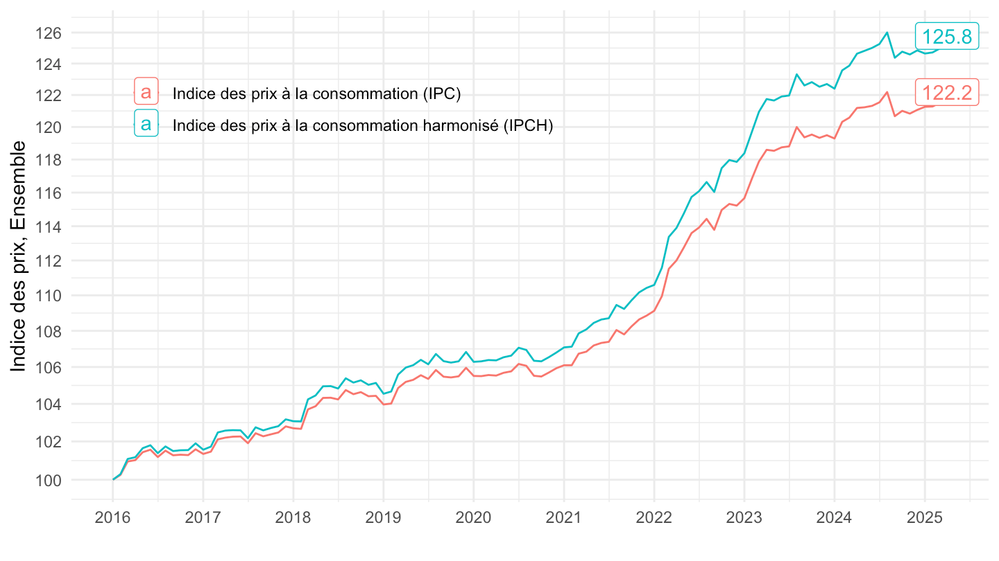
`IPCH-IPC-2015-ensemble` |>
  filter(date >+ as.Date("2008-01-01")) |>
  group_by(Indicateur) |>
  arrange(date) |>
  mutate(OBS_VALUE = 100*OBS_VALUE/OBS_VALUE[1]) |>
  ggplot() + ylab("Indice des prix, Ensemble") + xlab("") + theme_minimal() +
  geom_line(aes(x = date, y = OBS_VALUE, color = Indicateur)) +

  scale_x_date(breaks = seq(1920, 2100, 2) |> paste0("-01-01") |> as.Date(),
               labels = date_format("%Y")) +
  theme(legend.position = c(0.7, 0.2),
        legend.title = element_blank()) +
  scale_y_log10(breaks = seq(10, 300, 5),
                     labels = dollar_format(accuracy = 1, prefix = "")) +
  geom_label(data = . %>%
               filter(date == max(date)), aes(date, y = OBS_VALUE, label = round(OBS_VALUE, 1)))
`IPCH-IPC-2015-ensemble` |>
  ggplot() + ylab("Indice des prix, Ensemble") + xlab("") + theme_minimal() +
  geom_line(aes(x = date, y = OBS_VALUE, color = Indicateur)) +

  scale_x_date(breaks = seq(1920, 2100, 2) |> paste0("-01-01") |> as.Date(),
               labels = date_format("%Y")) +
  theme(legend.position = c(0.7, 0.2),
        legend.title = element_blank()) +
  scale_y_log10(breaks = seq(10, 300, 5),
                     labels = dollar_format(accuracy = 1, prefix = "")) +
  geom_label(data = . %>%
               filter(date == max(date)), aes(date, y = OBS_VALUE, label = round(OBS_VALUE, 1), color = Indicateur))
`IPCH-IPC-2015-ensemble` |>
  ggplot() + ylab("Indice des prix, Ensemble") + xlab("") + theme_minimal() +
  geom_line(aes(x = date, y = OBS_VALUE, color = Indicateur)) +

  scale_x_date(breaks = seq(1920, 2100, 2) |> paste0("-01-01") |> as.Date(),
               labels = date_format("%Y")) +
  theme(legend.position = c(0.7, 0.2),
        legend.title = element_blank()) +
  scale_y_log10(breaks = seq(10, 300, 5),
                     labels = dollar_format(accuracy = 1, prefix = "")) +
  geom_text_repel(data = . %>% filter(month(date) == 12),
                  aes(x = date, y = OBS_VALUE, label = round(OBS_VALUE, 1)),
                  fontface ="plain", color = "black", size = 3)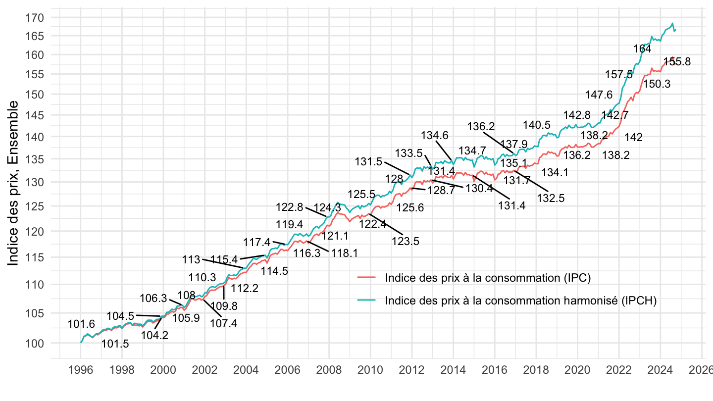
`IPCH-IPC-2015-ensemble` |>
  select(date, INDICATEUR, OBS_VALUE) |>
  spread(INDICATEUR, OBS_VALUE) |>
  mutate(OBS_VALUE = 100*IPCH/IPC) |>
  filter(date >= as.Date("1999-01-01")) |>
  mutate(OBS_VALUE = 100*OBS_VALUE/OBS_VALUE[1]) |>
  ggplot() + ylab("Ratio IPCH/IPC") + xlab("") + theme_minimal() +
  geom_line(aes(x = date, y = OBS_VALUE)) +
  scale_x_date(breaks = seq(1920, 2100, 2) |> paste0("-01-01") |> as.Date(),
               labels = date_format("%Y")) +
  theme(legend.position = c(0.7, 0.2),
        legend.title = element_blank()) +
  scale_y_log10(breaks = seq(10, 300, 1),
                     labels = dollar_format(accuracy = 1, prefix = ""))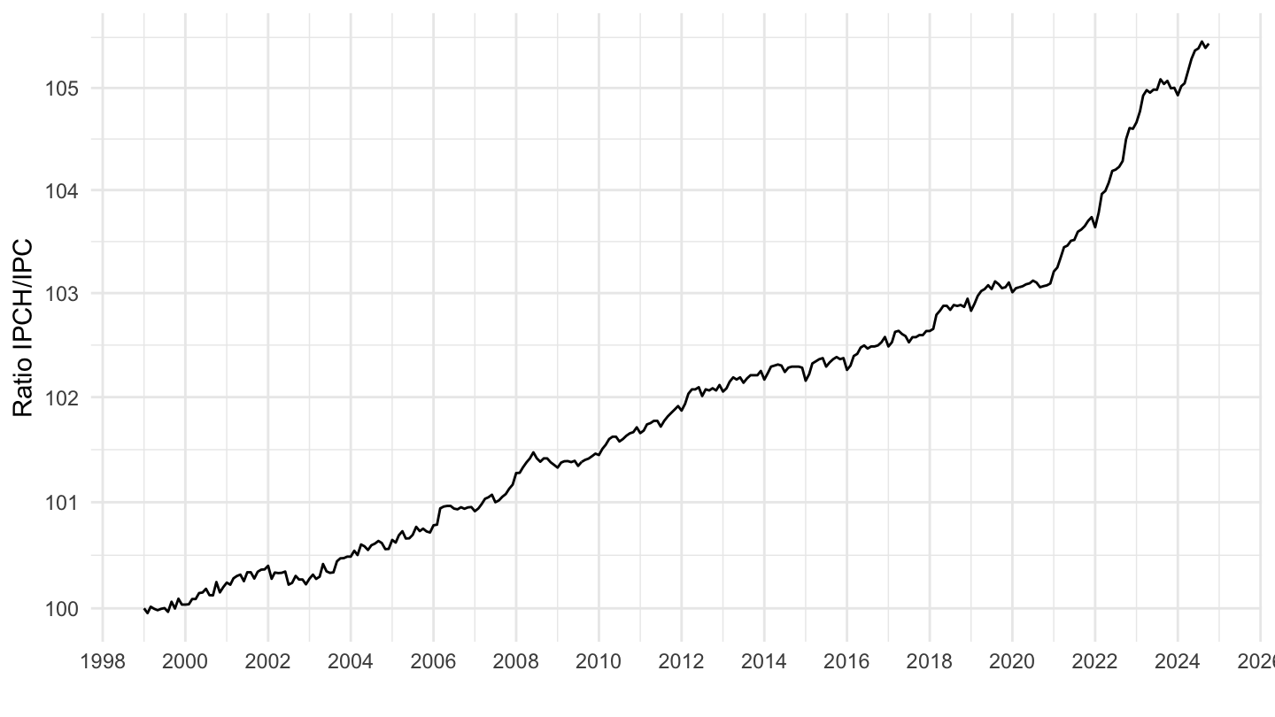
`IPCH-IPC-2015-ensemble` |>
  select(date, INDICATEUR, OBS_VALUE) |>
  spread(INDICATEUR, OBS_VALUE) |>
  mutate(OBS_VALUE = 100*IPCH/IPC) |>
  ggplot() + ylab("Ratio IPCH/IPC") + xlab("") + theme_minimal() +
  geom_line(aes(x = date, y = OBS_VALUE)) +
  scale_x_date(breaks = seq(1920, 2100, 2) |> paste0("-01-01") |> as.Date(),
               labels = date_format("%Y")) +
  theme(legend.position = c(0.7, 0.2),
        legend.title = element_blank()) +
  scale_y_log10(breaks = seq(10, 300, 1),
                     labels = dollar_format(accuracy = 1, prefix = ""))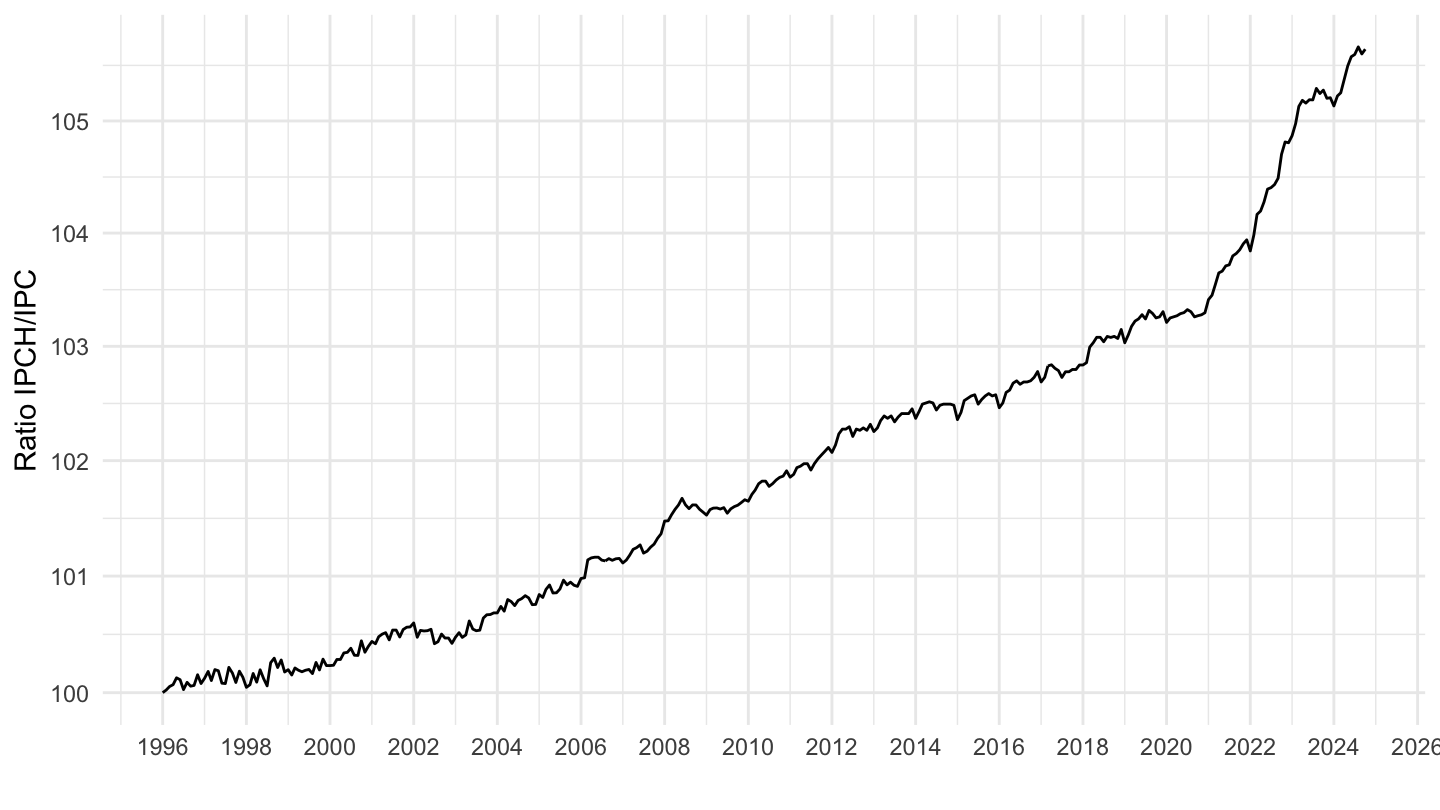
`IPCH-IPC-2015-ensemble` |>
  select(date, INDICATEUR, OBS_VALUE) |>
  spread(INDICATEUR, OBS_VALUE) |>
  mutate(OBS_VALUE = 100*IPC/IPCH) |>
  ggplot() + ylab("Ratio IPC/IPCH") + xlab("") + theme_minimal() +
  geom_line(aes(x = date, y = OBS_VALUE)) +
  scale_x_date(breaks = seq(1920, 2100, 2) |> paste0("-01-01") |> as.Date(),
               labels = date_format("%Y")) +
  theme(legend.position = c(0.7, 0.2),
        legend.title = element_blank()) +
  scale_y_log10(breaks = seq(10, 300, 1),
                     labels = dollar_format(accuracy = 1, prefix = ""))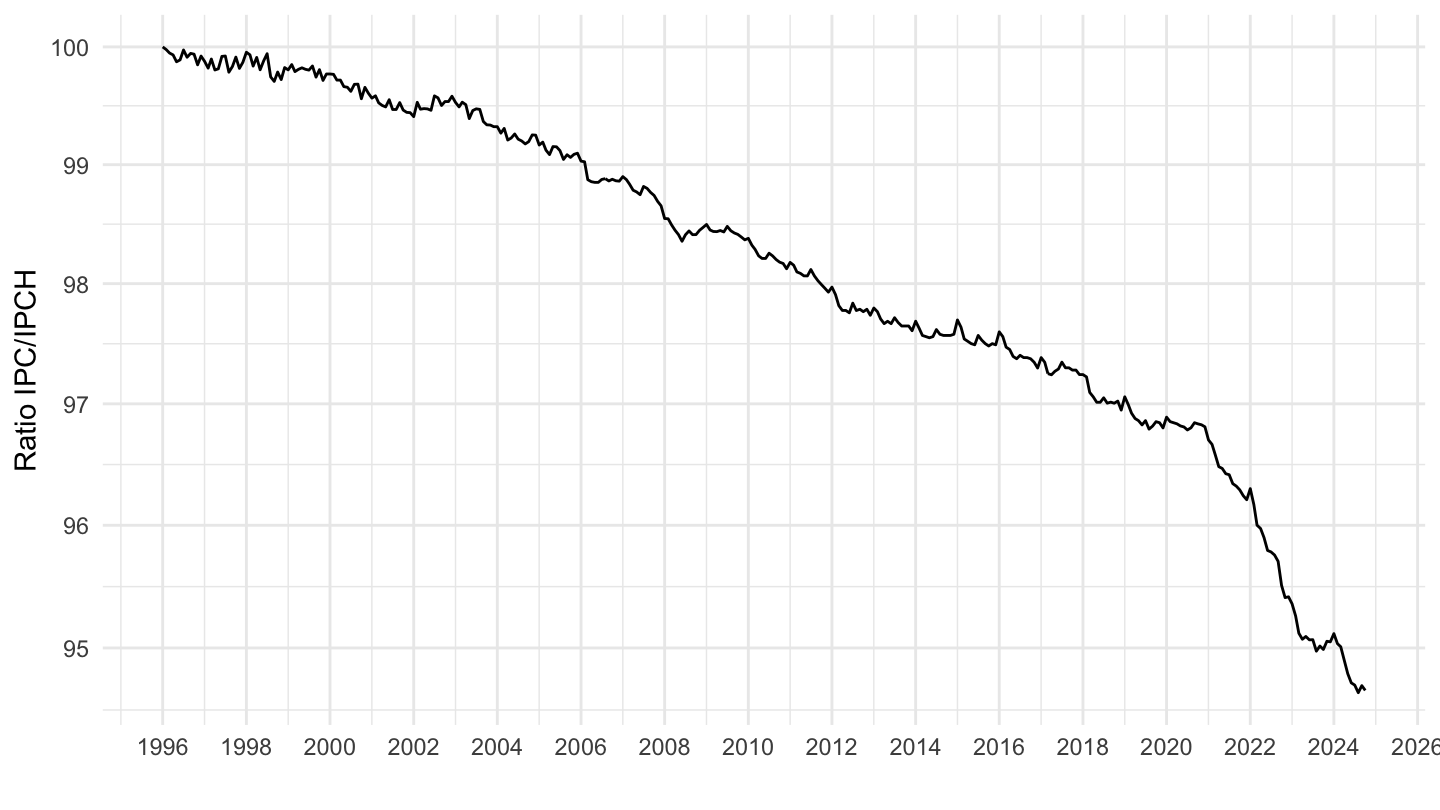
`IPCH-IPC-2015-ensemble` |>
  select(date, INDICATEUR, OBS_VALUE) |>
  spread(INDICATEUR, OBS_VALUE) |>
  mutate(OBS_VALUE = 100*IPC/IPCH) |>
  filter(date >= as.Date("1999-01-01")) |>
  mutate(OBS_VALUE = 100*OBS_VALUE/OBS_VALUE[1]) |>
  ggplot() + ylab("Ratio IPC/IPCH") + xlab("") + theme_minimal() +
  geom_line(aes(x = date, y = OBS_VALUE)) +
  scale_x_date(breaks = seq(1920, 2100, 2) |> paste0("-01-01") |> as.Date(),
               labels = date_format("%Y")) +
  theme(legend.position = c(0.7, 0.2),
        legend.title = element_blank()) +
  scale_y_log10(breaks = seq(10, 300, 1),
                     labels = dollar_format(accuracy = 1, prefix = ""))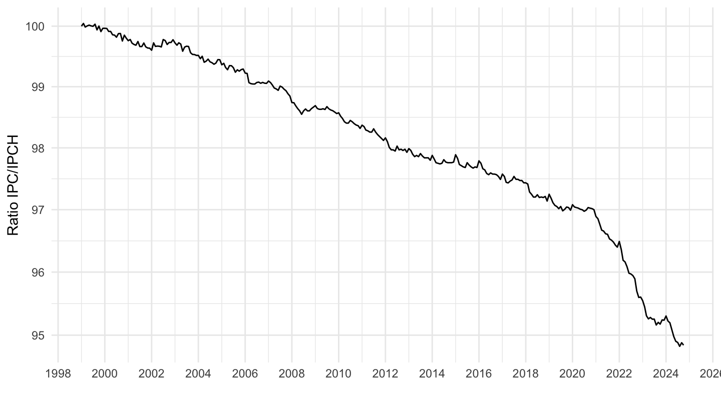
`IPCH-2015` |>
  bind_rows(`IPC-2015`) |>
  filter(COICOP2016 %in% c("00"),
         NATURE == "INDICE",
         REF_AREA == "FE",
         FREQ == "A",
         is.na(MENAGES_IPC) | MENAGES_IPC == "ENSEMBLE",
         is.na(PRIX_CONSO) | PRIX_CONSO == "SO") |>
  year_to_date() |>
  filter(date >= as.Date("1996-01-01")) |>

  group_by(INDICATEUR) |>
  arrange(date) |>
  mutate(OBS_VALUE = 100*OBS_VALUE/OBS_VALUE[date == as.Date("1996-01-01")]) |>
  ggplot() + ylab("Indice des prix, Ensemble") + xlab("") + theme_minimal() +
  geom_line(aes(x = date, y = OBS_VALUE, color = INDICATEUR)) +

  theme(legend.position = c(0.7, 0.2),
        legend.title = element_blank()) +
  scale_x_date(breaks = seq(1920, 2100, 2) |> paste0("-01-01") |> as.Date(),
               labels = date_format("%Y")) +
  scale_y_log10(breaks = seq(10, 300, 5),
                     labels = dollar_format(accuracy = 1, prefix = "")) +
  geom_label(data = . %>% filter(date == max(date)), aes(x = date, y = OBS_VALUE, label = round(OBS_VALUE, 1), color = INDICATEUR))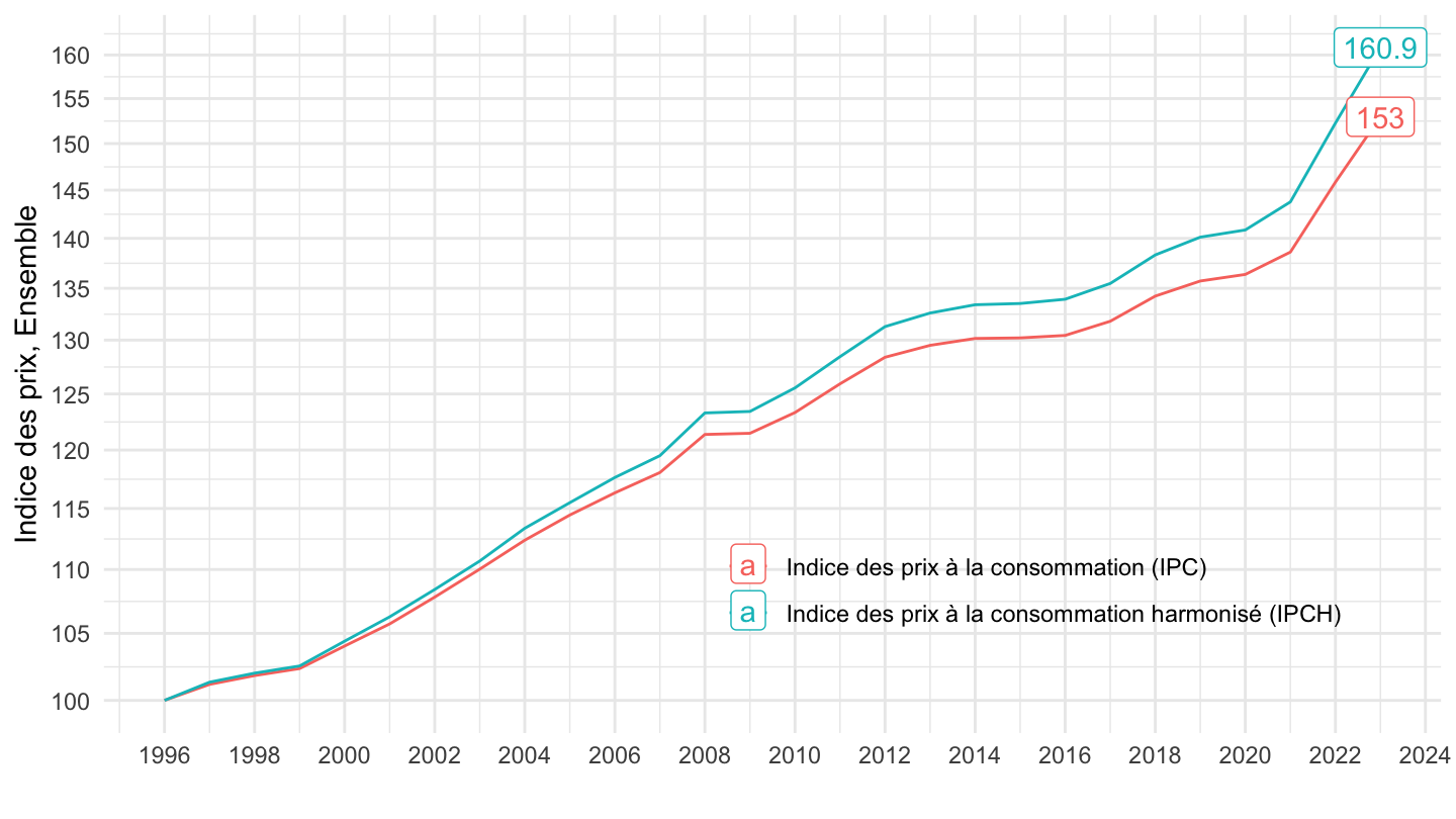
`IPCH-2015` |>
  bind_rows(`IPC-2015`) |>
  filter(COICOP2016 %in% c("00"),
         NATURE == "INDICE",
         REF_AREA == "FE",
         FREQ == "A",
         is.na(MENAGES_IPC) | MENAGES_IPC == "ENSEMBLE",
         is.na(PRIX_CONSO) | PRIX_CONSO == "SO") |>
  year_to_date() |>
  filter(date >= as.Date("2008-01-01"),
         date <= as.Date("2022-01-01")) |>

  group_by(INDICATEUR) |>
  arrange(date) |>
  mutate(OBS_VALUE = 100*OBS_VALUE/OBS_VALUE[date == as.Date("2008-01-01")]) |>
  ggplot() + ylab("Indice des prix, Ensemble") + xlab("") + theme_minimal() +
  geom_line(aes(x = date, y = OBS_VALUE, color = INDICATEUR)) +

  theme(legend.position = c(0.7, 0.2),
        legend.title = element_blank()) +
  scale_x_date(breaks = seq(1920, 2100, 2) |> paste0("-01-01") |> as.Date(),
               labels = date_format("%Y")) +
  scale_y_log10(breaks = seq(10, 300, 5),
                     labels = dollar_format(accuracy = 1, prefix = "")) +
  geom_label(data = . %>% filter(date == max(date)), aes(x = date, y = OBS_VALUE, label = round(OBS_VALUE, 1), color = INDICATEUR))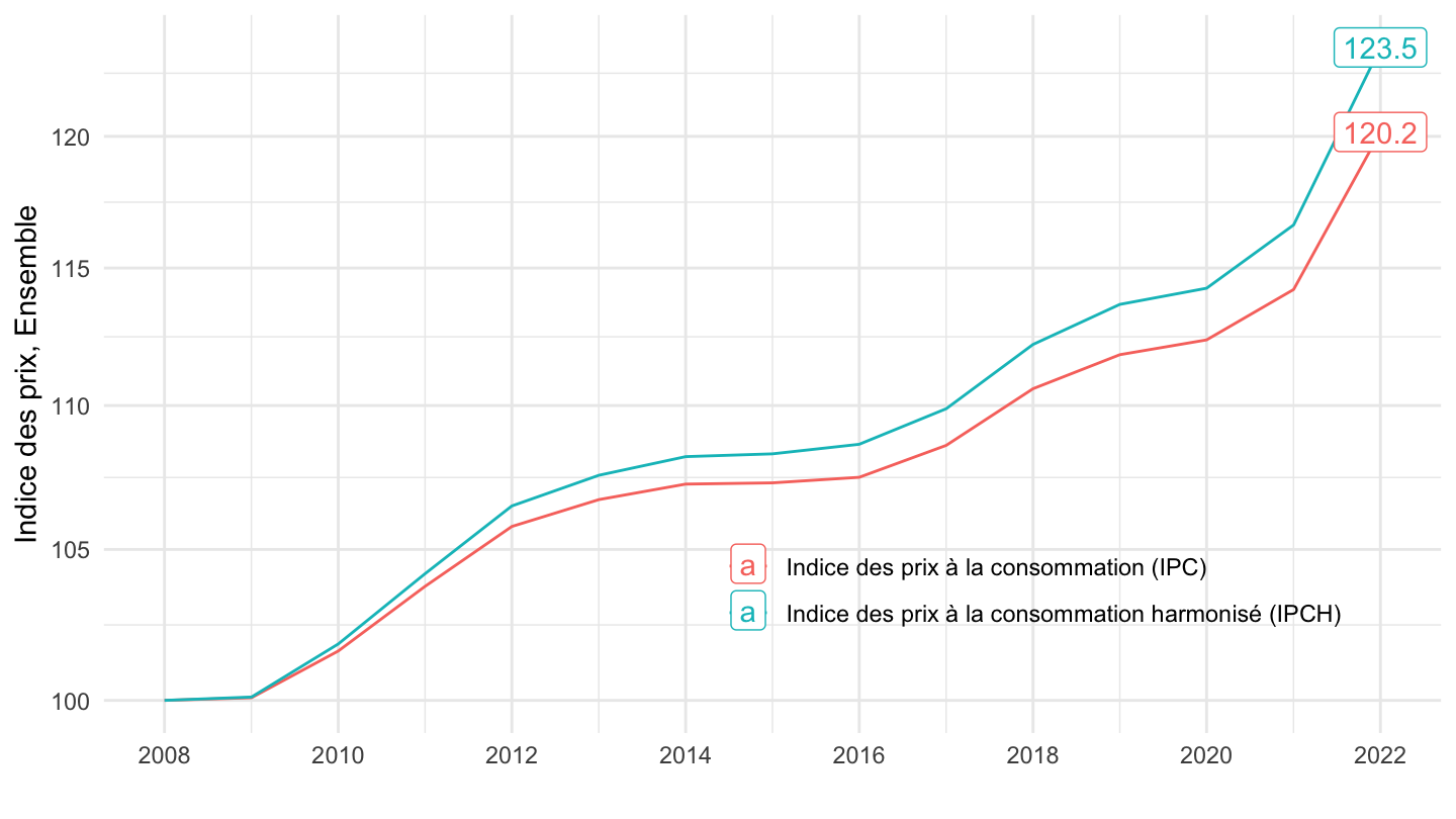
`IPCH-2015` |>
  bind_rows(`IPC-2015`) |>
  filter(COICOP2016 %in% c("00"),
         NATURE == "INDICE",
         REF_AREA == "FE",
         FREQ == "A",
         is.na(MENAGES_IPC) | MENAGES_IPC == "ENSEMBLE",
         is.na(PRIX_CONSO) | PRIX_CONSO == "SO") |>
  year_to_date() |>
  filter(date >= as.Date("2008-01-01"),
         date <= as.Date("2021-01-01")) |>

  group_by(INDICATEUR) |>
  arrange(date) |>
  mutate(OBS_VALUE = 100*OBS_VALUE/OBS_VALUE[date == as.Date("2008-01-01")]) |>
  ggplot() + ylab("Indice des prix, Ensemble") + xlab("") + theme_minimal() +
  geom_line(aes(x = date, y = OBS_VALUE, color = INDICATEUR)) +

  theme(legend.position = c(0.7, 0.2),
        legend.title = element_blank()) +
  scale_x_date(breaks = seq(1920, 2100, 1) |> paste0("-01-01") |> as.Date(),
               labels = date_format("%Y")) +
  scale_y_log10(breaks = seq(10, 300, 2),
                     labels = dollar_format(accuracy = 1, prefix = "")) +
  geom_label(data = . %>% filter(date == max(date)), aes(x = date, y = OBS_VALUE, label = round(OBS_VALUE, 1), color = INDICATEUR))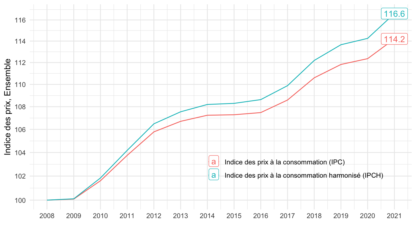
`IPCH-2015` |>
  bind_rows(`IPC-2015`) |>
  filter(COICOP2016 %in% c("00"),
         NATURE == "INDICE",
         REF_AREA == "FE",
         FREQ == "A",
         is.na(MENAGES_IPC) | MENAGES_IPC == "ENSEMBLE",
         is.na(PRIX_CONSO) | PRIX_CONSO == "SO") |>
  year_to_date() |>
  filter(date >= as.Date("2008-01-01"),
         date <= as.Date("2021-01-01")) |>

  group_by(INDICATEUR) |>
  arrange(date) |>
  mutate(OBS_VALUE = 100*OBS_VALUE/OBS_VALUE[date == as.Date("2008-01-01")]) |>
  ggplot() + ylab("Indice des prix, Ensemble") + xlab("") + theme_minimal() +
  geom_line(aes(x = date, y = OBS_VALUE, color = INDICATEUR)) +

  theme(legend.position = c(0.7, 0.2),
        legend.title = element_blank()) +
  scale_x_date(breaks = seq(1920, 2100, 1) |> paste0("-01-01") |> as.Date(),
               labels = date_format("%Y")) +
  scale_y_log10(breaks = seq(10, 300, 2),
                     labels = dollar_format(accuracy = 1, prefix = "")) +
  geom_label(data = . %>% filter(date == max(date)), aes(x = date, y = OBS_VALUE, label = round(OBS_VALUE, 2), color = INDICATEUR))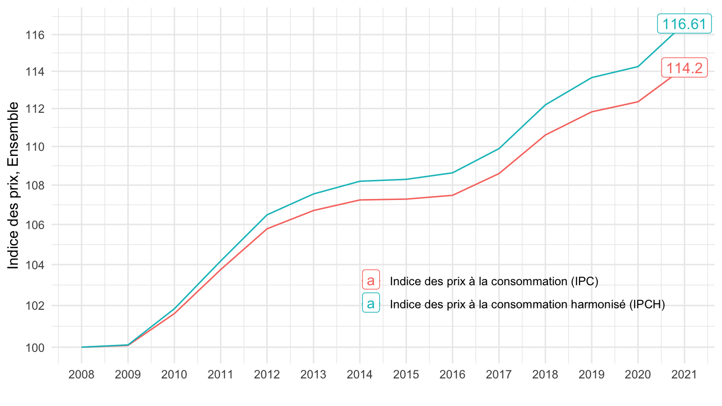
`IPCH-2015` |>
  bind_rows(`IPC-2015`) |>
  filter(COICOP2016 %in% c("00"),
         NATURE == "INDICE",
         REF_AREA == "FE",
         FREQ == "A",
         is.na(MENAGES_IPC) | MENAGES_IPC == "ENSEMBLE",
         is.na(PRIX_CONSO) | PRIX_CONSO == "SO") |>
  year_to_date() |>
  filter(date >= as.Date("1999-01-01")) |>

  group_by(INDICATEUR) |>
  arrange(date) |>
  mutate(OBS_VALUE = 100*OBS_VALUE/OBS_VALUE[date == as.Date("1999-01-01")]) |>
  ggplot() + ylab("Indice des prix, Ensemble") + xlab("") + theme_minimal() +
  geom_line(aes(x = date, y = OBS_VALUE, color = INDICATEUR)) +

  theme(legend.position = c(0.7, 0.2),
        legend.title = element_blank()) +
  scale_x_date(breaks = seq(1999, 2100, 5) |> paste0("-01-01") |> as.Date(),
               labels = date_format("%Y")) +
  scale_y_log10(breaks = seq(10, 300, 5),
                     labels = dollar_format(accuracy = 1, prefix = ""))
1996-
`IPCH-2015` |>
  bind_rows(`IPC-2015`) |>
  filter(COICOP2016 %in% c("00"),
         NATURE == "INDICE",
         REF_AREA == "FE",
         FREQ == "A",
         is.na(MENAGES_IPC) | MENAGES_IPC == "ENSEMBLE",
         is.na(PRIX_CONSO) | PRIX_CONSO == "SO") |>
  year_to_date() |>
  filter(date >= as.Date("1996-01-01")) |>

  group_by(INDICATEUR) |>
  arrange(date) |>
  mutate(OBS_VALUE = 100*OBS_VALUE/OBS_VALUE[date == as.Date("1996-01-01")]) |>
  ggplot() + ylab("Indice des prix, Ensemble") + xlab("") + theme_minimal() +
  geom_line(aes(x = date, y = OBS_VALUE, color = INDICATEUR)) +
  theme(legend.position = c(0.7, 0.2),
        legend.title = element_blank()) +
  scale_x_date(breaks = seq(1920, 2100, 2) |> paste0("-01-01") |> as.Date(),
               labels = date_format("%Y")) +
  scale_y_log10(breaks = seq(10, 300, 5),
                     labels = dollar_format(accuracy = 1, prefix = "")) +
  geom_text_repel(aes(x = date, y = OBS_VALUE, label = round(OBS_VALUE, 1)),
                  fontface ="plain", color = "black", size = 3)
2003-2022
`IPCH-2015` |>
  bind_rows(`IPC-2015`) |>
  filter(COICOP2016 %in% c("00"),
         NATURE == "INDICE",
         REF_AREA == "FE",
         FREQ == "A",
         is.na(MENAGES_IPC) | MENAGES_IPC == "ENSEMBLE",
         is.na(PRIX_CONSO) | PRIX_CONSO == "SO") |>
  year_to_date() |>
  filter(date >= as.Date("2003-01-01"),
         date <= as.Date("2022-01-01")) |>

  group_by(INDICATEUR) |>
  arrange(date) |>
  mutate(OBS_VALUE = 100*OBS_VALUE/OBS_VALUE[date == as.Date("2003-01-01")]) |>
  ggplot() + ylab("Indice des prix, Ensemble") + xlab("") + theme_minimal() +
  geom_line(aes(x = date, y = OBS_VALUE, color = INDICATEUR)) +
  theme(legend.position = c(0.7, 0.2),
        legend.title = element_blank()) +
  scale_x_date(breaks = seq(1920, 2100, 2) |> paste0("-01-01") |> as.Date(),
               labels = date_format("%Y")) +
  scale_y_log10(breaks = seq(10, 300, 5),
                     labels = dollar_format(accuracy = 1, prefix = "")) +
  geom_text_repel(aes(x = date, y = OBS_VALUE, label = round(OBS_VALUE, 1)),
                  fontface ="plain", color = "black", size = 3)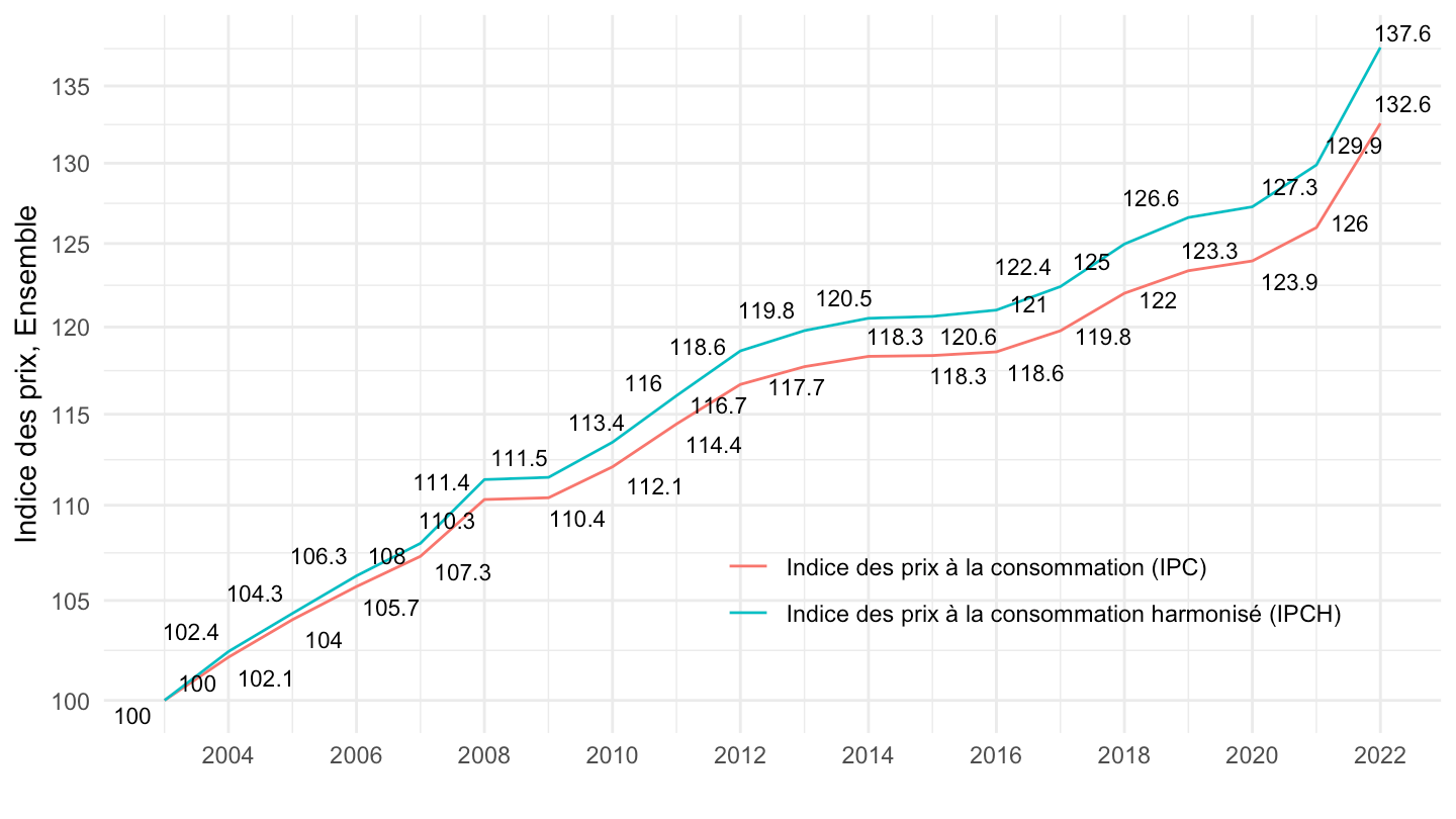
1999-
`IPCH-2015` |>
  bind_rows(`IPC-2015`) |>
  filter(COICOP2016 %in% c("00"),
         NATURE == "INDICE",
         REF_AREA == "FE",
         FREQ == "A",
         is.na(MENAGES_IPC) | MENAGES_IPC == "ENSEMBLE",
         is.na(PRIX_CONSO) | PRIX_CONSO == "SO") |>
  year_to_date() |>
  filter(date >= as.Date("1999-01-01")) |>

  group_by(INDICATEUR) |>
  arrange(date) |>
  mutate(OBS_VALUE = 100*OBS_VALUE/OBS_VALUE[date == as.Date("1999-01-01")]) |>
  ggplot() + ylab("Indice des prix, Ensemble") + xlab("") + theme_minimal() +
  geom_line(aes(x = date, y = OBS_VALUE, color = INDICATEUR)) +
  theme(legend.position = c(0.7, 0.2),
        legend.title = element_blank()) +
  scale_x_date(breaks = seq(1999, 2100, 5) |> paste0("-01-01") |> as.Date(),
               labels = date_format("%Y")) +
  scale_y_log10(breaks = seq(10, 300, 5),
                     labels = dollar_format(accuracy = 1, prefix = "")) +
  geom_text_repel(aes(x = date, y = OBS_VALUE, label = round(OBS_VALUE, 1)),
                  fontface ="plain", color = "black", size = 3)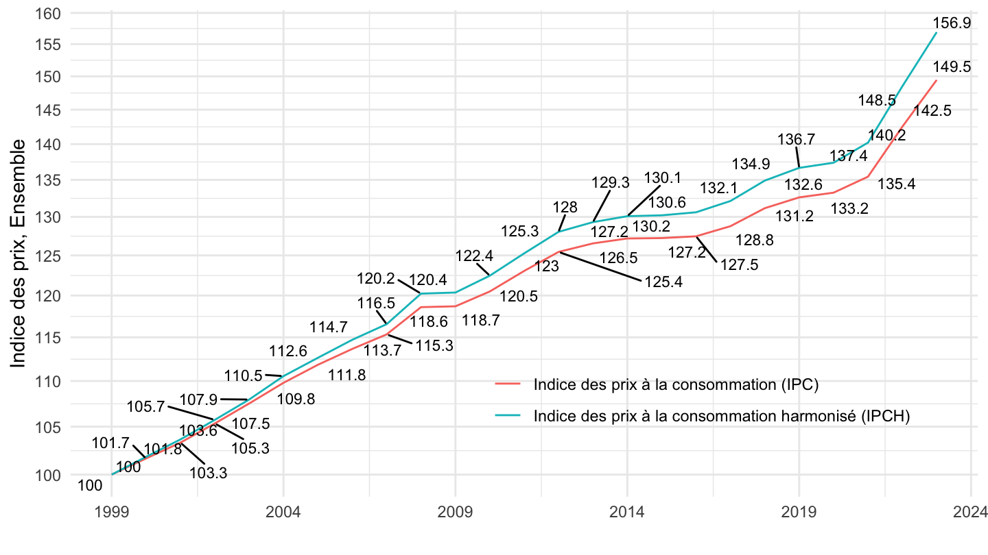
`IPCH-2015` |>
  bind_rows(`IPC-2015`) |>
  filter(COICOP2016 %in% c("00"),
         NATURE == "INDICE",
         REF_AREA == "FM",
         FREQ == "A",
         is.na(MENAGES_IPC) | MENAGES_IPC == "ENSEMBLE",
         is.na(PRIX_CONSO) | PRIX_CONSO == "SO") |>
  year_to_date() |>
  filter(date >= as.Date("1996-01-01")) |>

  group_by(INDICATEUR) |>
  arrange(date) |>
  mutate(OBS_VALUE = 100*OBS_VALUE/OBS_VALUE[date == as.Date("1996-01-01")]) |>
  ggplot() + ylab("Indice des prix, Ensemble") + xlab("") + theme_minimal() +
  geom_line(aes(x = date, y = OBS_VALUE, color = INDICATEUR)) +
  theme(legend.position = c(0.7, 0.2),
        legend.title = element_blank()) +
  scale_x_date(breaks = seq(1920, 2100, 2) |> paste0("-01-01") |> as.Date(),
               labels = date_format("%Y")) +
  scale_y_log10(breaks = seq(10, 300, 5),
                     labels = dollar_format(accuracy = 1, prefix = "")) +
  geom_text_repel(aes(x = date, y = OBS_VALUE, label = round(OBS_VALUE, 1)),
                  fontface ="plain", color = "black", size = 3)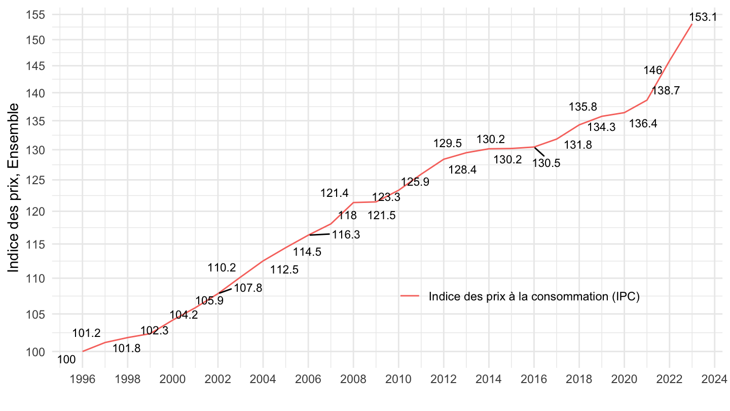
`IPCH-2015` |>
  bind_rows(`IPC-2015`) |>
  filter(COICOP2016 %in% c("00", "SO"),
         NATURE == "INDICE",
         REF_AREA == "FE",
         FREQ == "A",
         is.na(MENAGES_IPC) | MENAGES_IPC == "ENSEMBLE",
         is.na(PRIX_CONSO) | PRIX_CONSO == "SO" | PRIX_CONSO == "4018") |>
  year_to_date() |>
  filter(date >= as.Date("1996-01-01")) |>


  group_by(INDICATEUR) |>
  arrange(date) |>
  mutate(OBS_VALUE = 100*OBS_VALUE/OBS_VALUE[date == as.Date("1996-01-01")]) |>
  ggplot() + ylab("Indice des prix, Ensemble") + xlab("") + theme_minimal() +
  geom_line(aes(x = date, y = OBS_VALUE, color = INDICATEUR, linetype = COICOP2016)) +
  theme(legend.position = c(0.7, 0.2),
        legend.title = element_blank()) +
  scale_x_date(breaks = seq(1920, 2100, 2) |> paste0("-01-01") |> as.Date(),
               labels = date_format("%Y")) +
  scale_y_log10(breaks = seq(10, 300, 5),
                     labels = dollar_format(accuracy = 1, prefix = "")) +
  geom_text_repel(aes(x = date, y = OBS_VALUE, label = round(OBS_VALUE, 1)),
                  fontface ="plain", color = "black", size = 3)
`IPCH-2015` |>
  bind_rows(`IPC-2015`) |>
  filter(COICOP2016 %in% c("00"),
         NATURE == "INDICE",
         REF_AREA == "FM",
         FREQ == "A",
         is.na(MENAGES_IPC) | MENAGES_IPC == "ENSEMBLE",
         is.na(PRIX_CONSO) | PRIX_CONSO == "SO" | PRIX_CONSO == "4018") |>
  year_to_date() |>
  filter(date >= as.Date("1996-01-01")) |>

  group_by(INDICATEUR) |>
  arrange(date) |>
  mutate(OBS_VALUE = 100*OBS_VALUE/OBS_VALUE[date == as.Date("1996-01-01")]) |>
  ggplot() + ylab("Indice des prix, Ensemble") + xlab("") + theme_minimal() +
  geom_line(aes(x = date, y = OBS_VALUE, color = INDICATEUR)) +
  theme(legend.position = c(0.7, 0.2),
        legend.title = element_blank()) +
  scale_x_date(breaks = seq(1920, 2100, 2) |> paste0("-01-01") |> as.Date(),
               labels = date_format("%Y")) +
  scale_y_log10(breaks = seq(10, 300, 5),
                     labels = dollar_format(accuracy = 1, prefix = "")) +
  geom_text_repel(aes(x = date, y = OBS_VALUE, label = round(OBS_VALUE, 1)),
                  fontface ="plain", color = "black", size = 3)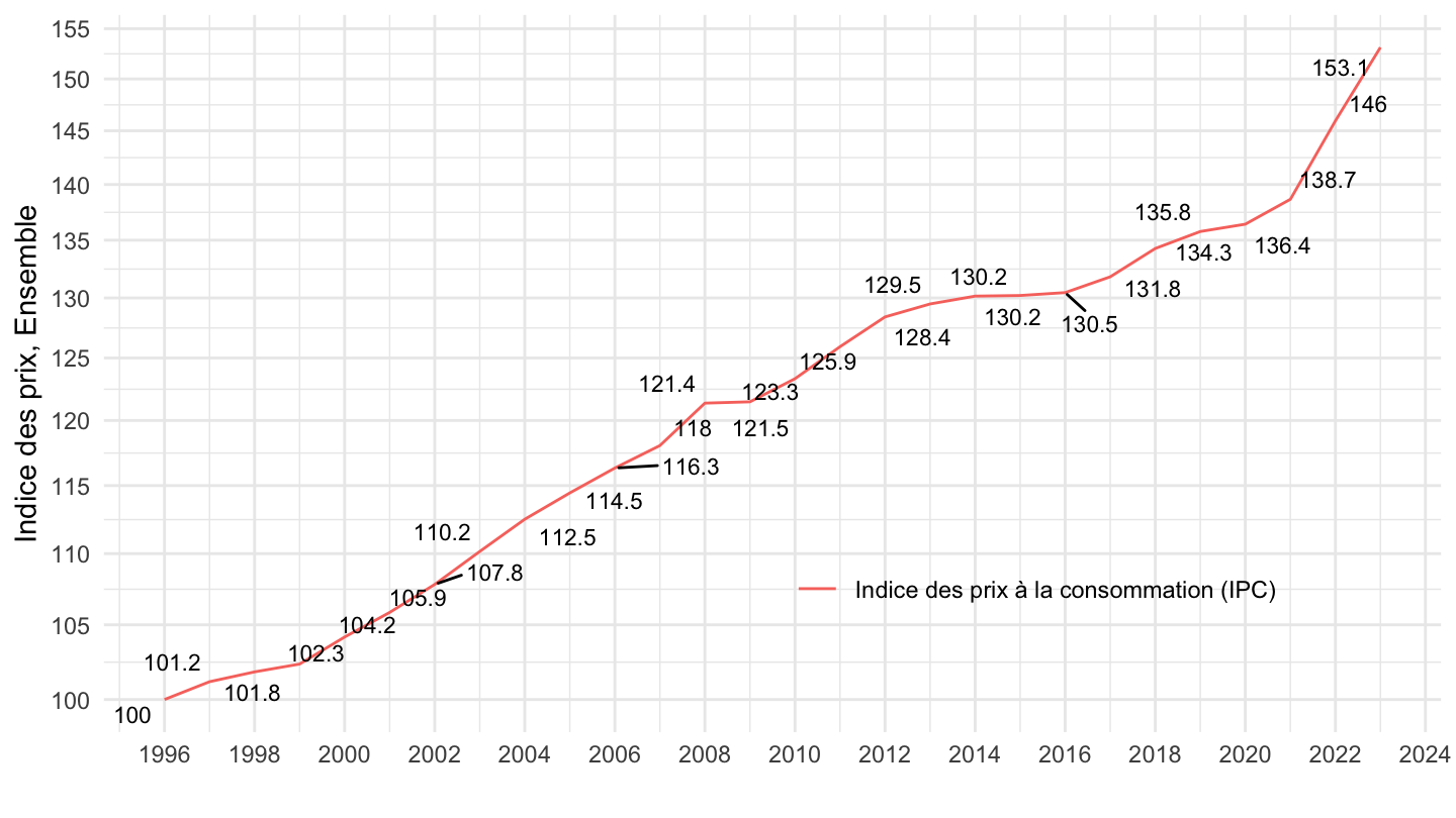
`IPCH-2015` |>
  bind_rows(`IPC-2015`) |>
  filter(COICOP2016 %in% c("00"),
         NATURE == "INDICE",
         REF_AREA == "FE",
         FREQ == "A",
         is.na(MENAGES_IPC) | MENAGES_IPC == "ENSEMBLE",
         is.na(PRIX_CONSO) | PRIX_CONSO == "SO") |>
  year_to_date() |>
  filter(date >= as.Date("1996-01-01")) |>

  group_by(INDICATEUR) |>
  arrange(date) |>
  mutate(OBS_VALUE = 100*OBS_VALUE/OBS_VALUE[date == as.Date("1996-01-01")],
         OBS_VALUE = OBS_VALUE/lag(OBS_VALUE)-1) |>
  ggplot() + ylab("Indice des prix, Ensemble") + xlab("") + theme_minimal() +
  geom_line(aes(x = date, y = OBS_VALUE, color = INDICATEUR)) +
  #
  theme(legend.position = c(0.3, 0.8),
        legend.title = element_blank()) +
  scale_x_date(breaks = seq(1920, 2100, 2) |> paste0("-01-01") |> as.Date(),
               labels = date_format("%Y")) +
  scale_y_continuous(breaks = 0.01*seq(-10, 10, 1),
                     labels = percent_format())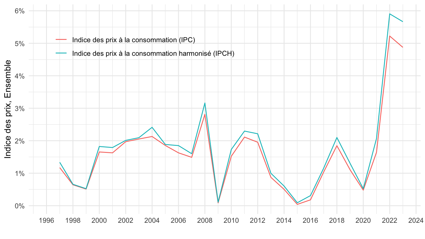
`IPCH-2015` |>
  bind_rows(`IPC-2015`) |>
  filter(COICOP2016 %in% c("00"),
         NATURE == "INDICE",
         REF_AREA == "FE",
         FREQ == "M",
         is.na(MENAGES_IPC) | MENAGES_IPC == "ENSEMBLE",
         is.na(PRIX_CONSO) | PRIX_CONSO == "SO") |>
  month_to_date() |>

  group_by(INDICATEUR) |>
  arrange(date) |>
  mutate(OBS_VALUE = 100*OBS_VALUE/OBS_VALUE[date == as.Date("1996-01-01")]) |>
  ggplot() + ylab("Indice des prix, Ensemble") + xlab("") + theme_minimal() +
  geom_line(aes(x = date, y = OBS_VALUE, color = INDICATEUR)) +

  theme(legend.position = c(0.7, 0.2),
        legend.title = element_blank()) +
  scale_x_date(breaks = seq(1920, 2100, 5) |> paste0("-01-01") |> as.Date(),
               labels = date_format("%Y")) +
  scale_y_log10(breaks = seq(10, 300, 5),
                     labels = dollar_format(accuracy = 1, prefix = ""))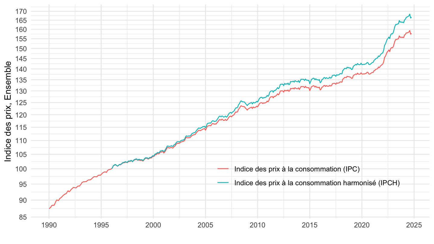
`IPCH-2015` |>
  bind_rows(`IPC-2015`) |>
  filter(COICOP2016 %in% c("00"),
         NATURE == "INDICE",
         REF_AREA == "FE",
         FREQ == "A",
         is.na(MENAGES_IPC) | MENAGES_IPC == "ENSEMBLE",
         is.na(PRIX_CONSO) | PRIX_CONSO == "SO") |>
  year_to_date() |>

  group_by(INDICATEUR) |>
  arrange(date) |>
  mutate(OBS_VALUE = 100*OBS_VALUE/OBS_VALUE[date == as.Date("1996-01-01")]) |>
  ungroup() |>
  mutate(OBS_VALUE = 100*OBS_VALUE/OBS_VALUE[date == as.Date("1990-01-01")]) |>

  ggplot() + ylab("Indice des prix, Ensemble") + xlab("") + theme_minimal() +
  geom_line(aes(x = date, y = OBS_VALUE, color = INDICATEUR)) +

  theme(legend.position = c(0.7, 0.2),
        legend.title = element_blank()) +
  scale_x_date(breaks = seq(1920, 2100, 5) |> paste0("-01-01") |> as.Date(),
               labels = date_format("%Y")) +
  scale_y_log10(breaks = seq(10, 300, 5),
                     labels = dollar_format(accuracy = 1, prefix = ""))
invisible(Sys.setlocale("LC_TIME", "fr_CA.UTF-8"))
`IPCH-2015` |>
  bind_rows(`IPC-2015`) |>
  filter(COICOP2016 %in% c("00"),
         NATURE == "INDICE",
         REF_AREA == "FE",
         FREQ == "M",
         is.na(MENAGES_IPC) | MENAGES_IPC == "ENSEMBLE",
         is.na(PRIX_CONSO) | PRIX_CONSO == "SO") |>
  month_to_date() |>

  group_by(INDICATEUR) |>
  arrange(date) |>
  mutate(OBS_VALUE = OBS_VALUE/lag(OBS_VALUE, 12)-1) |>
  filter(date >= Sys.Date() - years(3)) |>
  select(date, OBS_VALUE, Indicateur) |>
  na.omit() |>
  ggplot() + ylab("Inflation sur un an (IPC, IPCH)") + xlab("") + theme_minimal() +
  geom_line(aes(x = date, y = OBS_VALUE, color = Indicateur)) +

  scale_x_date(breaks = "2 months",
               labels = date_format("%b %Y")) +
  theme(legend.position = c(0.5, 0.2),
        legend.title = element_blank(),
        axis.text.x = element_text(angle = 45, vjust = 1, hjust = 1)) +
  scale_y_continuous(breaks = 0.01*seq(-100, 300, 0.5),
                     labels = percent_format(accuracy = .1, prefix = "")) +
  geom_text_repel(aes(x = date, y = OBS_VALUE, label = percent(OBS_VALUE, acc = 0.1)),
                  fontface ="plain", color = "black", size = 3)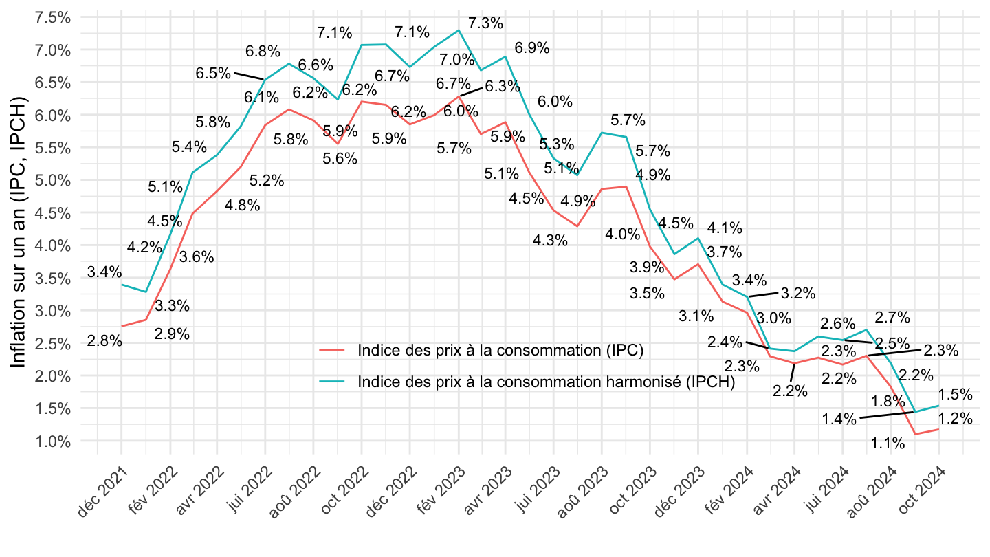
`IPCH-2015` |>
  bind_rows(`IPC-2015`) |>
  filter(COICOP2016 %in% c("00"),
         NATURE == "INDICE",
         REF_AREA == "FE",
         FREQ == "M",
         is.na(MENAGES_IPC) | MENAGES_IPC == "ENSEMBLE",
         is.na(PRIX_CONSO) | PRIX_CONSO == "SO") |>
  month_to_date() |>

  group_by(INDICATEUR) |>
  arrange(date) |>
  mutate(OBS_VALUE = OBS_VALUE/lag(OBS_VALUE, 12)-1) |>
  filter(date >= Sys.Date() - years(2)) |>
  select(date, OBS_VALUE, INDICATEUR) |>
  na.omit() |>
  ggplot() + ylab("Inflation sur un an (IPC, IPCH)") + xlab("") + theme_minimal() +
  geom_line(aes(x = date, y = OBS_VALUE, color = INDICATEUR)) +

  scale_x_date(breaks = "1 month",
               labels = date_format("%b %Y")) +
  theme(legend.position = c(0.65, 0.2),
        legend.title = element_blank(),
        axis.text.x = element_text(angle = 45, vjust = 1, hjust = 1)) +
  scale_y_continuous(breaks = 0.01*seq(-100, 300, 0.5),
                     labels = percent_format(accuracy = .1, prefix = "")) +
  geom_text_repel(aes(x = date, y = OBS_VALUE, label = percent(OBS_VALUE, acc = 0.1)),
                  fontface ="plain", color = "black", size = 3)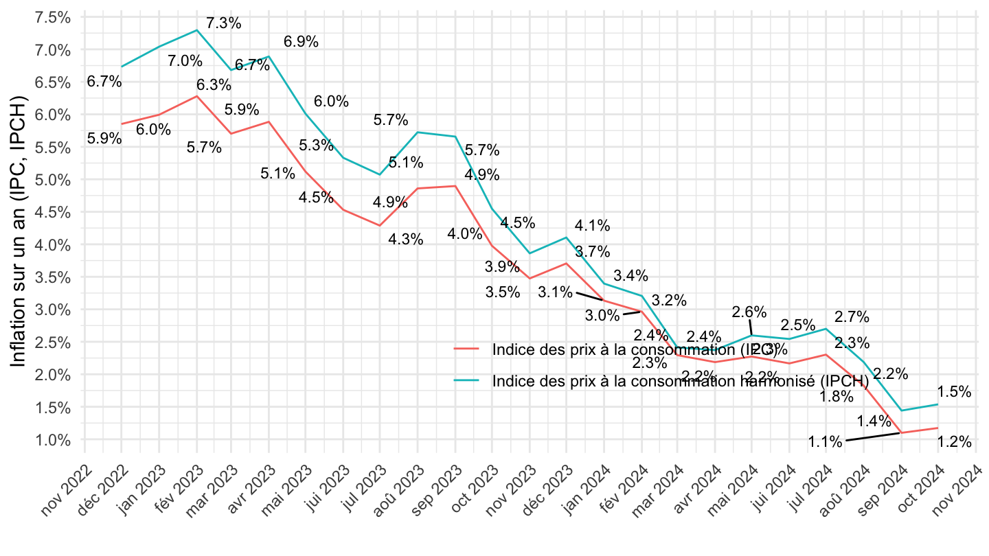
`IPCH-2015` |>
  bind_rows(`IPC-2015`) |>
  filter(COICOP2016 %in% c("00"),
         NATURE == "INDICE",
         REF_AREA == "FE",
         FREQ == "M",
         is.na(MENAGES_IPC) | MENAGES_IPC == "ENSEMBLE",
         is.na(PRIX_CONSO) | PRIX_CONSO == "SO") |>
  month_to_date() |>

  group_by(INDICATEUR) |>
  filter(date >= as.Date("2021-01-01")) |>
  arrange(date) |>
  mutate(OBS_VALUE = OBS_VALUE/lag(OBS_VALUE, 12)-1) |>
  select(date, OBS_VALUE, INDICATEUR) |>
  na.omit() |>
  ggplot() + ylab("Inflation sur un an (IPC, IPCH)") + xlab("") + theme_minimal() +
  geom_line(aes(x = date, y = OBS_VALUE, color = INDICATEUR)) +

  scale_x_date(breaks = "1 month",
               labels = date_format("%b %Y")) +
  theme(legend.position = c(0.65, 0.2),
        legend.title = element_blank(),
        axis.text.x = element_text(angle = 45, vjust = 1, hjust = 1)) +
  scale_y_continuous(breaks = 0.01*seq(-100, 300, 0.5),
                     labels = percent_format(accuracy = .1, prefix = "")) +
  geom_text_repel(aes(x = date, y = OBS_VALUE, label = percent(OBS_VALUE, acc = 0.1)),
                  fontface ="plain", color = "black", size = 3)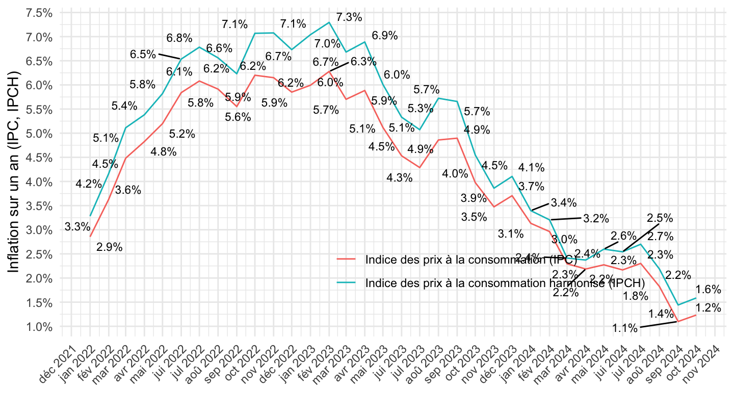
`IPCH-2015` |>
  bind_rows(`IPC-2015`) |>
  filter(COICOP2016 %in% c("00"),
         NATURE == "INDICE",
         REF_AREA == "FE",
         FREQ == "M",
         is.na(MENAGES_IPC) | MENAGES_IPC == "ENSEMBLE",
         is.na(PRIX_CONSO) | PRIX_CONSO == "SO") |>
  month_to_date() |>

  group_by(INDICATEUR) |>
  filter(date >= as.Date("2011-01-01")) |>
  arrange(date) |>
  mutate(OBS_VALUE = OBS_VALUE/lag(OBS_VALUE, 12)-1) |>
  select(date, OBS_VALUE, INDICATEUR) |>
  na.omit() |>
  ggplot() + ylab("Inflation sur un an (IPC, IPCH)") + xlab("") + theme_minimal() +
  geom_line(aes(x = date, y = OBS_VALUE, color = INDICATEUR)) +

  scale_x_date(breaks = seq(1920, 2100, 2) |> paste0("-01-01") |> as.Date(),
               labels = date_format("%Y")) +
  theme(legend.position = c(0.35, 0.9),
        legend.title = element_blank()) +
  scale_y_continuous(breaks = 0.01*seq(-100, 300, 0.5),
                     labels = percent_format(accuracy = .1, prefix = ""))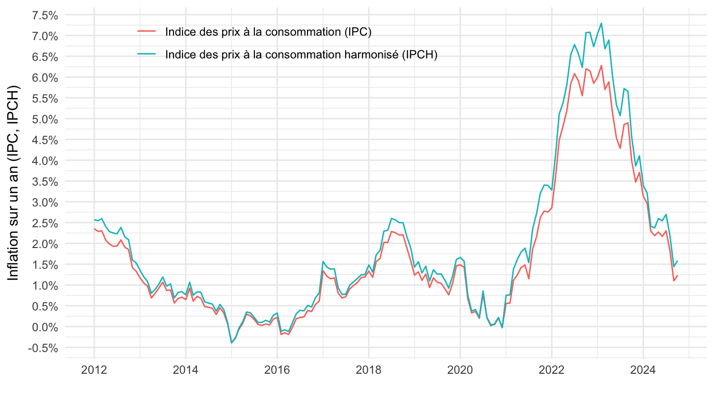
`IPCH-2015` |>
  bind_rows(`IPC-2015`) |>
  filter(COICOP2016 %in% c("00"),
         NATURE == "INDICE",
         REF_AREA == "FE",
         FREQ == "M",
         is.na(MENAGES_IPC) | MENAGES_IPC == "ENSEMBLE",
         is.na(PRIX_CONSO) | PRIX_CONSO == "SO") |>
  month_to_date() |>

  group_by(INDICATEUR) |>
  filter(date >= as.Date("1996-01-01")) |>
  arrange(date) |>
  mutate(OBS_VALUE = OBS_VALUE/lag(OBS_VALUE, 12)-1) |>
  ggplot() + ylab("Inflation sur un an (IPC, IPCH)") + xlab("") + theme_minimal() +
  geom_line(aes(x = date, y = OBS_VALUE, color = INDICATEUR)) +

  scale_x_date(breaks = seq(1920, 2100, 2) |> paste0("-01-01") |> as.Date(),
               labels = date_format("%Y")) +
  theme(legend.position = c(0.35, 0.9),
        legend.title = element_blank()) +
  scale_y_continuous(breaks = 0.01*seq(-100, 300, 0.5),
                     labels = percent_format(accuracy = .1, prefix = ""))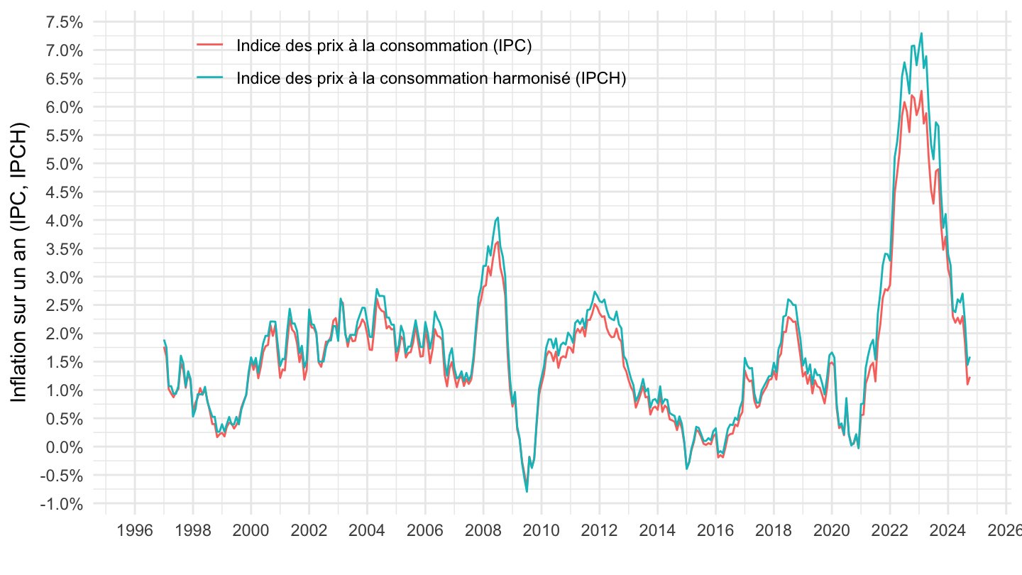
`IPCH-2015` |>
  bind_rows(`IPC-2015`) |>
  filter(COICOP2016 %in% c("00"),
         NATURE == "INDICE",
         REF_AREA == "FE",
         FREQ == "M",
         is.na(MENAGES_IPC) | MENAGES_IPC == "ENSEMBLE",
         is.na(PRIX_CONSO) | PRIX_CONSO == "SO") |>
  month_to_date() |>

  group_by(INDICATEUR) |>
  filter(date >= as.Date("1990-01-01")) |>
  arrange(date) |>
  mutate(OBS_VALUE = OBS_VALUE/lag(OBS_VALUE, 12)-1) |>
  ggplot() + ylab("Inflation sur un an (IPC, IPCH)") + xlab("") + theme_minimal() +
  geom_line(aes(x = date, y = OBS_VALUE, color = INDICATEUR)) +

  scale_x_date(breaks = seq(1920, 2100, 2) |> paste0("-01-01") |> as.Date(),
               labels = date_format("%Y")) +
  theme(legend.position = c(0.25, 0.9),
        legend.title = element_blank()) +
  scale_y_continuous(breaks = 0.01*seq(-100, 300, 0.5),
                     labels = percent_format(accuracy = .1, prefix = ""))
`IPCH-2015` |>
  bind_rows(`IPC-2015`) |>
  filter(COICOP2016 %in% c("00"),
         NATURE == "INDICE",
         REF_AREA == "FE",
         FREQ == "M",
         is.na(MENAGES_IPC) | MENAGES_IPC == "ENSEMBLE",
         is.na(PRIX_CONSO) | PRIX_CONSO == "SO") |>
  month_to_date() |>

  group_by(INDICATEUR) |>
  filter(date >= as.Date("1996-01-01")) |>
  arrange(date) |>
  mutate(OBS_VALUE = (OBS_VALUE/lag(OBS_VALUE, 24))^(1/2)-1) |>
  ggplot() + ylab("Inflation annuelle sur 2 ans (IPC, IPCH)") + xlab("") + theme_minimal() +
  geom_line(aes(x = date, y = OBS_VALUE, color = INDICATEUR)) +

  scale_x_date(breaks = seq(1920, 2100, 2) |> paste0("-01-01") |> as.Date(),
               labels = date_format("%Y")) +
  theme(legend.position = c(0.3, 0.8),
        legend.title = element_blank()) +
  scale_y_continuous(breaks = 0.01*seq(-100, 300, 0.5),
                     labels = percent_format(accuracy = .1, prefix = ""))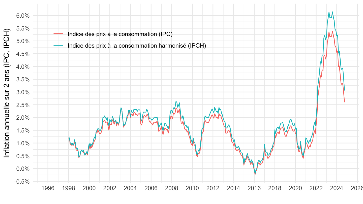
`IPCH-2015` |>
  bind_rows(`IPC-2015`) |>
  filter(COICOP2016 %in% c("00"),
         NATURE == "INDICE",
         REF_AREA == "FE",
         FREQ == "M",
         is.na(MENAGES_IPC) | MENAGES_IPC == "ENSEMBLE",
         is.na(PRIX_CONSO) | PRIX_CONSO == "SO") |>
  month_to_date() |>

  group_by(INDICATEUR) |>
  filter(date >= as.Date("1996-01-01")) |>
  arrange(date) |>
  mutate(OBS_VALUE = (OBS_VALUE/lag(OBS_VALUE, 24))-1) |>
  ggplot() + ylab("Inflation annuelle sur 2 ans (IPC, IPCH)") + xlab("") + theme_minimal() +
  geom_line(aes(x = date, y = OBS_VALUE, color = INDICATEUR)) +

  scale_x_date(breaks = seq(1920, 2100, 2) |> paste0("-01-01") |> as.Date(),
               labels = date_format("%Y")) +
  theme(legend.position = c(0.3, 0.8),
        legend.title = element_blank()) +
  scale_y_continuous(breaks = 0.01*seq(-100, 300, 1),
                     labels = percent_format(accuracy = .1, prefix = ""))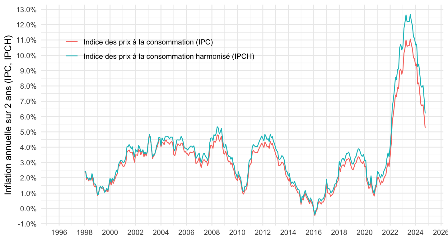
`IPCH-2015` |>
  bind_rows(`IPC-2015`) |>
  filter(COICOP2016 %in% c("00"),
         NATURE == "INDICE",
         REF_AREA == "FE",
         FREQ == "M",
         is.na(MENAGES_IPC) | MENAGES_IPC == "ENSEMBLE",
         is.na(PRIX_CONSO) | PRIX_CONSO == "SO") |>
  month_to_date() |>

  group_by(INDICATEUR) |>
  arrange(date) |>
  mutate(OBS_VALUE = (OBS_VALUE/lag(OBS_VALUE, 24))-1) |>
  filter(date >= as.Date("2021-01-01")) |>
  ggplot() + ylab("Inflation sur 2 ans (IPC, IPCH)") + xlab("") + theme_minimal() +
  geom_line(aes(x = date, y = OBS_VALUE, color = INDICATEUR)) +
  scale_x_date(breaks = seq(1920, 2100, 1) |> paste0("-01-01") |> as.Date(),
               labels = date_format("%Y")) +
  theme(legend.position = c(0.28, 0.9),
        legend.title = element_blank()) +
  scale_y_continuous(breaks = 0.01*seq(-100, 300, 1),
                     labels = percent_format(accuracy = .1, prefix = "")) +
  geom_text(data = . %>%
              filter(month(date) %in% c(1, 4, 7, 10)), aes(x = date, y = OBS_VALUE, label = percent(OBS_VALUE, acc = 0.1)))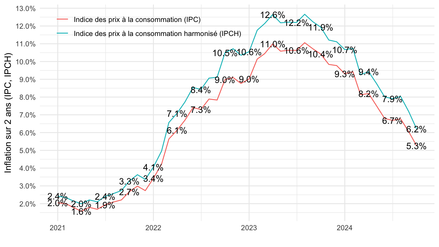
`IPCH-2015` |>
  bind_rows(`IPC-2015`) |>
  filter(COICOP2016 %in% c("00"),
         NATURE == "INDICE",
         REF_AREA == "FE",
         FREQ == "M",
         is.na(MENAGES_IPC) | MENAGES_IPC == "ENSEMBLE",
         is.na(PRIX_CONSO) | PRIX_CONSO == "SO") |>
  month_to_date() |>

  group_by(INDICATEUR) |>
  arrange(date) |>
  mutate(OBS_VALUE = (OBS_VALUE/lag(OBS_VALUE, 36))-1) |>
  filter(date >= as.Date("2021-01-01")) |>
  ggplot() + ylab("Inflation sur 3 ans (IPC, IPCH)") + xlab("") + theme_minimal() +
  geom_line(aes(x = date, y = OBS_VALUE, color = INDICATEUR)) +
  scale_x_date(breaks = seq(1920, 2100, 1) |> paste0("-01-01") |> as.Date(),
               labels = date_format("%Y")) +
  theme(legend.position = c(0.28, 0.9),
        legend.title = element_blank()) +
  scale_y_continuous(breaks = 0.01*seq(-100, 300, 1),
                     labels = percent_format(accuracy = .1, prefix = "")) +
  geom_text(data = . %>%
              filter(month(date) %in% c(1, 4, 7, 10)), aes(x = date, y = OBS_VALUE, label = percent(OBS_VALUE, acc = 0.1)))
`IPCH-2015` |>
  filter(INDICATEUR == "IPCH",
         COICOP2016 %in% c("041", "00"),
         FREQ == "M",
         NATURE == "INDICE") |>
  month_to_date() |>

  group_by(COICOP2016) |>
  mutate(OBS_VALUE = 100*OBS_VALUE/OBS_VALUE[date == as.Date("1996-01-01")]) |>
  ggplot() + ylab("Indice des prix") + xlab("") + theme_minimal() +
  geom_line(aes(x = date, y = OBS_VALUE, color = COICOP2016)) +

  scale_x_date(breaks = seq(1920, 2100, 2) |> paste0("-01-01") |> as.Date(),
               labels = date_format("%Y")) +
  theme(legend.position = c(0.75, 0.3),
        legend.title = element_blank()) +
  scale_y_log10(breaks = seq(0, 200, 10),
                     labels = dollar_format(accuracy = 1, prefix = ""))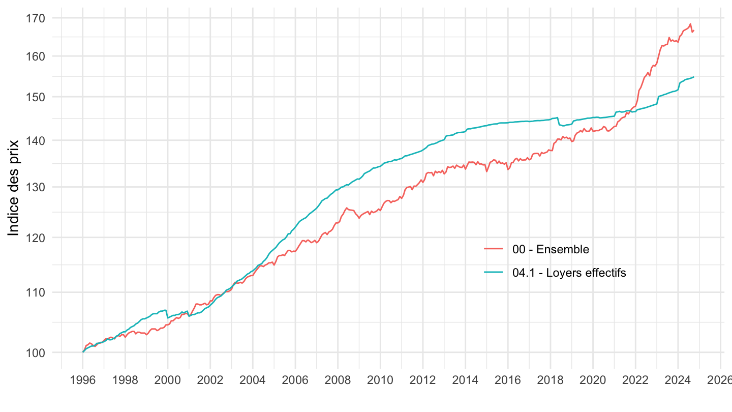
`IPCH-2015` |>
  filter(INDICATEUR == "IPCH",
         COICOP2016 %in% c("041", "00"),
         FREQ == "M",
         NATURE == "INDICE") |>
  month_to_date() |>

  group_by(COICOP2016) |>
  filter(date >= as.Date("1999-01-01")) |>
  mutate(OBS_VALUE = 100*OBS_VALUE/OBS_VALUE[date == as.Date("1999-01-01")]) |>
  ggplot() + ylab("Indice des prix") + xlab("") + theme_minimal() +
  geom_line(aes(x = date, y = OBS_VALUE, color = COICOP2016)) +

  scale_x_date(breaks = seq(1920, 2100, 5) |> paste0("-01-01") |> as.Date(),
               labels = date_format("%Y")) +
  theme(legend.position = c(0.75, 0.3),
        legend.title = element_blank()) +
  scale_y_log10(breaks = seq(0, 200, 5),
                     labels = dollar_format(accuracy = 1, prefix = ""))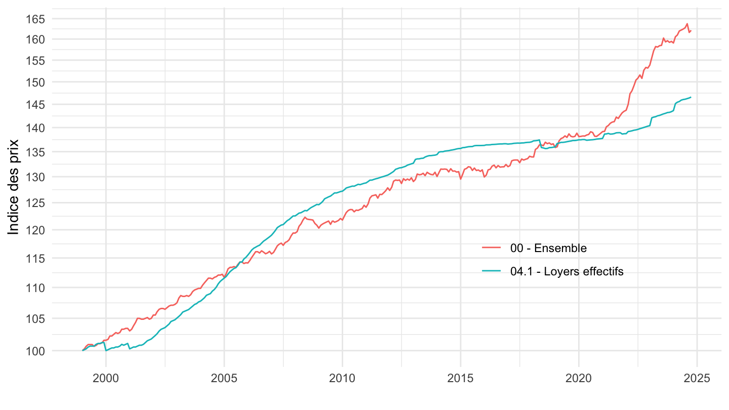
`IPCH-2015` |>
  filter(INDICATEUR == "IPCH",
         COICOP2016 %in% c("041", "00"),
         FREQ == "M",
         NATURE == "INDICE") |>
  month_to_date() |>

  filter(date >= max(date) - years(2)) |>
  group_by(COICOP2016) |>
  arrange(date) |>
  mutate(OBS_VALUE = 100*OBS_VALUE/OBS_VALUE[1]) |>
  ggplot() + ylab("Indice des prix") + xlab("") + theme_minimal() +
  geom_line(aes(x = date, y = OBS_VALUE, color = COICOP2016)) +
  theme_minimal() + xlab("") + ylab("") +
  scale_x_date(breaks = "1 month",
               labels = date_format("%b %Y")) +
  theme(legend.position = c(0.28, 0.87),
        legend.title = element_blank(),
        axis.text.x = element_text(angle = 45, vjust = 0.5, hjust=1)) +
  scale_y_log10(breaks = seq(0, 200, 2),
                     labels = dollar_format(accuracy = 1, prefix = "")) +
  geom_text_repel(aes(x = date, y = OBS_VALUE, label = round(OBS_VALUE, 1)),
                  fontface ="plain", color = "black", size = 3)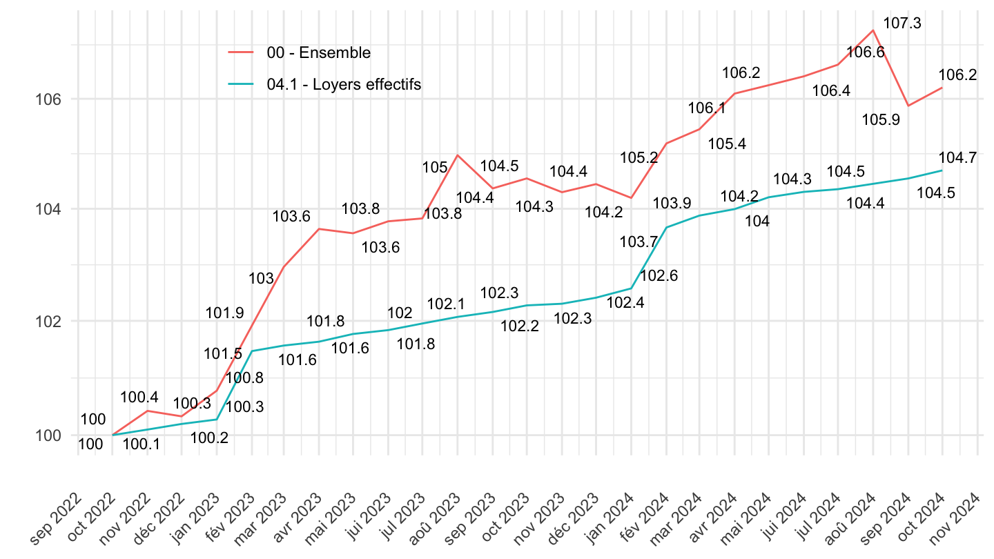
`IPCH-2015` |>
  filter(INDICATEUR == "IPCH",
         COICOP2016 %in% c( "00", "01", "022"),
         FREQ == "M",
         NATURE == "INDICE") |>
  month_to_date() |>

  filter(date >= as.Date("2021-01-01")) |>
  group_by(COICOP2016) |>
  arrange(date) |>
  mutate(OBS_VALUE = 100*OBS_VALUE/OBS_VALUE[1]) |>
  ggplot() + ylab("Indice des prix") + xlab("") + theme_minimal() +
  geom_line(aes(x = date, y = OBS_VALUE, color = COICOP2016)) +
  theme_minimal() + xlab("") + ylab("") +
  scale_x_date(breaks = "2 months",
               labels = date_format("%b %Y")) +
  theme(legend.position = c(0.28, 0.87),
        legend.title = element_blank(),
        axis.text.x = element_text(angle = 45, vjust = 0.5, hjust=1)) +
  scale_y_log10(breaks = seq(0, 200, 2),
                     labels = dollar_format(accuracy = 1, prefix = "")) +
  geom_label(data = . %>% filter(date == max(date)),
                  aes(x = date, y = OBS_VALUE, label = round(OBS_VALUE, 1), color = COICOP2016),
                  fontface ="plain", size = 3)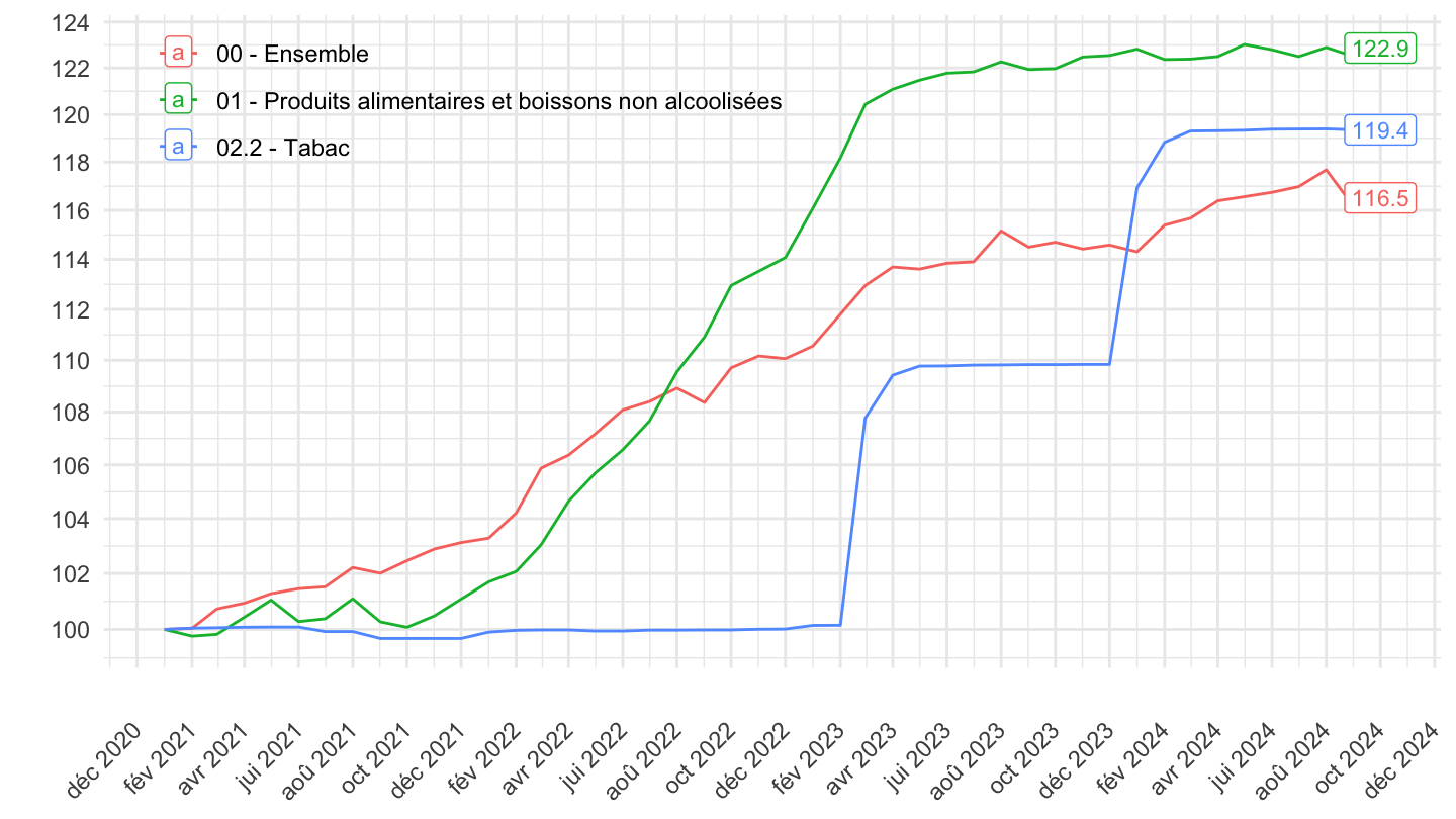
`IPCH-2015` |>
  filter(INDICATEUR == "IPCH",
         COICOP2016 %in% c( "00", "01"),
         FREQ == "M",
         NATURE == "INDICE") |>
  month_to_date() |>

  filter(date >= as.Date("2021-01-01")) |>
  group_by(COICOP2016) |>
  arrange(date) |>
  mutate(OBS_VALUE = 100*OBS_VALUE/OBS_VALUE[1]) |>
  ggplot() + ylab("Indice des prix") + xlab("") + theme_minimal() +
  geom_line(aes(x = date, y = OBS_VALUE, color = COICOP2016)) +
  theme_minimal() + xlab("") + ylab("100 = Janvier 2021") +
  scale_x_date(breaks = "2 months",
               labels = date_format("%b %Y")) +
  theme(legend.position = c(0.28, 0.87),
        legend.title = element_blank(),
        axis.text.x = element_text(angle = 45, vjust = 0.5, hjust=1)) +
  scale_y_log10(breaks = seq(0, 200, 2),
                     labels = dollar_format(accuracy = 1, prefix = "")) +
  geom_label(data = . %>% filter(date == max(date)),
                  aes(x = date, y = OBS_VALUE, label = round(OBS_VALUE, 1), color = COICOP2016),
                  fontface ="plain", size = 3)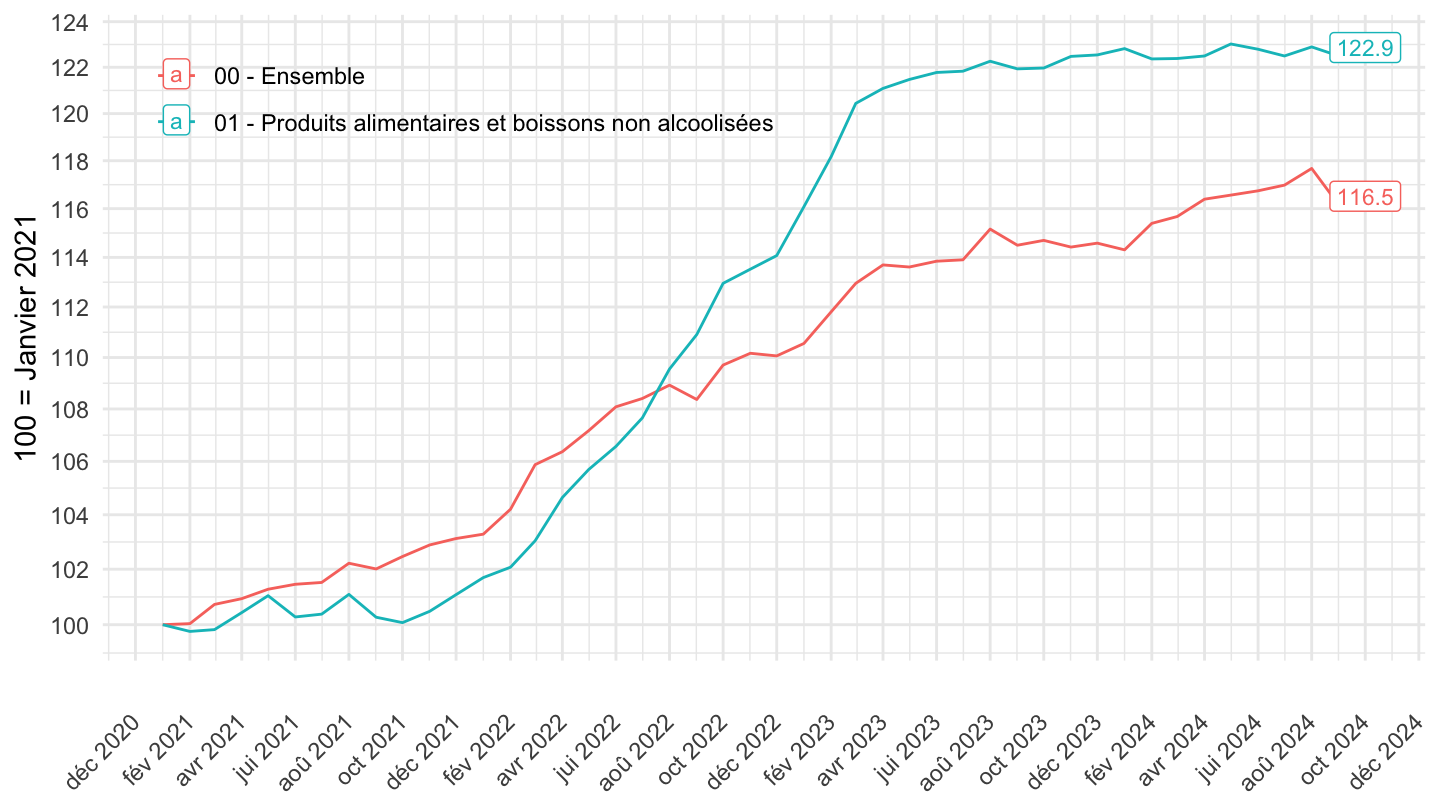
`IPCH-2015` |>
  filter(INDICATEUR == "IPCH",
         COICOP2016 %in% c("041", "00", "01", "045"),
         FREQ == "M",
         NATURE == "INDICE") |>
  month_to_date() |>

  filter(date >= as.Date("2021-01-01")) |>
  group_by(COICOP2016) |>
  arrange(date) |>
  mutate(OBS_VALUE = 100*OBS_VALUE/OBS_VALUE[1]) |>
  ggplot() + ylab("Indice des prix") + xlab("") + theme_minimal() +
  geom_line(aes(x = date, y = OBS_VALUE, color = Coicop2016)) +
  theme_minimal() + xlab("") + ylab("") +
  scale_x_date(breaks = "2 months",
               labels = date_format("%b %Y")) +
  theme(legend.position = c(0.28, 0.87),
        legend.title = element_blank(),
        axis.text.x = element_text(angle = 45, vjust = 0.5, hjust=1)) +
  scale_y_log10(breaks = seq(0, 200, 2),
                     labels = dollar_format(accuracy = 1, prefix = "")) +
  geom_text_repel(data = . %>% filter(date == max(date)),
                  aes(x = date, y = OBS_VALUE, label = round(OBS_VALUE, 1)),
                  fontface ="plain", color = "black", size = 3)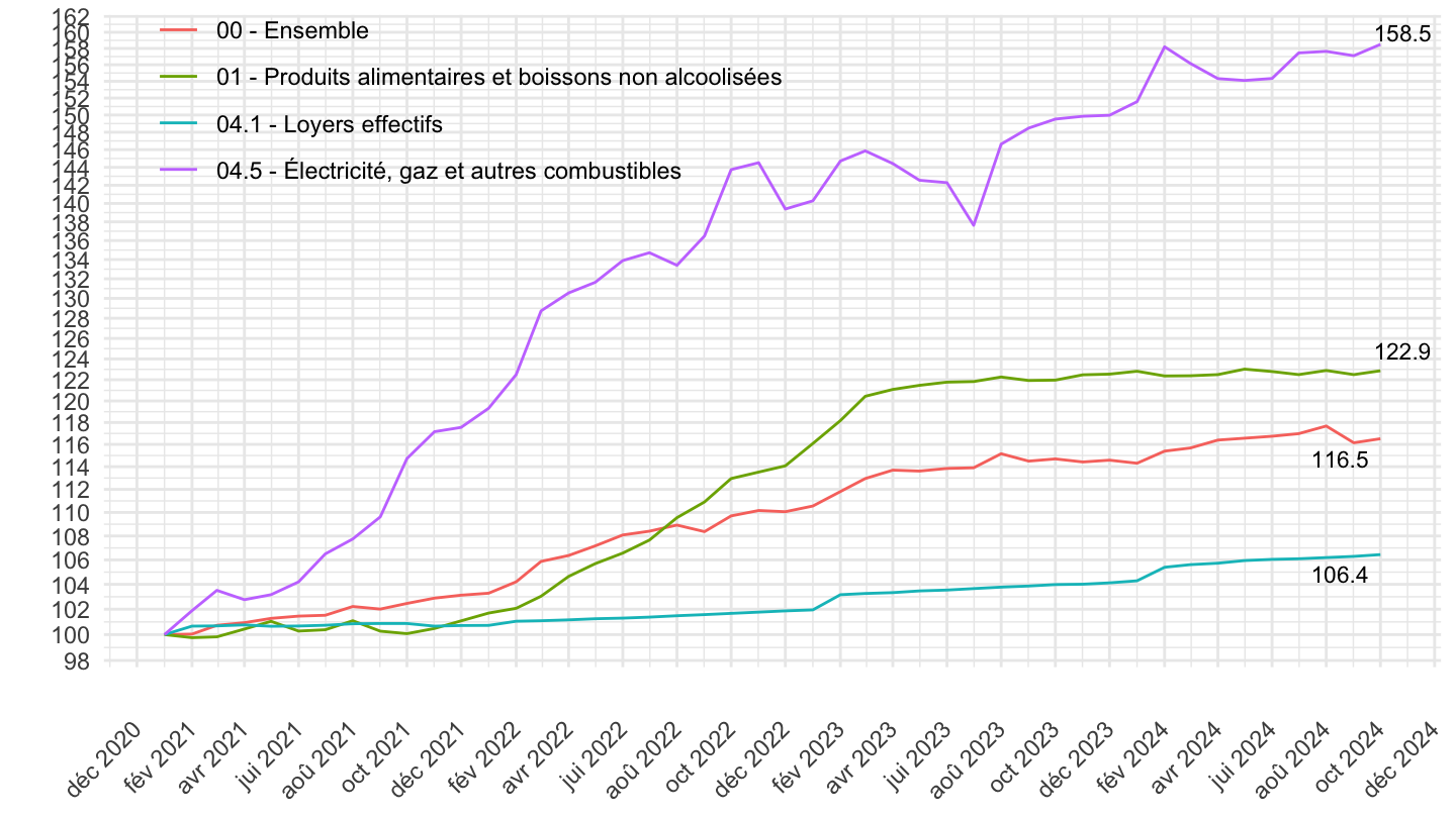
`IPC-2015` |>
  filter(INDICATEUR == "IPC",
         COICOP2016 %in% c("00", "01", "045"),
         FREQ == "M",
         NATURE == "INDICE",
         PRIX_CONSO == "SO",
         MENAGES_IPC == "ENSEMBLE",
         REF_AREA == "FE") |>
  month_to_date() |>
  arrange(date) |>

  filter(date >= as.Date("2019-07-01")) |>
  group_by(COICOP2016) |>
  arrange(date) |>
  mutate(OBS_VALUE = 100*OBS_VALUE/OBS_VALUE[1]) |>
  ggplot() + ylab("Indice des prix") + xlab("") + theme_minimal() +
  geom_line(aes(x = date, y = OBS_VALUE, color = Coicop2016)) +
  theme_minimal() + xlab("") + ylab("") +
  scale_x_date(breaks = "2 months",
               labels = date_format("%b %Y")) +
  theme(legend.position = c(0.28, 0.87),
        legend.title = element_blank(),
        axis.text.x = element_text(angle = 45, vjust = 0.5, hjust=1)) +
  scale_y_log10(breaks = seq(0, 200, 5),
                     labels = dollar_format(accuracy = 1, prefix = "")) +
  geom_label(data = . %>% filter(date == max(date)),
                  aes(x = date, y = OBS_VALUE, label = round(OBS_VALUE, 1), color = Coicop2016),
                  fontface ="plain", size = 3)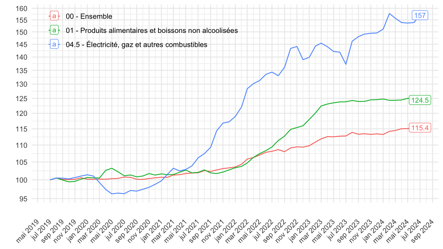
`IPCH-2015` |>
  filter(INDICATEUR == "IPCH",
         COICOP2016 %in% c("041", "00", "01", "045"),
         FREQ == "M",
         NATURE == "INDICE") |>
  month_to_date() |>

  filter(date >= max(date) - years(2)) |>
  group_by(COICOP2016) |>
  arrange(date) |>
  mutate(OBS_VALUE = 100*OBS_VALUE/OBS_VALUE[1]) |>
  ggplot() + ylab("Indice des prix") + xlab("") + theme_minimal() +
  geom_line(aes(x = date, y = OBS_VALUE, color = Coicop2016)) +
  theme_minimal() + xlab("") + ylab("") +
  scale_x_date(breaks = "1 month",
               labels = date_format("%b %Y")) +
  theme(legend.position = c(0.28, 0.87),
        legend.title = element_blank(),
        axis.text.x = element_text(angle = 45, vjust = 0.5, hjust=1)) +
  scale_y_log10(breaks = seq(0, 200, 2),
                     labels = dollar_format(accuracy = 1, prefix = "")) +
  geom_text_repel(aes(x = date, y = OBS_VALUE, label = round(OBS_VALUE, 1)),
                  fontface ="plain", color = "black", size = 3)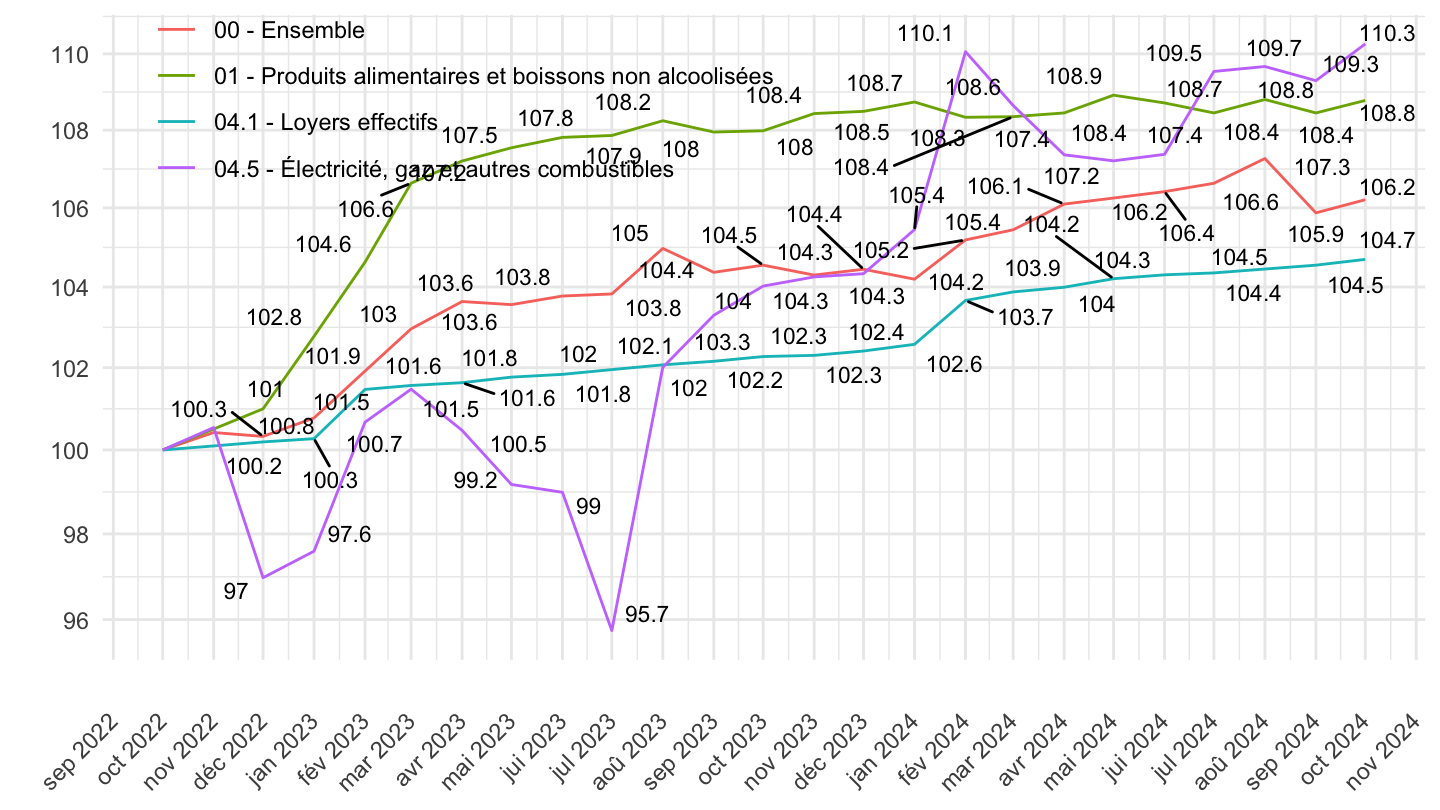
`IPCH-2015` |>
  filter(INDICATEUR == "IPCH",
         COICOP2016 %in% c("041", "00", "01", "045"),
         FREQ == "M",
         NATURE == "INDICE") |>
  month_to_date() |>

  filter(date >= as.Date("2017-01-01")) |>
  group_by(COICOP2016) |>
  arrange(date) |>
  mutate(OBS_VALUE = 100*OBS_VALUE/OBS_VALUE[1]) |>
  ggplot() + ylab("Indice des prix") + xlab("") + theme_minimal() +
  geom_line(aes(x = date, y = OBS_VALUE, color = Coicop2016)) +
  theme_minimal() + xlab("") + ylab("") +
  scale_x_date(breaks = "6 months",
               labels = date_format("%b %Y")) +
  theme(legend.position = c(0.28, 0.87),
        legend.title = element_blank(),
        axis.text.x = element_text(angle = 45, vjust = 0.5, hjust=1)) +
  scale_y_log10(breaks = seq(0, 200, 5),
                     labels = dollar_format(accuracy = 1, prefix = "")) +
  geom_label(data = . %>%
              filter(date == max(date)), aes(x = date, y = OBS_VALUE, label = round(OBS_VALUE, 1), color = Coicop2016), size = 3)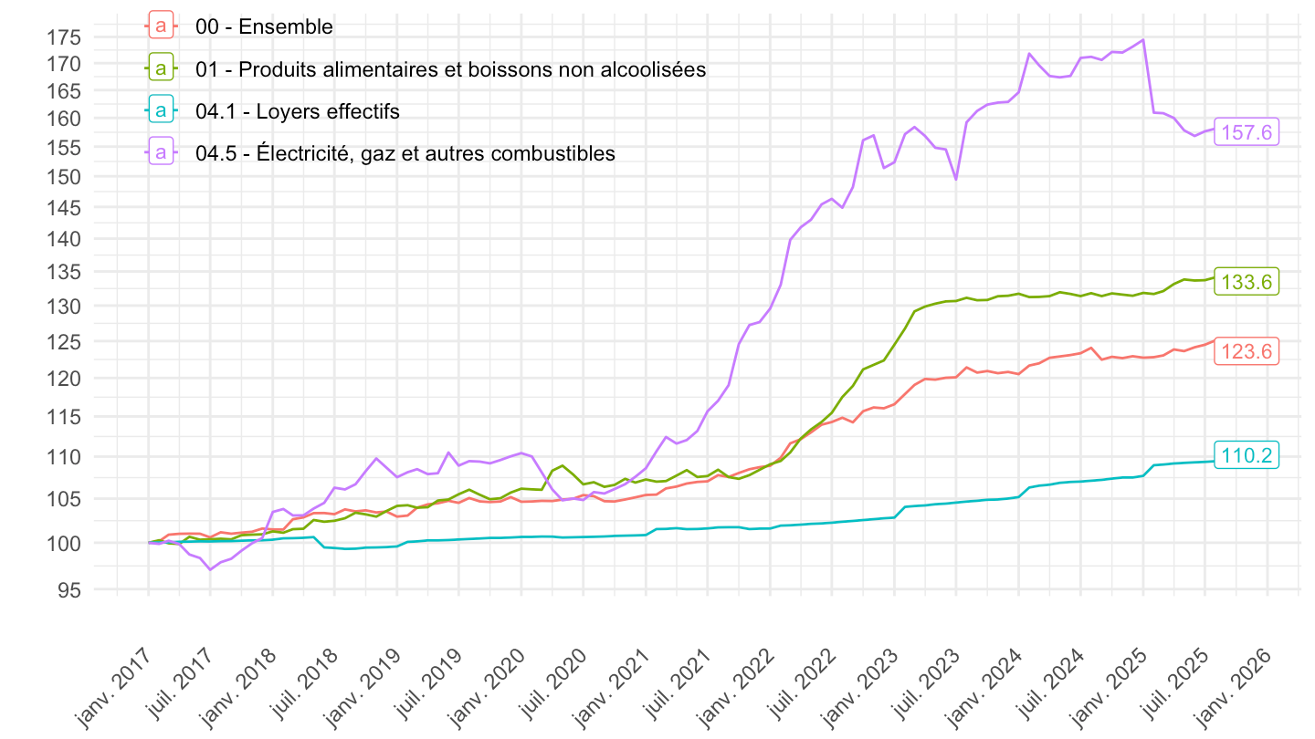
`IPCH-2015` |>
  filter(INDICATEUR == "IPCH",
         COICOP2016 %in% c("0452", "0451", "045"),
         FREQ == "M",
         NATURE == "INDICE") |>
  month_to_date() |>

  filter(date >= max(date) - years(30)) |>
  group_by(COICOP2016) |>
  arrange(date) |>
  mutate(OBS_VALUE = 100*OBS_VALUE/OBS_VALUE[1]) |>
  ggplot() + ylab("Indice des prix (J - 30 ans = 100)") + xlab("") + theme_minimal() +
  geom_line(aes(x = date, y = OBS_VALUE, color = Coicop2016)) +
  scale_x_date(breaks = "1 year",
               labels = date_format("%Y")) +
  theme(legend.position = c(0.3, 0.87),
        legend.title = element_blank(),
        axis.text.x = element_text(angle = 45, vjust = 0.5, hjust=1)) +
  scale_y_log10(breaks = seq(0, 10000, 20),
                     labels = dollar_format(accuracy = 1, prefix = "")) +
  geom_label(data = . %>% filter(date == max(date)),
                  aes(x = date, y = OBS_VALUE, label = round(OBS_VALUE, 1), color = Coicop2016),
                  fontface ="plain", size = 3)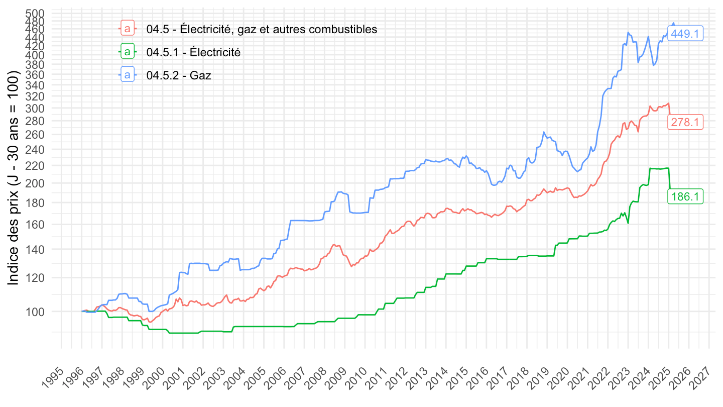
`IPCH-2015` |>
  filter(INDICATEUR == "IPCH",
         COICOP2016 %in% c("0452", "0451", "045"),
         FREQ == "M",
         NATURE == "INDICE") |>
  month_to_date() |>

  filter(date >= max(date) - years(20)) |>
  group_by(COICOP2016) |>
  arrange(date) |>
  mutate(OBS_VALUE = 100*OBS_VALUE/OBS_VALUE[1]) |>
  ggplot() + ylab("Indice des prix (J - 20 ans = 100)") + xlab("") + theme_minimal() +
  geom_line(aes(x = date, y = OBS_VALUE, color = Coicop2016)) +
  scale_x_date(breaks = "1 year",
               labels = date_format("%Y")) +
  theme(legend.position = c(0.3, 0.87),
        legend.title = element_blank(),
        axis.text.x = element_text(angle = 45, vjust = 0.5, hjust=1)) +
  scale_y_log10(breaks = seq(0, 10000, 20),
                     labels = dollar_format(accuracy = 1, prefix = "")) +
  geom_label(data = . %>% filter(date == max(date)),
                  aes(x = date, y = OBS_VALUE, label = round(OBS_VALUE, 1), color = Coicop2016),
                  fontface ="plain", size = 3)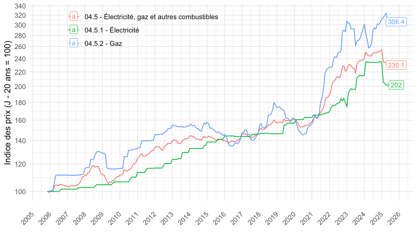
`IPCH-2015` |>
  filter(INDICATEUR == "IPCH",
         COICOP2016 %in% c("0452", "0451", "045"),
         FREQ == "M",
         NATURE == "INDICE") |>
  month_to_date() |>

  filter(date >= max(date) - years(10)) |>
  group_by(COICOP2016) |>
  arrange(date) |>
  mutate(OBS_VALUE = 100*OBS_VALUE/OBS_VALUE[1]) |>
  ggplot() + ylab("Indice des prix (J - 10 ans = 100)") + xlab("") + theme_minimal() +
  geom_line(aes(x = date, y = OBS_VALUE, color = Coicop2016)) +
  scale_x_date(breaks = "1 year",
               labels = date_format("%Y")) +
  theme(legend.position = c(0.3, 0.87),
        legend.title = element_blank(),
        axis.text.x = element_text(angle = 45, vjust = 0.5, hjust=1)) +
  scale_y_log10(breaks = seq(0, 10000, 20),
                     labels = dollar_format(accuracy = 1, prefix = "")) +
  geom_label(data = . %>% filter(date == max(date)),
                  aes(x = date, y = OBS_VALUE, label = round(OBS_VALUE, 1), color = Coicop2016),
                  fontface ="plain", size = 3)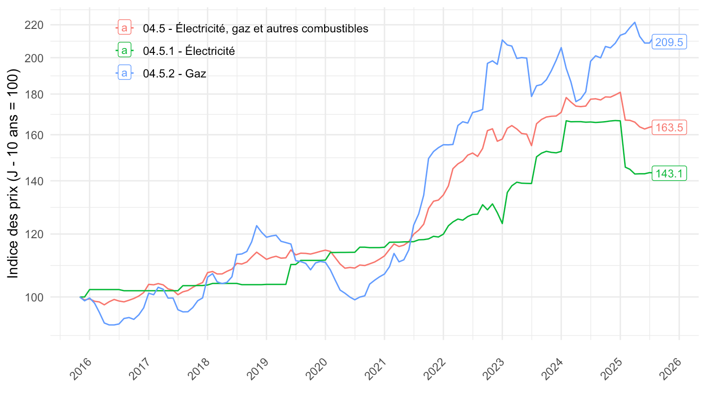
`IPCH-2015` |>
  filter(INDICATEUR == "IPCH",
         COICOP2016 %in% c("0452", "0451", "045"),
         FREQ == "M",
         NATURE == "INDICE") |>
  month_to_date() |>

  filter(date >= as.Date("2008-01-01")) |>
  group_by(COICOP2016) |>
  arrange(date) |>
  mutate(OBS_VALUE = 100*OBS_VALUE/OBS_VALUE[1]) |>
  ggplot() + ylab("Indice des prix (Janvier 2008 = 100)") + xlab("") + theme_minimal() +
  geom_line(aes(x = date, y = OBS_VALUE, color = Coicop2016)) +
  scale_x_date(breaks = "1 year",
               labels = date_format("%Y")) +
  theme(legend.position = c(0.3, 0.87),
        legend.title = element_blank(),
        axis.text.x = element_text(angle = 45, vjust = 0.5, hjust=1)) +
  scale_y_log10(breaks = seq(0, 10000, 20),
                     labels = dollar_format(accuracy = 1, prefix = "")) +
  geom_label(data = . %>% filter(date == max(date)),
                  aes(x = date, y = OBS_VALUE, label = round(OBS_VALUE, 1), color = Coicop2016),
                  fontface ="plain", size = 3)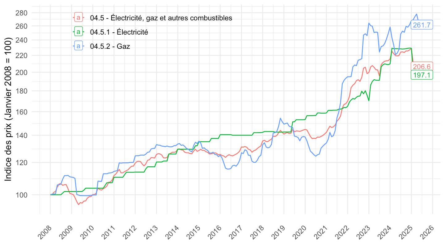
`IPCH-2015` |>
  filter(INDICATEUR == "IPCH",
         COICOP2016 %in% c("0452", "0451", "045"),
         FREQ == "M",
         NATURE == "INDICE") |>
  month_to_date() |>

  filter(date >= as.Date("2017-01-01")) |>
  group_by(COICOP2016) |>
  arrange(date) |>
  mutate(OBS_VALUE = 100*OBS_VALUE/OBS_VALUE[1]) |>
  ggplot() + ylab("Indice des prix (Janvier 2017 = 100)") + xlab("") + theme_minimal() +
  geom_line(aes(x = date, y = OBS_VALUE, color = Coicop2016)) +
  scale_x_date(breaks = "3 months",
               labels = date_format("%b %Y")) +
  theme(legend.position = c(0.25, 0.87),
        legend.title = element_blank(),
        axis.text.x = element_text(angle = 45, vjust = 0.5, hjust=1)) +
  scale_y_log10(breaks = seq(0, 10000, 5),
                     labels = dollar_format(accuracy = 1, prefix = "")) +
  geom_label(data = . %>% filter(date == max(date)),
                  aes(x = date, y = OBS_VALUE, label = round(OBS_VALUE, 1), color = Coicop2016),
                  fontface ="plain", size = 3)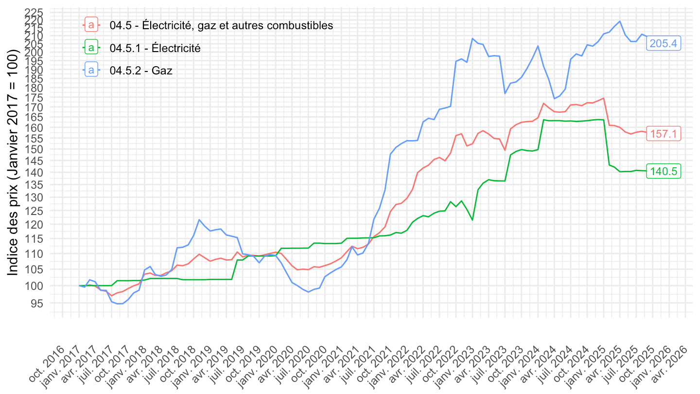
`IPCH-2015` |>
  filter(INDICATEUR == "IPCH",
         COICOP2016 %in% c("0452", "0451", "045"),
         FREQ == "M",
         NATURE == "INDICE") |>
  month_to_date() |>

  filter(date >= as.Date("2017-05-01")) |>
  group_by(COICOP2016) |>
  arrange(date) |>
  mutate(OBS_VALUE = 100*OBS_VALUE/OBS_VALUE[1]) |>
  ggplot() + ylab("Indice des prix (Mai 2017 = 100)") + xlab("") + theme_minimal() +
  geom_line(aes(x = date, y = OBS_VALUE, color = Coicop2016)) +
  scale_x_date(breaks = "3 months",
               labels = date_format("%b %Y")) +
  theme(legend.position = c(0.25, 0.87),
        legend.title = element_blank(),
        axis.text.x = element_text(angle = 45, vjust = 0.5, hjust=1)) +
  scale_y_log10(breaks = seq(0, 10000, 5),
                     labels = dollar_format(accuracy = 1, prefix = "")) +
  geom_label(data = . %>% filter(date == max(date)),
                  aes(x = date, y = OBS_VALUE, label = round(OBS_VALUE, 1), color = Coicop2016),
                  fontface ="plain", size = 3)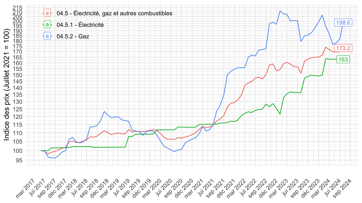
`IPCH-2015` |>
  filter(INDICATEUR == "IPCH",
         COICOP2016 %in% c("0452", "0451", "045"),
         FREQ == "M",
         NATURE == "INDICE") |>
  month_to_date() |>

  filter(date >= as.Date("2020-01-01")) |>
  group_by(COICOP2016) |>
  arrange(date) |>
  mutate(OBS_VALUE = 100*OBS_VALUE/OBS_VALUE[1]) |>
  ggplot() + ylab("Indice des prix (Janvier 2020 = 100)") + xlab("") + theme_minimal() +
  geom_line(aes(x = date, y = OBS_VALUE, color = Coicop2016)) +
  scale_x_date(breaks = "2 months",
               labels = date_format("%b %Y")) +
  theme(legend.position = c(0.25, 0.87),
        legend.title = element_blank(),
        axis.text.x = element_text(angle = 45, vjust = 0.5, hjust=1)) +
  scale_y_log10(breaks = seq(0, 200, 5),
                     labels = dollar_format(accuracy = 1, prefix = "")) +
  geom_label(data = . %>% filter(date == max(date)),
                  aes(x = date, y = OBS_VALUE, label = round(OBS_VALUE, 1), color = Coicop2016),
                  fontface ="plain", size = 3)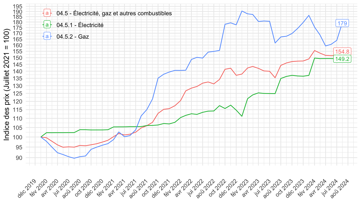
`IPCH-2015` |>
  filter(INDICATEUR == "IPCH",
         COICOP2016 %in% c("0452", "0451", "045"),
         FREQ == "M",
         NATURE == "INDICE") |>
  month_to_date() |>

  filter(date >= as.Date("2021-07-01")) |>
  group_by(COICOP2016) |>
  arrange(date) |>
  mutate(OBS_VALUE = 100*OBS_VALUE/OBS_VALUE[1]) |>
  ggplot() + ylab("Indice des prix (Juillet 2021 = 100)") + xlab("") + theme_minimal() +
  geom_line(aes(x = date, y = OBS_VALUE, color = Coicop2016)) +
  scale_x_date(breaks = "2 months",
               labels = date_format("%b %Y")) +
  theme(legend.position = c(0.25, 0.87),
        legend.title = element_blank(),
        axis.text.x = element_text(angle = 45, vjust = 0.5, hjust=1)) +
  scale_y_log10(breaks = seq(0, 200, 5),
                     labels = dollar_format(accuracy = 1, prefix = "")) +
  geom_label(data = . %>% filter(date == max(date)),
                  aes(x = date, y = OBS_VALUE, label = round(OBS_VALUE, 1), color = Coicop2016),
                  fontface ="plain", size = 3)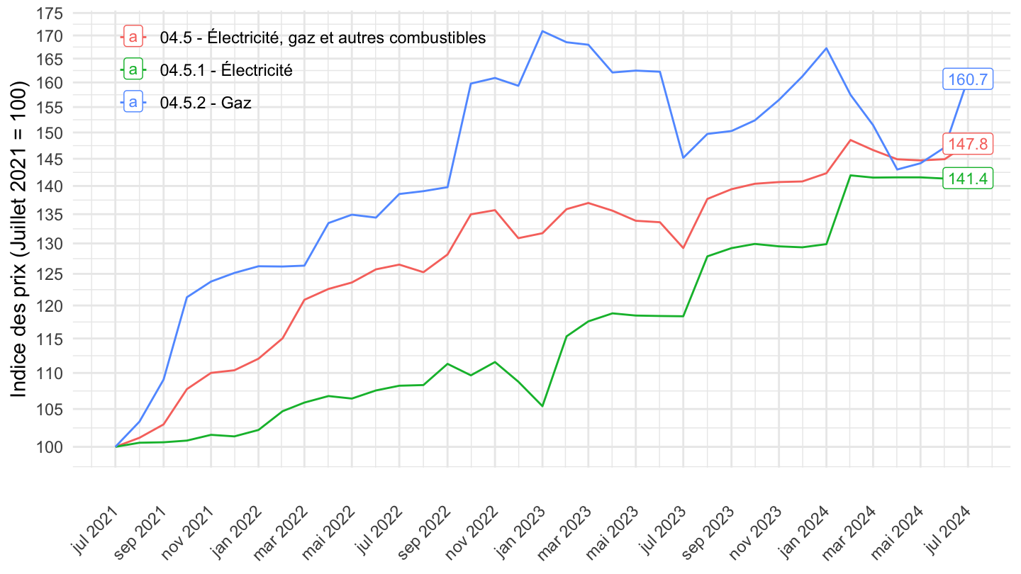
`IPCH-2015` |>
  filter(INDICATEUR == "IPCH",
         COICOP2016 %in% c("0452", "0451", "045"),
         FREQ == "M",
         NATURE == "INDICE") |>
  month_to_date() |>

  filter(date >= max(date) - years(3)) |>
  group_by(COICOP2016) |>
  arrange(date) |>
  mutate(OBS_VALUE = 100*OBS_VALUE/OBS_VALUE[1]) |>
  ggplot() + ylab("Indice des prix (Il y a 3 ans = 100)") + xlab("") + theme_minimal() +
  geom_line(aes(x = date, y = OBS_VALUE, color = Coicop2016)) +
  scale_x_date(breaks = "2 months",
               labels = date_format("%b %Y")) +
  theme(legend.position = c(0.25, 0.87),
        legend.title = element_blank(),
        axis.text.x = element_text(angle = 45, vjust = 0.5, hjust=1)) +
  scale_y_log10(breaks = seq(0, 200, 5),
                     labels = dollar_format(accuracy = 1, prefix = "")) +
  geom_label(data = . %>% filter(date == max(date)),
                  aes(x = date, y = OBS_VALUE, label = round(OBS_VALUE, 1), color = Coicop2016),
                  fontface ="plain", size = 3)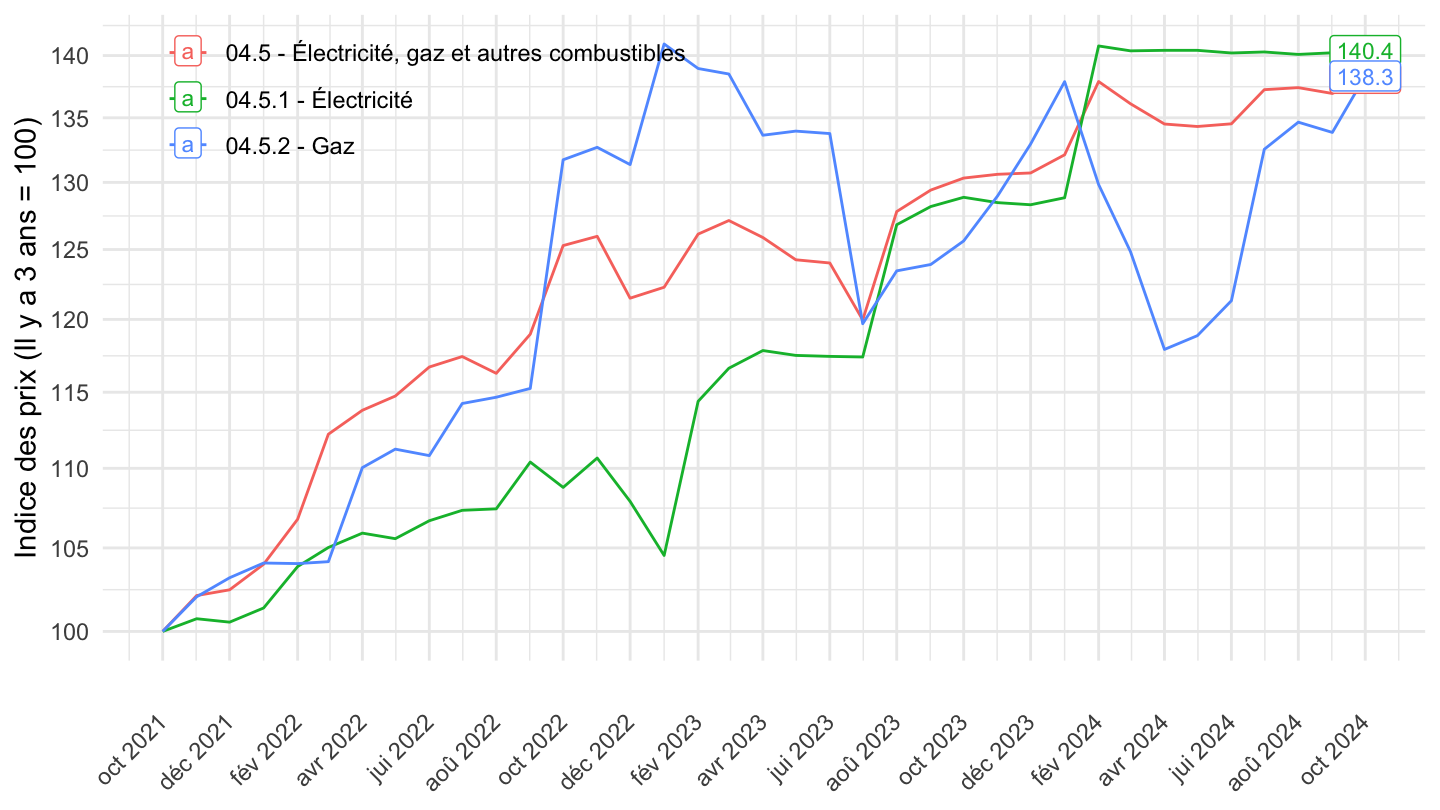
`IPCH-2015` |>
  filter(INDICATEUR == "IPCH",
         REF_AREA == "FE",
         NATURE == "POND",
         TIME_PERIOD %in% c("1990", "2000", "2010", "2020")) |>

  select(COICOP2016, Coicop2016, TIME_PERIOD, OBS_VALUE) |>
  spread(TIME_PERIOD, OBS_VALUE) |>
print_table_conditional()`IPCH-2015` |>
filter(INDICATEUR == "IPCH",
REF_AREA == "FE",
NATURE == "POND",
TIME_PERIOD %in% c("1990", "2000", "2010", "2020"),
nchar(COICOP2016) == 2) |>
select(COICOP2016, Coicop2016, TIME_PERIOD, OBS_VALUE) |>
spread(TIME_PERIOD, OBS_VALUE) |>
print_table_conditional()| COICOP2016 | Coicop2016 | 2000 | 2010 | 2020 |
|---|---|---|---|---|
| 00 | 00 - Ensemble | 10000 | 10000 | 10000 |
| 01 | 01 - Produits alimentaires et boissons non alcoolisées | 1695 | 1603 | 1592 |
| 02 | 02 - Boissons alcoolisées, tabac et stupéfiants | 412 | 357 | 442 |
| 03 | 03 - Articles d'habillement et chaussures | 588 | 531 | 439 |
| 04 | 04 - Logement, eau, gaz, électricité et autres combustibles | 1481 | 1467 | 1567 |
| 05 | 05 - Meubles, articles de ménage et entretien courant du foyer | 705 | 674 | 545 |
| 06 | 06 - Santé | 317 | 445 | 430 |
| 07 | 07 - Transports | 1802 | 1759 | 1735 |
| 08 | 08 - Communications | 273 | 330 | 276 |
| 09 | 09 - Loisirs et culture | 931 | 992 | 815 |
| 10 | 10 - Enseignement | 57 | 58 | 41 |
| 11 | 11 - Restaurants et hôtels | 870 | 740 | 899 |
| 12 | 12 - Biens et services divers | 869 | 1044 | 1219 |
`IPCH-2015` |>
  filter(INDICATEUR == "IPCH",
         COICOP2016 %in% c("06", "1253"),
         REF_AREA == "FE",
         NATURE == "POND") |>
  year_to_date() |>
  mutate(OBS_VALUE = OBS_VALUE/10000) |>
  ggplot() + ylab("Poids de la santé dans l'IPCH") + xlab("") + theme_minimal() +
  geom_line(aes(x = date, y = OBS_VALUE, color = Coicop2016)) +

  scale_x_date(breaks = seq(1920, 2100, 2) |> paste0("-01-01") |> as.Date(),
               labels = date_format("%Y")) +
  theme(legend.position = c(0.15, 0.9),
        legend.title = element_blank()) +
  scale_y_continuous(breaks = 0.01*seq(0, 20, 0.5),
                     labels = percent_format(accuracy = .1))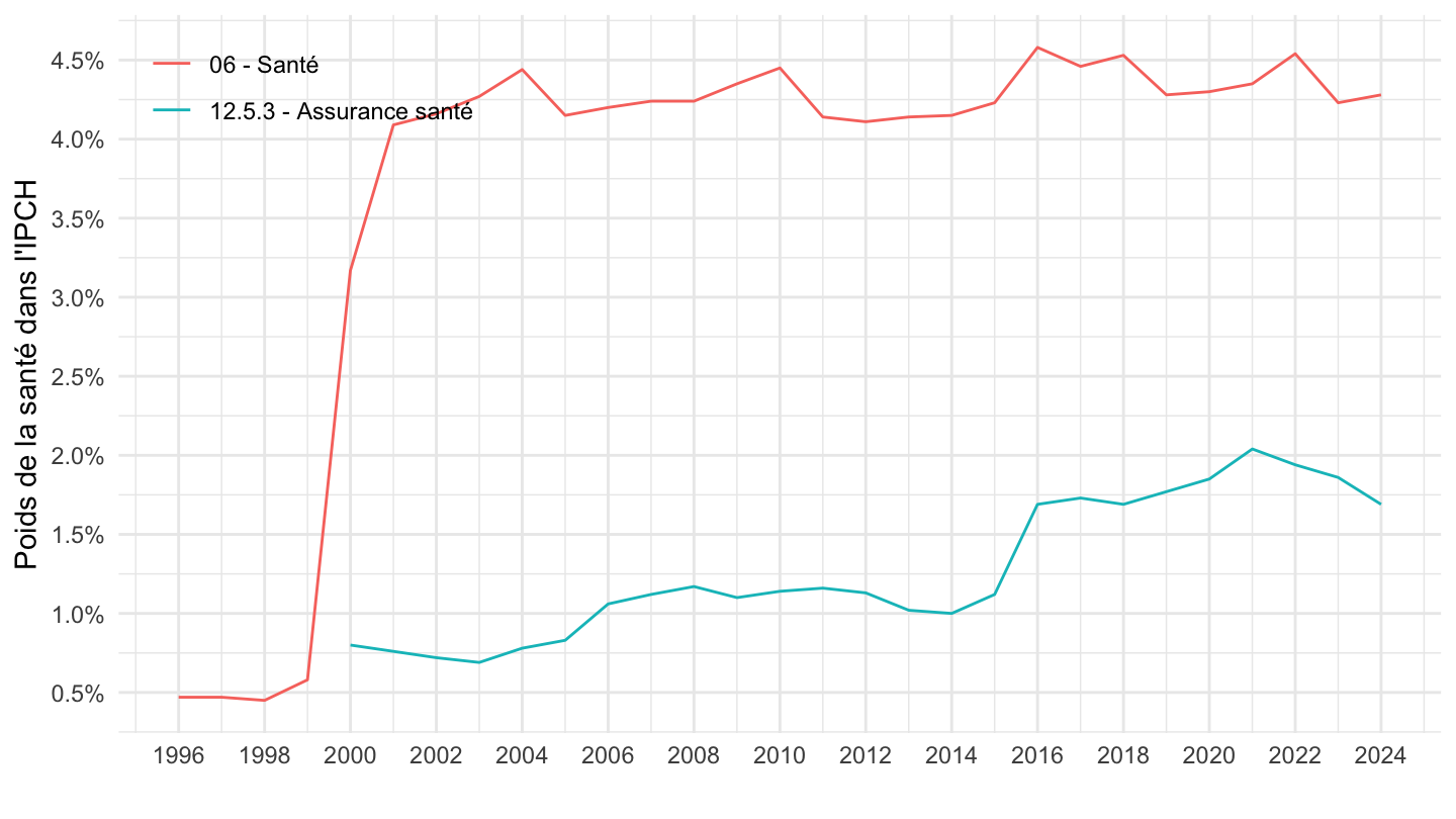
`IPCH-2015` |>
  filter(INDICATEUR == "IPCH",
         COICOP2016 %in% c("1112", "12401"),
         REF_AREA == "FE",
         NATURE == "POND") |>
  year_to_date() |>
  mutate(OBS_VALUE = OBS_VALUE/10000) |>
  ggplot() + ylab("Poids dans l'IPCH") + xlab("") + theme_minimal() +
  geom_line(aes(x = date, y = OBS_VALUE, color = Coicop2016)) +
  scale_x_date(breaks = seq(1920, 2100, 2) |> paste0("-01-01") |> as.Date(),
               labels = date_format("%Y")) +
  theme(legend.position = c(0.15, 0.9),
        legend.title = element_blank()) +
  scale_y_continuous(breaks = 0.01*seq(0, 20, 0.5),
                     labels = percent_format(accuracy = .1))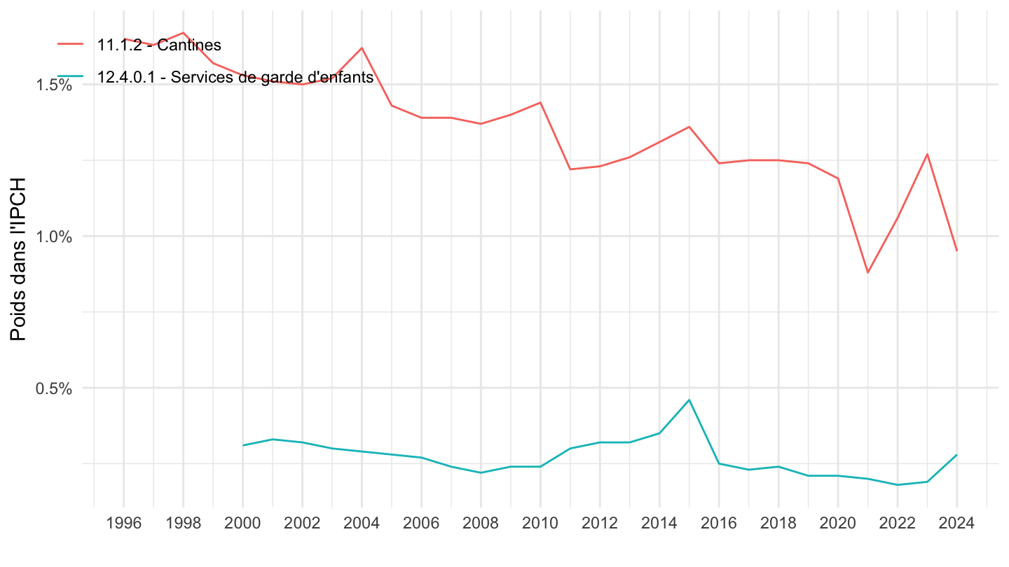
`IPCH-2015` |>
  bind_rows(`IPC-2015`) |>
  filter(COICOP2016 %in% c("1112", "12401"),
         NATURE == "POND",
         REF_AREA == "FE",
         is.na(MENAGES_IPC) | MENAGES_IPC == "ENSEMBLE") |>
  year_to_date() |>


  group_by(INDICATEUR) |>
  filter(date >= as.Date("1996-01-01")) |>
  arrange(date) |>
  ggplot() + ylab("Pondération - IPC vs. IPCH") + xlab("") + theme_minimal() +
  geom_line(aes(x = date, y = OBS_VALUE/10000, color =  Coicop2016, linetype = Indicateur)) +

  scale_x_date(breaks = seq(1920, 2100, 2) |> paste0("-01-01") |> as.Date(),
               labels = date_format("%Y")) +
  theme(legend.position = c(0.3, 0.55),
        legend.title = element_blank()) +
  scale_y_continuous(breaks = 0.01*seq(0, 300, .1),
                     labels = percent_format(accuracy = .1))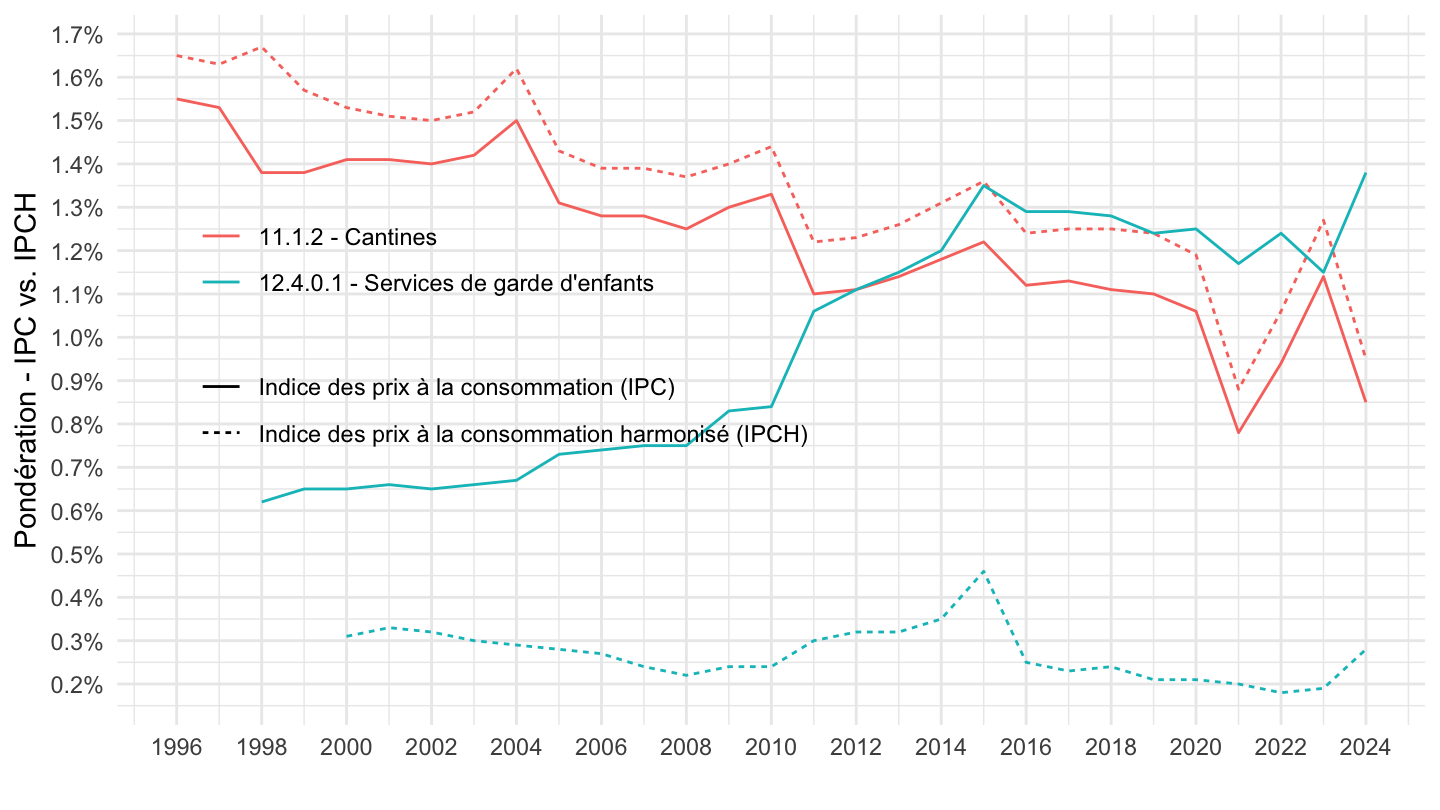
`IPCH-2015` |>
  filter(COICOP2016 %in% c("00", "02", "11", "04"),
         NATURE == "INDICE",
         FREQ == "M") |>
  month_to_date() |>

  group_by(COICOP2016) |>
  arrange(date) |>
  mutate(OBS_VALUE = 100*OBS_VALUE/OBS_VALUE[1]) |>
  ggplot() + ylab("Indice des prix") + xlab("") + theme_minimal() +
  geom_line(aes(x = date, y = OBS_VALUE, color = Coicop2016)) +

  scale_x_date(breaks = seq(1920, 2100, 2) |> paste0("-01-01") |> as.Date(),
               labels = date_format("%Y")) +
  theme(legend.position = c(0.3, 0.85),
        legend.title = element_blank()) +
  scale_y_log10(breaks = c(100, 120, 150, 200, 220, 250, 300, 400, 500),
                     labels = dollar_format(accuracy = 1, prefix = ""))
`IPCH-2015` |>
  filter(COICOP2016 %in% c("00", "10", "07", "12"),
         NATURE == "INDICE",
         FREQ == "M") |>
  month_to_date() |>

  group_by(COICOP2016) |>
  arrange(date) |>
  mutate(OBS_VALUE = 100*OBS_VALUE/OBS_VALUE[1]) |>
  ggplot() + ylab("Indice des prix") + xlab("") + theme_minimal() +
  geom_line(aes(x = date, y = OBS_VALUE, color = Coicop2016)) +

  scale_x_date(breaks = seq(1920, 2100, 2) |> paste0("-01-01") |> as.Date(),
               labels = date_format("%Y")) +
  theme(legend.position = c(0.3, 0.85),
        legend.title = element_blank()) +
  scale_y_log10(breaks = seq(100, 300, 10),
                     labels = dollar_format(accuracy = 1, prefix = ""))
`IPCH-2015` |>
  filter(COICOP2016 %in% c("00", "05", "01", "03"),
         NATURE == "INDICE",
         FREQ == "M") |>
  month_to_date() |>

  group_by(COICOP2016) |>
  arrange(date) |>
  mutate(OBS_VALUE = 100*OBS_VALUE/OBS_VALUE[1]) |>
  ggplot() + ylab("Indice des prix") + xlab("") + theme_minimal() +
  geom_line(aes(x = date, y = OBS_VALUE, color = Coicop2016)) +

  scale_x_date(breaks = seq(1920, 2100, 2) |> paste0("-01-01") |> as.Date(),
               labels = date_format("%Y")) +
  theme(legend.position = c(0.3, 0.85),
        legend.title = element_blank()) +
  scale_y_log10(breaks = seq(100, 300, 10),
                     labels = dollar_format(accuracy = 1, prefix = ""))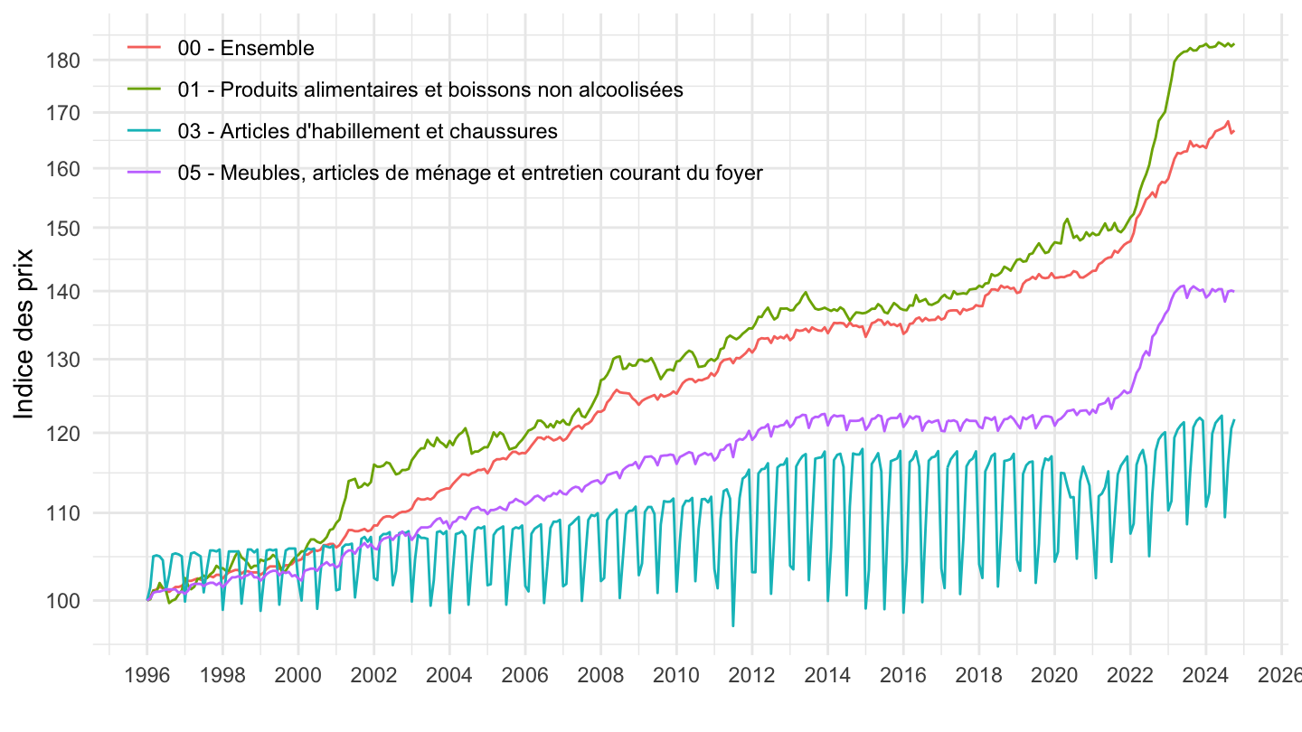
`IPCH-2015` |>
  filter(COICOP2016 %in% c("00", "06", "09", "08"),
         NATURE == "INDICE",
         FREQ == "M") |>
  month_to_date() |>

  group_by(COICOP2016) |>
  arrange(date) |>
  mutate(OBS_VALUE = 100*OBS_VALUE/OBS_VALUE[1]) |>
  ggplot() + ylab("Indice des prix") + xlab("") + theme_minimal() +
  geom_line(aes(x = date, y = OBS_VALUE, color = Coicop2016)) +

  scale_x_date(breaks = seq(1920, 2100, 2) |> paste0("-01-01") |> as.Date(),
               labels = date_format("%Y")) +
  theme(legend.position = c(0.2, 0.85),
        legend.title = element_blank()) +
  scale_y_log10(breaks = seq(10, 300, 10),
                     labels = dollar_format(accuracy = 1, prefix = ""))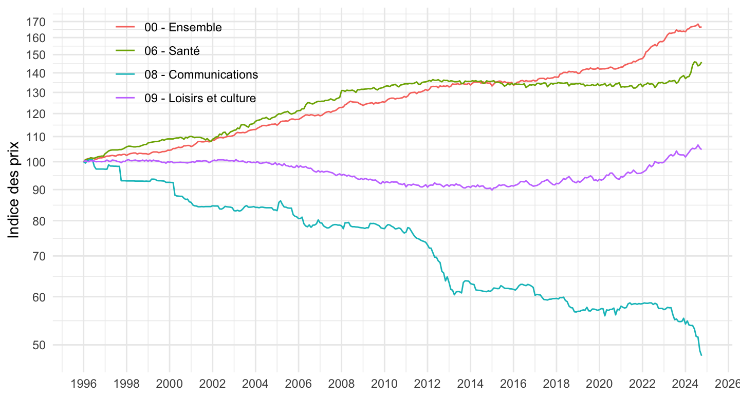
`IPCH-2015` |>
  bind_rows(`IPC-2015`) |>
  filter(COICOP2016 %in% c("06", "1253"),
         NATURE == "POND",
         REF_AREA == "FE",
         is.na(MENAGES_IPC) | MENAGES_IPC == "ENSEMBLE") |>
  year_to_date() |>


  group_by(INDICATEUR) |>
  filter(date >= as.Date("1996-01-01")) |>
  arrange(date) |>
  ggplot() + ylab("Pondération - Santé") + xlab("") + theme_minimal() +
  geom_line(aes(x = date, y = OBS_VALUE/10000, color =  Coicop2016, linetype = Indicateur)) +

  scale_x_date(breaks = seq(1920, 2100, 2) |> paste0("-01-01") |> as.Date(),
               labels = date_format("%Y")) +
  theme(legend.position = c(0.7, 0.6),
        legend.title = element_blank()) +
  scale_y_continuous(breaks = 0.01*seq(0, 300, 1),
                     labels = percent_format(accuracy = 1))
plot_sante_ponderation <- `IPCH-2015` |>
  bind_rows(`IPC-2015`) |>
  filter(COICOP2016 %in% c("06"),
         NATURE == "POND",
         REF_AREA == "FE",
         is.na(MENAGES_IPC) | MENAGES_IPC == "ENSEMBLE") |>
  year_to_date() |>

  group_by(INDICATEUR) |>
  filter(date >= as.Date("1996-01-01")) |>
  arrange(date) |>
  ggplot() + ylab("Pondération, 06 - Santé") + xlab("") + theme_minimal() +
  geom_line(aes(x = date, y = OBS_VALUE/10000, color = Indicateur)) +

  scale_x_date(breaks = seq(1920, 2100, 2) |> paste0("-01-01") |> as.Date(),
               labels = date_format("%Y")) +
  theme(legend.position = c(0.7, 0.55),
        legend.title = element_blank(),
        axis.text.x = element_text(angle = 45, vjust = 1, hjust = 1)) +
  scale_y_continuous(breaks = 0.01*seq(0, 300, 1),
                     labels = percent_format(accuracy = 1))

plot_sante_ponderation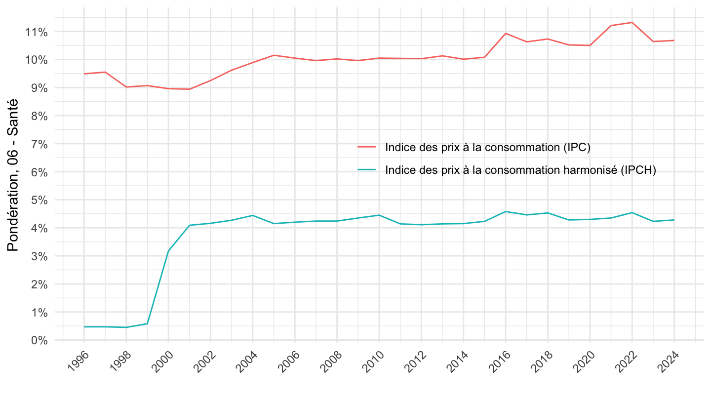
`IPCH-2015` |>
  bind_rows(`IPC-2015`) |>
  filter(COICOP2016 %in% c("061"),
         NATURE == "POND",
         REF_AREA == "FE",
         is.na(MENAGES_IPC) | MENAGES_IPC == "ENSEMBLE") |>
  year_to_date() |>

  group_by(INDICATEUR) |>
  filter(date >= as.Date("1996-01-01")) |>
  arrange(date) |>
  ggplot() + ylab("Pondération, 061 - Produits médicaux") + xlab("") + theme_minimal() +
  geom_line(aes(x = date, y = OBS_VALUE/10000, color = Indicateur)) +

  scale_x_date(breaks = seq(1920, 2100, 2) |> paste0("-01-01") |> as.Date(),
               labels = date_format("%Y")) +
  theme(legend.position = c(0.7, 0.55),
        legend.title = element_blank()) +
  scale_y_continuous(breaks = 0.01*seq(0, 300, 1),
                     labels = percent_format(accuracy = 1))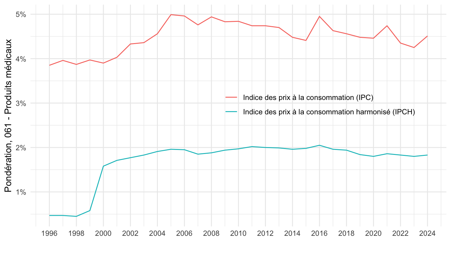
`IPCH-2015` |>
  bind_rows(`IPC-2015`) |>
  filter(COICOP2016 %in% c("062"),
         NATURE == "POND",
         REF_AREA == "FE",
         is.na(MENAGES_IPC) | MENAGES_IPC == "ENSEMBLE") |>
  year_to_date() |>

  group_by(INDICATEUR) |>
  filter(date >= as.Date("1996-01-01")) |>
  arrange(date) |>
  ggplot() + ylab("Pondération, 062 - Services médicaux") + xlab("") + theme_minimal() +
  geom_line(aes(x = date, y = OBS_VALUE/10000, color = Indicateur)) +

  scale_x_date(breaks = seq(1920, 2100, 2) |> paste0("-01-01") |> as.Date(),
               labels = date_format("%Y")) +
  theme(legend.position = c(0.7, 0.55),
        legend.title = element_blank()) +
  scale_y_continuous(breaks = 0.01*seq(0, 300, 1),
                     labels = percent_format(accuracy = 1))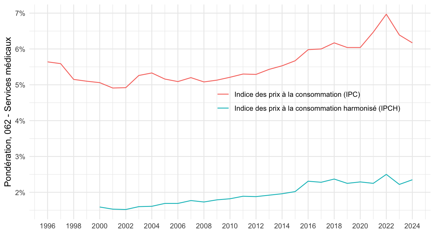
`IPCH-2015` |>
  bind_rows(`IPC-2015`) |>
  filter(COICOP2016 %in% c("0611"),
         NATURE == "POND",
         REF_AREA == "FE",
         is.na(MENAGES_IPC) | MENAGES_IPC == "ENSEMBLE") |>
  year_to_date() |>

  group_by(INDICATEUR) |>
  filter(date >= as.Date("1996-01-01")) |>
  arrange(date) |>
  ggplot() + ylab("Pondération, 0611 - Produits pharmaceutiques") + xlab("") + theme_minimal() +
  geom_line(aes(x = date, y = OBS_VALUE/10000, color = Indicateur)) +

  scale_x_date(breaks = seq(1920, 2100, 2) |> paste0("-01-01") |> as.Date(),
               labels = date_format("%Y")) +
  theme(legend.position = c(0.7, 0.55),
        legend.title = element_blank()) +
  scale_y_continuous(breaks = 0.01*seq(0, 300, 1),
                     labels = percent_format(accuracy = 1))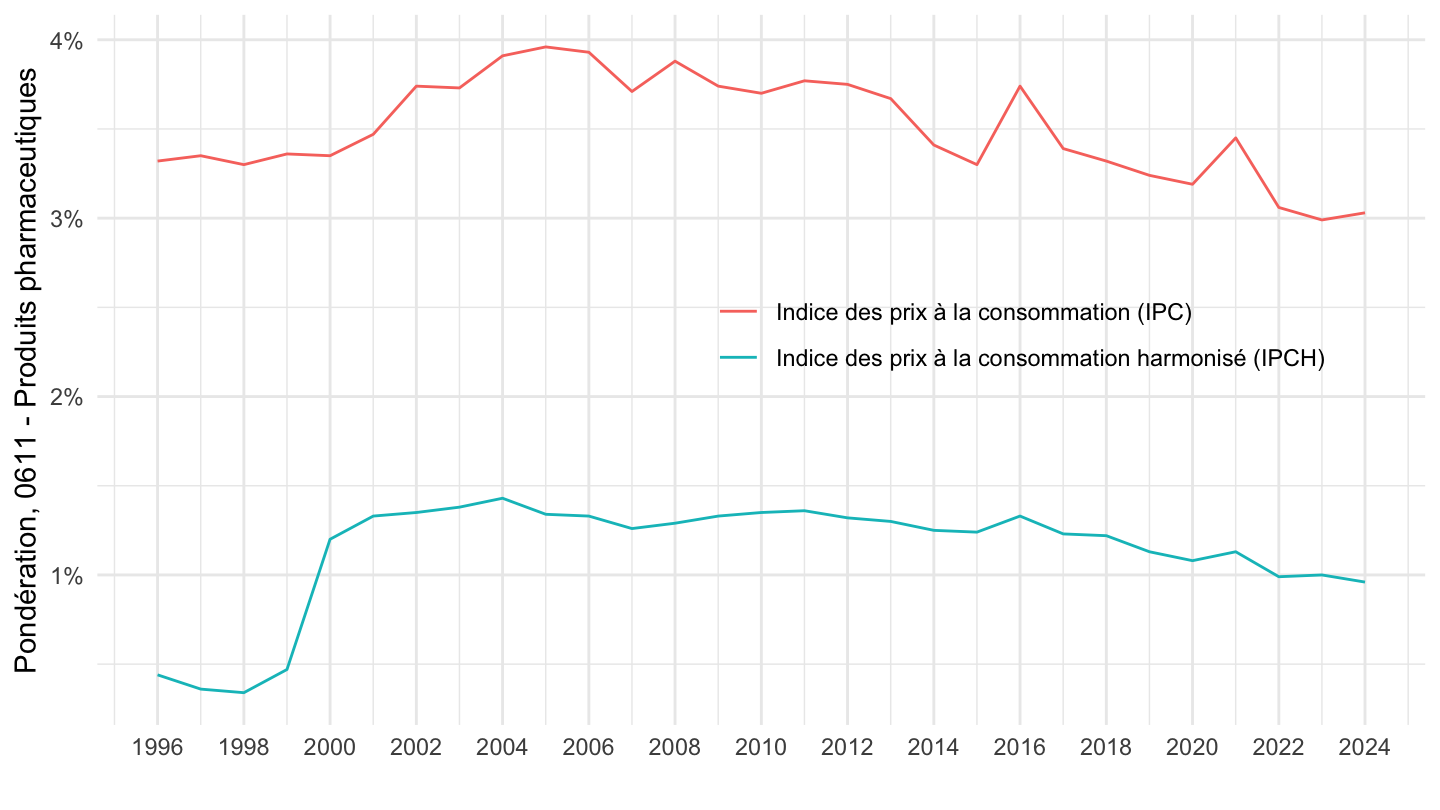
`IPCH-2015` |>
  bind_rows(`IPC-2015`) |>
  filter(COICOP2016 %in% c("0612"),
         NATURE == "POND",
         REF_AREA == "FE",
         is.na(MENAGES_IPC) | MENAGES_IPC == "ENSEMBLE") |>
  year_to_date() |>

  group_by(INDICATEUR) |>
  filter(date >= as.Date("1996-01-01")) |>
  arrange(date) |>
  ggplot() + ylab("Pondération des produits médicaux divers l'IPC, IPCH") + xlab("") + theme_minimal() +
  geom_line(aes(x = date, y = OBS_VALUE/10000, color = Indicateur)) +

  scale_x_date(breaks = seq(1920, 2100, 2) |> paste0("-01-01") |> as.Date(),
               labels = date_format("%Y")) +
  theme(legend.position = c(0.3, 0.9),
        legend.title = element_blank()) +
  scale_y_continuous(breaks = 0.01*seq(0, 300, .1),
                     labels = percent_format(accuracy = .1))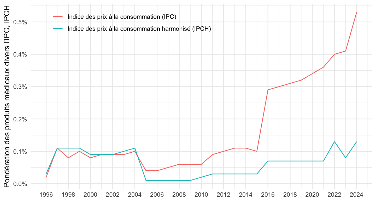
`IPCH-2015` |>
  bind_rows(`IPC-2015`) |>
  filter(COICOP2016 %in% c("0613"),
         NATURE == "POND",
         REF_AREA == "FE",
         is.na(MENAGES_IPC) | MENAGES_IPC == "ENSEMBLE") |>
  year_to_date() |>

  group_by(INDICATEUR) |>
  filter(date >= as.Date("1996-01-01")) |>
  arrange(date) |>
  ggplot() + ylab("Pondération des Appareils et matériel thérapeutiques l'IPC, IPCH") + xlab("") + theme_minimal() +
  geom_line(aes(x = date, y = OBS_VALUE/10000, color = Indicateur)) +

  scale_x_date(breaks = seq(1920, 2100, 2) |> paste0("-01-01") |> as.Date(),
               labels = date_format("%Y")) +
  theme(legend.position = c(0.7, 0.55),
        legend.title = element_blank()) +
  scale_y_continuous(breaks = 0.01*seq(0, 300, .1),
                     labels = percent_format(accuracy = .1))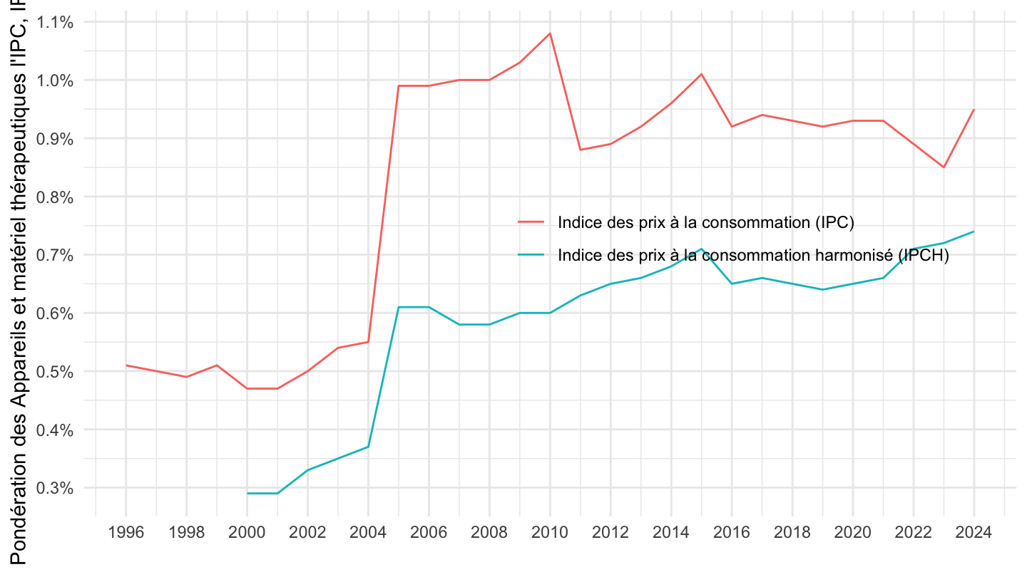
`IPCH-2015` |>
  bind_rows(`IPC-2015`) |>
  filter(COICOP2016 %in% c("0621"),
         NATURE == "POND",
         REF_AREA == "FE",
         is.na(MENAGES_IPC) | MENAGES_IPC == "ENSEMBLE") |>
  year_to_date() |>

  group_by(INDICATEUR) |>
  filter(date >= as.Date("1996-01-01")) |>
  arrange(date) |>
  ggplot() + ylab("Pondération des Appareils et matériel thérapeutiques l'IPC, IPCH") + xlab("") + theme_minimal() +
  geom_line(aes(x = date, y = OBS_VALUE/10000, color = Indicateur)) +

  scale_x_date(breaks = seq(1920, 2100, 2) |> paste0("-01-01") |> as.Date(),
               labels = date_format("%Y")) +
  theme(legend.position = c(0.7, 0.55),
        legend.title = element_blank()) +
  scale_y_continuous(breaks = 0.01*seq(0, 300, .1),
                     labels = percent_format(accuracy = .1))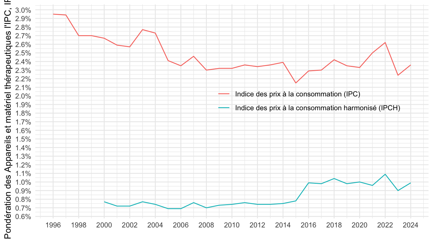
`IPCH-2015` |>
  bind_rows(`IPC-2015`) |>
  filter(COICOP2016 %in% c("0622"),
         NATURE == "POND",
         REF_AREA == "FE",
         is.na(MENAGES_IPC) | MENAGES_IPC == "ENSEMBLE") |>
  year_to_date() |>

  group_by(INDICATEUR) |>
  filter(date >= as.Date("1996-01-01")) |>
  arrange(date) |>
  ggplot() + ylab("Pondération des Appareils et matériel thérapeutiques l'IPC, IPCH") + xlab("") + theme_minimal() +
  geom_line(aes(x = date, y = OBS_VALUE/10000, color = Indicateur)) +

  scale_x_date(breaks = seq(1920, 2100, 2) |> paste0("-01-01") |> as.Date(),
               labels = date_format("%Y")) +
  theme(legend.position = c(0.7, 0.55),
        legend.title = element_blank()) +
  scale_y_continuous(breaks = 0.01*seq(0, 300, .1),
                     labels = percent_format(accuracy = .1))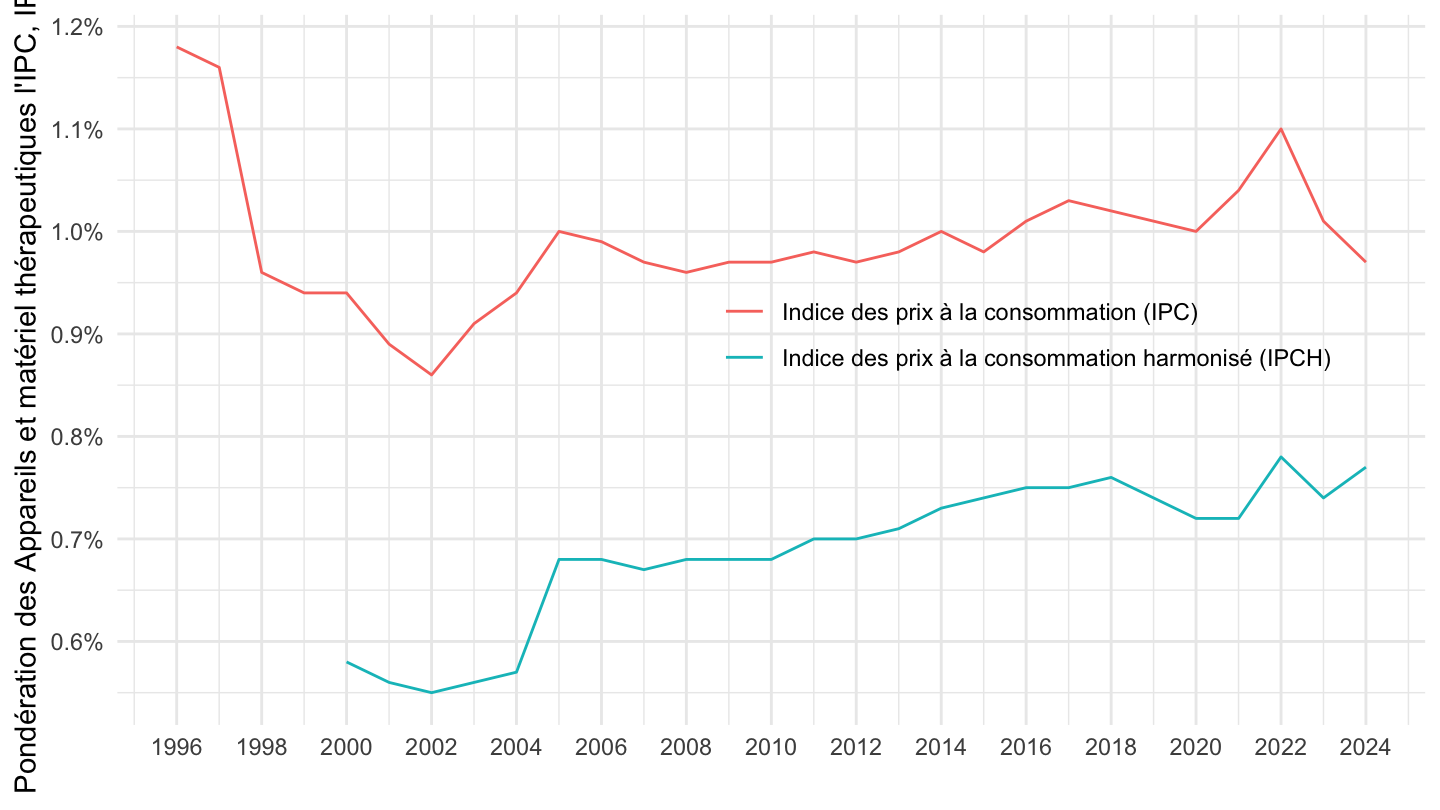
`IPCH-2015` |>
  bind_rows(`IPC-2015`) |>
  filter(COICOP2016 %in% c("0623"),
         NATURE == "POND",
         REF_AREA == "FE",
         is.na(MENAGES_IPC) | MENAGES_IPC == "ENSEMBLE") |>
  year_to_date() |>

  group_by(INDICATEUR) |>
  filter(date >= as.Date("1996-01-01")) |>
  arrange(date) |>
  ggplot() + ylab("Pondération des Appareils et matériel thérapeutiques l'IPC, IPCH") + xlab("") + theme_minimal() +
  geom_line(aes(x = date, y = OBS_VALUE/10000, color = Indicateur)) +

  scale_x_date(breaks = seq(1920, 2100, 2) |> paste0("-01-01") |> as.Date(),
               labels = date_format("%Y")) +
  theme(legend.position = c(0.7, 0.55),
        legend.title = element_blank()) +
  scale_y_continuous(breaks = 0.01*seq(0, 300, .1),
                     labels = percent_format(accuracy = .1))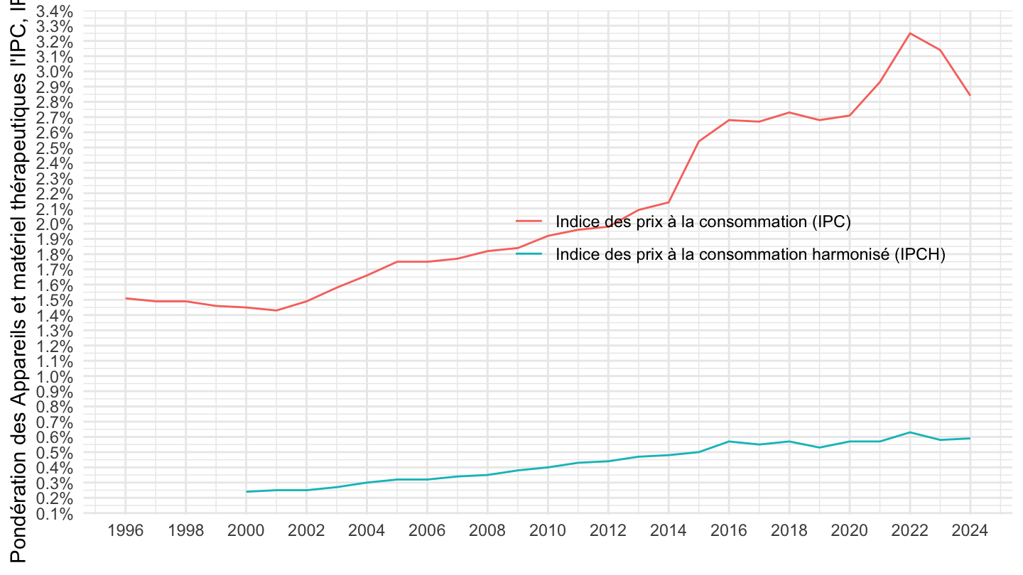
`IPCH-2015` |>
  bind_rows(`IPC-2015`) |>
  filter(COICOP2016 %in% c("10", "101", "102", "104"),
         NATURE == "POND",
         REF_AREA == "FE",
         is.na(MENAGES_IPC) | MENAGES_IPC == "ENSEMBLE") |>
  year_to_date() |>


  group_by(INDICATEUR) |>
  filter(date >= as.Date("1996-01-01")) |>
  arrange(date) |>
  ggplot() + ylab("") + xlab("") + theme_minimal() +
  geom_line(aes(x = date, y = OBS_VALUE/10000, color =  Coicop2016, linetype = Indicateur)) +

  scale_x_date(breaks = seq(1920, 2100, 2) |> paste0("-01-01") |> as.Date(),
               labels = date_format("%Y")) +
  theme(legend.position = c(0.3, 0.8),
        legend.title = element_blank()) +
  scale_y_continuous(breaks = 0.01*seq(0, 300, .1),
                     labels = percent_format(accuracy = .1))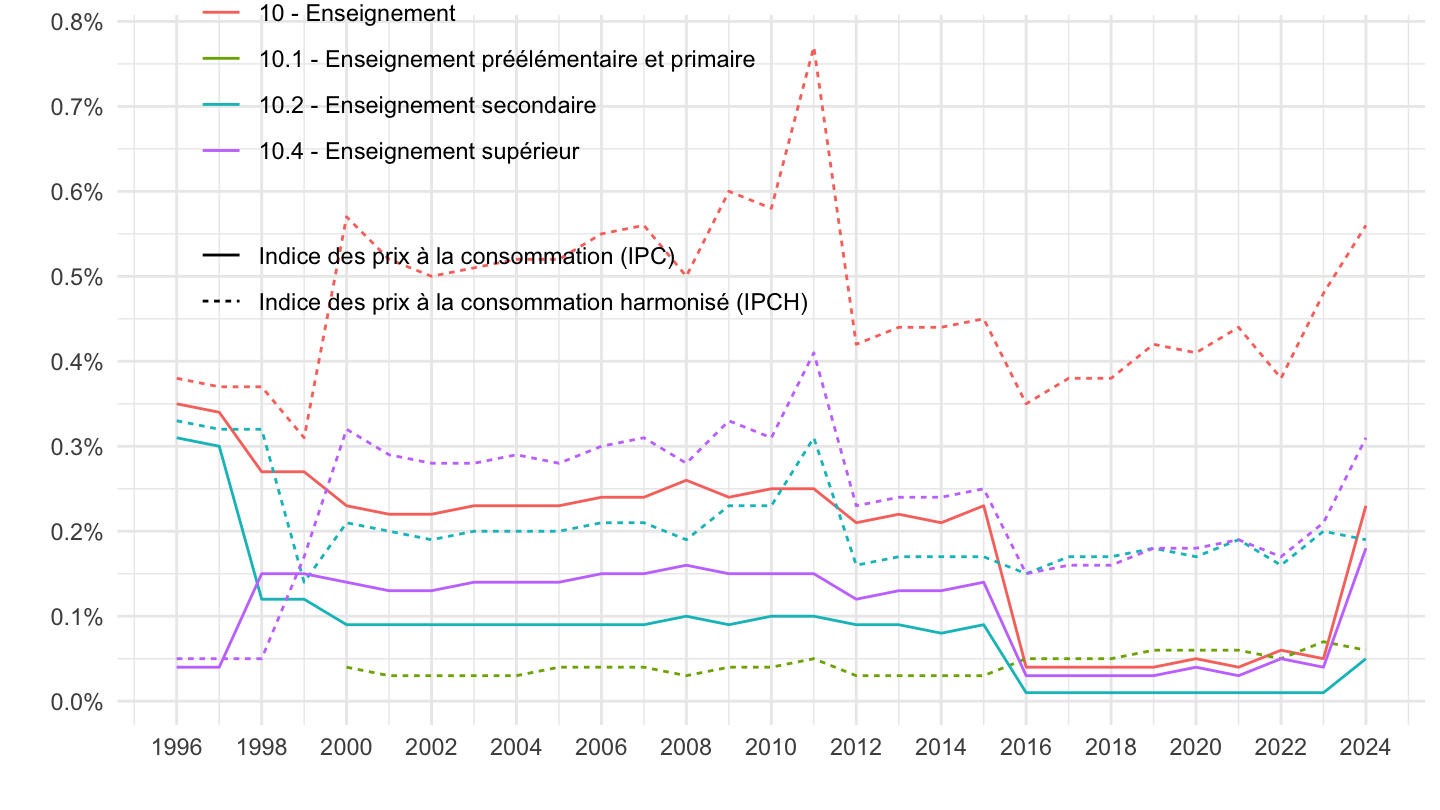
`IPCH-2015` |>
  bind_rows(`IPC-2015`) |>
  filter(COICOP2016 %in% c("10"),
         NATURE == "POND",
         REF_AREA == "FE",
         is.na(MENAGES_IPC) | MENAGES_IPC == "ENSEMBLE") |>
  year_to_date() |>

  group_by(INDICATEUR) |>
  filter(date >= as.Date("1996-01-01")) |>
  arrange(date) |>
  ggplot() + ylab("Pondération de l'Enseignement dans l'IPC, IPCH") + xlab("") + theme_minimal() +
  geom_line(aes(x = date, y = OBS_VALUE/10000, color = Indicateur)) +

  scale_x_date(breaks = seq(1920, 2100, 2) |> paste0("-01-01") |> as.Date(),
               labels = date_format("%Y")) +
  theme(legend.position = c(0.28, 0.95),
        legend.title = element_blank()) +
  scale_y_continuous(breaks = 0.01*seq(0, 300, .1),
                     labels = percent_format(accuracy = .1))
`IPCH-2015` |>
  bind_rows(`IPC-2015`) |>
  filter(COICOP2016 %in% c("101"),
         NATURE == "POND",
         REF_AREA == "FE",
         is.na(MENAGES_IPC) | MENAGES_IPC == "ENSEMBLE") |>
  year_to_date() |>

  group_by(INDICATEUR) |>
  filter(date >= as.Date("1996-01-01")) |>
  arrange(date) |>
  ggplot() + ylab("Pondération de l'Enseignement Primaire dans l'IPC, IPCH") + xlab("") + theme_minimal() +
  geom_line(aes(x = date, y = OBS_VALUE/10000, color = Indicateur)) +

  scale_x_date(breaks = seq(1920, 2100, 2) |> paste0("-01-01") |> as.Date(),
               labels = date_format("%Y")) +
  theme(legend.position = c(0.28, 0.95),
        legend.title = element_blank()) +
  scale_y_continuous(breaks = 0.01*seq(0, 300, .01),
                     labels = percent_format(accuracy = .01))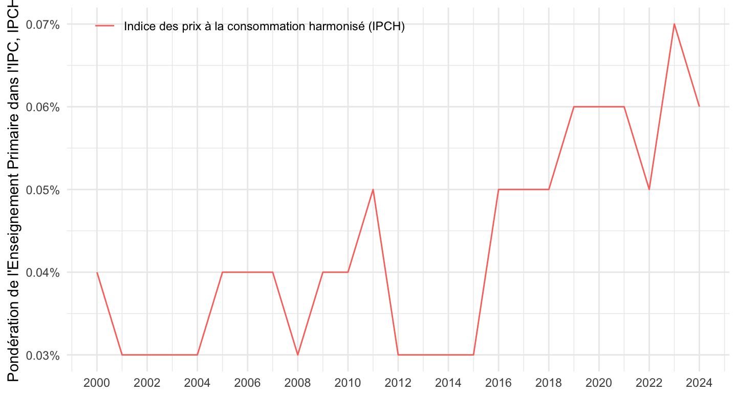
`IPCH-2015` |>
  bind_rows(`IPC-2015`) |>
  filter(COICOP2016 %in% c("102"),
         NATURE == "POND",
         REF_AREA == "FE",
         is.na(MENAGES_IPC) | MENAGES_IPC == "ENSEMBLE") |>
  year_to_date() |>

  group_by(INDICATEUR) |>
  filter(date >= as.Date("1996-01-01")) |>
  arrange(date) |>
  ggplot() + ylab("Pondération de l'Enseignement Secondaire dans l'IPC, IPCH") + xlab("") + theme_minimal() +
  geom_line(aes(x = date, y = OBS_VALUE/10000, color = Indicateur)) +

  scale_x_date(breaks = seq(1920, 2100, 2) |> paste0("-01-01") |> as.Date(),
               labels = date_format("%Y")) +
  theme(legend.position = c(0.28, 0.95),
        legend.title = element_blank()) +
  scale_y_continuous(breaks = 0.01*seq(0, 300, .02),
                     labels = percent_format(accuracy = .01))
`IPCH-2015` |>
  bind_rows(`IPC-2015`) |>
  filter(COICOP2016 %in% c("104"),
         NATURE == "POND",
         REF_AREA == "FE",
         is.na(MENAGES_IPC) | MENAGES_IPC == "ENSEMBLE") |>
  year_to_date() |>

  group_by(INDICATEUR) |>
  filter(date >= as.Date("1996-01-01")) |>
  arrange(date) |>
  ggplot() + ylab("Pondération de l'Enseignement Supérieur dans l'IPC, IPCH") + xlab("") + theme_minimal() +
  geom_line(aes(x = date, y = OBS_VALUE/10000, color = Indicateur)) +

  scale_x_date(breaks = seq(1920, 2100, 2) |> paste0("-01-01") |> as.Date(),
               labels = date_format("%Y")) +
  theme(legend.position = c(0.28, 0.95),
        legend.title = element_blank()) +
  scale_y_continuous(breaks = 0.01*seq(0, 300, .02),
                     labels = percent_format(accuracy = .01))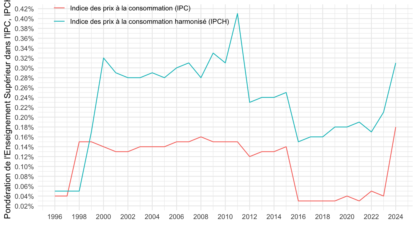
`IPCH-2015` |>
  bind_rows(`IPC-2015`) |>
  filter(COICOP2016 %in% c("09"),
         NATURE == "POND",
         REF_AREA == "FE",
         is.na(MENAGES_IPC) | MENAGES_IPC == "ENSEMBLE") |>
  year_to_date() |>

  group_by(INDICATEUR) |>
  filter(date >= as.Date("1996-01-01")) |>
  arrange(date) |>
  ggplot() + ylab("Pondération de la Santé dans l'IPC, IPCH") + xlab("") + theme_minimal() +
  geom_line(aes(x = date, y = OBS_VALUE/10000, color = Indicateur)) +

  scale_x_date(breaks = seq(1920, 2100, 2) |> paste0("-01-01") |> as.Date(),
               labels = date_format("%Y")) +
  theme(legend.position = c(0.7, 0.85),
        legend.title = element_blank()) +
  scale_y_continuous(breaks = 0.01*seq(0, 300, .5),
                     labels = percent_format(accuracy = .1))
`IPCH-2015` |>
  bind_rows(`IPC-2015`) |>
  filter(COICOP2016 %in% c("05"),
         NATURE == "POND",
         REF_AREA == "FE",
         is.na(MENAGES_IPC) | MENAGES_IPC == "ENSEMBLE") |>
  year_to_date() |>

  group_by(INDICATEUR) |>
  filter(date >= as.Date("1996-01-01")) |>
  arrange(date) |>
  ggplot() + ylab("Pondération de 05 dans l'IPC, IPCH") + xlab("") + theme_minimal() +
  geom_line(aes(x = date, y = OBS_VALUE/10000, color = Indicateur)) +

  scale_x_date(breaks = seq(1920, 2100, 2) |> paste0("-01-01") |> as.Date(),
               labels = date_format("%Y")) +
  theme(legend.position = c(0.7, 0.85),
        legend.title = element_blank()) +
  scale_y_continuous(breaks = 0.01*seq(0, 300, .5),
                     labels = percent_format(accuracy = .1))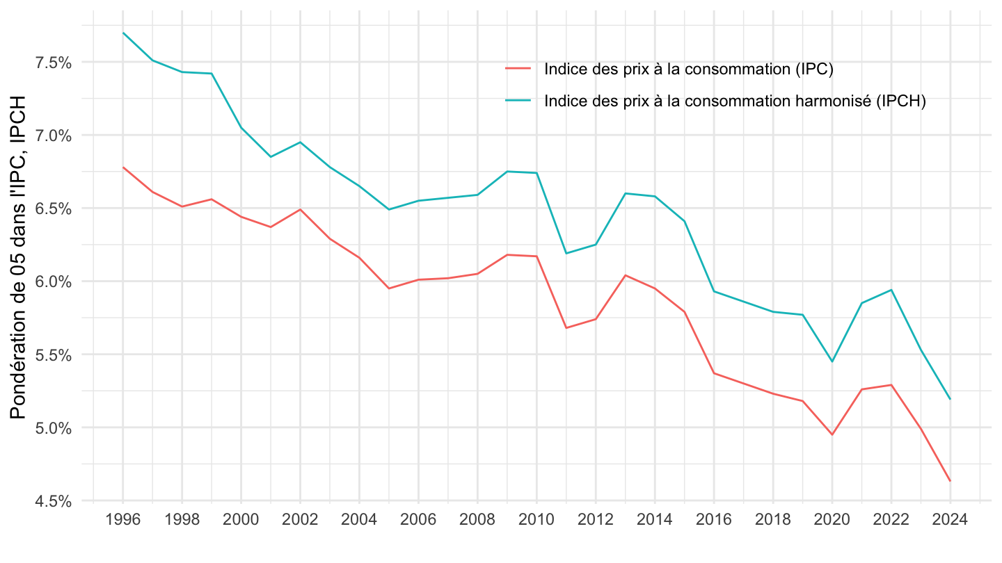
`IPCH-2015` |>
  bind_rows(`IPC-2015`) |>
  filter(COICOP2016 %in% c("0562"),
         NATURE == "POND",
         REF_AREA == "FE",
         is.na(MENAGES_IPC) | MENAGES_IPC == "ENSEMBLE") |>
  year_to_date() |>

  group_by(INDICATEUR) |>
  filter(date >= as.Date("1996-01-01")) |>
  arrange(date) |>
  ggplot() + ylab("Pondération de 05 dans l'IPC, IPCH") + xlab("") + theme_minimal() +
  geom_line(aes(x = date, y = OBS_VALUE/10000, color = Indicateur)) +

  scale_x_date(breaks = seq(1920, 2100, 2) |> paste0("-01-01") |> as.Date(),
               labels = date_format("%Y")) +
  theme(legend.position = c(0.7, 0.85),
        legend.title = element_blank()) +
  scale_y_continuous(breaks = 0.01*seq(0, 300, .1),
                     labels = percent_format(accuracy = .1))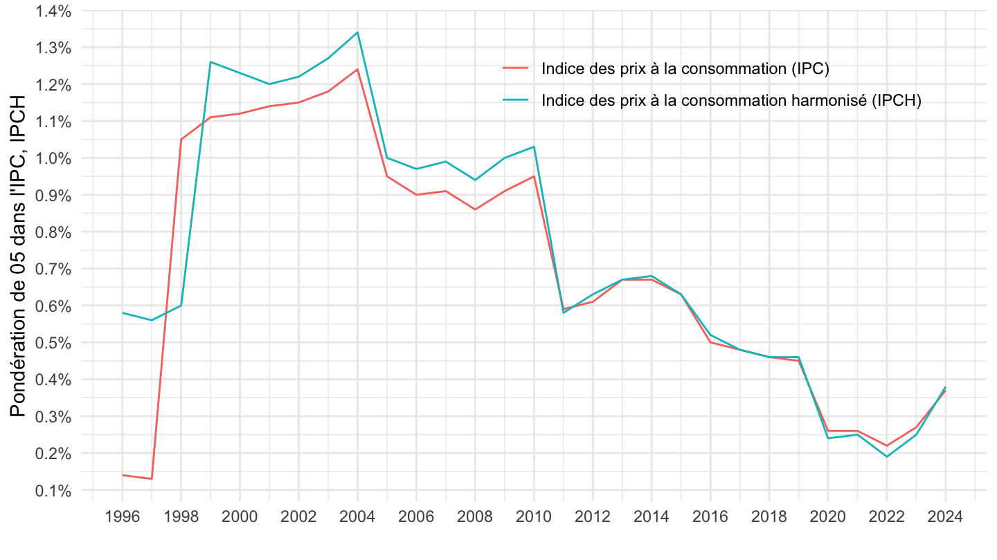
`IPCH-2015` |>
  bind_rows(`IPC-2015`) |>
  filter(COICOP2016 %in% c("01"),
         NATURE == "POND",
         REF_AREA == "FE",
         is.na(MENAGES_IPC) | MENAGES_IPC == "ENSEMBLE") |>
  year_to_date() |>

  group_by(INDICATEUR) |>
  arrange(date) |>
  ggplot() + ylab("Pondération de l'Alimentation dans l'IPC, IPCH") + xlab("") + theme_minimal() +
  geom_line(aes(x = date, y = OBS_VALUE/10000, color = Indicateur)) +

  scale_x_date(breaks = seq(1920, 2100, 2) |> paste0("-01-01") |> as.Date(),
               labels = date_format("%Y")) +
  theme(legend.position = c(0.7, 0.85),
        legend.title = element_blank()) +
  scale_y_continuous(breaks = 0.01*seq(0, 300, .5),
                     labels = percent_format(accuracy = .1)) +
  geom_text_repel(aes(x = date, y = OBS_VALUE/10000, label = percent(OBS_VALUE/10000, acc = 0.1)),
                  fontface ="plain", color = "black", size = 3)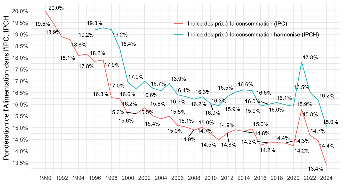
`IPCH-2015` |>
  bind_rows(`IPC-2015`) |>
  filter(COICOP2016 %in% c("01"),
         NATURE == "POND",
         REF_AREA == "FE",
         is.na(MENAGES_IPC) | MENAGES_IPC == "ENSEMBLE") |>
  year_to_date() |>

  group_by(INDICATEUR) |>
  filter(date >= as.Date("1996-01-01")) |>
  arrange(date) |>
  ggplot() + ylab("Pondération de l'Alimentation dans l'IPC, IPCH") + xlab("") + theme_minimal() +
  geom_line(aes(x = date, y = OBS_VALUE/10000, color = Indicateur)) +

  scale_x_date(breaks = seq(1920, 2100, 2) |> paste0("-01-01") |> as.Date(),
               labels = date_format("%Y")) +
  theme(legend.position = c(0.7, 0.85),
        legend.title = element_blank()) +
  scale_y_continuous(breaks = 0.01*seq(0, 300, .5),
                     labels = percent_format(accuracy = .1)) +
  geom_text_repel(aes(x = date, y = OBS_VALUE/10000, label = percent(OBS_VALUE/10000, acc = 0.1)),
                  fontface ="plain", color = "black", size = 3)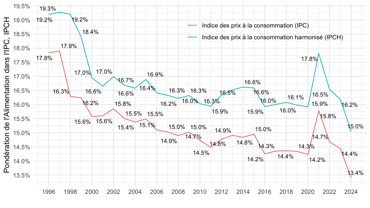
`IPCH-2015` |>
  bind_rows(`IPC-2015`) |>
  filter(COICOP2016 %in% c("01"),
         NATURE == "POND",
         REF_AREA == "FE",
         is.na(MENAGES_IPC) | MENAGES_IPC == "ENSEMBLE") |>
  year_to_date() |>

  group_by(INDICATEUR) |>
  filter(date >= as.Date("2010-01-01")) |>
  arrange(date) |>
  ggplot() + ylab("Pondération de l'Alimentation dans l'IPC, IPCH") + xlab("") + theme_minimal() +
  geom_line(aes(x = date, y = OBS_VALUE/10000, color = Indicateur)) +

  scale_x_date(breaks = seq(1920, 2100, 1) |> paste0("-01-01") |> as.Date(),
               labels = date_format("%Y")) +
  theme(legend.position = c(0.7, 0.85),
        legend.title = element_blank()) +
  scale_y_continuous(breaks = 0.01*seq(0, 300, .5),
                     labels = percent_format(accuracy = .1)) +
  geom_text_repel(aes(x = date, y = OBS_VALUE/10000, label = percent(OBS_VALUE/10000, acc = 0.1)),
                  fontface ="plain", color = "black", size = 3)
`IPCH-2015` |>
  bind_rows(`IPC-2015`) |>
  filter(COICOP2016 %in% c("02"),
         NATURE == "POND",
         REF_AREA == "FE",
         is.na(MENAGES_IPC) | MENAGES_IPC == "ENSEMBLE") |>
  year_to_date() |>

  group_by(INDICATEUR) |>
  filter(date >= as.Date("1996-01-01")) |>
  arrange(date) |>
  ggplot() + ylab("Pondération de l'Alimentation dans l'IPC, IPCH") + xlab("") + theme_minimal() +
  geom_line(aes(x = date, y = OBS_VALUE/10000, color = Indicateur)) +

  scale_x_date(breaks = seq(1920, 2100, 2) |> paste0("-01-01") |> as.Date(),
               labels = date_format("%Y")) +
  theme(legend.position = c(0.7, 0.85),
        legend.title = element_blank()) +
  scale_y_continuous(breaks = 0.01*seq(0, 300, .5),
                     labels = percent_format(accuracy = .1))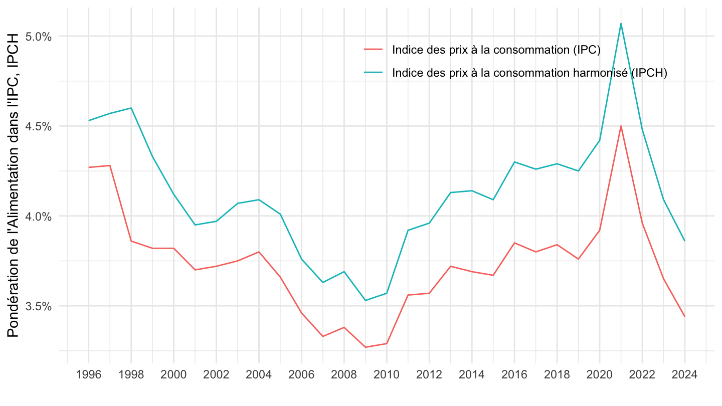
`IPCH-2015` |>
  bind_rows(`IPC-2015`) |>
  filter(COICOP2016 %in% c("11"),
         NATURE == "POND",
         REF_AREA == "FE",
         is.na(MENAGES_IPC) | MENAGES_IPC == "ENSEMBLE") |>
  year_to_date() |>

  group_by(INDICATEUR) |>
  filter(date >= as.Date("1996-01-01")) |>
  arrange(date) |>
  ggplot() + ylab("Pondération dans l'IPC, IPCH") + xlab("") + theme_minimal() +
  geom_line(aes(x = date, y = OBS_VALUE/10000, color = Indicateur)) +

  scale_x_date(breaks = seq(1920, 2100, 2) |> paste0("-01-01") |> as.Date(),
               labels = date_format("%Y")) +
  theme(legend.position = c(0.4, 0.15),
        legend.title = element_blank()) +
  scale_y_continuous(breaks = 0.01*seq(0, 300, .5),
                     labels = percent_format(accuracy = .1))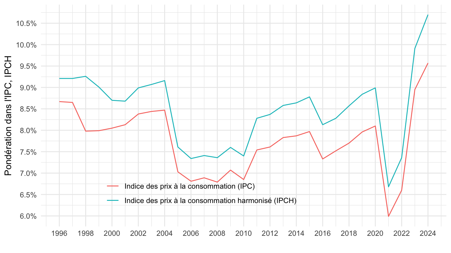
`IPCH-2015` |>
  bind_rows(`IPC-2015`) |>
  filter(COICOP2016 %in% c("1112"),
         NATURE == "POND",
         REF_AREA == "FE",
         is.na(MENAGES_IPC) | MENAGES_IPC == "ENSEMBLE") |>
  year_to_date() |>

  group_by(INDICATEUR) |>
  filter(date >= as.Date("1996-01-01")) |>
  arrange(date) |>
  ggplot() + ylab("Pondération dans l'IPC, IPCH") + xlab("") + theme_minimal() +
  geom_line(aes(x = date, y = OBS_VALUE/10000, color = Indicateur)) +

  scale_x_date(breaks = seq(1920, 2100, 2) |> paste0("-01-01") |> as.Date(),
               labels = date_format("%Y")) +
  theme(legend.position = c(0.4, 0.15),
        legend.title = element_blank()) +
  scale_y_continuous(breaks = 0.01*seq(0, 300, .1),
                     labels = percent_format(accuracy = .1))
`IPCH-2015` |>
  bind_rows(`IPC-2015`) |>
  filter(COICOP2016 %in% c("03"),
         NATURE == "POND",
         REF_AREA == "FE",
         is.na(MENAGES_IPC) | MENAGES_IPC == "ENSEMBLE") |>
  year_to_date() |>

  group_by(INDICATEUR) |>
  filter(date >= as.Date("1996-01-01")) |>
  arrange(date) |>
  ggplot() + ylab("Pondération de l'Habillement dans l'IPC, IPCH") + xlab("") + theme_minimal() +
  geom_line(aes(x = date, y = OBS_VALUE/10000, color = Indicateur)) +

  scale_x_date(breaks = seq(1920, 2100, 2) |> paste0("-01-01") |> as.Date(),
               labels = date_format("%Y")) +
  theme(legend.position = c(0.7, 0.85),
        legend.title = element_blank()) +
  scale_y_continuous(breaks = 0.01*seq(0, 300, .5),
                     labels = percent_format(accuracy = .1))
`IPCH-2015` |>
  bind_rows(`IPC-2015`) |>
  filter(COICOP2016 %in% c("04"),
         NATURE == "POND",
         REF_AREA == "FE",
         is.na(MENAGES_IPC) | MENAGES_IPC == "ENSEMBLE") |>
  year_to_date() |>

  group_by(INDICATEUR) |>
  filter(date >= as.Date("1996-01-01")) |>
  arrange(date) |>
  ggplot() + ylab("Pondération du Logement dans l'IPC, IPCH") + xlab("") + theme_minimal() +
  geom_line(aes(x = date, y = OBS_VALUE/10000, color = Indicateur)) +

  scale_x_date(breaks = seq(1920, 2100, 2) |> paste0("-01-01") |> as.Date(),
               labels = date_format("%Y")) +
  theme(legend.position = c(0.3, 0.85),
        legend.title = element_blank()) +
  scale_y_continuous(breaks = 0.01*seq(0, 300, 1),
                     labels = percent_format(accuracy = 1)) +
  geom_text_repel(aes(x = date, y = OBS_VALUE/10000, label = percent(OBS_VALUE/10000, acc = 0.1)),
                  fontface ="plain", color = "black", size = 3)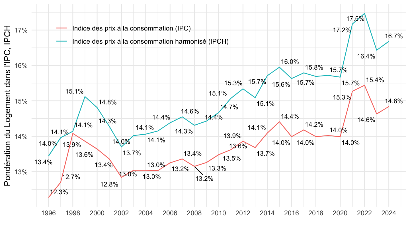
`IPCH-2015` |>
  bind_rows(`IPC-2015`) |>
  filter(COICOP2016 %in% c("041"),
         NATURE == "POND",
         REF_AREA == "FE",
         is.na(MENAGES_IPC) | MENAGES_IPC == "ENSEMBLE") |>
  year_to_date() |>

  group_by(INDICATEUR) |>
  filter(date >= as.Date("1996-01-01")) |>
  arrange(date) |>
  ggplot() + ylab("Pondération des Loyers dans l'IPC, IPCH") + xlab("") + theme_minimal() +
  geom_line(aes(x = date, y = OBS_VALUE/10000, color = Indicateur)) +

  scale_x_date(breaks = seq(1920, 2100, 2) |> paste0("-01-01") |> as.Date(),
               labels = date_format("%Y")) +
  theme(legend.position = c(0.3, 0.85),
        legend.title = element_blank()) +
  scale_y_continuous(breaks = 0.01*seq(0, 300, .2),
                     labels = percent_format(accuracy = .1)) +
  geom_text_repel(aes(x = date, y = OBS_VALUE/10000, label = percent(OBS_VALUE/10000, acc = 0.1)),
                  fontface ="plain", color = "black", size = 3)
`IPCH-2015` |>
  bind_rows(`IPC-2015`) |>
  filter(COICOP2016 %in% c("07"),
         NATURE == "POND",
         REF_AREA == "FE",
         is.na(MENAGES_IPC) | MENAGES_IPC == "ENSEMBLE") |>
  year_to_date() |>

  group_by(INDICATEUR) |>
  filter(date >= as.Date("1996-01-01")) |>
  arrange(date) |>
  ggplot() + ylab("Pondération des Transports dans l'IPC, IPCH") + xlab("") + theme_minimal() +
  geom_line(aes(x = date, y = OBS_VALUE/10000, color = Indicateur)) +

  scale_x_date(breaks = seq(1920, 2100, 2) |> paste0("-01-01") |> as.Date(),
               labels = date_format("%Y")) +
  theme(legend.position = c(0.7, 0.85),
        legend.title = element_blank()) +
  scale_y_continuous(breaks = 0.01*seq(0, 300, .5),
                     labels = percent_format(accuracy = .1))
`IPCH-2015` |>
  bind_rows(`IPC-2015`) |>
  filter(COICOP2016 %in% c("07311"),
         NATURE == "POND",
         REF_AREA == "FE",
         is.na(MENAGES_IPC) | MENAGES_IPC == "ENSEMBLE") |>
  year_to_date() |>

  group_by(INDICATEUR) |>
  filter(date >= as.Date("1996-01-01")) |>
  arrange(date) |>
  ggplot() + ylab("Pondération des Transports dans l'IPC, IPCH") + xlab("") + theme_minimal() +
  geom_line(aes(x = date, y = OBS_VALUE/10000, color = Indicateur)) +

  scale_x_date(breaks = seq(1920, 2100, 2) |> paste0("-01-01") |> as.Date(),
               labels = date_format("%Y")) +
  theme(legend.position = c(0.7, 0.85),
        legend.title = element_blank()) +
  scale_y_continuous(breaks = 0.01*seq(0, 300, .1),
                     labels = percent_format(accuracy = .1))
`IPCH-2015` |>
  bind_rows(`IPC-2015`) |>
  filter(COICOP2016 %in% c("0711"),
         NATURE == "POND",
         REF_AREA == "FE",
         is.na(MENAGES_IPC) | MENAGES_IPC == "ENSEMBLE") |>
  year_to_date() |>

  group_by(INDICATEUR) |>
  filter(date >= as.Date("1996-01-01")) |>
  arrange(date) |>
  ggplot() + ylab("Pondération des Transports dans l'IPC, IPCH") + xlab("") + theme_minimal() +
  geom_line(aes(x = date, y = OBS_VALUE/10000, color = Indicateur)) +

  scale_x_date(breaks = seq(1920, 2100, 2) |> paste0("-01-01") |> as.Date(),
               labels = date_format("%Y")) +
  theme(legend.position = c(0.7, 0.85),
        legend.title = element_blank()) +
  scale_y_continuous(breaks = 0.01*seq(0, 300, .1),
                     labels = percent_format(accuracy = .1))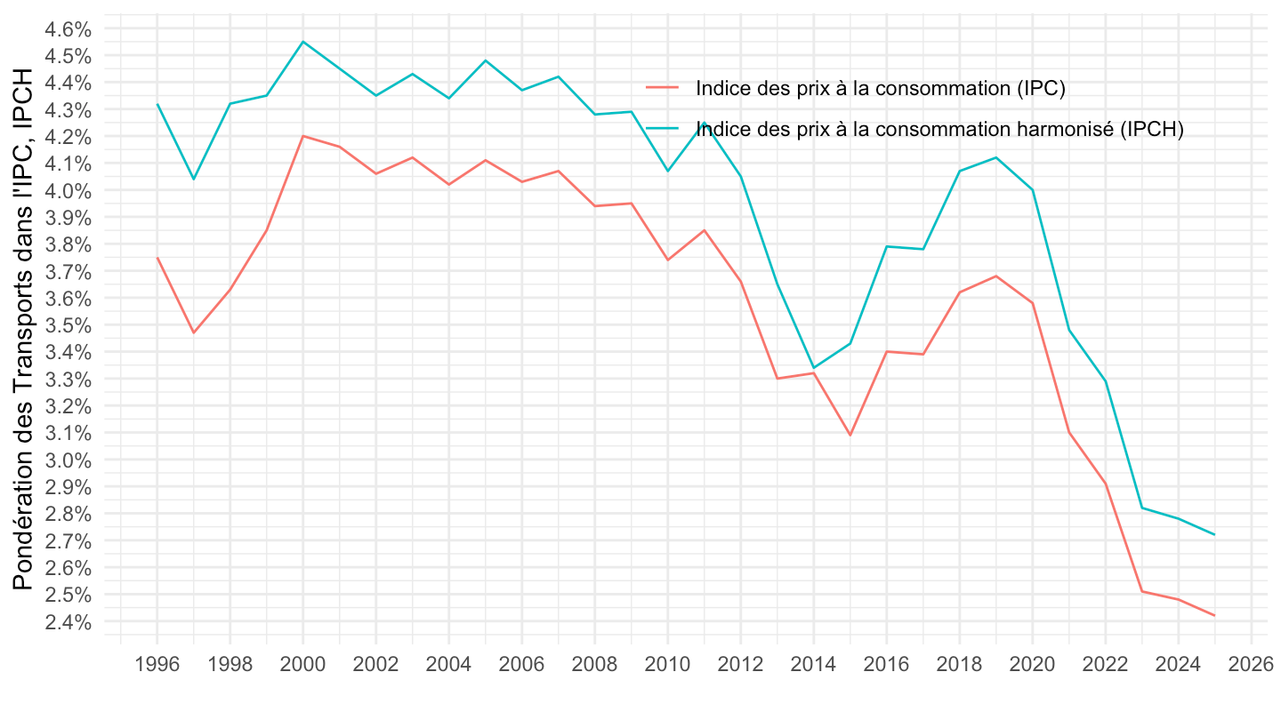
`IPCH-2015` |>
  bind_rows(`IPC-2015`) |>
  filter(COICOP2016 %in% c("0712"),
         NATURE == "POND",
         REF_AREA == "FE",
         is.na(MENAGES_IPC) | MENAGES_IPC == "ENSEMBLE") |>
  year_to_date() |>

  group_by(INDICATEUR) |>
  filter(date >= as.Date("1996-01-01")) |>
  arrange(date) |>
  ggplot() + ylab("Pondération des Transports dans l'IPC, IPCH") + xlab("") + theme_minimal() +
  geom_line(aes(x = date, y = OBS_VALUE/10000, color = Indicateur)) +

  scale_x_date(breaks = seq(1920, 2100, 2) |> paste0("-01-01") |> as.Date(),
               labels = date_format("%Y")) +
  theme(legend.position = c(0.7, 0.85),
        legend.title = element_blank()) +
  scale_y_continuous(breaks = 0.01*seq(0, 300, .1),
                     labels = percent_format(accuracy = .1))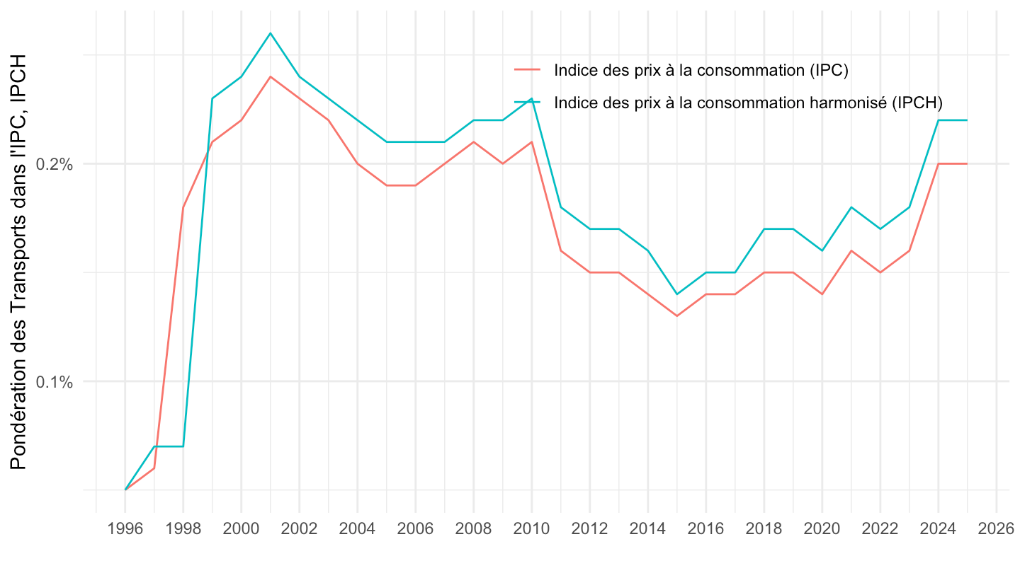
`IPCH-2015` |>
  bind_rows(`IPC-2015`) |>
  filter(COICOP2016 %in% c("08"),
         NATURE == "POND",
         REF_AREA == "FE",
         is.na(MENAGES_IPC) | MENAGES_IPC == "ENSEMBLE") |>
  year_to_date() |>

  group_by(INDICATEUR) |>
  filter(date >= as.Date("1996-01-01")) |>
  arrange(date) |>
  ggplot() + ylab("Pondération des Communications dans l'IPC, IPCH") + xlab("") + theme_minimal() +
  geom_line(aes(x = date, y = OBS_VALUE/10000, color = Indicateur)) +

  scale_x_date(breaks = seq(1920, 2100, 2) |> paste0("-01-01") |> as.Date(),
               labels = date_format("%Y")) +
  theme(legend.position = c(0.7, 0.2),
        legend.title = element_blank()) +
  scale_y_continuous(breaks = 0.01*seq(0, 300, .2),
                     labels = percent_format(accuracy = .1))
`IPCH-2015` |>
  bind_rows(`IPC-2015`) |>
  filter(COICOP2016 %in% c("12"),
         NATURE == "POND",
         REF_AREA == "FE",
         is.na(MENAGES_IPC) | MENAGES_IPC == "ENSEMBLE") |>
  year_to_date() |>

  group_by(INDICATEUR) |>
  filter(date >= as.Date("1996-01-01")) |>
  arrange(date) |>
  ggplot() + ylab("Pondérationdans l'IPC, IPCH") + xlab("") + theme_minimal() +
  geom_line(aes(x = date, y = OBS_VALUE/10000, color = Indicateur)) +

  scale_x_date(breaks = seq(1920, 2100, 2) |> paste0("-01-01") |> as.Date(),
               labels = date_format("%Y")) +
  theme(legend.position = c(0.7, 0.2),
        legend.title = element_blank()) +
  scale_y_continuous(breaks = 0.01*seq(0, 300, .2),
                     labels = percent_format(accuracy = .1))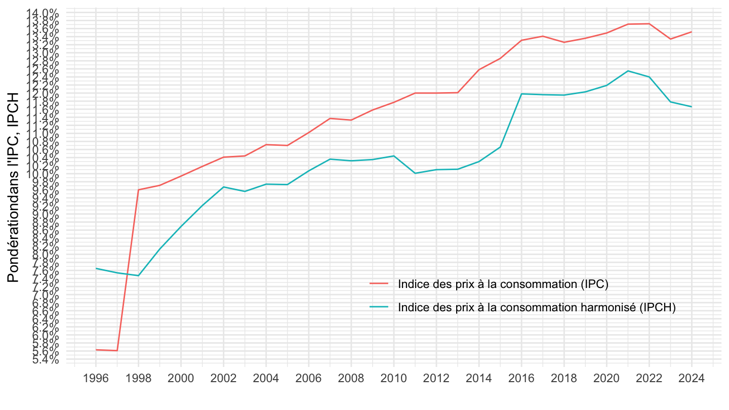
`IPCH-2015` |>
  bind_rows(`IPC-2015`) |>
  filter(COICOP2016 %in% c("124"),
         NATURE == "POND",
         REF_AREA == "FE",
         is.na(MENAGES_IPC) | MENAGES_IPC == "ENSEMBLE") |>
  year_to_date() |>

  group_by(INDICATEUR) |>
  filter(date >= as.Date("1996-01-01")) |>
  arrange(date) |>
  ggplot() + ylab("Pondérationdans l'IPC, IPCH") + xlab("") + theme_minimal() +
  geom_line(aes(x = date, y = OBS_VALUE/10000, color = Indicateur)) +

  scale_x_date(breaks = seq(1920, 2100, 2) |> paste0("-01-01") |> as.Date(),
               labels = date_format("%Y")) +
  theme(legend.position = c(0.7, 0.2),
        legend.title = element_blank()) +
  scale_y_continuous(breaks = 0.01*seq(0, 300, .2),
                     labels = percent_format(accuracy = .1))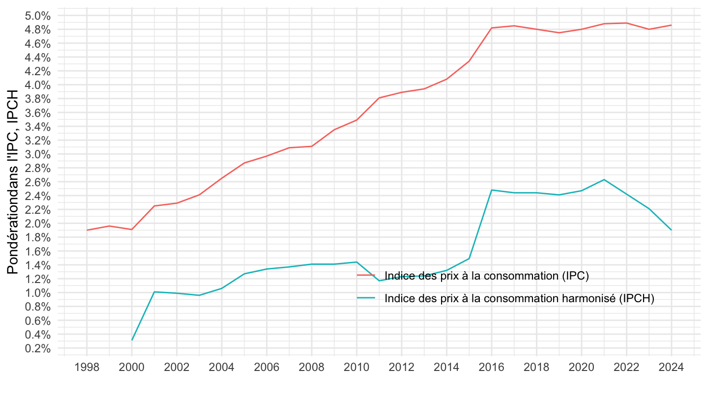
`IPCH-2015` |>
  bind_rows(`IPC-2015`) |>
  filter(COICOP2016 %in% c("12401"),
         NATURE == "POND",
         REF_AREA == "FE",
         is.na(MENAGES_IPC) | MENAGES_IPC == "ENSEMBLE") |>
  year_to_date() |>

  group_by(INDICATEUR) |>
  filter(date >= as.Date("1996-01-01")) |>
  arrange(date) |>
  ggplot() + ylab("Pondérationdans l'IPC, IPCH") + xlab("") + theme_minimal() +
  geom_line(aes(x = date, y = OBS_VALUE/10000, color = Indicateur)) +

  scale_x_date(breaks = seq(1920, 2100, 2) |> paste0("-01-01") |> as.Date(),
               labels = date_format("%Y")) +
  theme(legend.position = c(0.7, 0.2),
        legend.title = element_blank()) +
  scale_y_continuous(breaks = 0.01*seq(0, 300, .2),
                     labels = percent_format(accuracy = .1))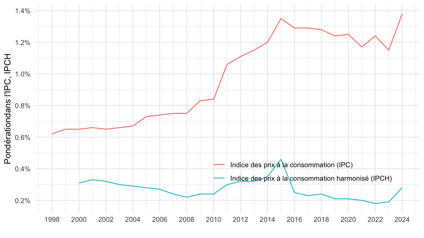
`IPCH-2015` |>
  bind_rows(`IPC-2015`) |>
  filter(COICOP2016 %in% c("12402"),
         NATURE == "POND",
         REF_AREA == "FE",
         is.na(MENAGES_IPC) | MENAGES_IPC == "ENSEMBLE") |>
  year_to_date() |>

  group_by(INDICATEUR) |>
  filter(date >= as.Date("1996-01-01")) |>
  arrange(date) |>
  ggplot() + ylab("Pondérationdans l'IPC, IPCH") + xlab("") + theme_minimal() +
  geom_line(aes(x = date, y = OBS_VALUE/10000, color = Indicateur)) +

  scale_x_date(breaks = seq(1920, 2100, 2) |> paste0("-01-01") |> as.Date(),
               labels = date_format("%Y")) +
  theme(legend.position = c(0.7, 0.2),
        legend.title = element_blank()) +
  scale_y_continuous(breaks = 0.01*seq(0, 300, .2),
                     labels = percent_format(accuracy = .1))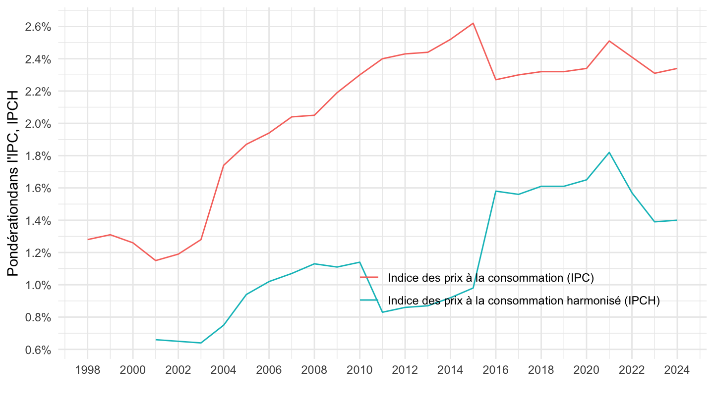
`IPCH-2015` |>
  bind_rows(`IPC-2015`) |>
  filter(COICOP2016 %in% c("12403"),
         NATURE == "POND",
         REF_AREA == "FE",
         is.na(MENAGES_IPC) | MENAGES_IPC == "ENSEMBLE") |>
  year_to_date() |>

  group_by(INDICATEUR) |>
  filter(date >= as.Date("1996-01-01")) |>
  arrange(date) |>
  ggplot() + ylab("Pondération dans l'IPC, IPCH") + xlab("") + theme_minimal() +
  geom_line(aes(x = date, y = OBS_VALUE/10000, color = Indicateur)) +

  scale_x_date(breaks = seq(1920, 2100, 2) |> paste0("-01-01") |> as.Date(),
               labels = date_format("%Y")) +
  theme(legend.position = c(0.7, 0.2),
        legend.title = element_blank()) +
  scale_y_continuous(breaks = 0.01*seq(0, 300, .2),
                     labels = percent_format(accuracy = .1))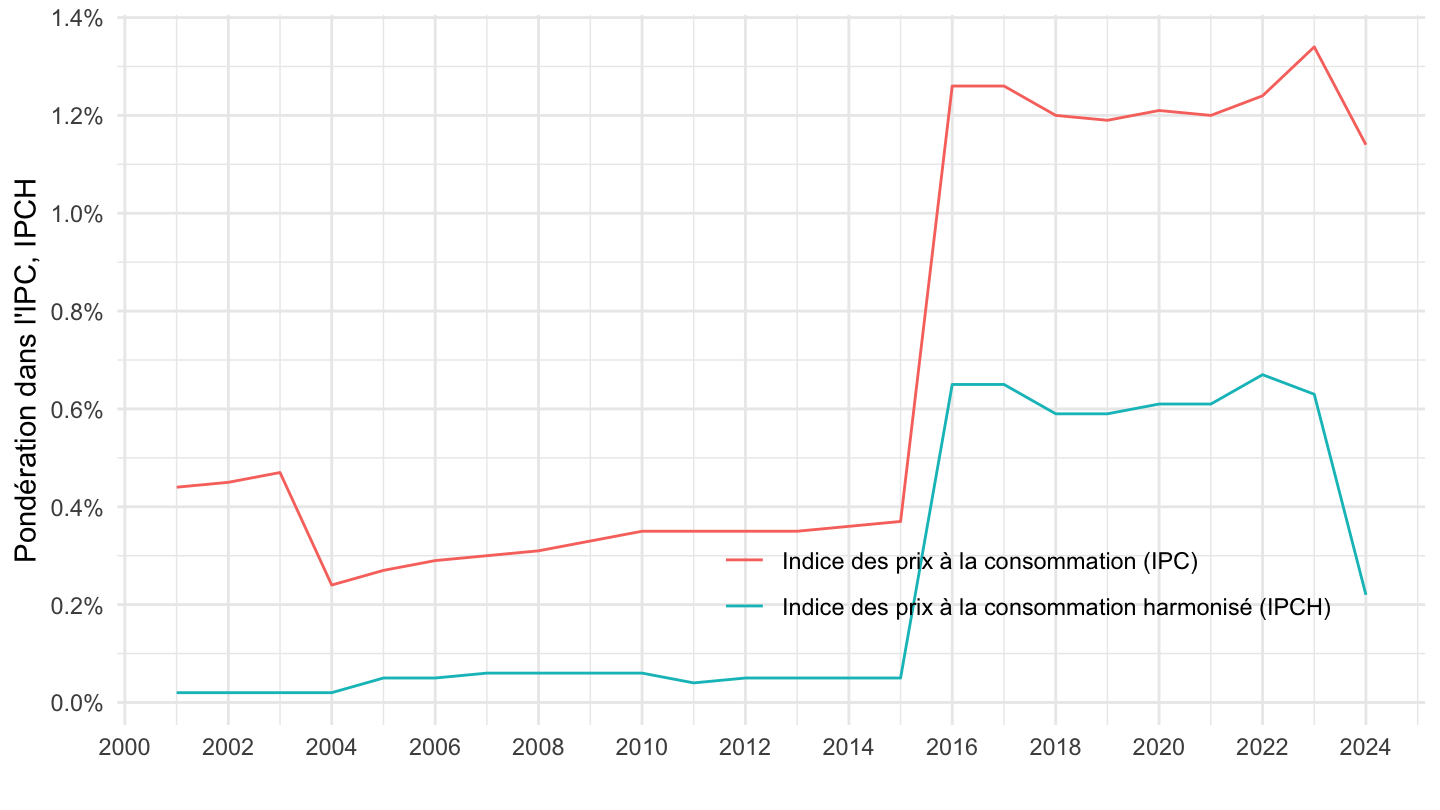
`IPCH-2015` |>
  bind_rows(`IPC-2015`) |>
  filter(IDBANK %in% c("001763082", "001763083", "001763084")) |>
  month_to_date() |>

  group_by(COICOP2016) |>
  filter(date >= as.Date("1996-01-01")) |>
  arrange(date) |>
  mutate(OBS_VALUE = 100*OBS_VALUE/OBS_VALUE[date == as.Date("1996-01-01")]) |>
  ggplot() + ylab("0711 - Voitures automobiles") + xlab("") + theme_minimal() +
  geom_line(aes(x = date, y = OBS_VALUE, color = Coicop2016)) +

  scale_x_date(breaks = seq(1920, 2100, 2) |> paste0("-01-01") |> as.Date(),
               labels = date_format("%Y")) +
  theme(legend.position = c(0.3, 0.8),
        legend.title = element_blank()) +
  scale_y_log10(breaks = seq(10, 300, 5),
                     labels = dollar_format(accuracy = 1, prefix = ""))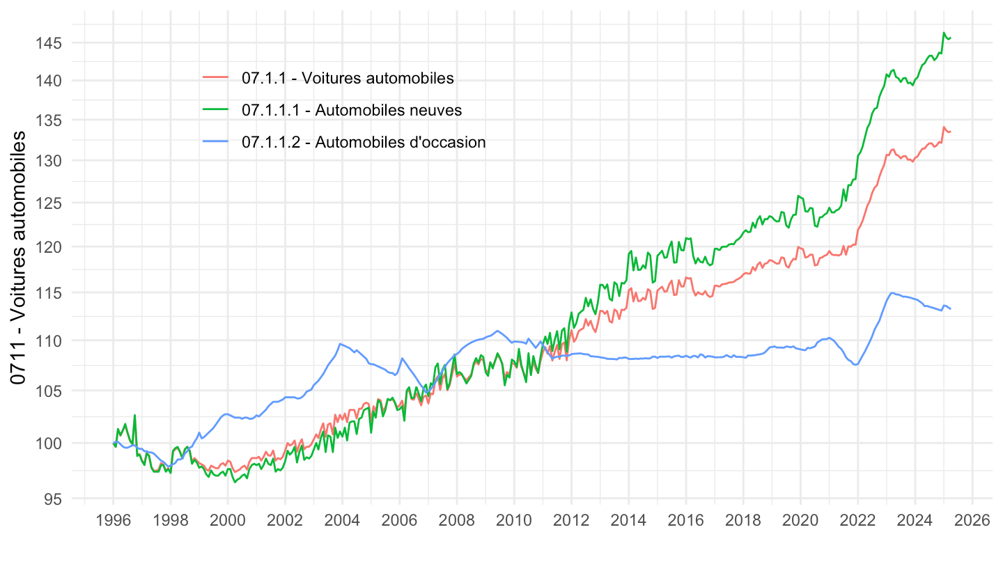
`IPCH-2015` |>
  bind_rows(`IPC-2015`) |>
  filter(IDBANK %in% c("001763082", "001763083", "001763084")) |>
  month_to_date() |>

  group_by(COICOP2016) |>
  filter(date >= as.Date("2017-01-01")) |>
  arrange(date) |>
  mutate(OBS_VALUE = 100*OBS_VALUE/OBS_VALUE[date == as.Date("2017-01-01")]) |>
  ggplot() + ylab("0711 - Voitures automobiles") + xlab("") + theme_minimal() +
  geom_line(aes(x = date, y = OBS_VALUE, color = Coicop2016)) +

  scale_x_date(breaks = seq(1920, 2100, 1) |> paste0("-01-01") |> as.Date(),
               labels = date_format("%Y")) +
  theme(legend.position = c(0.3, 0.8),
        legend.title = element_blank()) +
  scale_y_log10(breaks = seq(10, 300, 5),
                     labels = dollar_format(accuracy = 1, prefix = ""))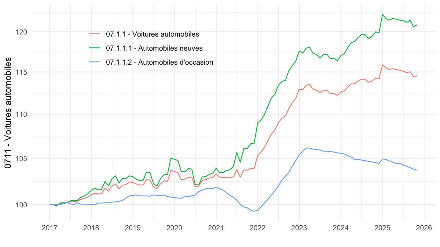
`IPCH-2015` |>
  bind_rows(`IPC-2015`) |>
  filter(IDBANK %in% c("001763082", "001763083", "001763084")) |>
  month_to_date() |>

  group_by(COICOP2016) |>
  filter(date >= as.Date("2019-01-01")) |>
  arrange(date) |>
  mutate(OBS_VALUE = 100*OBS_VALUE/OBS_VALUE[date == as.Date("2019-01-01")]) |>
  ggplot() + ylab("0711 - Voitures automobiles") + xlab("") + theme_minimal() +
  geom_line(aes(x = date, y = OBS_VALUE, color = Coicop2016)) +

  scale_x_date(breaks = seq(1920, 2100, 1) |> paste0("-01-01") |> as.Date(),
               labels = date_format("%Y")) +
  theme(legend.position = c(0.3, 0.8),
        legend.title = element_blank()) +
  scale_y_log10(breaks = seq(10, 300, 5),
                     labels = dollar_format(accuracy = 1, prefix = ""))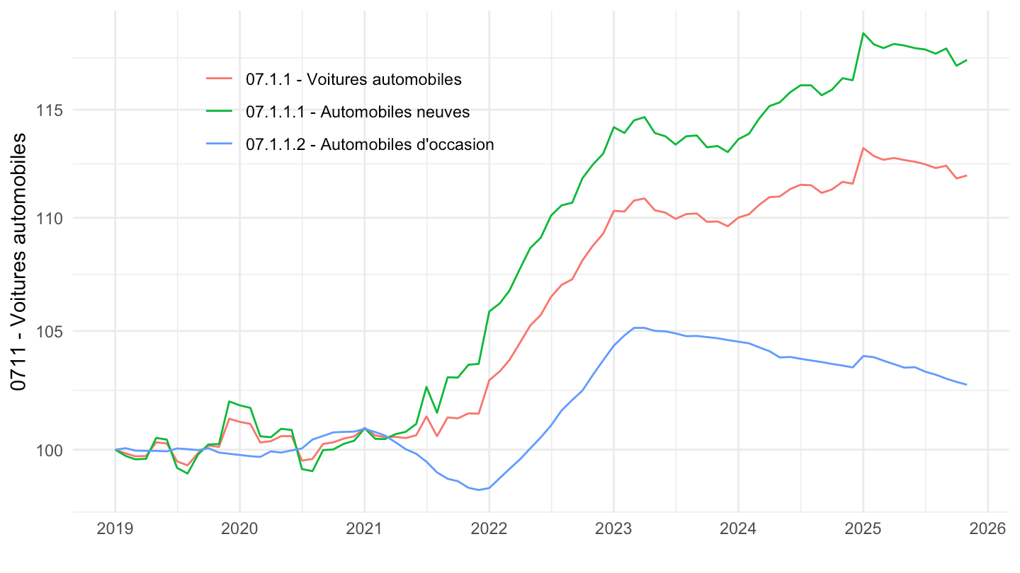
La principale différence entre l’IPCH et l’IPC porte sur les dépenses de santé : l’IPCH suit des prix nets des remboursements de la sécurité sociale tandis que l’IPC suit des prix bruts.
plot_sante <- `IPCH-2015` |>
  bind_rows(`IPC-2015`) |>
  filter(COICOP2016 %in% c("06"),
         NATURE == "INDICE",
         REF_AREA == "FE",
         FREQ == "M",
         is.na(MENAGES_IPC) | MENAGES_IPC == "ENSEMBLE") |>
  month_to_date() |>

  group_by(INDICATEUR) |>
  filter(date >= as.Date("1996-01-01")) |>
  arrange(date) |>
  mutate(OBS_VALUE = 100*OBS_VALUE/OBS_VALUE[date == as.Date("1996-01-01")]) |>
  ggplot() + ylab("Indice de prix - Santé (100 = 1996)") + xlab("") + theme_minimal() +
  geom_line(aes(x = date, y = OBS_VALUE, color = Indicateur)) +

  scale_x_date(breaks = seq(1920, 2100, 2) |> paste0("-01-01") |> as.Date(),
               labels = date_format("%Y")) +
  theme(legend.position = c(0.7, 0.55),
        legend.title = element_blank(),
        axis.text.x = element_text(angle = 45, vjust = 1, hjust = 1)) +
  scale_y_log10(breaks = seq(10, 300, 5),
                     labels = dollar_format(accuracy = 1, prefix = ""))

plot_sante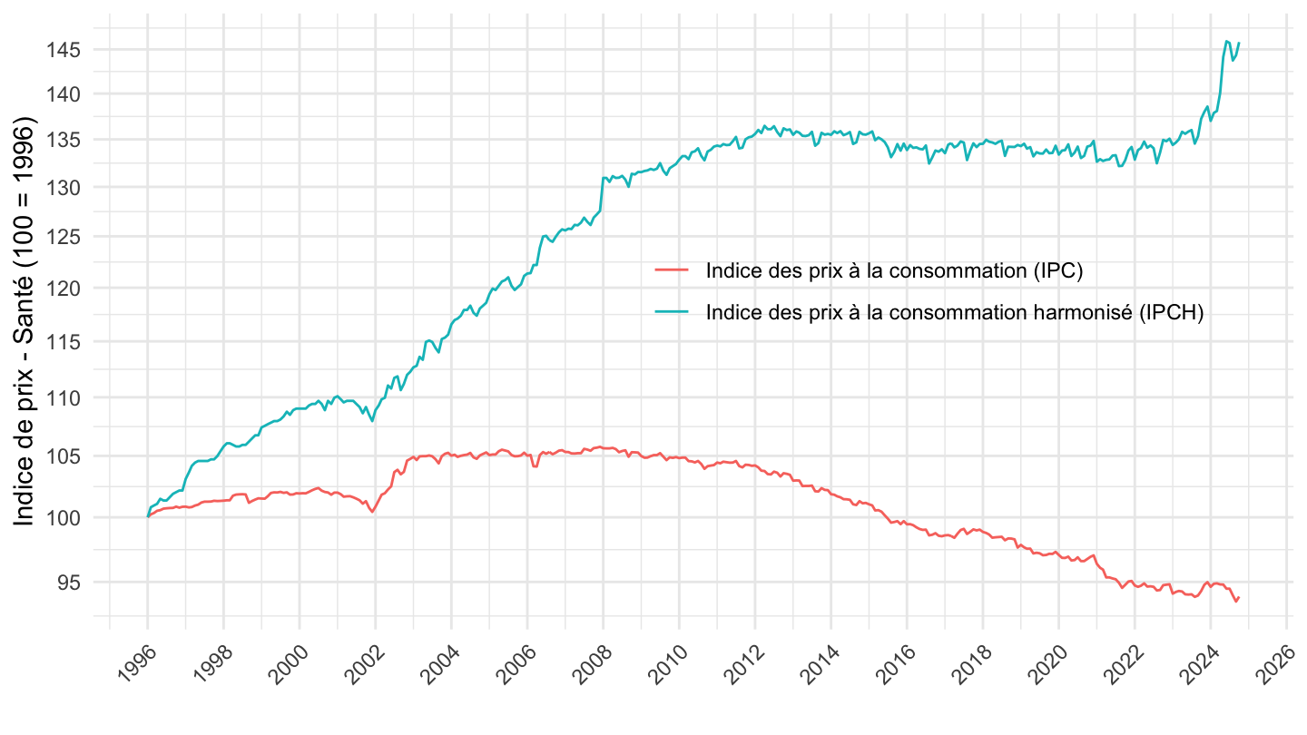
`IPCH-2015` |>
  bind_rows(`IPC-2015`) |>
  filter(COICOP2016 %in% c("06"),
         NATURE == "INDICE",
         REF_AREA == "FE",
         FREQ == "M",
         is.na(MENAGES_IPC) | MENAGES_IPC == "ENSEMBLE") |>
  month_to_date() |>

  group_by(INDICATEUR) |>
  filter(date >= as.Date("2000-01-01"),
         date <= as.Date("2024-12-01")) |>
  arrange(date) |>
  mutate(OBS_VALUE = 100*OBS_VALUE/OBS_VALUE[date == as.Date("2000-01-01")]) |>
  ggplot() + ylab("Indice de prix - Santé (100 = 2000)") + xlab("") + theme_minimal() +
  geom_line(aes(x = date, y = OBS_VALUE, color = Indicateur)) +

  scale_x_date(breaks = seq(1920, 2100, 2) |> paste0("-01-01") |> as.Date(),
               labels = date_format("%Y")) +
  theme(legend.position = c(0.7, 0.55),
        legend.title = element_blank(),
        axis.text.x = element_text(angle = 45, vjust = 1, hjust = 1)) +
  scale_y_log10(breaks = seq(10, 300, 5),
                     labels = dollar_format(accuracy = 1, prefix = "")) +
  geom_label(data = . %>% filter(date == max(date)), aes(x = date, y = OBS_VALUE, color = Indicateur, label = round(OBS_VALUE, 1)))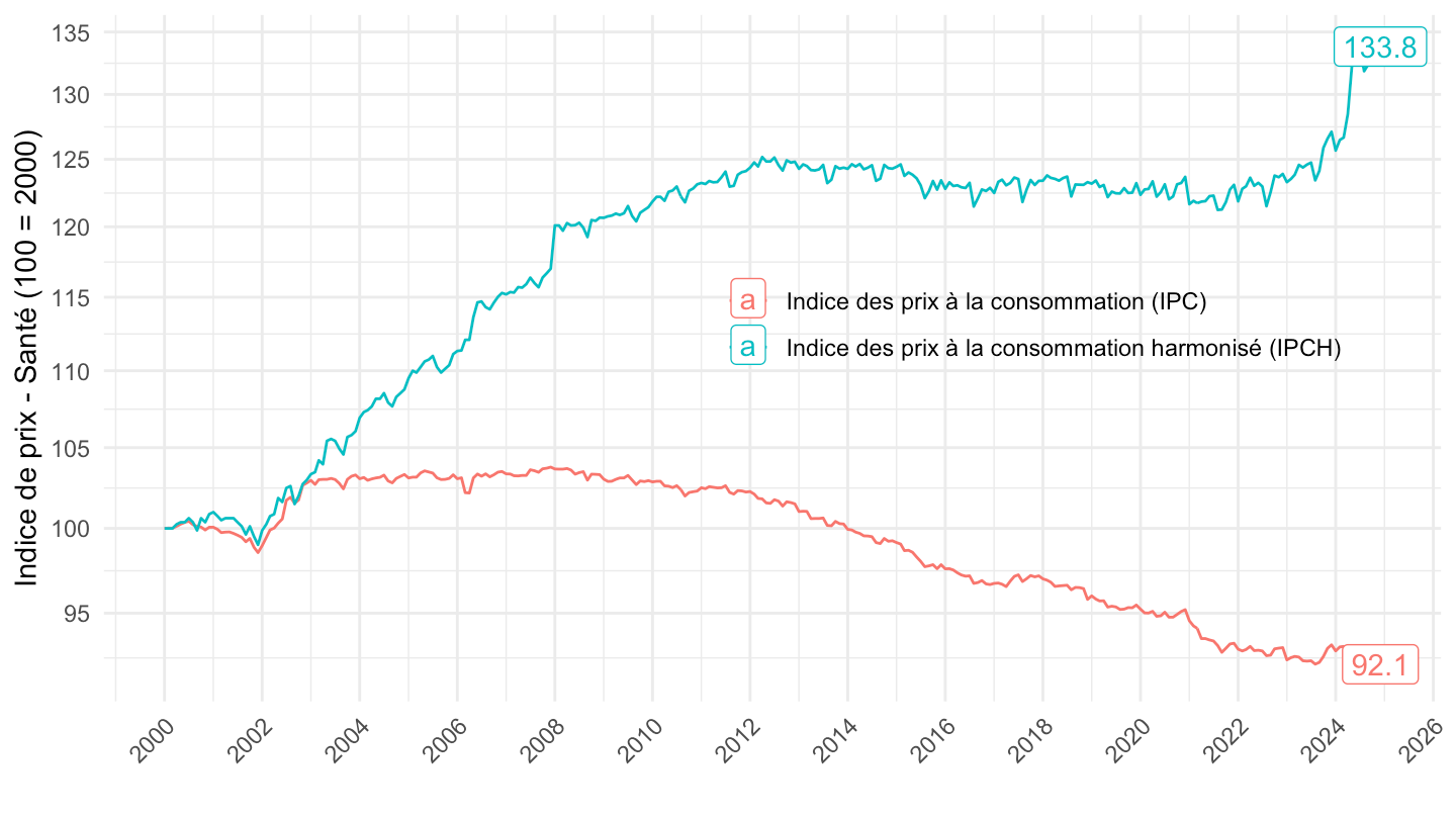
`IPCH-2015` |>
  bind_rows(`IPC-2015`) |>
  filter(COICOP2016 %in% c("06"),
         NATURE == "INDICE",
         REF_AREA == "FE",
         FREQ == "A",
         is.na(MENAGES_IPC) | MENAGES_IPC == "ENSEMBLE") |>
  year_to_date() |>

  group_by(INDICATEUR) |>
  filter(date >= as.Date("2000-01-01"),
         date <= as.Date("2024-12-01")) |>
  arrange(date) |>
  mutate(OBS_VALUE = 100*OBS_VALUE/OBS_VALUE[date == as.Date("2000-01-01")]) |>
  ggplot() + ylab("Indice de prix - Santé (100 = 2000)") + xlab("") + theme_minimal() +
  geom_line(aes(x = date, y = OBS_VALUE, color = Indicateur)) +

  scale_x_date(breaks = seq(1920, 2100, 2) |> paste0("-01-01") |> as.Date(),
               labels = date_format("%Y")) +
  theme(legend.position = c(0.7, 0.55),
        legend.title = element_blank(),
        axis.text.x = element_text(angle = 45, vjust = 1, hjust = 1)) +
  scale_y_log10(breaks = seq(10, 300, 5),
                     labels = dollar_format(accuracy = 1, prefix = "")) +
  geom_label(data = . %>% filter(date == max(date)), aes(x = date, y = OBS_VALUE, color = Indicateur, label = round(OBS_VALUE, 1)))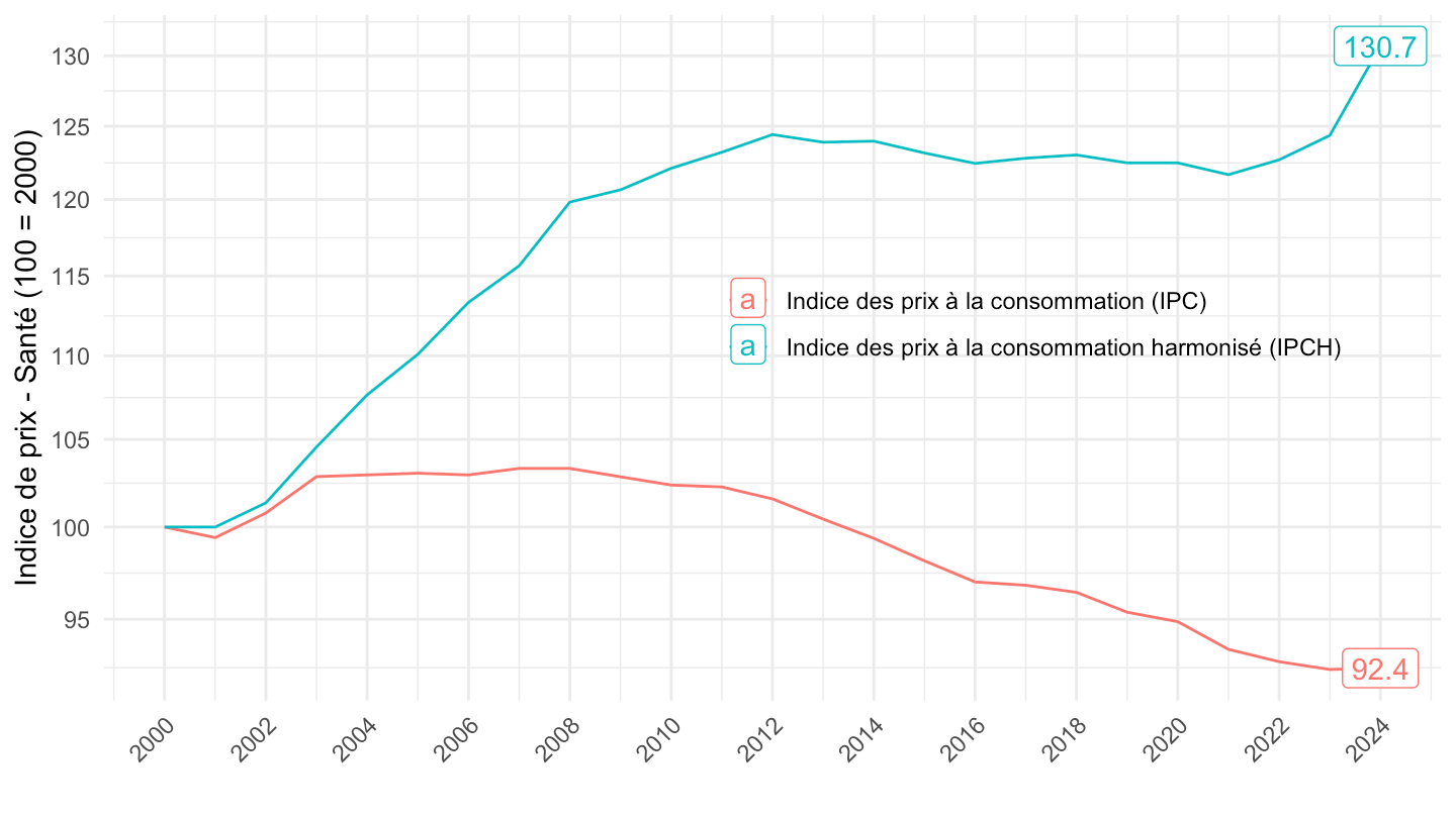
ggarrange(plot_sante_ponderation, plot_sante, common.legend = T)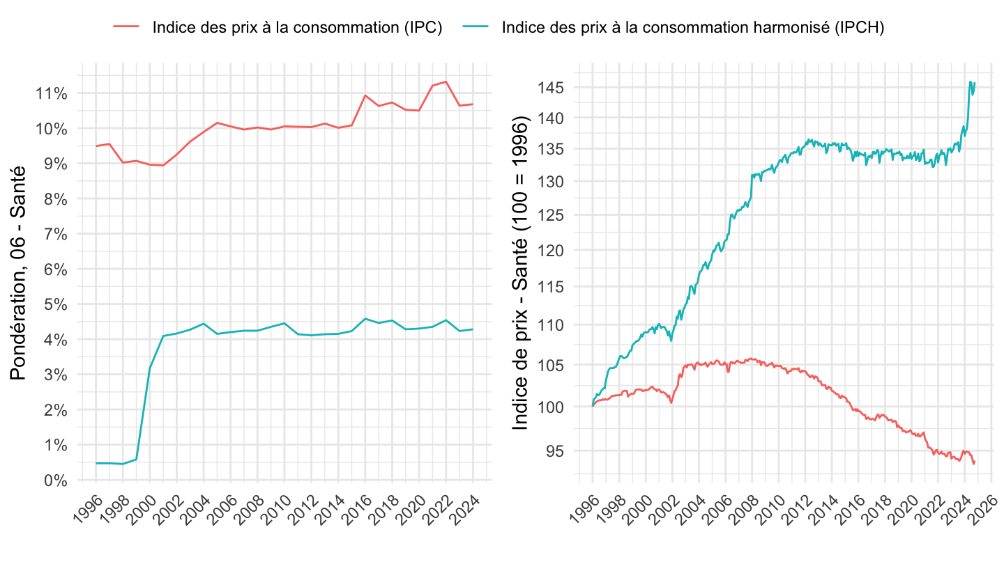
`IPCH-2015` |>
  bind_rows(`IPC-2015`) |>
  filter(COICOP2016 %in% c("06"),
         NATURE == "INDICE",
         REF_AREA == "FE",
         FREQ == "M",
         is.na(MENAGES_IPC) | MENAGES_IPC == "ENSEMBLE") |>
  month_to_date() |>

  group_by(INDICATEUR) |>
  filter(date >= as.Date("2018-01-01")) |>
  arrange(date) |>
  mutate(OBS_VALUE = 100*OBS_VALUE/OBS_VALUE[date == as.Date("2018-01-01")]) |>
  ggplot() + ylab("06 - Santé") + xlab("") + theme_minimal() +
  geom_line(aes(x = date, y = OBS_VALUE, color = Indicateur)) +

  scale_x_date(breaks = seq(1920, 2100, 1) |> paste0("-01-01") |> as.Date(),
               labels = date_format("%Y")) +
  theme(legend.position = c(0.4, 0.2),
        legend.title = element_blank()) +
  scale_y_log10(breaks = seq(10, 300, 1),
                     labels = dollar_format(accuracy = 1, prefix = ""))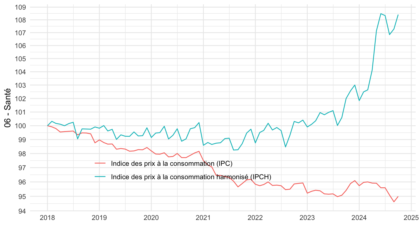
`IPCH-2015` |>
  bind_rows(`IPC-2015`) |>
  filter(COICOP2016 %in% c("06"),
         NATURE == "INDICE",
         REF_AREA == "FE",
         FREQ == "M",
         is.na(MENAGES_IPC) | MENAGES_IPC == "ENSEMBLE") |>
  month_to_date() |>

  group_by(INDICATEUR) |>
  filter(date >= as.Date("2020-01-01")) |>
  arrange(date) |>
  mutate(OBS_VALUE = 100*OBS_VALUE/OBS_VALUE[date == as.Date("2020-01-01")]) |>
  ggplot() + ylab("06 - Santé") + xlab("") + theme_minimal() +
  geom_line(aes(x = date, y = OBS_VALUE, color = Indicateur)) +

  scale_x_date(breaks = seq.Date(as.Date("2019-12-01"), Sys.Date(), "3 months"),
               labels = date_format("%b %Y")) +
  theme(legend.position = c(0.4, 0.2),
        legend.title = element_blank()) +
  scale_y_log10(breaks = seq(10, 300, 1),
                     labels = dollar_format(accuracy = 1, prefix = ""))
`IPCH-2015` |>
  bind_rows(`IPC-2015`) |>
  filter(COICOP2016 %in% c("061"),
         NATURE == "INDICE",
         REF_AREA == "FE",
         FREQ == "M",
         is.na(MENAGES_IPC) | MENAGES_IPC == "ENSEMBLE") |>
  month_to_date() |>

  group_by(INDICATEUR) |>
  filter(date >= as.Date("1996-01-01")) |>
  arrange(date) |>
  mutate(OBS_VALUE = 100*OBS_VALUE/OBS_VALUE[date == as.Date("1996-01-01")]) |>
  ggplot() + ylab("061 - Produits, appareils et matériels médicaux") + xlab("") + theme_minimal() +
  geom_line(aes(x = date, y = OBS_VALUE, color = Indicateur)) +

  scale_x_date(breaks = seq(1920, 2100, 2) |> paste0("-01-01") |> as.Date(),
               labels = date_format("%Y")) +
  theme(legend.position = c(0.7, 0.55),
        legend.title = element_blank()) +
  scale_y_log10(breaks = seq(10, 300, 5),
                     labels = dollar_format(accuracy = 1, prefix = ""))
`IPCH-2015` |>
  bind_rows(`IPC-2015`) |>
  filter(COICOP2016 %in% c("061"),
         NATURE == "INDICE",
         REF_AREA == "FE",
         FREQ == "M",
         is.na(MENAGES_IPC) | MENAGES_IPC == "ENSEMBLE") |>
  month_to_date() |>

  group_by(INDICATEUR) |>
  filter(date >= as.Date("2018-01-01")) |>
  arrange(date) |>
  mutate(OBS_VALUE = 100*OBS_VALUE/OBS_VALUE[date == as.Date("2018-01-01")]) |>
  ggplot() + ylab("061 - Produits, appareils et matériels médicaux") + xlab("") + theme_minimal() +
  geom_line(aes(x = date, y = OBS_VALUE, color = Indicateur)) +

  scale_x_date(breaks = seq(1920, 2100, 1) |> paste0("-01-01") |> as.Date(),
               labels = date_format("%Y")) +
  theme(legend.position = c(0.3, 0.2),
        legend.title = element_blank()) +
  scale_y_log10(breaks = seq(10, 300, 1),
                     labels = dollar_format(accuracy = 1, prefix = ""))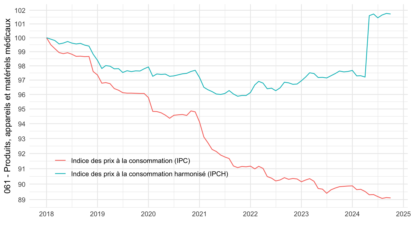
`IPCH-2015` |>
  bind_rows(`IPC-2015`) |>
  filter(COICOP2016 %in% c("061"),
         NATURE == "INDICE",
         REF_AREA == "FE",
         FREQ == "M",
         is.na(MENAGES_IPC) | MENAGES_IPC == "ENSEMBLE") |>
  month_to_date() |>

  group_by(INDICATEUR) |>
  filter(date >= as.Date("2020-01-01")) |>
  arrange(date) |>
  mutate(OBS_VALUE = 100*OBS_VALUE/OBS_VALUE[date == as.Date("2020-01-01")]) |>
  ggplot() + ylab("061 - Produits, appareils et matériels médicaux") + xlab("") + theme_minimal() +
  geom_line(aes(x = date, y = OBS_VALUE, color = Indicateur)) +

  scale_x_date(breaks = seq.Date(as.Date("2019-12-01"), Sys.Date(), "3 months"),
               labels = date_format("%b %Y")) +
  theme(legend.position = c(0.3, 0.2),
        legend.title = element_blank()) +
  scale_y_log10(breaks = seq(10, 300, 1),
                     labels = dollar_format(accuracy = 1, prefix = ""))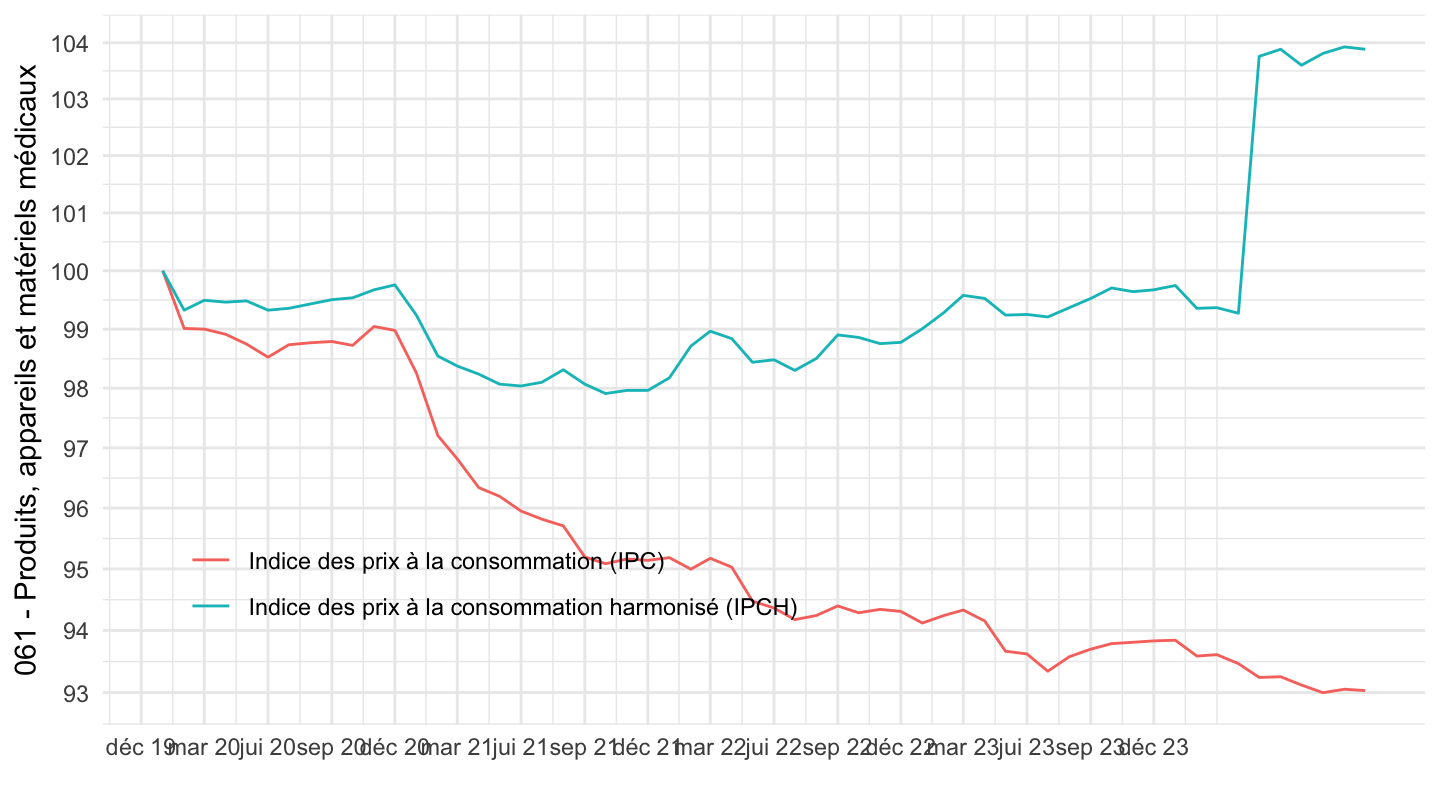
`IPCH-2015` |>
  bind_rows(`IPC-2015`) |>
  filter(COICOP2016 %in% c("062"),
         NATURE == "INDICE",
         REF_AREA == "FE",
         FREQ == "M",
         is.na(MENAGES_IPC) | MENAGES_IPC == "ENSEMBLE") |>
  month_to_date() |>

  group_by(INDICATEUR) |>
  filter(date >= as.Date("1996-01-01")) |>
  arrange(date) |>
  mutate(OBS_VALUE = 100*OBS_VALUE/OBS_VALUE[date == as.Date("2000-01-01")]) |>
  ggplot() + ylab("Indice des prix de la Santé") + xlab("") + theme_minimal() +
  geom_line(aes(x = date, y = OBS_VALUE, color = Indicateur)) +

  scale_x_date(breaks = seq(1920, 2100, 2) |> paste0("-01-01") |> as.Date(),
               labels = date_format("%Y")) +
  theme(legend.position = c(0.7, 0.55),
        legend.title = element_blank()) +
  scale_y_log10(breaks = seq(10, 300, 5),
                     labels = dollar_format(accuracy = 1, prefix = ""))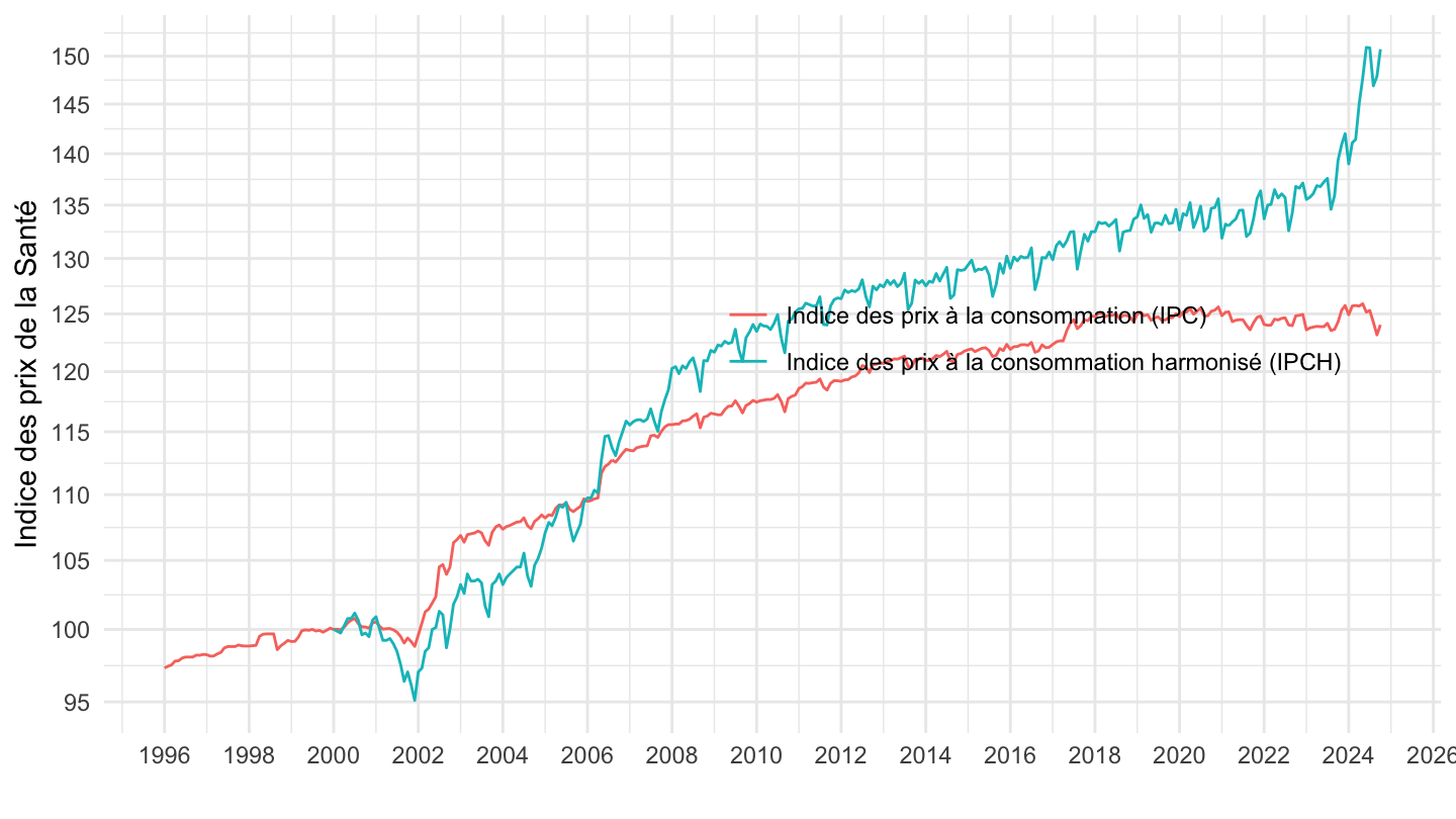
`IPCH-2015` |>
  bind_rows(`IPC-2015`) |>
  filter(COICOP2016 %in% c("0611"),
         NATURE == "INDICE",
         REF_AREA == "FE",
         FREQ == "M",
         is.na(MENAGES_IPC) | MENAGES_IPC == "ENSEMBLE") |>
  month_to_date() |>

  group_by(INDICATEUR) |>
  filter(date >= as.Date("1996-01-01")) |>
  arrange(date) |>
  mutate(OBS_VALUE = 100*OBS_VALUE/OBS_VALUE[date == as.Date("1996-01-01")]) |>
  ggplot() + ylab("0611 - Produits pharmaceutiques") + xlab("") + theme_minimal() +
  geom_line(aes(x = date, y = OBS_VALUE, color = Indicateur)) +

  scale_x_date(breaks = seq(1920, 2100, 2) |> paste0("-01-01") |> as.Date(),
               labels = date_format("%Y")) +
  theme(legend.position = c(0.7, 0.55),
        legend.title = element_blank()) +
  scale_y_log10(breaks = seq(10, 300, 5),
                     labels = dollar_format(accuracy = 1, prefix = ""))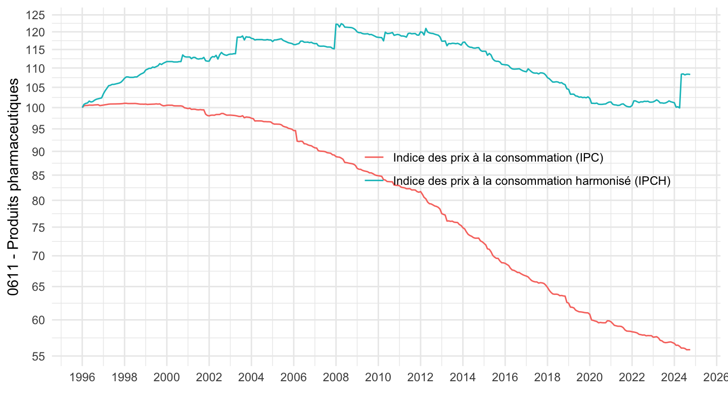
`IPCH-2015` |>
  bind_rows(`IPC-2015`) |>
  filter(COICOP2016 %in% c("0611"),
         NATURE == "INDICE",
         REF_AREA == "FE",
         FREQ == "M",
         is.na(MENAGES_IPC) | MENAGES_IPC == "ENSEMBLE") |>
  month_to_date() |>

  group_by(INDICATEUR) |>
  filter(date >= as.Date("2018-01-01")) |>
  arrange(date) |>
  mutate(OBS_VALUE = 100*OBS_VALUE/OBS_VALUE[date == as.Date("2018-01-01")]) |>
  ggplot() + ylab("0611 - Produits pharmaceutiques") + xlab("") + theme_minimal() +
  geom_line(aes(x = date, y = OBS_VALUE, color = Indicateur)) +

  scale_x_date(breaks = seq(1920, 2100, 1) |> paste0("-01-01") |> as.Date(),
               labels = date_format("%Y")) +
  theme(legend.position = c(0.7, 0.8),
        legend.title = element_blank()) +
  scale_y_log10(breaks = seq(10, 300, 1),
                     labels = dollar_format(accuracy = 1, prefix = ""))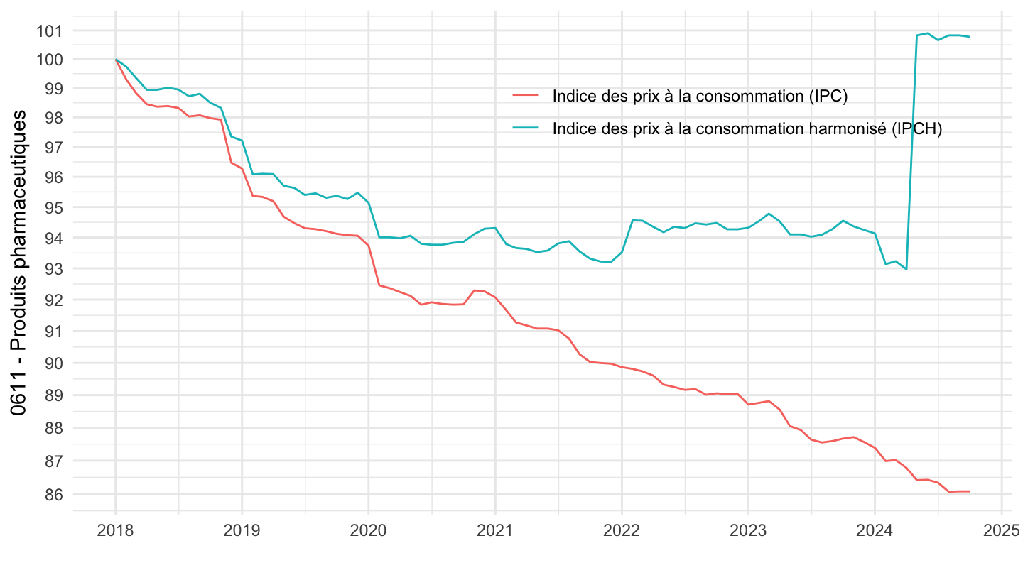
À compter du 15 mai 2024, le montant de la participation forfaitaire passe de 1€ à 2€
`IPCH-2015` |>
  bind_rows(`IPC-2015`) |>
  filter(COICOP2016 %in% c("0611"),
         NATURE == "INDICE",
         REF_AREA == "FE",
         FREQ == "M",
         is.na(MENAGES_IPC) | MENAGES_IPC == "ENSEMBLE") |>
  month_to_date() |>

  group_by(INDICATEUR) |>
  filter(date >= as.Date("2020-01-01")) |>
  arrange(date) |>
  mutate(OBS_VALUE = 100*OBS_VALUE/OBS_VALUE[date == as.Date("2020-01-01")]) |>
  ggplot() + ylab("0611 - Produits pharmaceutiques") + xlab("") + theme_minimal() +
  geom_line(aes(x = date, y = OBS_VALUE, color = Indicateur)) +

  scale_x_date(breaks = seq.Date(as.Date("2019-12-01"), Sys.Date(), "3 months"),
               labels = date_format("%b %Y")) +
  theme(legend.position = c(0.5, 0.9),
        legend.title = element_blank(),
        axis.text.x = element_text(angle = 45, vjust = 1, hjust = 1)) +
  scale_y_log10(breaks = seq(10, 300, 1),
                     labels = dollar_format(accuracy = 1, prefix = ""))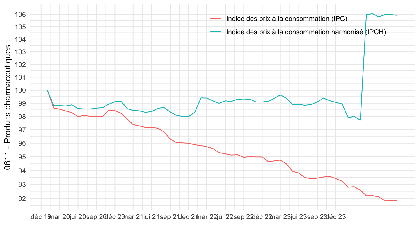
`IPCH-2015` |>
  bind_rows(`IPC-2015`) |>
  filter(COICOP2016 %in% c("0612"),
         NATURE == "INDICE",
         REF_AREA == "FE",
         FREQ == "M",
         is.na(MENAGES_IPC) | MENAGES_IPC == "ENSEMBLE") |>
  month_to_date() |>

  group_by(INDICATEUR) |>
  filter(date >= as.Date("1996-01-01")) |>
  arrange(date) |>
  mutate(OBS_VALUE = 100*OBS_VALUE/OBS_VALUE[date == as.Date("1996-01-01")]) |>
  ggplot() + ylab("0612 - Indice des prix des produits médicaux divers") + xlab("") + theme_minimal() +
  geom_line(aes(x = date, y = OBS_VALUE, color = paste0(Indicateur, "- Produits médicaux divers"))) +

  scale_x_date(breaks = seq(1920, 2100, 2) |> paste0("-01-01") |> as.Date(),
               labels = date_format("%Y")) +
  theme(legend.position = c(0.4, 0.25),
        legend.title = element_blank()) +
  scale_y_log10(breaks = seq(10, 300, 5),
                     labels = dollar_format(accuracy = 1, prefix = ""))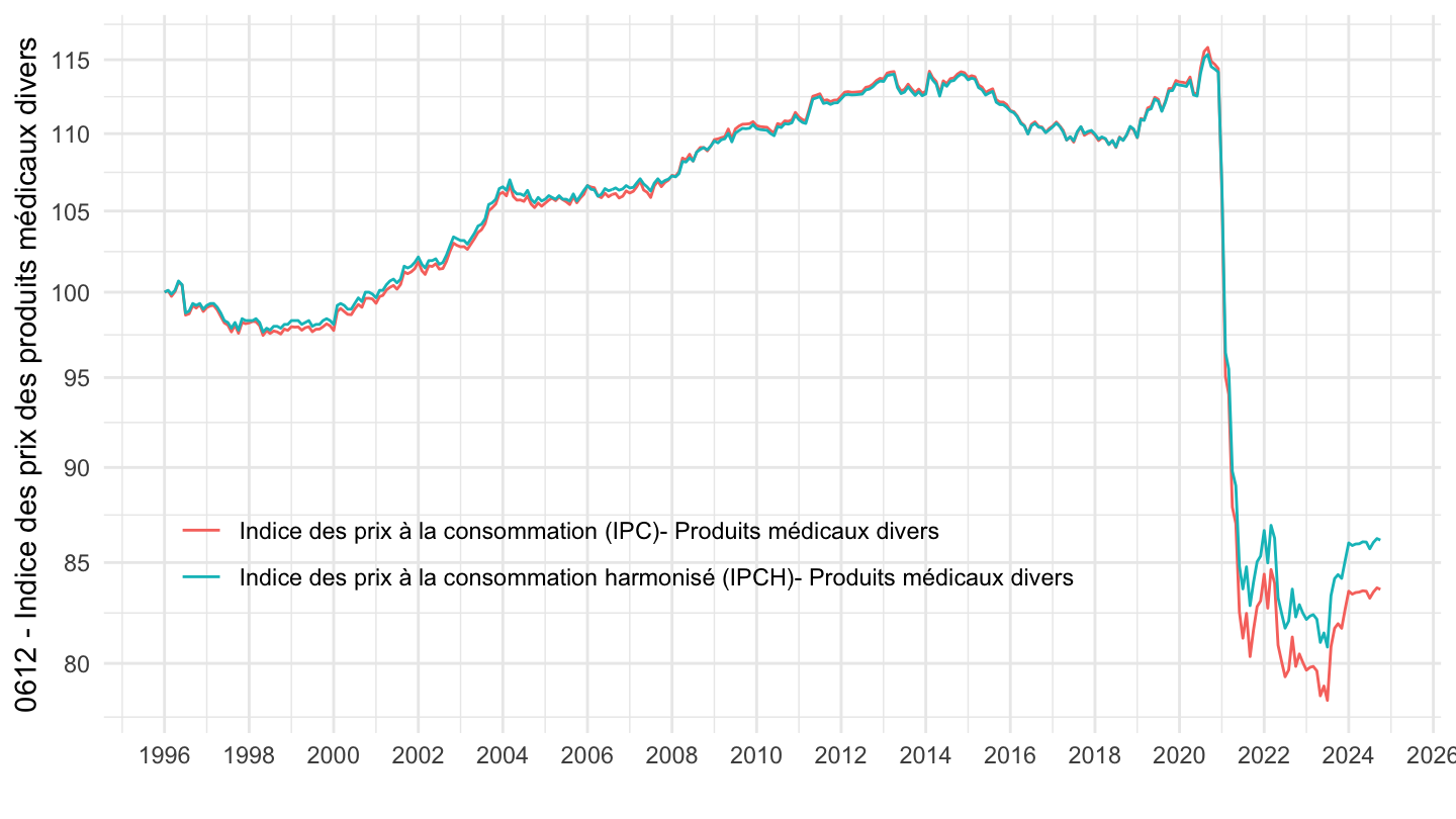
`IPCH-2015` |>
  bind_rows(`IPC-2015`) |>
  filter(COICOP2016 %in% c("0612"),
         NATURE == "INDICE",
         REF_AREA == "FE",
         FREQ == "M",
         is.na(MENAGES_IPC) | MENAGES_IPC == "ENSEMBLE") |>
  month_to_date() |>

  group_by(INDICATEUR) |>
  filter(date >= as.Date("2018-01-01")) |>
  arrange(date) |>
  mutate(OBS_VALUE = 100*OBS_VALUE/OBS_VALUE[date == as.Date("2018-01-01")]) |>
  ggplot() + ylab("0612 - Indice des prix des produits médicaux divers") + xlab("") + theme_minimal() +
  geom_line(aes(x = date, y = OBS_VALUE, color = paste0(Indicateur, " - Produits médicaux divers"))) +

  scale_x_date(breaks = seq(1920, 2100, 1) |> paste0("-01-01") |> as.Date(),
               labels = date_format("%Y")) +
  theme(legend.position = c(0.4, 0.25),
        legend.title = element_blank()) +
  scale_y_log10(breaks = seq(10, 300, 5),
                     labels = dollar_format(accuracy = 1, prefix = ""))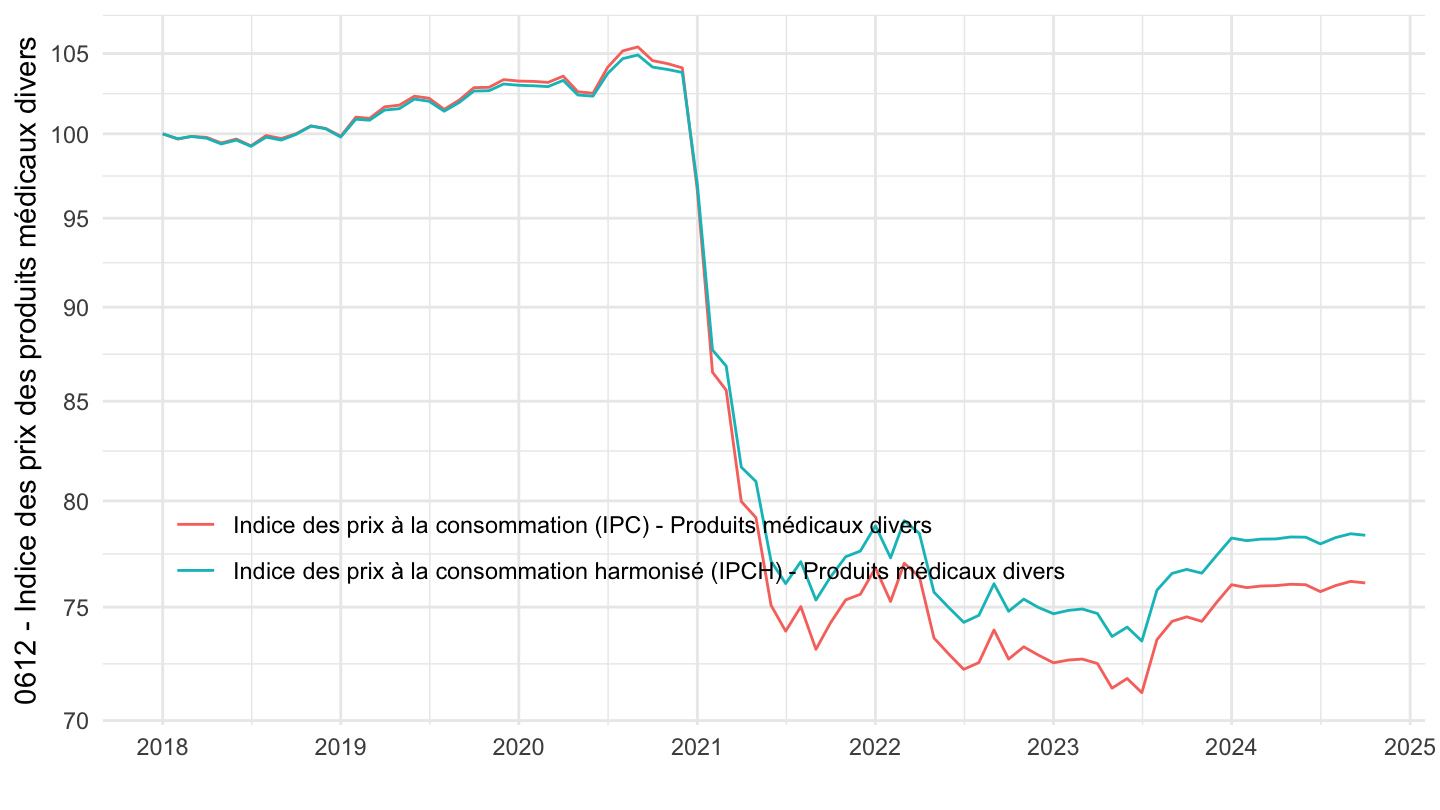
`IPCH-2015` |>
  bind_rows(`IPC-2015`) |>
  filter(COICOP2016 %in% c("0612"),
         NATURE == "INDICE",
         REF_AREA == "FE",
         FREQ == "M",
         is.na(MENAGES_IPC) | MENAGES_IPC == "ENSEMBLE") |>
  month_to_date() |>

  group_by(INDICATEUR) |>
  filter(date >= as.Date("2020-01-01")) |>
  arrange(date) |>
  mutate(OBS_VALUE = 100*OBS_VALUE/OBS_VALUE[date == as.Date("2020-01-01")]) |>
  ggplot() + ylab("0612 - Indice des prix des produits médicaux divers") + xlab("") + theme_minimal() +
  geom_line(aes(x = date, y = OBS_VALUE, color = paste0(Indicateur, " - Produits médicaux divers"))) +

  scale_x_date(breaks = seq.Date(as.Date("2019-12-01"), Sys.Date(), "3 months"),
               labels = date_format("%b %Y")) +
  theme(legend.position = c(0.4, 0.25),
        legend.title = element_blank()) +
  scale_y_log10(breaks = seq(10, 300, 5),
                     labels = dollar_format(accuracy = 1, prefix = ""))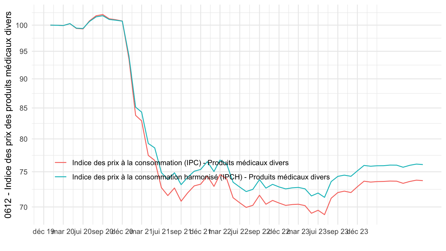
`IPCH-2015` |>
  bind_rows(`IPC-2015`) |>
  filter(COICOP2016 %in% c("0613"),
         NATURE == "INDICE",
         REF_AREA == "FE",
         FREQ == "M",
         is.na(MENAGES_IPC) | MENAGES_IPC == "ENSEMBLE") |>
  month_to_date() |>

  group_by(INDICATEUR) |>
  filter(date >= as.Date("1996-01-01")) |>
  arrange(date) |>
  mutate(OBS_VALUE = 100*OBS_VALUE/OBS_VALUE[date == as.Date("2000-01-01")]) |>
  ggplot() + ylab("Indice des prix des appareils et matériel thérapeutique") + xlab("") + theme_minimal() +
  geom_line(aes(x = date, y = OBS_VALUE, color = Indicateur)) +

  scale_x_date(breaks = seq(1920, 2100, 2) |> paste0("-01-01") |> as.Date(),
               labels = date_format("%Y")) +
  theme(legend.position = c(0.7, 0.2),
        legend.title = element_blank()) +
  scale_y_log10(breaks = seq(10, 300, 5),
                     labels = dollar_format(accuracy = 1, prefix = ""))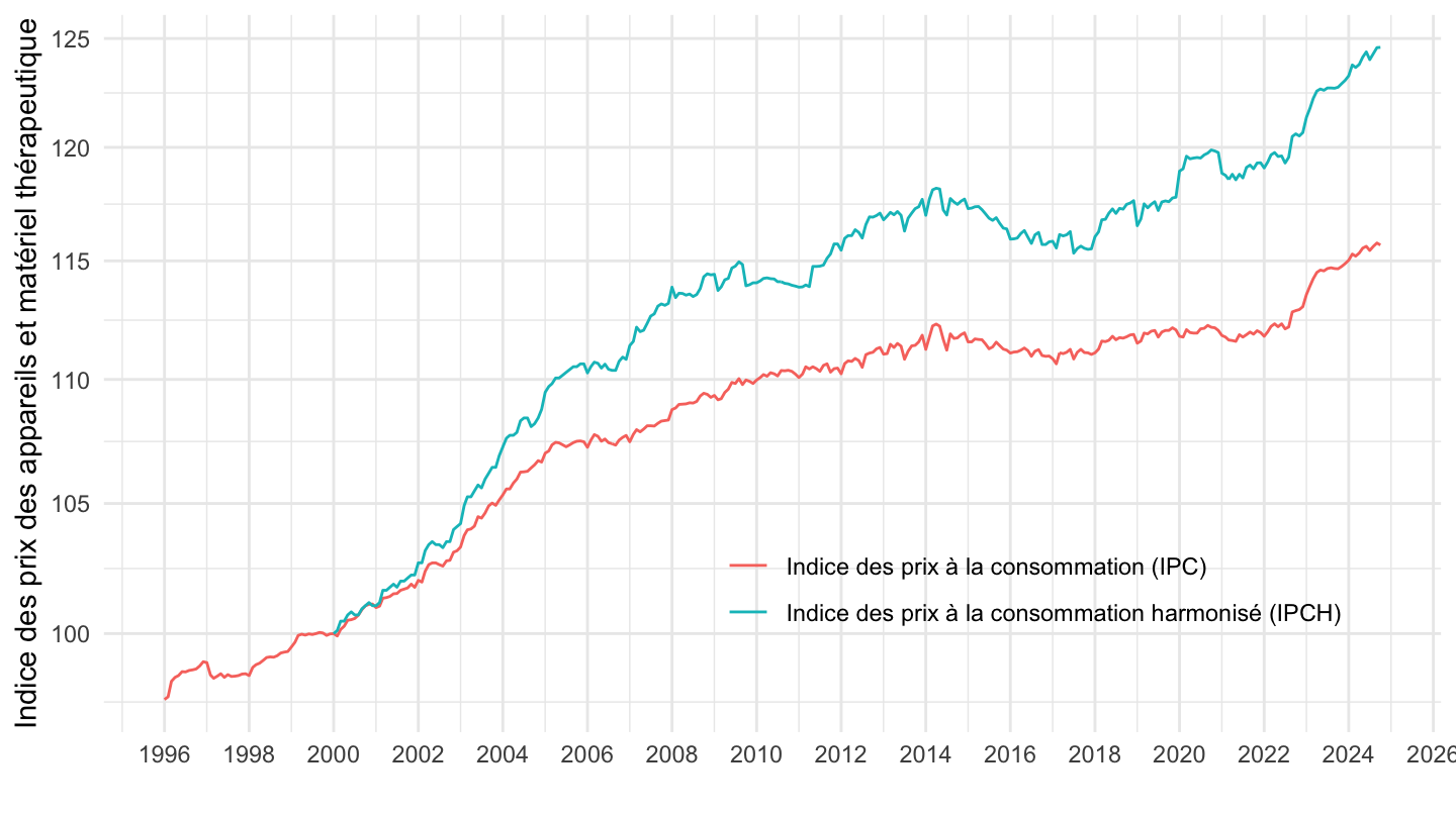
`IPCH-2015` |>
  bind_rows(`IPC-2015`) |>
  filter(COICOP2016 %in% c("0621"),
         NATURE == "INDICE",
         REF_AREA == "FE",
         FREQ == "M",
         is.na(MENAGES_IPC) | MENAGES_IPC == "ENSEMBLE") |>
  month_to_date() |>

  group_by(INDICATEUR) |>
  filter(date >= as.Date("1996-01-01")) |>
  arrange(date) |>
  mutate(OBS_VALUE = 100*OBS_VALUE/OBS_VALUE[date == as.Date("2000-01-01")]) |>
  ggplot() + ylab("Indice des prix des Services médicaux") + xlab("") + theme_minimal() +
  geom_line(aes(x = date, y = OBS_VALUE, color = Indicateur)) +

  scale_x_date(breaks = seq(1920, 2100, 2) |> paste0("-01-01") |> as.Date(),
               labels = date_format("%Y")) +
  theme(legend.position = c(0.7, 0.2),
        legend.title = element_blank()) +
  scale_y_log10(breaks = seq(10, 300, 5),
                     labels = dollar_format(accuracy = 1, prefix = ""))
`IPCH-2015` |>
  bind_rows(`IPC-2015`) |>
  filter(COICOP2016 %in% c("0622"),
         NATURE == "INDICE",
         REF_AREA == "FE",
         FREQ == "M",
         is.na(MENAGES_IPC) | MENAGES_IPC == "ENSEMBLE") |>
  month_to_date() |>

  group_by(INDICATEUR) |>
  filter(date >= as.Date("1996-01-01")) |>
  arrange(date) |>
  mutate(OBS_VALUE = 100*OBS_VALUE/OBS_VALUE[date == as.Date("2000-01-01")]) |>
  ggplot() + ylab("Indice des prix des Services médicaux") + xlab("") + theme_minimal() +
  geom_line(aes(x = date, y = OBS_VALUE, color = Indicateur)) +

  scale_x_date(breaks = seq(1920, 2100, 2) |> paste0("-01-01") |> as.Date(),
               labels = date_format("%Y")) +
  theme(legend.position = c(0.7, 0.2),
        legend.title = element_blank()) +
  scale_y_log10(breaks = seq(10, 300, 5),
                     labels = dollar_format(accuracy = 1, prefix = ""))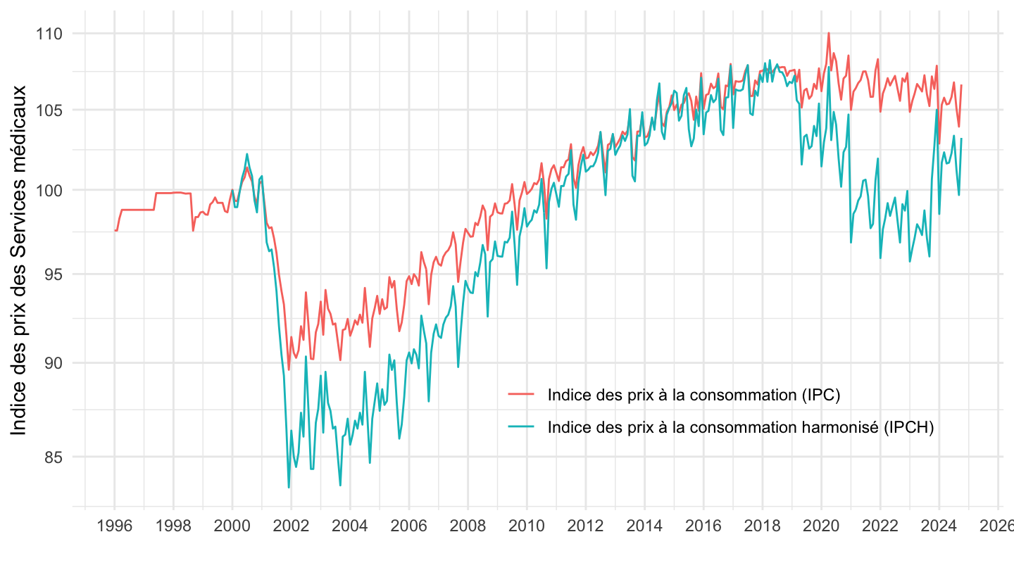
`IPCH-2015` |>
  bind_rows(`IPC-2015`) |>
  filter(COICOP2016 %in% c("0623"),
         NATURE == "INDICE",
         REF_AREA == "FE",
         FREQ == "M",
         is.na(MENAGES_IPC) | MENAGES_IPC == "ENSEMBLE") |>
  month_to_date() |>

  group_by(INDICATEUR) |>
  filter(date >= as.Date("1996-01-01")) |>
  arrange(date) |>
  mutate(OBS_VALUE = 100*OBS_VALUE/OBS_VALUE[date == as.Date("2000-01-01")]) |>
  ggplot() + ylab("Indice des prix des Services paramédicaux") + xlab("") + theme_minimal() +
  geom_line(aes(x = date, y = OBS_VALUE, color = Indicateur)) +

  scale_x_date(breaks = seq(1920, 2100, 2) |> paste0("-01-01") |> as.Date(),
               labels = date_format("%Y")) +
  theme(legend.position = c(0.7, 0.2),
        legend.title = element_blank()) +
  scale_y_log10(breaks = seq(10, 300, 5),
                     labels = dollar_format(accuracy = 1, prefix = ""))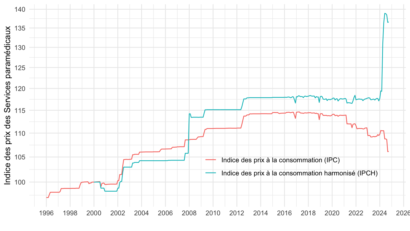
`IPCH-2015` |>
  bind_rows(`IPC-2015`) |>
  filter(COICOP2016 %in% c("10"),
         NATURE == "INDICE",
         REF_AREA == "FE",
         FREQ == "M",
         is.na(MENAGES_IPC) | MENAGES_IPC == "ENSEMBLE") |>
  month_to_date() |>

  group_by(INDICATEUR) |>
  filter(date >= as.Date("1996-01-01")) |>
  arrange(date) |>
  mutate(OBS_VALUE = 100*OBS_VALUE/OBS_VALUE[1]) |>
  ggplot() + ylab("Indice des prix, Enseignement") + xlab("") + theme_minimal() +
  geom_line(aes(x = date, y = OBS_VALUE, color = Indicateur)) +

  scale_x_date(breaks = seq(1920, 2100, 2) |> paste0("-01-01") |> as.Date(),
               labels = date_format("%Y")) +
  theme(legend.position = c(0.7, 0.2),
        legend.title = element_blank()) +
  scale_y_log10(breaks = seq(10, 300, 5),
                     labels = dollar_format(accuracy = 1, prefix = ""))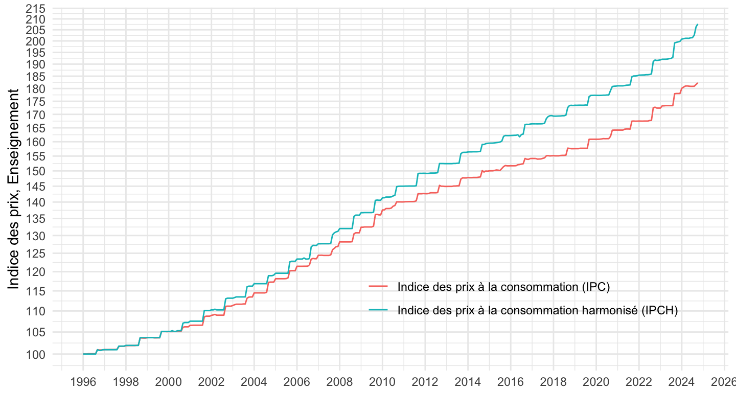
`IPCH-2015` |>
  bind_rows(`IPC-2015`) |>
  filter(COICOP2016 %in% c("10"),
         NATURE == "INDICE",
         REF_AREA == "FE",
         FREQ == "M",
         is.na(MENAGES_IPC) | MENAGES_IPC == "ENSEMBLE") |>
  month_to_date() |>

  group_by(INDICATEUR) |>
  filter(date >= as.Date("2002-01-01")) |>
  arrange(date) |>
  mutate(OBS_VALUE = 100*OBS_VALUE/OBS_VALUE[1]) |>
  ggplot() + ylab("Indice des prix, Enseignement") + xlab("") + theme_minimal() +
  geom_line(aes(x = date, y = OBS_VALUE, color = Indicateur)) +

  scale_x_date(breaks = seq(1920, 2100, 2) |> paste0("-01-01") |> as.Date(),
               labels = date_format("%Y")) +
  theme(legend.position = c(0.7, 0.2),
        legend.title = element_blank()) +
  scale_y_log10(breaks = seq(10, 300, 5),
                     labels = dollar_format(accuracy = 1, prefix = ""))
`IPCH-2015` |>
  bind_rows(`IPC-2015`) |>
  filter(COICOP2016 %in% c("101"),
         NATURE == "INDICE",
         REF_AREA == "FE",
         FREQ == "M",
         is.na(MENAGES_IPC) | MENAGES_IPC == "ENSEMBLE") |>
  month_to_date() |>

  group_by(INDICATEUR) |>
  filter(date >= as.Date("1996-01-01")) |>
  arrange(date) |>
  mutate(OBS_VALUE = 100*OBS_VALUE/OBS_VALUE[1]) |>
  ggplot() + ylab("Indice des prix, Enseignement") + xlab("") + theme_minimal() +
  geom_line(aes(x = date, y = OBS_VALUE, color = Indicateur)) +

  scale_x_date(breaks = seq(1920, 2100, 2) |> paste0("-01-01") |> as.Date(),
               labels = date_format("%Y")) +
  theme(legend.position = c(0.7, 0.2),
        legend.title = element_blank()) +
  scale_y_log10(breaks = seq(10, 300, 5),
                     labels = dollar_format(accuracy = 1, prefix = ""))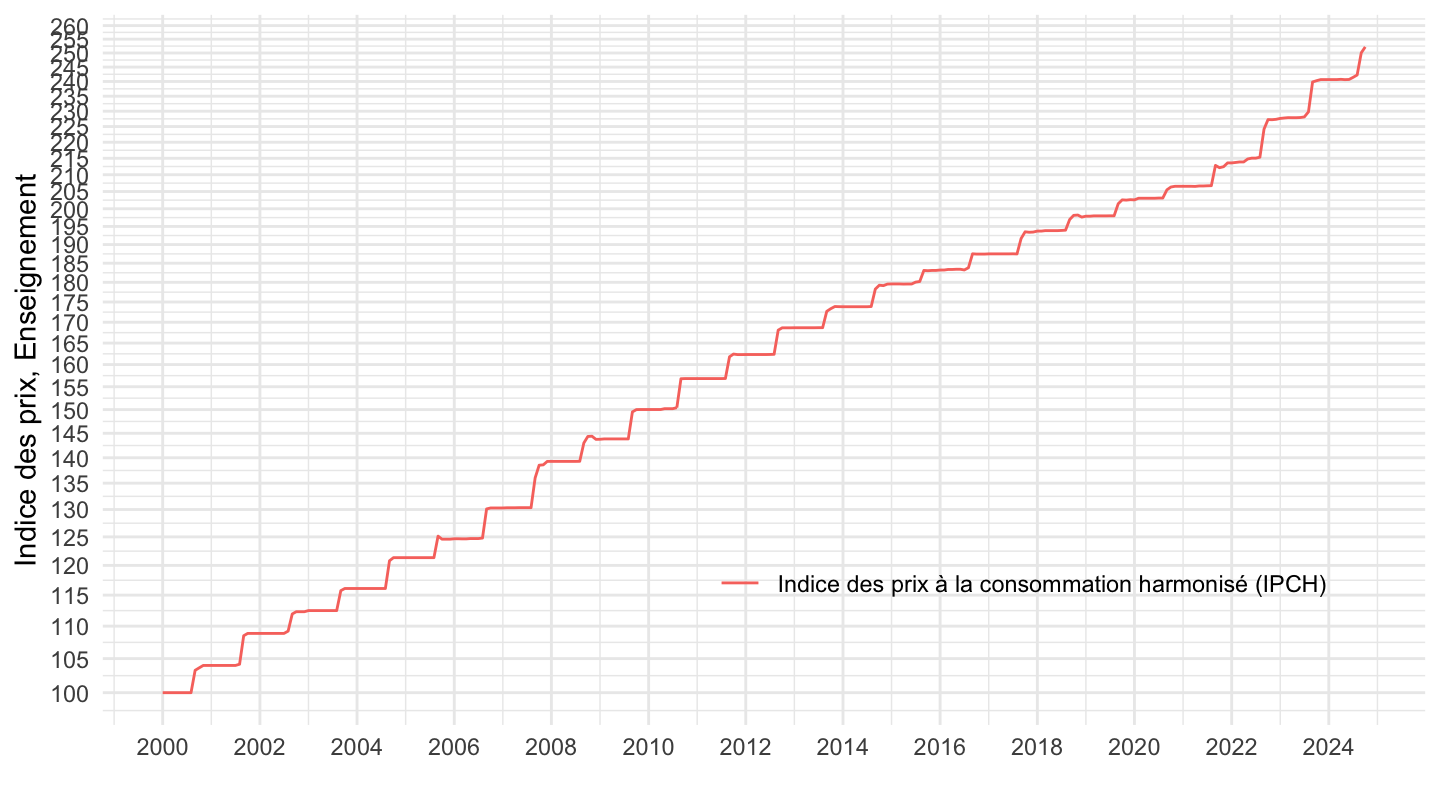
`IPCH-2015` |>
  bind_rows(`IPC-2015`) |>
  filter(COICOP2016 %in% c("102"),
         NATURE == "INDICE",
         REF_AREA == "FE",
         FREQ == "M",
         is.na(MENAGES_IPC) | MENAGES_IPC == "ENSEMBLE") |>
  month_to_date() |>

  group_by(INDICATEUR) |>
  filter(date >= as.Date("1996-01-01")) |>
  arrange(date) |>
  mutate(OBS_VALUE = 100*OBS_VALUE/OBS_VALUE[1]) |>
  ggplot() + ylab("Indice des prix, Enseignement") + xlab("") + theme_minimal() +
  geom_line(aes(x = date, y = OBS_VALUE, color = Indicateur)) +

  scale_x_date(breaks = seq(1920, 2100, 2) |> paste0("-01-01") |> as.Date(),
               labels = date_format("%Y")) +
  theme(legend.position = c(0.7, 0.2),
        legend.title = element_blank()) +
  scale_y_log10(breaks = seq(10, 300, 5),
                     labels = dollar_format(accuracy = 1, prefix = ""))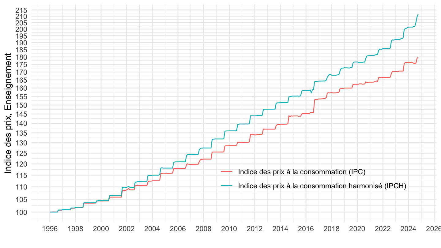
`IPCH-2015` |>
  bind_rows(`IPC-2015`) |>
  filter(COICOP2016 %in% c("104"),
         NATURE == "INDICE",
         REF_AREA == "FE",
         FREQ == "M",
         is.na(MENAGES_IPC) | MENAGES_IPC == "ENSEMBLE") |>
  month_to_date() |>

  group_by(INDICATEUR) |>
  filter(date >= as.Date("1996-01-01")) |>
  arrange(date) |>
  mutate(OBS_VALUE = 100*OBS_VALUE/OBS_VALUE[1]) |>
  ggplot() + ylab("Indice des prix, Enseignement") + xlab("") + theme_minimal() +
  geom_line(aes(x = date, y = OBS_VALUE, color = Indicateur)) +

  scale_x_date(breaks = seq(1920, 2100, 2) |> paste0("-01-01") |> as.Date(),
               labels = date_format("%Y")) +
  theme(legend.position = c(0.7, 0.2),
        legend.title = element_blank()) +
  scale_y_log10(breaks = seq(10, 300, 5),
                     labels = dollar_format(accuracy = 1, prefix = ""))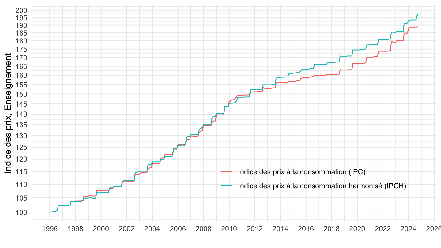
`IPCH-2015` |>
  bind_rows(`IPC-2015`) |>
  filter(COICOP2016 %in% c("09"),
         NATURE == "INDICE",
         REF_AREA == "FE",
         FREQ == "M",
         is.na(MENAGES_IPC) | MENAGES_IPC == "ENSEMBLE") |>
  month_to_date() |>

  group_by(INDICATEUR) |>
  filter(date >= as.Date("1996-01-01")) |>
  arrange(date) |>
  mutate(OBS_VALUE = 100*OBS_VALUE/OBS_VALUE[date == as.Date("1996-01-01")]) |>
  ggplot() + ylab("Indice des prix, Loisirs et Culture") + xlab("") + theme_minimal() +
  geom_line(aes(x = date, y = OBS_VALUE, color = Indicateur)) +

  scale_x_date(breaks = seq(1920, 2100, 2) |> paste0("-01-01") |> as.Date(),
               labels = date_format("%Y")) +
  theme(legend.position = c(0.7, 0.2),
        legend.title = element_blank()) +
  scale_y_log10(breaks = seq(10, 300, 5),
                     labels = dollar_format(accuracy = 1, prefix = ""))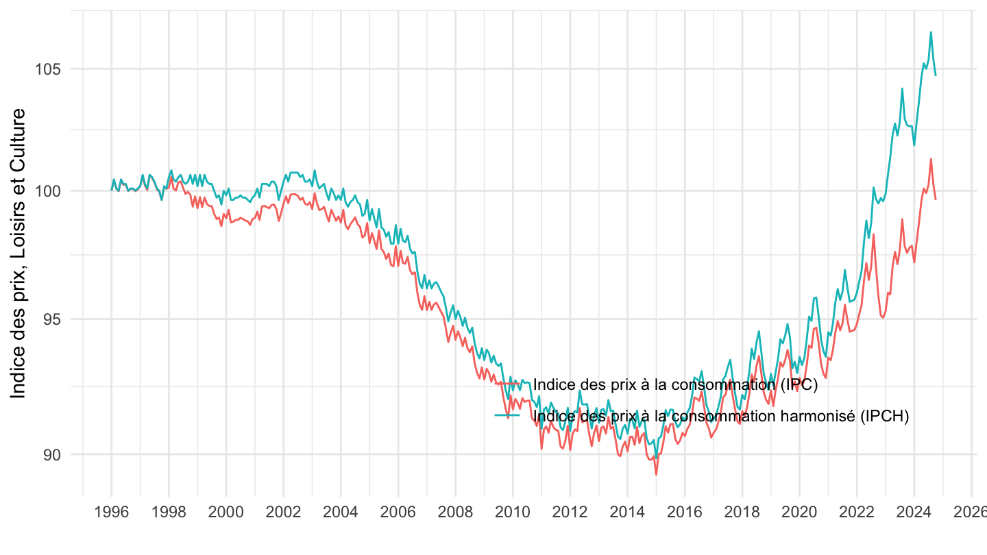
Jeux d’argent et de hasard: 13,4 milliards d’euros. Dépense de consommation finale des ménages s’établit à 1 262,5 Md€ toutes taxes comprises pour l’année 2019, soit 51,9 % du produit intérieur brut (PIB).
`IPCH-2015` |>
  bind_rows(`IPC-2015`) |>
  filter(COICOP2016 %in% c("09430"),
         NATURE == "INDICE",
         REF_AREA == "FE",
         FREQ == "M",
         is.na(MENAGES_IPC) | MENAGES_IPC == "ENSEMBLE") |>
  month_to_date() |>

  group_by(INDICATEUR) |>
  filter(date >= as.Date("1996-01-01")) |>
  arrange(desc(date)) |>
  mutate(OBS_VALUE = 100*OBS_VALUE/OBS_VALUE[1]) |>
  ggplot() + ylab("Indice des prix, Tickets à gratter") + xlab("") + theme_minimal() +
  geom_line(aes(x = date, y = OBS_VALUE, color = Indicateur)) +
  scale_x_date(breaks = seq(1920, 2100, 1) |> paste0("-01-01") |> as.Date(),
               labels = date_format("%Y")) +
  theme(legend.position = c(0.3, 0.3),
        legend.title = element_blank()) +
  scale_y_log10(breaks = seq(10, 300, 1),
                     labels = dollar_format(accuracy = 1, prefix = ""))
`IPCH-2015` |>
  bind_rows(`IPC-2015`) |>
  filter(COICOP2016 %in% c("09430"),
         NATURE == "INDICE",
         REF_AREA == "FE",
         FREQ == "M",
         is.na(MENAGES_IPC) | MENAGES_IPC == "ENSEMBLE") |>
  month_to_date() |>

  group_by(INDICATEUR) |>
  filter(date >= as.Date("1996-01-01"),
         date <= as.Date("2024-05-01")) |>
  arrange(desc(date)) |>
  mutate(OBS_VALUE = 100*OBS_VALUE/OBS_VALUE[1]) |>
  ggplot() + ylab("Indice des prix, Tickets à gratter") + xlab("") + theme_minimal() +
  geom_line(aes(x = date, y = OBS_VALUE, color = Indicateur)) +
  scale_x_date(breaks = seq(1920, 2100, 1) |> paste0("-01-01") |> as.Date(),
               labels = date_format("%Y")) +
  theme(legend.position = c(0.3, 0.3),
        legend.title = element_blank()) +
  scale_y_log10(breaks = seq(10, 300, 1),
                     labels = dollar_format(accuracy = 1, prefix = ""))
`IPCH-2015` |>
  bind_rows(`IPC-2015`) |>
  filter(COICOP2016 %in% c("09423"),
         NATURE == "INDICE",
         REF_AREA == "FE",
         FREQ == "M",
         is.na(MENAGES_IPC) | MENAGES_IPC == "ENSEMBLE") |>
  month_to_date() |>

  group_by(INDICATEUR) |>
  filter(date >= as.Date("1996-01-01")) |>
  arrange(date) |>
  mutate(OBS_VALUE = 100*OBS_VALUE/OBS_VALUE[date == as.Date("1996-01-01")]) |>
  ggplot() + ylab("Indice des prix, redevances (Redevance audiviosuelle)") + xlab("") + theme_minimal() +
  geom_line(aes(x = date, y = OBS_VALUE, color = Indicateur)) +
  scale_x_date(breaks = seq(1920, 2100, 2) |> paste0("-01-01") |> as.Date(),
               labels = date_format("%Y")) +
  theme(legend.position = c(0.3, 0.8),
        legend.title = element_blank()) +
  scale_y_log10(breaks = seq(10, 300, 5),
                     labels = dollar_format(accuracy = 1, prefix = ""))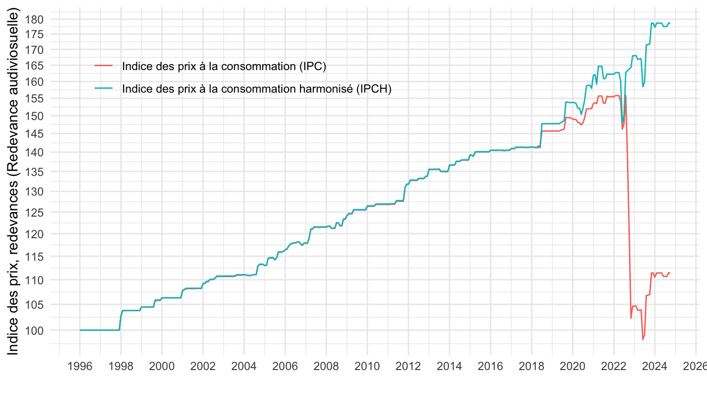
`IPCH-2015` |>
  bind_rows(`IPC-2015`) |>
  filter(COICOP2016 %in% c("09423"),
         NATURE == "INDICE",
         REF_AREA == "FE",
         FREQ == "M",
         is.na(MENAGES_IPC) | MENAGES_IPC == "ENSEMBLE") |>
  month_to_date() |>

  group_by(INDICATEUR) |>
  filter(date >= as.Date("2015-01-01")) |>
  arrange(date) |>
  mutate(OBS_VALUE = 100*OBS_VALUE/OBS_VALUE[date == as.Date("2015-01-01")]) |>
  ggplot() + ylab("Indice des prix, redevances (Redevance audiviosuelle)") + xlab("") + theme_minimal() +
  geom_line(aes(x = date, y = OBS_VALUE, color = Indicateur)) +
  scale_x_date(breaks = seq(1920, 2100, 1) |> paste0("-01-01") |> as.Date(),
               labels = date_format("%Y")) +
  theme(legend.position = c(0.3, 0.8),
        legend.title = element_blank()) +
  scale_y_log10(breaks = seq(10, 300, 5),
                     labels = dollar_format(accuracy = 1, prefix = ""))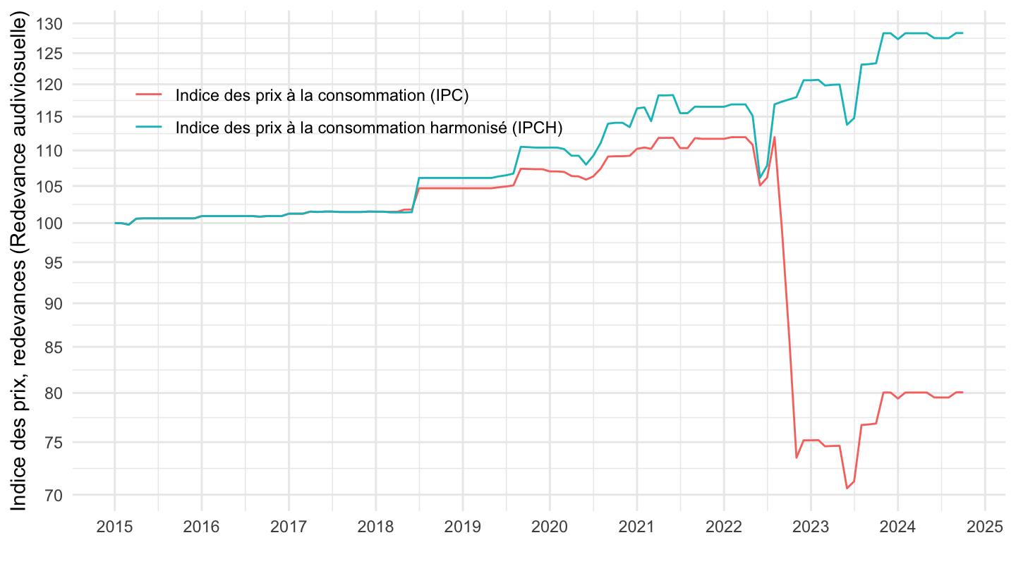
`IPCH-2015` |>
  bind_rows(`IPC-2015`) |>
  filter(COICOP2016 %in% c("05"),
         NATURE == "INDICE",
         REF_AREA == "FE",
         FREQ == "M",
         is.na(MENAGES_IPC) | MENAGES_IPC == "ENSEMBLE") |>
  month_to_date() |>

  group_by(INDICATEUR) |>
  filter(date >= as.Date("1996-01-01")) |>
  arrange(date) |>
  mutate(OBS_VALUE = 100*OBS_VALUE/OBS_VALUE[date == as.Date("1996-01-01")]) |>
  ggplot() + ylab("05 - Meubles, articles de ménage et entretien courant du foyer") + xlab("") + theme_minimal() +
  geom_line(aes(x = date, y = OBS_VALUE, color = Indicateur)) +

  scale_x_date(breaks = seq(1920, 2100, 2) |> paste0("-01-01") |> as.Date(),
               labels = date_format("%Y")) +
  theme(legend.position = c(0.3, 0.8),
        legend.title = element_blank()) +
  scale_y_log10(breaks = seq(10, 300, 5),
                     labels = dollar_format(accuracy = 1, prefix = ""))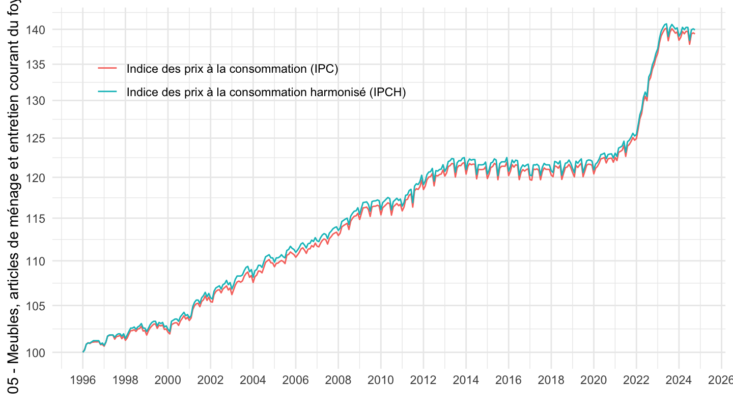
`IPCH-2015` |>
  bind_rows(`IPC-2015`) |>
  filter(COICOP2016 %in% c("0562"),
         NATURE == "INDICE",
         REF_AREA == "FE",
         FREQ == "M",
         is.na(MENAGES_IPC) | MENAGES_IPC == "ENSEMBLE") |>
  month_to_date() |>

  group_by(INDICATEUR) |>
  filter(date >= as.Date("1996-01-01")) |>
  arrange(date) |>
  mutate(OBS_VALUE = 100*OBS_VALUE/OBS_VALUE[date == as.Date("1998-01-01")]) |>
  ggplot() + ylab("05.6.2 - Services domestiques et services ménagers") + xlab("") + theme_minimal() +
  geom_line(aes(x = date, y = OBS_VALUE, color = Indicateur)) +

  scale_x_date(breaks = seq(1920, 2100, 2) |> paste0("-01-01") |> as.Date(),
               labels = date_format("%Y")) +
  theme(legend.position = c(0.3, 0.8),
        legend.title = element_blank()) +
  scale_y_log10(breaks = seq(10, 300, 5),
                     labels = dollar_format(accuracy = 1, prefix = ""))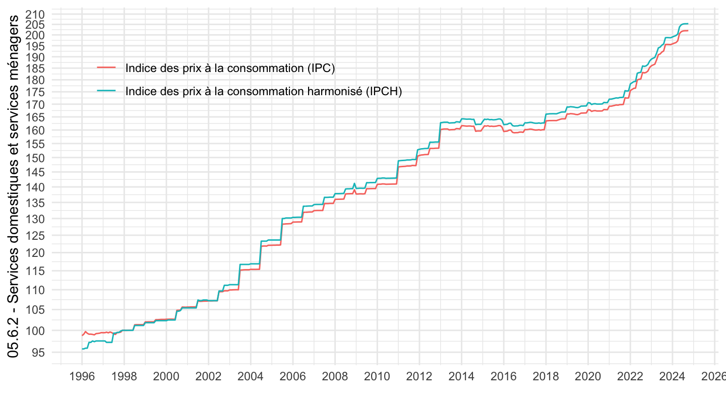
`IPCH-2015` |>
  bind_rows(`IPC-2015`) |>
  filter(COICOP2016 %in% c("05621"),
         NATURE == "INDICE",
         REF_AREA == "FE",
         FREQ == "M",
         is.na(MENAGES_IPC) | MENAGES_IPC == "ENSEMBLE") |>
  month_to_date() |>

  group_by(INDICATEUR) |>
  filter(date >= as.Date("1996-01-01")) |>
  arrange(date) |>
  mutate(OBS_VALUE = 100*OBS_VALUE/OBS_VALUE[date == as.Date("1998-01-01")]) |>
  ggplot() + ylab("05621") + xlab("") + theme_minimal() +
  geom_line(aes(x = date, y = OBS_VALUE, color = Indicateur)) +

  scale_x_date(breaks = seq(1920, 2100, 2) |> paste0("-01-01") |> as.Date(),
               labels = date_format("%Y")) +
  theme(legend.position = c(0.3, 0.2),
        legend.title = element_blank()) +
  scale_y_log10(breaks = seq(10, 300, 5),
                     labels = dollar_format(accuracy = 1, prefix = ""))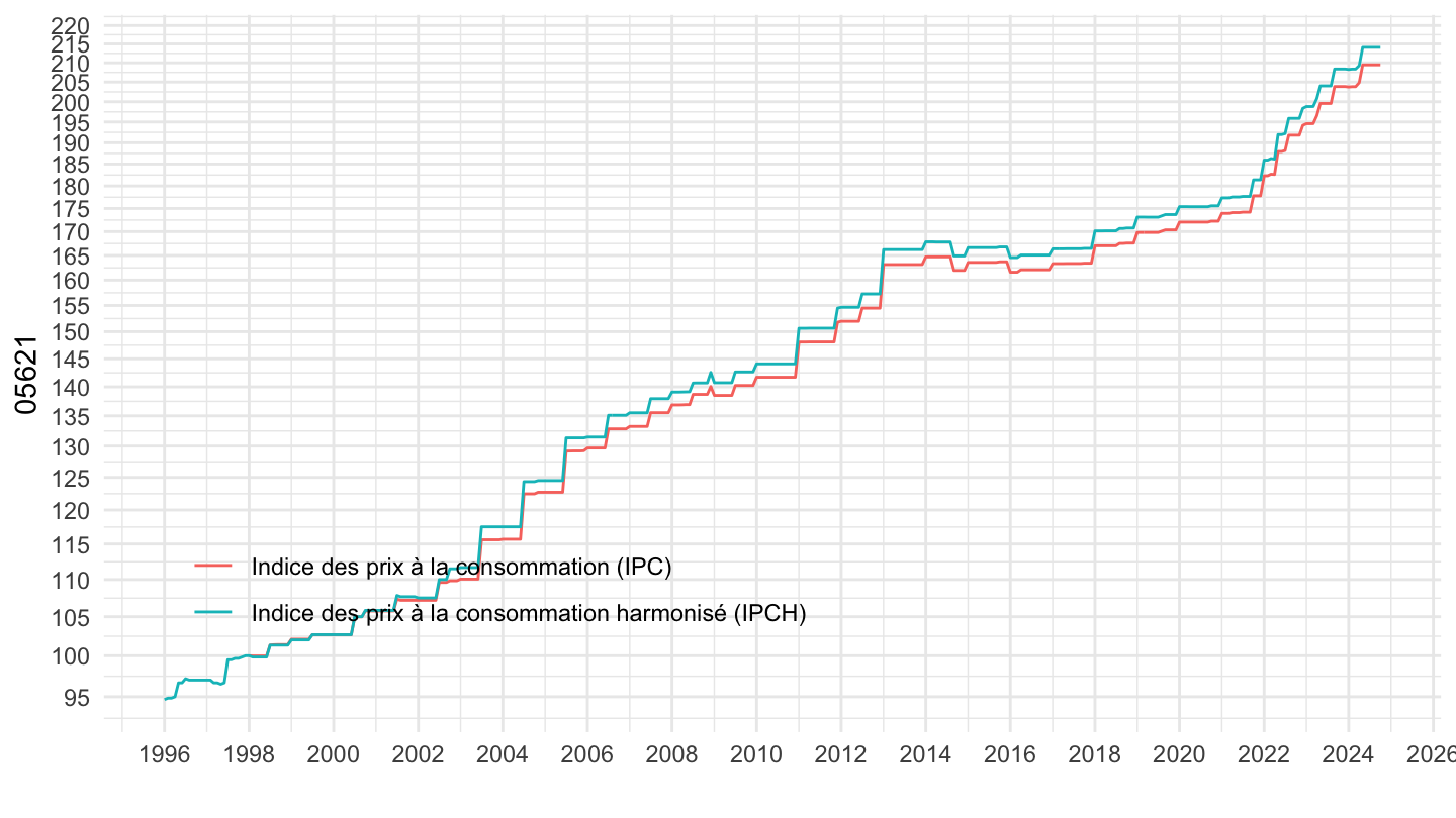
`IPCH-2015` |>
  bind_rows(`IPC-2015`) |>
  filter(COICOP2016 %in% c("01"),
         NATURE == "INDICE",
         REF_AREA == "FE",
         FREQ == "M",
         is.na(MENAGES_IPC) | MENAGES_IPC == "ENSEMBLE") |>
  month_to_date() |>

  group_by(INDICATEUR) |>
  filter(date >= as.Date("1996-01-01")) |>
  arrange(date) |>
  mutate(OBS_VALUE = 100*OBS_VALUE/OBS_VALUE[date == as.Date("1996-01-01")]) |>
  ggplot() + ylab("Indice des prix, Ensemble") + xlab("") + theme_minimal() +
  geom_line(aes(x = date, y = OBS_VALUE, color = Indicateur)) +

  scale_x_date(breaks = seq(1920, 2100, 2) |> paste0("-01-01") |> as.Date(),
               labels = date_format("%Y")) +
  theme(legend.position = c(0.7, 0.2),
        legend.title = element_blank()) +
  scale_y_log10(breaks = seq(10, 300, 5),
                     labels = dollar_format(accuracy = 1, prefix = ""))
`IPCH-2015` |>
  bind_rows(`IPC-2015`) |>
  filter(COICOP2016 %in% c("01"),
         NATURE == "INDICE",
         REF_AREA == "FE",
         FREQ == "M",
         is.na(MENAGES_IPC) | MENAGES_IPC == "ENSEMBLE") |>
  month_to_date() |>

  group_by(INDICATEUR) |>
  filter(date >= as.Date("1996-01-01")) |>
  arrange(date) |>
  mutate(OBS_VALUE = OBS_VALUE/lag(OBS_VALUE, 12)-1) |>
  ggplot() + ylab("Indice des prix, Ensemble") + xlab("") + theme_minimal() +
  geom_line(aes(x = date, y = OBS_VALUE, color = Indicateur)) +

  scale_x_date(breaks = seq(1920, 2100, 2) |> paste0("-01-01") |> as.Date(),
               labels = date_format("%Y")) +
  theme(legend.position = c(0.3, 0.8),
        legend.title = element_blank()) +
  scale_y_continuous(breaks = 0.01*seq(-10, 40, 2),
                     labels = percent_format(accuracy = 1, prefix = ""))
`IPCH-2015` |>
  bind_rows(`IPC-2015`) |>
  filter(COICOP2016 %in% c("02"),
         NATURE == "INDICE",
         REF_AREA == "FE",
         FREQ == "M",
         is.na(MENAGES_IPC) | MENAGES_IPC == "ENSEMBLE") |>
  month_to_date() |>

  group_by(INDICATEUR) |>
  filter(date >= as.Date("1996-01-01")) |>
  arrange(date) |>
  mutate(OBS_VALUE = 100*OBS_VALUE/OBS_VALUE[date == as.Date("1996-01-01")]) |>
  ggplot() + ylab("Indice des prix, Boissons") + xlab("") + theme_minimal() +
  geom_line(aes(x = date, y = OBS_VALUE, color = Indicateur)) +

  scale_x_date(breaks = seq(1920, 2100, 2) |> paste0("-01-01") |> as.Date(),
               labels = date_format("%Y")) +
  theme(legend.position = c(0.7, 0.2),
        legend.title = element_blank()) +
  scale_y_log10(breaks = seq(10, 300, 5),
                     labels = dollar_format(accuracy = 1, prefix = ""))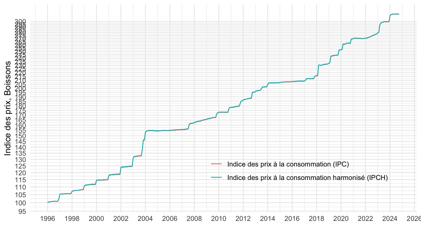
`IPCH-2015` |>
  bind_rows(`IPC-2015`) |>
  filter(COICOP2016 %in% c("02"),
         NATURE == "INDICE",
         REF_AREA == "FE",
         FREQ == "M",
         is.na(MENAGES_IPC) | MENAGES_IPC == "ENSEMBLE") |>
  month_to_date() |>

  group_by(INDICATEUR) |>
  filter(date >= as.Date("1996-01-01")) |>
  arrange(date) |>
  mutate(OBS_VALUE = OBS_VALUE/lag(OBS_VALUE, 12)-1) |>
  ggplot() + ylab("Indice des prix, Ensemble") + xlab("") + theme_minimal() +
  geom_line(aes(x = date, y = OBS_VALUE, color = Indicateur)) +

  scale_x_date(breaks = seq(1920, 2100, 2) |> paste0("-01-01") |> as.Date(),
               labels = date_format("%Y")) +
  theme(legend.position = c(0.3, 0.8),
        legend.title = element_blank()) +
  scale_y_continuous(breaks = 0.01*seq(-10, 40, 2),
                     labels = percent_format(accuracy = 1, prefix = ""))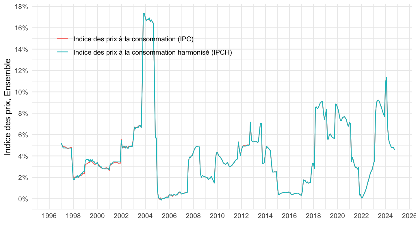
`IPCH-2015` |>
  bind_rows(`IPC-2015`) |>
  filter(COICOP2016 %in% c("11"),
         NATURE == "INDICE",
         REF_AREA == "FE",
         FREQ == "M",
         is.na(MENAGES_IPC) | MENAGES_IPC == "ENSEMBLE") |>
  month_to_date() |>

  group_by(INDICATEUR) |>
  filter(date >= as.Date("1996-01-01")) |>
  arrange(date) |>
  mutate(OBS_VALUE = 100*OBS_VALUE/OBS_VALUE[date == as.Date("1996-01-01")]) |>
  ggplot() + ylab("Indice des prix, Restaurants") + xlab("") + theme_minimal() +
  geom_line(aes(x = date, y = OBS_VALUE, color = Indicateur)) +

  scale_x_date(breaks = seq(1920, 2100, 2) |> paste0("-01-01") |> as.Date(),
               labels = date_format("%Y")) +
  theme(legend.position = c(0.7, 0.2),
        legend.title = element_blank()) +
  scale_y_log10(breaks = seq(10, 300, 5),
                     labels = dollar_format(accuracy = 1, prefix = ""))
`IPCH-2015` |>
  bind_rows(`IPC-2015`) |>
  filter(COICOP2016 %in% c("1112"),
         NATURE == "INDICE",
         REF_AREA == "FE",
         FREQ == "M",
         is.na(MENAGES_IPC) | MENAGES_IPC == "ENSEMBLE") |>
  month_to_date() |>

  group_by(INDICATEUR) |>
  filter(date >= as.Date("1996-01-01")) |>
  arrange(date) |>
  mutate(OBS_VALUE = 100*OBS_VALUE/OBS_VALUE[date == as.Date("1998-01-01")]) |>
  ggplot() + ylab("Cantines") + xlab("") + theme_minimal() +
  geom_line(aes(x = date, y = OBS_VALUE, color = Indicateur)) +

  scale_x_date(breaks = seq(1920, 2100, 2) |> paste0("-01-01") |> as.Date(),
               labels = date_format("%Y")) +
  theme(legend.position = c(0.3, 0.8),
        legend.title = element_blank()) +
  scale_y_log10(breaks = seq(10, 300, 5),
                     labels = dollar_format(accuracy = 1, prefix = ""))
`IPCH-2015` |>
  bind_rows(`IPC-2015`) |>
  filter(COICOP2016 %in% c("03"),
         NATURE == "INDICE",
         REF_AREA == "FE",
         FREQ == "M",
         is.na(MENAGES_IPC) | MENAGES_IPC == "ENSEMBLE") |>
  month_to_date() |>

  group_by(INDICATEUR) |>
  filter(date >= as.Date("1996-01-01")) |>
  arrange(date) |>
  mutate(OBS_VALUE = 100*OBS_VALUE/OBS_VALUE[date == as.Date("1996-01-01")]) |>
  ggplot() + ylab("Indice des prix, Habillement") + xlab("") + theme_minimal() +
  geom_line(aes(x = date, y = OBS_VALUE, color = Indicateur)) +

  scale_x_date(breaks = seq(1920, 2100, 2) |> paste0("-01-01") |> as.Date(),
               labels = date_format("%Y")) +
  theme(legend.position = c(0.7, 0.2),
        legend.title = element_blank()) +
  scale_y_log10(breaks = seq(10, 300, 5),
                     labels = dollar_format(accuracy = 1, prefix = ""))
`IPCH-2015` |>
  bind_rows(`IPC-2015`) |>
  filter(COICOP2016 %in% c("04"),
         NATURE == "INDICE",
         REF_AREA == "FE",
         FREQ == "M",
         is.na(MENAGES_IPC) | MENAGES_IPC == "ENSEMBLE") |>
  month_to_date() |>

  group_by(INDICATEUR) |>
  filter(date >= as.Date("1996-01-01")) |>
  arrange(date) |>
  mutate(OBS_VALUE = 100*OBS_VALUE/OBS_VALUE[date == as.Date("1996-01-01")]) |>
  ggplot() + ylab("Indice des prix, Logement") + xlab("") + theme_minimal() +
  geom_line(aes(x = date, y = OBS_VALUE, color = Indicateur)) +

  scale_x_date(breaks = seq(1920, 2100, 2) |> paste0("-01-01") |> as.Date(),
               labels = date_format("%Y")) +
  theme(legend.position = c(0.7, 0.2),
        legend.title = element_blank()) +
  scale_y_log10(breaks = seq(10, 300, 5),
                     labels = dollar_format(accuracy = 1, prefix = ""))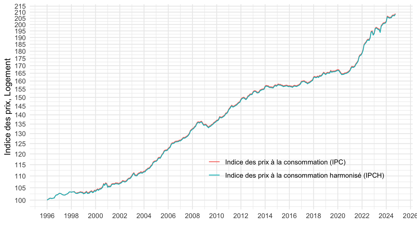
`IPCH-2015` |>
  bind_rows(`IPC-2015`) |>
  filter(COICOP2016 %in% c("041"),
         NATURE == "INDICE",
         REF_AREA == "FE",
         FREQ == "M",
         is.na(MENAGES_IPC) | MENAGES_IPC == "ENSEMBLE") |>
  month_to_date() |>

  group_by(INDICATEUR) |>
  filter(date >= as.Date("1996-01-01")) |>
  arrange(date) |>
  mutate(OBS_VALUE = 100*OBS_VALUE/OBS_VALUE[date == as.Date("1996-01-01")]) |>
  ggplot() + ylab("Indice des prix, Logement") + xlab("") + theme_minimal() +
  geom_line(aes(x = date, y = OBS_VALUE, color = Indicateur)) +

  scale_x_date(breaks = seq(1920, 2100, 2) |> paste0("-01-01") |> as.Date(),
               labels = date_format("%Y")) +
  theme(legend.position = c(0.7, 0.2),
        legend.title = element_blank()) +
  scale_y_log10(breaks = seq(10, 300, 5),
                     labels = dollar_format(accuracy = 1, prefix = ""))
`IPCH-2015` |>
  bind_rows(`IPC-2015`) |>
  filter(COICOP2016 %in% c("07"),
         NATURE == "INDICE",
         REF_AREA == "FE",
         FREQ == "M",
         is.na(MENAGES_IPC) | MENAGES_IPC == "ENSEMBLE") |>
  month_to_date() |>

  group_by(INDICATEUR) |>
  filter(date >= as.Date("1996-01-01")) |>
  arrange(date) |>
  mutate(OBS_VALUE = 100*OBS_VALUE/OBS_VALUE[date == as.Date("1996-01-01")]) |>
  ggplot() + ylab("Indice des prix, Transports") + xlab("") + theme_minimal() +
  geom_line(aes(x = date, y = OBS_VALUE, color = Indicateur)) +

  scale_x_date(breaks = seq(1920, 2100, 2) |> paste0("-01-01") |> as.Date(),
               labels = date_format("%Y")) +
  theme(legend.position = c(0.7, 0.2),
        legend.title = element_blank()) +
  scale_y_log10(breaks = seq(10, 300, 5),
                     labels = dollar_format(accuracy = 1, prefix = ""))
`IPCH-2015` |>
  bind_rows(`IPC-2015`) |>
  filter(COICOP2016 %in% c("07311"),
         NATURE == "INDICE",
         REF_AREA == "FE",
         FREQ == "M",
         is.na(MENAGES_IPC) | MENAGES_IPC == "ENSEMBLE") |>
  month_to_date() |>

  group_by(INDICATEUR) |>
  filter(date >= as.Date("1996-01-01")) |>
  arrange(date) |>
  mutate(OBS_VALUE = 100*OBS_VALUE/OBS_VALUE[date == as.Date("1996-01-01")]) |>
  ggplot() + ylab("Indice des prix, Transport de passagers par train") + xlab("") + theme_minimal() +
  geom_line(aes(x = date, y = OBS_VALUE, color = Indicateur)) +

  scale_x_date(breaks = seq(1920, 2100, 2) |> paste0("-01-01") |> as.Date(),
               labels = date_format("%Y")) +
  theme(legend.position = c(0.7, 0.2),
        legend.title = element_blank()) +
  scale_y_log10(breaks = seq(10, 300, 5),
                     labels = dollar_format(accuracy = 1, prefix = ""))
`IPCH-2015` |>
  bind_rows(`IPC-2015`) |>
  filter(COICOP2016 %in% c("08"),
         NATURE == "INDICE",
         REF_AREA == "FE",
         FREQ == "M",
         is.na(MENAGES_IPC) | MENAGES_IPC == "ENSEMBLE") |>
  month_to_date() |>

  group_by(INDICATEUR) |>
  filter(date >= as.Date("1996-01-01")) |>
  arrange(date) |>
  mutate(OBS_VALUE = 100*OBS_VALUE/OBS_VALUE[date == as.Date("1996-01-01")]) |>
  ggplot() + ylab("Indice des prix, Communications") + xlab("") + theme_minimal() +
  geom_line(aes(x = date, y = OBS_VALUE, color = Indicateur)) +

  scale_x_date(breaks = seq(1920, 2100, 2) |> paste0("-01-01") |> as.Date(),
               labels = date_format("%Y")) +
  theme(legend.position = c(0.3, 0.2),
        legend.title = element_blank()) +
  scale_y_log10(breaks = seq(10, 300, 5),
                     labels = dollar_format(accuracy = 1, prefix = ""))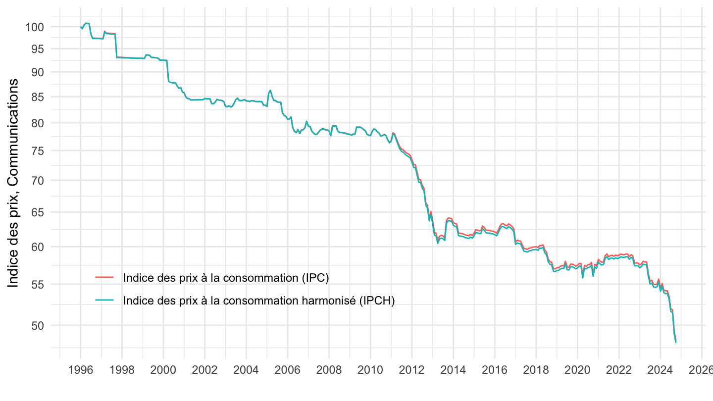
`IPCH-2015` |>
  bind_rows(`IPC-2015`) |>
  filter(COICOP2016 %in% c("12"),
         NATURE == "INDICE",
         REF_AREA == "FE",
         FREQ == "M",
         is.na(MENAGES_IPC) | MENAGES_IPC == "ENSEMBLE") |>
  month_to_date() |>

  group_by(INDICATEUR) |>
  filter(date >= as.Date("1996-01-01")) |>
  arrange(date) |>
  mutate(OBS_VALUE = 100*OBS_VALUE/OBS_VALUE[date == as.Date("1996-01-01")]) |>
  ggplot() + ylab("") + xlab("") + theme_minimal() +
  geom_line(aes(x = date, y = OBS_VALUE, color = Indicateur)) +

  scale_x_date(breaks = seq(1920, 2100, 2) |> paste0("-01-01") |> as.Date(),
               labels = date_format("%Y")) +
  theme(legend.position = c(0.3, 0.2),
        legend.title = element_blank()) +
  scale_y_log10(breaks = seq(10, 300, 5),
                     labels = dollar_format(accuracy = 1, prefix = ""))
`IPCH-2015` |>
  bind_rows(`IPC-2015`) |>
  filter(COICOP2016 %in% c("124"),
         NATURE == "INDICE",
         REF_AREA == "FE",
         FREQ == "M",
         is.na(MENAGES_IPC) | MENAGES_IPC == "ENSEMBLE") |>
  month_to_date() |>

  group_by(INDICATEUR) |>
  filter(date >= as.Date("1996-01-01")) |>
  arrange(date) |>
  mutate(OBS_VALUE = 100*OBS_VALUE/OBS_VALUE[1]) |>
  ggplot() + ylab("") + xlab("") + theme_minimal() +
  geom_line(aes(x = date, y = OBS_VALUE, color = Indicateur)) +

  scale_x_date(breaks = seq(1920, 2100, 2) |> paste0("-01-01") |> as.Date(),
               labels = date_format("%Y")) +
  theme(legend.position = c(0.3, 0.8),
        legend.title = element_blank()) +
  scale_y_log10(breaks = seq(10, 300, 5),
                     labels = dollar_format(accuracy = 1, prefix = ""))
`IPCH-2015` |>
  bind_rows(`IPC-2015`) |>
  filter(COICOP2016 %in% c("12401"),
         NATURE == "INDICE",
         REF_AREA == "FE",
         FREQ == "M",
         is.na(MENAGES_IPC) | MENAGES_IPC == "ENSEMBLE") |>
  month_to_date() |>

  group_by(INDICATEUR) |>
  filter(date >= as.Date("1996-01-01")) |>
  arrange(date) |>
  mutate(OBS_VALUE = 100*OBS_VALUE/OBS_VALUE[1]) |>
  ggplot() + ylab("") + xlab("") + theme_minimal() +
  geom_line(aes(x = date, y = OBS_VALUE, color = Indicateur)) +

  scale_x_date(breaks = seq(1920, 2100, 2) |> paste0("-01-01") |> as.Date(),
               labels = date_format("%Y")) +
  theme(legend.position = c(0.3, 0.8),
        legend.title = element_blank()) +
  scale_y_log10(breaks = seq(10, 300, 5),
                     labels = dollar_format(accuracy = 1, prefix = ""))
`IPCH-2015` |>
  bind_rows(`IPC-2015`) |>
  filter(COICOP2016 %in% c("1253"),
         NATURE == "INDICE",
         REF_AREA == "FE",
         FREQ == "M",
         is.na(MENAGES_IPC) | MENAGES_IPC == "ENSEMBLE") |>
  month_to_date() |>

  group_by(INDICATEUR) |>
  filter(date >= as.Date("1996-01-01")) |>
  arrange(date) |>
  mutate(OBS_VALUE = 100*OBS_VALUE/OBS_VALUE[1]) |>
  ggplot() + ylab("") + xlab("") + theme_minimal() +
  geom_line(aes(x = date, y = OBS_VALUE, color = Indicateur)) +

  scale_x_date(breaks = seq(1920, 2100, 2) |> paste0("-01-01") |> as.Date(),
               labels = date_format("%Y")) +
  theme(legend.position = c(0.3, 0.8),
        legend.title = element_blank()) +
  scale_y_log10(breaks = seq(10, 300, 5),
                     labels = dollar_format(accuracy = 1, prefix = ""))
`IPCH-2015` |>
  bind_rows(`IPC-2015`) |>
  filter(COICOP2016 %in% c("12402"),
         NATURE == "INDICE",
         REF_AREA == "FE",
         FREQ == "M",
         is.na(MENAGES_IPC) | MENAGES_IPC == "ENSEMBLE") |>
  month_to_date() |>

  group_by(INDICATEUR) |>
  filter(date >= as.Date("1996-01-01")) |>
  arrange(date) |>
  mutate(OBS_VALUE = 100*OBS_VALUE/OBS_VALUE[1]) |>
  ggplot() + ylab("") + xlab("") + theme_minimal() +
  geom_line(aes(x = date, y = OBS_VALUE, color = Indicateur)) +

  scale_x_date(breaks = seq(1920, 2100, 2) |> paste0("-01-01") |> as.Date(),
               labels = date_format("%Y")) +
  theme(legend.position = c(0.3, 0.8),
        legend.title = element_blank()) +
  scale_y_log10(breaks = seq(10, 300, 5),
                     labels = dollar_format(accuracy = 1, prefix = ""))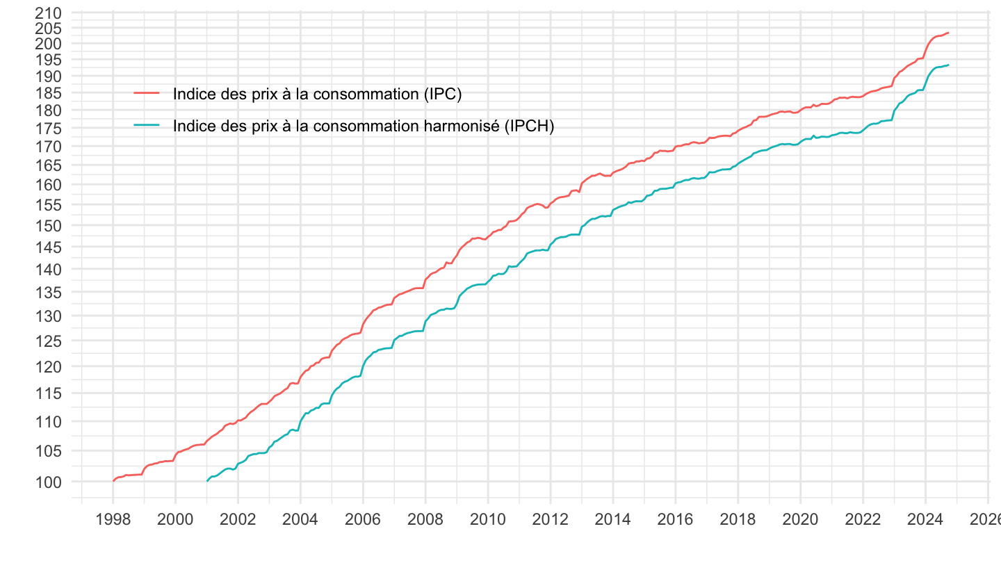
`IPCH-2015` |>
  bind_rows(`IPC-2015`) |>
  filter(COICOP2016 %in% c("12403"),
         NATURE == "INDICE",
         REF_AREA == "FE",
         FREQ == "M",
         is.na(MENAGES_IPC) | MENAGES_IPC == "ENSEMBLE") |>
  month_to_date() |>

  group_by(INDICATEUR) |>
  filter(date >= as.Date("1996-01-01")) |>
  arrange(date) |>
  mutate(OBS_VALUE = 100*OBS_VALUE/OBS_VALUE[1]) |>
  ggplot() + ylab("") + xlab("") + theme_minimal() +
  geom_line(aes(x = date, y = OBS_VALUE, color = Indicateur)) +

  scale_x_date(breaks = seq(1920, 2100, 2) |> paste0("-01-01") |> as.Date(),
               labels = date_format("%Y")) +
  theme(legend.position = c(0.3, 0.8),
        legend.title = element_blank()) +
  scale_y_log10(breaks = seq(10, 300, 5),
                     labels = dollar_format(accuracy = 1, prefix = ""))
| source | dataset | Title | Updated |
|---|---|---|---|
| source | dataset | Title | Updated |
|---|---|---|---|
| source | dataset | Title | Updated |
|---|---|---|---|


