
Last observation: 31 déc. 2026 (N = 2) · 9 oct. 2026 (N = 13) · sept. 2026 (N = 18)
First observation: janv. 1980 (N = 4) · 2 janv. 1990 (N = 1) · 30 juin 2015 (N = 2)
Last data update: 09 oct. 2026, 22:01
Last compile: 09 oct. 2026, 23:56
FM |>
  filter(grepl("FM.D.U2.EUR.4F.KR.MRR_FR.LEV", variable) |
           grepl("FM.D.U2.EUR.4F.KR.MLFR.LEV", variable) |
           grepl("FM.D.U2.EUR.4F.KR.DFR.LEV", variable)) |>

  ggplot() + geom_line(aes(x = date, y = value/100, color = Variable)) +

  theme_minimal() + xlab("") + ylab("Taux d'intérêt (%)") +
  scale_x_date(breaks = as.Date(paste0(seq(1960,2100, 5), "-01-01")),
               labels = date_format("%Y")) +
  theme(legend.position = c(0.35, 0.1),
        legend.title = element_blank(),
        legend.direction = "vertical") +
  scale_y_continuous(breaks = 0.01*seq(-10, 100, 1),
                labels = percent_format(accuracy = 1))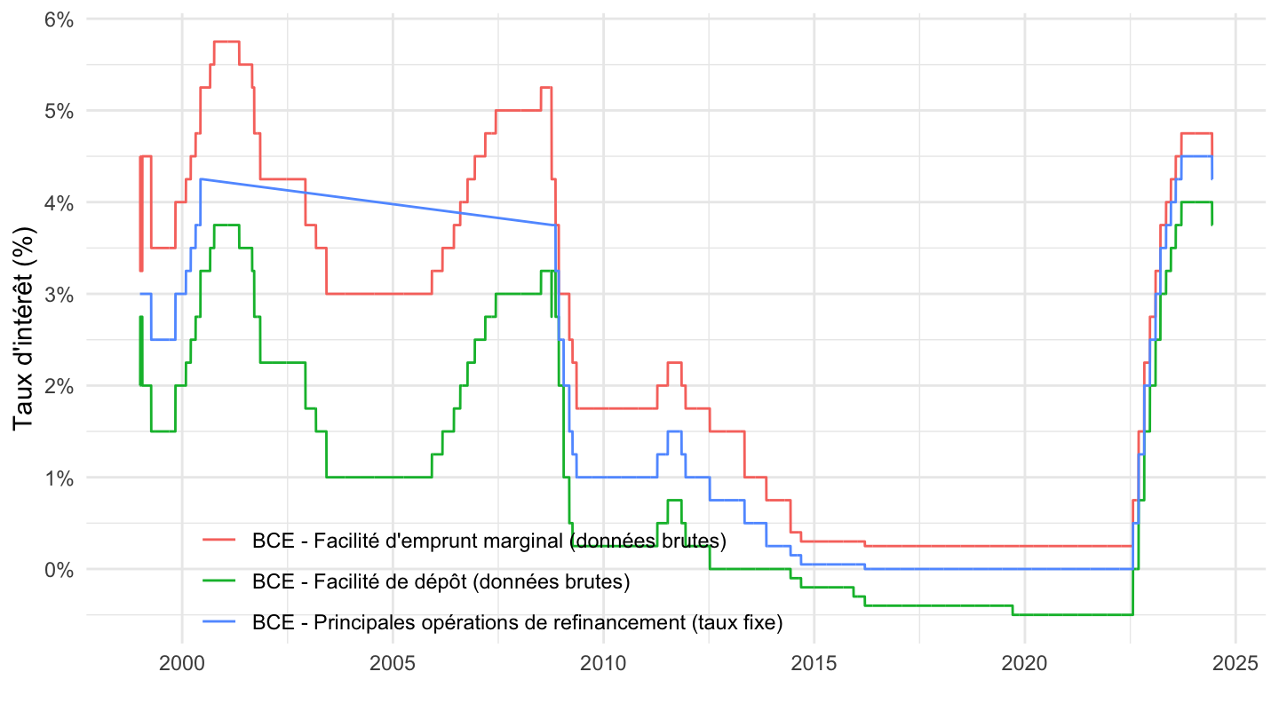
FM |>
  filter(grepl("FM.D.U2.EUR.4F.KR.MRR_FR.LEV", variable) |
           grepl("FM.D.U2.EUR.4F.KR.MLFR.LEV", variable) |
           grepl("FM.D.U2.EUR.4F.KR.DFR.LEV", variable)) |>
  filter(date >= as.Date("2022-01-01")) |>

  ggplot() + geom_line(aes(x = date, y = value/100, color = Variable)) +

  theme_minimal() + xlab("") + ylab("Taux d'intérêt (%)") +
  scale_x_date(breaks = "1 month",
               labels = date_format("%b %Y")) +
  theme(legend.position = c(0.3, 0.9),
        legend.title = element_blank(),
        legend.direction = "vertical",
        axis.text.x = element_text(angle = 45, vjust = 1, hjust = 1)) +
  scale_y_continuous(breaks = 0.01*seq(-10, 100, 1),
                labels = percent_format(accuracy = 1))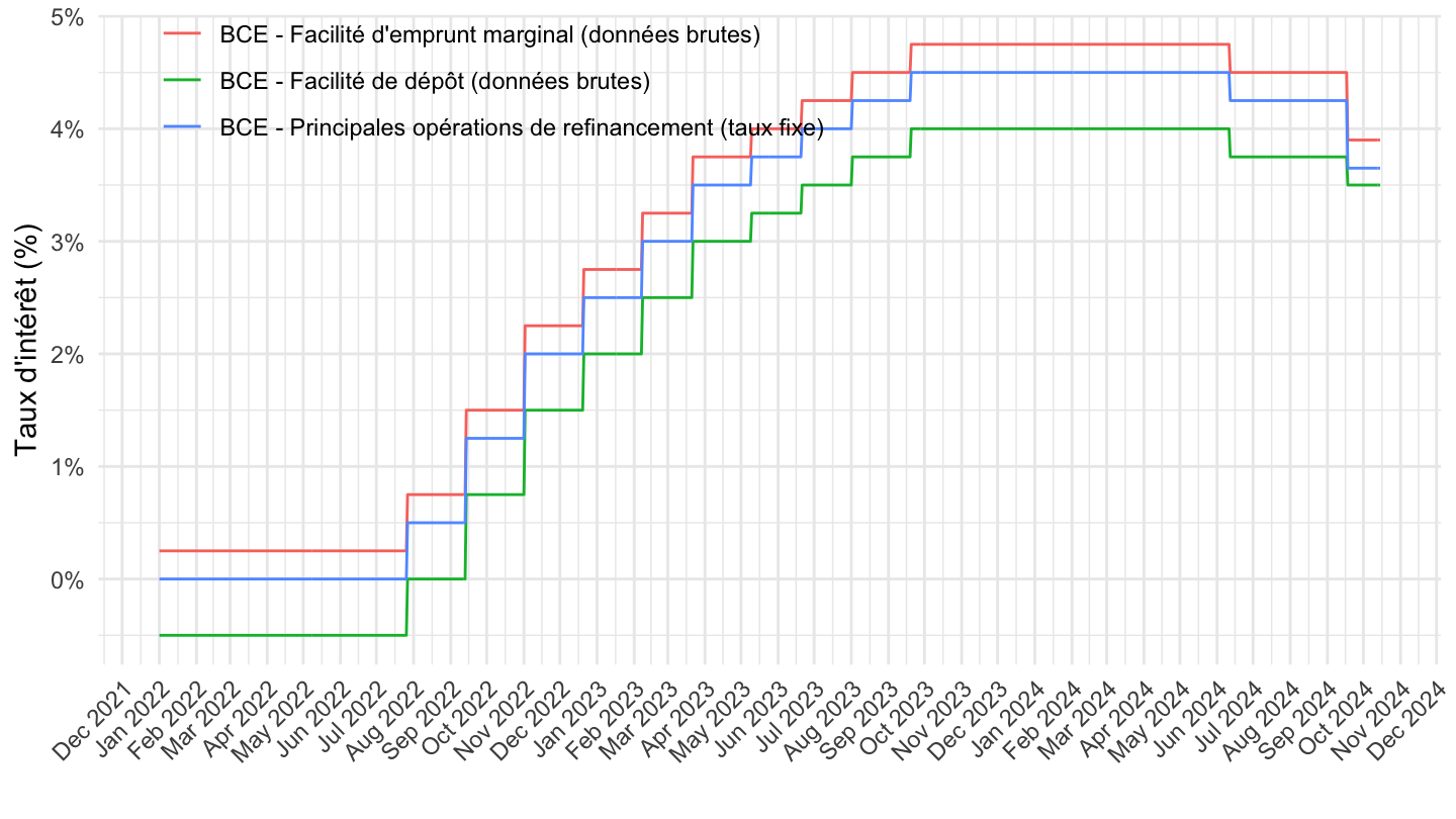
FM |>

  filter(PROVIDER_FM_ID %in% c("FRMOYTEC10", "FRMOYTEC5"),
          FREQ == "D") |>
  select_if(function(col) length(unique(col)) > 1) |>
  ggplot() + geom_line(aes(x = date, y = value/100, color = Variable)) +

  theme_minimal() + xlab("") + ylab("Taux d'intérêt (%)") +
  scale_x_date(breaks = as.Date(paste0(seq(1960,2100, 1), "-01-01")),
               labels = date_format("%Y")) +
  theme(legend.position = c(0.7, 0.9),
        legend.title = element_blank(),
        legend.direction = "vertical",
        axis.text.x = element_text(angle = 45, vjust = 1, hjust = 1)) +
  scale_y_continuous(breaks = 0.01*seq(-10, 100, .2),
                labels = percent_format(accuracy = .1)) +
  geom_hline(yintercept =  0, linetype = "dashed") +
  geom_label(data = . %>% filter(date == max(date)),
             aes(x = date, y = value/100, label = percent(value/100), color = Variable))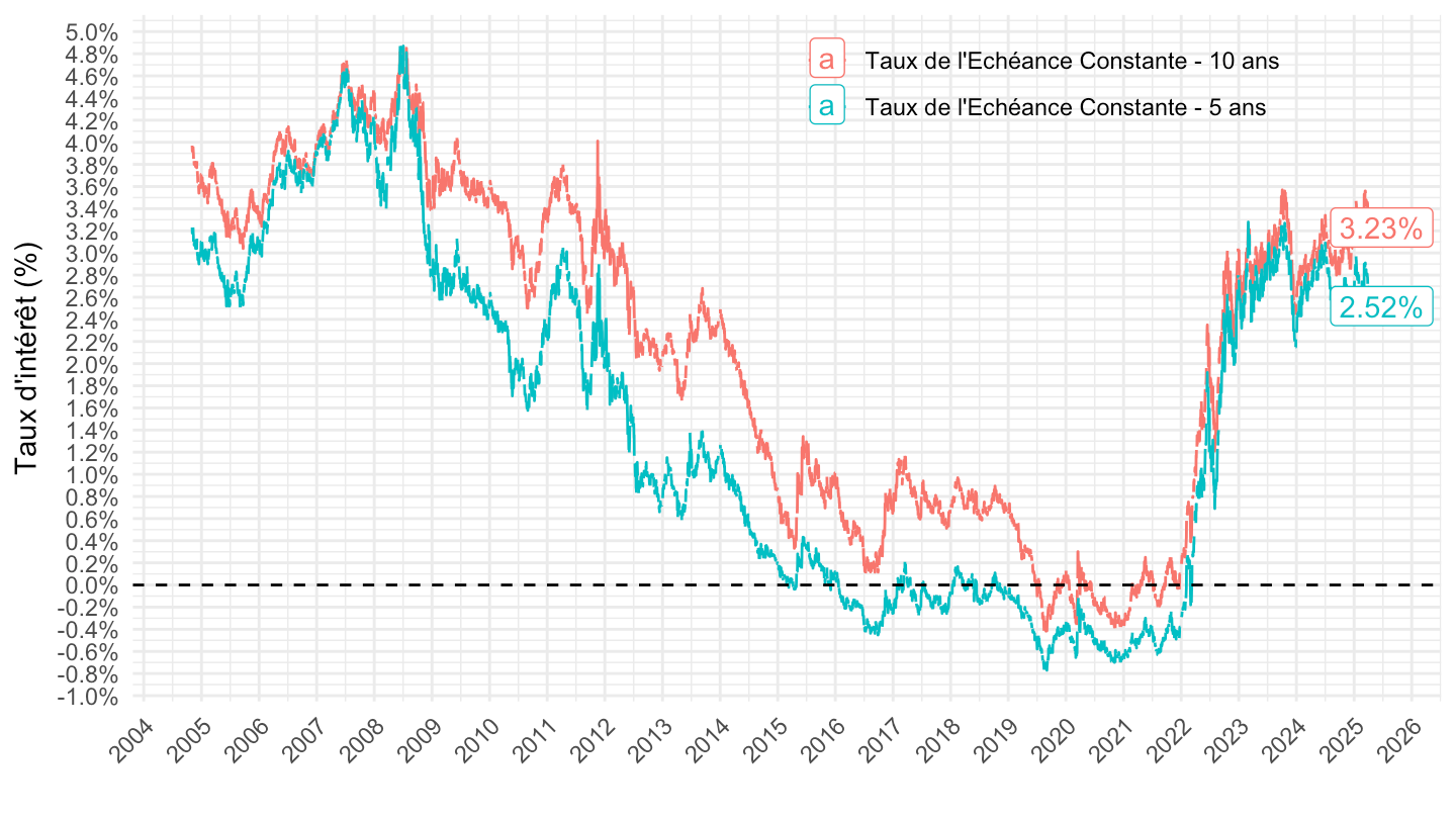
FM |>

  filter(PROVIDER_FM_ID %in% c("FRMOYTEC10", "FRMOYTEC5"),
         date >= as.Date("2018-01-01"),
          FREQ == "D") |>
  select_if(function(col) length(unique(col)) > 1) |>
  ggplot() + geom_line(aes(x = date, y = value/100, color = Variable)) +

  theme_minimal() + xlab("") + ylab("Taux d'intérêt (%)") +
  scale_x_date(breaks = as.Date(paste0(seq(1960,2100, 1), "-01-01")),
               labels = date_format("%Y")) +
  theme(legend.position = c(0.2, 0.9),
        legend.title = element_blank(),
        legend.direction = "vertical") +
  scale_y_continuous(breaks = 0.01*seq(-10, 100, .2),
                labels = percent_format(accuracy = .1)) +
  geom_hline(yintercept =  0, linetype = "dashed") +
  geom_label(data = . %>% filter(date == max(date)),
             aes(x = date, y = value/100, label = percent(value/100), color = Variable))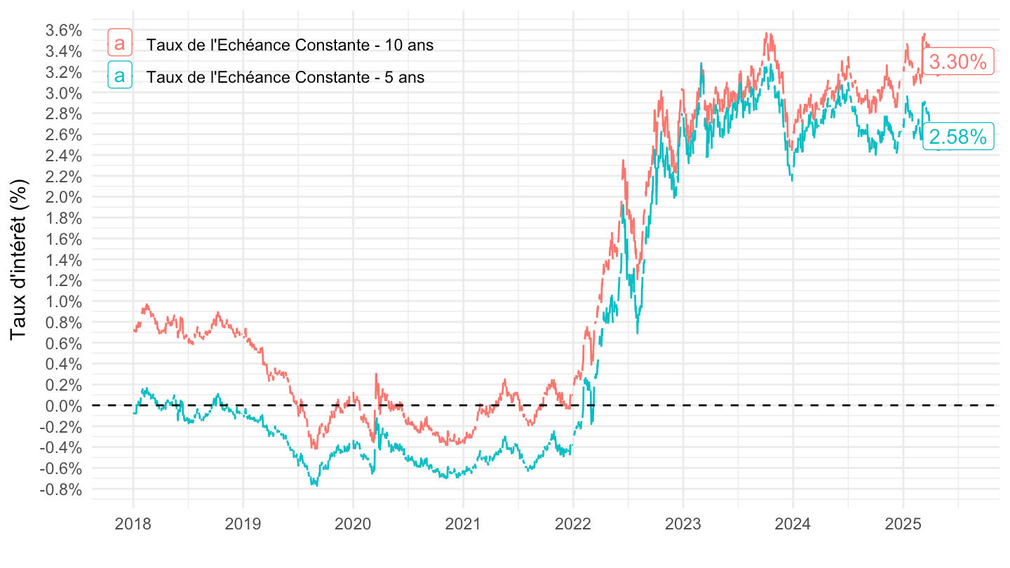
FM |>

  filter(PROVIDER_FM_ID %in% c("FRMOYTEC10", "FRMOYTEC5"),
         date >= as.Date("2020-01-01"),
          FREQ == "D") |>
  ggplot() + geom_line(aes(x = date, y = value/100, color = Variable)) +

  theme_minimal() + xlab("") + ylab("Taux d'intérêt (%)") +
  scale_x_date(breaks = "3 months",
               labels = date_format("%b %Y")) +
  theme(legend.position = c(0.2, 0.9),
        legend.title = element_blank(),
        legend.direction = "vertical",
        axis.text.x = element_text(angle = 45, vjust = 1, hjust = 1)) +
  scale_y_continuous(breaks = 0.01*seq(-10, 100, .2),
                labels = percent_format(accuracy = .1)) +
  geom_hline(yintercept =  0, linetype = "dashed") +
  geom_label(data = . %>% filter(date == max(date)),
             aes(x = date, y = value/100, label = percent(value/100), color = Variable))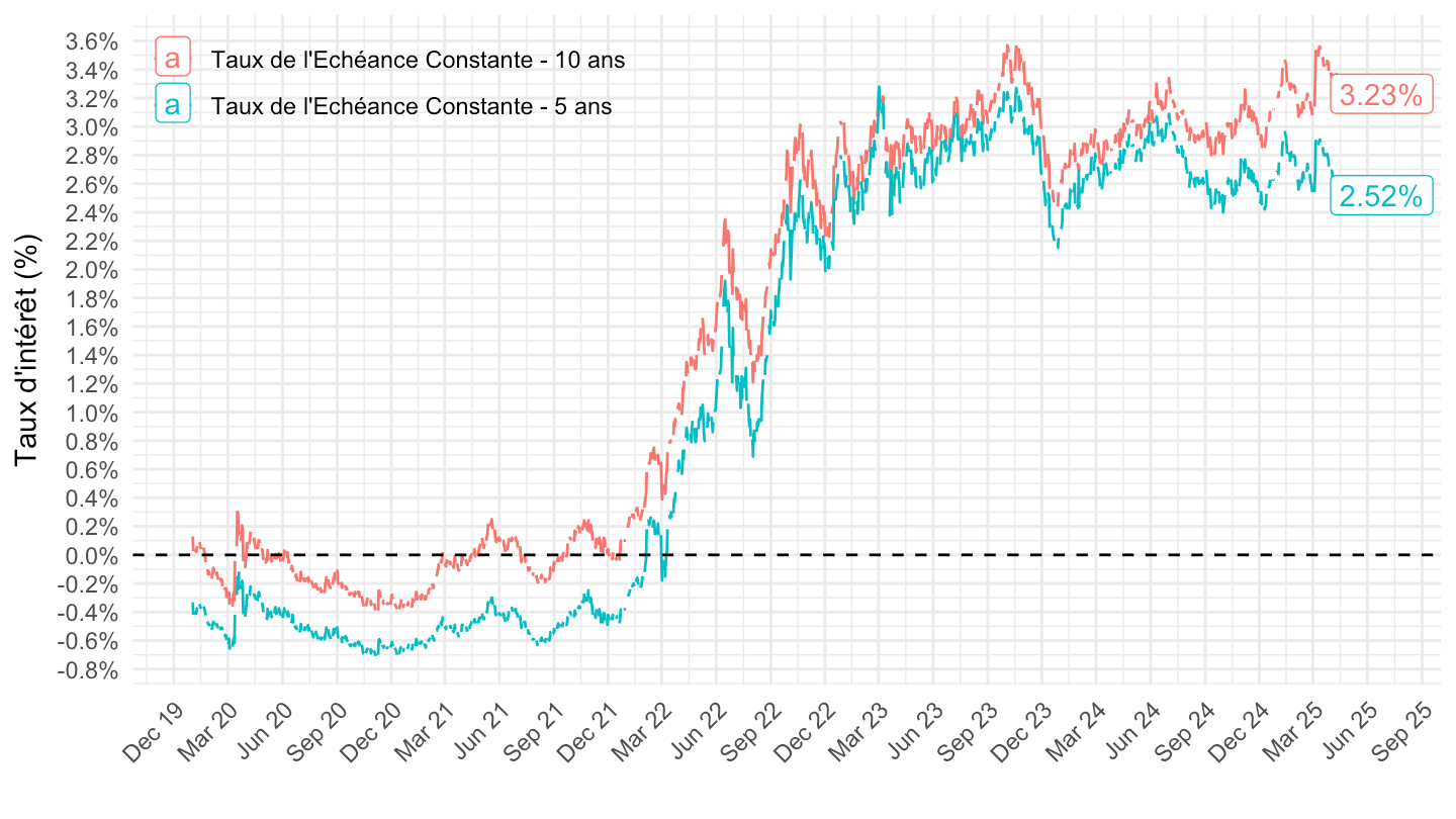
FM |>

  filter(PROVIDER_FM_ID %in% c("FRMOYTEC10", "FRMOYTEC5"),
         date >= as.Date("2021-01-01"),
          FREQ == "D") |>
  arrange(desc(date)) |>
  ggplot() + geom_line(aes(x = date, y = value/100, color = Variable)) +

  theme_minimal() + xlab("") + ylab("Taux d'intérêt (%)") +
  scale_x_date(breaks = "2 months",
               labels = date_format("%b %Y")) +
  theme(legend.position = c(0.2, 0.9),
        legend.title = element_blank(),
        legend.direction = "vertical",
        axis.text.x = element_text(angle = 45, vjust = 1, hjust = 1)) +
  scale_y_continuous(breaks = 0.01*seq(-10, 100, .2),
                labels = percent_format(accuracy = .1)) +
  geom_hline(yintercept =  0, linetype = "dashed") +
  geom_label(data = . %>% filter(date == max(date)),
             aes(x = date, y = value/100, label = percent(value/100), color = Variable))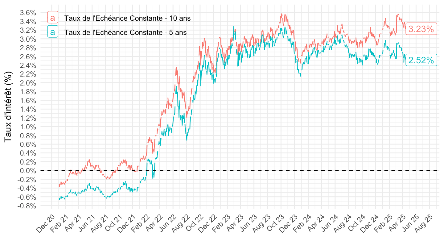
FM |>

  filter(PROVIDER_FM_ID %in% c("FRMOYTEC10", "FRMOYTEC5"),
         date >= Sys.Date() - years(2),
          FREQ == "D") |>
  arrange(desc(date)) |>
  ggplot() + geom_line(aes(x = date, y = value/100, color = Variable)) +

  theme_minimal() + xlab("") + ylab("Taux d'intérêt (%)") +
  scale_x_date(breaks = "1 month",
               labels = date_format("%b %Y")) +
  theme(legend.position = c(0.2, 0.9),
        legend.title = element_blank(),
        legend.direction = "vertical",
        axis.text.x = element_text(angle = 45, vjust = 1, hjust = 1)) +
  scale_y_continuous(breaks = 0.01*seq(-10, 100, .5),
                labels = percent_format(accuracy = .1)) +
  geom_hline(yintercept =  0, linetype = "dashed")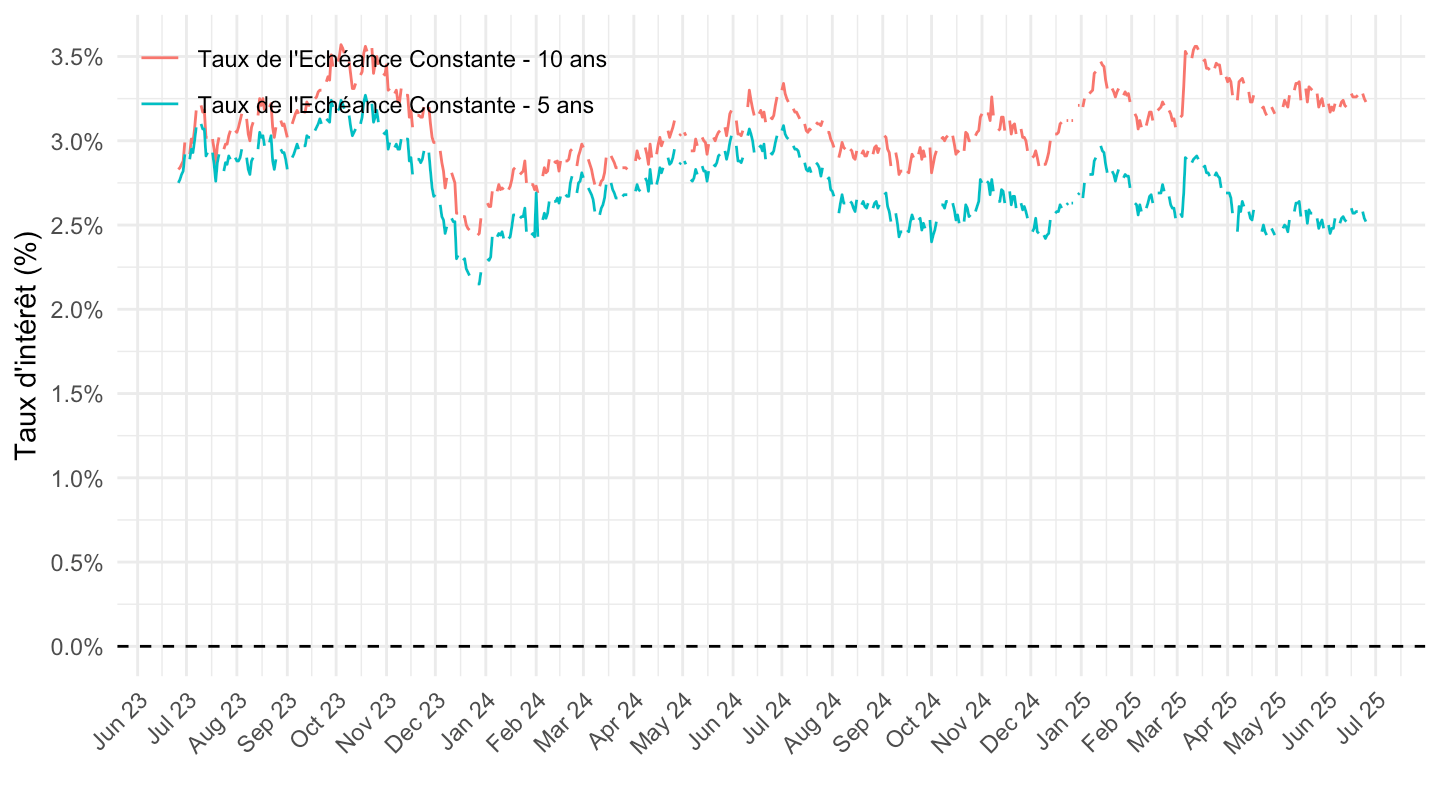
FM |>

  filter(PROVIDER_FM_ID %in% c("FRMOYTEC30", "FRMOYTEC10"),
         date >= as.Date("2018-01-01"),
          FREQ == "D") |>
  #select_if(function(col) length(unique(col)) > 1) %>%
  ggplot() + geom_line(aes(x = date, y = value/100, color = Variable)) +

  theme_minimal() + xlab("") + ylab("Taux d'intérêt (%)") +
  scale_x_date(breaks = as.Date(paste0(seq(1960,2100, 1), "-01-01")),
               labels = date_format("%Y")) +
  theme(legend.position = c(0.2, 0.9),
        legend.title = element_blank(),
        legend.direction = "vertical") +
  scale_y_continuous(breaks = 0.01*seq(-10, 100, .2),
                labels = percent_format(accuracy = .1)) +
  geom_hline(yintercept =  0, linetype = "dashed")
FM |>

  filter(PROVIDER_FM_ID %in% c("FRMOYTEC30"),
         date >= as.Date("2018-01-01"),
          FREQ == "D") |>
  #select_if(function(col) length(unique(col)) > 1) %>%
  ggplot() + geom_line(aes(x = date, y = value/100, color = Variable)) +

  theme_minimal() + xlab("") + ylab("Taux d'intérêt (%)") +
  scale_x_date(breaks = as.Date(paste0(seq(1960,2100, 1), "-01-01")),
               labels = date_format("%Y")) +
  theme(legend.position = c(0.2, 0.9),
        legend.title = element_blank(),
        legend.direction = "vertical") +
  scale_y_continuous(breaks = 0.01*seq(-10, 100, .2),
                labels = percent_format(accuracy = .1)) +
  geom_hline(yintercept =  0, linetype = "dashed")
FM |>

  filter(PROVIDER_FM_ID %in% c("FRMOYTEC10", "FRMOYTEC5", "FRMOYTEC30"),
         date >= as.Date("2018-01-01"),
          FREQ == "D") |>
  select_if(function(col) length(unique(col)) > 1) |>
  ggplot() + geom_line(aes(x = date, y = value/100, color = Variable)) +

  theme_minimal() + xlab("") + ylab("Taux d'intérêt (%)") +
  scale_x_date(breaks = as.Date(paste0(seq(1960,2100, 1), "-01-01")),
               labels = date_format("%Y")) +
  theme(legend.position = c(0.2, 0.9),
        legend.title = element_blank(),
        legend.direction = "vertical") +
  scale_y_continuous(breaks = 0.01*seq(-10, 100, .2),
                labels = percent_format(accuracy = .1)) +
  geom_hline(yintercept =  0, linetype = "dashed")
FM |>

  filter(PROVIDER_FM_ID %in% c("FRMOYTEC10", "FRMOYTEC5", "FRMOYTEC30"),
         date >= as.Date("2020-01-01"),
          FREQ == "D") |>
  ggplot() + geom_line(aes(x = date, y = value/100, color = Variable)) +

  theme_minimal() + xlab("") + ylab("Taux d'intérêt (%)") +
  scale_x_date(breaks = "3 months",
               labels = date_format("%b %Y")) +
  theme(legend.position = c(0.2, 0.9),
        legend.title = element_blank(),
        legend.direction = "vertical",
        axis.text.x = element_text(angle = 45, vjust = 1, hjust = 1)) +
  scale_y_continuous(breaks = 0.01*seq(-10, 100, .2),
                labels = percent_format(accuracy = .1)) +
  geom_hline(yintercept =  0, linetype = "dashed")
FM |>

  filter(PROVIDER_FM_ID %in% c("FRMOYTEC10", "FRMOYTEC5", "FRMOYTEC30"),
         date >= as.Date("2021-01-01"),
          FREQ == "D") |>
  arrange(desc(date)) |>
  ggplot() + geom_line(aes(x = date, y = value/100, color = Variable)) +

  theme_minimal() + xlab("") + ylab("Taux d'intérêt (%)") +
  scale_x_date(breaks = "2 months",
               labels = date_format("%b %Y")) +
  theme(legend.position = c(0.2, 0.9),
        legend.title = element_blank(),
        legend.direction = "vertical",
        axis.text.x = element_text(angle = 45, vjust = 1, hjust = 1)) +
  scale_y_continuous(breaks = 0.01*seq(-10, 100, .2),
                labels = percent_format(accuracy = .1)) +
  geom_hline(yintercept =  0, linetype = "dashed")
FM |>

  filter(PROVIDER_FM_ID %in% c("FRMOYTEC10", "FRMOYTEC5", "FRMOYTEC30"),
         date >= Sys.Date() - years(2),
          FREQ == "D") |>
  arrange(desc(date)) |>
  ggplot() + geom_line(aes(x = date, y = value/100, color = Variable)) +

  theme_minimal() + xlab("") + ylab("Taux d'intérêt (%)") +
  scale_x_date(breaks = "1 month",
               labels = date_format("%b %Y")) +
  theme(legend.position = c(0.2, 0.9),
        legend.title = element_blank(),
        legend.direction = "vertical",
        axis.text.x = element_text(angle = 45, vjust = 1, hjust = 1)) +
  scale_y_continuous(breaks = 0.01*seq(-10, 100, .5),
                labels = percent_format(accuracy = .1)) +
  geom_hline(yintercept =  0, linetype = "dashed")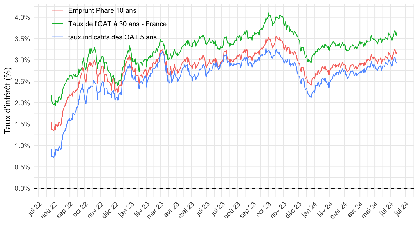
FM |>

  filter(PROVIDER_FM_ID %in% c("FRMOYTEC10", "FRMOYTEC5", "FRMOYTEC1"),
         date >= as.Date("2018-01-01"),
          FREQ == "D") |>
  select_if(function(col) length(unique(col)) > 1) |>
  ggplot() + geom_line(aes(x = date, y = value/100, color = Variable)) +

  theme_minimal() + xlab("") + ylab("Taux d'intérêt (%)") +
  scale_x_date(breaks = as.Date(paste0(seq(1960, 2030, 1), "-01-01")),
               labels = date_format("%Y")) +
  theme(legend.position = c(0.35, 0.9),
        legend.title = element_blank(),
        legend.direction = "vertical") +
  scale_y_continuous(breaks = 0.01*seq(-10, 100, .2),
                labels = percent_format(accuracy = .1)) +
  geom_hline(yintercept =  0, linetype = "dashed")
FM |>

  filter(PROVIDER_FM_ID %in% c("FRMOYTEC10", "FRMOYTEC5", "FRMOYTEC1"),
         date >= as.Date("2020-03-01"),
          FREQ == "D") |>
  ggplot() + geom_line(aes(x = date, y = value/100, color = Variable)) +

  theme_minimal() + xlab("") + ylab("Taux d'intérêt (%)") +
  scale_x_date(breaks = "3 months",
               labels = date_format("%b %Y")) +
  theme(legend.position = c(0.3, 0.9),
        legend.title = element_blank(),
        legend.direction = "vertical",
        axis.text.x = element_text(angle = 45, vjust = 1, hjust = 1)) +
  scale_y_continuous(breaks = 0.01*seq(-10, 100, .2),
                labels = percent_format(accuracy = .1)) +
  geom_hline(yintercept =  0, linetype = "dashed")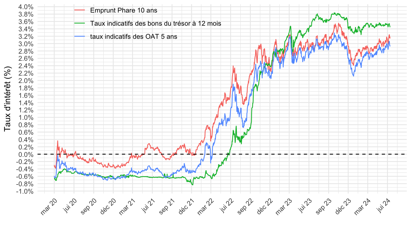
FM |>

  filter(PROVIDER_FM_ID %in% c("FRMOYTEC10", "FRMOYTEC5", "FRMOYTEC1"),
         date >= as.Date("2021-01-01"),
          FREQ == "D") |>
  arrange(desc(date)) |>
  ggplot() + geom_line(aes(x = date, y = value/100, color = Variable)) +

  theme_minimal() + xlab("") + ylab("Taux d'intérêt (%)") +
  scale_x_date(breaks = "2 months",
               labels = date_format("%b %Y")) +
  theme(legend.position = c(0.3, 0.9),
        legend.title = element_blank(),
        legend.direction = "vertical",
        axis.text.x = element_text(angle = 45, vjust = 1, hjust = 1)) +
  scale_y_continuous(breaks = 0.01*seq(-10, 100, .2),
                labels = percent_format(accuracy = .1)) +
  geom_hline(yintercept =  0, linetype = "dashed")
FM |>

  filter(PROVIDER_FM_ID %in% c("FRMOYTEC10", "FRMOYTEC5", "FRMOYTEC1"),
         date >= Sys.Date() - years(2),
          FREQ == "D") |>
  arrange(desc(date)) |>
  ggplot() + geom_line(aes(x = date, y = value/100, color = Variable)) +

  theme_minimal() + xlab("") + ylab("Taux d'intérêt (%)") +
  scale_x_date(breaks = "1 month",
               labels = date_format("%b %Y")) +
  theme(legend.position = c(0.25, 0.9),
        legend.title = element_blank(),
        legend.direction = "vertical",
        axis.text.x = element_text(angle = 45, vjust = 1, hjust = 1)) +
  scale_y_continuous(breaks = 0.01*seq(-10, 100, .5),
                labels = percent_format(accuracy = .1)) +
  geom_hline(yintercept =  0, linetype = "dashed")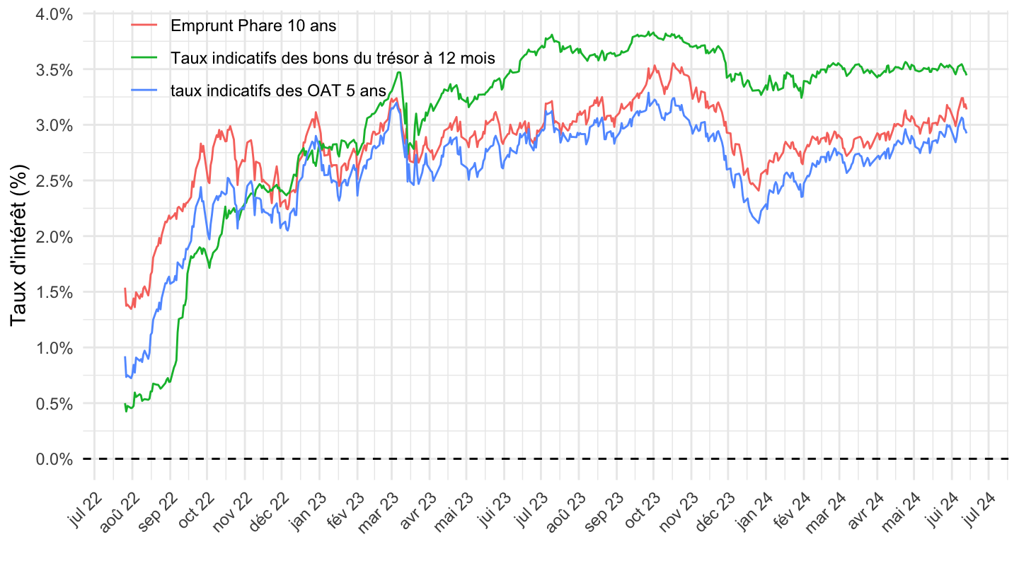
| source | dataset | Title | Updated |
|---|---|---|---|
| source | dataset | Title | Updated |
|---|---|---|---|
| source | dataset | Title | Updated |
|---|---|---|---|
| source | dataset | Title | Updated |
|---|---|---|---|





