| LAST_COMPILE |
|---|
| 2026-07-26 |
Consumer Price Index
Data - Fred
Info
LAST_COMPILE
Last
| date | Nobs |
|---|---|
| 2026-06-01 | 57 |
variable
All
Code
cpi %>%
  left_join(variable,  by = "variable") %>%
  group_by(variable, Variable) %>%
  summarise(Nobs = n()) %>%
  arrange(-Nobs) %>%
  print_table_conditional()
CBSA
Code
cpi %>%
  left_join(variable,  by = "variable") %>%
  filter(grepl("CBSA", Variable)) %>%
  group_by(variable, Variable) %>%
  summarise(Nobs = n()) %>%
  arrange(-Nobs) %>%
  {if (is_html_output()) datatable(., filter = 'top', rownames = F) else .}
Different Measures of inflation
PCE vs. CPI
Implicit Price Deflator - Imports of goods
All
Code
cpi %>%
  filter(variable == "A255RD3Q086SBEA") %>%
  ggplot() + ylab("Imports of goods (implicit price deflator)") + xlab("") + theme_minimal() +
  geom_line(aes(x = date, y = value)) +
  scale_x_date(breaks = seq(1920, 2100, 5) %>% paste0("-01-01") %>% as.Date,
               labels = date_format("%Y")) +
  theme(legend.position = c(0.75, 0.3),
        legend.title = element_blank()) +
  scale_y_log10(breaks = seq(0, 200, 10),
                     labels = dollar_format(accuracy = 1, prefix = ""))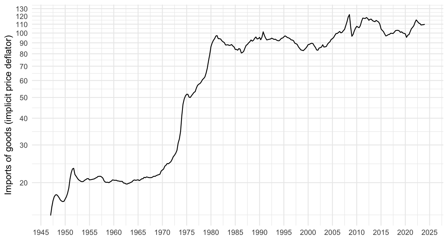
1980-
Code
cpi %>%
  filter(variable == "A255RD3Q086SBEA",
         date >= as.Date("1980-01-01")) %>%
  ggplot() + ylab("Imports of goods (implicit price deflator)") + xlab("") +
  theme_minimal() + geom_line(aes(x = date, y = value)) +
  scale_x_date(breaks = seq(1920, 2100, 5) %>% paste0("-01-01") %>% as.Date,
               labels = date_format("%Y")) +
  theme(legend.position = c(0.75, 0.3),
        legend.title = element_blank()) +
  scale_y_log10(breaks = seq(0, 200, 5),
                     labels = dollar_format(accuracy = 1, prefix = ""))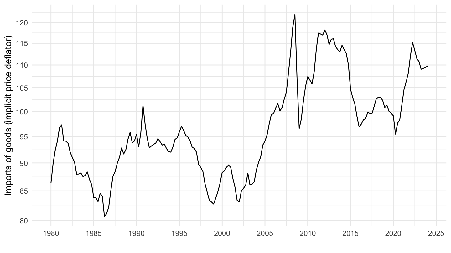
1990-
Code
cpi %>%
  filter(variable == "A255RD3Q086SBEA",
         date >= as.Date("1990-01-01")) %>%
  ggplot() + ylab("Imports of goods (implicit price deflator)") + xlab("") +
  theme_minimal() + geom_line(aes(x = date, y = value)) +
  scale_x_date(breaks = seq(1920, 2100, 5) %>% paste0("-01-01") %>% as.Date,
               labels = date_format("%Y")) +
  theme(legend.position = c(0.75, 0.3),
        legend.title = element_blank()) +
  scale_y_log10(breaks = seq(0, 200, 5),
                     labels = dollar_format(accuracy = 1, prefix = ""))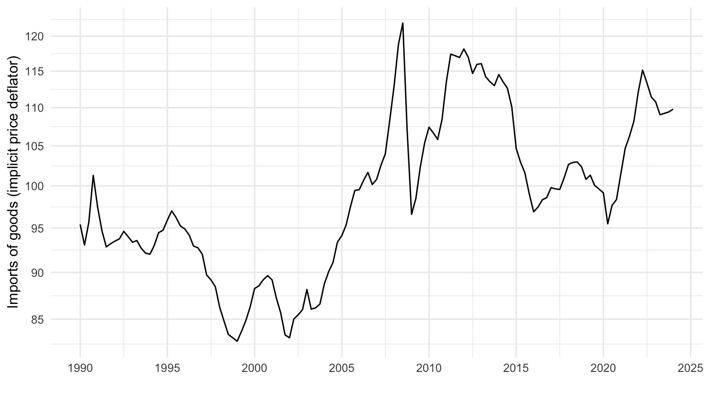
2000-
Code
cpi %>%
  filter(variable == "A255RD3Q086SBEA",
         date >= as.Date("2000-01-01")) %>%
  ggplot() + ylab("Imports of goods (implicit price deflator)") + xlab("") +
  theme_minimal() + geom_line(aes(x = date, y = value)) +
  scale_x_date(breaks = seq(1920, 2100, 2) %>% paste0("-01-01") %>% as.Date,
               labels = date_format("%Y")) +
  theme(legend.position = c(0.75, 0.3),
        legend.title = element_blank()) +
  scale_y_log10(breaks = seq(0, 200, 5),
                     labels = dollar_format(accuracy = 1, prefix = ""))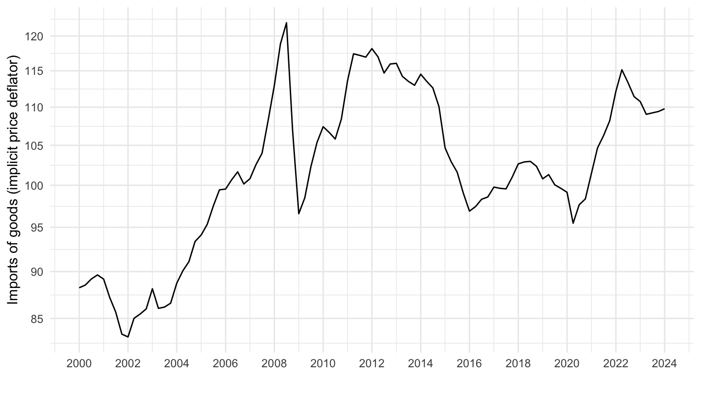
2010-
Code
cpi %>%
  filter(variable == "A255RD3Q086SBEA",
         date >= as.Date("2010-01-01")) %>%
  ggplot() + ylab("Imports of goods (implicit price deflator)") + xlab("") +
  theme_minimal() + geom_line(aes(x = date, y = value)) +
  scale_x_date(breaks = seq(1920, 2100, 5) %>% paste0("-01-01") %>% as.Date,
               labels = date_format("%Y")) +
  theme(legend.position = c(0.75, 0.3),
        legend.title = element_blank()) +
  scale_y_log10(breaks = seq(0, 200, 5),
                     labels = dollar_format(accuracy = 1, prefix = ""))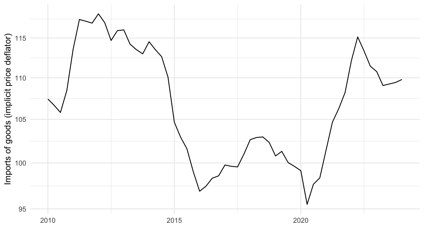
CPI
Linear
Code
plot_linear <- cpi %>%
  filter(variable %in% c("CPIAUCSL")) %>%
  ggplot + geom_line(aes(x = date, y = value)) +
  scale_y_continuous(breaks = seq(20, 500, 20)) +
  theme(legend.position = c(0.15, 0.85),
        legend.title = element_blank()) +
  scale_x_date(breaks = seq(1920, 2100, 10) %>% paste0("-01-01") %>% as.Date,
               labels = date_format("%Y")) +
  geom_rect(data = nber_recessions %>%
              filter(Peak >= as.Date("1946-01-01")),
            aes(xmin = Peak, xmax = Trough, ymin = 0, ymax = +Inf),
            fill = 'grey', alpha = 0.5) +
  theme_minimal() + labs(x = "", y = "")

plot_linear
Log
Code
plot_log <- plot_linear +
  scale_y_log10(breaks = c(10, 20, 30, 50, 80, 100, 150, 200, 300, 500, 1000))

plot_log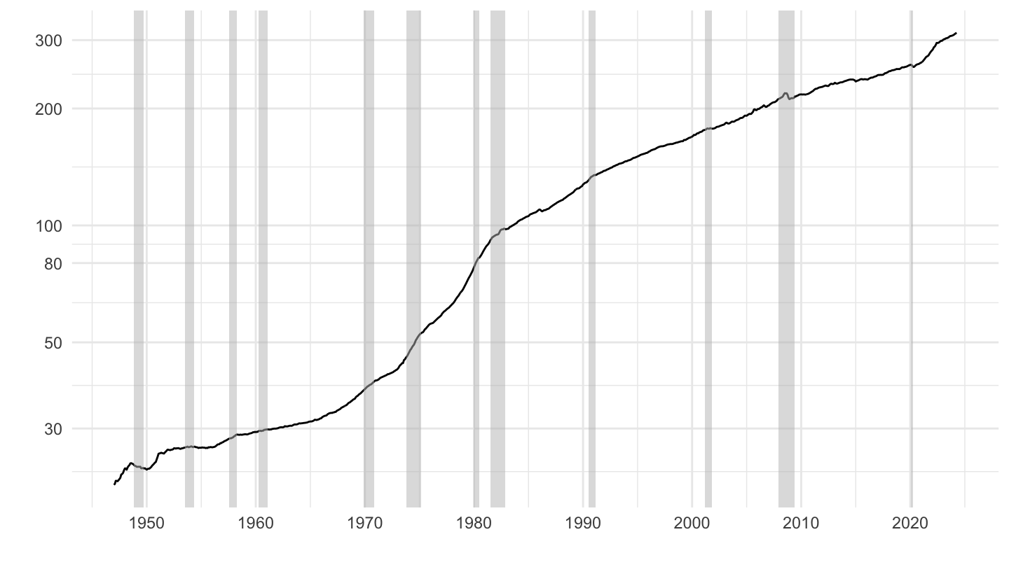
Bind
Code
ggpubr::ggarrange(plot_linear + ggtitle("Linear scale"), plot_log + ggtitle("Log scale"), common.legend = T)
U.S. CPI Components
1997 - 2019
Linear
Code
date0 <- as.Date("2019-03-01")
date1 <- as.Date("2020-12-01")
cpi %>%
  filter(variable %in% c("CUUR0000SEEB", "CPIAUCSL", "CPIMEDSL", "CUSR0000SERA02", "CUSR0000SEEA",
                         "CUUR0000SEMD", "CUSR0000SERE01", "CPIAPPSL", "CUUR0000SETA01", "CUUR0000SEHA"),
         date >= as.Date("1997-01-01")) %>%
  arrange(date) %>%
  group_by(variable) %>%
  mutate(value = 100 * value / value[1]) %>%
  ungroup %>%
  spread(variable, value) %>%
  ggplot(.) + scale_color_viridis(discrete = TRUE) +
  geom_line(color = viridis(10)[1], aes(x = date, y = CUUR0000SEEB)) +
  geom_text(data = . %>% filter(date == date0), color = viridis(10)[1], aes(x = date1, y = CUUR0000SEEB, label = "Tuition, childcare")) +
  geom_line(color = viridis(10)[2], linetype = 2, aes(x = date, y = CPIAUCSL)) +
  geom_text(data = . %>% filter(date == date0), color = viridis(10)[2], aes(x = date1, y = CPIAUCSL, label = "General Price Index")) +
  geom_line(color = viridis(10)[3], linetype = 3, aes(x = date, y = CPIMEDSL)) +
  geom_text(data = . %>% filter(date == date0), color = viridis(10)[3], aes(x = date1, y = CPIMEDSL, label = "Medical Care")) +
  geom_line(color = viridis(10)[4], linetype = 4, aes(x = date, y = CUSR0000SEEA)) +
  geom_text(data = . %>% filter(date == date0), color = viridis(10)[4], aes(x = date1, y = CUSR0000SEEA, label = "Educational Books")) +
  geom_line(color = viridis(10)[5], linetype = 5, aes(x = date, y = CUUR0000SEMD)) +
  geom_text(data = . %>% filter(date == date0), color = viridis(10)[5], aes(x = date1, y = CUUR0000SEMD, label = "Hospital Services")) +
  geom_line(color = viridis(10)[6], linetype = 6, aes(x = date, y = CUSR0000SERE01)) +
  geom_text(data = . %>% filter(date == date0), color = viridis(10)[6], aes(x = date1, y = CUSR0000SERE01, label = "Toys")) +
  geom_line(color = viridis(10)[7], linetype = 7, aes(x = date, y = CPIAPPSL)) +
  geom_text(data = . %>% filter(date == date0), color = viridis(10)[7], aes(x = date1, y = CPIAPPSL, label = "Apparel")) +
  geom_line(color = viridis(10)[8], linetype = 8, aes(x = date, y = CUUR0000SETA01)) +
  geom_text(data = . %>% filter(date == date0), color = viridis(10)[8], aes(x = date1, y = CUUR0000SETA01, label = "New vehicles")) +
  geom_line(color = viridis(10)[9], linetype = 9, aes(x = date, y = CUUR0000SEHA)) +
  geom_text(data = . %>% filter(date == date0), color = viridis(10)[9], aes(x = date1, y = CUUR0000SEHA, label = "Rents")) +
  scale_x_date(breaks = seq(1940, 2100, 2) %>% paste0("-01-01") %>% as.Date,
               labels = date_format("%Y"),
               limits = c(1997, 2025) %>% paste0("-01-01") %>% as.Date) +
  scale_y_continuous(breaks = seq(0, 600, 20)) +
  geom_rect(data = nber_recessions,
            aes(xmin = Peak, xmax = Trough, ymin = -Inf, ymax = +Inf),
            fill = 'grey', alpha = 0.5) +
  theme(legend.position = c(0.15, 0.85),
        legend.title = element_blank()) +
  theme_minimal() + labs(x = "", y = "")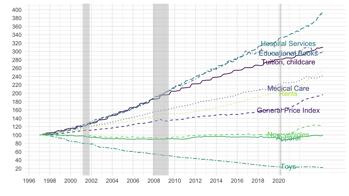
Log
Code
date0 <- as.Date("2019-03-01")
date1 <- as.Date("2020-12-01")
cpi %>%
  filter(variable %in% c("CUUR0000SEEB", "CPIAUCSL", "CPIMEDSL", "CUSR0000SERA02", "CUSR0000SEEA",
                         "CUUR0000SEMD", "CUSR0000SERE01", "CPIAPPSL", "CUUR0000SETA01", "CUUR0000SEHA"),
         date >= as.Date("1997-01-01")) %>%
  arrange(date) %>%
  group_by(variable) %>%
  mutate(value = 100 * value / value[1]) %>%
  ungroup %>%
  spread(variable, value) %>%
  ggplot(.) + scale_color_viridis(discrete = TRUE) +
  geom_line(color = viridis(10)[1], aes(x = date, y = CUUR0000SEEB)) +
  geom_text(data = . %>% filter(date == date0), color = viridis(10)[1], aes(x = date1, y = CUUR0000SEEB, label = "Tuition, childcare")) +
  geom_line(color = viridis(10)[2], linetype = 2, aes(x = date, y = CPIAUCSL)) +
  geom_text(data = . %>% filter(date == date0), color = viridis(10)[2], aes(x = date1, y = CPIAUCSL, label = "General Price Index")) +
  geom_line(color = viridis(10)[3], linetype = 3, aes(x = date, y = CPIMEDSL)) +
  geom_text(data = . %>% filter(date == date0), color = viridis(10)[3], aes(x = date1, y = CPIMEDSL, label = "Medical Care")) +
  geom_line(color = viridis(10)[4], linetype = 4, aes(x = date, y = CUSR0000SEEA)) +
  geom_text(data = . %>% filter(date == date0), color = viridis(10)[4], aes(x = date1, y = CUSR0000SEEA, label = "Educational Books")) +
  geom_line(color = viridis(10)[5], linetype = 5, aes(x = date, y = CUUR0000SEMD)) +
  geom_text(data = . %>% filter(date == date0), color = viridis(10)[5], aes(x = date1, y = CUUR0000SEMD, label = "Hospital Services")) +
  geom_line(color = viridis(10)[6], linetype = 6, aes(x = date, y = CUSR0000SERE01)) +
  geom_text(data = . %>% filter(date == date0), color = viridis(10)[6], aes(x = date1, y = CUSR0000SERE01, label = "Toys")) +
  geom_line(color = viridis(10)[7], linetype = 7, aes(x = date, y = CPIAPPSL)) +
  geom_text(data = . %>% filter(date == date0), color = viridis(10)[7], aes(x = date1, y = CPIAPPSL, label = "Apparel")) +
  geom_line(color = viridis(10)[8], linetype = 8, aes(x = date, y = CUUR0000SETA01)) +
  geom_text(data = . %>% filter(date == date0), color = viridis(10)[8], aes(x = date1, y = CUUR0000SETA01, label = "New vehicles")) +
  geom_line(color = viridis(10)[9], linetype = 9, aes(x = date, y = CUUR0000SEHA)) +
  geom_text(data = . %>% filter(date == date0), color = viridis(10)[9], aes(x = date1, y = CUUR0000SEHA, label = "Rents")) +
  scale_x_date(breaks = seq(1940, 2100, 2) %>% paste0("-01-01") %>% as.Date,
               labels = date_format("%Y"),
               limits = c(1997, 2025) %>% paste0("-01-01") %>% as.Date) +
  scale_y_log10(breaks = c(10, 20, 30, 40, 60, 80, 100, 150, 200, 250, 300, 500, 1000)) +
  geom_rect(data = nber_recessions,
            aes(xmin = Peak, xmax = Trough, ymin = -Inf, ymax = +Inf),
            fill = 'grey', alpha = 0.5) +
  theme(legend.position = c(0.15, 0.85),
        legend.title = element_blank()) +
  theme_minimal() + labs(x = "", y = "")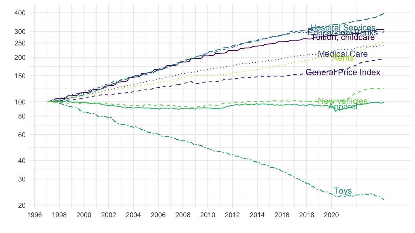
1977 - 2019
Linear
Code
date0 <- as.Date("2019-03-01")
date1 <- as.Date("2020-12-01")
cpi %>%
  filter(variable %in% c("CUUR0000SEEB", "CPIAUCSL", "CPIMEDSL", "CUSR0000SERA02", "CUSR0000SEEA",
                         "CUUR0000SEMD", "CUSR0000SERE01", "CPIAPPSL", "CUUR0000SETA01", "CUUR0000SEHA"),
         date >= as.Date("1977-01-01")) %>%
  arrange(date) %>%
  group_by(variable) %>%
  mutate(value = 100 * value / value[1]) %>%
  ungroup %>%
  spread(variable, value) %>%
  ggplot(.) + scale_color_viridis(discrete = TRUE) +
  geom_line(color = viridis(10)[1], aes(x = date, y = CUUR0000SEEB)) +
  geom_text(data = . %>% filter(date == date0), color = viridis(10)[1], aes(x = date1, y = CUUR0000SEEB, label = "Tuition, childcare")) +
  geom_line(color = viridis(10)[2], linetype = 2, aes(x = date, y = CPIAUCSL)) +
  geom_text(data = . %>% filter(date == date0), color = viridis(10)[2], aes(x = date1, y = CPIAUCSL, label = "General Price Index")) +
  geom_line(color = viridis(10)[3], linetype = 3, aes(x = date, y = CPIMEDSL)) +
  geom_text(data = . %>% filter(date == date0), color = viridis(10)[3], aes(x = date1, y = CPIMEDSL, label = "Medical Care")) +
  geom_line(color = viridis(10)[4], linetype = 4, aes(x = date, y = CUSR0000SEEA)) +
  geom_text(data = . %>% filter(date == date0), color = viridis(10)[4], aes(x = date1, y = CUSR0000SEEA, label = "Educational Books")) +
  geom_line(color = viridis(10)[5], linetype = 5, aes(x = date, y = CUUR0000SEMD)) +
  geom_text(data = . %>% filter(date == date0), color = viridis(10)[5], aes(x = date1, y = CUUR0000SEMD, label = "Hospital Services")) +
  geom_line(color = viridis(10)[6], linetype = 6, aes(x = date, y = CUSR0000SERE01)) +
  geom_text(data = . %>% filter(date == date0), color = viridis(10)[6], aes(x = date1, y = CUSR0000SERE01, label = "Toys")) +
  geom_line(color = viridis(10)[7], linetype = 7, aes(x = date, y = CPIAPPSL)) +
  geom_text(data = . %>% filter(date == date0), color = viridis(10)[7], aes(x = date1, y = CPIAPPSL, label = "Apparel")) +
  geom_line(color = viridis(10)[8], linetype = 8, aes(x = date, y = CUUR0000SETA01)) +
  geom_text(data = . %>% filter(date == date0), color = viridis(10)[8], aes(x = date1, y = CUUR0000SETA01, label = "New vehicles")) +
  geom_line(color = viridis(10)[9], linetype = 9, aes(x = date, y = CUUR0000SEHA)) +
  geom_text(data = . %>% filter(date == date0), color = viridis(10)[9], aes(x = date1, y = CUUR0000SEHA, label = "Rents")) +
  scale_x_date(breaks = seq(1940, 2100, 2) %>% paste0("-01-01") %>% as.Date,
               labels = date_format("%Y"),
               limits = c(1977, 2025) %>% paste0("-01-01") %>% as.Date) +
  scale_y_continuous(breaks = seq(0, 2000, 100)) +
  geom_rect(data = nber_recessions,
            aes(xmin = Peak, xmax = Trough, ymin = -Inf, ymax = +Inf),
            fill = 'grey', alpha = 0.5) +
  theme(legend.position = c(0.15, 0.85),
        legend.title = element_blank()) +
  theme_minimal() + labs(x = "", y = "")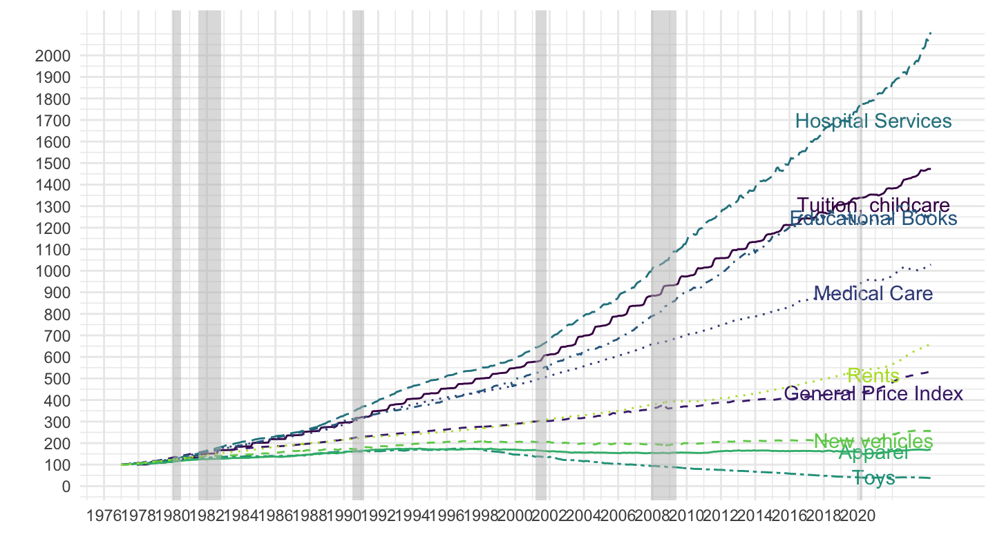
Log
Code
date0 <- as.Date("2019-03-01")
date1 <- as.Date("2020-12-01")
cpi %>%
  filter(variable %in% c("CUUR0000SEEB", "CPIAUCSL", "CPIMEDSL", "CUSR0000SERA02", "CUSR0000SEEA",
                         "CUUR0000SEMD", "CUSR0000SERE01", "CPIAPPSL", "CUUR0000SETA01", "CUUR0000SEHA"),
         date >= as.Date("1977-01-01")) %>%
  arrange(date) %>%
  group_by(variable) %>%
  mutate(value = 100 * value / value[1]) %>%
  ungroup %>%
  spread(variable, value) %>%
  ggplot(.) + scale_color_viridis(discrete = TRUE) +
  geom_line(color = viridis(10)[1], aes(x = date, y = CUUR0000SEEB)) +
  geom_text(data = . %>% filter(date == date0), color = viridis(10)[1], aes(x = date1, y = CUUR0000SEEB, label = "Tuition, childcare")) +
  geom_line(color = viridis(10)[2], linetype = 2, aes(x = date, y = CPIAUCSL)) +
  geom_text(data = . %>% filter(date == date0), color = viridis(10)[2], aes(x = date1, y = CPIAUCSL, label = "General Price Index")) +
  geom_line(color = viridis(10)[3], linetype = 3, aes(x = date, y = CPIMEDSL)) +
  geom_text(data = . %>% filter(date == date0), color = viridis(10)[3], aes(x = date1, y = CPIMEDSL, label = "Medical Care")) +
  geom_line(color = viridis(10)[4], linetype = 4, aes(x = date, y = CUSR0000SEEA)) +
  geom_text(data = . %>% filter(date == date0), color = viridis(10)[4], aes(x = date1, y = CUSR0000SEEA, label = "Educational Books")) +
  geom_line(color = viridis(10)[5], linetype = 5, aes(x = date, y = CUUR0000SEMD)) +
  geom_text(data = . %>% filter(date == date0), color = viridis(10)[5], aes(x = date1, y = CUUR0000SEMD, label = "Hospital Services")) +
  geom_line(color = viridis(10)[6], linetype = 6, aes(x = date, y = CUSR0000SERE01)) +
  geom_text(data = . %>% filter(date == date0), color = viridis(10)[6], aes(x = date1, y = CUSR0000SERE01, label = "Toys")) +
  geom_line(color = viridis(10)[7], linetype = 7, aes(x = date, y = CPIAPPSL)) +
  geom_text(data = . %>% filter(date == date0), color = viridis(10)[7], aes(x = date1, y = CPIAPPSL, label = "Apparel")) +
  geom_line(color = viridis(10)[8], linetype = 8, aes(x = date, y = CUUR0000SETA01)) +
  geom_text(data = . %>% filter(date == date0), color = viridis(10)[8], aes(x = date1, y = CUUR0000SETA01, label = "New vehicles")) +
  geom_line(color = viridis(10)[9], linetype = 9, aes(x = date, y = CUUR0000SEHA)) +
  geom_text(data = . %>% filter(date == date0), color = viridis(10)[9], aes(x = date1, y = CUUR0000SEHA, label = "Rents")) +
  scale_x_date(breaks = seq(1940, 2100, 2) %>% paste0("-01-01") %>% as.Date,
               labels = date_format("%Y"),
               limits = c(1977, 2025) %>% paste0("-01-01") %>% as.Date) +
  scale_y_log10(breaks = c(10, 20, 40, 80, 100, 200, 400, 800, 1000, 2000)) +
  geom_rect(data = nber_recessions,
            aes(xmin = Peak, xmax = Trough, ymin = -Inf, ymax = +Inf),
            fill = 'grey', alpha = 0.5) +
  theme(legend.position = c(0.15, 0.85),
        legend.title = element_blank()) +
  theme_minimal() + labs(x = "", y = "")
AFGAP Graph
- Association Française des Gestionnaires Actif-Passif - AFGAP. pdf
Code
date0 <- as.Date("2019-03-01")
date1 <- as.Date("2020-12-01")
cpi %>%
  filter(variable %in% c("CUUR0000SEEB", "CPIAUCSL", "CPIMEDSL", "CUSR0000SERA02", "CUSR0000SEEA",
                         "CUUR0000SEMD", "CUSR0000SERE01", "CPIAPPSL", "CUUR0000SETA01", "CUUR0000SEHA"),
         date >= as.Date("1977-01-01")) %>%
  arrange(date) %>%
  group_by(variable) %>%
  mutate(value = 100 * value / value[1]) %>%
  ungroup %>%
  spread(variable, value) %>%
  ggplot(.) + scale_color_viridis(discrete = TRUE) +
  geom_line(color = viridis(10)[1], aes(x = date, y = CUUR0000SEEB)) +
  geom_text(data = . %>% filter(date == date0), color = viridis(10)[1], aes(x = date1, y = CUUR0000SEEB, label = "Tuition, childcare")) +
  geom_line(color = viridis(10)[2], linetype = 2, aes(x = date, y = CPIAUCSL)) +
  geom_text(data = . %>% filter(date == date0), color = viridis(10)[2], aes(x = date1, y = CPIAUCSL, label = "General Price Index")) +
  geom_line(color = viridis(10)[3], linetype = 3, aes(x = date, y = CPIMEDSL)) +
  geom_text(data = . %>% filter(date == date0), color = viridis(10)[3], aes(x = date1, y = CPIMEDSL, label = "Medical Care")) +
  geom_line(color = viridis(10)[4], linetype = 4, aes(x = date, y = CUSR0000SEEA)) +
  geom_text(data = . %>% filter(date == date0), color = viridis(10)[4], aes(x = date1, y = CUSR0000SEEA, label = "Educational Books")) +
  geom_line(color = viridis(10)[5], linetype = 5, aes(x = date, y = CUUR0000SEMD)) +
  geom_text(data = . %>% filter(date == date0), color = viridis(10)[5], aes(x = date1, y = CUUR0000SEMD, label = "Hospital Services")) +
  geom_line(color = viridis(10)[6], linetype = 6, aes(x = date, y = CUSR0000SERE01)) +
  geom_text(data = . %>% filter(date == date0), color = viridis(10)[6], aes(x = date1, y = CUSR0000SERE01, label = "Toys")) +
  geom_line(color = viridis(10)[7], linetype = 7, aes(x = date, y = CPIAPPSL)) +
  geom_text(data = . %>% filter(date == date0), color = viridis(10)[7], aes(x = date1, y = CPIAPPSL, label = "Apparel")) +
  geom_line(color = viridis(10)[8], linetype = 8, aes(x = date, y = CUUR0000SETA01)) +
  geom_text(data = . %>% filter(date == date0), color = viridis(10)[8], aes(x = date1, y = CUUR0000SETA01, label = "New vehicles")) +
  geom_line(color = viridis(10)[9], linetype = 9, aes(x = date, y = CUUR0000SEHA)) +
  geom_text(data = . %>% filter(date == date0), color = viridis(10)[9], aes(x = date1, y = CUUR0000SEHA, label = "Rents")) +
  scale_x_date(breaks = seq(1940, 2100, 2) %>% paste0("-01-01") %>% as.Date,
               labels = date_format("%Y"),
               limits = c(1977, 2025) %>% paste0("-01-01") %>% as.Date) +
  scale_y_log10(breaks = c(10, 20, 40, 80, 100, 200, 400, 800, 1000, 2000)) +
  geom_rect(data = nber_recessions,
            aes(xmin = Peak, xmax = Trough, ymin = -Inf, ymax = +Inf),
            fill = 'grey', alpha = 0.5) +
  theme(legend.position = c(0.15, 0.85),
        legend.title = element_blank()) +
  theme_minimal() + labs(x = "", y = "")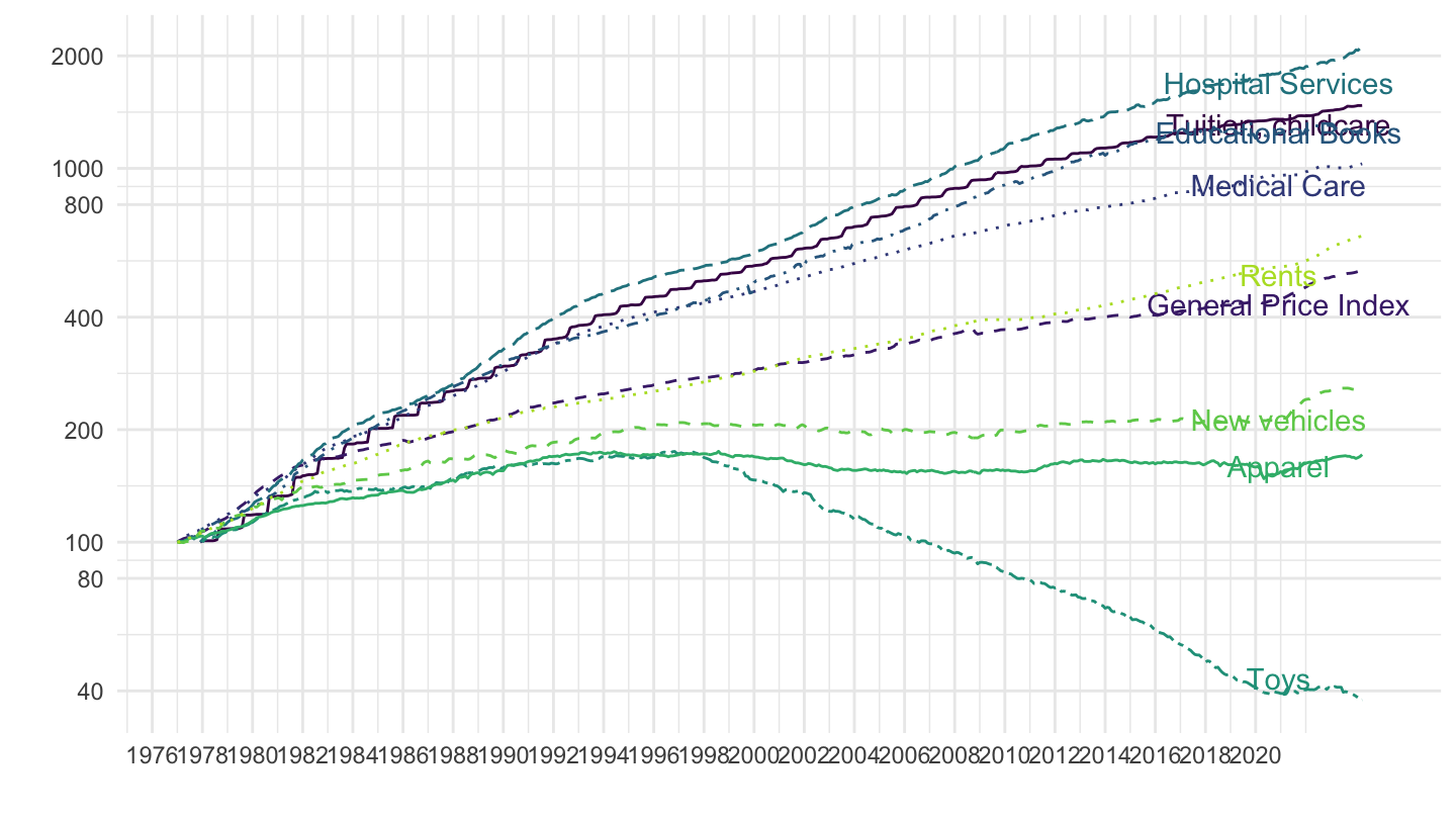
U.S. General Price Index
1913 - 1935
Code
cpi %>%
  filter(variable == "CPIAUCNS",
         date >= as.Date("1913-01-01"),
         date <= as.Date("1935-01-01"))  %>%
  ggplot(.) +
  geom_line(aes(x = date, y = value)) +
  ylab("CPI") + xlab("") +
  geom_rect(data = nber_recessions,
            aes(xmin = Peak, xmax = Trough, ymin = 0, ymax = +Inf),
            fill = 'grey', alpha = 0.5) +
  scale_y_log10(breaks = seq(1, 30, 1)) +
  scale_x_date(breaks = as.Date(paste0(seq(1913, 1935, 1), "-01-01")),
               labels = date_format("%Y"),
               limits = c(as.Date("1913-01-01"), as.Date("1935-01-01"))) +
  theme_minimal() +
  geom_vline(xintercept = as.Date("1929-10-29"), linetype = "dashed", color = viridis(3)[2])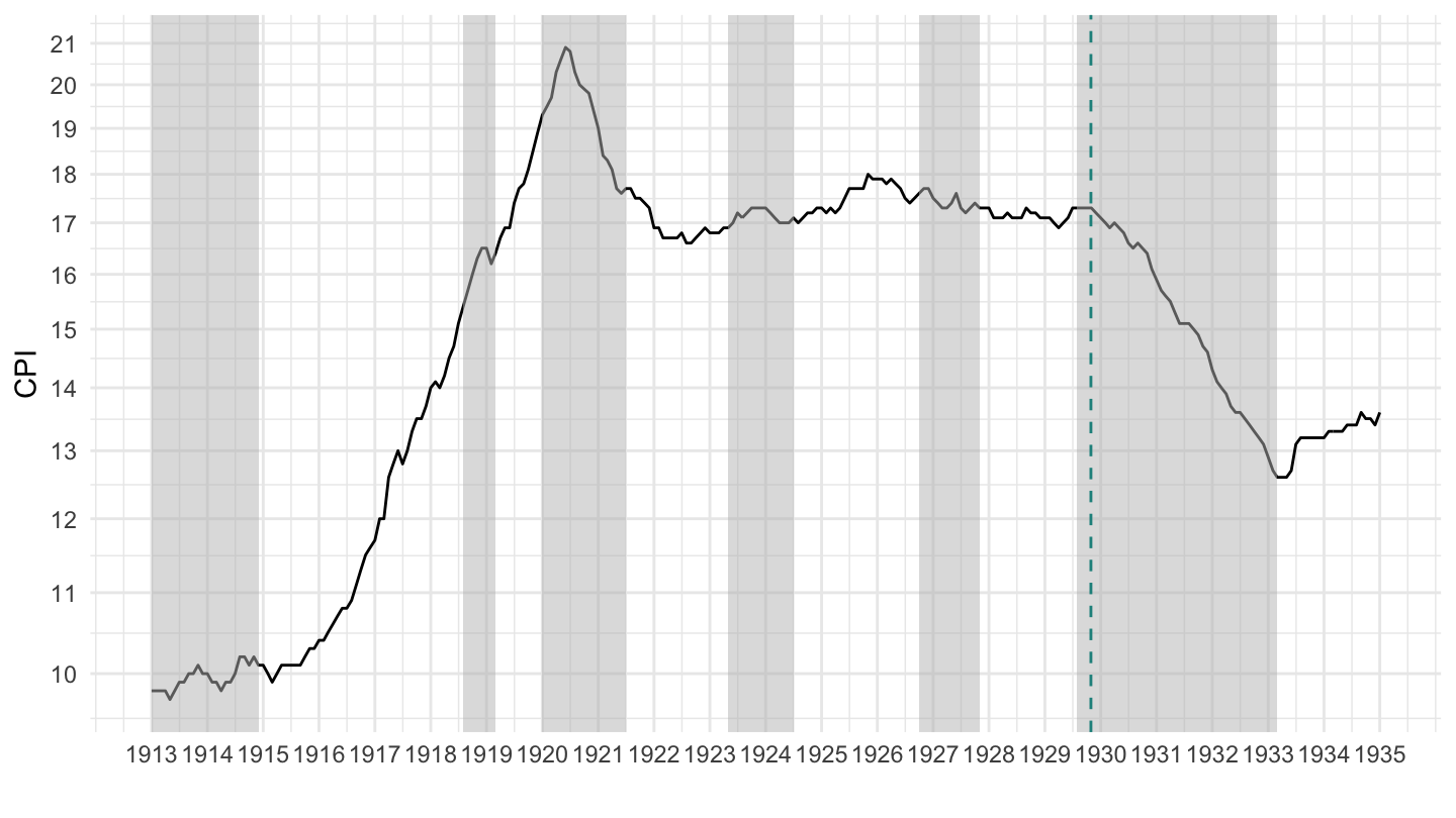
1913 - 1935
Code
cpi %>%
  filter(variable == "CPIAUCNS",
         date >= as.Date("1913-01-01"),
         date <= as.Date("1945-01-01"))  %>%
  ggplot(.) +
  geom_line(aes(x = date, y = value)) +
  ylab("CPI") + xlab("") +
  geom_rect(data = nber_recessions,
            aes(xmin = Peak, xmax = Trough, ymin = 0, ymax = +Inf),
            fill = 'grey', alpha = 0.5) +
  scale_y_log10(breaks = seq(1, 30, 1)) +
  scale_x_date(breaks = as.Date(paste0(seq(1910, 1945, 5), "-01-01")),
               labels = date_format("%Y"),
               limits = c(as.Date("1913-01-01"), as.Date("1945-01-01"))) +
  theme_minimal() +
  geom_vline(xintercept = as.Date("1929-10-29"), linetype = "dashed", color = viridis(3)[2])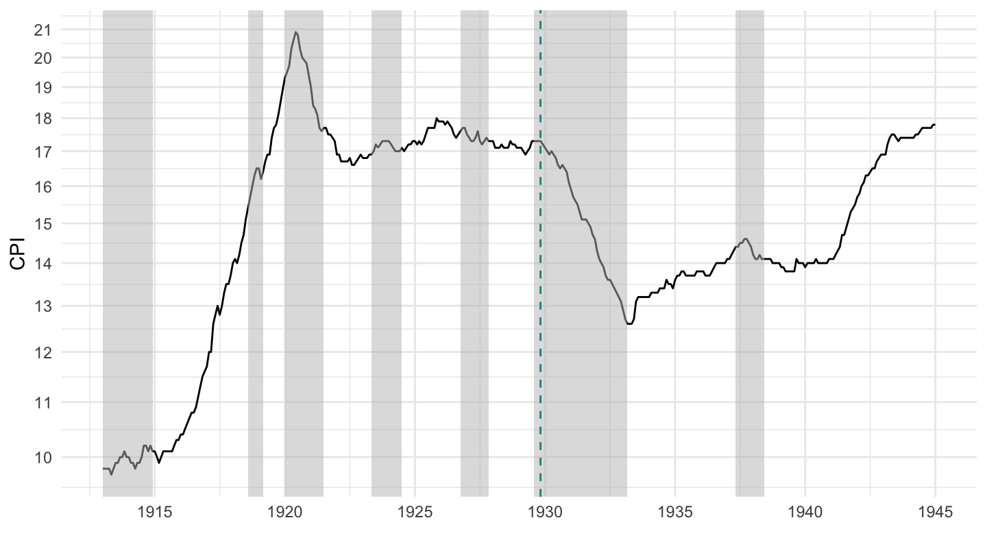
1922 - 1935
(ref:us-index-cpi) U.S. CPI (1922-1935)
Code
cpi %>%
  filter(variable == "CPIAUCNS",
         date >= as.Date("1922-01-01"),
         date <= as.Date("1935-01-01"))  %>%
  ggplot(.) +
  geom_line(aes(x = date, y = value)) +
  ylab("CPI") + xlab("") +
  geom_rect(data = nber_recessions,
            aes(xmin = Peak, xmax = Trough, ymin = 0, ymax = +Inf),
            fill = 'grey', alpha = 0.5) +
  scale_y_log10(breaks = seq(12, 18, 1),
                     limits = c(12, 18.5)) +
  scale_x_date(breaks = as.Date(paste0(seq(1922, 1935, 1), "-01-01")),
               labels = date_format("%Y"),
               limits = c(as.Date("1922-01-01"), as.Date("1935-01-01"))) +
  theme_minimal() +
  geom_vline(xintercept = as.Date("1929-10-29"), linetype = "dashed", color = viridis(3)[2])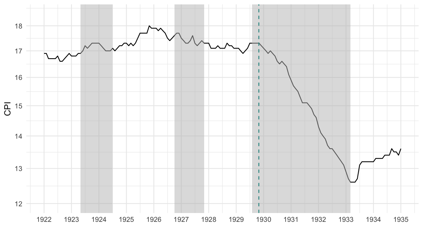
1860 - 1939
(ref:us-general-price-1860-1939) U.S. Index of the General Price Level (January 1860 - November 1939)
Code
cpi %>%
  filter(variable == "M04051USM324NNBR") %>%
  ggplot(.) +
  geom_line(aes(x = date, y = value)) +
  ylab("CPI") + xlab("") +
  geom_rect(data = nber_recessions,
            aes(xmin = Peak, xmax = Trough, ymin = -Inf, ymax = +Inf),
            fill = 'grey', alpha = 0.5) +
  scale_y_continuous(breaks = seq(50, 200, 10)) +
  scale_x_date(breaks = as.Date(paste0(seq(1860, 1939, 10), "-01-01")),
               labels = date_format("%Y"),
               limits = c(as.Date("1860-01-01"), as.Date("1939-01-01"))) +
  theme_minimal() +
  geom_vline(xintercept = as.Date("1929-10-29"), linetype = "dashed", color = "red")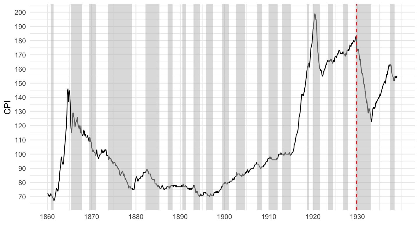
1903 - 1925
(ref:us-P-1903-1925-fisher) U.S. Index of the General Price Level (1903-1925)
Code
cpi %>%
  filter(variable == "M04051USM324NNBR") %>%
  filter(date >= as.Date("1903-01-01"), date <= as.Date("1925-01-01")) %>%
  ggplot(.) +
  geom_line(aes(x = date, y = value)) +
  ylab("CPI") + xlab("") +
  geom_rect(data = nber_recessions,
            aes(xmin = Peak, xmax = Trough, ymin = -Inf, ymax = +Inf),
            fill = 'grey', alpha = 0.5) +
  scale_y_continuous(breaks = seq(50, 200, 10)) +
  scale_x_date(breaks = as.Date(paste0(seq(1860, 1939, 5), "-01-01")),
               labels = date_format("%Y"),
               limits = c(as.Date("1903-01-01"), as.Date("1925-01-01"))) +
  theme_minimal() +
  geom_vline(xintercept = as.Date("1929-10-29"), linetype = "dashed", color = "red")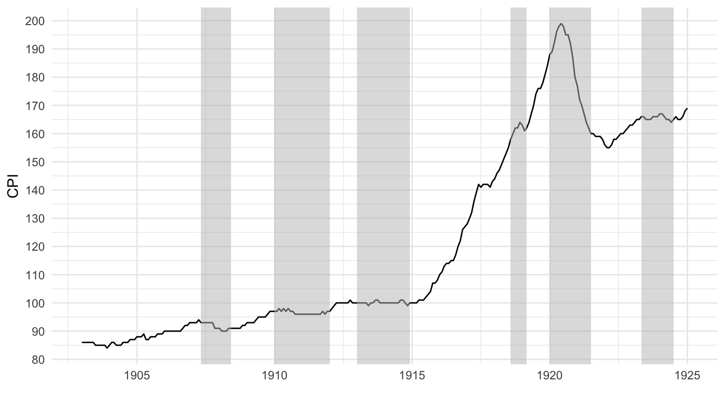
Case-Shiller - Fred
1986-
Log
Code
cpi %>%
  filter(variable == "CSUSHPINSA")  %>%
  na.omit %>%
  ggplot(.) + ylab("U.S. Case Shiller Price Index") + xlab("") + theme_minimal() +
  geom_line(aes(x = date, y = value)) +
  geom_rect(data = nber_recessions %>%
              filter(Peak >= as.Date("1987-01-01")),
            aes(xmin = Peak, xmax = Trough, ymin = 0, ymax = +Inf),
            fill = 'grey', alpha = 0.5) +
  scale_y_log10(breaks = seq(25, 1000, 25)) +
  scale_x_date(breaks = as.Date(paste0(seq(1900, 2022, 5), "-01-01")),
               labels = date_format("%Y"))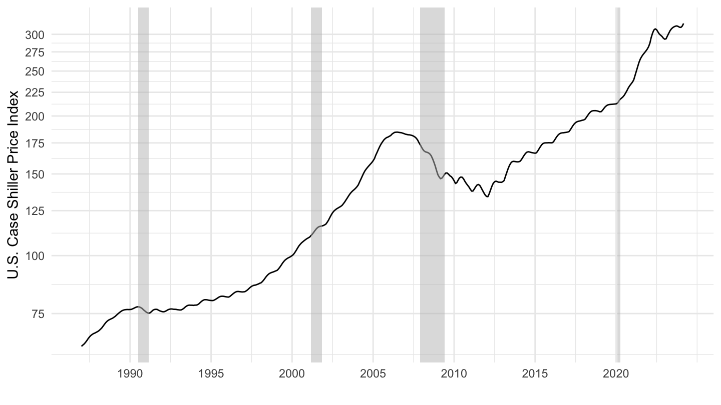
Linear
Code
cpi %>%
  filter(variable == "CSUSHPINSA")  %>%
  na.omit %>%
  ggplot(.) + ylab("U.S. Case Shiller Price Index") + xlab("") + theme_minimal() +
  geom_line(aes(x = date, y = value)) +
  geom_rect(data = nber_recessions %>%
              filter(Peak >= as.Date("1987-01-01")),
            aes(xmin = Peak, xmax = Trough, ymin = 0, ymax = +Inf),
            fill = 'grey', alpha = 0.5) +
  scale_y_continuous(breaks = seq(25, 1000, 25)) +
  scale_x_date(breaks = as.Date(paste0(seq(1900, 2022, 5), "-01-01")),
               labels = date_format("%Y"))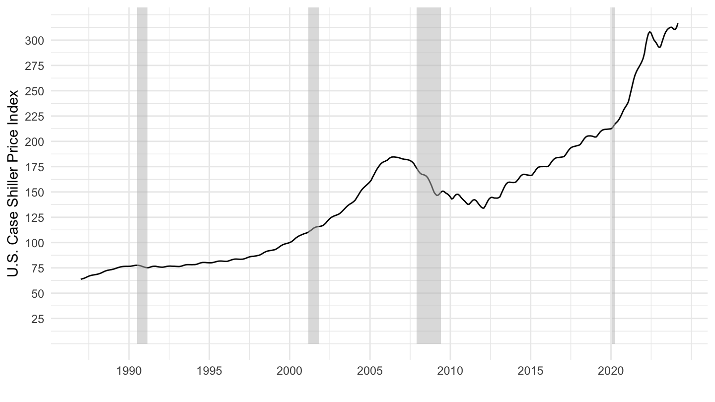
2000-
Code
cpi %>%
  filter(variable == "CSUSHPINSA",
         date >= as.Date("2000-01-01"))  %>%
  na.omit %>%
  ggplot(.) + ylab("U.S. Case Shiller Price Index") + xlab("") + theme_minimal() +
  geom_line(aes(x = date, y = value)) +
  geom_rect(data = nber_recessions %>%
              filter(Peak >= as.Date("2000-01-01")),
            aes(xmin = Peak, xmax = Trough, ymin = 0, ymax = +Inf),
            fill = 'grey', alpha = 0.5) +
  scale_y_log10(breaks = seq(10, 1000, 10)) +
  scale_x_date(breaks = as.Date(paste0(seq(1900, 2100, 2), "-01-01")),
               labels = date_format("%Y"))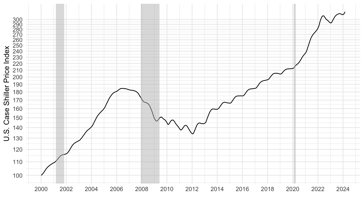
2010-
Code
cpi %>%
  filter(variable == "CSUSHPINSA",
         date >= as.Date("2010-01-01"))  %>%
  na.omit %>%
  ggplot(.) + ylab("U.S. Case Shiller Price Index") + xlab("") + theme_minimal() +
  geom_line(aes(x = date, y = value)) +
  scale_y_log10(breaks = seq(10, 1000, 10)) +
  scale_x_date(breaks = as.Date(paste0(seq(1900, 2100, 1), "-01-01")),
               labels = date_format("%Y"))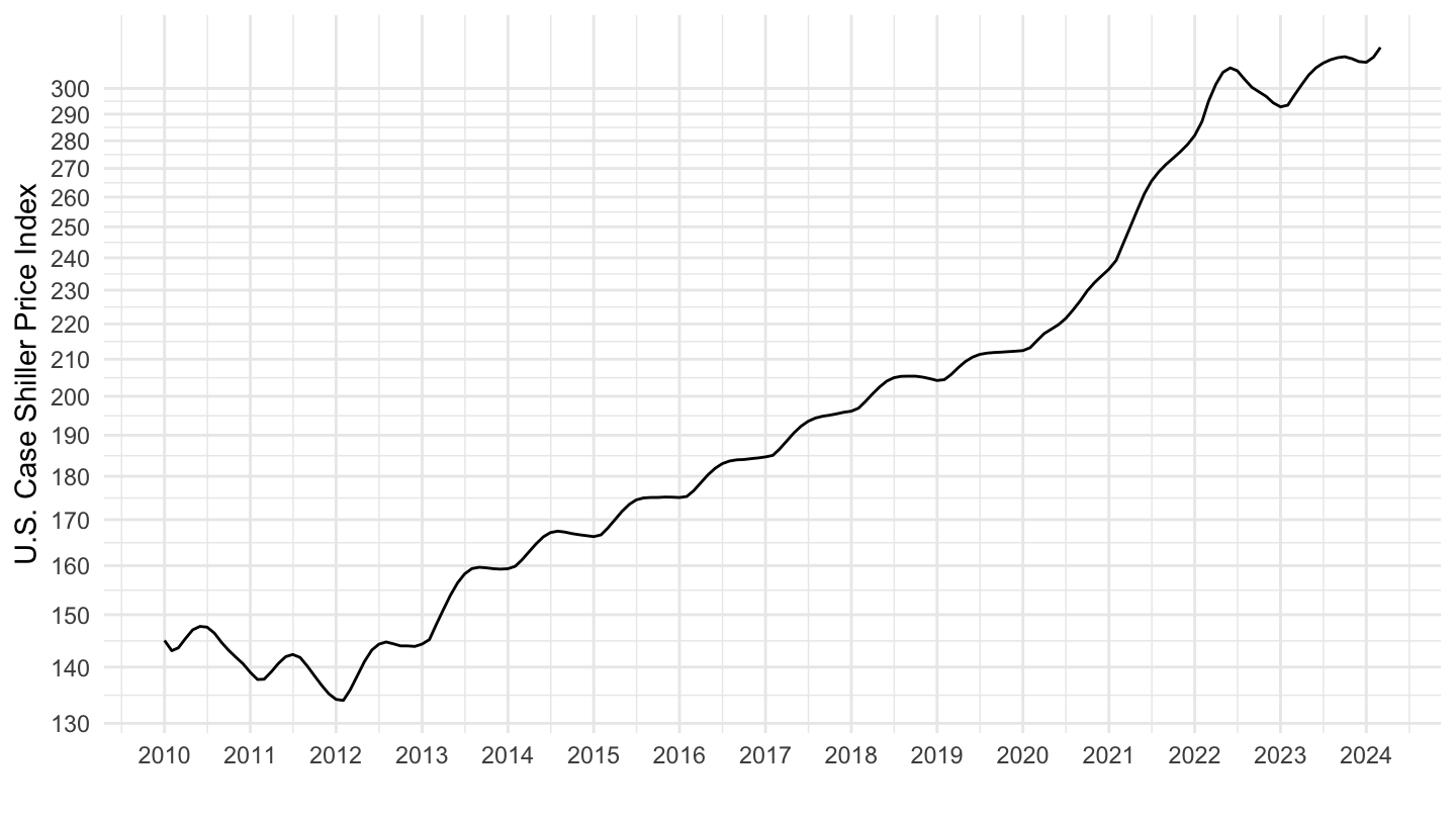
Rents: Rent of Primary residence
U.S.
Normal scale
Code
cpi %>%
  filter(variable %in% c("CUUR0000SEHA", "CPIAUCSL", "CUSR0000SAH1", "CUUR0000SA0L2")) %>%
  left_join(variable, by = "variable") %>%
  filter(year(date) >= 1947) %>%
  ggplot + geom_line(aes(x = date, y = value, color = Variable)) +
  ylab("Types of CPI") + xlab("") +
  theme_minimal() +
  scale_x_date(breaks = seq(1700, 2100, 10) %>% paste0("-01-01") %>% as.Date,
               labels = date_format("%Y")) +
  theme(legend.position = c(0.4, 0.90),
        legend.title = element_blank(),
        legend.key.size = unit(0.9, 'lines')) +
  scale_y_continuous(breaks = seq(0, 350, 50))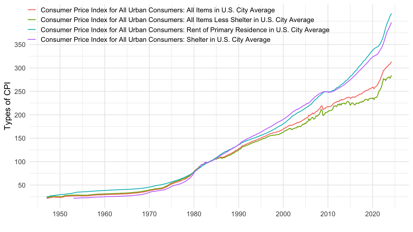
Log scale
(ref:us-cpi-rents-log) Rents: Rent of Primary residence
Code
cpi %>%
  filter(variable %in% c("CUUR0000SEHA", "CPIAUCSL", "CUSR0000SAH1", "CUUR0000SA0L2")) %>%
  left_join(variable, by = "variable") %>%
  filter(year(date) >= 1947) %>%
  ggplot + geom_line(aes(x = date, y = value, color = Variable)) +
  ylab("Types of CPI") + xlab("") +
  theme_minimal() +
  scale_x_date(breaks = seq(1700, 2100, 10) %>% paste0("-01-01") %>% as.Date,
               labels = date_format("%Y")) +
  theme(legend.position = c(0.4, 0.90),
        legend.title = element_blank(),
        legend.key.size = unit(0.9, 'lines')) +
  scale_y_log10(breaks = seq(0, 350, 50))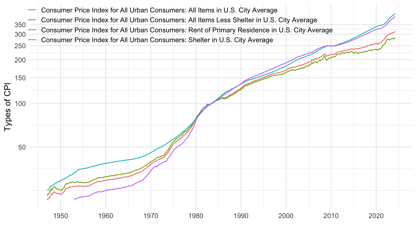
CBSA
Boston, Chicago, New York, Philadelphia
(ref:A101-A102-A103-A207) Boston, Chicago, New York, Philadelphia
Code
cpi %>%
  filter(variable %in% c("CUURA101SEHA", "CUURA102SEHA", "CUURA103SEHA", "CUURA207SEHA")) %>%
  left_join(variable, by = "variable") %>%
  filter(year(date) >= 1978) %>%
  mutate(Variable = gsub("Consumer Price Index for All Urban Consumers: Rent of Primary Residence in ", "", Variable)) %>%
  ggplot + geom_line(aes(x = date, y = value, color = Variable)) +
  ylab("CPI - All Urban Consumers: Rent of Primary Residence") + xlab("") +
  theme_minimal() +
  scale_x_date(breaks = seq(1700, 2100, 5) %>% paste0("-01-01") %>% as.Date,
               labels = date_format("%Y")) +
  theme(legend.position = c(0.3, 0.90),
        legend.title = element_blank(),
        legend.key.size = unit(0.9, 'lines')) +
  scale_y_log10(breaks = seq(0, 350, 50))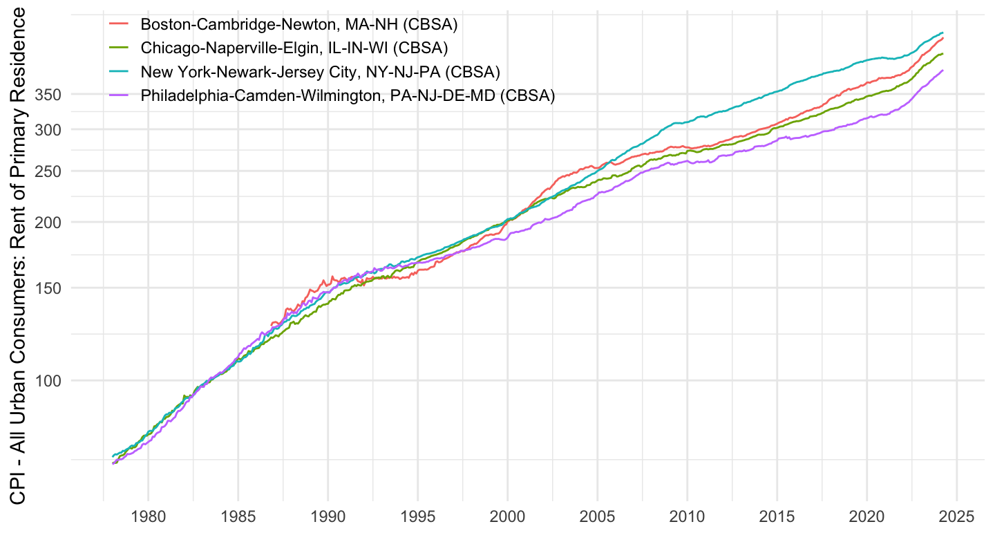
Detroit, Houston, San Francisco, Seattle
(ref:A208-A318-A422-A423) Detroit, Houston, San Francisco, Seattle
Code
cpi %>%
  filter(variable %in% c("CUURA208SEHA", "CUURA318SEHA", "CUURA422SEHA", "CUURA423SEHA")) %>%
  left_join(variable, by = "variable") %>%
  filter(year(date) >= 1978) %>%
  mutate(Variable = gsub("Consumer Price Index for All Urban Consumers: Rent of Primary Residence in ", "", Variable)) %>%
  ggplot + geom_line(aes(x = date, y = value, color = Variable)) +
  ylab("CPI - All Urban Consumers: Rent of Primary Residence") + xlab("") +
  theme_minimal() +
  scale_x_date(breaks = seq(1700, 2100, 5) %>% paste0("-01-01") %>% as.Date,
               labels = date_format("%Y")) +
  theme(legend.position = c(0.3, 0.90),
        legend.title = element_blank(),
        legend.key.size = unit(0.9, 'lines')) +
  scale_y_log10(breaks = seq(0, 350, 50))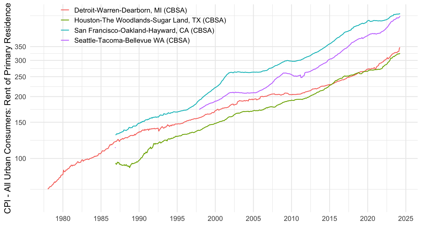
San Francisco
Code
cpi %>%
  filter(variable %in% c("CUURA422SEHA", "CUURA422SEHC", "CUURA422SEHC01", "CUURA422SASL2RS")) %>%
  left_join(variable, by = "variable") %>%
  filter(year(date) >= 1987) %>%
  mutate(Variable = gsub("Consumer Price Index for All Urban Consumers: ", "", Variable),
         Variable = gsub(" in San Francisco-Oakland-Hayward, CA \\(CBSA\\)", "", Variable)) %>%
  ggplot + geom_line(aes(x = date, y = value, color = Variable)) +
  ylab("CPI - All Urban Consumers: Rent of Primary Residence") + xlab("") +
  theme_minimal() +
  scale_x_date(breaks = seq(1700, 2100, 5) %>% paste0("-01-01") %>% as.Date,
               labels = date_format("%Y")) +
  theme(legend.position = c(0.3, 0.90),
        legend.title = element_blank(),
        legend.key.size = unit(0.9, 'lines')) +
  scale_y_log10(breaks = c(seq(0, 500, 50), 450, 550))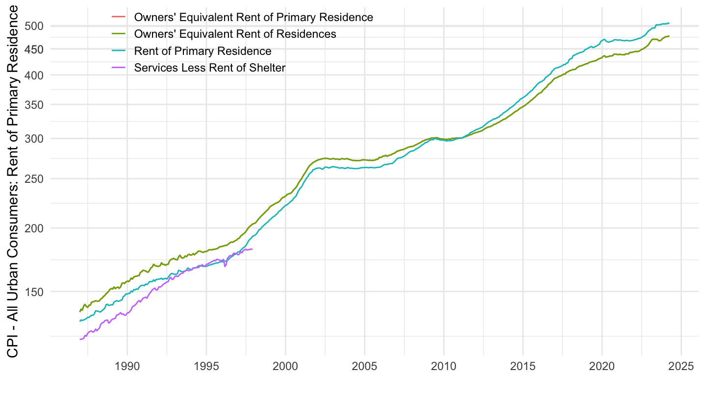
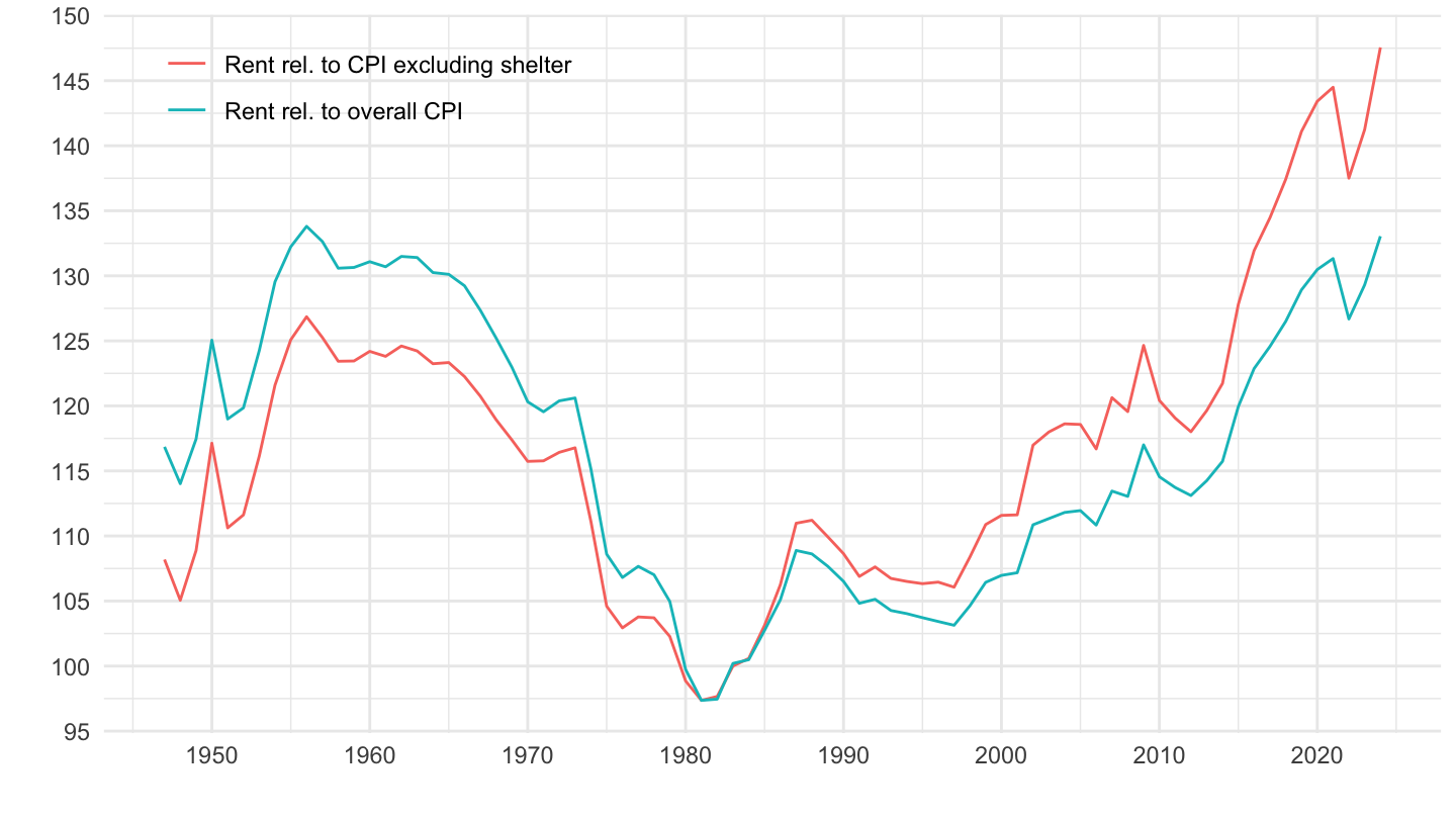
Relative Rent Price
(ref:us-relative-rent-price) Relative Rent Price
Code
cpi %>%
  filter(variable %in% c("CUUR0000SEHA", "CPIAUCSL", "CUUR0000SA0L2")) %>%
  filter(year(date) >= 1947, month(date) == 1) %>%
  spread(variable, value) %>%
  mutate(rent_real = 100*CUUR0000SEHA / CPIAUCSL,
         rent_real_less_shelter = 100*CUUR0000SEHA / CUUR0000SA0L2) %>%
  select(-CUUR0000SEHA, -CPIAUCSL, -CUUR0000SA0L2) %>%
  gather(variable, value, -date) %>%
  mutate(variable_desc = case_when(variable == "rent_real" ~ "Rent rel. to overall CPI",
                                   variable == "rent_real_less_shelter" ~ "Rent rel. to CPI excluding shelter",
                                   variable == "UNRATE" ~ "Unemployment Rate")) %>%
  ggplot + geom_line(aes(x = date, y = value, color = variable_desc)) +
  ylab("") + xlab("") +
  theme_minimal() +
  scale_x_date(breaks = seq(1700, 2100, 10) %>% paste0("-01-01") %>% as.Date,
               labels = date_format("%Y")) +
  theme(legend.position = c(0.2, 0.90),
        legend.title = element_blank()) +
  scale_y_continuous(breaks = seq(0, 350, 5))