Indices des prix à la consommation - Base 1990

Données - INSEE

Auteur

François Geerolf

Info

Last observation: 1998-12

First observation: 1990

Number of observations: 69 239

Last data update: 23 jul 2026, 22:49. Last compile: 24 jul 2026, 06:01

Structure

Données sur l’inflation en France

source	dataset	Title	.html	.rData
insee	ILC-ILAT-ICC	Indices pour la révision d’un bail commercial ou professionnel	2026-07-23	2026-07-23
insee	INDICES_LOYERS	Indices des loyers d'habitation (ILH)	2026-07-23	2026-07-23
insee	IPC-1970-1980	Indice des prix à la consommation - Base 1970, 1980	2026-07-23	2026-07-23
insee	IPC-1990	Indices des prix à la consommation - Base 1990	2026-07-23	2026-07-23
insee	IPC-2015	Indice des prix à la consommation - Base 2015	2026-07-23	2026-07-23
insee	IPC-PM-2015	Prix moyens de vente de détail	2026-07-23	2026-07-23
insee	IPCH-2015	Indices des prix à la consommation harmonisés	2026-07-23	2026-07-23
insee	IPCH-IPC-2015-ensemble	Indices des prix à la consommation harmonisés	2026-07-23	2026-07-23
insee	IPGD-2015	Indice des prix dans la grande distribution	2026-07-23	2026-07-23
insee	IPLA-IPLNA-2015	Indices des prix des logements neufs et Indices Notaires-Insee des prix des logements anciens	2026-07-23	2026-07-23
insee	IPPI-2015	Indices de prix de production et d'importation dans l'industrie	2026-07-23	2026-07-23
insee	IRL	Indice pour la révision d’un loyer d’habitation	2026-07-23	2026-07-23
insee	SERIES_LOYERS	Variation des loyers	2026-07-23	2026-07-23
insee	T_CONSO_EFF_FONCTION	Consommation effective des ménages par fonction	2026-07-23	2025-12-22
insee	bdf2017	Budget de famille 2017	2026-07-23	2023-11-21
insee	echantillon-agglomerations-IPC-2024	Échantillon d’agglomérations enquêtées de l’IPC en 2024	2026-07-23	2026-01-27
insee	echantillon-agglomerations-IPC-2025	Échantillon d’agglomérations enquêtées de l’IPC en 2025	2026-07-23	2026-01-27
insee	liste-varietes-IPC-2024	Liste des variétés pour la mesure de l'IPC en 2024	2026-07-23	2025-04-02
insee	liste-varietes-IPC-2025	Liste des variétés pour la mesure de l'IPC en 2025	2026-07-23	2026-01-27
insee	ponderations-elementaires-IPC-2024	Pondérations élémentaires 2024 intervenant dans le calcul de l’IPC	2026-07-23	2025-04-02
insee	ponderations-elementaires-IPC-2025	Pondérations élémentaires 2025 intervenant dans le calcul de l’IPC	2026-07-23	2026-01-27
insee	table_conso_moyenne_par_categorie_menages	Montants de consommation selon différentes catégories de ménages	2026-07-23	2026-01-27
insee	table_poste_au_sein_sous_classe_ecoicopv2_france_entiere_	Ventilation de chaque sous-classe (niveau 4 de la COICOP v2) en postes et leurs pondérations	2026-07-23	2026-01-27
insee	tranches_unitesurbaines	Poids de chaque tranche d’unités urbaines dans la consommation	2026-07-23	2026-01-27

Data on inflation

source	dataset	Title	.html	.rData
bis	CPI	Consumer Price Index	2026-07-22	2026-07-22
ecb	CES	Consumer Expectations Survey	2026-07-23	2026-07-19
eurostat	nama_10_co3_p3	Final consumption expenditure of households by consumption purpose (COICOP 3 digit)	2026-07-18	2026-07-23
eurostat	prc_hicp_cow	HICP - country weights	2026-07-23	2026-07-23
eurostat	prc_hicp_ctrb	Contributions to euro area annual inflation (in percentage points)	2026-07-23	2026-07-23
eurostat	prc_hicp_inw	HICP - item weights	2026-07-23	2026-07-23
eurostat	prc_hicp_manr	HICP (2015 = 100) - monthly data (annual rate of change)	2026-07-23	2026-07-23
eurostat	prc_hicp_midx	HICP (2015 = 100) - monthly data (index)	2026-07-23	2026-07-23
eurostat	prc_hicp_mmor	HICP (2015 = 100) - monthly data (monthly rate of change)	2026-07-23	2026-07-23
eurostat	prc_ppp_ind	Purchasing power parities (PPPs), price level indices and real expenditures for ESA 2010 aggregates	2026-07-22	2026-07-23
eurostat	sts_inpp_m	Producer prices in industry, total - monthly data	2026-07-21	2026-07-23
eurostat	sts_inppd_m	Producer prices in industry, domestic market - monthly data	2026-07-21	2026-07-23
eurostat	sts_inppnd_m	Producer prices in industry, non domestic market - monthly data	2026-07-21	2026-07-23
fred	cpi	Consumer Price Index	2026-07-22	2026-07-22
fred	inflation	Inflation	2026-07-22	2026-07-22
imf	CPI	Consumer Price Index (CPI) 2026 February - CPI_2026_FEB_VINTAGE	2026-07-22	2026-04-13
oecd	MEI_PRICES_PPI	Producer Prices - MEI_PRICES_PPI	2026-07-23	2024-04-15
oecd	PPP2017	2017 PPP Benchmark results	2024-04-16	2023-07-25
oecd	PRICES_CPI	Consumer price indices (CPIs)	2024-04-16	2024-04-15
wdi	FP.CPI.TOTL.ZG	Inflation, consumer prices (annual %)	2026-07-22	2026-07-22
wdi	NY.GDP.DEFL.KD.ZG	Inflation, GDP deflator (annual %)	2026-07-22	2026-07-22

LAST_COMPILE

LAST_COMPILE
2026-07-24

Last TIME_PERIOD

Code

`IPC-1990` %>%
  group_by(TIME_PERIOD) %>%
  summarise(Nobs = n()) %>%
  arrange(desc(TIME_PERIOD)) %>%
  head(1) %>%
  print_table_conditional()

TIME_PERIOD	Nobs
1998-12	587

Pondérations d’indice

1992, 1994, 1996, 1998

Code

`IPC-1990` %>%
  filter(NATURE == "POND",
         TIME_PERIOD %in% c("1998", "1996", "1994", "1992", "1990"),
         MENAGES_IPC == "POPULATION-TOTALE") %>%
  select_if(function(col) length(unique(col)) > 1) %>%
  select(-IDBANK, -TITLE_FR, -TITLE_EN, -OBS_STATUS, -OBS_TYPE) %>%
  
  
  spread(TIME_PERIOD, OBS_VALUE) %>%
  print_table_conditional

Tabac

Code

`IPC-1990` %>%
  filter(INDICATEUR == "IPC",
         MENAGES_IPC == "POPULATION-TOTALE",
         COICOP_1990 %in% c("14"),
         NATURE == "POND") %>%
  year_to_date %>%
  mutate(OBS_VALUE = OBS_VALUE/10000) %>%
  ggplot() + ylab("Poids du tabac dans l'indice des prix") + xlab("") + theme_minimal() +
  geom_line(aes(x = date, y = OBS_VALUE)) +
  scale_color_manual(values = viridis(3)[1:2]) +
  scale_x_date(breaks = seq(1920, 2025, 1) %>% paste0("-01-01") %>% as.Date,
               labels = date_format("%Y")) +
  scale_y_continuous(breaks = 0.01*seq(0, 10, 0.1),
                     labels = percent_format(accuracy = .1))

Santé

Code

`IPC-1990` %>%
  filter(INDICATEUR == "IPC",
         MENAGES_IPC == "POPULATION-TOTALE",
         COICOP_1990 %in% c("5"),
         NATURE == "POND") %>%
  year_to_date %>%
  mutate(OBS_VALUE = OBS_VALUE/10000) %>%
  ggplot() + ylab("Poids de la santé dans l'indice des prix") + xlab("") + theme_minimal() +
  geom_line(aes(x = date, y = OBS_VALUE)) +
  scale_color_manual(values = viridis(3)[1:2]) +
  scale_x_date(breaks = seq(1920, 2025, 1) %>% paste0("-01-01") %>% as.Date,
               labels = date_format("%Y")) +
  scale_y_continuous(breaks = 0.01*seq(0, 10, 0.1),
                     labels = percent_format(accuracy = .1))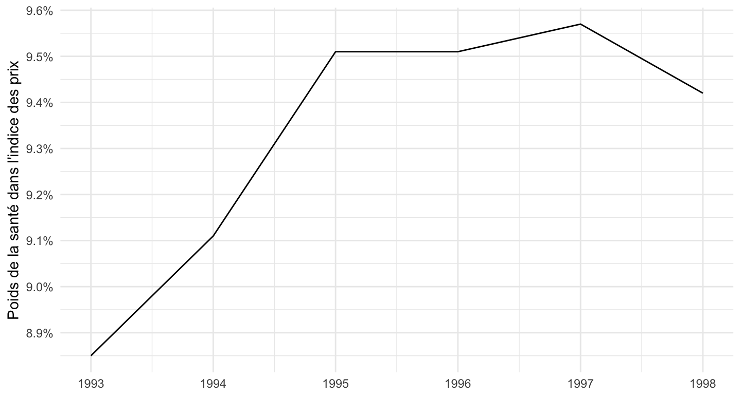

2-digit

Boissons Alcoolisées, Logement, Restaurants et hôtels

Code

`IPC-1990` %>%
  filter(COICOP_1990 %in% c("0", "2", "11", "4"),
         REF_AREA == "FE",
         NATURE == "INDICE",
         FREQ == "M") %>%
  month_to_date %>%
  
  group_by(COICOP_1990) %>%
  arrange(date) %>%
  mutate(OBS_VALUE = 100*OBS_VALUE/OBS_VALUE[1]) %>%
  ggplot() + ylab("Indice des prix") + xlab("") + theme_minimal() +
  geom_line(aes(x = date, y = OBS_VALUE, color = Coicop_1990)) +
  scale_color_manual(values = viridis(5)[1:4]) +
  scale_x_date(breaks = seq(1920, 2025, 1) %>% paste0("-01-01") %>% as.Date,
               labels = date_format("%Y")) +
  theme(legend.position = c(0.3, 0.85),
        legend.title = element_blank()) +
  scale_y_log10(breaks = seq(100, 200, 1),
                     labels = dollar_format(accuracy = 1, prefix = ""))

Transports, Enseignement, B&S Divers

Code

`IPC-1990` %>%
  filter(COICOP_1990 %in% c("00", "1", "7", "12"),
         REF_AREA == "FE",
         NATURE == "INDICE",
         FREQ == "M") %>%
  month_to_date %>%
  
  group_by(COICOP_1990) %>%
  arrange(date) %>%
  mutate(OBS_VALUE = 100*OBS_VALUE/OBS_VALUE[1]) %>%
  ggplot() + ylab("Indice des prix") + xlab("") + theme_minimal() +
  geom_line(aes(x = date, y = OBS_VALUE, color = Coicop_1990)) +
  scale_color_manual(values = viridis(5)[1:4]) +
  scale_x_date(breaks = seq(1920, 2025, 2) %>% paste0("-01-01") %>% as.Date,
               labels = date_format("%Y")) +
  theme(legend.position = c(0.3, 0.85),
        legend.title = element_blank()) +
  scale_y_log10(breaks = seq(100, 300, 1),
                     labels = dollar_format(accuracy = 1, prefix = ""))

Alimentation, Habillement, Meubles

Code

`IPC-1990` %>%
  filter(COICOP_1990 %in% c("00", "5", "1", "3"),
         REF_AREA == "FE",
         NATURE == "INDICE",
         FREQ == "M") %>%
  month_to_date %>%
  
  group_by(COICOP_1990) %>%
  arrange(date) %>%
  mutate(OBS_VALUE = 100*OBS_VALUE/OBS_VALUE[1]) %>%
  ggplot() + ylab("Indice des prix") + xlab("") + theme_minimal() +
  geom_line(aes(x = date, y = OBS_VALUE, color = Coicop_1990)) +
  scale_color_manual(values = viridis(5)[1:4]) +
  scale_x_date(breaks = seq(1920, 2025, 1) %>% paste0("-01-01") %>% as.Date,
               labels = date_format("%Y")) +
  theme(legend.position = c(0.3, 0.85),
        legend.title = element_blank()) +
  scale_y_log10(breaks = seq(100, 300, 1),
                     labels = dollar_format(accuracy = 1, prefix = ""))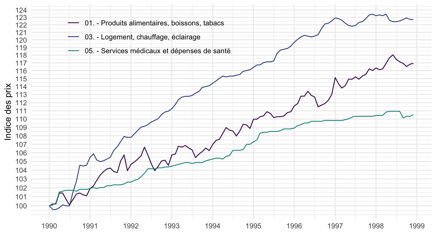

Santé, Communications, Loisirs

Code

`IPC-1990` %>%
  filter(COICOP_1990 %in% c("00", "6", "9", "8"),
         REF_AREA == "FE",
         NATURE == "INDICE",
         FREQ == "M") %>%
  month_to_date %>%
  
  group_by(COICOP_1990) %>%
  arrange(date) %>%
  mutate(OBS_VALUE = 100*OBS_VALUE/OBS_VALUE[1]) %>%
  ggplot() + ylab("Indice des prix") + xlab("") + theme_minimal() +
  geom_line(aes(x = date, y = OBS_VALUE, color = Coicop_1990)) +
  scale_color_manual(values = viridis(5)[1:4]) +
  scale_x_date(breaks = seq(1920, 2025, 2) %>% paste0("-01-01") %>% as.Date,
               labels = date_format("%Y")) +
  theme(legend.position = c(0.2, 0.85),
        legend.title = element_blank()) +
  scale_y_log10(breaks = seq(10, 300, 10),
                     labels = dollar_format(accuracy = 1, prefix = ""))