
Last observation: 2025 (N = 18498)
First observation: 1996 (N = 4773)
Last data update: 09 sept. 2026, 07:47
Last compile: 09 oct. 2026, 23:03
prc_hicp_inw |>

  filter(geo == "FR",
         substr(coicop, 1, 2) == "CP" ,
         coicop != "CP00",
         time %in% c("2017", "2023")) |>
  select(-geo) |>
  spread(time, values) |>
print_table_conditional()`table1-2digit` <- prc_hicp_inw |>
filter(geo == "FR",
nchar(coicop) == 4,
substr(coicop, 1, 2) == "CP" ,
coicop != "CP00",
time %in% c("2017", "2023")) |>
select(-geo) |>
spread(time, values)
`table1-2digit` |>
print_table_conditional()| freq | Freq | coicop | Coicop | Geo | 2017 | 2023 |
|---|---|---|---|---|---|---|
| A | Annual | CP01 | Food and non-alcoholic beverages | France | 160.04 | 161.90 |
| A | Annual | CP02 | Alcoholic beverages, tobacco and narcotics | France | 42.41 | 40.95 |
| A | Annual | CP03 | Clothing and footwear | France | 49.60 | 40.13 |
| A | Annual | CP04 | Housing, water, electricity, gas and other fuels | France | 157.96 | 164.05 |
| A | Annual | CP05 | Furnishings, household equipment and routine household maintenance | France | 58.53 | 55.61 |
| A | Annual | CP06 | Health | France | 44.59 | 42.25 |
| A | Annual | CP07 | Transport | France | 159.15 | 164.75 |
| A | Annual | CP08 | Communications | France | 31.85 | 27.58 |
| A | Annual | CP09 | Recreation and culture | France | 89.23 | 80.92 |
| A | Annual | CP10 | Education | France | 3.81 | 4.80 |
| A | Annual | CP11 | Restaurants and hotels | France | 83.10 | 99.18 |
| A | Annual | CP12 | Miscellaneous goods and services | France | 119.73 | 117.87 |
`table1-2digit` |>
  gt::gt() |>
gt::gtsave(filename = "prc_hicp_inw_files/figure-html/table1-2digit-1.png")`table1-3digit` <- prc_hicp_inw |>
filter(geo == "FR",
nchar(coicop) == 5 | coicop == "CP082_083",
substr(coicop, 1, 2) == "CP" ,
coicop != "CP00",
time %in% c("2017", "2023")) |>
select(-geo) |>
spread(time, values)
`table1-3digit` |>
print_table_conditional()`table1-3digit` |>
gt::gt() |>
gt::gtsave(filename = "prc_hicp_inw_files/figure-html/table1-3digit-1.png")prc_hicp_inw |>
filter(coicop %in% c(paste0("CP0", 1:9), paste0(paste0("CP1", 1:2))),
geo %in% c("FR")) |>
year_to_date() |>
ggplot() + theme_minimal() + ylab("") + xlab("") +
geom_area(aes(x = date, y = values/1000, fill = paste(coicop, Coicop)),
position = "stack") +
#scale_color_manual(values = viridis(4)[1:3]) +
scale_x_date(breaks = seq(1920, 2100, 2) |> paste0("-01-01") |> as.Date(),
labels = date_format("%Y")) +
theme(legend.position = c(0.38, 0.5),
legend.title = element_blank(),
legend.direction = "vertical",
legend.key.height = unit(0.5, "lines"), # 🔽 Reduce vertical spacing
legend.text = element_text(size = 9)) +
scale_y_continuous(breaks = 0.01*seq(0, 100, 5),
labels = percent_format(a = 1),
limits = c(0, 1))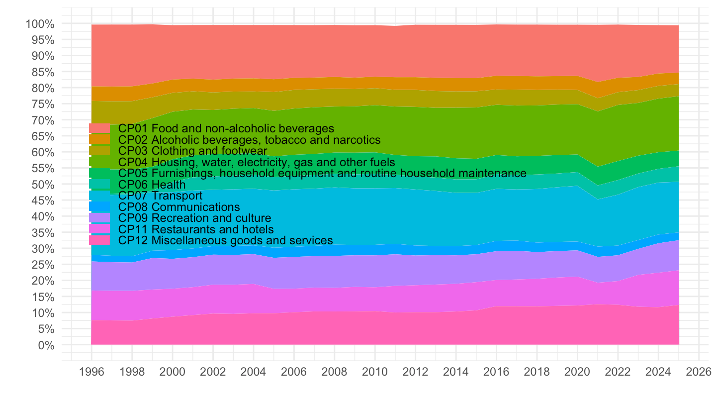
coicop <- read_parquet("coicop_fr.parquet")
prc_hicp_inw |>
  filter(coicop %in% c(paste0("CP0", 1:9), paste0(paste0("CP1", 1:2))),
         geo %in% c("FR")) |>
  year_to_date() |>

  ggplot() + theme_minimal() + ylab("") + xlab("") +
  geom_area(aes(x = date, y = values/1000, fill = paste(coicop, Coicop)),
            position = "stack") +
  #scale_color_manual(values = viridis(4)[1:3]) +
  scale_x_date(breaks = seq(1920, 2100, 2) |> paste0("-01-01") |> as.Date(),
               labels = date_format("%Y")) +
  theme(legend.position = c(0.38, 0.5),
        legend.title = element_blank(),
        legend.direction = "vertical",
        legend.key.height = unit(0.5, "lines"),   # 🔽 Reduce vertical spacing
        legend.text = element_text(size = 9)) +
  scale_y_continuous(breaks = 0.01*seq(0, 100, 5),
               labels = percent_format(a = 1),
               limits = c(0, 1))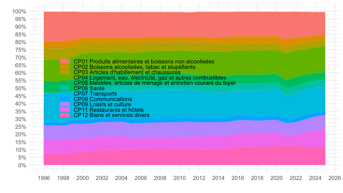
coicop <- read_parquet("coicop.parquet")
prc_hicp_inw |>
  filter(coicop %in% c("GD", "SERV"),
         geo %in% c("FR")) |>
  year_to_date() |>

  ggplot() + theme_minimal() + ylab("") + xlab("") +
  geom_area(aes(x = date, y = values/1000, fill = paste(coicop, Coicop)),
            position = "stack") +
  #scale_color_manual(values = viridis(4)[1:3]) +
  scale_x_date(breaks = seq(1920, 2100, 2) |> paste0("-01-01") |> as.Date(),
               labels = date_format("%Y")) +
  theme(legend.position = c(0.5, 0.9),
        legend.title = element_blank(),
        legend.direction = "vertical",
        legend.key.height = unit(0.5, "lines"),   # 🔽 Reduce vertical spacing
        legend.text = element_text(size = 9)) +
  scale_y_continuous(breaks = 0.01*seq(0, 100, 5),
               labels = percent_format(a = 1),
               limits = c(0, 1))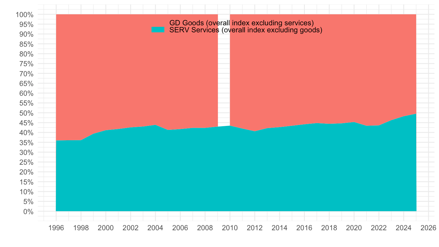
IGD_NNRG_ND: 0441, 0611, 0612_3, 0431, 0561, 0933, 0935, 0952, 0953_4, 1212_3
IGD_NNRG_SD: 0311, 0312, 0313, 032, 052, 054, 055, 0721, 0914, 0931, 0932, 0951, 1232
IGD_NNRG_D: 0511, 0512, 0531_2, 0711, 0712_34, 0911, 0912, 0913, 0921_2, 1231
SERVICES: Services related to communication (includes phone plans)
SERV_COM: Services related to communication 081, 08x
SERV_REC: Services related to housing 041, 0432, 0442, 0443, 0444, 0513, 0533, 0562, 1252
SERV_TRA: prix du train, de la SNCF
prc_hicp_inw |>
  filter(coicop %in% c("IGD_NNRG_D", "IGD_NNRG_ND", "IGD_NNRG_SD", "SERV", "NRG", "FOOD"),
         geo %in% c("FR")) |>
  year_to_date() |>

  ggplot() + theme_minimal() + ylab("") + xlab("") +
  geom_area(aes(x = date, y = values/1000, fill = paste(coicop, Coicop)),
            position = "stack") +
  #scale_color_manual(values = viridis(4)[1:3]) +
  scale_x_date(breaks = seq(1920, 2100, 2) |> paste0("-01-01") |> as.Date(),
               labels = date_format("%Y")) +
  theme(legend.position = "bottom",
        legend.title = element_blank(),
        legend.direction = "vertical",
        legend.key.height = unit(0.5, "lines"),   # 🔽 Reduce vertical spacing
        legend.text = element_text(size = 9)) +
  scale_y_continuous(breaks = 0.01*seq(0, 100, 5),
               labels = percent_format(a = 1),
               limits = c(0, 1))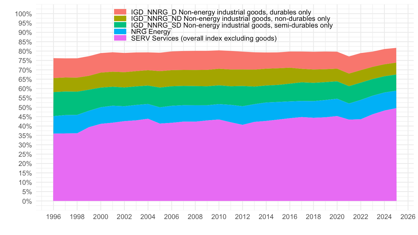
prc_hicp_inw |>
  filter(coicop %in% c("IGD_NNRG_D", "IGD_NNRG_ND", "IGD_NNRG_SD", "NRG"),
         geo %in% c("FR")) |>
  year_to_date() |>

  ggplot() + theme_minimal() + ylab("") + xlab("") +
  geom_area(aes(x = date, y = values/1000, fill = paste(coicop, Coicop)),
            position = "stack") +
  #scale_color_manual(values = viridis(4)[1:3]) +
  scale_x_date(breaks = seq(1920, 2100, 2) |> paste0("-01-01") |> as.Date(),
               labels = date_format("%Y")) +
  theme(legend.position = c(0.5, 0.9),
        legend.title = element_blank(),
        legend.direction = "vertical",
        legend.key.height = unit(0.5, "lines"),   # 🔽 Reduce vertical spacing
        legend.text = element_text(size = 9)) +
  scale_y_continuous(breaks = 0.01*seq(0, 100, 5),
               labels = percent_format(a = 1),
               limits = c(0, 1))
prc_hicp_inw |>
  filter(coicop %in% c("CP0820", "CP0830", "CP08", "CP091", "CP053"),
         geo %in% c("FR")) |>
  year_to_date() |>

  ggplot() + theme_minimal() + ylab("") + xlab("") +
  geom_line(aes(x = date, y = values/1000, color = paste(coicop, Coicop))) +
  #scale_color_manual(values = viridis(4)[1:3]) +
  scale_x_date(breaks = seq(1920, 2100, 2) |> paste0("-01-01") |> as.Date(),
               labels = date_format("%Y")) +
  theme(legend.position = c(0.35, 0.8),
        legend.title = element_blank()) +
  scale_y_continuous(breaks = seq(0, 1, 0.005),
               labels = percent_format(a = .1))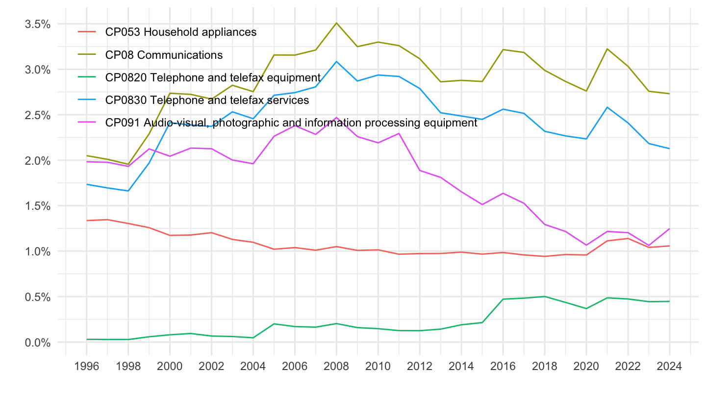
prc_hicp_inw |>
  filter(coicop %in% c("CP0820", "CP0830", "CP08", "CP091", "CP053", "CP071"),
         geo %in% c("FR")) |>
  year_to_date() |>

  ggplot() + theme_minimal() + ylab("") + xlab("") +
  geom_line(aes(x = date, y = values/1000, color = paste(coicop, Coicop))) +
  #scale_color_manual(values = viridis(4)[1:3]) +
  scale_x_date(breaks = seq(1920, 2100, 2) |> paste0("-01-01") |> as.Date(),
               labels = date_format("%Y")) +
  theme(legend.position = c(0.45, 0.8),
        legend.title = element_blank()) +
  scale_y_continuous(breaks = seq(0, 1, 0.005),
               labels = percent_format(a = .1))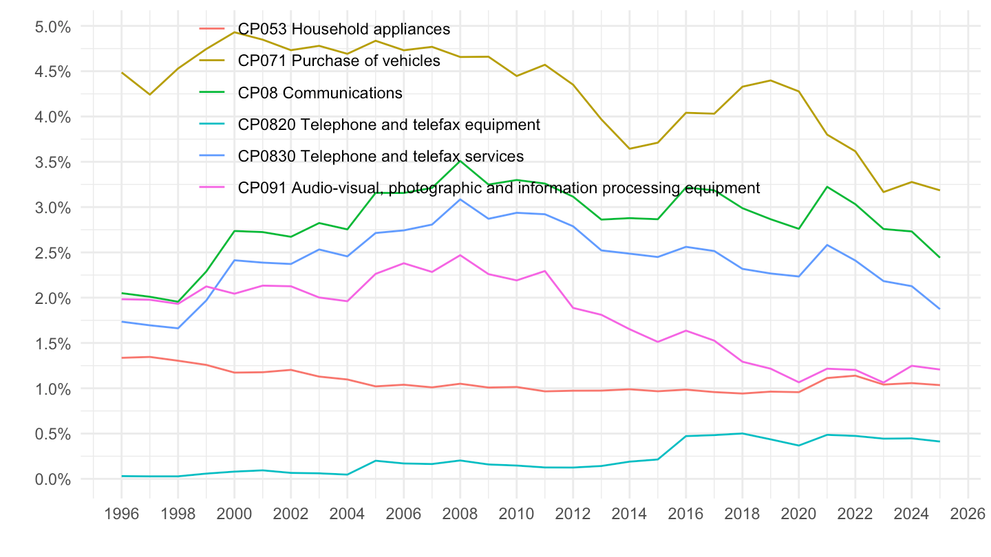
Habillement aussi ! Loyers aussi !
prc_hicp_inw |>
  filter(coicop %in% c("CP0820", "CP0830", "CP091", "CP053", "CP071"),
         geo %in% c("FR")) |>
  year_to_date() |>

  ggplot() + theme_minimal() + ylab("") + xlab("") +
  geom_area(aes(x = date, y = values/1000, fill = paste(coicop, Coicop)),
            position = "stack") +
  #scale_color_manual(values = viridis(4)[1:3]) +
  scale_x_date(breaks = seq(1920, 2100, 2) |> paste0("-01-01") |> as.Date(),
               labels = date_format("%Y")) +
  theme(legend.position = c(0.5, 0.85),
        legend.title = element_blank(),
        legend.direction = "vertical",
        legend.key.height = unit(0.5, "lines"),   # 🔽 Reduce vertical spacing
        legend.text = element_text(size = 9)) +
  scale_y_continuous(breaks = 0.01*seq(0, 100, 1),
               labels = percent_format(a = 1),
               limits = c(0, 0.15))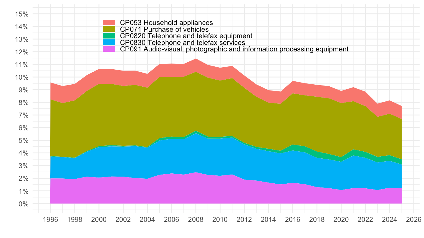
Car il y a aussi les remplacements en réalité…
prc_hicp_inw |>
  filter(coicop %in% c("CP041", "CP03", "CP0820", "CP041", "CP03", "CP0830", "CP091", "CP053", "CP071"),
         geo %in% c("FR")) |>
  year_to_date() |>

  ggplot() + theme_minimal() + ylab("") + xlab("") +
  geom_area(aes(x = date, y = values/1000, fill = paste(coicop, Coicop)),
            position = "stack") +
  #scale_color_manual(values = viridis(4)[1:3]) +
  scale_x_date(breaks = seq(1920, 2100, 2) |> paste0("-01-01") |> as.Date(),
               labels = date_format("%Y")) +
  theme(legend.position = c(0.5, 0.85),
        legend.title = element_blank(),
        legend.direction = "vertical",
        legend.key.height = unit(0.5, "lines"),   # 🔽 Reduce vertical spacing
        legend.text = element_text(size = 9)) +
  scale_y_continuous(breaks = 0.01*seq(0, 100, 1),
               labels = percent_format(a = 1))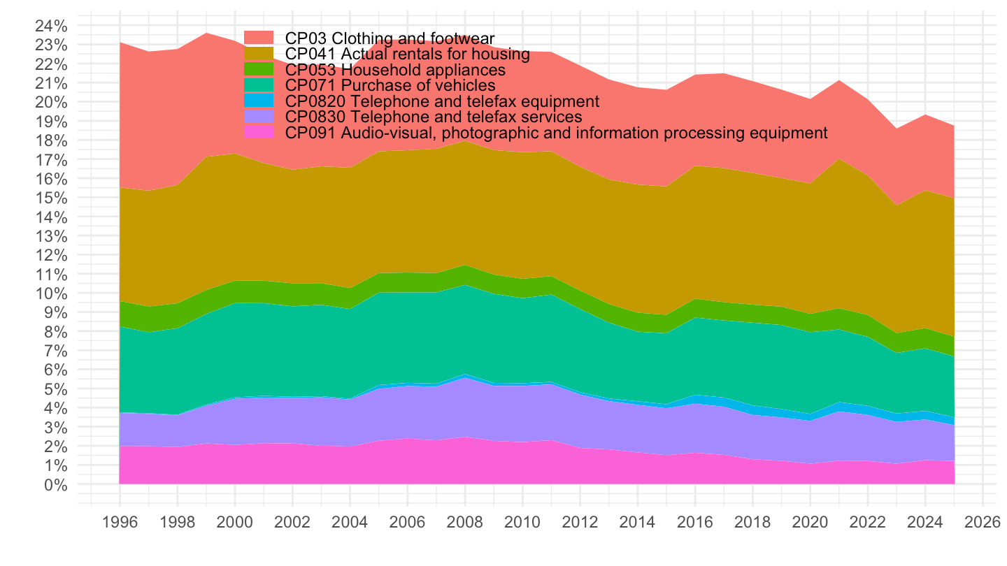
prc_hicp_inw |>
  filter(coicop %in% c("CP01", "CP04", "CP07"),
         geo %in% c("FR")) |>
  year_to_date() |>

  ggplot() + theme_minimal() + ylab("") + xlab("") +
  geom_line(aes(x = date, y = values/1000, color = Coicop)) +
  #scale_color_manual(values = viridis(4)[1:3]) +
  scale_x_date(breaks = seq(1920, 2100, 2) |> paste0("-01-01") |> as.Date(),
               labels = date_format("%Y")) +
  theme(legend.position = c(0.7, 0.9),
        legend.title = element_blank()) +
  scale_y_continuous(breaks = seq(0, 1, 0.01),
               labels = percent_format(a = 1))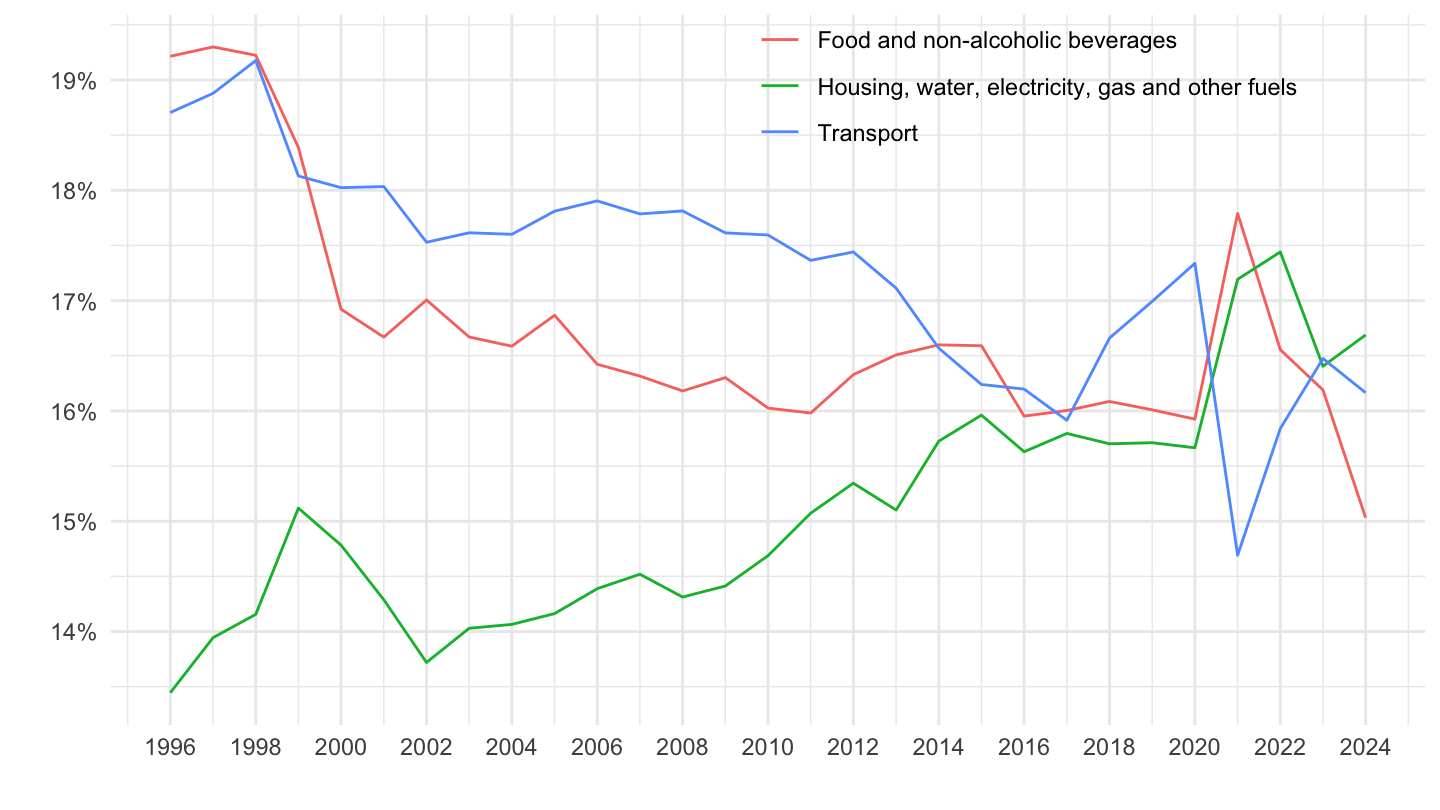
prc_hicp_inw |>
  filter(coicop %in% c("CP05", "CP09", "CP11", "CP12"),
         geo %in% c("FR")) |>
  year_to_date() |>

  ggplot() + theme_minimal() + ylab("") + xlab("") +
  geom_line(aes(x = date, y = values/1000, color = Coicop)) +
  #scale_color_manual(values = viridis(5)[1:4]) +
  scale_x_date(breaks = seq(1920, 2100, 2) |> paste0("-01-01") |> as.Date(),
               labels = date_format("%Y")) +
  theme(legend.position = c(0.4, 0.85),
        legend.title = element_blank()) +
  scale_y_continuous(breaks = seq(0, 1, 0.01),
               labels = percent_format(a = 1))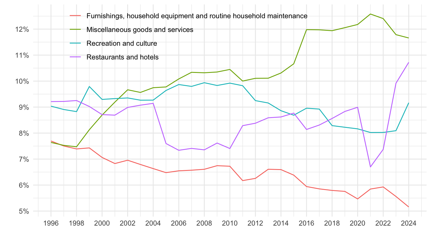
prc_hicp_inw |>
  filter(coicop %in% c("CP02", "CP03", "CP06", "CP08"),
         geo %in% c("FR")) |>
  year_to_date() |>

  ggplot() + theme_minimal() + ylab("") + xlab("") +
  geom_line(aes(x = date, y = values/1000, color = Coicop)) +
  #scale_color_manual(values = viridis(5)[1:4]) +
  scale_x_date(breaks = seq(1920, 2100, 2) |> paste0("-01-01") |> as.Date(),
               labels = date_format("%Y")) +
  theme(legend.position = c(0.73, 0.85),
        legend.title = element_blank()) +
  scale_y_continuous(breaks = seq(0, 1, 0.01),
               labels = percent_format(a = 1))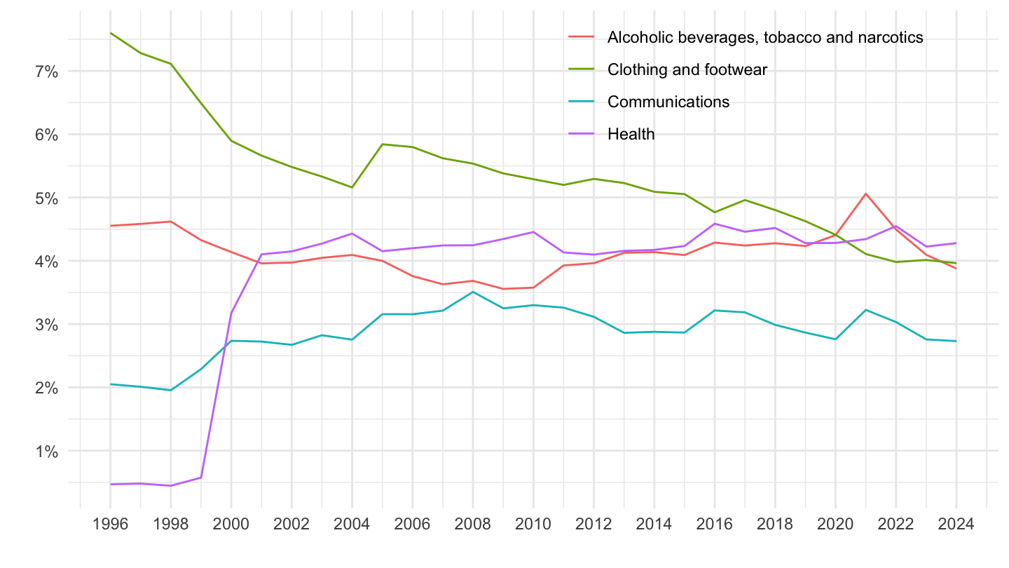
prc_hicp_inw |>
  filter(time %in% c("2022"),
         coicop %in% c("AP_NRG", "NRG", "CP045", "CP0722")) |>

  mutate(values = round(values/10, 1)) |>
  select(Geo, coicop, values) |>
  spread(coicop, values) |>
  transmute(Geo,
            `Energy, Non Adm` = NRG - AP_NRG,
            `Electricity, gas and other fuels` = CP045,
            `Fuels and lubricants` = CP0722,
            `Energy, Adm` = AP_NRG,
            Energy = NRG) |>
  arrange(-`Energy, Non Adm`) |>
  mutate(Flag = gsub(" ", "-", str_to_lower(Geo)),
         Flag = paste0('<img src="../../icon/flag/vsmall/', Flag, '.png" alt="Flag">')) |>
  select(Flag, everything()) %>%
{if (is_html_output()) datatable(., filter = 'top', rownames = F, escape = F) else .}prc_hicp_inw |>
filter(time == "2020",
geo %in% c("FR", "DE", "IT")) |>
select(coicop, Coicop, Geo, values) |>
mutate(values = values/10) |>
spread(Geo, values) %>%
{if (is_html_output()) datatable(., filter = 'top', rownames = F) else .}prc_hicp_inw |>
filter(time == "2010",
geo %in% c("FR", "DE", "IT")) |>
select(coicop, Coicop, Geo, values) |>
mutate(values = values/10) |>
spread(Geo, values) %>%
{if (is_html_output()) datatable(., filter = 'top', rownames = F) else .}prc_hicp_inw |>
filter(time == "2000",
geo %in% c("FR", "DE", "IT")) |>
select(coicop, Coicop, Geo, values) |>
spread(Geo, values) %>%
{if (is_html_output()) datatable(., filter = 'top', rownames = F) else .}prc_hicp_inw |>
filter(time %in% c("2022", "2023", "2024"),
geo %in% c("FR"),
nchar(coicop) %in% c(4, 5) | coicop %in% c("CP0820", "CP0830")) |>
mutate(values = values/10) |>
select(coicop, Coicop, time, values) |>
spread(time, values) %>%
{if (is_html_output()) datatable(., filter = 'top', rownames = F) else .}prc_hicp_inw |>
filter(time %in% c("2000", "2010", "2020"),
geo %in% c("FR"),
nchar(coicop) == 4) |>
select(coicop, Coicop, time, values) |>
spread(time, values) %>%
{if (is_html_output()) datatable(., filter = 'top', rownames = F) else .}prc_hicp_inw |>
filter(time %in% c("2000", "2010", "2020"),
geo %in% c("FR"),
nchar(coicop) %in% c(4, 5)) |>
select(coicop, Coicop, time, values) |>
spread(time, values) %>%
{if (is_html_output()) datatable(., filter = 'top', rownames = F) else .}prc_hicp_inw |>
filter(time %in% c("2000", "2010", "2020"),
geo %in% c("FR")) |>
select(coicop, Coicop, time, values) |>
spread(time, values) %>%
{if (is_html_output()) datatable(., filter = 'top', rownames = F) else .}prc_hicp_inw |>
filter(time %in% c("2000", "2010", "2020"),
geo %in% c("DE"),
nchar(coicop) == 4) |>
select(coicop, Coicop, time, values) |>
spread(time, values) %>%
{if (is_html_output()) datatable(., filter = 'top', rownames = F) else .}prc_hicp_inw |>
filter(time %in% c("2000", "2010", "2020"),
geo %in% c("DE"),
nchar(coicop) %in% c(4,5)) |>
select(coicop, Coicop, time, values) |>
spread(time, values) %>%
{if (is_html_output()) datatable(., filter = 'top', rownames = F) else .}prc_hicp_inw |>
filter(time %in% c("2000", "2010", "2020"),
geo %in% c("DE")) |>
select(coicop, Coicop, time, values) |>
spread(time, values) %>%
{if (is_html_output()) datatable(., filter = 'top', rownames = F) else .}prc_hicp_inw |>
filter(time %in% c("2000", "2010", "2020"),
geo %in% c("EA"),
nchar(coicop) == 4) |>
select(coicop, Coicop, time, values) |>
spread(time, values) %>%
{if (is_html_output()) datatable(., filter = 'top', rownames = F) else .}prc_hicp_inw |>
filter(time %in% c("2000", "2010", "2020"),
geo %in% c("EA"),
nchar(coicop) %in% c(4,5)) |>
select(coicop, Coicop, time, values) |>
spread(time, values) %>%
{if (is_html_output()) datatable(., filter = 'top', rownames = F) else .}prc_hicp_inw |>
filter(time %in% c("2000", "2010", "2020"),
geo %in% c("EA")) |>
select(coicop, Coicop, time, values) |>
spread(time, values) %>%
{if (is_html_output()) datatable(., filter = 'top', rownames = F) else .}prc_hicp_inw |>
filter(time %in% c("2020"),
coicop %in% c("CP04", "CP041", "CP043", "CP044", "CP045")) |>
select(geo, Geo, Coicop, values) |>
spread(Coicop, values) |>
mutate(Flag = gsub(" ", "-", str_to_lower(Geo)),
Flag = paste0('<img src="../../icon/flag/vsmall/', Flag, '.png" alt="Flag">')) |>
select(Flag, everything()) %>%
{if (is_html_output()) datatable(., filter = 'top', rownames = F, escape = F) else .}prc_hicp_inw |>
filter(time %in% c("2020"),
coicop %in% c("CP04", "CP041")) |>
mutate(values = round(values/10, 1)) |>
select(Geo, coicop, values) |>
spread(coicop, values) |>
arrange(-CP041) |>
rename(Housing = CP04, `Actual rentals` = CP041) %>%
mutate_at(vars(-Geo), funs(paste0(., "%"))) |>
mutate(Flag = gsub(" ", "-", str_to_lower(Geo)),
Flag = paste0('<img src="../../icon/flag/vsmall/', Flag, '.png" alt="Flag">')) |>
select(Flag, everything()) %>%
{if (is_html_output()) datatable(., filter = 'top', rownames = F, escape = F) else .}i_g("bib/eurostat/prc_hicp_inw_ex2.png")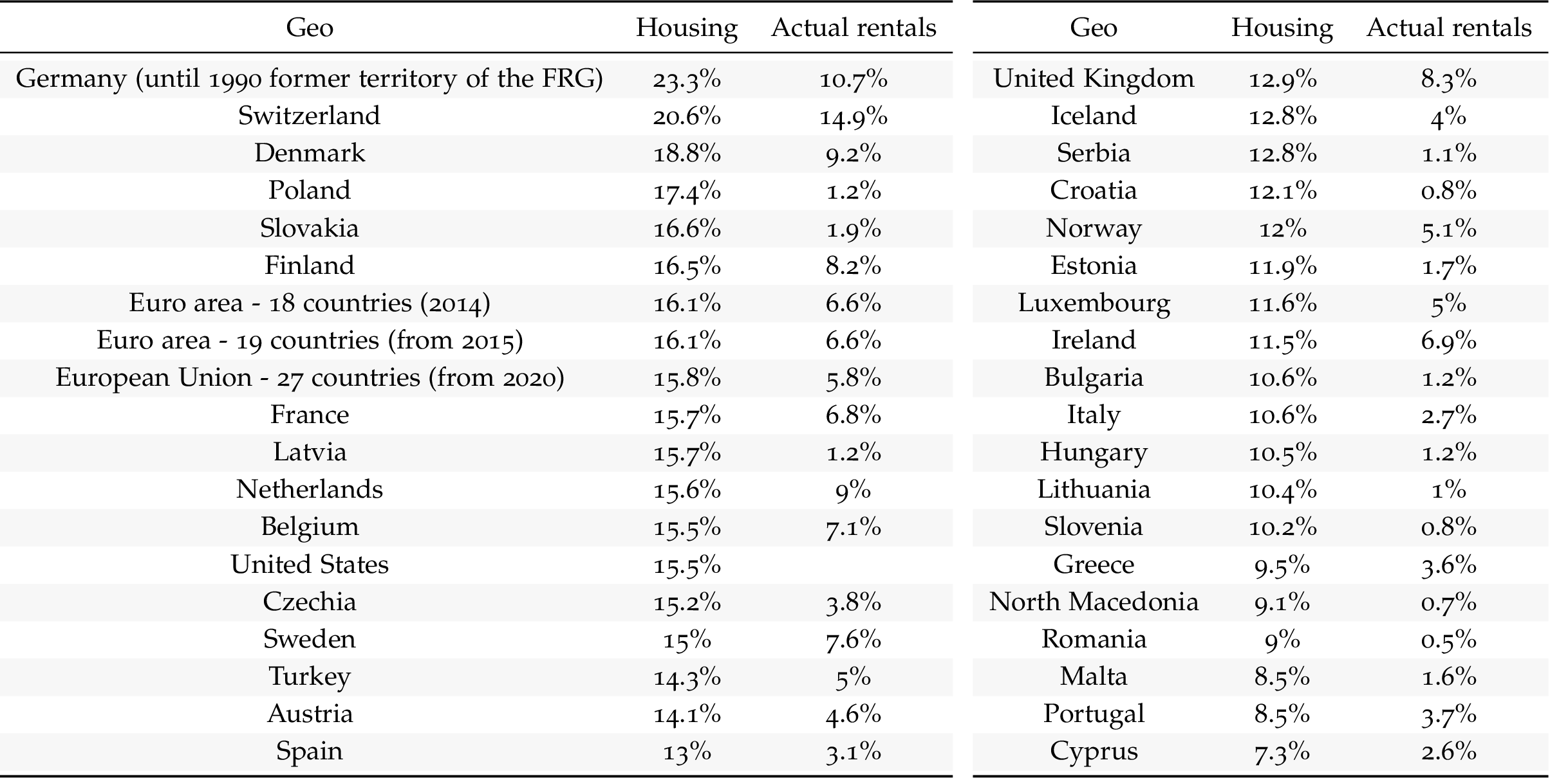
i_g("data/eurostat/ilc_lvho02_files/figure-html/rent-share-CP041-correlation-1.png")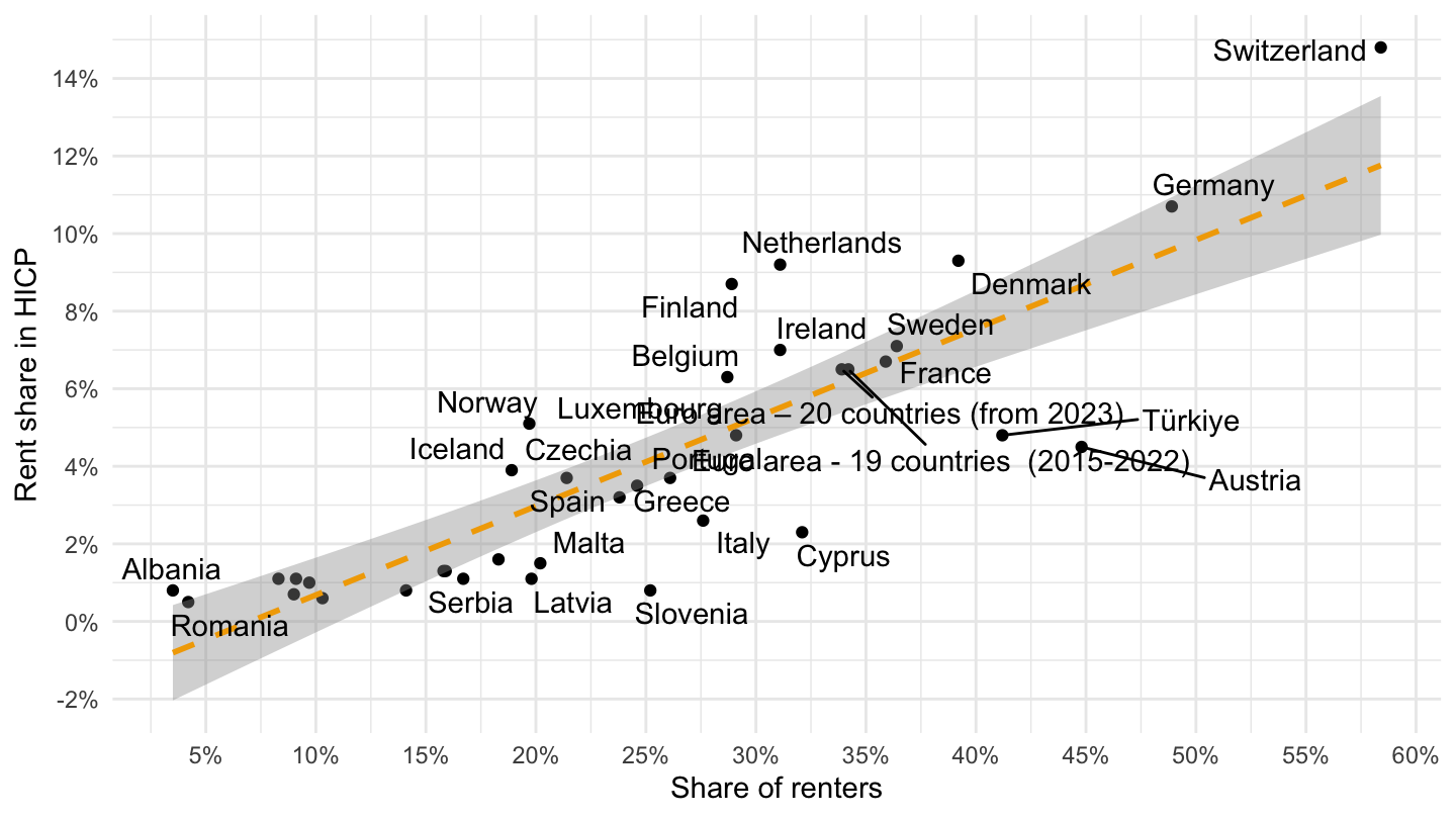
prc_hicp_inw |>
  filter(coicop %in% c("CP04"),
         geo %in% c("FR", "DE", "ES", "IT", "EA19")) |>
  year_to_date() |>

  mutate(values = values/1000) |>
  mutate(Geo = ifelse(geo == "EA19", "Europe", Geo)) |>
  add_flag_color("Geo") |>
  ggplot() + theme_minimal() + ylab("Housing, water, electricity, gas and other fuels ") + xlab("") +
  geom_line(aes(x = date, y = values, color = color)) + add_flags +
  scale_color_identity() +
  scale_x_date(breaks = seq(1920, 2100, 2) |> paste0("-01-01") |> as.Date(),
               labels = date_format("%Y")) +
  scale_y_continuous(breaks = seq(0, 1, 0.01),
               labels = percent_format(a = 1))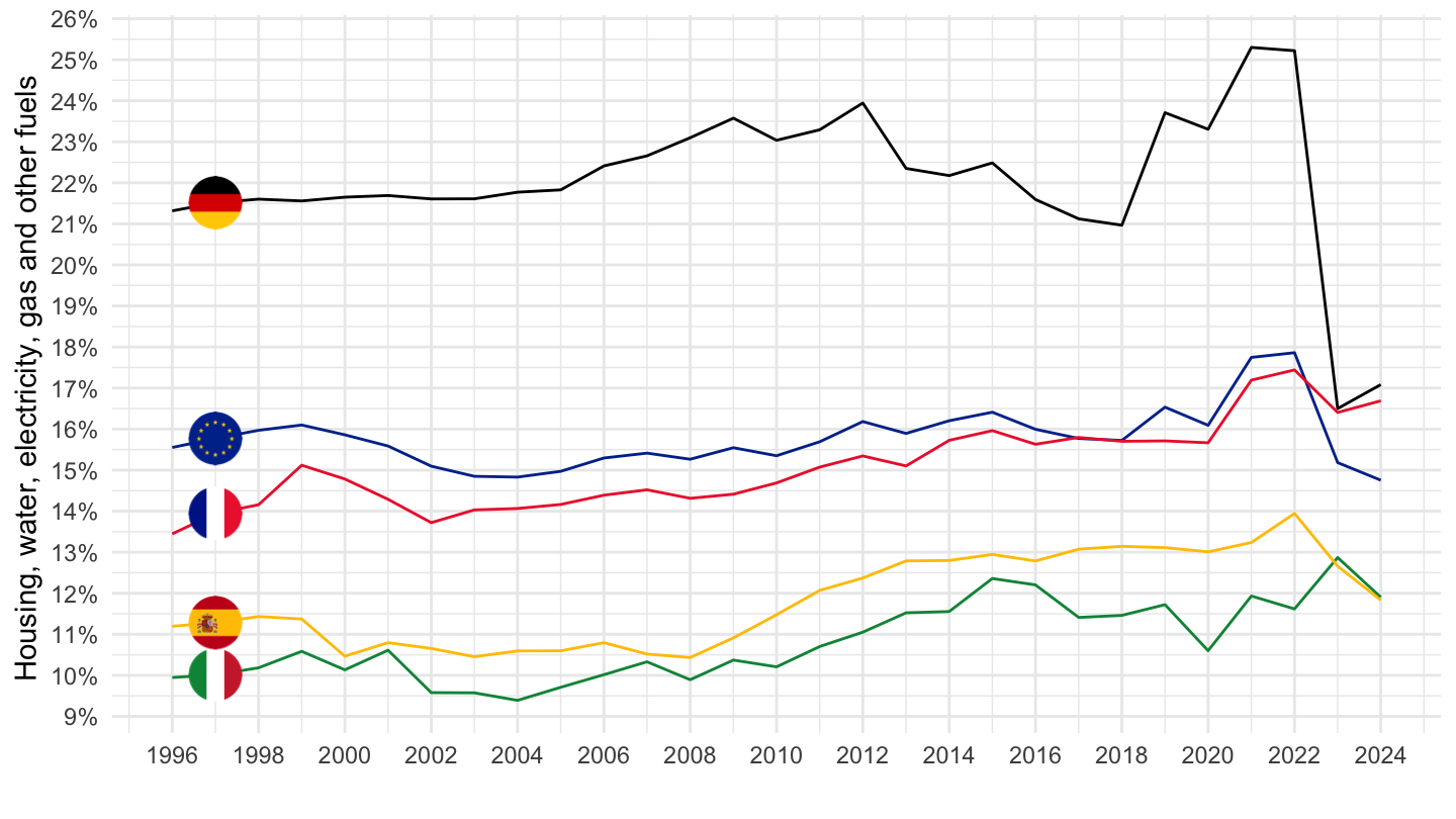
prc_hicp_inw |>
  filter(coicop %in% c("CP041"),
         geo %in% c("FR", "DE", "ES", "IT", "EA19")) |>
  year_to_date() |>

  mutate(values = values/1000) |>
  mutate(Geo = ifelse(geo == "EA19", "Europe", Geo)) |>
  add_flag_color("Geo") |>
  ggplot() + theme_minimal() + ylab("Actual rentals for housing") + xlab("") +
  geom_line(aes(x = date, y = values, color = color)) + add_flags +
  scale_color_identity() +
  scale_x_date(breaks = seq(1920, 2100, 2) |> paste0("-01-01") |> as.Date(),
               labels = date_format("%Y")) +
  theme(legend.position = c(0.45, 0.7),
        legend.title = element_blank()) +
  scale_y_continuous(breaks = seq(0, 1, 0.01),
               labels = percent_format(a = 1))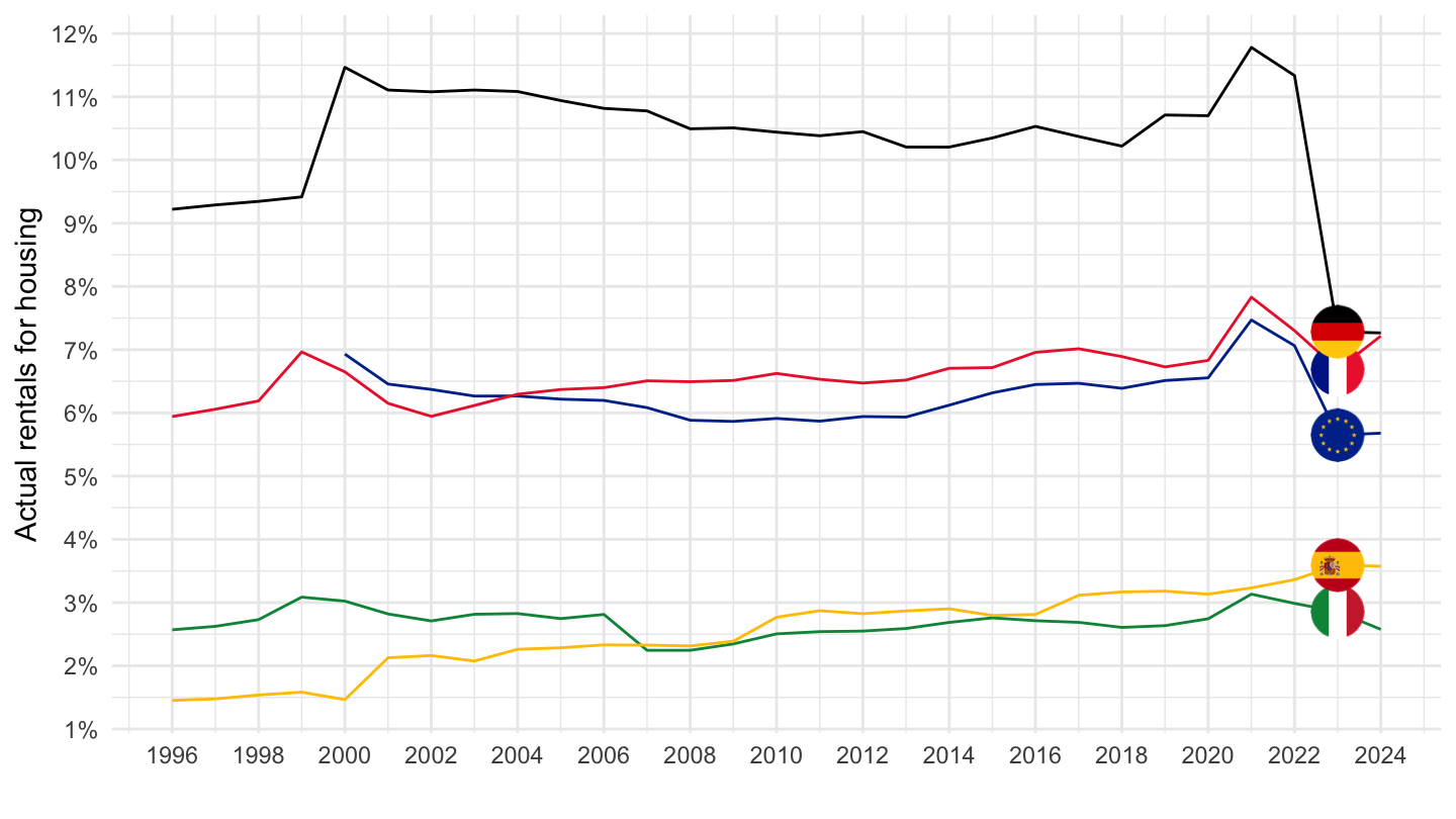
prc_hicp_inw |>
  filter(coicop %in% c("CP10"),
         geo %in% c("FR", "DE", "ES", "IT", "EA19")) |>
  year_to_date() |>

  mutate(values = values/1000) |>
  mutate(Geo = ifelse(geo == "EA19", "Europe", Geo)) |>
  add_flag_color("Geo") |>
  ggplot() + theme_minimal() + ylab("CP10 - Education") + xlab("") +
  geom_line(aes(x = date, y = values, color = color)) + add_flags +
  scale_color_identity() +
  scale_x_date(breaks = seq(1920, 2100, 2) |> paste0("-01-01") |> as.Date(),
               labels = date_format("%Y")) +
  theme(legend.position = c(0.45, 0.7),
        legend.title = element_blank()) +
  scale_y_continuous(breaks = 0.01*seq(0, 10, 0.1),
               labels = percent_format(a = .1))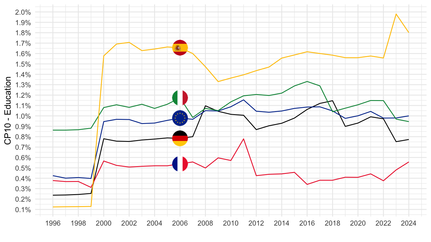
prc_hicp_inw |>
  filter(coicop %in% c("CP071"),
         geo %in% c("FR", "DE", "IT")) |>
  year_to_date() |>

  mutate(values = values/1000) |>
  add_flag_color("Geo") |>
  ggplot() + theme_minimal() + ylab("CP071") + xlab("") +
  geom_line(aes(x = date, y = values, color = color)) + add_flags +
  scale_color_identity() +
  scale_x_date(breaks = seq(1920, 2100, 2) |> paste0("-01-01") |> as.Date(),
               labels = date_format("%Y")) +
  theme(legend.position = c(0.45, 0.7),
        legend.title = element_blank()) +
  scale_y_continuous(breaks = 0.01*seq(0, 10, 0.1),
               labels = percent_format(a = .1))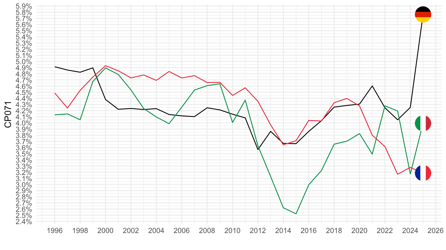
prc_hicp_inw |>
  filter(coicop %in% c("CP0711"),
         geo %in% c("FR", "DE", "IT")) |>
  year_to_date() |>

  mutate(values = values/1000) |>
  add_flag_color("Geo") |>
  ggplot() + theme_minimal() + ylab("CP0711") + xlab("") +
  geom_line(aes(x = date, y = values, color = color)) + add_flags +
  scale_color_identity() +
  scale_x_date(breaks = seq(1920, 2100, 2) |> paste0("-01-01") |> as.Date(),
               labels = date_format("%Y")) +
  theme(legend.position = c(0.45, 0.7),
        legend.title = element_blank()) +
  scale_y_continuous(breaks = 0.01*seq(0, 10, 0.1),
               labels = percent_format(a = .1))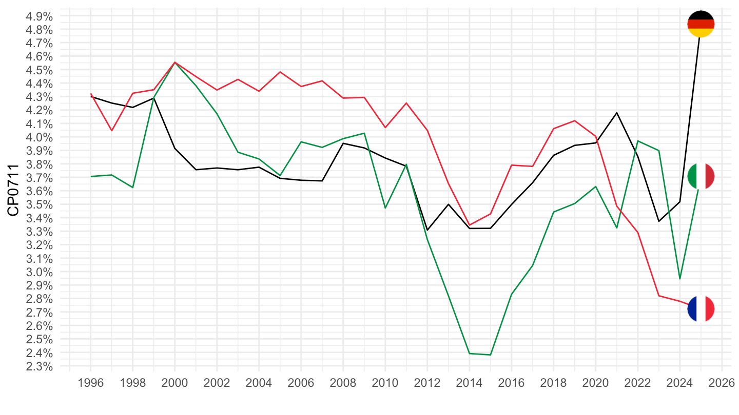
prc_hicp_inw |>
  filter(coicop %in% c("CP0712"),
         geo %in% c("FR", "DE", "IT")) |>
  year_to_date() |>

  mutate(values = values/1000) |>
  add_flag_color("Geo") |>
  ggplot() + theme_minimal() + ylab("CP0712") + xlab("") +
  geom_line(aes(x = date, y = values, color = color)) + add_flags +
  scale_color_identity() +
  scale_x_date(breaks = seq(1920, 2100, 2) |> paste0("-01-01") |> as.Date(),
               labels = date_format("%Y")) +
  theme(legend.position = c(0.45, 0.7),
        legend.title = element_blank()) +
  scale_y_continuous(breaks = 0.01*seq(0, 10, 0.1),
               labels = percent_format(a = .1))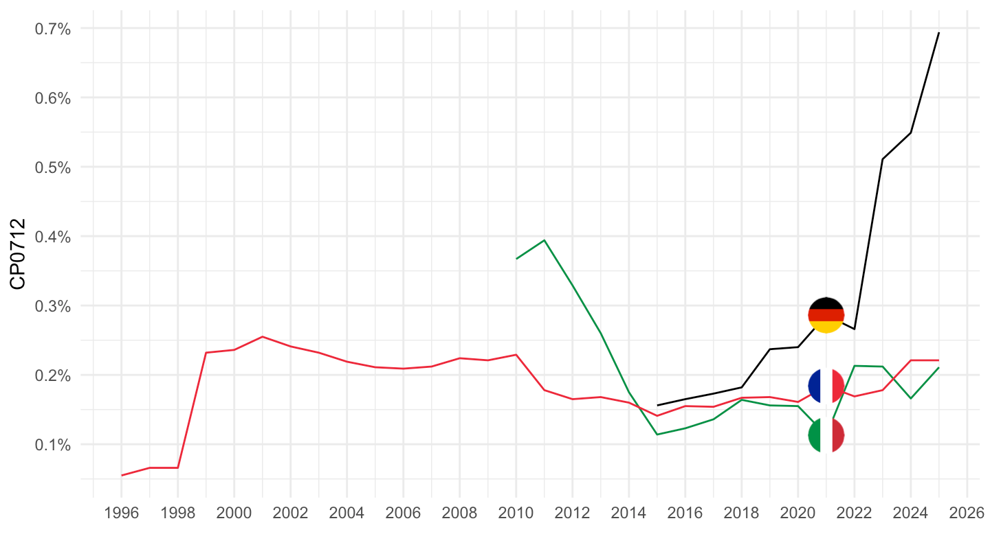
prc_hicp_inw |>
  filter(coicop %in% c("CP07111", "CP07112"),
         geo %in% c("FR", "DE", "IT", "EA20")) |>
  year_to_date() |>


  mutate(values = values/1000) |>
  add_flag_color("Geo") |>
  ggplot() + theme_minimal() + ylab("") + xlab("") +
  geom_line(aes(x = date, y = values, color = color, linetype = paste0(coicop , " - ", Coicop))) + add_flags +
  scale_color_identity() +
  scale_x_date(breaks = seq(1920, 2100, 2) |> paste0("-01-01") |> as.Date(),
               labels = date_format("%Y")) +
  theme(legend.position = c(0.45, 0.7),
        legend.title = element_blank()) +
  scale_y_continuous(breaks = 0.01*seq(0, 10, 0.2),
               labels = percent_format(a = .1))
prc_hicp_inw |>
  filter(coicop %in% c("CP0712", "CP0711"),
         geo %in% c("FR", "DE", "IT")) |>
  year_to_date() |>


  mutate(values = values/1000) |>
  add_flag_color("Geo") |>
  ggplot() + theme_minimal() + ylab("CP0712") + xlab("") +
  geom_line(aes(x = date, y = values, color = color, linetype = Coicop)) + add_flags +
  scale_color_identity() +
  scale_x_date(breaks = seq(1920, 2100, 2) |> paste0("-01-01") |> as.Date(),
               labels = date_format("%Y")) +
  theme(legend.position = c(0.45, 0.7),
        legend.title = element_blank()) +
  scale_y_continuous(breaks = 0.01*seq(0, 10, 0.1),
               labels = percent_format(a = .1))
prc_hicp_inw |>
  filter(coicop %in% c("CP0820"),
         geo %in% c("FR", "DE", "IT")) |>
  year_to_date() |>

  mutate(values = values/1000) |>
  add_flag_color("Geo") |>
  ggplot() + theme_minimal() + ylab("CP0820") + xlab("") +
  geom_line(aes(x = date, y = values, color = color)) + add_flags +
  scale_color_identity() +
  scale_x_date(breaks = seq(1920, 2100, 2) |> paste0("-01-01") |> as.Date(),
               labels = date_format("%Y")) +
  theme(legend.position = c(0.45, 0.7),
        legend.title = element_blank()) +
  scale_y_continuous(breaks = 0.01*seq(0, 10, 0.1),
               labels = percent_format(a = .1))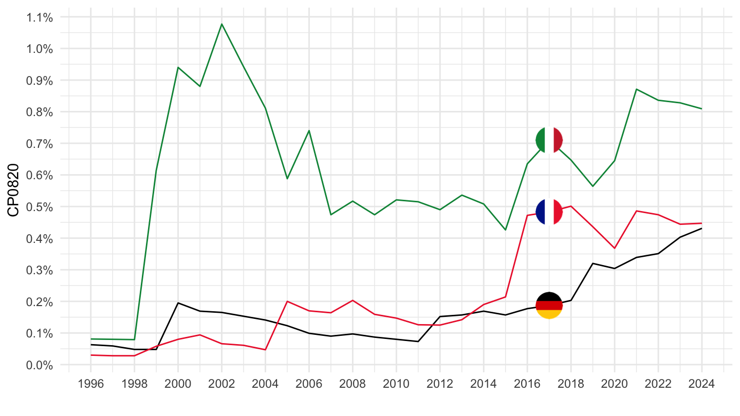
prc_hicp_inw |>
  filter(coicop %in% c("CP091"),
         geo %in% c("FR", "DE", "IT")) |>
  year_to_date() |>

  mutate(values = values/1000) |>
  add_flag_color("Geo") |>
  ggplot() + theme_minimal() + ylab("CP091") + xlab("") +
  geom_line(aes(x = date, y = values, color = color)) + add_flags +
  scale_color_identity() +
  scale_x_date(breaks = seq(1920, 2100, 2) |> paste0("-01-01") |> as.Date(),
               labels = date_format("%Y")) +
  theme(legend.position = c(0.45, 0.7),
        legend.title = element_blank()) +
  scale_y_continuous(breaks = 0.01*seq(0, 10, 0.1),
               labels = percent_format(a = .1))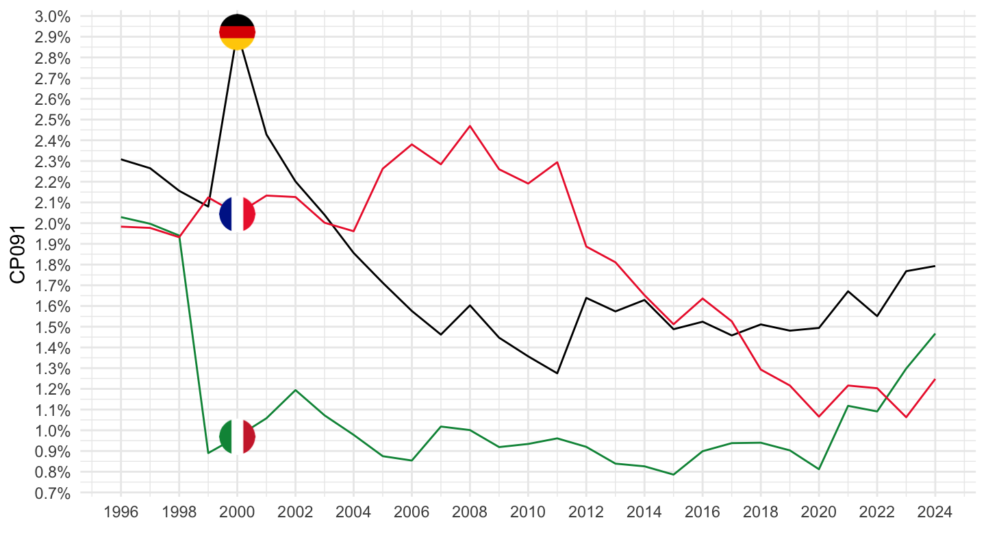
prc_hicp_inw |>
  filter(coicop %in% c("CP092"),
         geo %in% c("FR", "DE", "IT")) |>
  year_to_date() |>

  mutate(values = values/1000) |>
  add_flag_color("Geo") |>
  ggplot() + theme_minimal() + ylab("CP092") + xlab("") +
  geom_line(aes(x = date, y = values, color = color)) + add_flags +
  scale_color_identity() +
  scale_x_date(breaks = seq(1920, 2100, 2) |> paste0("-01-01") |> as.Date(),
               labels = date_format("%Y")) +
  theme(legend.position = c(0.45, 0.7),
        legend.title = element_blank()) +
  scale_y_continuous(breaks = 0.01*seq(0, 10, 0.1),
               labels = percent_format(a = .1))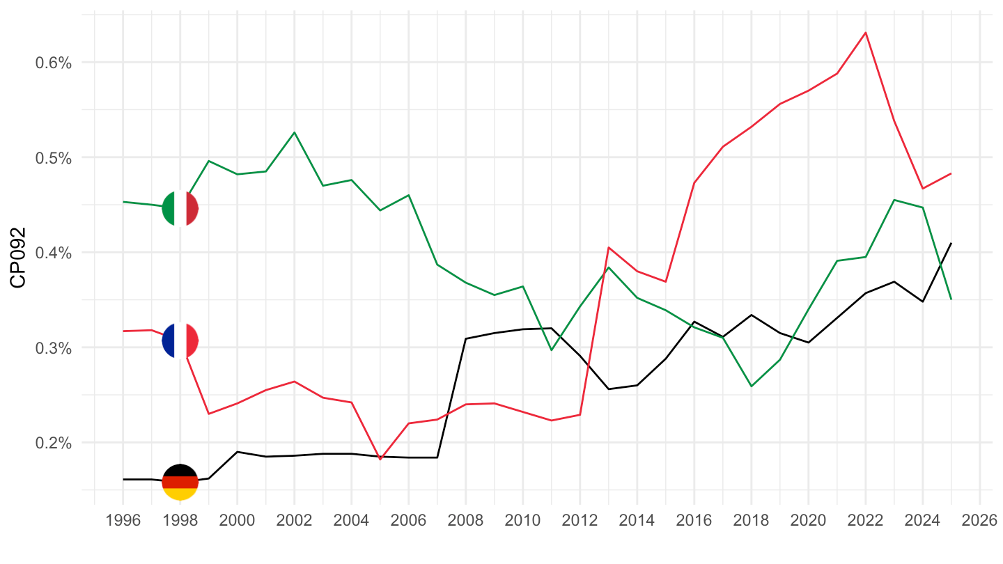
prc_hicp_inw |>
  filter(coicop %in% c("CP09211"),
         geo %in% c("FR", "DE", "IT")) |>
  year_to_date() |>

  mutate(values = values/1000) |>
  add_flag_color("Geo") |>
  ggplot() + theme_minimal() + ylab("CP09211") + xlab("") +
  geom_line(aes(x = date, y = values, color = color)) + add_flags +
  scale_color_identity() +
  scale_x_date(breaks = seq(1920, 2100, 2) |> paste0("-01-01") |> as.Date(),
               labels = date_format("%Y")) +
  theme(legend.position = c(0.45, 0.7),
        legend.title = element_blank()) +
  scale_y_continuous(breaks = 0.01*seq(0, 10, 0.1),
               labels = percent_format(a = .1))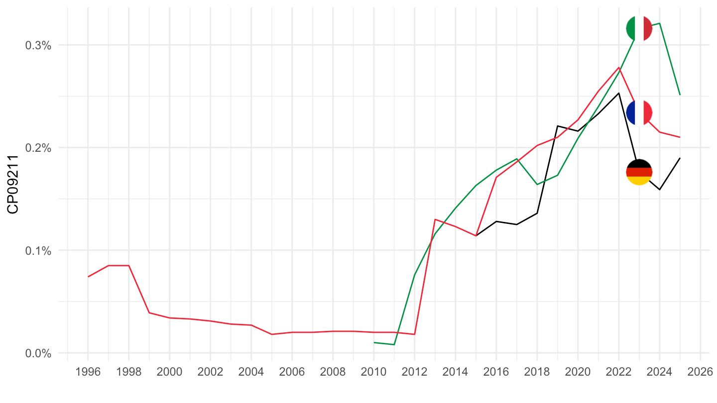
prc_hicp_inw |>
  filter(coicop %in% c("CP0921"),
         geo %in% c("FR", "DE", "IT")) |>
  year_to_date() |>

  mutate(values = values/1000) |>
  add_flag_color("Geo") |>
  ggplot() + theme_minimal() + ylab("CP0921") + xlab("") +
  geom_line(aes(x = date, y = values, color = color)) + add_flags +
  scale_color_identity() +
  scale_x_date(breaks = seq(1920, 2100, 2) |> paste0("-01-01") |> as.Date(),
               labels = date_format("%Y")) +
  theme(legend.position = c(0.45, 0.7),
        legend.title = element_blank()) +
  scale_y_continuous(breaks = 0.01*seq(0, 10, 0.1),
               labels = percent_format(a = .1))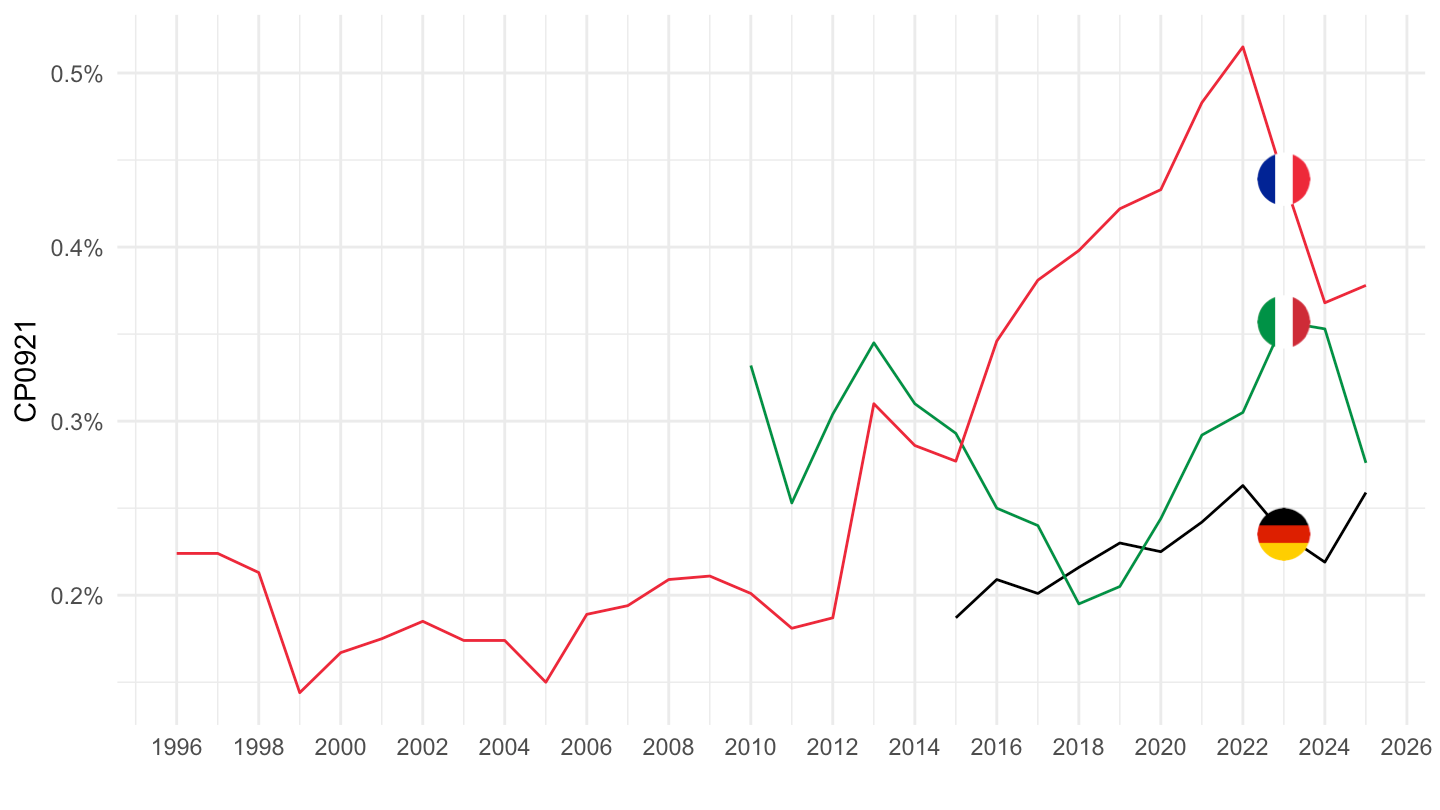
prc_hicp_inw |>
  filter(coicop %in% c("CP0921", "CP0922", "CP0923"),
         geo %in% c("FR")) |>
  year_to_date() |>

  mutate(values = values/1000) |>
  ggplot() + theme_minimal() + ylab("CP092") + xlab("") +
  geom_line(aes(x = date, y = values, color = Coicop)) +
  scale_x_date(breaks = seq(1920, 2100, 2) |> paste0("-01-01") |> as.Date(),
               labels = date_format("%Y")) +
  theme(legend.position = c(0.45, 0.7),
        legend.title = element_blank()) +
  scale_y_continuous(breaks = 0.01*seq(0, 10, 0.1),
               labels = percent_format(a = .1))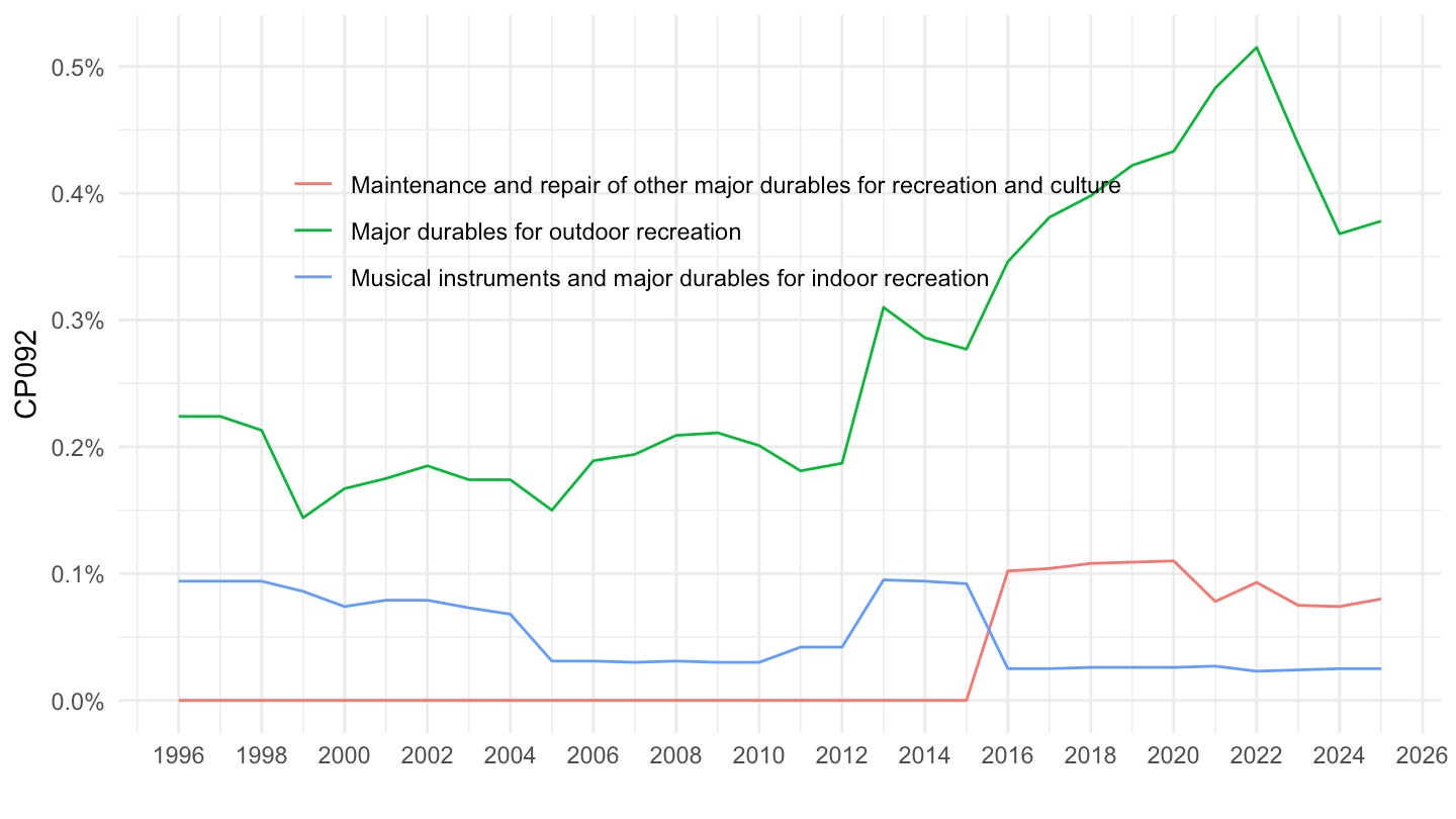
prc_hicp_inw |>
  filter(coicop %in% c("CP10"),
         geo %in% c("FR", "DE", "IT")) |>
  year_to_date() |>

  mutate(values = values/1000) |>
  add_flag_color("Geo") |>
  ggplot() + theme_minimal() + ylab("CP10 - Education") + xlab("") +
  geom_line(aes(x = date, y = values, color = color)) + add_flags +
  scale_color_identity() +
  scale_x_date(breaks = seq(1920, 2100, 2) |> paste0("-01-01") |> as.Date(),
               labels = date_format("%Y")) +
  theme(legend.position = c(0.45, 0.7),
        legend.title = element_blank()) +
  scale_y_continuous(breaks = 0.01*seq(0, 10, 0.1),
               labels = percent_format(a = .1))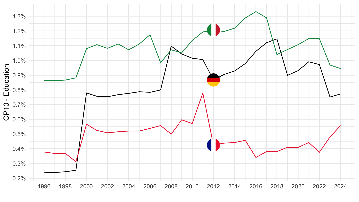
prc_hicp_inw |>
  filter(coicop %in% c("CP06"),
         geo %in% c("FR", "DE", "IT")) |>
  year_to_date() |>

  mutate(values = values/1000) |>
  add_flag_color("Geo") |>
  ggplot() + theme_minimal() + ylab("Health ") + xlab("") +
  geom_line(aes(x = date, y = values, color = color)) + add_flags +
  scale_color_identity() +
  scale_x_date(breaks = seq(1920, 2100, 2) |> paste0("-01-01") |> as.Date(),
               labels = date_format("%Y")) +
  theme(legend.position = c(0.45, 0.7),
        legend.title = element_blank()) +
  scale_y_continuous(breaks = seq(0, 1, 0.01),
               labels = percent_format(a = 1))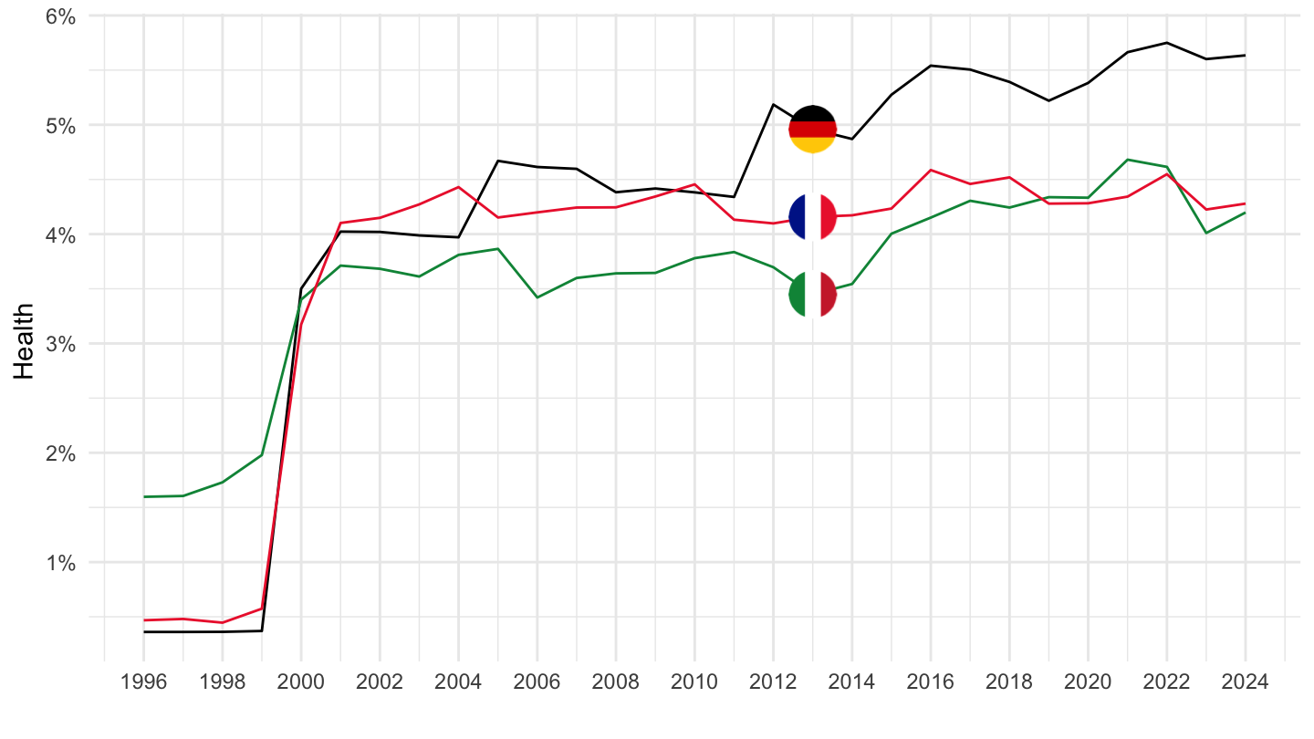
prc_hicp_inw |>
  filter(coicop %in% c("CP061"),
         geo %in% c("FR", "DE", "IT")) |>
  year_to_date() |>

  mutate(values = values/1000) |>
  add_flag_color("Geo") |>
  ggplot() + theme_minimal() + ylab("Health ") + xlab("") +
  geom_line(aes(x = date, y = values, color = color)) + add_flags +
  scale_color_identity() +
  scale_x_date(breaks = seq(1920, 2100, 2) |> paste0("-01-01") |> as.Date(),
               labels = date_format("%Y")) +
  theme(legend.position = c(0.45, 0.7),
        legend.title = element_blank()) +
  scale_y_continuous(breaks = seq(0, 1, 0.01),
               labels = percent_format(a = 1))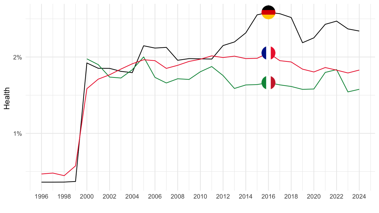
prc_hicp_inw |>
  filter(coicop %in% c("CP062"),
         geo %in% c("FR", "DE", "IT")) |>
  year_to_date() |>

  mutate(values = values/1000) |>
  add_flag_color("Geo") |>
  ggplot() + theme_minimal() + ylab("Health ") + xlab("") +
  geom_line(aes(x = date, y = values, color = color)) + add_flags +
  scale_color_identity() +
  scale_x_date(breaks = seq(1920, 2100, 2) |> paste0("-01-01") |> as.Date(),
               labels = date_format("%Y")) +
  theme(legend.position = c(0.45, 0.7),
        legend.title = element_blank()) +
  scale_y_continuous(breaks = seq(0, 1, 0.01),
               labels = percent_format(a = 1))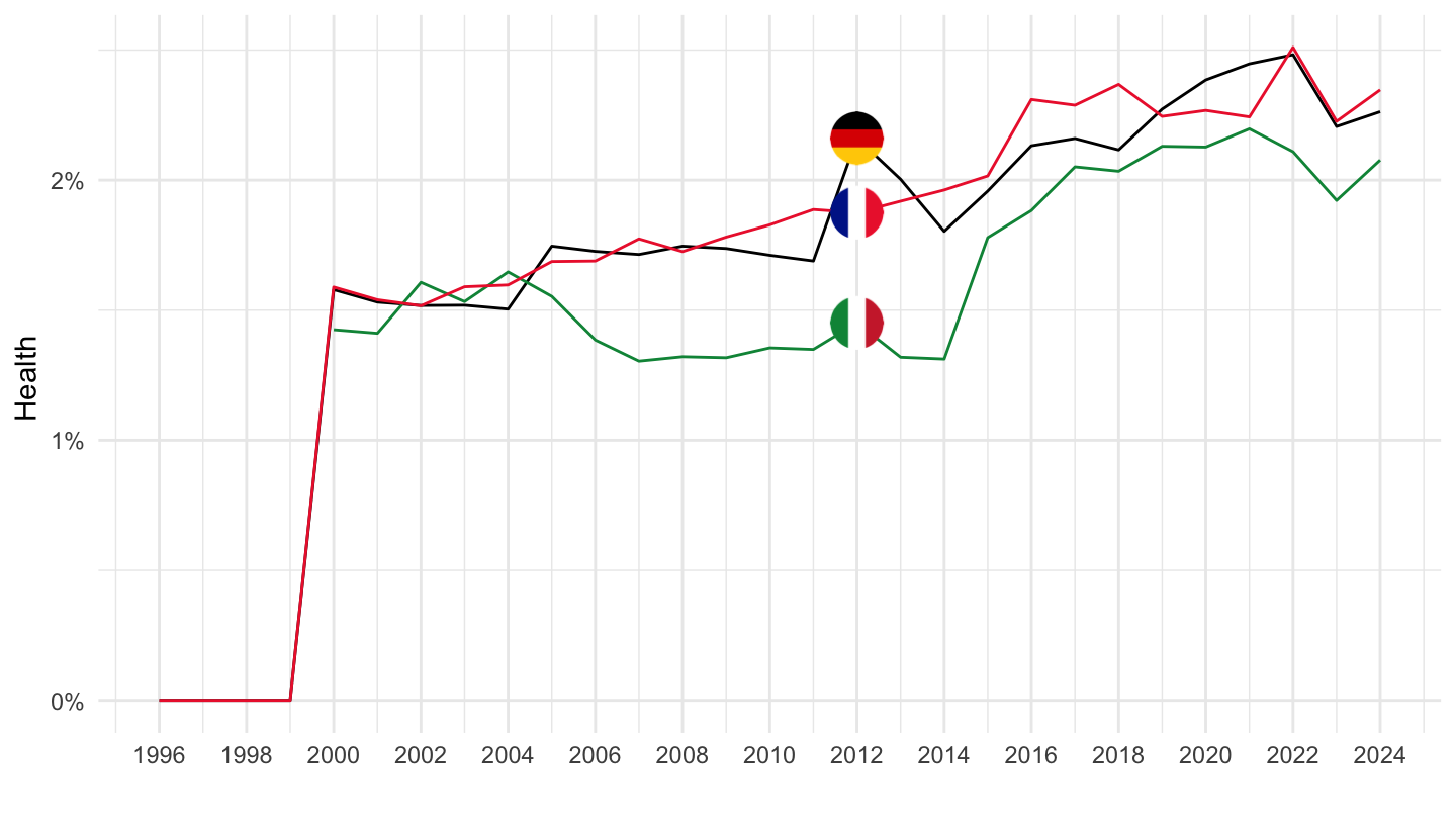
prc_hicp_inw |>
  filter(coicop %in% c("CP063"),
         geo %in% c("FR", "DE", "IT")) |>
  year_to_date() |>

  mutate(values = values/1000) |>
  add_flag_color("Geo") |>
  ggplot() + theme_minimal() + ylab("Health ") + xlab("") +
  geom_line(aes(x = date, y = values, color = color)) + add_flags +
  scale_color_identity() +
  scale_x_date(breaks = seq(1920, 2100, 2) |> paste0("-01-01") |> as.Date(),
               labels = date_format("%Y")) +
  theme(legend.position = c(0.45, 0.7),
        legend.title = element_blank()) +
  scale_y_continuous(breaks = seq(0, 1, 0.001),
               labels = percent_format(a = .1))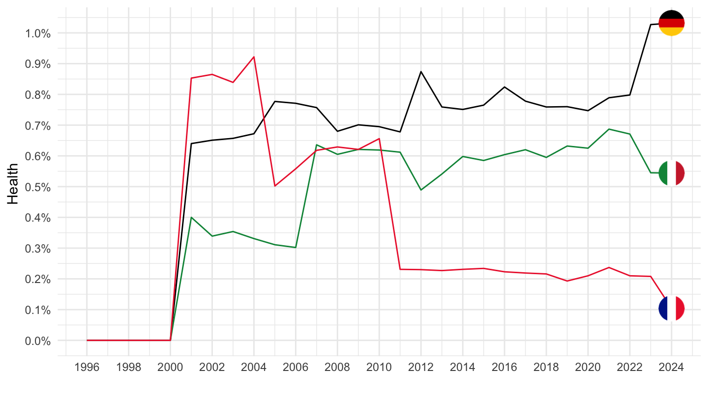
| source | dataset | Title | Updated |
|---|---|---|---|

