| source | dataset | Title | .html | .rData |
|---|---|---|---|---|
| bis | SELECTED_PP | Property prices, selected series | 2026-07-24 | 2026-07-24 |
Property prices, selected series
Data - BIS
Info
Data on housing
| source | dataset | Title | .html | .rData |
|---|---|---|---|---|
| bis | SELECTED_PP | Property prices, selected series | 2026-07-24 | 2026-07-24 |
| bdf | RPP | Prix de l'immobilier | 2026-07-24 | 2026-07-24 |
| bis | LONG_PP | Residential property prices - detailed series | 2026-07-24 | 2024-05-10 |
| ecb | RPP | Residential Property Price Index Statistics | 2026-07-24 | 2026-07-24 |
| eurostat | ei_hppi_q | House price index (2015 = 100) - quarterly data | 2026-07-23 | 2026-07-23 |
| eurostat | hbs_str_t223 | Mean consumption expenditure by income quintile | 2025-10-11 | 2026-07-23 |
| eurostat | prc_hicp_midx | HICP (2015 = 100) - monthly data (index) | 2026-07-24 | 2026-07-23 |
| eurostat | prc_hpi_q | House price index (2015 = 100) - quarterly data | 2026-07-24 | 2026-07-23 |
| fred | housing | House Prices | 2026-07-24 | 2026-07-24 |
| insee | IPLA-IPLNA-2015 | Indices des prix des logements neufs et Indices Notaires-Insee des prix des logements anciens | 2026-07-24 | 2026-07-23 |
| oecd | SNA_TABLE5 | Final consumption expenditure of households | 2026-07-24 | 2023-10-19 |
| oecd | housing | NA | NA | NA |
LAST_COMPILE
| LAST_COMPILE |
|---|
| 2026-07-25 |
Last
Code
SELECTED_PP %>%
  group_by(date) %>%
  summarise(Nobs = n()) %>%
  arrange(desc(date)) %>%
  head(1) %>%
print_table_conditional()| date | Nobs |
|---|---|
| 2023-09-30 | 248 |
Nobs
Code
SELECTED_PP %>%
  arrange(iso3c, FREQ, date) %>%
  group_by(iso3c, FREQ, VALUE, `Reference area`) %>%
  summarise(Nobs = n(),
            start = first(date),
            end = last(date)) %>%
  arrange(-Nobs) %>%
  mutate(Flag = gsub(" ", "-", str_to_lower(`Reference area`)),
         Flag = paste0('<img src="../../icon/flag/vsmall/', Flag, '.png" alt="Flag">')) %>%
  select(Flag, everything()) %>%
  {if (is_html_output()) datatable(., filter = 'top', rownames = F, escape = F) else .}
iso3c, Reference area
Code
SELECTED_PP %>%
  arrange(iso3c, date) %>%
  group_by(iso3c, `Reference area`) %>%
  summarise(Nobs = n(),
            start = first(date),
            end = last(date)) %>%
  arrange(-Nobs) %>%
  mutate(Flag = gsub(" ", "-", str_to_lower(`Reference area`)),
         Flag = paste0('<img src="../../icon/flag/vsmall/', Flag, '.png" alt="Flag">')) %>%
  select(Flag, everything()) %>%
  {if (is_html_output()) datatable(., filter = 'top', rownames = F, escape = F) else .}
VALUE, Value
Code
SELECTED_PP %>%
  group_by(VALUE, Value) %>%
  summarise(Nobs = n()) %>%
  arrange(-Nobs) %>%
print_table_conditional()| VALUE | Value | Nobs |
|---|---|---|
| N | Nominal | 47988 |
| R | Real | 47988 |
UNIT_MEASURE, Unit of measure
Code
SELECTED_PP %>%
  group_by(UNIT_MEASURE, `Unit of measure`) %>%
  summarise(Nobs = n()) %>%
  arrange(-Nobs) %>%
print_table_conditional()| UNIT_MEASURE | Unit of measure | Nobs |
|---|---|---|
| 628 | Index, 2010 = 100 | 47988 |
| 771 | Year-on-year changes, in per cent | 47988 |
FREQ, Frequency
Code
SELECTED_PP %>%
  group_by(FREQ, Frequency) %>%
  summarise(Nobs = n()) %>%
  arrange(-Nobs) %>%
print_table_conditional()| FREQ | Frequency | Nobs |
|---|---|---|
| Q | Quarterly | 95976 |
date
Code
SELECTED_PP %>%
  group_by(date) %>%
  summarise(Nobs = n()) %>%
  arrange(desc(date)) %>%
  print_table_conditional()
Real House Prices
Thailand, South Korea, Japan
All
Code
SELECTED_PP %>%
  filter(iso3c %in% c("JPN", "KOR", "THA"),
         FREQ == "Q",
         VALUE == "R",
         UNIT_MEASURE == 628) %>%
  left_join(colors, by = c("Reference area" = "country")) %>%
  ggplot(.) + theme_minimal() + xlab("") + ylab("Real House Prices (Index, 2010 = 100)") +
  geom_line(aes(x = date, y = value, color = color)) +
  scale_color_identity() + add_flags +
  scale_x_date(breaks = seq(1900, 2100, 5) %>% paste0("-01-01") %>% as.Date,
               labels = date_format("%Y")) +
  scale_y_log10(breaks = seq(0, 600, 10),
                     labels = dollar_format(a = 1, prefix = "")) +
  theme(legend.position = c(0.8, 0.2),
        legend.title = element_blank())
1975
Code
SELECTED_PP %>%
  filter(iso3c %in% c("JPN", "KOR", "THA"),
         FREQ == "Q",
         date >= as.Date("1980-01-01"),
         VALUE == "R",
         UNIT_MEASURE == 628) %>%
  left_join(colors, by = c("Reference area" = "country")) %>%
  ggplot(.) + theme_minimal() + xlab("") + ylab("Real House Prices (Index, 2010 = 100)") +
  geom_line(aes(x = date, y = value, color = color)) +
  scale_color_identity() + add_flags +
  scale_x_date(breaks = seq(1900, 2100, 5) %>% paste0("-01-01") %>% as.Date,
               labels = date_format("%Y")) +
  scale_y_log10(breaks = seq(0, 600, 10),
                     labels = dollar_format(a = 1, prefix = "")) +
  theme(legend.position = c(0.8, 0.2),
        legend.title = element_blank())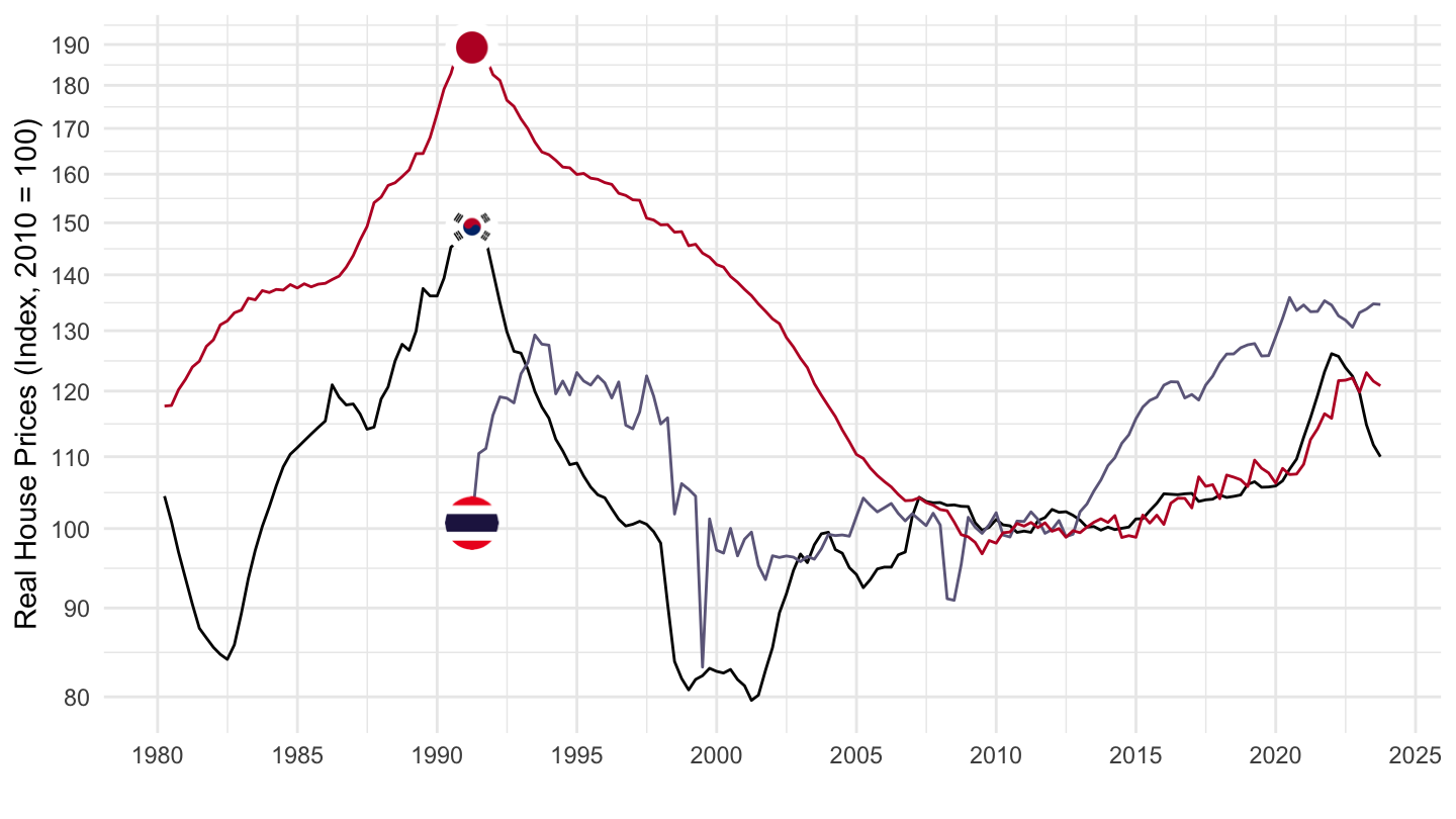
1990-
Code
SELECTED_PP %>%
  filter(iso3c %in% c("JPN", "KOR", "THA"),
         FREQ == "Q",
         date >= as.Date("1990-01-01") - days(1),
         VALUE == "R",
         UNIT_MEASURE == 628) %>%
  left_join(colors, by = c("Reference area" = "country")) %>%
  ggplot(.) + theme_minimal() + xlab("") + ylab("Real House Prices (Index, 2010 = 100)") +
  geom_line(aes(x = date, y = value, color = color)) +
  scale_color_identity() + add_flags +
  scale_x_date(breaks = seq(1900, 2100, 5) %>% paste0("-01-01") %>% as.Date,
               labels = date_format("%Y")) +
  scale_y_log10(breaks = seq(0, 600, 10),
                     labels = dollar_format(a = 1, prefix = "")) +
  theme(legend.position = c(0.8, 0.2),
        legend.title = element_blank())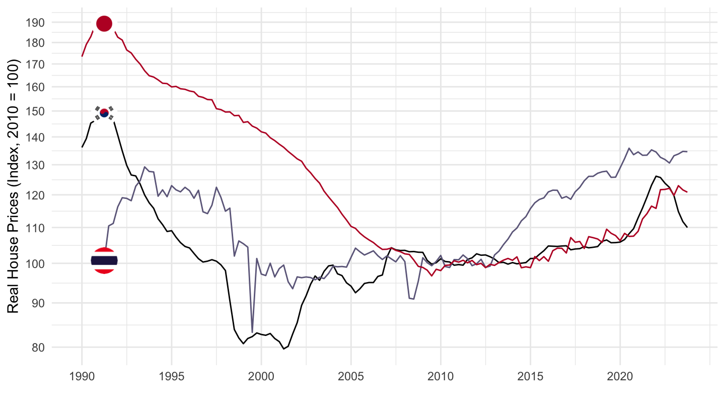
2010-
Code
SELECTED_PP %>%
  filter(iso3c %in% c("JPN", "KOR", "THA"),
         FREQ == "Q",
         date >= as.Date("2009-12-31"),
         VALUE == "R",
         UNIT_MEASURE == 628) %>%
  left_join(colors, by = c("Reference area" = "country")) %>%
  group_by(`Reference area`) %>%
  ggplot(.) + theme_minimal() + xlab("") + ylab("Real House Prices (Index, 2010 = 100)") +
  geom_line(aes(x = date, y = value, color = color)) +
  scale_color_identity() + add_flags +
  scale_x_date(breaks = seq(1900, 2100, 1) %>% paste0("-01-01") %>% as.Date,
               labels = date_format("%Y")) +
  scale_y_log10(breaks = seq(0, 600, 10),
                     labels = dollar_format(a = 1, prefix = "")) +
  theme(legend.position = c(0.8, 0.2),
        legend.title = element_blank())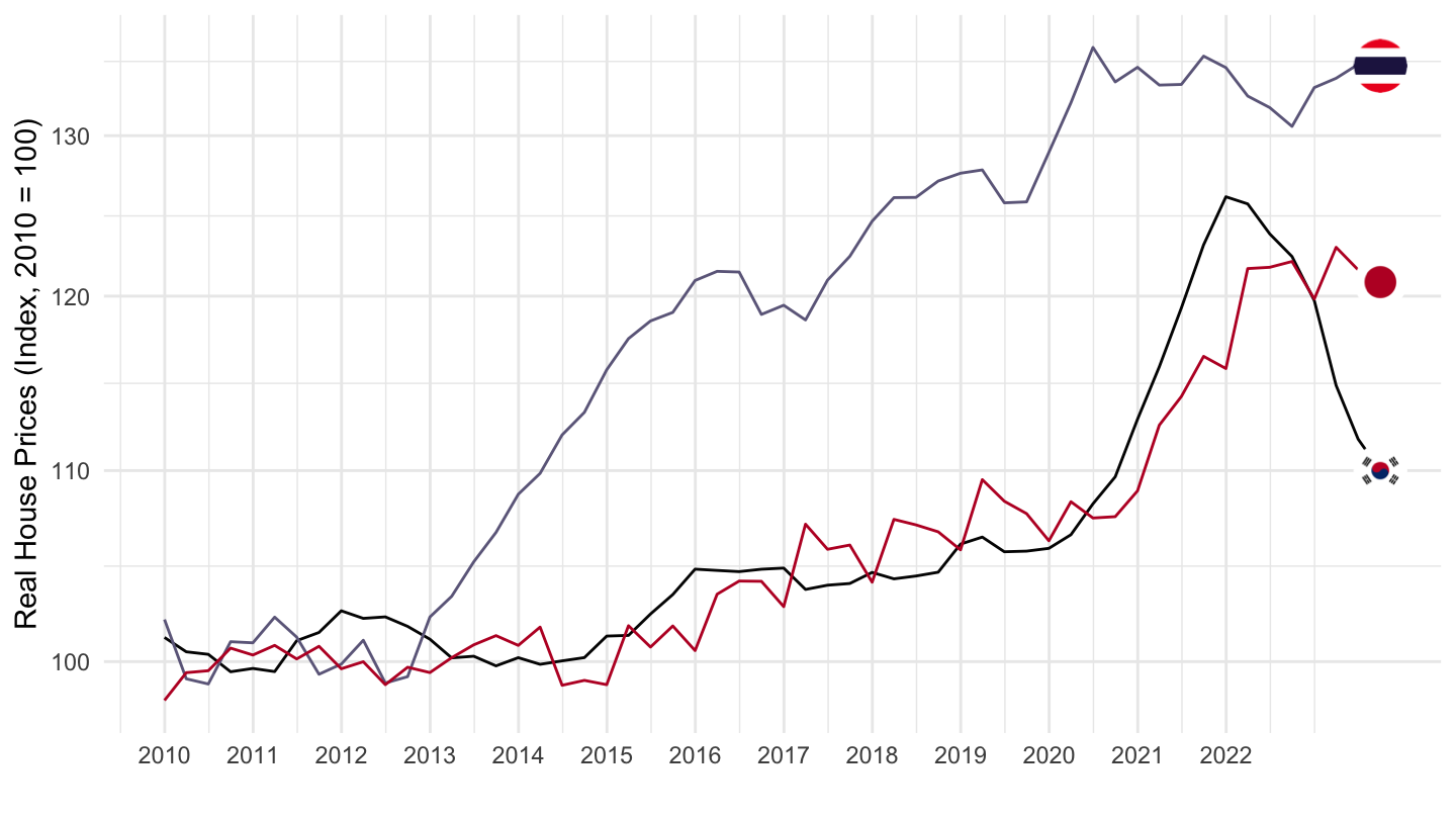
Thailand, Sweden, Japan
All
Code
SELECTED_PP %>%
  filter(iso3c %in% c("JPN", "SWE", "THA"),
         FREQ == "Q",
         date >= as.Date("1970-01-01"),
         VALUE == "R",
         UNIT_MEASURE == 628) %>%
  left_join(colors, by = c("Reference area" = "country")) %>%
  ggplot(.) + theme_minimal() + xlab("") + ylab("Real House Prices (Index, 2010 = 100)") +
  geom_line(aes(x = date, y = value, color = color)) +
  scale_color_identity() + add_flags +
  scale_x_date(breaks = seq(1900, 2100, 5) %>% paste0("-01-01") %>% as.Date,
               labels = date_format("%Y")) +
  scale_y_log10(breaks = seq(0, 600, 10),
                     labels = dollar_format(a = 1, prefix = "")) +
  theme(legend.position = c(0.8, 0.2),
        legend.title = element_blank())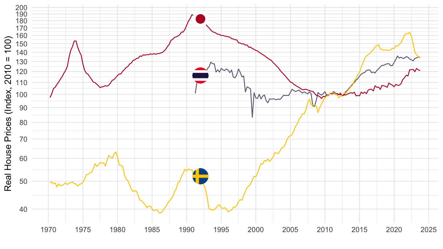
1980-
Code
SELECTED_PP %>%
  filter(iso3c %in% c("JPN", "SWE", "THA"),
         FREQ == "Q",
         date >= as.Date("1980-01-01"),
         VALUE == "R",
         UNIT_MEASURE == 628) %>%
  left_join(colors, by = c("Reference area" = "country")) %>%
  ggplot(.) + theme_minimal() + xlab("") + ylab("Real House Prices (Index, 2010 = 100)") +
  geom_line(aes(x = date, y = value, color = color)) +
  scale_color_identity() + add_flags +
  scale_x_date(breaks = seq(1900, 2100, 5) %>% paste0("-01-01") %>% as.Date,
               labels = date_format("%Y")) +
  scale_y_log10(breaks = seq(0, 600, 10),
                     labels = dollar_format(a = 1, prefix = "")) +
  theme(legend.position = c(0.8, 0.2),
        legend.title = element_blank())
1990-
Code
SELECTED_PP %>%
  filter(iso3c %in% c("JPN", "SWE", "THA"),
         FREQ == "Q",
         date >= as.Date("1990-01-01")-days(1),
         VALUE == "R",
         UNIT_MEASURE == 628) %>%
  left_join(colors, by = c("Reference area" = "country")) %>%
  ggplot(.) + theme_minimal() + xlab("") + ylab("Real House Prices (Index, 2010 = 100)") +
  geom_line(aes(x = date, y = value, color = color)) +
  scale_color_identity() + add_flags +
  scale_x_date(breaks = seq(1900, 2100, 5) %>% paste0("-01-01") %>% as.Date,
               labels = date_format("%Y")) +
  scale_y_log10(breaks = seq(0, 600, 10),
                     labels = dollar_format(a = 1, prefix = "")) +
  theme(legend.position = c(0.8, 0.2),
        legend.title = element_blank())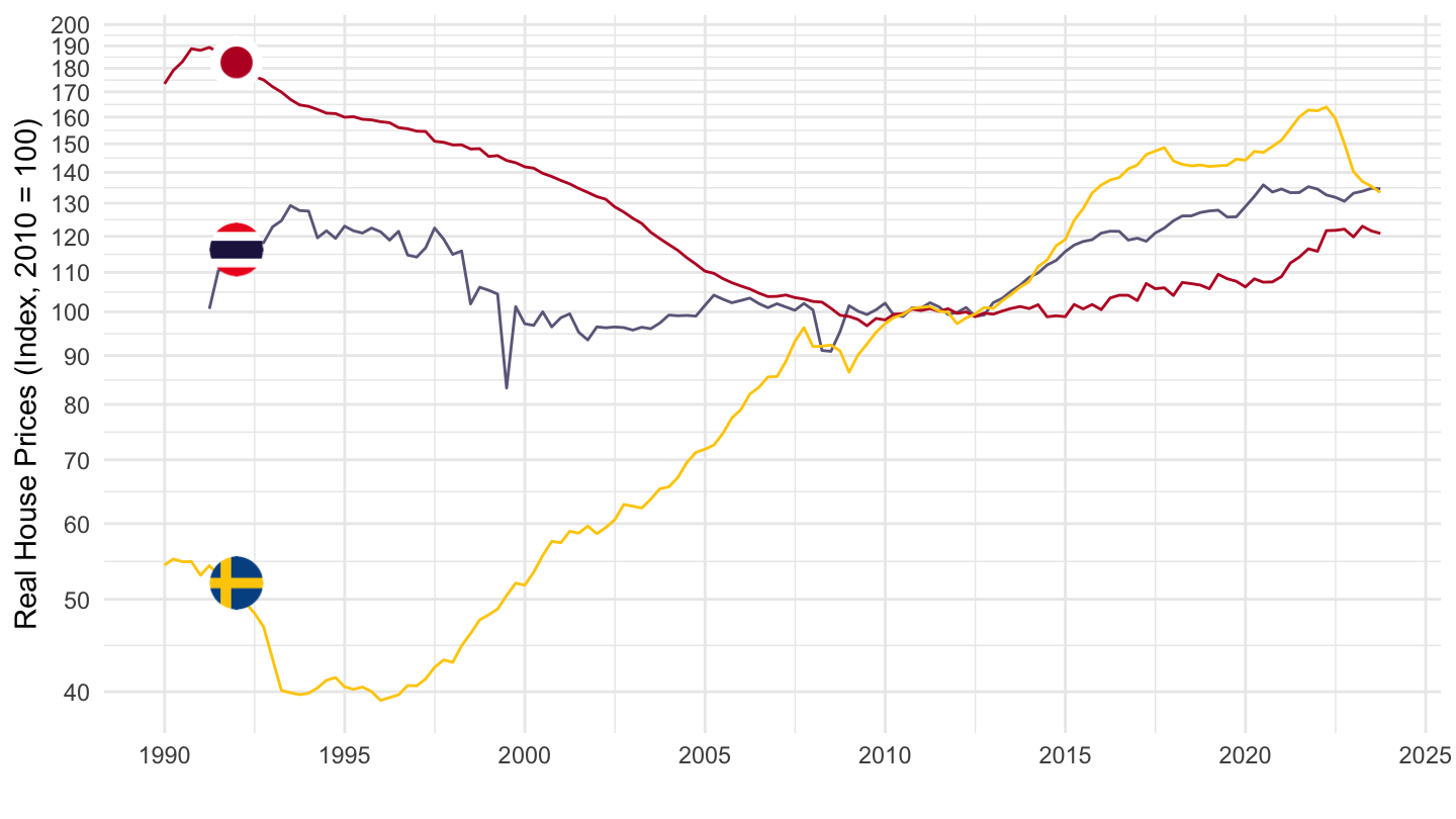
Japan, United States, United Kingdom
Code
SELECTED_PP %>%
  filter(iso3c %in% c("JPN", "GBR", "USA"),
         FREQ == "Q",
         date >= as.Date("1970-01-01"),
         VALUE == "R",
         UNIT_MEASURE == 628) %>%
  left_join(colors, by = c("Reference area" = "country")) %>%
  ggplot(.) + theme_minimal() + xlab("") + ylab("Real House Prices (Index, 2010 = 100)") +
  geom_line(aes(x = date, y = value, color = color)) +
  scale_color_identity() + add_flags +
  scale_x_date(breaks = seq(1900, 2100, 5) %>% paste0("-01-01") %>% as.Date,
               labels = date_format("%Y")) +
  scale_y_log10(breaks = seq(0, 600, 10),
                     labels = dollar_format(a = 1, prefix = "")) +
  theme(legend.position = c(0.8, 0.2),
        legend.title = element_blank())
Germany, France, Italy, Spain, Netherlands
1971-
Code
SELECTED_PP %>%
  filter(iso3c %in% c("DEU", "FRA", "ITA", "ESP", "NLD"),
         FREQ == "Q",
         date >= as.Date("1971-03-31"),
         VALUE == "R",
         UNIT_MEASURE == 628) %>%
  left_join(colors, by = c("Reference area" = "country")) %>%
  mutate(color = ifelse(iso3c == "FRA", color2, color)) %>%
  group_by(iso3c) %>%
  mutate(value = 100*value/value[date == as.Date("1971-03-31")]) %>%
  ggplot(.) + theme_minimal() + xlab("") + ylab("Real House Prices (Index, 1971 = 100)") +
  geom_line(aes(x = date, y = value, color = color)) +
  scale_color_identity() + add_flags +
  scale_x_date(breaks = seq(1900, 2100, 5) %>% paste0("-01-01") %>% as.Date,
               labels = date_format("%Y")) +
  scale_y_log10(breaks = seq(0, 600, 10),
                     labels = dollar_format(a = 1, prefix = "")) +
  theme(legend.position = c(0.8, 0.2),
        legend.title = element_blank())
1990-
Code
SELECTED_PP %>%
  filter(iso3c %in% c("DEU", "FRA", "ITA", "ESP", "NLD"),
         FREQ == "Q",
         date >= as.Date("1989-12-31"),
         VALUE == "R",
         UNIT_MEASURE == 628) %>%
  left_join(colors, by = c("Reference area" = "country")) %>%
  mutate(color = ifelse(iso3c == "FRA", color2, color)) %>%
  group_by(iso3c) %>%
  mutate(value = 100*value/value[date == as.Date("1989-12-31")]) %>%
  ggplot(.) + theme_minimal() + xlab("") + ylab("Real House Prices (Index, 1990 = 100)") +
  geom_line(aes(x = date, y = value, color = color)) +
  scale_color_identity() + add_flags +
  scale_x_date(breaks = seq(1900, 2100, 5) %>% paste0("-01-01") %>% as.Date,
               labels = date_format("%Y")) +
  scale_y_log10(breaks = seq(0, 600, 10),
                     labels = dollar_format(a = 1, prefix = "")) +
  theme(legend.position = c(0.8, 0.2),
        legend.title = element_blank())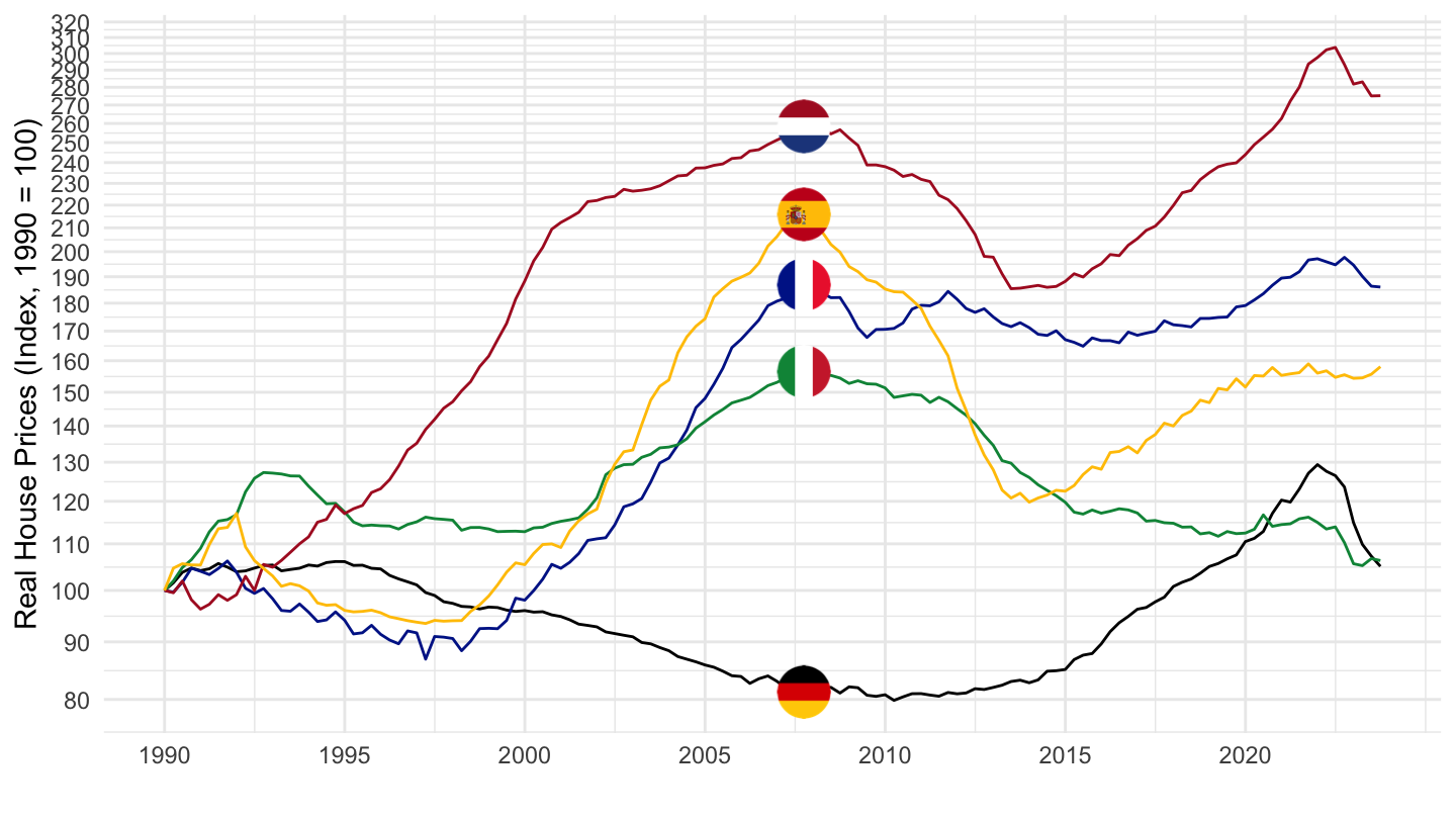
1998-
Code
SELECTED_PP %>%
  filter(iso3c %in% c("DEU", "FRA", "ITA", "ESP", "NLD"),
         FREQ == "Q",
         date >= as.Date("1997-12-31"),
         VALUE == "R",
         UNIT_MEASURE == 628) %>%
  left_join(colors, by = c("Reference area" = "country")) %>%
  mutate(color = ifelse(iso3c == "FRA", color2, color)) %>%
  group_by(iso3c) %>%
  mutate(value = 100*value/value[date == as.Date("1997-12-31")]) %>%
  ggplot(.) + theme_minimal() + xlab("") + ylab("Real House Prices (Index, 1998 = 100)") +
  geom_line(aes(x = date, y = value, color = color)) +
  scale_color_identity() + add_flags +
  scale_x_date(breaks = seq(1900, 2100, 2) %>% paste0("-01-01") %>% as.Date,
               labels = date_format("%Y")) +
  scale_y_log10(breaks = seq(0, 600, 10),
                     labels = dollar_format(a = 1, prefix = "")) +
  theme(legend.position = c(0.8, 0.2),
        legend.title = element_blank())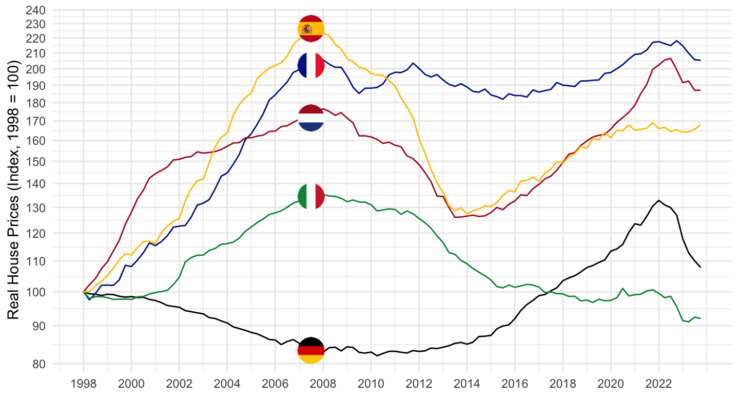
2000-
Code
SELECTED_PP %>%
  filter(iso3c %in% c("DEU", "FRA", "ITA", "ESP", "NLD"),
         FREQ == "Q",
         date >= as.Date("1999-12-31"),
         VALUE == "R",
         UNIT_MEASURE == 628) %>%
  left_join(colors, by = c("Reference area" = "country")) %>%
  mutate(color = ifelse(iso3c == "FRA", color2, color)) %>%
  group_by(iso3c) %>%
  mutate(value = 100*value/value[date == as.Date("1999-12-31")]) %>%
  ggplot(.) + theme_minimal() + xlab("") + ylab("Real House Prices (Index, 2000 = 100)") +
  geom_line(aes(x = date, y = value, color = color)) +
  scale_color_identity() + add_flags +
  scale_x_date(breaks = seq(1900, 2100, 2) %>% paste0("-01-01") %>% as.Date,
               labels = date_format("%Y")) +
  scale_y_log10(breaks = seq(0, 600, 10),
                     labels = dollar_format(a = 1, prefix = "")) +
  theme(legend.position = c(0.8, 0.2),
        legend.title = element_blank())
2020-
Code
SELECTED_PP %>%
  filter(iso3c %in% c("DEU", "FRA", "ITA", "ESP", "NLD"),
         FREQ == "Q",
         date >= as.Date("2019-12-31"),
         VALUE == "R",
         UNIT_MEASURE == 628) %>%
  left_join(colors, by = c("Reference area" = "country")) %>%
  mutate(color = ifelse(iso3c == "FRA", color2, color)) %>%
  group_by(iso3c) %>%
  mutate(value = 100*value/value[date == as.Date("2019-12-31")]) %>%
  mutate(date = zoo::as.yearqtr(OBS_TIME, format = "%Y-Q%q")) %>%
  ggplot(.) + theme_minimal() + xlab("") + ylab("Real House Prices (Index, 2020 = 100)") +
  geom_line(aes(x = date, y = value, color = color)) +
  scale_color_identity() + add_flags +
  scale_y_log10(breaks = seq(0, 600, 5),
                     labels = dollar_format(a = 1, prefix = "")) +
  zoo::scale_x_yearqtr(format = "%YQ%q") +
  theme(legend.position = c(0.8, 0.2),
        legend.title = element_blank(),
        axis.text.x = element_text(angle = 45, vjust = 1, hjust = 1))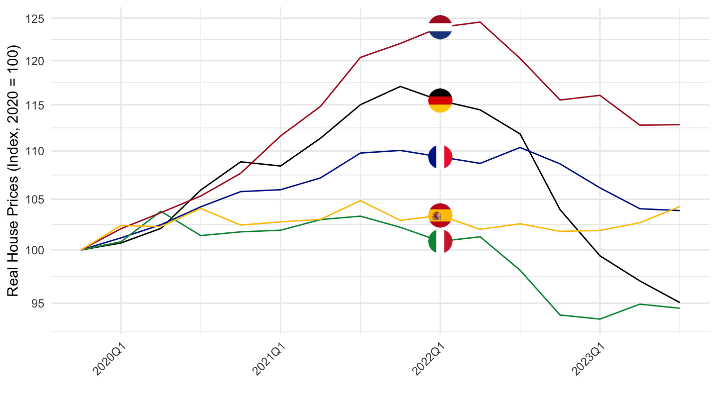
2021Q4-
Code
SELECTED_PP %>%
  filter(iso3c %in% c("DEU", "FRA", "ITA", "ESP", "NLD"),
         FREQ == "Q",
         zoo::as.yearqtr(OBS_TIME, format = "%Y-Q%q") >= zoo::as.yearqtr("2021 Q4"),
         VALUE == "R",
         UNIT_MEASURE == 628) %>%
  mutate(date = zoo::as.yearqtr(OBS_TIME, format = "%Y-Q%q")) %>%
  left_join(colors, by = c("Reference area" = "country")) %>%
  mutate(color = ifelse(iso3c == "FRA", color2, color)) %>%
  group_by(iso3c) %>%
  mutate(value = 100*value/value[date == zoo::as.yearqtr("2021 Q4")]) %>%
  ggplot(.) + theme_minimal() + xlab("") + ylab("Real House Prices (Index, 2020 = 100)") +
  geom_line(aes(x = date, y = value, color = color)) +
  scale_color_identity() + add_flags +
  scale_y_log10(breaks = seq(0, 600, 5),
                     labels = dollar_format(a = 1, prefix = "")) +
  zoo::scale_x_yearqtr(format = "%YQ%q") +
  theme(legend.position = c(0.8, 0.2),
        legend.title = element_blank(),
        axis.text.x = element_text(angle = 45, vjust = 1, hjust = 1))
Germany, France, Italy
All
Code
SELECTED_PP %>%
  filter(iso3c %in% c("DEU", "FRA", "ITA"),
         FREQ == "Q",
         date >= as.Date("1970-03-31"),
         VALUE == "R",
         UNIT_MEASURE == 628) %>%
  left_join(colors, by = c("Reference area" = "country")) %>%
  group_by(iso3c) %>%
  mutate(value = 100*value/value[date == as.Date("1970-03-31")]) %>%
  ggplot(.) + theme_minimal() + xlab("") + ylab("Real House Prices (Index, 2010 = 100)") +
  geom_line(aes(x = date, y = value, color = color)) +
  scale_color_identity() + add_flags +
  scale_x_date(breaks = seq(1900, 2100, 5) %>% paste0("-01-01") %>% as.Date,
               labels = date_format("%Y")) +
  scale_y_log10(breaks = seq(0, 600, 10),
                     labels = dollar_format(a = 1, prefix = "")) +
  theme(legend.position = c(0.8, 0.2),
        legend.title = element_blank())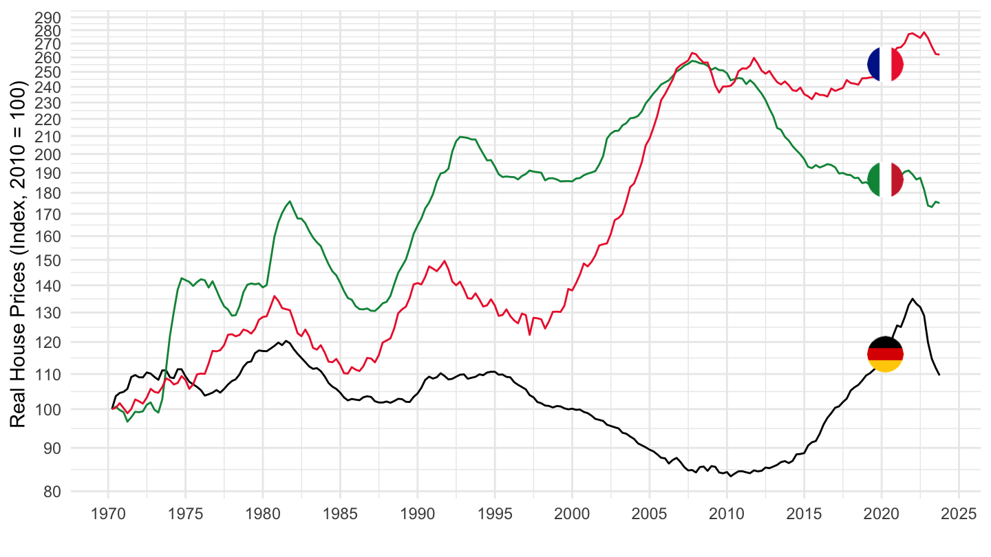
1990-
Code
SELECTED_PP %>%
  filter(iso3c %in% c("DEU", "FRA", "ITA"),
         FREQ == "Q",
         date >= as.Date("1989-12-31"),
         VALUE == "R",
         UNIT_MEASURE == 628) %>%
  left_join(colors, by = c("Reference area" = "country")) %>%
  group_by(iso3c) %>%
  mutate(value = 100*value/value[date == as.Date("1989-12-31")]) %>%
  ggplot(.) + theme_minimal() + xlab("") + ylab("Real House Prices (Index, 1990 = 100)") +
  geom_line(aes(x = date, y = value, color = color)) +
  scale_color_identity() + add_flags +
  scale_x_date(breaks = seq(1900, 2100, 5) %>% paste0("-01-01") %>% as.Date,
               labels = date_format("%Y")) +
  scale_y_log10(breaks = seq(0, 600, 10),
                     labels = dollar_format(a = 1, prefix = "")) +
  theme(legend.position = c(0.8, 0.2),
        legend.title = element_blank())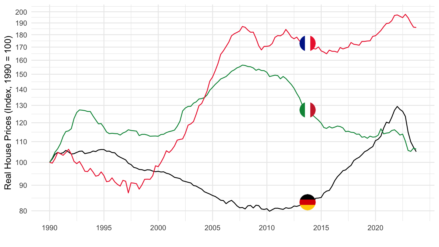
1998-
Code
SELECTED_PP %>%
  filter(iso3c %in% c("DEU", "FRA", "ITA"),
         FREQ == "Q",
         date >= as.Date("1997-12-31"),
         VALUE == "R",
         UNIT_MEASURE == 628) %>%
  left_join(colors, by = c("Reference area" = "country")) %>%
  group_by(iso3c) %>%
  mutate(value = 100*value/value[date == as.Date("1997-12-31")]) %>%
  ggplot(.) + theme_minimal() + xlab("") + ylab("Real House Prices (Index, 1998 = 100)") +
  geom_line(aes(x = date, y = value, color = color)) +
  scale_color_identity() + add_flags +
  scale_x_date(breaks = seq(1900, 2100, 2) %>% paste0("-01-01") %>% as.Date,
               labels = date_format("%Y")) +
  scale_y_log10(breaks = seq(0, 600, 10),
                     labels = dollar_format(a = 1, prefix = "")) +
  theme(legend.position = c(0.8, 0.2),
        legend.title = element_blank())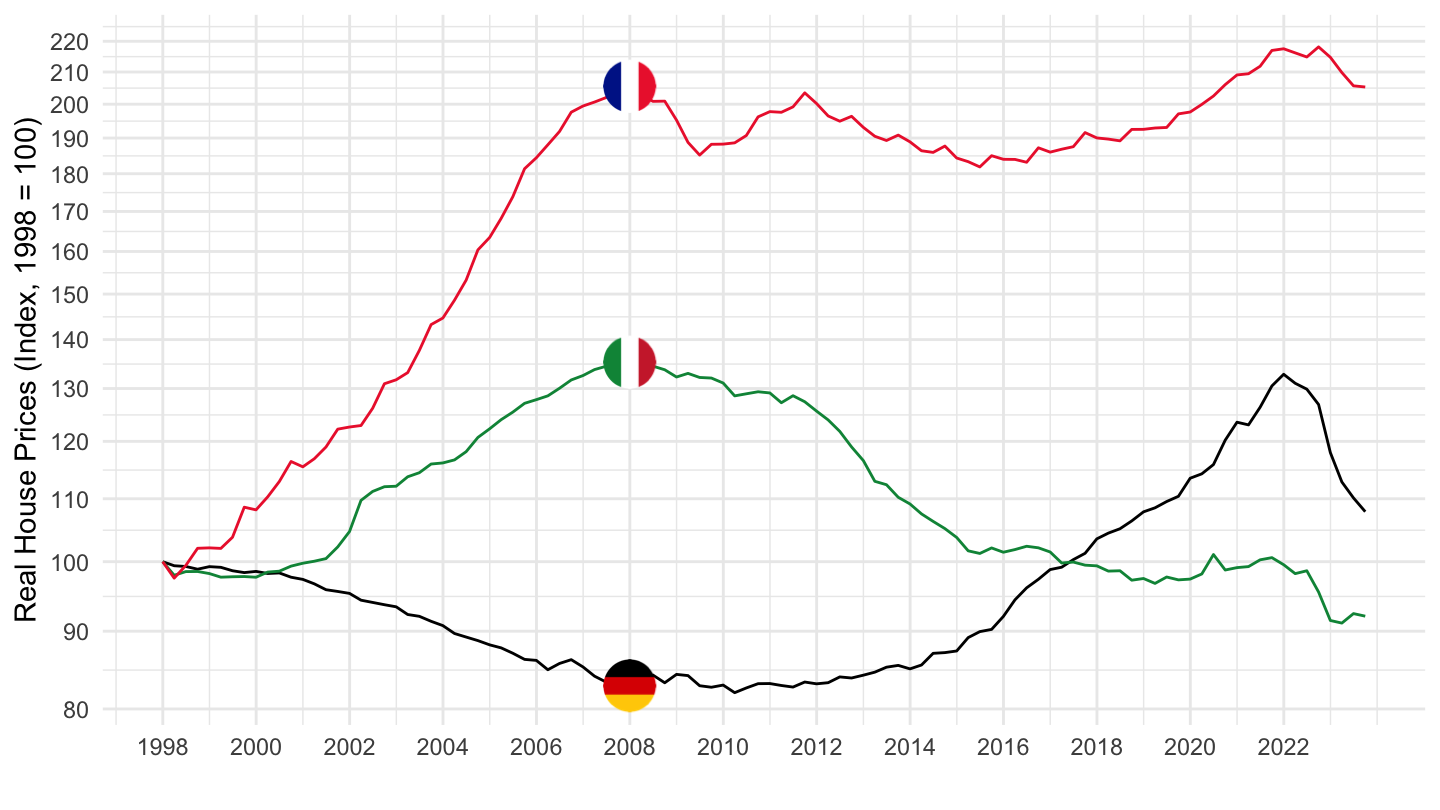
2000-
Code
SELECTED_PP %>%
  filter(iso3c %in% c("DEU", "FRA", "ITA"),
         FREQ == "Q",
         date >= as.Date("1999-12-31"),
         VALUE == "R",
         UNIT_MEASURE == 628) %>%
  left_join(colors, by = c("Reference area" = "country")) %>%
  group_by(iso3c) %>%
  mutate(value = 100*value/value[date == as.Date("1999-12-31")]) %>%
  ggplot(.) + theme_minimal() + xlab("") + ylab("Real House Prices (Index, 2000 = 100)") +
  geom_line(aes(x = date, y = value, color = color)) +
  scale_color_identity() + add_flags +
  scale_x_date(breaks = seq(1900, 2100, 2) %>% paste0("-01-01") %>% as.Date,
               labels = date_format("%Y")) +
  scale_y_log10(breaks = seq(0, 600, 10),
                     labels = dollar_format(a = 1, prefix = "")) +
  theme(legend.position = c(0.8, 0.2),
        legend.title = element_blank())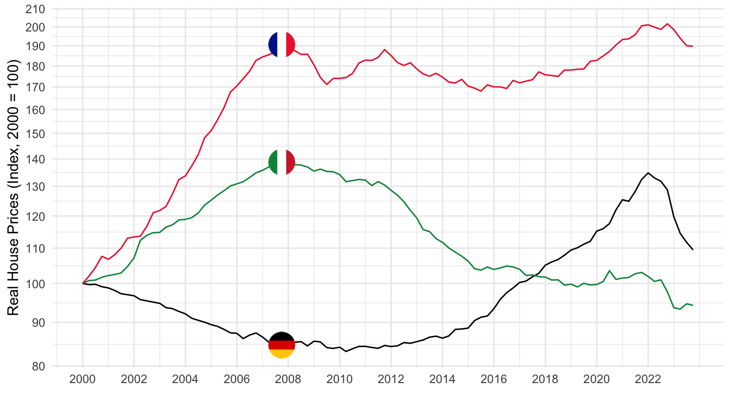
2008-
Code
SELECTED_PP %>%
  filter(iso3c %in% c("DEU", "FRA", "ITA"),
         FREQ == "Q",
         date >= as.Date("2007-12-31"),
         VALUE == "R",
         UNIT_MEASURE == 628) %>%
  left_join(colors, by = c("Reference area" = "country")) %>%
  group_by(iso3c) %>%
  mutate(value = 100*value/value[date == as.Date("2007-12-31")]) %>%
  ggplot(.) + theme_minimal() + xlab("") + ylab("Real House Prices (Index, 2008 = 100)") +
  geom_line(aes(x = date, y = value, color = color)) +
  scale_color_identity() + add_flags +
  scale_x_date(breaks = seq(1900, 2100, 2) %>% paste0("-01-01") %>% as.Date,
               labels = date_format("%Y")) +
  scale_y_log10(breaks = seq(0, 600, 10),
                     labels = dollar_format(a = 1, prefix = "")) +
  theme(legend.position = c(0.8, 0.2),
        legend.title = element_blank())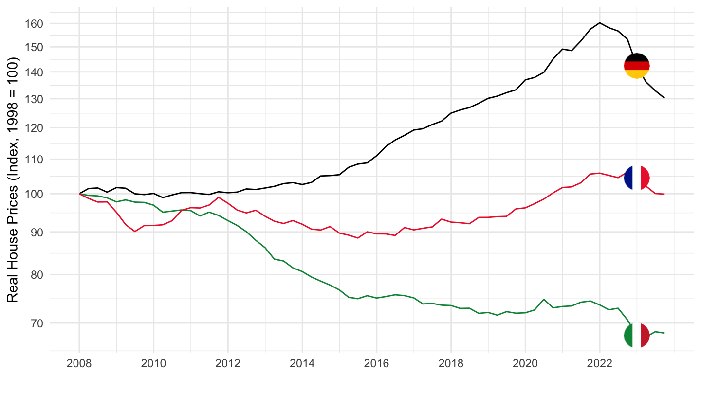
Euro Area, US, France, Germany, United Kingdom
1990-
Code
SELECTED_PP %>%
  filter(iso3c %in% c("DEU", "FRA", "USA", "GBR") | `Reference area` == "Euro area",
         FREQ == "Q",
         date >= as.Date("1990-01-01"),
         VALUE == "R",
         UNIT_MEASURE == 628) %>%
  mutate(`Reference area` = ifelse(`Reference area` == "Euro area", "Europe", `Reference area`)) %>%
  left_join(colors, by = c("Reference area" = "country")) %>%
  group_by(`Reference area`) %>%
  arrange(date) %>%
  mutate(value = 100*value/value[1]) %>%
  ggplot(.) + theme_minimal() + xlab("") + ylab("Real House Prices (Index, 1990 = 100)") +
  geom_line(aes(x = date, y = value, color = color)) +
  scale_color_identity() + add_flags +
  scale_x_date(breaks = seq(1900, 2100, 5) %>% paste0("-01-01") %>% as.Date,
               labels = date_format("%Y")) +
  scale_y_log10(breaks = seq(0, 600, 10),
                     labels = dollar_format(a = 1, prefix = "")) +
  theme(legend.position = c(0.8, 0.2),
        legend.title = element_blank())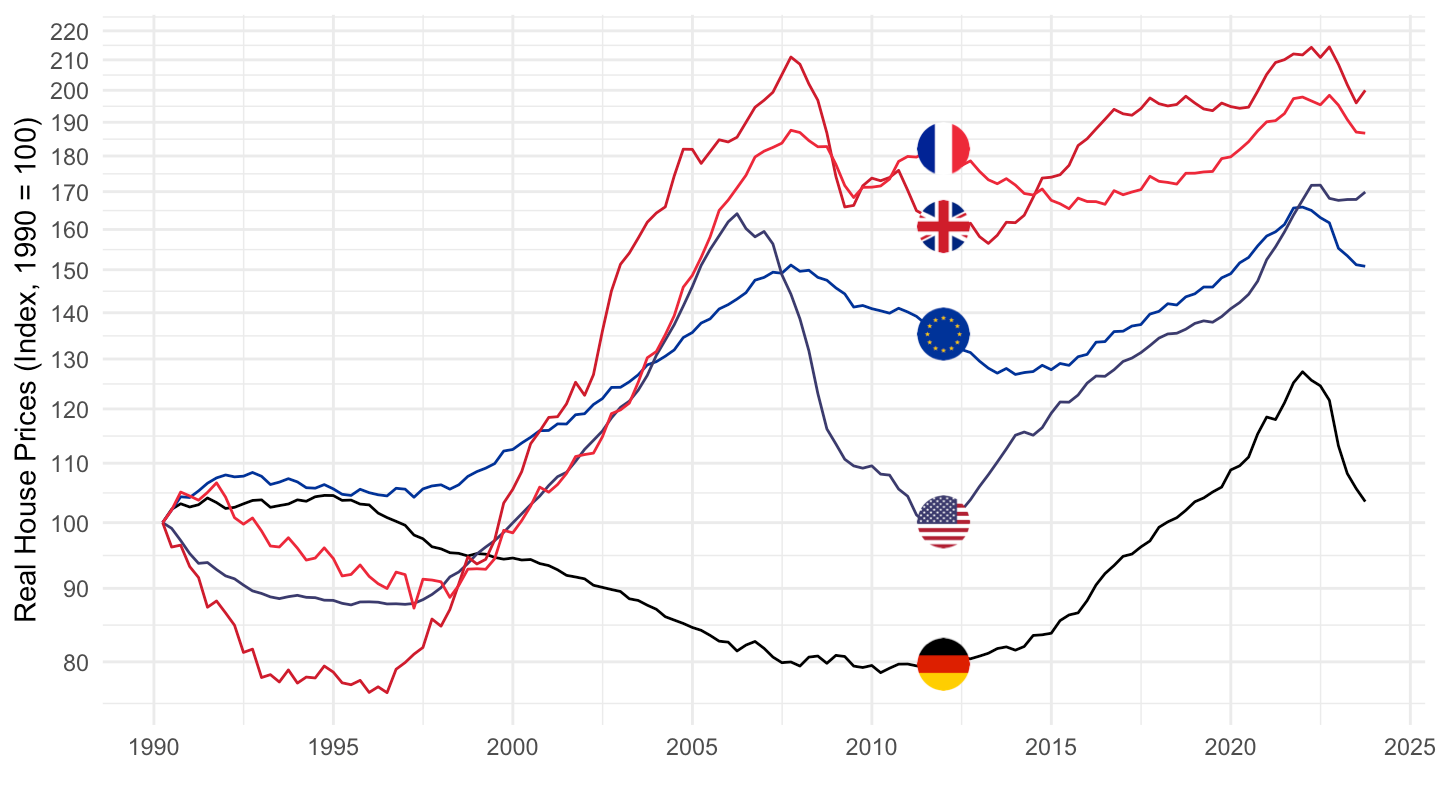
Euro Area, US, France, Germany
All
Code
SELECTED_PP %>%
  filter(iso3c %in% c("DEU", "FRA", "USA") | `Reference area` == "Euro area",
         FREQ == "Q",
         date >= as.Date("1970-01-01"),
         VALUE == "R",
         UNIT_MEASURE == 628) %>%
  mutate(`Reference area` = ifelse(`Reference area` == "Euro area", "Europe", `Reference area`)) %>%
  left_join(colors, by = c("Reference area" = "country")) %>%
  ggplot(.) + theme_minimal() + xlab("") + ylab("Real House Prices (Index, 2010 = 100)") +
  geom_line(aes(x = date, y = value, color = color)) +
  scale_color_identity() + add_flags +
  scale_x_date(breaks = seq(1900, 2100, 5) %>% paste0("-01-01") %>% as.Date,
               labels = date_format("%Y")) +
  scale_y_log10(breaks = seq(0, 600, 10),
                     labels = dollar_format(a = 1, prefix = "")) +
  theme(legend.position = c(0.8, 0.2),
        legend.title = element_blank())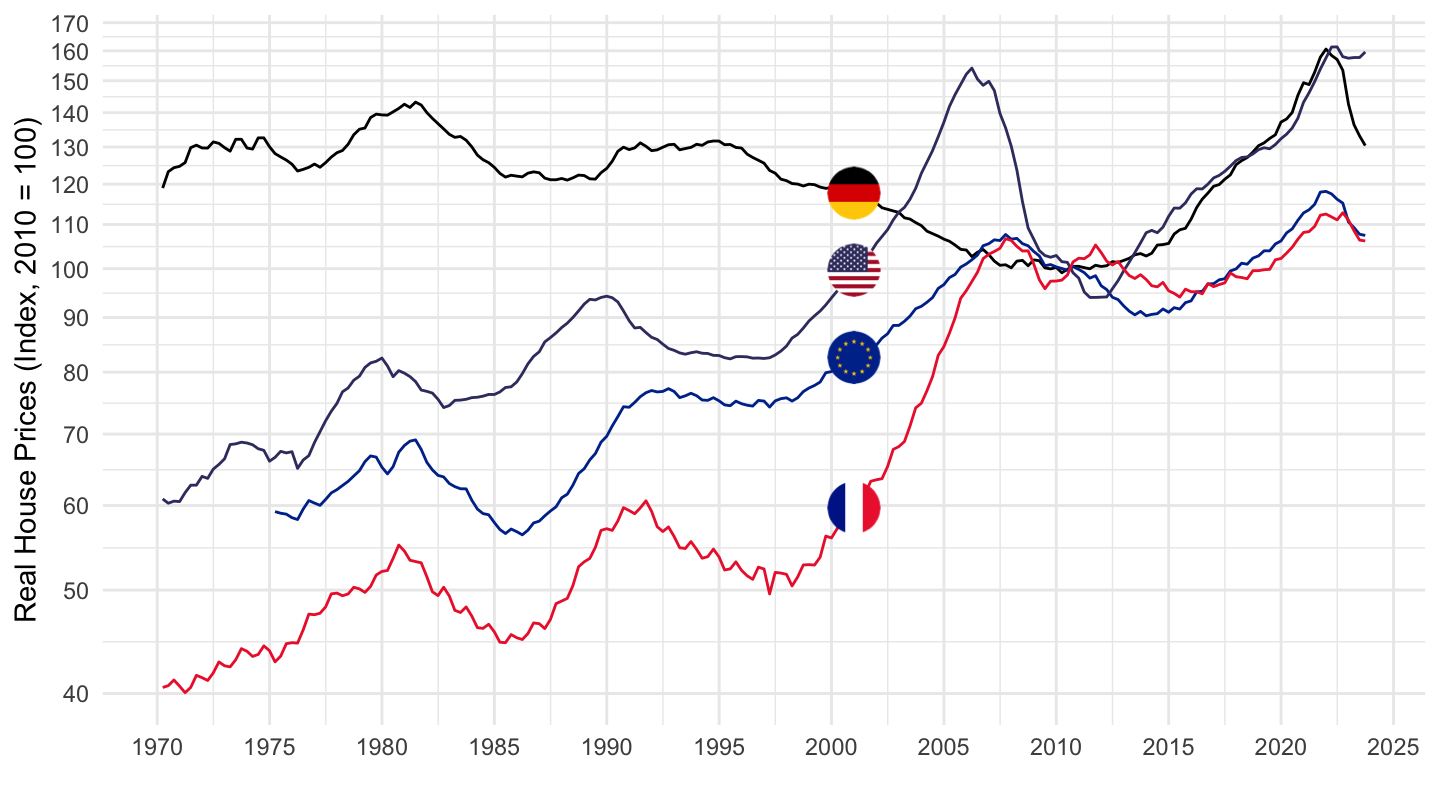
1975
Code
SELECTED_PP %>%
  filter(iso3c %in% c("DEU", "FRA", "USA") | `Reference area` == "Euro area",
         FREQ == "Q",
         date >= as.Date("1975-01-01"),
         VALUE == "R",
         UNIT_MEASURE == 628) %>%
  mutate(`Reference area` = ifelse(`Reference area` == "Euro area", "Europe", `Reference area`)) %>%
  left_join(colors, by = c("Reference area" = "country")) %>%
  group_by(`Reference area`) %>%
  arrange(date) %>%
  mutate(value = 100*value/value[1]) %>%
  ggplot(.) + theme_minimal() + xlab("") + ylab("Real House Prices (Index, 1975 = 100)") +
  geom_line(aes(x = date, y = value, color = color)) +
  scale_color_identity() + add_flags +
  scale_x_date(breaks = seq(1900, 2100, 5) %>% paste0("-01-01") %>% as.Date,
               labels = date_format("%Y")) +
  scale_y_log10(breaks = seq(0, 600, 10),
                     labels = dollar_format(a = 1, prefix = "")) +
  theme(legend.position = c(0.8, 0.2),
        legend.title = element_blank())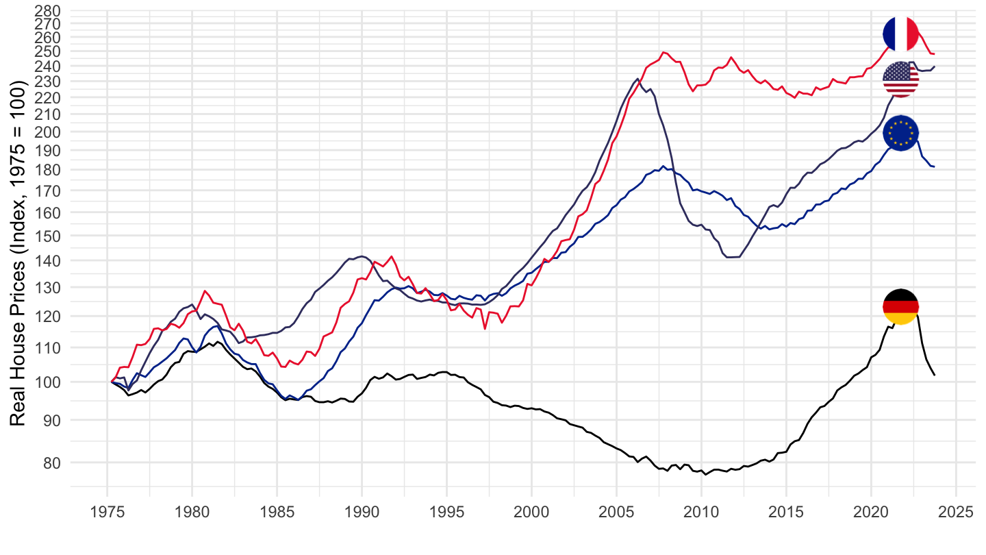
1990-
Code
SELECTED_PP %>%
  filter(iso3c %in% c("DEU", "FRA", "USA") | `Reference area` == "Euro area",
         FREQ == "Q",
         date >= as.Date("1990-01-01"),
         VALUE == "R",
         UNIT_MEASURE == 628) %>%
  mutate(`Reference area` = ifelse(`Reference area` == "Euro area", "Europe", `Reference area`)) %>%
  left_join(colors, by = c("Reference area" = "country")) %>%
  group_by(`Reference area`) %>%
  arrange(date) %>%
  mutate(value = 100*value/value[1]) %>%
  ggplot(.) + theme_minimal() + xlab("") + ylab("Real House Prices (Index, 1990 = 100)") +
  geom_line(aes(x = date, y = value, color = color)) +
  scale_color_identity() + add_flags +
  scale_x_date(breaks = seq(1900, 2100, 5) %>% paste0("-01-01") %>% as.Date,
               labels = date_format("%Y")) +
  scale_y_log10(breaks = seq(0, 600, 10),
                     labels = dollar_format(a = 1, prefix = "")) +
  theme(legend.position = c(0.8, 0.2),
        legend.title = element_blank())
1998-
Code
SELECTED_PP %>%
  filter(iso3c %in% c("DEU", "FRA", "USA") | `Reference area` == "Euro area",
         FREQ == "Q",
         date >= as.Date("1998-01-01"),
         VALUE == "R",
         UNIT_MEASURE == 628) %>%
  mutate(`Reference area` = ifelse(`Reference area` == "Euro area", "Europe", `Reference area`)) %>%
  left_join(colors, by = c("Reference area" = "country")) %>%
  group_by(`Reference area`) %>%
  arrange(date) %>%
  mutate(value = 100*value/value[1]) %>%
  ggplot(.) + theme_minimal() + xlab("") + ylab("Real House Prices (Index, 1998 = 100)") +
  geom_line(aes(x = date, y = value, color = color)) +
  scale_color_identity() + add_flags +
  scale_x_date(breaks = seq(1900, 2100, 2) %>% paste0("-01-01") %>% as.Date,
               labels = date_format("%Y")) +
  scale_y_log10(breaks = seq(0, 600, 10),
                     labels = dollar_format(a = 1, prefix = "")) +
  theme(legend.position = c(0.8, 0.2),
        legend.title = element_blank())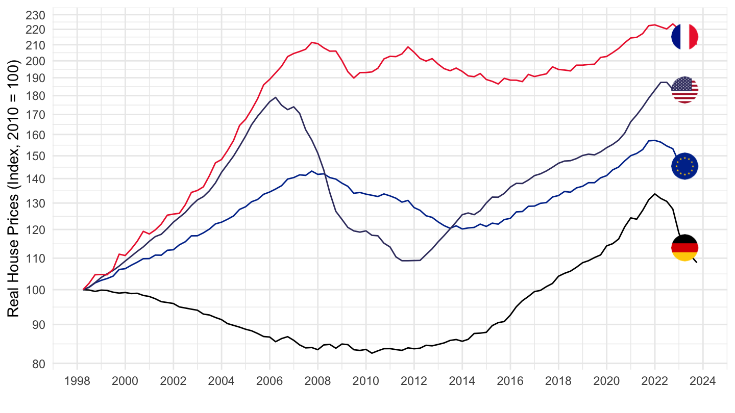
Germany, France, Italy, Japan, United States
All
Code
SELECTED_PP %>%
  filter(iso3c %in% c("DEU", "FRA", "ITA", "JPN", "USA"),
         FREQ == "Q",
         date >= as.Date("1970-01-01"),
         VALUE == "R",
         UNIT_MEASURE == 628) %>%
  left_join(colors, by = c("Reference area" = "country")) %>%
  mutate(color = ifelse(iso3c == "NLD", color2, color)) %>%
  ggplot(.) + theme_minimal() + xlab("") + ylab("Real House Prices (Index, 2010 = 100)") +
  geom_line(aes(x = date, y = value, color = color)) +
  scale_color_identity() + add_flags +
  scale_x_date(breaks = seq(1900, 2100, 5) %>% paste0("-01-01") %>% as.Date,
               labels = date_format("%Y")) +
  scale_y_log10(breaks = seq(0, 600, 10),
                     labels = dollar_format(a = 1, prefix = "")) +
  theme(legend.position = c(0.8, 0.2),
        legend.title = element_blank())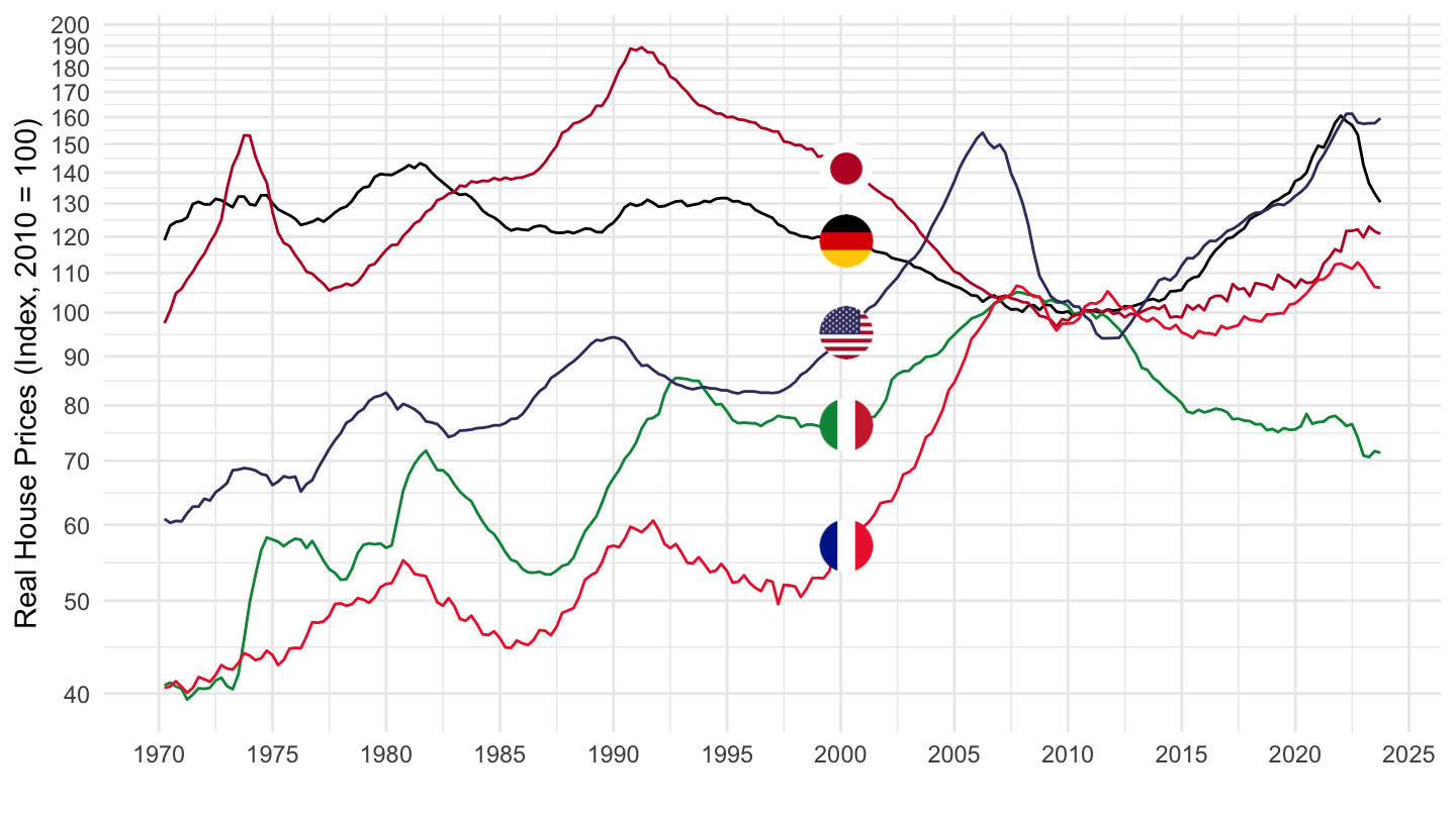
1990-
Code
SELECTED_PP %>%
  filter(iso3c %in% c("DEU", "FRA", "ITA", "JPN", "USA", "ESP"),
         FREQ == "Q",
         date >= as.Date("1990-01-01"),
         VALUE == "R",
         UNIT_MEASURE == 628) %>%
  left_join(colors, by = c("Reference area" = "country")) %>%
  mutate(color = ifelse(iso3c == "NLD", color2, color)) %>%
  group_by(`Reference area`) %>%
  arrange(date) %>%
  mutate(value = 100*value/value[1]) %>%
  ggplot(.) + theme_minimal() + xlab("") + ylab("Real House Prices (Index, 1990 = 100)") +
  geom_line(aes(x = date, y = value, color = color)) +
  scale_color_identity() + add_flags +
  scale_x_date(breaks = seq(1900, 2100, 5) %>% paste0("-01-01") %>% as.Date,
               labels = date_format("%Y")) +
  scale_y_log10(breaks = seq(0, 600, 10),
                     labels = dollar_format(a = 1, prefix = "")) +
  theme(legend.position = c(0.8, 0.2),
        legend.title = element_blank())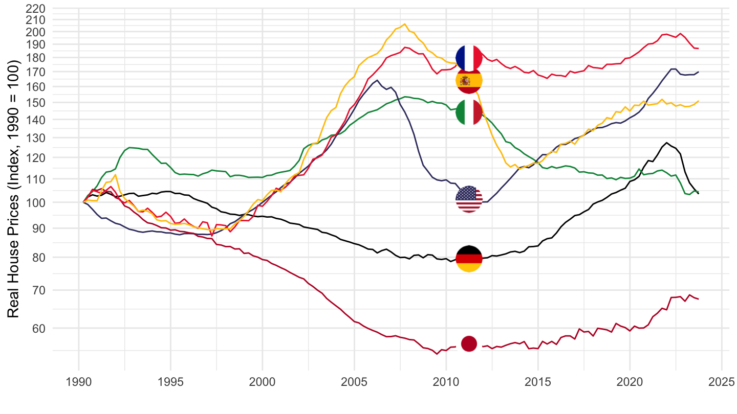
1998-
Code
SELECTED_PP %>%
  filter(iso3c %in% c("DEU", "FRA", "ITA", "JPN", "USA", "ESP"),
         FREQ == "Q",
         date >= as.Date("1998-01-01"),
         VALUE == "R",
         UNIT_MEASURE == 628) %>%
  left_join(colors, by = c("Reference area" = "country")) %>%
  mutate(color = ifelse(iso3c == "NLD", color2, color)) %>%
  group_by(`Reference area`) %>%
  arrange(date) %>%
  mutate(value = 100*value/value[1]) %>%
  ggplot(.) + theme_minimal() + xlab("") + ylab("Real House Prices (Index, 1998 = 100)") +
  geom_line(aes(x = date, y = value, color = color)) +
  scale_color_identity() + add_flags +
  scale_x_date(breaks = seq(1900, 2100, 2) %>% paste0("-01-01") %>% as.Date,
               labels = date_format("%Y")) +
  scale_y_log10(breaks = seq(0, 600, 10),
                     labels = dollar_format(a = 1, prefix = "")) +
  theme(legend.position = c(0.8, 0.2),
        legend.title = element_blank())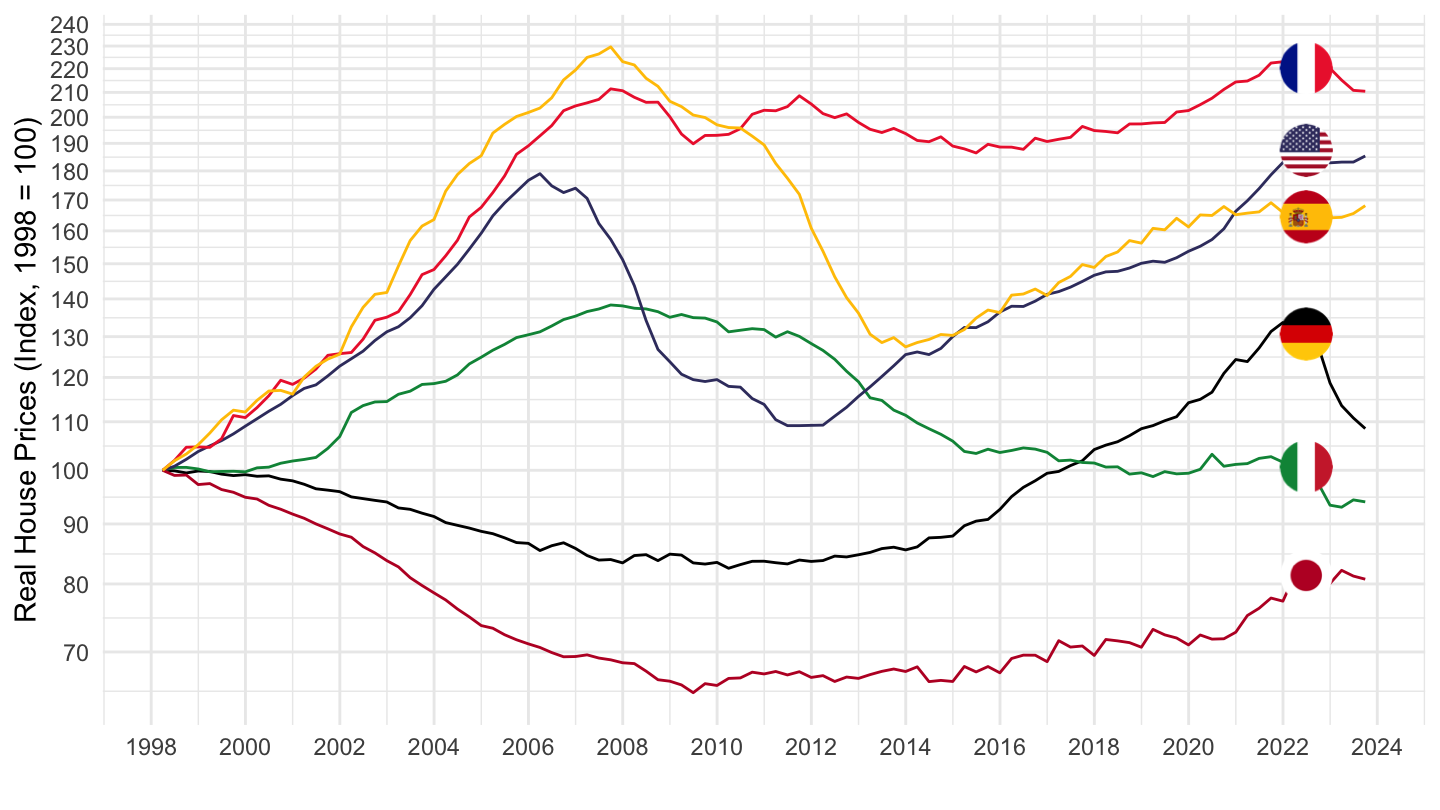
2000-
Code
SELECTED_PP %>%
  filter(iso3c %in% c("DEU", "FRA", "ITA", "JPN", "USA", "ESP"),
         FREQ == "Q",
         date >= as.Date("2000-01-01"),
         VALUE == "R",
         UNIT_MEASURE == 628) %>%
  left_join(colors, by = c("Reference area" = "country")) %>%
  mutate(color = ifelse(iso3c == "NLD", color2, color)) %>%
  group_by(`Reference area`) %>%
  arrange(date) %>%
  mutate(value = 100*value/value[1]) %>%
  ggplot(.) + theme_minimal() + xlab("") + ylab("Real House Prices (Index, 2000 = 100)") +
  geom_line(aes(x = date, y = value, color = color)) +
  scale_color_identity() + add_flags +
  scale_x_date(breaks = seq(1900, 2100, 2) %>% paste0("-01-01") %>% as.Date,
               labels = date_format("%Y")) +
  scale_y_log10(breaks = seq(0, 600, 10),
                     labels = dollar_format(a = 1, prefix = "")) +
  theme(legend.position = c(0.8, 0.2),
        legend.title = element_blank())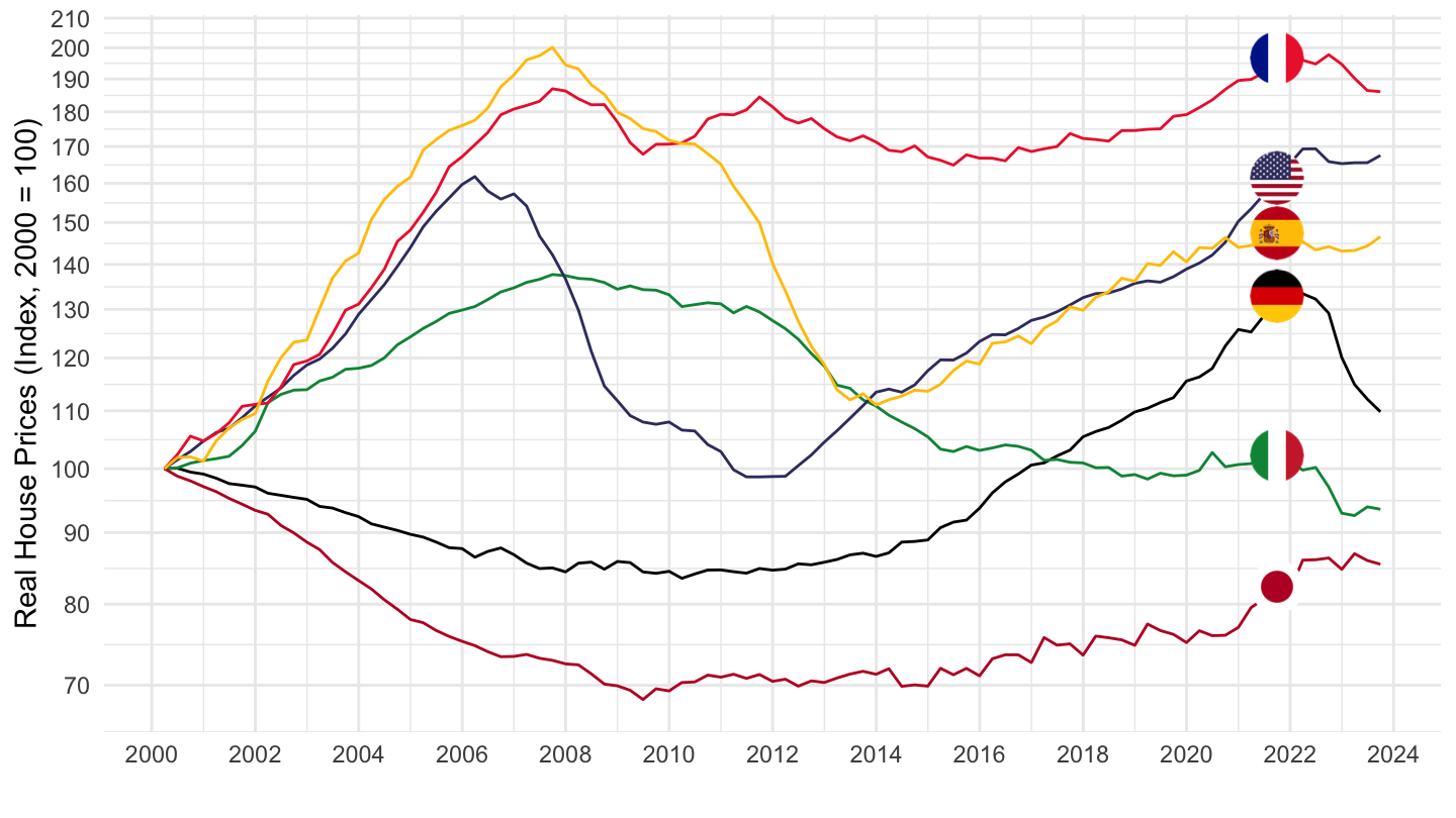
Germany, France, Italy, Spain, Netherlands
Code
SELECTED_PP %>%
  filter(iso3c %in% c("DEU", "FRA", "ITA", "ESP", "NLD"),
         FREQ == "Q",
         date >= as.Date("1970-01-01"),
         VALUE == "R",
         UNIT_MEASURE == 628) %>%
  left_join(colors, by = c("Reference area" = "country")) %>%
  mutate(color = ifelse(iso3c == "NLD", color2, color)) %>%
  ggplot(.) + theme_minimal() + xlab("") + ylab("Real House Prices (Index, 2010 = 100)") +
  geom_line(aes(x = date, y = value, color = color)) +
  scale_color_identity() + add_flags +
  scale_x_date(breaks = seq(1900, 2100, 5) %>% paste0("-01-01") %>% as.Date,
               labels = date_format("%Y")) +
  scale_y_log10(breaks = seq(0, 600, 10),
                     labels = dollar_format(a = 1, prefix = "")) +
  theme(legend.position = c(0.8, 0.2),
        legend.title = element_blank())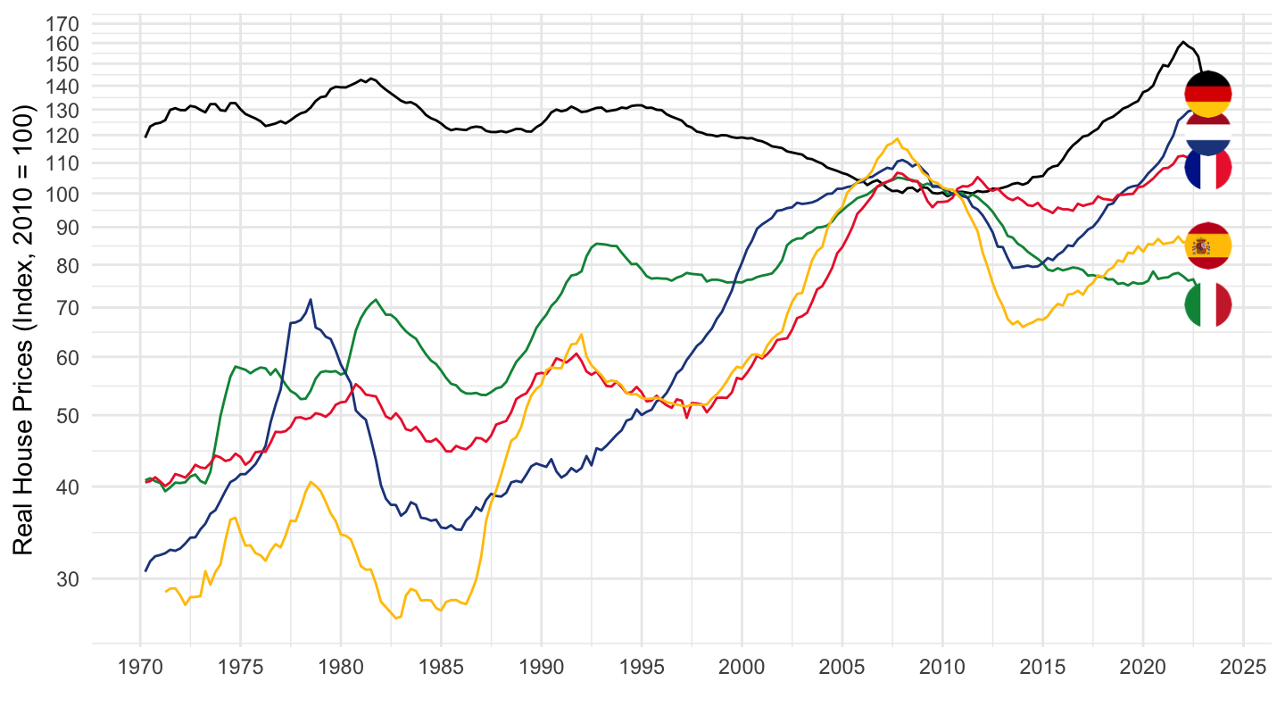
Germany, France, Sweden, Japan
All
Code
SELECTED_PP %>%
  filter(iso3c %in% c("DEU", "FRA", "SWE", "JPN"),
         FREQ == "Q",
         date >= as.Date("1970-01-01"),
         VALUE == "R",
         UNIT_MEASURE == 628) %>%
  left_join(colors, by = c("Reference area" = "country")) %>%
  ggplot(.) + theme_minimal() + xlab("") + ylab("Real House Prices (Index, 2010 = 100)") +
  geom_line(aes(x = date, y = value, color = color)) +
  scale_color_identity() + add_flags +
  scale_x_date(breaks = seq(1900, 2100, 5) %>% paste0("-01-01") %>% as.Date,
               labels = date_format("%Y")) +
  scale_y_log10(breaks = seq(0, 600, 10),
                     labels = dollar_format(a = 1, prefix = "")) +
  theme(legend.position = c(0.8, 0.2),
        legend.title = element_blank())
1998-
Code
SELECTED_PP %>%
  filter(iso3c %in% c("DEU", "FRA", "SWE", "JPN"),
         FREQ == "Q",
         date >= as.Date("1997-12-31"),
         VALUE == "R",
         UNIT_MEASURE == 628) %>%
  left_join(colors, by = c("Reference area" = "country")) %>%
  group_by(`Reference area`) %>%
  mutate(value = 100*value/value[date == as.Date("1997-12-31")]) %>%
  ggplot(.) + theme_minimal() + xlab("") + ylab("Real House Prices (Index, 1998 = 100)") +
  geom_line(aes(x = date, y = value, color = color)) +
  scale_color_identity() + add_flags +
  scale_x_date(breaks = seq(1900, 2100, 2) %>% paste0("-01-01") %>% as.Date,
               labels = date_format("%Y")) +
  scale_y_log10(breaks = seq(0, 600, 10),
                     labels = dollar_format(a = 1, prefix = "")) +
  theme(legend.position = c(0.8, 0.2),
        legend.title = element_blank())
Germany, France, Sweden, Japan, Spain, US, Switzerland
All
Code
SELECTED_PP %>%
  filter(iso3c %in% c("DEU", "FRA", "SWE", "JPN", "ESP", "ITA", "USA", "CHE"),
         FREQ == "Q",
         VALUE == "R",
         date >= as.Date("1972-12-31"),
         UNIT_MEASURE == 628) %>%
  left_join(colors, by = c("Reference area" = "country")) %>%
  group_by(`Reference area`) %>%
  mutate(value = 100*value/value[date == as.Date("1972-12-31")]) %>%
  ggplot(.) + theme_minimal() + xlab("") + ylab("Real House Prices (Index, 1998 = 100)") +
  geom_line(aes(x = date, y = value, color = color)) +
  scale_color_identity() + add_flags +
  scale_x_date(breaks = seq(1900, 2100, 5) %>% paste0("-01-01") %>% as.Date,
               labels = date_format("%Y")) +
  scale_y_log10(breaks = seq(0, 600, 10),
                     labels = dollar_format(a = 1, prefix = "")) +
  theme(legend.position = c(0.8, 0.2),
        legend.title = element_blank())
1998-
Code
SELECTED_PP %>%
  filter(iso3c %in% c("DEU", "FRA", "SWE", "JPN", "ESP", "ITA", "USA", "CHE"),
         FREQ == "Q",
         date >= as.Date("1997-12-31"),
         VALUE == "R",
         UNIT_MEASURE == 628) %>%
  left_join(colors, by = c("Reference area" = "country")) %>%
  group_by(`Reference area`) %>%
  mutate(value = 100*value/value[date == as.Date("1997-12-31")]) %>%
  ggplot(.) + theme_minimal() + xlab("") + ylab("Real House Prices (Index, 1998 = 100)") +
  geom_line(aes(x = date, y = value, color = color)) +
  scale_color_identity() + add_flags +
  scale_x_date(breaks = seq(1900, 2100, 2) %>% paste0("-01-01") %>% as.Date,
               labels = date_format("%Y")) +
  scale_y_log10(breaks = seq(0, 600, 10),
                     labels = dollar_format(a = 1, prefix = "")) +
  theme(legend.position = c(0.8, 0.2),
        legend.title = element_blank())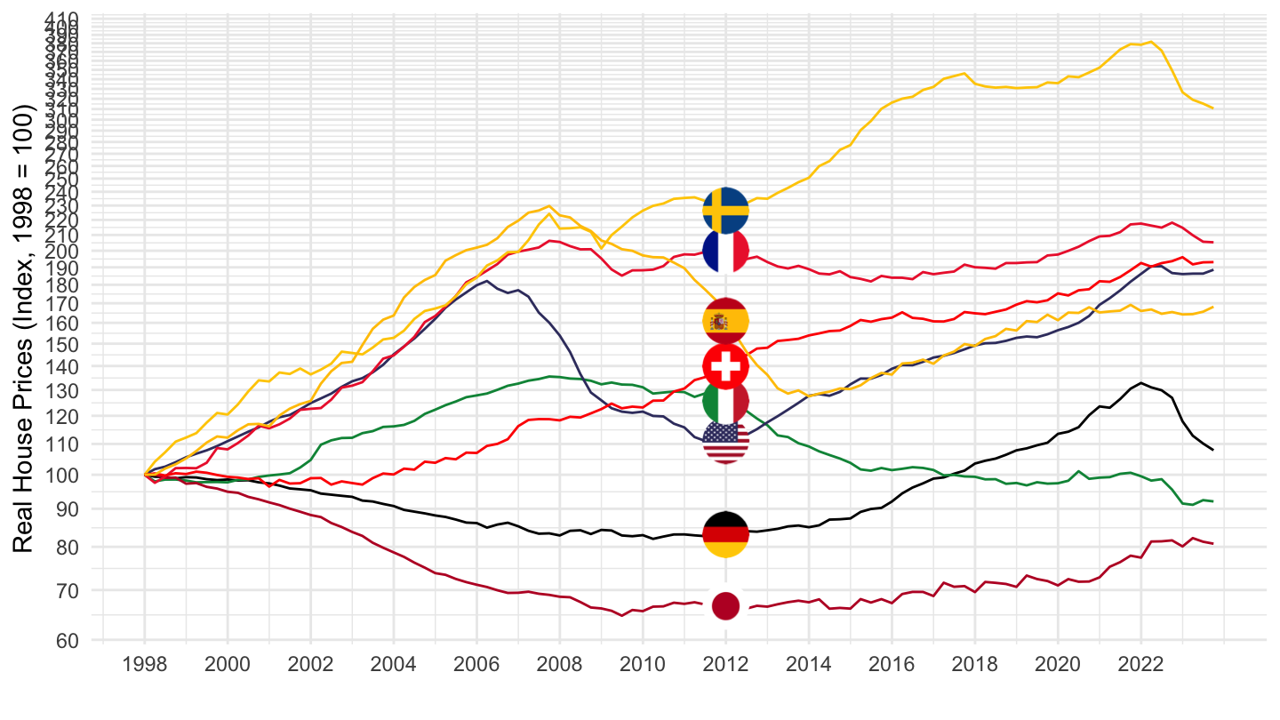
Denmark, Germany, Switzerland
Code
SELECTED_PP %>%
  filter(iso3c %in% c("DEU", "DNK", "CHE"),
         FREQ == "Q",
         date >= as.Date("1970-01-01"),
         VALUE == "R",
         UNIT_MEASURE == 628) %>%
  left_join(colors, by = c("Reference area" = "country")) %>%
  ggplot(.) + theme_minimal() + xlab("") + ylab("Real House Prices (Index, 2010 = 100)") +
  geom_line(aes(x = date, y = value, color = color)) +
  scale_color_identity() + add_flags +
  scale_x_date(breaks = seq(1900, 2100, 5) %>% paste0("-01-01") %>% as.Date,
               labels = date_format("%Y")) +
  scale_y_log10(breaks = seq(0, 600, 10),
                     labels = dollar_format(a = 1, prefix = "")) +
  theme(legend.position = c(0.8, 0.2),
        legend.title = element_blank())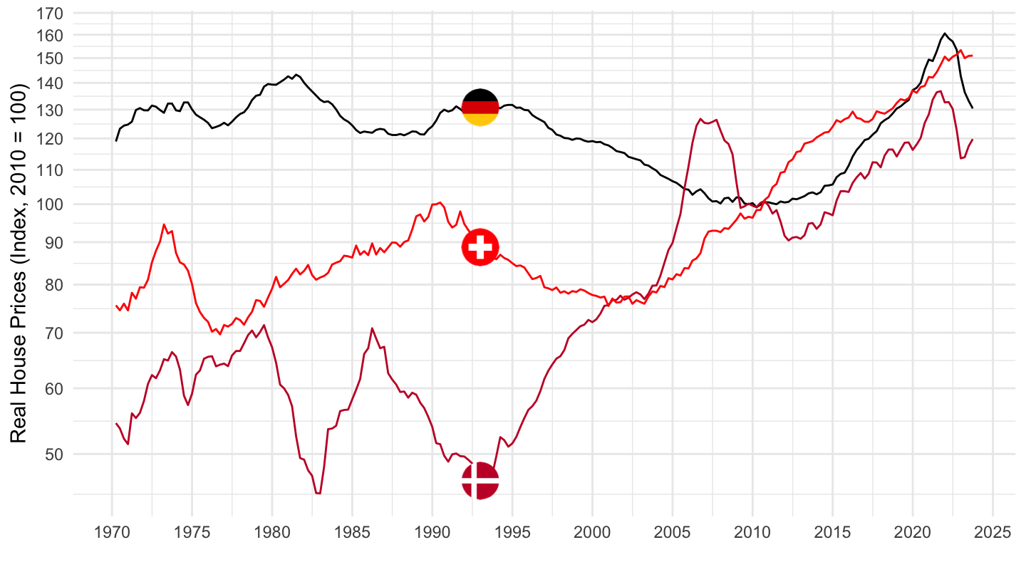
Nominal House Prices
Germany, France, US, Europe
1975
Code
SELECTED_PP %>%
  filter(iso3c %in% c("DEU", "FRA", "USA") | `Reference area` == "Euro area",
         FREQ == "Q",
         date >= as.Date("1975-01-01"),
         VALUE == "N",
         UNIT_MEASURE == 628) %>%
  mutate(`Reference area` = ifelse(`Reference area` == "Euro area", "Europe", `Reference area`)) %>%
  left_join(colors, by = c("Reference area" = "country")) %>%
  group_by(`Reference area`) %>%
  arrange(date) %>%
  mutate(value = 100*value/value[1]) %>%
  ggplot(.) + theme_minimal() + xlab("") + ylab("Nominal House Prices (Index, 1975 = 100)") +
  geom_line(aes(x = date, y = value, color = color)) +
  scale_color_identity() + add_flags +
  scale_x_date(breaks = seq(1900, 2100, 5) %>% paste0("-01-01") %>% as.Date,
               labels = date_format("%Y")) +
  scale_y_log10(breaks = seq(0, 2000, 100),
                     labels = dollar_format(a = 1, prefix = "")) +
  theme(legend.position = c(0.8, 0.2),
        legend.title = element_blank())
2007-
Code
SELECTED_PP %>%
  filter(iso3c %in% c("DEU", "FRA", "USA") | `Reference area` == "Euro area",
         FREQ == "Q",
         date >= as.Date("2007-01-01"),
         VALUE == "N",
         UNIT_MEASURE == 628) %>%
  mutate(`Reference area` = ifelse(`Reference area` == "Euro area", "Europe", `Reference area`)) %>%
  left_join(colors, by = c("Reference area" = "country")) %>%
  group_by(`Reference area`) %>%
  arrange(date) %>%
  mutate(value = 100*value/value[1]) %>%
  ggplot(.) + theme_minimal() + xlab("") + ylab("Nominal House Prices (Index, 2007 = 100)") +
  geom_line(aes(x = date, y = value, color = color)) +
  scale_color_identity() + add_flags +
  scale_x_date(breaks = seq(2007, 2100, 2) %>% paste0("-01-01") %>% as.Date,
               labels = date_format("%Y")) +
  scale_y_log10(breaks = seq(0, 2000, 10),
                     labels = dollar_format(a = 1, prefix = "")) +
  theme(legend.position = c(0.8, 0.2),
        legend.title = element_blank())
France, Italy, Spain, United States
1990-
Code
SELECTED_PP %>%
  filter(iso3c %in% c("FRA", "ESP", "NLD", "USA"),
         FREQ == "Q",
         date >= as.Date("1989-12-31"),
         VALUE == "N",
         UNIT_MEASURE == 628) %>%
  left_join(colors, by = c("Reference area" = "country")) %>%
  mutate(color = ifelse(iso3c == "FRA", color2, color)) %>%
  group_by(iso3c) %>%
  mutate(value = 100*value/value[date == as.Date("1989-12-31")]) %>%
  ggplot(.) + theme_minimal() + xlab("") + ylab("Nominal House Prices (Index, 1990 = 100)") +
  geom_line(aes(x = date, y = value, color = color)) +
  scale_color_identity() + add_flags +
  scale_x_date(breaks = seq(1900, 2100, 5) %>% paste0("-01-01") %>% as.Date,
               labels = date_format("%Y")) +
  scale_y_log10(breaks = seq(0, 600, 10),
                     labels = dollar_format(a = 1, prefix = "")) +
  theme(legend.position = c(0.8, 0.2),
        legend.title = element_blank())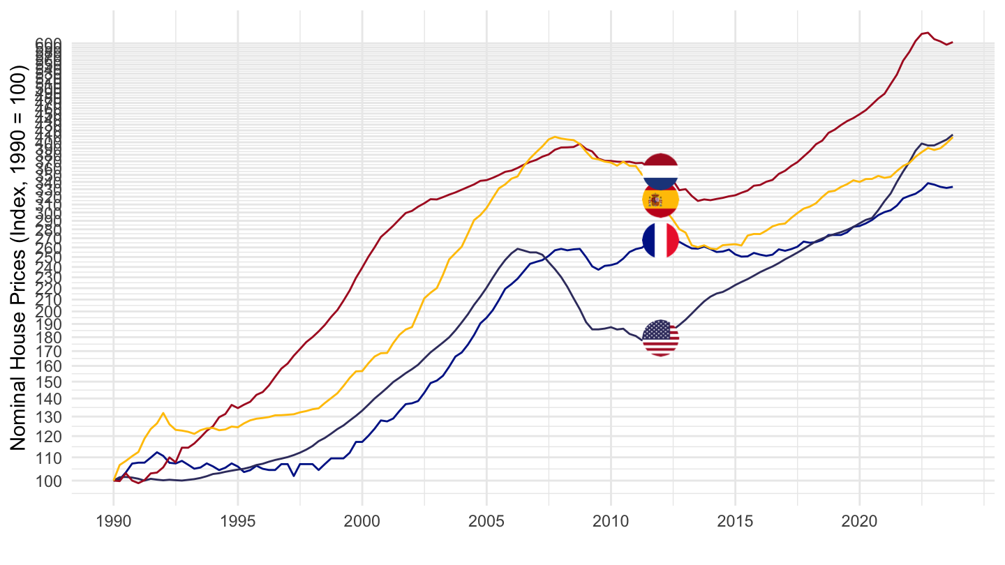
2000-
Code
SELECTED_PP %>%
  filter(iso3c %in% c("FRA", "ESP", "NLD", "USA"),
         FREQ == "Q",
         date >= as.Date("1999-12-31"),
         VALUE == "N",
         UNIT_MEASURE == 628) %>%
  left_join(colors, by = c("Reference area" = "country")) %>%
  mutate(color = ifelse(iso3c == "FRA", color2, color)) %>%
  group_by(iso3c) %>%
  mutate(value = 100*value/value[date == as.Date("1999-12-31")]) %>%
  ggplot(.) + theme_minimal() + xlab("") + ylab("Nominal House Prices (Index, 2000 = 100)") +
  geom_line(aes(x = date, y = value, color = color)) +
  scale_color_identity() + add_flags +
  scale_x_date(breaks = seq(1900, 2100, 2) %>% paste0("-01-01") %>% as.Date,
               labels = date_format("%Y")) +
  scale_y_log10(breaks = seq(0, 600, 10),
                     labels = dollar_format(a = 1, prefix = "")) +
  theme(legend.position = c(0.8, 0.2),
        legend.title = element_blank())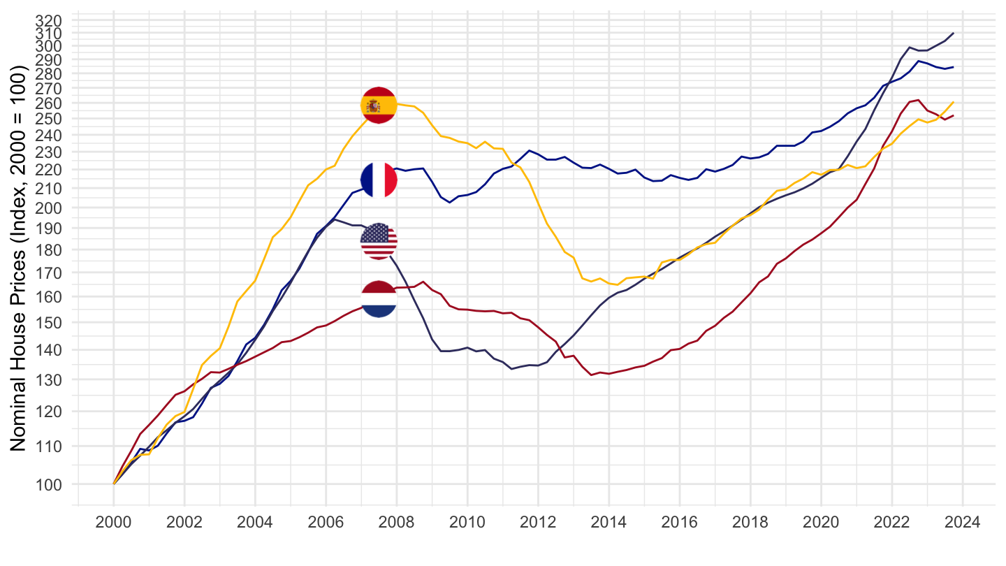
Germany, France, Italy, Spain, Nertherlands
1990-
Code
SELECTED_PP %>%
  filter(iso3c %in% c("DEU", "FRA", "ITA", "ESP", "NLD"),
         FREQ == "Q",
         date >= as.Date("1989-12-31"),
         VALUE == "N",
         UNIT_MEASURE == 628) %>%
  left_join(colors, by = c("Reference area" = "country")) %>%
  mutate(color = ifelse(iso3c == "FRA", color2, color)) %>%
  group_by(iso3c) %>%
  mutate(value = 100*value/value[date == as.Date("1989-12-31")]) %>%
  ggplot(.) + theme_minimal() + xlab("") + ylab("Nominal House Prices (Index, 1990 = 100)") +
  geom_line(aes(x = date, y = value, color = color)) +
  scale_color_identity() + add_flags +
  scale_x_date(breaks = seq(1900, 2100, 5) %>% paste0("-01-01") %>% as.Date,
               labels = date_format("%Y")) +
  scale_y_log10(breaks = seq(0, 600, 10),
                     labels = dollar_format(a = 1, prefix = "")) +
  theme(legend.position = c(0.8, 0.2),
        legend.title = element_blank())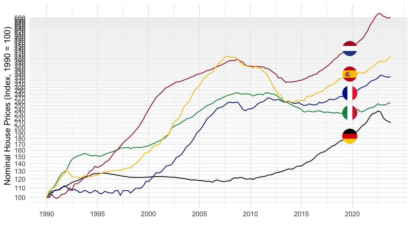
2000-
Code
SELECTED_PP %>%
  filter(iso3c %in% c("DEU", "FRA", "ITA", "ESP", "NLD", "USA"),
         FREQ == "Q",
         date >= as.Date("1999-12-31"),
         VALUE == "N",
         UNIT_MEASURE == 628) %>%
  left_join(colors, by = c("Reference area" = "country")) %>%
  mutate(color = ifelse(iso3c == "FRA", color2, color)) %>%
  group_by(iso3c) %>%
  mutate(value = 100*value/value[date == as.Date("1999-12-31")]) %>%
  ggplot(.) + theme_minimal() + xlab("") + ylab("Nominal House Prices (Index, 1990 = 100)") +
  geom_line(aes(x = date, y = value, color = color)) +
  scale_color_identity() + add_flags +
  scale_x_date(breaks = seq(1900, 2100, 2) %>% paste0("-01-01") %>% as.Date,
               labels = date_format("%Y")) +
  scale_y_log10(breaks = seq(0, 600, 10),
                     labels = dollar_format(a = 1, prefix = "")) +
  theme(legend.position = c(0.8, 0.2),
        legend.title = element_blank())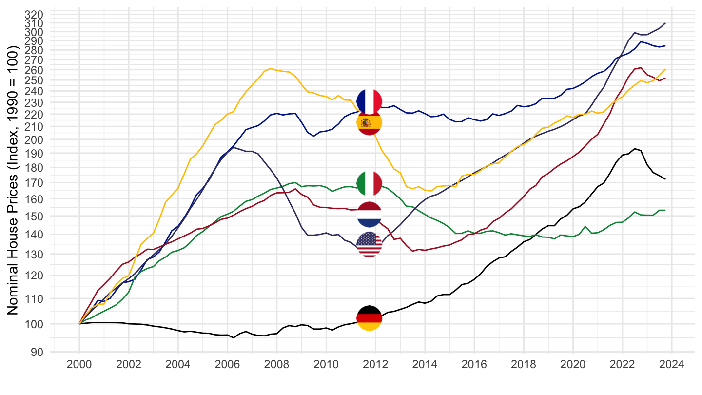
Japan, United States, United Kingdom
Code
SELECTED_PP %>%
  filter(iso3c %in% c("JPN", "GBR", "USA"),
         FREQ == "Q",
         date >= as.Date("1970-01-01"),
         VALUE == "N",
         UNIT_MEASURE == 628) %>%
  left_join(colors, by = c("Reference area" = "country")) %>%
  ggplot(.) + theme_minimal() + xlab("") + ylab("Real House Prices (Index, 2010 = 100)") +
  geom_line(aes(x = date, y = value, color = color)) +
  scale_color_identity() + add_flags +
  scale_x_date(breaks = seq(1900, 2100, 5) %>% paste0("-01-01") %>% as.Date,
               labels = date_format("%Y")) +
  scale_y_log10(breaks = seq(0, 600, 10),
                     labels = dollar_format(a = 1, prefix = "")) +
  theme(legend.position = c(0.8, 0.2),
        legend.title = element_blank())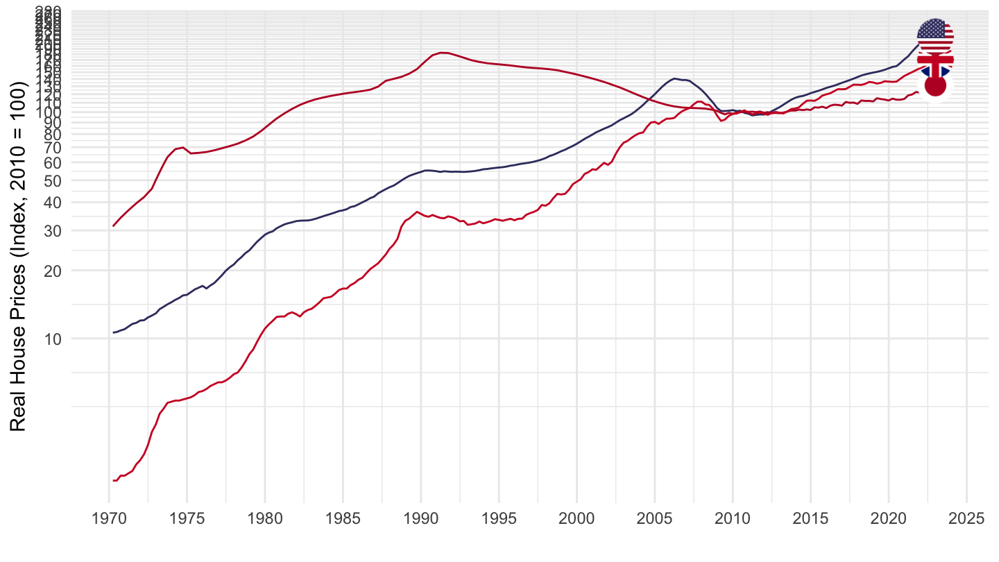
Germany, France, Sweden, Japan
1970-
Code
SELECTED_PP %>%
  filter(iso3c %in% c("DEU", "FRA", "JPN", "SWE"),
         FREQ == "Q",
         date >= as.Date("1970-01-01"),
         VALUE == "N",
         UNIT_MEASURE == 628) %>%
  left_join(colors, by = c("Reference area" = "country")) %>%
  ggplot(.) + theme_minimal() + xlab("") + ylab("Real House Prices (Index, 2010 = 100)") +
  geom_line(aes(x = date, y = value, color = color)) +
  scale_color_identity() + add_flags +
  scale_x_date(breaks = seq(1900, 2100, 5) %>% paste0("-01-01") %>% as.Date,
               labels = date_format("%Y")) +
  scale_y_log10(breaks = seq(0, 600, 10),
                     labels = dollar_format(a = 1, prefix = "")) +
  theme(legend.position = c(0.8, 0.2),
        legend.title = element_blank())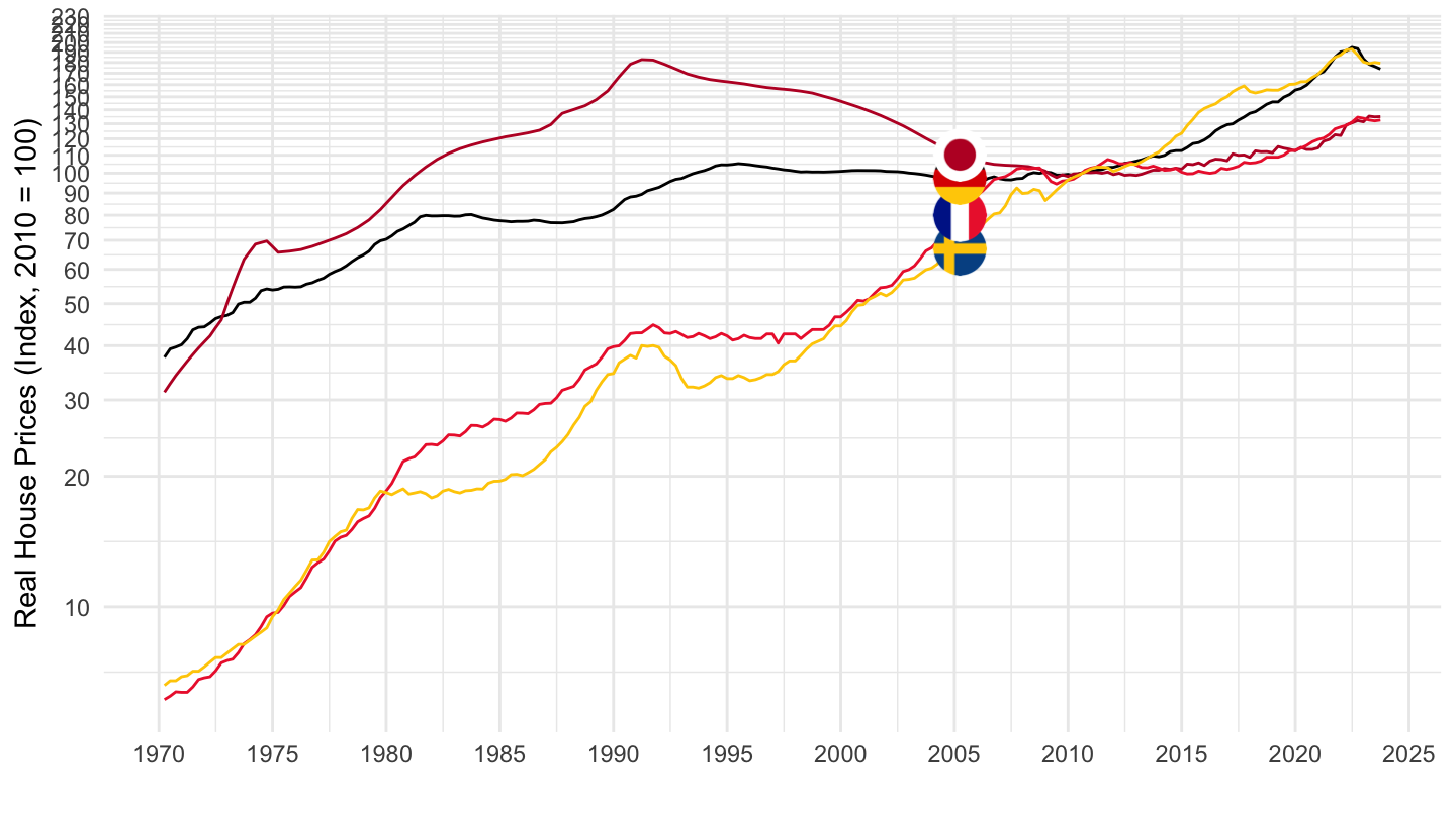
1998-
Code
SELECTED_PP %>%
  filter(iso3c %in% c("DEU", "FRA", "JPN", "SWE"),
         FREQ == "Q",
         date >= as.Date("1998-01-01"),
         VALUE == "N",
         UNIT_MEASURE == 628) %>%
  left_join(colors, by = c("Reference area" = "country")) %>%
  ggplot(.) + theme_minimal() + xlab("") + ylab("Nominal House Prices (Index, 2010 = 100)") +
  geom_line(aes(x = date, y = value, color = color)) +
  scale_color_identity() + add_flags +
  scale_x_date(breaks = seq(1900, 2100, 2) %>% paste0("-01-01") %>% as.Date,
               labels = date_format("%Y")) +
  scale_y_log10(breaks = seq(0, 600, 10),
                     labels = dollar_format(a = 1, prefix = "")) +
  theme(legend.position = c(0.8, 0.2),
        legend.title = element_blank())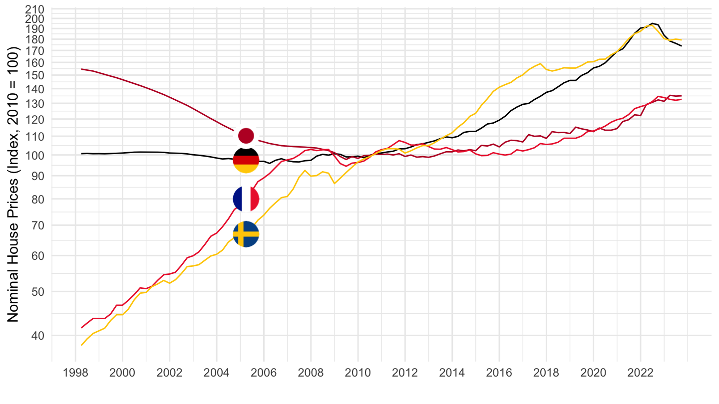
Germany, France, Italy
All
Code
SELECTED_PP %>%
  filter(iso3c %in% c("DEU", "FRA", "ITA"),
         FREQ == "Q",
         date >= as.Date("1970-01-01"),
         VALUE == "N",
         UNIT_MEASURE == 628) %>%
  left_join(colors, by = c("Reference area" = "country")) %>%
  ggplot(.) + theme_minimal() + xlab("") + ylab("Real House Prices (Index, 2010 = 100)") +
  geom_line(aes(x = date, y = value, color = color)) +
  scale_color_identity() + add_flags +
  scale_x_date(breaks = seq(1900, 2100, 5) %>% paste0("-01-01") %>% as.Date,
               labels = date_format("%Y")) +
  scale_y_log10(breaks = seq(0, 600, 10),
                     labels = dollar_format(a = 1, prefix = "")) +
  theme(legend.position = c(0.8, 0.2),
        legend.title = element_blank())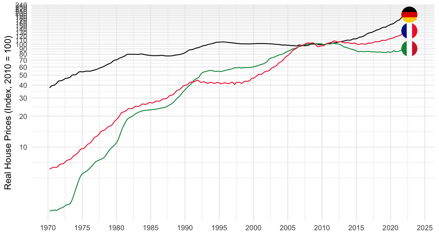
1990-
Code
SELECTED_PP %>%
  filter(iso3c %in% c("DEU", "FRA", "ITA"),
         FREQ == "Q",
         date >= as.Date("1989-12-31"),
         VALUE == "N",
         UNIT_MEASURE == 628) %>%
  left_join(colors, by = c("Reference area" = "country")) %>%
  group_by(iso3c) %>%
  mutate(value = 100*value/value[date == as.Date("1989-12-31")]) %>%
  ggplot(.) + theme_minimal() + xlab("") + ylab("Nominal House Prices (Index, 1990 = 100)") +
  geom_line(aes(x = date, y = value, color = color)) +
  scale_color_identity() + add_flags +
  scale_x_date(breaks = seq(1900, 2100, 5) %>% paste0("-01-01") %>% as.Date,
               labels = date_format("%Y")) +
  scale_y_log10(breaks = seq(0, 600, 10),
                     labels = dollar_format(a = 1, prefix = "")) +
  theme(legend.position = c(0.8, 0.2),
        legend.title = element_blank())
2000-
Code
SELECTED_PP %>%
  filter(iso3c %in% c("DEU", "FRA", "ITA"),
         FREQ == "Q",
         date >= as.Date("1999-12-31"),
         VALUE == "N",
         UNIT_MEASURE == 628) %>%
  left_join(colors, by = c("Reference area" = "country")) %>%
  group_by(iso3c) %>%
  mutate(value = 100*value/value[date == as.Date("1999-12-31")]) %>%
  ggplot(.) + theme_minimal() + xlab("") + ylab("Nominal House Prices (Index, 2000 = 100)") +
  geom_line(aes(x = date, y = value, color = color)) +
  scale_color_identity() + add_flags +
  scale_x_date(breaks = seq(1900, 2100, 2) %>% paste0("-01-01") %>% as.Date,
               labels = date_format("%Y")) +
  scale_y_log10(breaks = seq(0, 600, 10),
                     labels = dollar_format(a = 1, prefix = "")) +
  theme(legend.position = c(0.8, 0.2),
        legend.title = element_blank())
2008-
Code
SELECTED_PP %>%
  filter(iso3c %in% c("DEU", "FRA", "ITA"),
         FREQ == "Q",
         date >= as.Date("2007-12-31"),
         VALUE == "N",
         UNIT_MEASURE == 628) %>%
  left_join(colors, by = c("Reference area" = "country")) %>%
  group_by(iso3c) %>%
  mutate(value = 100*value/value[date == as.Date("2007-12-31")]) %>%
  ggplot(.) + theme_minimal() + xlab("") + ylab("Real House Prices (Index, 1998 = 100)") +
  geom_line(aes(x = date, y = value, color = color)) +
  scale_color_identity() + add_flags +
  scale_x_date(breaks = seq(1900, 2100, 2) %>% paste0("-01-01") %>% as.Date,
               labels = date_format("%Y")) +
  scale_y_log10(breaks = seq(0, 600, 10),
                     labels = dollar_format(a = 1, prefix = "")) +
  theme(legend.position = c(0.8, 0.2),
        legend.title = element_blank())
2021Q4-
Code
SELECTED_PP %>%
  filter(iso3c %in% c("DEU", "FRA", "ITA", "ESP", "NLD"),
         FREQ == "Q",
         zoo::as.yearqtr(OBS_TIME, format = "%Y-Q%q") >= zoo::as.yearqtr("2021 Q4"),
         VALUE == "N",
         UNIT_MEASURE == 628) %>%
  mutate(date = zoo::as.yearqtr(OBS_TIME, format = "%Y-Q%q")) %>%
  left_join(colors, by = c("Reference area" = "country")) %>%
  mutate(color = ifelse(iso3c == "FRA", color2, color)) %>%
  group_by(iso3c) %>%
  mutate(value = 100*value/value[date == zoo::as.yearqtr("2021 Q4")]) %>%
  ggplot(.) + theme_minimal() + xlab("") + ylab("Nominal House Prices (Index, 2020 = 100)") +
  geom_line(aes(x = date, y = value, color = color)) +
  scale_color_identity() + add_flags +
  scale_y_log10(breaks = seq(0, 600, 2),
                     labels = dollar_format(a = 1, prefix = "")) +
  zoo::scale_x_yearqtr(format = "%YQ%q") +
  theme(legend.position = c(0.8, 0.2),
        legend.title = element_blank(),
        axis.text.x = element_text(angle = 45, vjust = 1, hjust = 1))
Denmark, Germany, Switzerland
Code
SELECTED_PP %>%
  filter(iso3c %in% c("DEU", "DNK", "CHE"),
         FREQ == "Q",
         date >= as.Date("1970-01-01"),
         VALUE == "N",
         UNIT_MEASURE == 628) %>%
  left_join(colors, by = c("Reference area" = "country")) %>%
  ggplot(.) + theme_minimal() + xlab("") + ylab("Real House Prices (Index, 2010 = 100)") +
  geom_line(aes(x = date, y = value, color = color)) +
  scale_color_identity() + add_flags +
  scale_x_date(breaks = seq(1900, 2100, 5) %>% paste0("-01-01") %>% as.Date,
               labels = date_format("%Y")) +
  scale_y_log10(breaks = seq(0, 600, 10),
                     labels = dollar_format(a = 1, prefix = "")) +
  theme(legend.position = c(0.8, 0.2),
        legend.title = element_blank())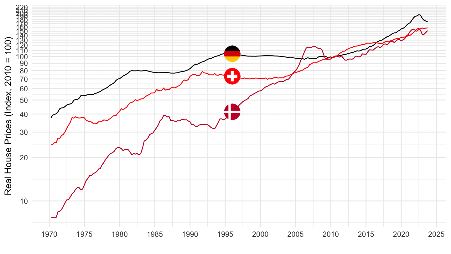
Individual Countries
Italy
Code
SELECTED_PP %>%
  filter(iso3c %in% c("ITA"),
         FREQ == "Q",
         UNIT_MEASURE == 628) %>%
  ggplot(.) + theme_minimal() + xlab("") + ylab("House Prices (Index, 2010 = 100)") +
  geom_line(aes(x = date, y = value, color = Value, linetype = Value)) +
  scale_x_date(breaks = seq(1900, 2100, 5) %>% paste0("-01-01") %>% as.Date,
               labels = date_format("%Y")) +
  scale_y_log10(breaks = seq(0, 600, 10),
                     labels = dollar_format(a = 1, prefix = "")) +
  scale_color_manual(values = viridis(3)[1:2]) +
  theme(legend.position = c(0.8, 0.2),
        legend.title = element_blank())
Japan
Code
SELECTED_PP %>%
  filter(iso3c %in% c("JPN"),
         FREQ == "Q",
         UNIT_MEASURE == 628) %>%
  ggplot(.) + theme_minimal() + xlab("") + ylab("House Prices (Index, 2010 = 100)") +
  geom_line(aes(x = date, y = value, color = Value, linetype = Value)) +
  scale_x_date(breaks = seq(1900, 2100, 5) %>% paste0("-01-01") %>% as.Date,
               labels = date_format("%Y")) +
  scale_y_log10(breaks = seq(0, 600, 10),
                     labels = dollar_format(a = 1, prefix = "")) +
  scale_color_manual(values = viridis(3)[1:2]) +
  theme(legend.position = c(0.8, 0.2),
        legend.title = element_blank())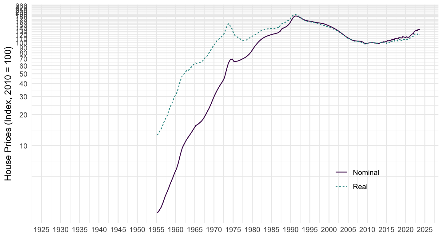
South Africa
Code
SELECTED_PP %>%
  filter(iso3c %in% c("ZAF"),
         FREQ == "Q",
         UNIT_MEASURE == 628) %>%
  ggplot(.) + theme_minimal() + xlab("") + ylab("House Prices (Index, 2010 = 100)") +
  geom_line(aes(x = date, y = value, color = Value, linetype = Value)) +
  scale_x_date(breaks = seq(1900, 2100, 5) %>% paste0("-01-01") %>% as.Date,
               labels = date_format("%Y")) +
  scale_y_log10(breaks = seq(0, 600, 10),
                     labels = dollar_format(a = 1, prefix = "")) +
  scale_color_manual(values = viridis(3)[1:2]) +
  theme(legend.position = c(0.8, 0.2),
        legend.title = element_blank())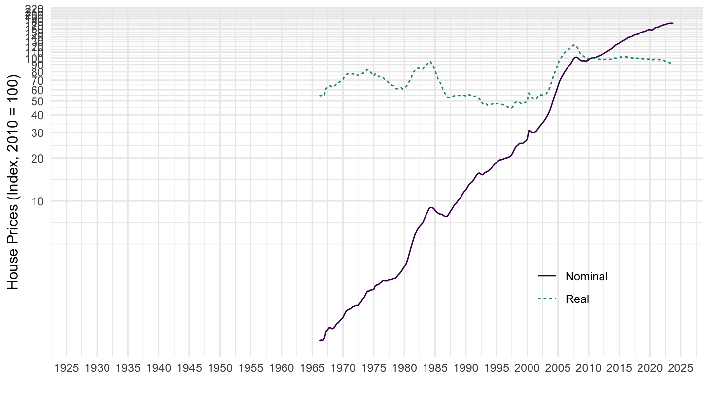
United Kingdom
Code
SELECTED_PP %>%
  filter(iso3c %in% c("GBR"),
         FREQ == "Q",
         UNIT_MEASURE == 628) %>%
  ggplot(.) + theme_minimal() + xlab("") + ylab("House Prices (Index, 2010 = 100)") +
  geom_line(aes(x = date, y = value, color = Value, linetype = Value)) +
  scale_x_date(breaks = seq(1900, 2100, 5) %>% paste0("-01-01") %>% as.Date,
               labels = date_format("%Y")) +
  scale_y_log10(breaks = seq(0, 600, 10),
                     labels = dollar_format(a = 1, prefix = "")) +
  scale_color_manual(values = viridis(3)[1:2]) +
  theme(legend.position = c(0.8, 0.2),
        legend.title = element_blank())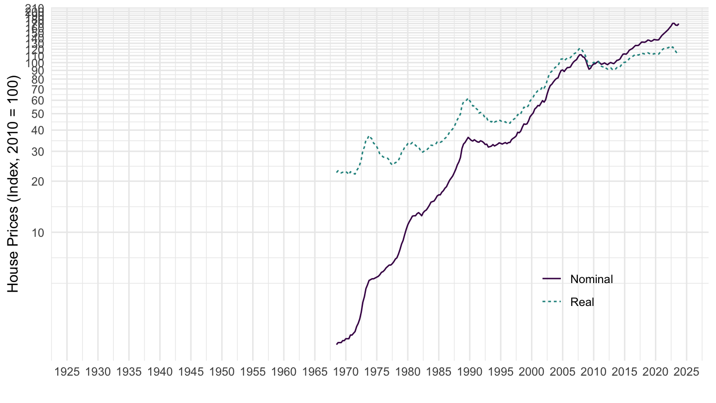
Australia
All
Code
SELECTED_PP %>%
  filter(iso3c %in% c("AUS"),
         FREQ == "Q",
         UNIT_MEASURE == 628) %>%
  ggplot(.) + theme_minimal() + xlab("") + ylab("House Prices (Index, 2010 = 100)") +
  geom_line(aes(x = date, y = value, color = Value, linetype = Value)) +
  scale_x_date(breaks = seq(1900, 2100, 5) %>% paste0("-01-01") %>% as.Date,
               labels = date_format("%Y")) +
  scale_y_log10(breaks = seq(0, 600, 10),
                     labels = dollar_format(a = 1, prefix = "")) +
  scale_color_manual(values = viridis(3)[1:2]) +
  theme(legend.position = c(0.8, 0.2),
        legend.title = element_blank())
2000-
Code
SELECTED_PP %>%
  filter(iso3c %in% c("AUS"),
         FREQ == "Q",
         UNIT_MEASURE == 628,
         date >= as.Date("2000-01-01")) %>%
  ggplot(.) + theme_minimal() + xlab("") + ylab("House Prices (Index, 2010 = 100)") +
  geom_line(aes(x = date, y = value, color = Value, linetype = Value)) +
  scale_x_date(breaks = seq(1900, 2100, 2) %>% paste0("-01-01") %>% as.Date,
               labels = date_format("%Y")) +
  scale_y_log10(breaks = seq(0, 600, 10),
                     labels = dollar_format(a = 1, prefix = "")) +
  scale_color_manual(values = viridis(3)[1:2]) +
  theme(legend.position = c(0.8, 0.2),
        legend.title = element_blank())
2010-
Code
SELECTED_PP %>%
  filter(iso3c %in% c("AUS"),
         FREQ == "Q",
         UNIT_MEASURE == 628,
         date >= as.Date("2010-01-01")) %>%
  ggplot(.) + theme_minimal() + xlab("") + ylab("House Prices (Index, 2010 = 100)") +
  geom_line(aes(x = date, y = value, color = Value, linetype = Value)) +
  scale_x_date(breaks = seq(1900, 2100, 1) %>% paste0("-01-01") %>% as.Date,
               labels = date_format("%Y")) +
  scale_y_log10(breaks = seq(0, 600, 10),
                     labels = dollar_format(a = 1, prefix = "")) +
  scale_color_manual(values = viridis(3)[1:2]) +
  theme(legend.position = c(0.8, 0.2),
        legend.title = element_blank())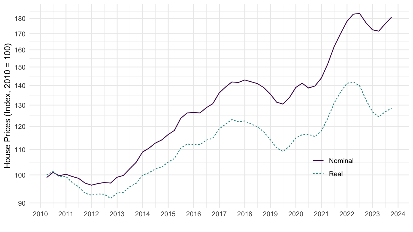
Belgium
Code
SELECTED_PP %>%
  filter(iso3c %in% c("BEL"),
         FREQ == "Q",
         UNIT_MEASURE == 628) %>%
  ggplot(.) + theme_minimal() + xlab("") + ylab("House Prices (Index, 2010 = 100)") +
  geom_line(aes(x = date, y = value, color = Value, linetype = Value)) +
  scale_x_date(breaks = seq(1900, 2100, 5) %>% paste0("-01-01") %>% as.Date,
               labels = date_format("%Y")) +
  scale_y_log10(breaks = seq(0, 600, 10),
                     labels = dollar_format(a = 1, prefix = "")) +
  scale_color_manual(values = viridis(3)[1:2]) +
  theme(legend.position = c(0.8, 0.2),
        legend.title = element_blank())
Canada
Code
SELECTED_PP %>%
  filter(iso3c %in% c("CAN"),
         FREQ == "Q",
         UNIT_MEASURE == 628) %>%
  ggplot(.) + theme_minimal() + xlab("") + ylab("House Prices (Index, 2010 = 100)") +
  geom_line(aes(x = date, y = value, color = Value, linetype = Value)) +
  scale_x_date(breaks = seq(1900, 2100, 5) %>% paste0("-01-01") %>% as.Date,
               labels = date_format("%Y")) +
  scale_y_log10(breaks = seq(0, 600, 10),
                     labels = dollar_format(a = 1, prefix = "")) +
  scale_color_manual(values = viridis(3)[1:2]) +
  theme(legend.position = c(0.8, 0.2),
        legend.title = element_blank())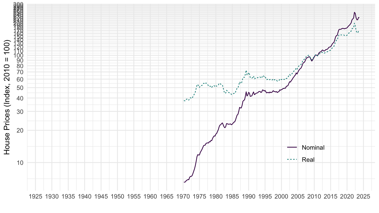
Switzerland
Code
SELECTED_PP %>%
  filter(iso3c %in% c("CHE"),
         FREQ == "Q",
         UNIT_MEASURE == 628) %>%
  ggplot(.) + theme_minimal() + xlab("") + ylab("House Prices (Index, 2010 = 100)") +
  geom_line(aes(x = date, y = value, color = Value, linetype = Value)) +
  scale_x_date(breaks = seq(1900, 2100, 5) %>% paste0("-01-01") %>% as.Date,
               labels = date_format("%Y")) +
  scale_y_log10(breaks = seq(0, 600, 10),
                     labels = dollar_format(a = 1, prefix = "")) +
  scale_color_manual(values = viridis(3)[1:2]) +
  theme(legend.position = c(0.8, 0.2),
        legend.title = element_blank())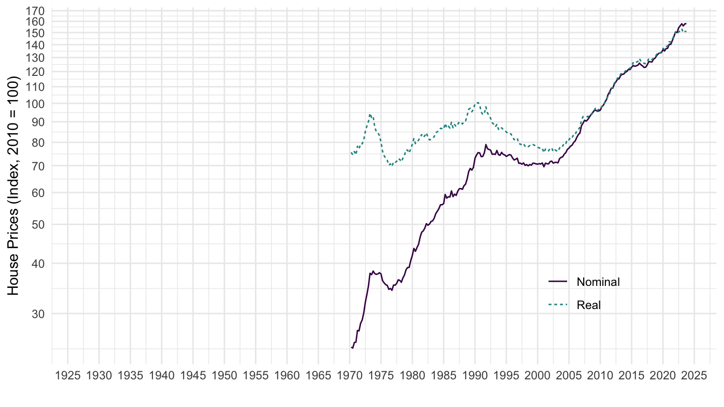
Germany
Code
SELECTED_PP %>%
  filter(iso3c %in% c("DEU"),
         FREQ == "Q",
         UNIT_MEASURE == 628) %>%
  ggplot(.) + theme_minimal() + xlab("") + ylab("House Prices (Index, 2010 = 100)") +
  geom_line(aes(x = date, y = value, color = Value, linetype = Value)) +
  scale_x_date(breaks = seq(1900, 2100, 5) %>% paste0("-01-01") %>% as.Date,
               labels = date_format("%Y")) +
  scale_y_log10(breaks = seq(0, 600, 10),
                     labels = dollar_format(a = 1, prefix = "")) +
  scale_color_manual(values = viridis(3)[1:2]) +
  theme(legend.position = c(0.8, 0.2),
        legend.title = element_blank())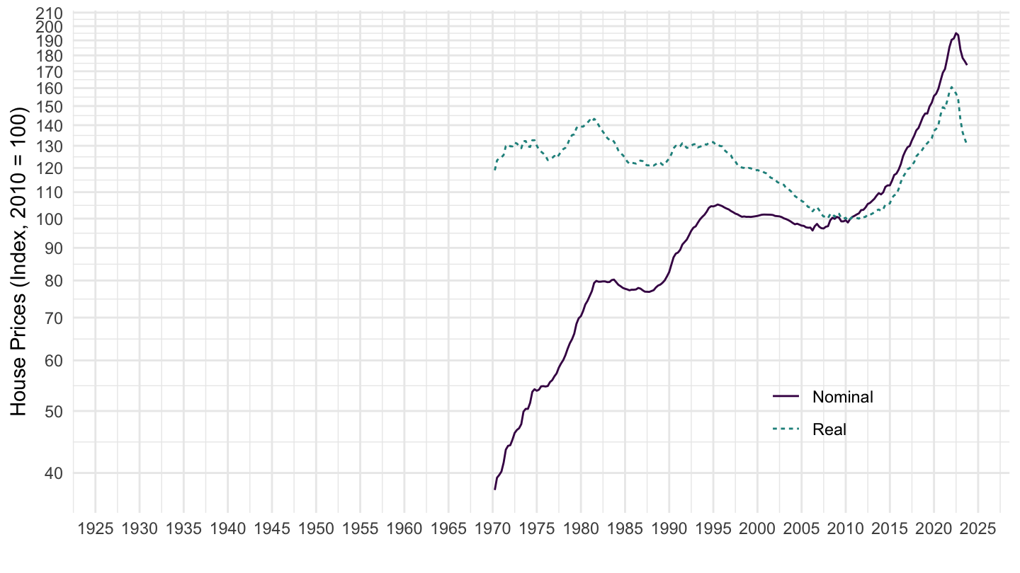
Denmark
Code
SELECTED_PP %>%
  filter(iso3c %in% c("DNK"),
         FREQ == "Q",
         UNIT_MEASURE == 628) %>%
  ggplot(.) + theme_minimal() + xlab("") + ylab("House Prices (Index, 2010 = 100)") +
  geom_line(aes(x = date, y = value, color = Value, linetype = Value)) +
  scale_x_date(breaks = seq(1900, 2100, 5) %>% paste0("-01-01") %>% as.Date,
               labels = date_format("%Y")) +
  scale_y_log10(breaks = seq(0, 600, 10),
                     labels = dollar_format(a = 1, prefix = "")) +
  scale_color_manual(values = viridis(3)[1:2]) +
  theme(legend.position = c(0.8, 0.2),
        legend.title = element_blank())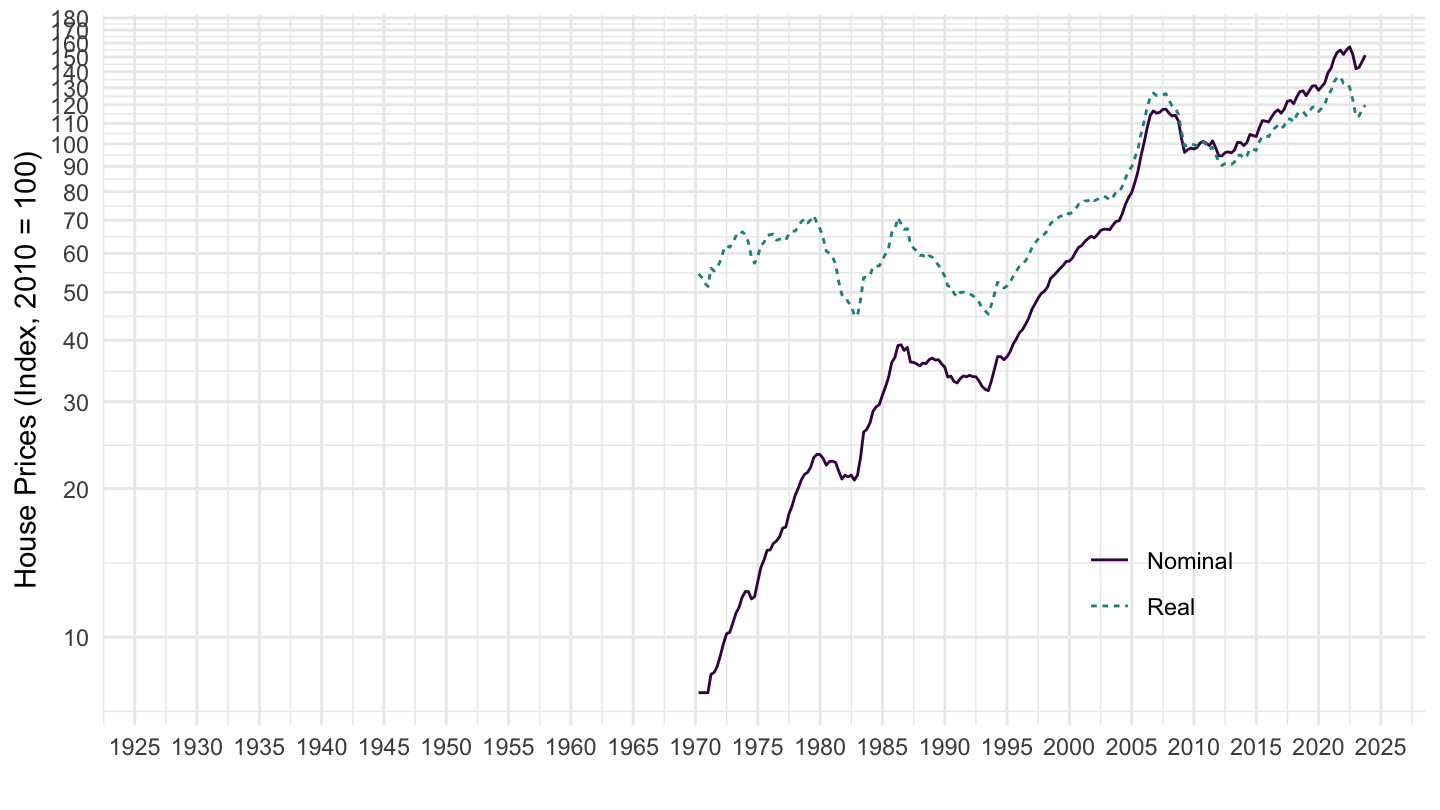
Finland
Code
SELECTED_PP %>%
  filter(iso3c %in% c("FIN"),
         FREQ == "Q",
         UNIT_MEASURE == 628) %>%
  ggplot(.) + theme_minimal() + xlab("") + ylab("House Prices (Index, 2010 = 100)") +
  geom_line(aes(x = date, y = value, color = Value, linetype = Value)) +
  scale_x_date(breaks = seq(1900, 2100, 5) %>% paste0("-01-01") %>% as.Date,
               labels = date_format("%Y")) +
  scale_y_log10(breaks = seq(0, 600, 10),
                     labels = dollar_format(a = 1, prefix = "")) +
  scale_color_manual(values = viridis(3)[1:2]) +
  theme(legend.position = c(0.8, 0.2),
        legend.title = element_blank())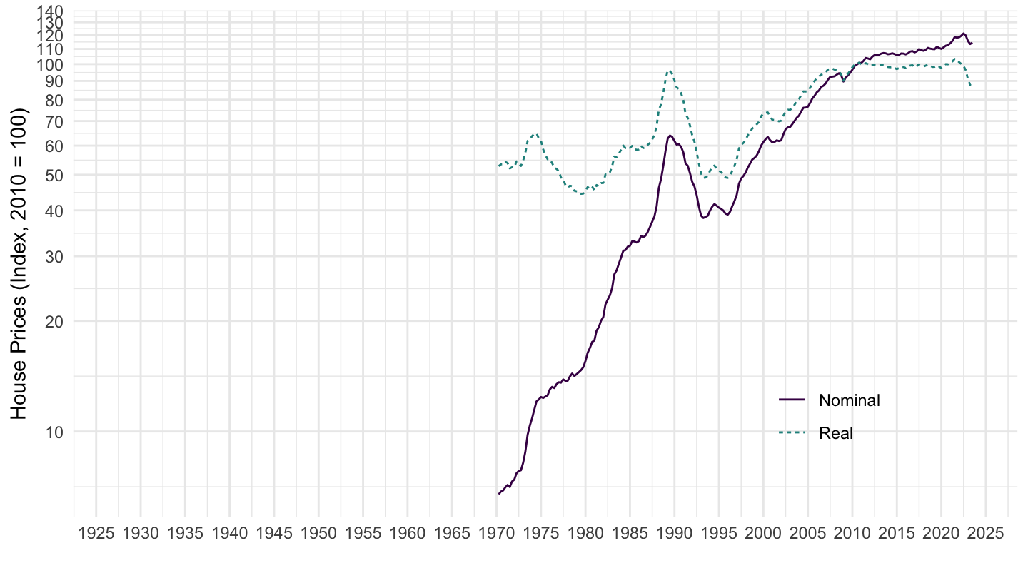
France
Code
SELECTED_PP %>%
  filter(iso3c %in% c("FRA"),
         FREQ == "Q",
         date >= as.Date("1970-01-01"),
         UNIT_MEASURE == 628) %>%
  ggplot(.) + theme_minimal() + xlab("") + ylab("House Prices (Index, 2010 = 100)") +
  geom_line(aes(x = date, y = value, color = Value, linetype = Value)) +
  scale_x_date(breaks = seq(1900, 2100, 5) %>% paste0("-01-01") %>% as.Date,
               labels = date_format("%Y")) +
  scale_y_log10(breaks = c(seq(1, 10, 1), seq(0, 600, 10)),
                     labels = dollar_format(a = 1, prefix = "")) +
  scale_color_manual(values = viridis(3)[1:2]) +
  theme(legend.position = c(0.8, 0.2),
        legend.title = element_blank())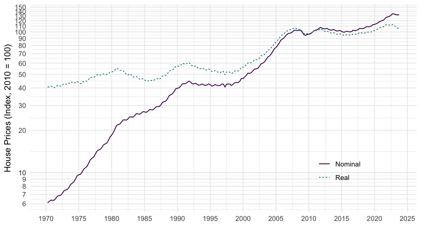
Ireland
Code
SELECTED_PP %>%
  filter(iso3c %in% c("IRL"),
         FREQ == "Q",
         UNIT_MEASURE == 628) %>%
  ggplot(.) + theme_minimal() + xlab("") + ylab("House Prices (Index, 2010 = 100)") +
  geom_line(aes(x = date, y = value, color = Value, linetype = Value)) +
  scale_x_date(breaks = seq(1900, 2100, 5) %>% paste0("-01-01") %>% as.Date,
               labels = date_format("%Y")) +
  scale_y_log10(breaks = seq(0, 600, 10),
                     labels = dollar_format(a = 1, prefix = "")) +
  scale_color_manual(values = viridis(3)[1:2]) +
  theme(legend.position = c(0.8, 0.2),
        legend.title = element_blank())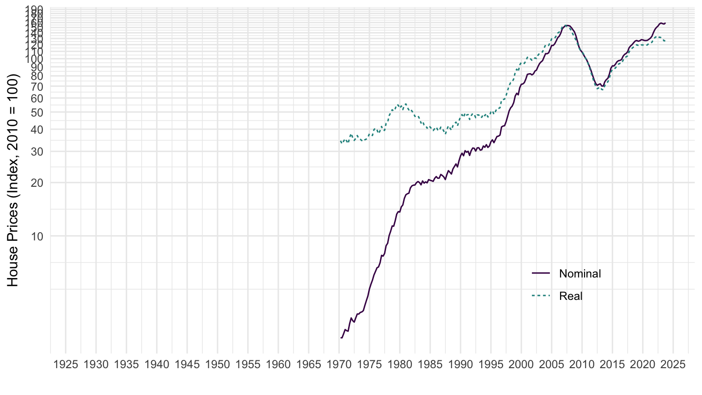
Netherlands
Code
SELECTED_PP %>%
  filter(iso3c %in% c("NLD"),
         FREQ == "Q",
         UNIT_MEASURE == 628) %>%
  ggplot(.) + theme_minimal() + xlab("") + ylab("House Prices (Index, 2010 = 100)") +
  geom_line(aes(x = date, y = value, color = Value, linetype = Value)) +
  scale_x_date(breaks = seq(1900, 2100, 5) %>% paste0("-01-01") %>% as.Date,
               labels = date_format("%Y")) +
  scale_y_log10(breaks = seq(0, 600, 10),
                     labels = dollar_format(a = 1, prefix = "")) +
  scale_color_manual(values = viridis(3)[1:2]) +
  theme(legend.position = c(0.8, 0.2),
        legend.title = element_blank())
New Zealand
Code
SELECTED_PP %>%
  filter(iso3c %in% c("NZL"),
         FREQ == "Q",
         UNIT_MEASURE == 628) %>%
  ggplot(.) + theme_minimal() + xlab("") + ylab("House Prices (Index, 2010 = 100)") +
  geom_line(aes(x = date, y = value, color = Value, linetype = Value)) +
  scale_x_date(breaks = seq(1900, 2100, 5) %>% paste0("-01-01") %>% as.Date,
               labels = date_format("%Y")) +
  scale_y_log10(breaks = seq(0, 600, 10),
                     labels = dollar_format(a = 1, prefix = "")) +
  scale_color_manual(values = viridis(3)[1:2]) +
  theme(legend.position = c(0.8, 0.2),
        legend.title = element_blank())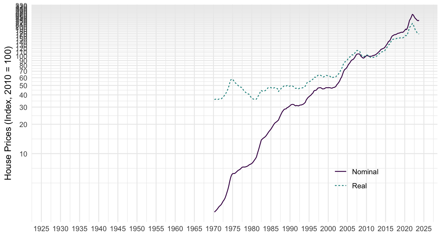
Sweden
Code
SELECTED_PP %>%
  filter(iso3c %in% c("SWE"),
         FREQ == "Q",
         UNIT_MEASURE == 628) %>%
  ggplot(.) + theme_minimal() + xlab("") + ylab("House Prices (Index, 2010 = 100)") +
  geom_line(aes(x = date, y = value, color = Value, linetype = Value)) +
  scale_x_date(breaks = seq(1900, 2100, 5) %>% paste0("-01-01") %>% as.Date,
               labels = date_format("%Y")) +
  scale_y_log10(breaks = seq(0, 600, 10),
                     labels = dollar_format(a = 1, prefix = "")) +
  scale_color_manual(values = viridis(3)[1:2]) +
  theme(legend.position = c(0.8, 0.2),
        legend.title = element_blank())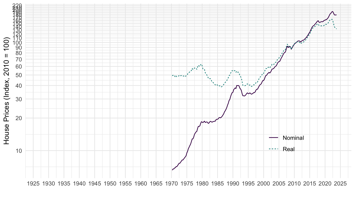
Sweden (1980 - 2000)
Code
SELECTED_PP %>%
  filter(iso3c %in% c("SWE"),
         FREQ == "Q",
         UNIT_MEASURE == 628,
         date >= as.Date("1980-01-01"),
         date <= as.Date("2000-01-01")) %>%
  ggplot(.) + theme_minimal() + xlab("") + ylab("House Prices (Index, 2010 = 100)") +
  geom_line(aes(x = date, y = value, color = Value, linetype = Value)) +
  scale_x_date(breaks = seq(1900, 2100, 2) %>% paste0("-01-01") %>% as.Date,
               labels = date_format("%Y")) +
  scale_y_log10(breaks = seq(0, 600, 5),
                     labels = dollar_format(a = 1, prefix = "")) +
  scale_color_manual(values = viridis(3)[1:2]) +
  theme(legend.position = c(0.8, 0.2),
        legend.title = element_blank())
United States
Code
SELECTED_PP %>%
  filter(iso3c %in% c("USA"),
         FREQ == "Q",
         UNIT_MEASURE == 628) %>%
  ggplot(.) + theme_minimal() + xlab("") + ylab("House Prices (Index, 2010 = 100)") +
  geom_line(aes(x = date, y = value, color = Value, linetype = Value)) +
  scale_x_date(breaks = seq(1900, 2100, 5) %>% paste0("-01-01") %>% as.Date,
               labels = date_format("%Y")) +
  scale_y_log10(breaks = seq(0, 600, 10),
                     labels = dollar_format(a = 1, prefix = "")) +
  scale_color_manual(values = viridis(3)[1:2]) +
  theme(legend.position = c(0.8, 0.2),
        legend.title = element_blank())
Spain
Code
SELECTED_PP %>%
  filter(iso3c %in% c("ESP"),
         FREQ == "Q",
         date >= as.Date("1970-01-01"),
         UNIT_MEASURE == 628) %>%
  ggplot(.) + theme_minimal() + xlab("") + ylab("House Prices (Index, 2010 = 100)") +
  geom_line(aes(x = date, y = value, color = Value, linetype = Value)) +
  scale_x_date(breaks = seq(1900, 2100, 5) %>% paste0("-01-01") %>% as.Date,
               labels = date_format("%Y")) +
  scale_y_log10(breaks = c(seq(1, 10, 1), seq(0, 600, 10)),
                     labels = dollar_format(a = 1, prefix = "")) +
  scale_color_manual(values = viridis(3)[1:2]) +
  theme(legend.position = c(0.8, 0.2),
        legend.title = element_blank())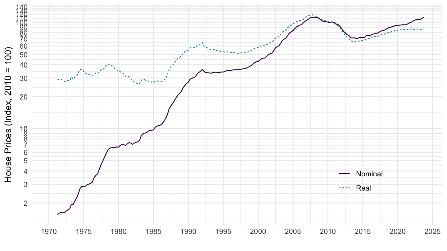
Korea
Code
SELECTED_PP %>%
  filter(iso3c %in% c("KOR"),
         FREQ == "Q",
         date >= as.Date("1970-01-01"),
         UNIT_MEASURE == 628) %>%
  ggplot(.) + theme_minimal() + xlab("") + ylab("House Prices (Index, 2010 = 100)") +
  geom_line(aes(x = date, y = value, color = Value, linetype = Value)) +
  scale_x_date(breaks = seq(1900, 2100, 5) %>% paste0("-01-01") %>% as.Date,
               labels = date_format("%Y")) +
  scale_y_log10(breaks = c(seq(1, 10, 1), seq(0, 600, 10)),
                     labels = dollar_format(a = 1, prefix = "")) +
  scale_color_manual(values = viridis(3)[1:2]) +
  theme(legend.position = c(0.8, 0.2),
        legend.title = element_blank())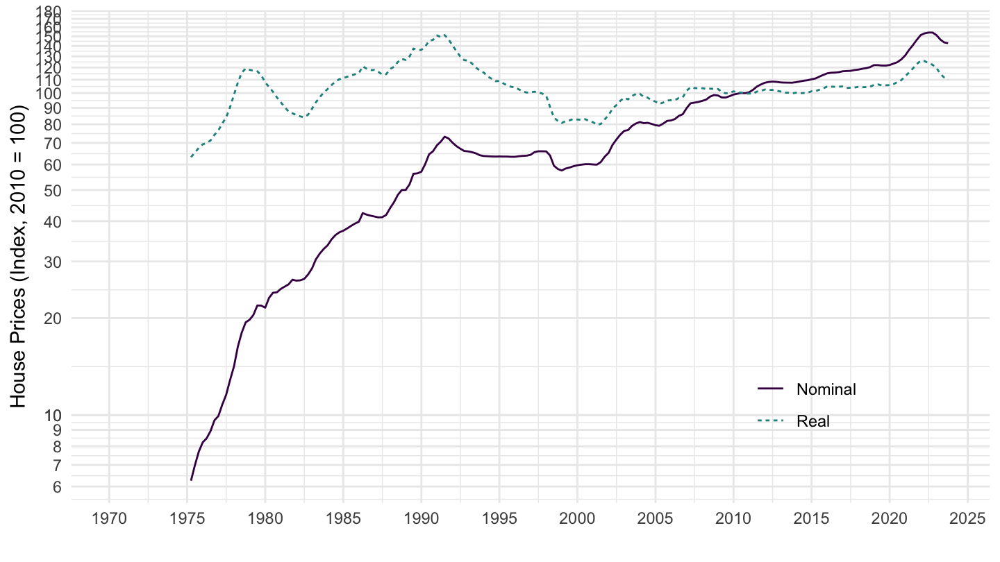
Euro Area
Code
SELECTED_PP %>%
  filter(`Reference area` %in% c("Euro area"),
         FREQ == "Q",
         UNIT_MEASURE == 628) %>%
  ggplot(.) + theme_minimal() + xlab("") + ylab("House Prices (Index, 2010 = 100)") +
  geom_line(aes(x = date, y = value, color = Value, linetype = Value)) +
  scale_x_date(breaks = seq(1900, 2100, 5) %>% paste0("-01-01") %>% as.Date,
               labels = date_format("%Y")) +
  scale_y_log10(breaks = seq(0, 600, 10),
                     labels = dollar_format(a = 1, prefix = "")) +
  scale_color_manual(values = viridis(3)[1:2]) +
  theme(legend.position = c(0.8, 0.2),
        legend.title = element_blank())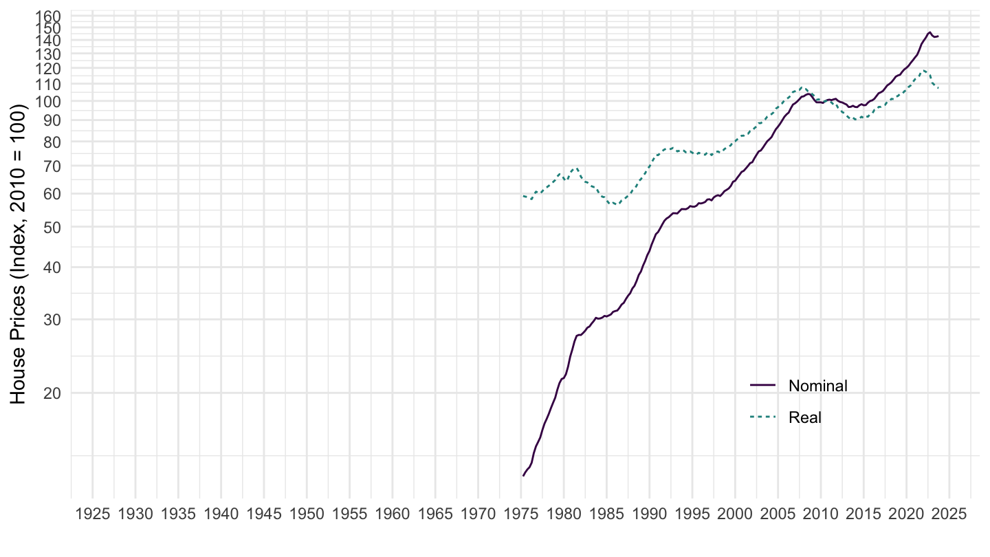
Hong Kong
Code
SELECTED_PP %>%
  filter(iso3c %in% c("HKG"),
         FREQ == "Q",
         UNIT_MEASURE == 628) %>%
  ggplot(.) + theme_minimal() + xlab("") + ylab("House Prices (Index, 2010 = 100)") +
  geom_line(aes(x = date, y = value, color = Value, linetype = Value)) +
  scale_x_date(breaks = seq(1900, 2100, 5) %>% paste0("-01-01") %>% as.Date,
               labels = date_format("%Y")) +
  scale_y_log10(breaks = seq(0, 600, 10),
                     labels = dollar_format(a = 1, prefix = "")) +
  scale_color_manual(values = viridis(3)[1:2]) +
  theme(legend.position = c(0.8, 0.2),
        legend.title = element_blank())
Norway
Code
SELECTED_PP %>%
  filter(iso3c %in% c("NOR"),
         FREQ == "Q",
         UNIT_MEASURE == 628) %>%
  ggplot(.) + theme_minimal() + xlab("") + ylab("House Prices (Index, 2010 = 100)") +
  geom_line(aes(x = date, y = value, color = Value, linetype = Value)) +
  scale_x_date(breaks = seq(1900, 2100, 5) %>% paste0("-01-01") %>% as.Date,
               labels = date_format("%Y")) +
  scale_y_log10(breaks = seq(0, 600, 10),
                     labels = dollar_format(a = 1, prefix = "")) +
  scale_color_manual(values = viridis(3)[1:2]) +
  theme(legend.position = c(0.8, 0.2),
        legend.title = element_blank())
Colombia
Code
SELECTED_PP %>%
  filter(iso3c %in% c("COL"),
         FREQ == "Q",
         UNIT_MEASURE == 628) %>%
  ggplot(.) + theme_minimal() + xlab("") + ylab("House Prices (Index, 2010 = 100)") +
  geom_line(aes(x = date, y = value, color = Value, linetype = Value)) +
  scale_x_date(breaks = seq(1900, 2100, 5) %>% paste0("-01-01") %>% as.Date,
               labels = date_format("%Y")) +
  scale_y_log10(breaks = seq(0, 600, 10),
                     labels = dollar_format(a = 1, prefix = "")) +
  scale_color_manual(values = viridis(3)[1:2]) +
  theme(legend.position = c(0.8, 0.2),
        legend.title = element_blank())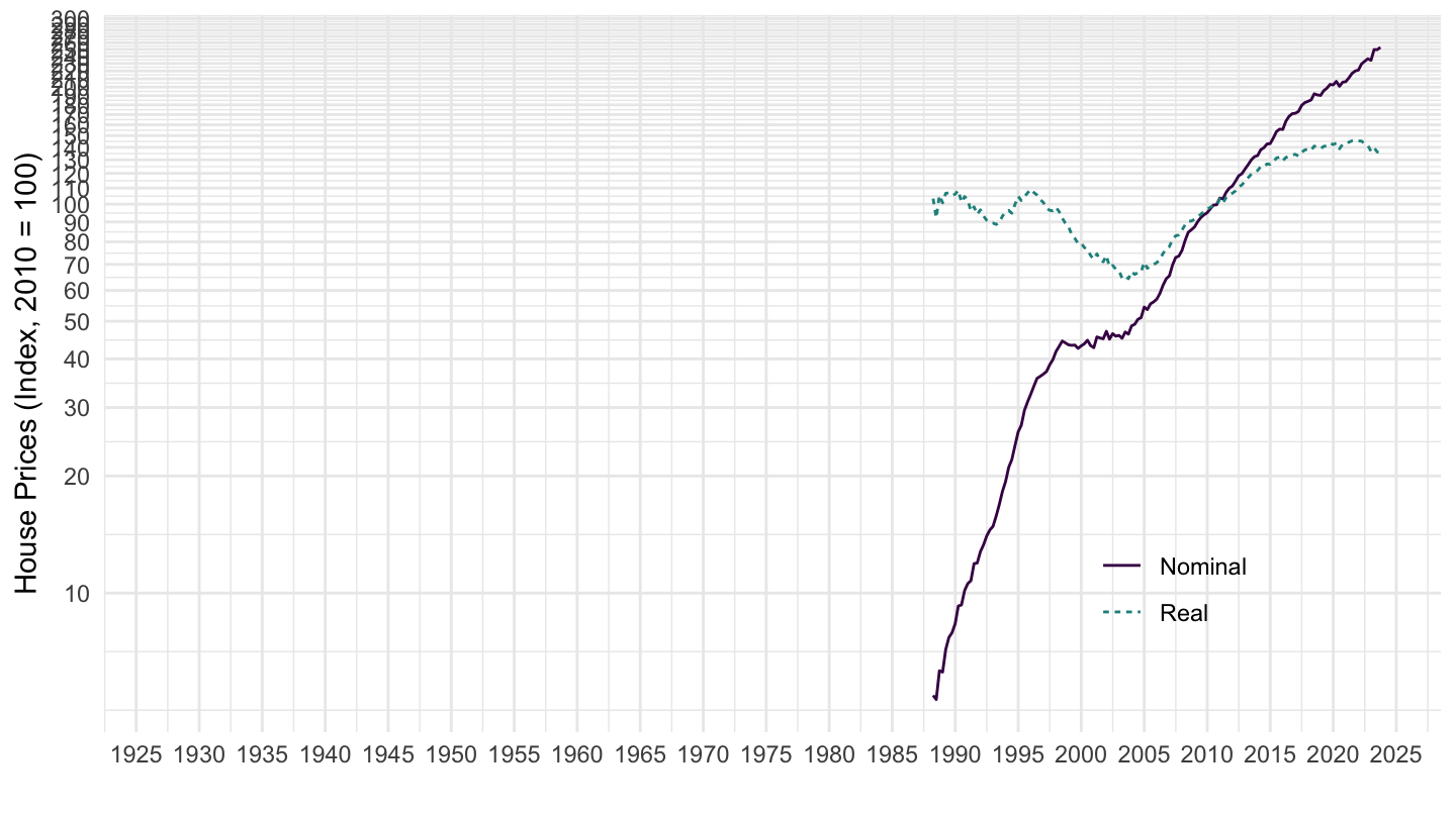
Malaysia
Code
SELECTED_PP %>%
  filter(iso3c %in% c("MYS"),
         FREQ == "Q",
         UNIT_MEASURE == 628) %>%
  ggplot(.) + theme_minimal() + xlab("") + ylab("House Prices (Index, 2010 = 100)") +
  geom_line(aes(x = date, y = value, color = Value, linetype = Value)) +
  scale_x_date(breaks = seq(1900, 2100, 5) %>% paste0("-01-01") %>% as.Date,
               labels = date_format("%Y")) +
  scale_y_log10(breaks = seq(0, 600, 10),
                     labels = dollar_format(a = 1, prefix = "")) +
  scale_color_manual(values = viridis(3)[1:2]) +
  theme(legend.position = c(0.8, 0.2),
        legend.title = element_blank())
Thailand
Code
SELECTED_PP %>%
  filter(iso3c %in% c("THA"),
         FREQ == "Q",
         UNIT_MEASURE == 628) %>%
  ggplot(.) + theme_minimal() + xlab("") + ylab("House Prices (Index, 2010 = 100)") +
  geom_line(aes(x = date, y = value, color = Value, linetype = Value)) +
  scale_x_date(breaks = seq(1900, 2100, 5) %>% paste0("-01-01") %>% as.Date,
               labels = date_format("%Y")) +
  scale_y_log10(breaks = seq(0, 600, 10),
                     labels = dollar_format(a = 1, prefix = "")) +
  scale_color_manual(values = viridis(3)[1:2]) +
  theme(legend.position = c(0.8, 0.2),
        legend.title = element_blank())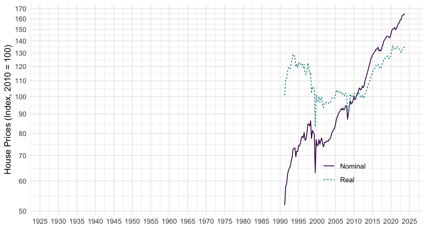
Israel
Code
SELECTED_PP %>%
  filter(iso3c %in% c("ISR"),
         FREQ == "Q",
         UNIT_MEASURE == 628) %>%
  ggplot(.) + theme_minimal() + xlab("") + ylab("House Prices (Index, 2010 = 100)") +
  geom_line(aes(x = date, y = value, color = Value, linetype = Value)) +
  scale_x_date(breaks = seq(1900, 2100, 5) %>% paste0("-01-01") %>% as.Date,
               labels = date_format("%Y")) +
  scale_y_log10(breaks = seq(0, 600, 10),
                     labels = dollar_format(a = 1, prefix = "")) +
  scale_color_manual(values = viridis(3)[1:2]) +
  theme(legend.position = c(0.8, 0.2),
        legend.title = element_blank())
Peru
Code
SELECTED_PP %>%
  filter(iso3c %in% c("PER"),
         FREQ == "Q",
         UNIT_MEASURE == 628) %>%
  ggplot(.) + theme_minimal() + xlab("") + ylab("House Prices (Index, 2010 = 100)") +
  geom_line(aes(x = date, y = value, color = Value, linetype = Value)) +
  scale_x_date(breaks = seq(1900, 2100, 5) %>% paste0("-01-01") %>% as.Date,
               labels = date_format("%Y")) +
  scale_y_log10(breaks = seq(0, 600, 10),
                     labels = dollar_format(a = 1, prefix = "")) +
  scale_color_manual(values = viridis(3)[1:2]) +
  theme(legend.position = c(0.8, 0.2),
        legend.title = element_blank())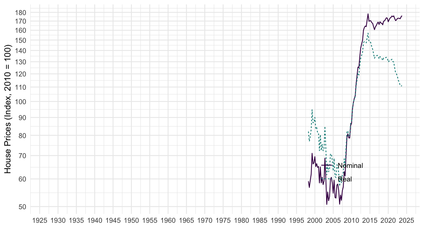
Singapore
Code
SELECTED_PP %>%
  filter(iso3c %in% c("SGP"),
         FREQ == "Q",
         UNIT_MEASURE == 628) %>%
  ggplot(.) + theme_minimal() + xlab("") + ylab("House Prices (Index, 2010 = 100)") +
  geom_line(aes(x = date, y = value, color = Value, linetype = Value)) +
  scale_x_date(breaks = seq(1900, 2100, 5) %>% paste0("-01-01") %>% as.Date,
               labels = date_format("%Y")) +
  scale_y_log10(breaks = seq(0, 600, 10),
                     labels = dollar_format(a = 1, prefix = "")) +
  scale_color_manual(values = viridis(3)[1:2]) +
  theme(legend.position = c(0.8, 0.2),
        legend.title = element_blank())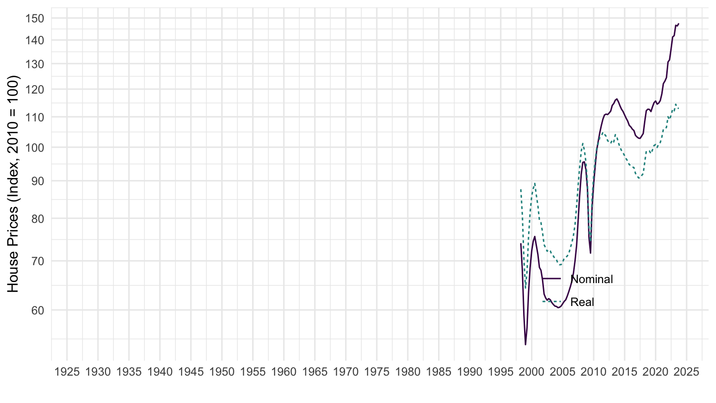
Lithuania
Code
SELECTED_PP %>%
  filter(iso3c %in% c("LTU"),
         FREQ == "Q",
         UNIT_MEASURE == 628) %>%
  ggplot(.) + theme_minimal() + xlab("") + ylab("House Prices (Index, 2010 = 100)") +
  geom_line(aes(x = date, y = value, color = Value, linetype = Value)) +
  scale_x_date(breaks = seq(1900, 2100, 5) %>% paste0("-01-01") %>% as.Date,
               labels = date_format("%Y")) +
  scale_y_log10(breaks = seq(0, 600, 10),
                     labels = dollar_format(a = 1, prefix = "")) +
  scale_color_manual(values = viridis(3)[1:2]) +
  theme(legend.position = c(0.8, 0.2),
        legend.title = element_blank())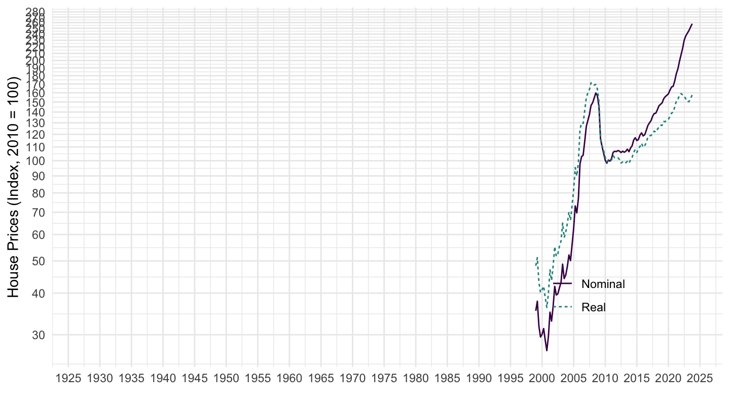
Austria
Code
SELECTED_PP %>%
  filter(iso3c %in% c("AUT"),
         FREQ == "Q",
         UNIT_MEASURE == 628) %>%
  ggplot(.) + theme_minimal() + xlab("") + ylab("House Prices (Index, 2010 = 100)") +
  geom_line(aes(x = date, y = value, color = Value, linetype = Value)) +
  scale_x_date(breaks = seq(1900, 2100, 5) %>% paste0("-01-01") %>% as.Date,
               labels = date_format("%Y")) +
  scale_y_log10(breaks = seq(0, 600, 10),
                     labels = dollar_format(a = 1, prefix = "")) +
  scale_color_manual(values = viridis(3)[1:2]) +
  theme(legend.position = c(0.8, 0.2),
        legend.title = element_blank())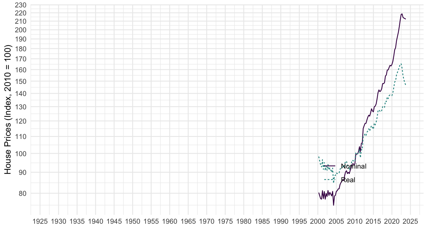
Iceland
Code
SELECTED_PP %>%
  filter(iso3c %in% c("ISL"),
         FREQ == "Q",
         UNIT_MEASURE == 628) %>%
  ggplot(.) + theme_minimal() + xlab("") + ylab("House Prices (Index, 2010 = 100)") +
  geom_line(aes(x = date, y = value, color = Value)) +
  scale_x_date(breaks = seq(1900, 2100, 2) %>% paste0("-01-01") %>% as.Date,
               labels = date_format("%Y")) +
  scale_y_log10(breaks = seq(0, 600, 10),
                     labels = dollar_format(a = 1, prefix = "")) +
  scale_color_manual(values = viridis(3)[1:2]) +
  theme(legend.position = c(0.8, 0.2),
        legend.title = element_blank())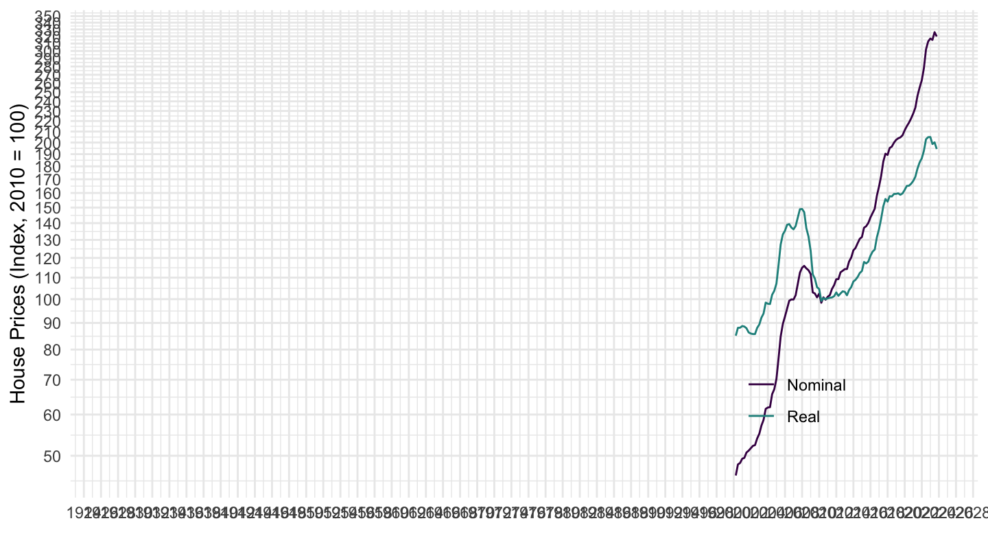
North Macedonia
Code
SELECTED_PP %>%
  filter(iso3c %in% c("MKD"),
         FREQ == "Q",
         UNIT_MEASURE == 628) %>%
  ggplot(.) + theme_minimal() + xlab("") + ylab("House Prices (Index, 2010 = 100)") +
  geom_line(aes(x = date, y = value, color = Value, linetype = Value)) +
  scale_x_date(breaks = seq(1900, 2100, 5) %>% paste0("-01-01") %>% as.Date,
               labels = date_format("%Y")) +
  scale_y_log10(breaks = seq(0, 600, 10),
                     labels = dollar_format(a = 1, prefix = "")) +
  scale_color_manual(values = viridis(3)[1:2]) +
  theme(legend.position = c(0.8, 0.2),
        legend.title = element_blank())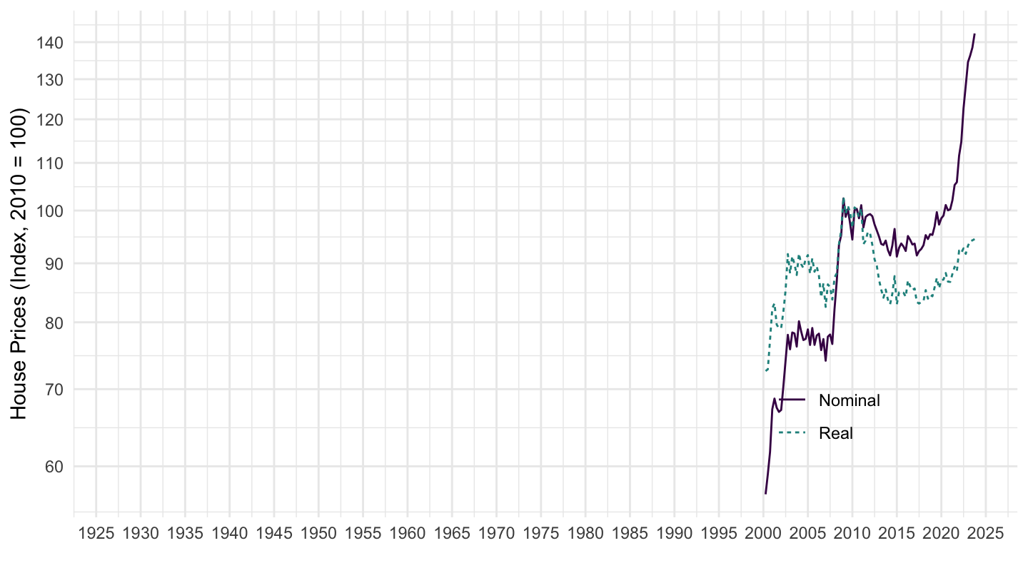
Serbia
Code
SELECTED_PP %>%
  filter(iso3c %in% c("SRB"),
         FREQ == "Q",
         UNIT_MEASURE == 628) %>%
  ggplot(.) + theme_minimal() + xlab("") + ylab("House Prices (Index, 2010 = 100)") +
  geom_line(aes(x = date, y = value, color = Value, linetype = Value)) +
  scale_x_date(breaks = seq(1900, 2100, 2) %>% paste0("-01-01") %>% as.Date,
               labels = date_format("%Y")) +
  scale_y_log10(breaks = seq(0, 600, 10),
                     labels = dollar_format(a = 1, prefix = "")) +
  scale_color_manual(values = viridis(3)[1:2]) +
  theme(legend.position = c(0.8, 0.2),
        legend.title = element_blank())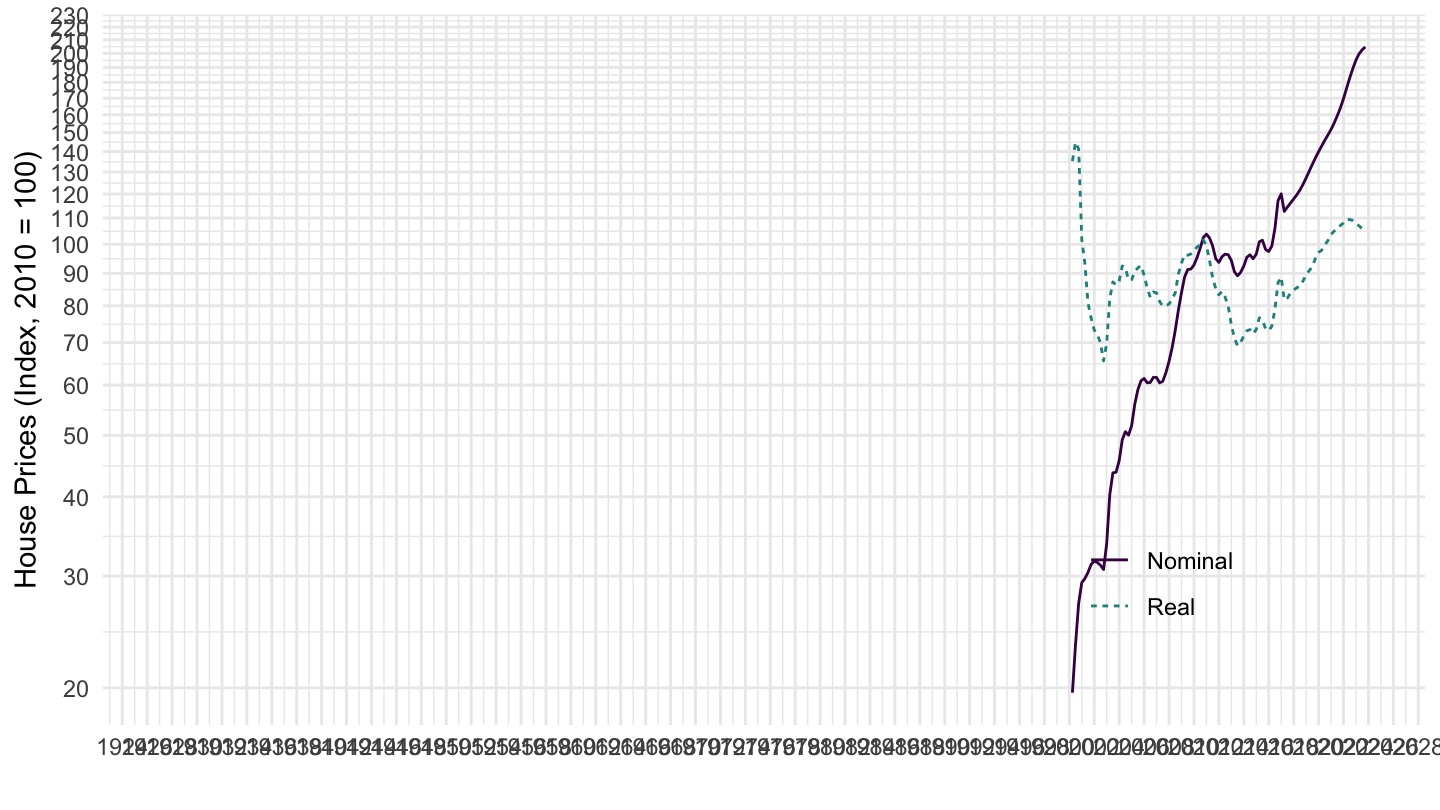
Brazil
Code
SELECTED_PP %>%
  filter(iso3c %in% c("BRA"),
         FREQ == "Q",
         UNIT_MEASURE == 628) %>%
  ggplot(.) + theme_minimal() + xlab("") + ylab("House Prices (Index, 2010 = 100)") +
  geom_line(aes(x = date, y = value, color = Value, linetype = Value)) +
  scale_x_date(breaks = seq(1900, 2100, 2) %>% paste0("-01-01") %>% as.Date,
               labels = date_format("%Y")) +
  scale_y_log10(breaks = seq(0, 600, 10),
                     labels = dollar_format(a = 1, prefix = "")) +
  scale_color_manual(values = viridis(3)[1:2]) +
  theme(legend.position = c(0.8, 0.2),
        legend.title = element_blank())
Russia
Code
SELECTED_PP %>%
  filter(iso3c %in% c("RUS"),
         FREQ == "Q",
         UNIT_MEASURE == 628) %>%
  ggplot(.) + theme_minimal() + xlab("") + ylab("House Prices (Index, 2010 = 100)") +
  geom_line(aes(x = date, y = value, color = Value, linetype = Value)) +
  scale_x_date(breaks = seq(1900, 2100, 2) %>% paste0("-01-01") %>% as.Date,
               labels = date_format("%Y")) +
  scale_y_log10(breaks = seq(0, 600, 10),
                     labels = dollar_format(a = 1, prefix = "")) +
  scale_color_manual(values = viridis(3)[1:2]) +
  theme(legend.position = c(0.8, 0.2),
        legend.title = element_blank())
Croatia
Code
SELECTED_PP %>%
  filter(iso3c %in% c("HRV"),
         FREQ == "Q",
         UNIT_MEASURE == 628) %>%
  ggplot(.) + theme_minimal() + xlab("") + ylab("House Prices (Index, 2010 = 100)") +
  geom_line(aes(x = date, y = value, color = Value, linetype = Value)) +
  scale_x_date(breaks = seq(1900, 2100, 2) %>% paste0("-01-01") %>% as.Date,
               labels = date_format("%Y")) +
  scale_y_log10(breaks = seq(0, 600, 10),
                     labels = dollar_format(a = 1, prefix = "")) +
  scale_color_manual(values = viridis(3)[1:2]) +
  theme(legend.position = c(0.8, 0.2),
        legend.title = element_blank())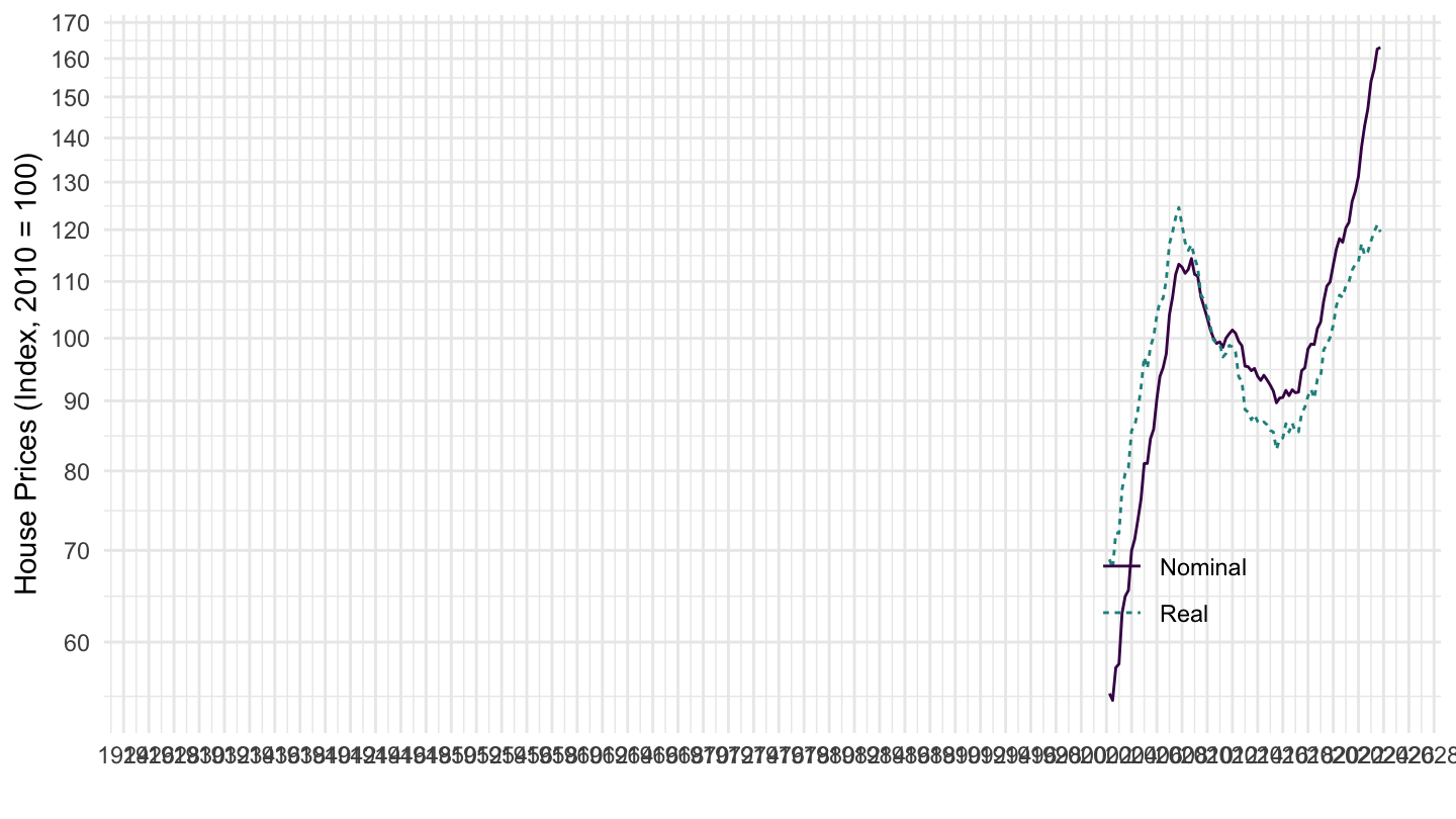
Indonesia
Code
SELECTED_PP %>%
  filter(iso3c %in% c("IDN"),
         FREQ == "Q",
         UNIT_MEASURE == 628) %>%
  ggplot(.) + theme_minimal() + xlab("") + ylab("House Prices (Index, 2010 = 100)") +
  geom_line(aes(x = date, y = value, color = Value, linetype = Value)) +
  scale_x_date(breaks = seq(1900, 2100, 2) %>% paste0("-01-01") %>% as.Date,
               labels = date_format("%Y")) +
  scale_y_log10(breaks = seq(0, 600, 10),
                     labels = dollar_format(a = 1, prefix = "")) +
  scale_color_manual(values = viridis(3)[1:2]) +
  theme(legend.position = c(0.8, 0.2),
        legend.title = element_blank())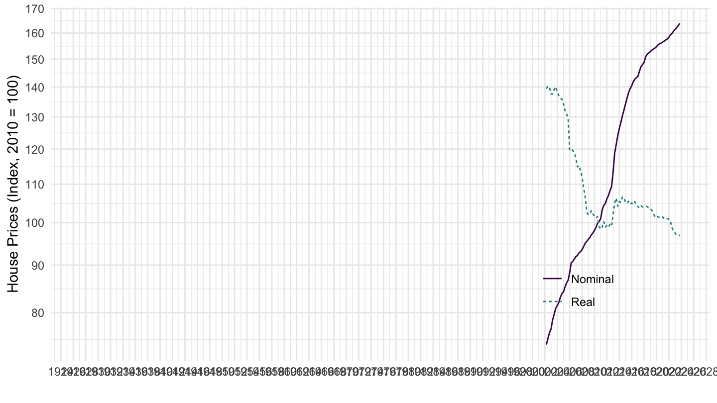
Chile
Code
SELECTED_PP %>%
  filter(iso3c %in% c("CHL"),
         FREQ == "Q",
         UNIT_MEASURE == 628) %>%
  ggplot(.) + theme_minimal() + xlab("") + ylab("House Prices (Index, 2010 = 100)") +
  geom_line(aes(x = date, y = value, color = Value, linetype = Value)) +
  scale_x_date(breaks = seq(1900, 2100, 2) %>% paste0("-01-01") %>% as.Date,
               labels = date_format("%Y")) +
  scale_y_log10(breaks = seq(0, 600, 10),
                     labels = dollar_format(a = 1, prefix = "")) +
  scale_color_manual(values = viridis(3)[1:2]) +
  theme(legend.position = c(0.8, 0.2),
        legend.title = element_blank())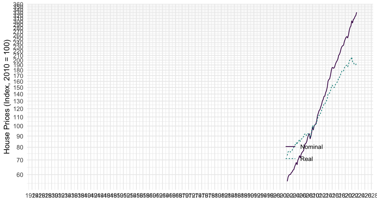
Cyprus
Code
SELECTED_PP %>%
  filter(iso3c %in% c("CYP"),
         FREQ == "Q",
         UNIT_MEASURE == 628) %>%
  ggplot(.) + theme_minimal() + xlab("") + ylab("House Prices (Index, 2010 = 100)") +
  geom_line(aes(x = date, y = value, color = Value, linetype = Value)) +
  scale_x_date(breaks = seq(1900, 2100, 2) %>% paste0("-01-01") %>% as.Date,
               labels = date_format("%Y")) +
  scale_y_log10(breaks = seq(0, 600, 10),
                     labels = dollar_format(a = 1, prefix = "")) +
  scale_color_manual(values = viridis(3)[1:2]) +
  theme(legend.position = c(0.8, 0.2),
        legend.title = element_blank())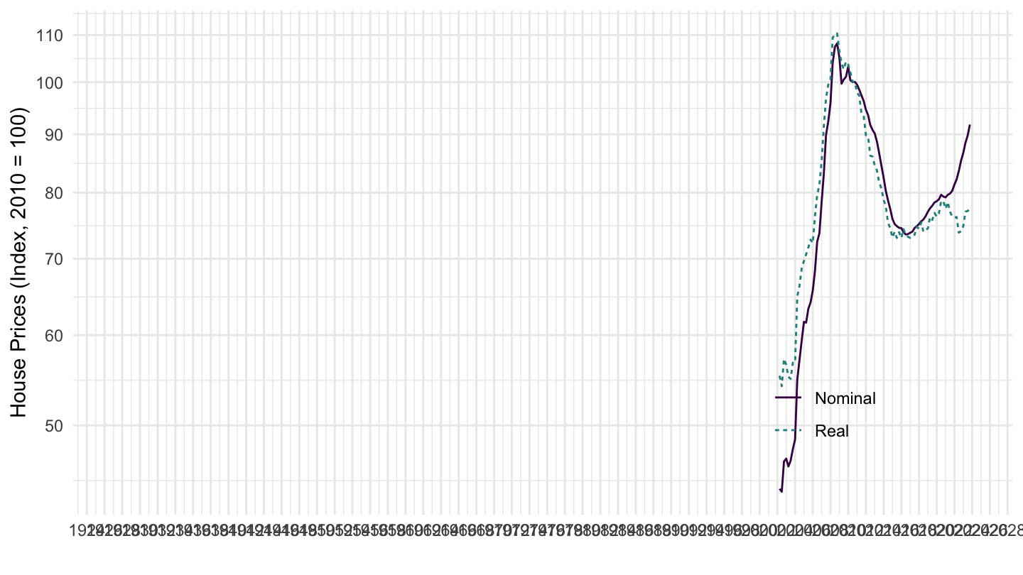
United Arab Emirates
Code
SELECTED_PP %>%
  filter(iso3c %in% c("ARE"),
         FREQ == "Q",
         UNIT_MEASURE == 628) %>%
  ggplot(.) + theme_minimal() + xlab("") + ylab("House Prices (Index, 2010 = 100)") +
  geom_line(aes(x = date, y = value, color = Value, linetype = Value)) +
  scale_x_date(breaks = seq(1900, 2100, 2) %>% paste0("-01-01") %>% as.Date,
               labels = date_format("%Y")) +
  scale_y_log10(breaks = seq(0, 600, 10),
                     labels = dollar_format(a = 1, prefix = "")) +
  scale_color_manual(values = viridis(3)[1:2]) +
  theme(legend.position = c(0.8, 0.2),
        legend.title = element_blank())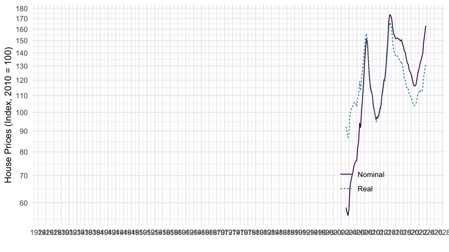
Bulgaria
Code
SELECTED_PP %>%
  filter(iso3c %in% c("BGR"),
         FREQ == "Q",
         UNIT_MEASURE == 628) %>%
  ggplot(.) + theme_minimal() + xlab("") + ylab("House Prices (Index, 2010 = 100)") +
  geom_line(aes(x = date, y = value, color = Value, linetype = Value)) +
  scale_x_date(breaks = seq(1900, 2100, 2) %>% paste0("-01-01") %>% as.Date,
               labels = date_format("%Y")) +
  scale_y_log10(breaks = seq(0, 600, 10),
                     labels = dollar_format(a = 1, prefix = "")) +
  scale_color_manual(values = viridis(3)[1:2]) +
  theme(legend.position = c(0.8, 0.2),
        legend.title = element_blank())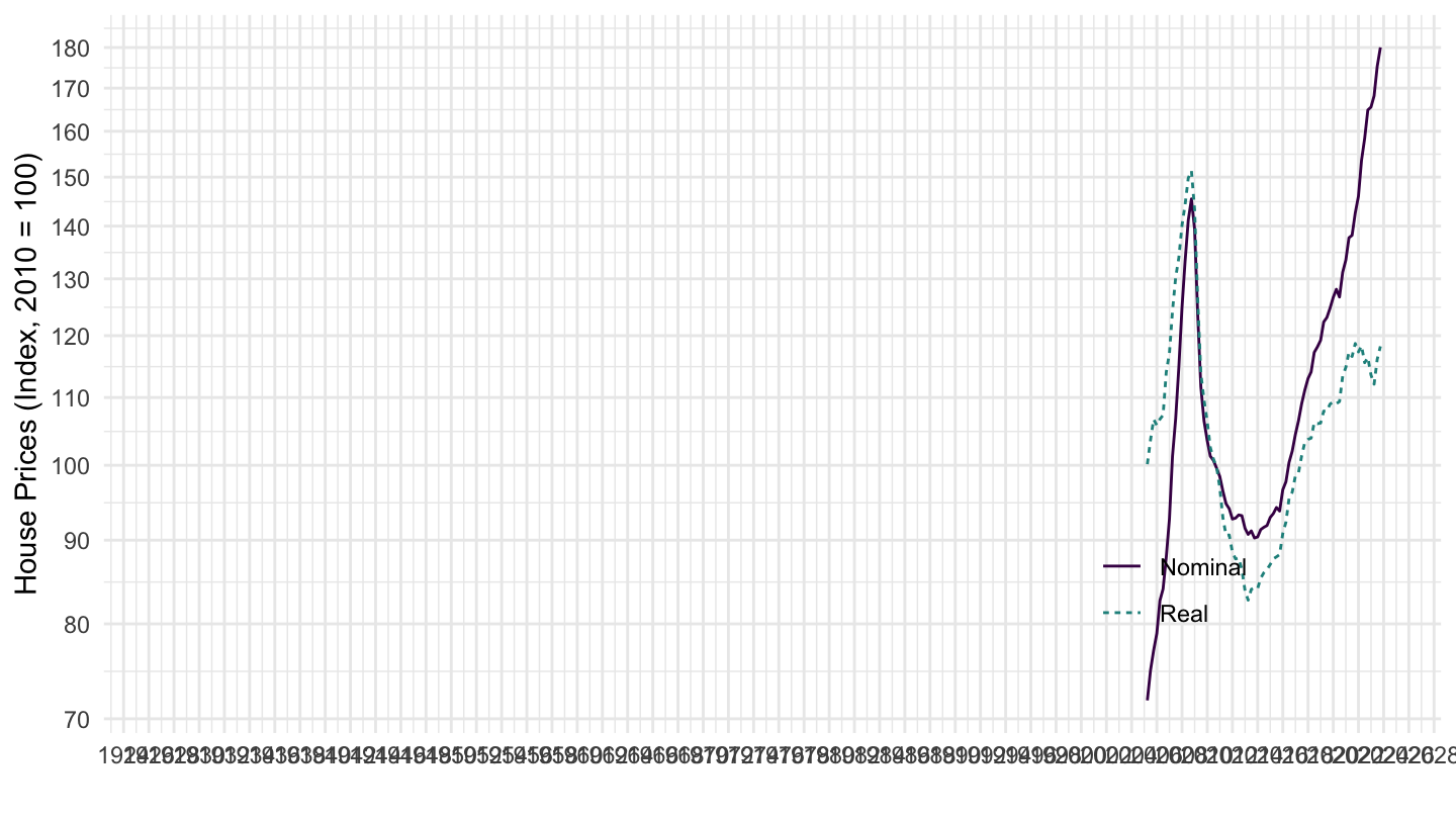
Estonia
Code
SELECTED_PP %>%
  filter(iso3c %in% c("EST"),
         FREQ == "Q",
         UNIT_MEASURE == 628) %>%
  ggplot(.) + theme_minimal() + xlab("") + ylab("House Prices (Index, 2010 = 100)") +
  geom_line(aes(x = date, y = value, color = Value, linetype = Value)) +
  scale_x_date(breaks = seq(1900, 2100, 2) %>% paste0("-01-01") %>% as.Date,
               labels = date_format("%Y")) +
  scale_y_log10(breaks = seq(0, 600, 10),
                     labels = dollar_format(a = 1, prefix = "")) +
  scale_color_manual(values = viridis(3)[1:2]) +
  theme(legend.position = c(0.8, 0.2),
        legend.title = element_blank())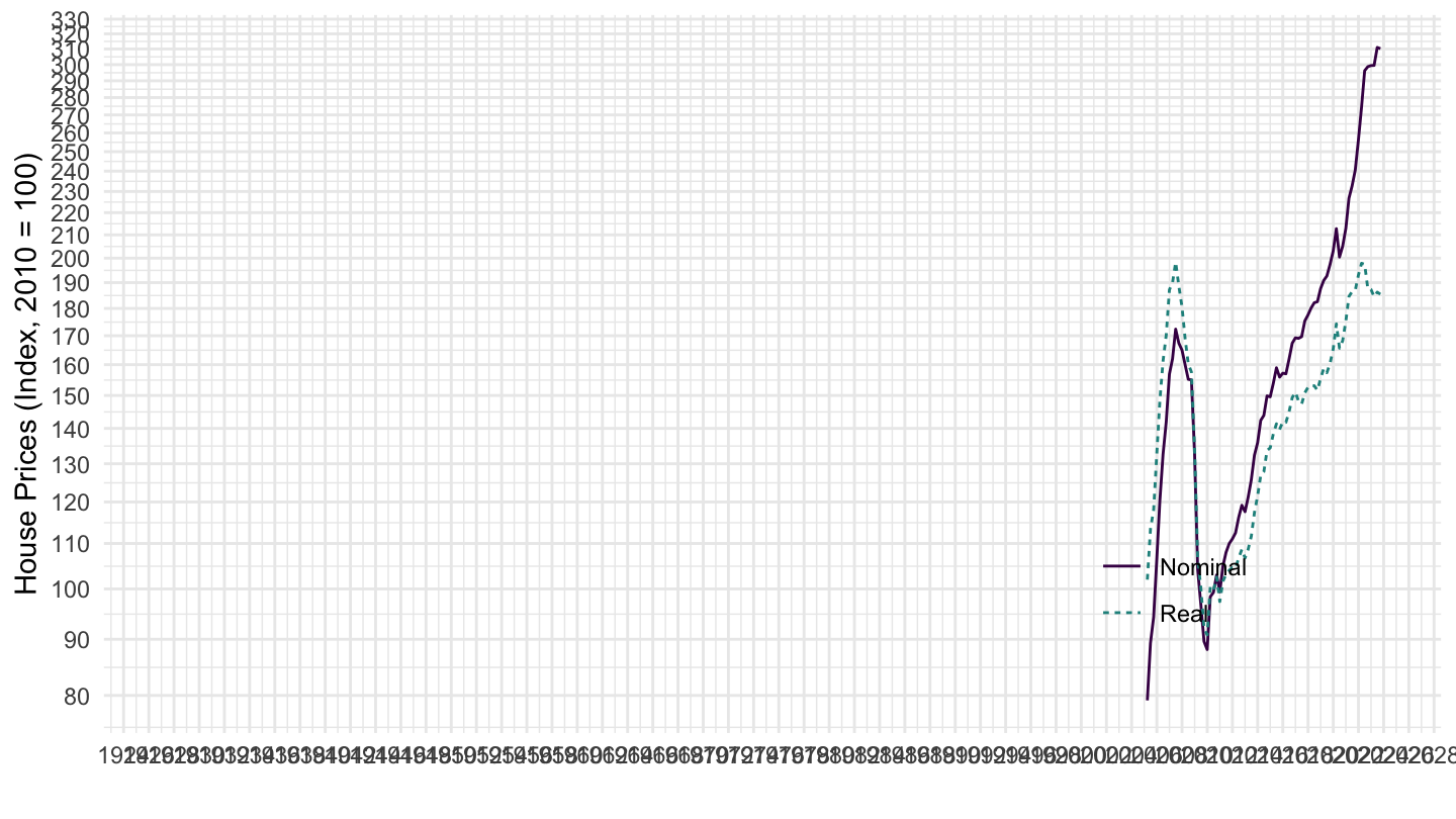
Mexico
Code
SELECTED_PP %>%
  filter(iso3c %in% c("MEX"),
         FREQ == "Q",
         UNIT_MEASURE == 628) %>%
  ggplot(.) + theme_minimal() + xlab("") + ylab("House Prices (Index, 2010 = 100)") +
  geom_line(aes(x = date, y = value, color = Value, linetype = Value)) +
  scale_x_date(breaks = seq(1900, 2100, 2) %>% paste0("-01-01") %>% as.Date,
               labels = date_format("%Y")) +
  scale_y_log10(breaks = seq(0, 600, 10),
                     labels = dollar_format(a = 1, prefix = "")) +
  scale_color_manual(values = viridis(3)[1:2]) +
  theme(legend.position = c(0.8, 0.2),
        legend.title = element_blank())
Malta
Code
SELECTED_PP %>%
  filter(iso3c %in% c("MLT"),
         FREQ == "Q",
         UNIT_MEASURE == 628) %>%
  ggplot(.) + theme_minimal() + xlab("") + ylab("House Prices (Index, 2010 = 100)") +
  geom_line(aes(x = date, y = value, color = Value, linetype = Value)) +
  scale_x_date(breaks = seq(1900, 2100, 2) %>% paste0("-01-01") %>% as.Date,
               labels = date_format("%Y")) +
  scale_y_log10(breaks = seq(0, 600, 10),
                     labels = dollar_format(a = 1, prefix = "")) +
  scale_color_manual(values = viridis(3)[1:2]) +
  theme(legend.position = c(0.8, 0.2),
        legend.title = element_blank())
China
Code
SELECTED_PP %>%
  filter(iso3c %in% c("CHN"),
         FREQ == "Q",
         UNIT_MEASURE == 628) %>%
  ggplot(.) + theme_minimal() + xlab("") + ylab("House Prices (Index, 2010 = 100)") +
  geom_line(aes(x = date, y = value, color = Value, linetype = Value)) +
  scale_x_date(breaks = seq(1900, 2100, 2) %>% paste0("-01-01") %>% as.Date,
               labels = date_format("%Y")) +
  scale_y_log10(breaks = seq(0, 600, 10),
                     labels = dollar_format(a = 1, prefix = "")) +
  scale_color_manual(values = viridis(3)[1:2]) +
  theme(legend.position = c(0.8, 0.2),
        legend.title = element_blank())
Greece
Code
SELECTED_PP %>%
  filter(iso3c %in% c("GRC"),
         FREQ == "Q",
         UNIT_MEASURE == 628) %>%
  ggplot(.) + theme_minimal() + xlab("") + ylab("House Prices (Index, 2010 = 100)") +
  geom_line(aes(x = date, y = value, color = Value, linetype = Value)) +
  scale_x_date(breaks = seq(1900, 2100, 2) %>% paste0("-01-01") %>% as.Date,
               labels = date_format("%Y")) +
  scale_y_log10(breaks = seq(0, 600, 10),
                     labels = dollar_format(a = 1, prefix = "")) +
  scale_color_manual(values = viridis(3)[1:2]) +
  theme(legend.position = c(0.8, 0.2),
        legend.title = element_blank())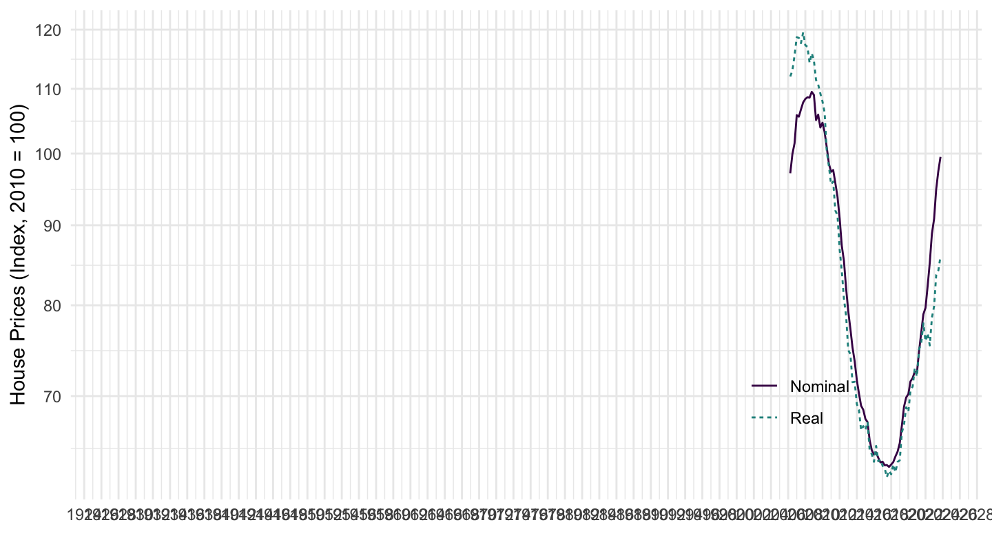
Latvia
Code
SELECTED_PP %>%
  filter(iso3c %in% c("LVA"),
         FREQ == "Q",
         UNIT_MEASURE == 628) %>%
  ggplot(.) + theme_minimal() + xlab("") + ylab("House Prices (Index, 2010 = 100)") +
  geom_line(aes(x = date, y = value, color = Value, linetype = Value)) +
  scale_x_date(breaks = seq(1900, 2100, 2) %>% paste0("-01-01") %>% as.Date,
               labels = date_format("%Y")) +
  scale_y_log10(breaks = seq(0, 600, 10),
                     labels = dollar_format(a = 1, prefix = "")) +
  scale_color_manual(values = viridis(3)[1:2]) +
  theme(legend.position = c(0.8, 0.2),
        legend.title = element_blank())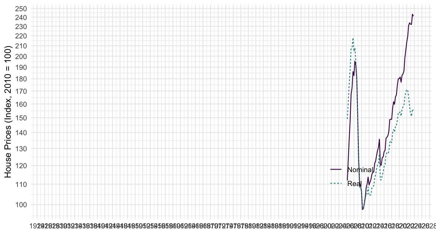
Morocco
Code
SELECTED_PP %>%
  filter(iso3c %in% c("MAR"),
         FREQ == "Q",
         UNIT_MEASURE == 628) %>%
  ggplot(.) + theme_minimal() + xlab("") + ylab("House Prices (Index, 2010 = 100)") +
  geom_line(aes(x = date, y = value, color = Value, linetype = Value)) +
  scale_x_date(breaks = seq(1900, 2100, 2) %>% paste0("-01-01") %>% as.Date,
               labels = date_format("%Y")) +
  scale_y_log10(breaks = seq(0, 600, 10),
                     labels = dollar_format(a = 1, prefix = "")) +
  scale_color_manual(values = viridis(3)[1:2]) +
  theme(legend.position = c(0.8, 0.2),
        legend.title = element_blank())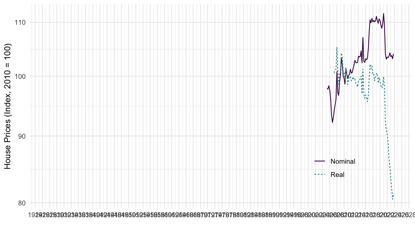
Slovak Republic
Code
SELECTED_PP %>%
  filter(iso3c %in% c("SVK"),
         FREQ == "Q",
         UNIT_MEASURE == 628) %>%
  ggplot(.) + theme_minimal() + xlab("") + ylab("House Prices (Index, 2010 = 100)") +
  geom_line(aes(x = date, y = value, color = Value, linetype = Value)) +
  scale_x_date(breaks = seq(1900, 2100, 2) %>% paste0("-01-01") %>% as.Date,
               labels = date_format("%Y")) +
  scale_y_log10(breaks = seq(0, 600, 10),
                     labels = dollar_format(a = 1, prefix = "")) +
  scale_color_manual(values = viridis(3)[1:2]) +
  theme(legend.position = c(0.8, 0.2),
        legend.title = element_blank())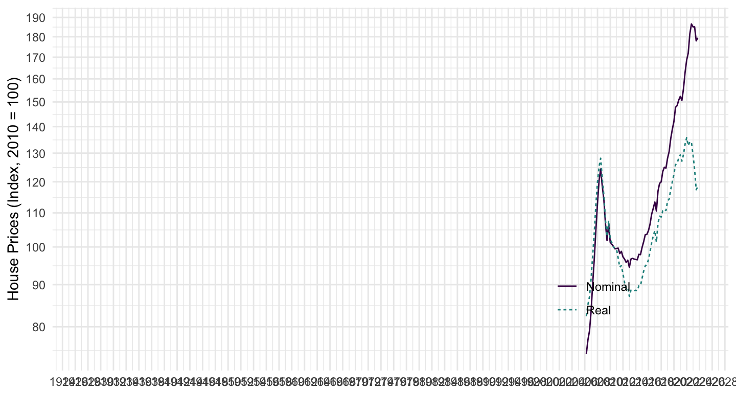
Hungary
Code
SELECTED_PP %>%
  filter(iso3c %in% c("HUN"),
         FREQ == "Q",
         UNIT_MEASURE == 628) %>%
  ggplot(.) + theme_minimal() + xlab("") + ylab("House Prices (Index, 2010 = 100)") +
  geom_line(aes(x = date, y = value, color = Value, linetype = Value)) +
  scale_x_date(breaks = seq(1900, 2100, 2) %>% paste0("-01-01") %>% as.Date,
               labels = date_format("%Y")) +
  scale_y_log10(breaks = seq(0, 600, 10),
                     labels = dollar_format(a = 1, prefix = "")) +
  scale_color_manual(values = viridis(3)[1:2]) +
  theme(legend.position = c(0.8, 0.2),
        legend.title = element_blank())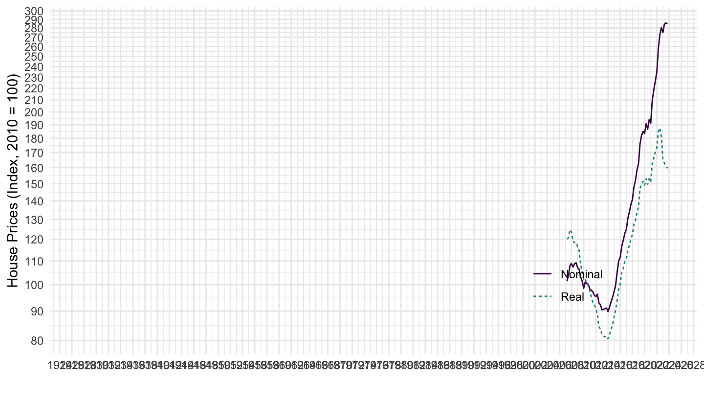
Slovenia
Code
SELECTED_PP %>%
  filter(iso3c %in% c("SVN"),
         FREQ == "Q",
         UNIT_MEASURE == 628) %>%
  ggplot(.) + theme_minimal() + xlab("") + ylab("House Prices (Index, 2010 = 100)") +
  geom_line(aes(x = date, y = value, color = Value, linetype = Value)) +
  scale_x_date(breaks = seq(1900, 2100, 2) %>% paste0("-01-01") %>% as.Date,
               labels = date_format("%Y")) +
  scale_y_log10(breaks = seq(0, 600, 10),
                     labels = dollar_format(a = 1, prefix = "")) +
  scale_color_manual(values = viridis(3)[1:2]) +
  theme(legend.position = c(0.8, 0.2),
        legend.title = element_blank())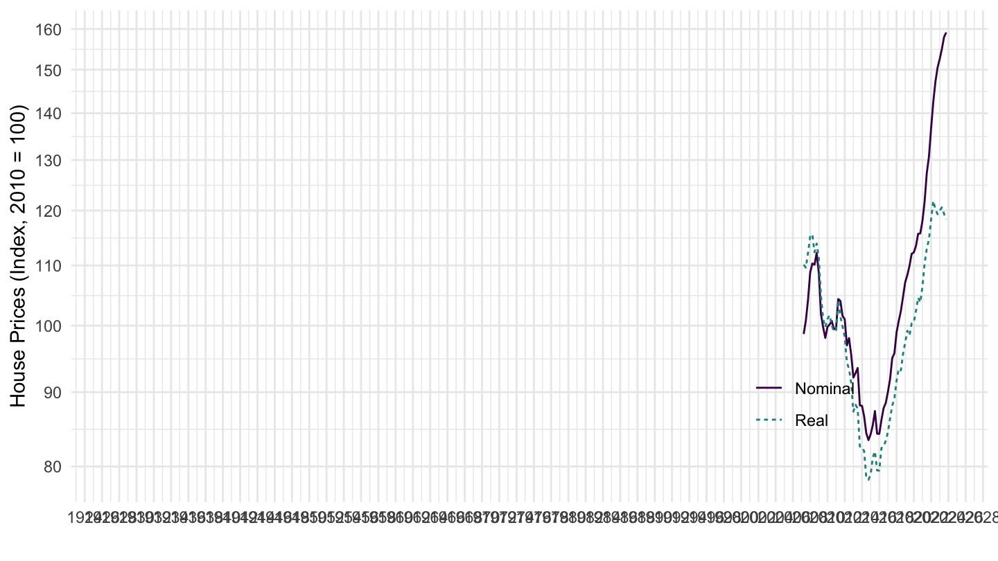
Luxembourg
Code
SELECTED_PP %>%
  filter(iso3c %in% c("LUX"),
         FREQ == "Q",
         UNIT_MEASURE == 628) %>%
  ggplot(.) + theme_minimal() + xlab("") + ylab("House Prices (Index, 2010 = 100)") +
  geom_line(aes(x = date, y = value, color = Value, linetype = Value)) +
  scale_x_date(breaks = seq(1900, 2100, 2) %>% paste0("-01-01") %>% as.Date,
               labels = date_format("%Y")) +
  scale_y_log10(breaks = seq(0, 600, 10),
                     labels = dollar_format(a = 1, prefix = "")) +
  scale_color_manual(values = viridis(3)[1:2]) +
  theme(legend.position = c(0.8, 0.2),
        legend.title = element_blank())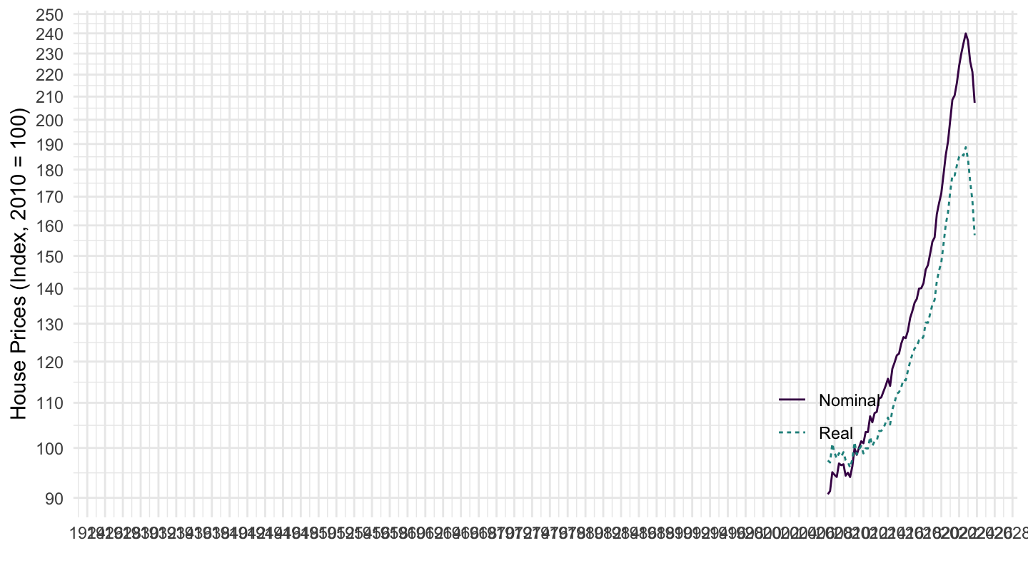
Czech Republic
Code
SELECTED_PP %>%
  filter(iso3c %in% c("CZE"),
         FREQ == "Q",
         UNIT_MEASURE == 628) %>%
  ggplot(.) + theme_minimal() + xlab("") + ylab("House Prices (Index, 2010 = 100)") +
  geom_line(aes(x = date, y = value, color = Value, linetype = Value)) +
  scale_x_date(breaks = seq(1900, 2100, 2) %>% paste0("-01-01") %>% as.Date,
               labels = date_format("%Y")) +
  scale_y_log10(breaks = seq(0, 600, 10),
                     labels = dollar_format(a = 1, prefix = "")) +
  scale_color_manual(values = viridis(3)[1:2]) +
  theme(legend.position = c(0.8, 0.2),
        legend.title = element_blank())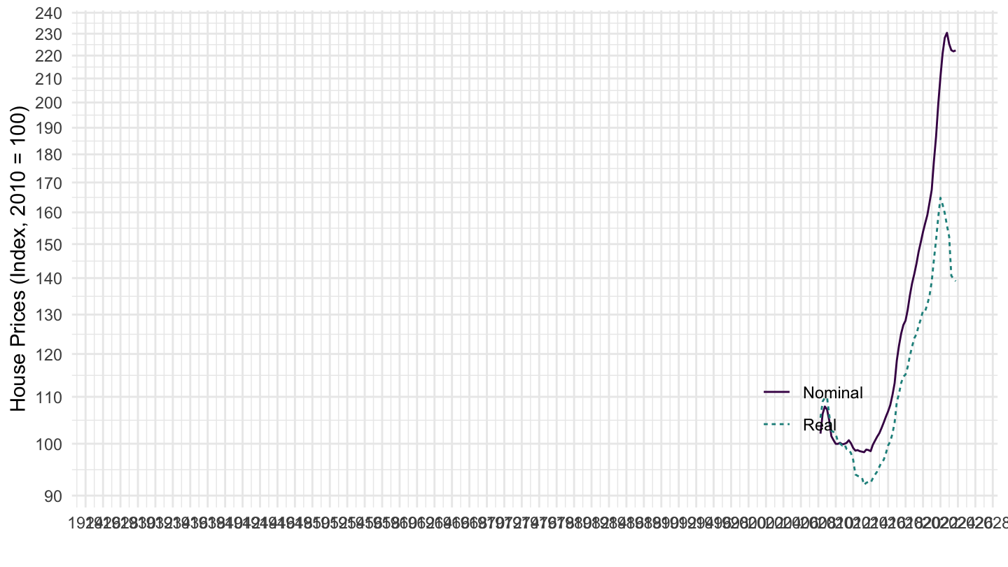
Philippines
Code
SELECTED_PP %>%
  filter(iso3c %in% c("PHL"),
         FREQ == "Q",
         UNIT_MEASURE == 628) %>%
  ggplot(.) + theme_minimal() + xlab("") + ylab("House Prices (Index, 2010 = 100)") +
  geom_line(aes(x = date, y = value, color = Value, linetype = Value)) +
  scale_x_date(breaks = seq(1900, 2100, 2) %>% paste0("-01-01") %>% as.Date,
               labels = date_format("%Y")) +
  scale_y_log10(breaks = seq(0, 600, 10),
                     labels = dollar_format(a = 1, prefix = "")) +
  scale_color_manual(values = viridis(3)[1:2]) +
  theme(legend.position = c(0.8, 0.2),
        legend.title = element_blank())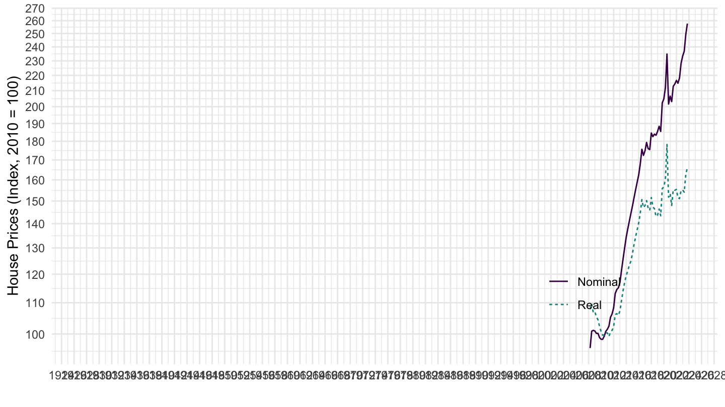
Portugal
Code
SELECTED_PP %>%
  filter(iso3c %in% c("PRT"),
         FREQ == "Q",
         UNIT_MEASURE == 628) %>%
  ggplot(.) + theme_minimal() + xlab("") + ylab("House Prices (Index, 2010 = 100)") +
  geom_line(aes(x = date, y = value, color = Value, linetype = Value)) +
  scale_x_date(breaks = seq(1900, 2100, 2) %>% paste0("-01-01") %>% as.Date,
               labels = date_format("%Y")) +
  scale_y_log10(breaks = seq(0, 600, 10),
                     labels = dollar_format(a = 1, prefix = "")) +
  scale_color_manual(values = viridis(3)[1:2]) +
  theme(legend.position = c(0.8, 0.2),
        legend.title = element_blank())
India
Code
SELECTED_PP %>%
  filter(iso3c %in% c("IND"),
         FREQ == "Q",
         UNIT_MEASURE == 628) %>%
  ggplot(.) + theme_minimal() + xlab("") + ylab("House Prices (Index, 2010 = 100)") +
  geom_line(aes(x = date, y = value, color = Value, linetype = Value)) +
  scale_x_date(breaks = seq(1900, 2100, 2) %>% paste0("-01-01") %>% as.Date,
               labels = date_format("%Y")) +
  scale_y_log10(breaks = seq(0, 600, 10),
                     labels = dollar_format(a = 1, prefix = "")) +
  scale_color_manual(values = viridis(3)[1:2]) +
  theme(legend.position = c(0.8, 0.2),
        legend.title = element_blank())
Romania
Code
SELECTED_PP %>%
  filter(iso3c %in% c("ROU"),
         FREQ == "Q",
         UNIT_MEASURE == 628) %>%
  ggplot(.) + theme_minimal() + xlab("") + ylab("House Prices (Index, 2010 = 100)") +
  geom_line(aes(x = date, y = value, color = Value, linetype = Value)) +
  scale_x_date(breaks = seq(1900, 2100, 2) %>% paste0("-01-01") %>% as.Date,
               labels = date_format("%Y")) +
  scale_y_log10(breaks = seq(0, 600, 10),
                     labels = dollar_format(a = 1, prefix = "")) +
  scale_color_manual(values = viridis(3)[1:2]) +
  theme(legend.position = c(0.8, 0.2),
        legend.title = element_blank())
Poland
Code
SELECTED_PP %>%
  filter(iso3c %in% c("POL"),
         FREQ == "Q",
         UNIT_MEASURE == 628) %>%
  ggplot(.) + theme_minimal() + xlab("") + ylab("House Prices (Index, 2010 = 100)") +
  geom_line(aes(x = date, y = value, color = Value, linetype = Value)) +
  scale_x_date(breaks = seq(1900, 2100, 2) %>% paste0("-01-01") %>% as.Date,
               labels = date_format("%Y")) +
  scale_y_log10(breaks = seq(0, 600, 10),
                     labels = dollar_format(a = 1, prefix = "")) +
  scale_color_manual(values = viridis(3)[1:2]) +
  theme(legend.position = c(0.8, 0.2),
        legend.title = element_blank())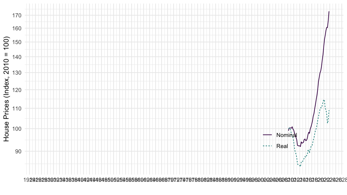
Turkey
Code
SELECTED_PP %>%
  filter(iso3c %in% c("TUR"),
         FREQ == "Q",
         UNIT_MEASURE == 628) %>%
  ggplot(.) + theme_minimal() + xlab("") + ylab("House Prices (Index, 2010 = 100)") +
  geom_line(aes(x = date, y = value, color = Value, linetype = Value)) +
  scale_x_date(breaks = seq(1900, 2100, 2) %>% paste0("-01-01") %>% as.Date,
               labels = date_format("%Y")) +
  scale_y_log10(breaks = seq(0, 600, 10),
                     labels = dollar_format(a = 1, prefix = "")) +
  scale_color_manual(values = viridis(3)[1:2]) +
  theme(legend.position = c(0.2, 0.8),
        legend.title = element_blank())