
Last observation: nov. 2025 (N = 11)
First observation: janv. 2005 (N = 9)
Last data update: 04 sept. 2026, 12:17
Last compile: 10 oct. 2026, 01:18
`IPGD-2015` |>
  filter(`FORME-VENTE` == "GD",
         PRIX_CONSO %in% c("PROD_GC", "PA-TOTAL"),
         NATURE == "INDICE") |>
  month_to_date() |>
  filter(date >= as.Date("2017-01-01")) |>

  group_by(`Prix_conso`) |>
  arrange(date) |>
  mutate(OBS_VALUE = 100*OBS_VALUE/OBS_VALUE[1]) |>
  ggplot() + geom_line(aes(x = date, y = OBS_VALUE, color = Prix_conso)) +
  theme_minimal() + xlab("") + ylab("Augmentation vs. Janvier 2017") +
  theme(legend.position = c(0.2, 0.8),
        legend.title = element_blank(),
        axis.text.x = element_text(angle = 45, vjust = 0.5, hjust=1)) +
  scale_y_continuous(breaks = seq(-100, 500, 2),
                     labels = percent(seq(-100, 500, 2)/100-1)) +
  scale_x_date(breaks = seq.Date(as.Date("2017-01-01"), Sys.Date(), by = "6 months"),
               labels = date_format("%B %Y"))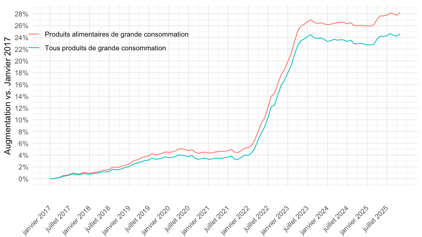
`IPGD-2015` |>
  filter(`FORME-VENTE` == "GD",
         PRIX_CONSO %in% c("PROD_GC", "PA-TOTAL"),
         NATURE == "INDICE") |>
  month_to_date() |>
  filter(date >= as.Date("2021-10-01")) |>

  group_by(`Prix_conso`) |>
  arrange(date) |>
  mutate(OBS_VALUE = 100*OBS_VALUE/OBS_VALUE[1]) |>
  ggplot() + geom_line(aes(x = date, y = OBS_VALUE, color = Prix_conso)) +
  theme_minimal() + xlab("") + ylab("Augmentation vs. Octobre 2021") +
  theme(legend.position = c(0.6, 0.2),
        legend.title = element_blank(),
        axis.text.x = element_text(angle = 45, vjust = 0.5, hjust=1)) +
  scale_y_continuous(breaks = seq(-100, 500, 2),
                     labels = percent(seq(-100, 500, 2)/100-1)) +
  scale_x_date(breaks = "2 months",
               labels = date_format("%b %Y"))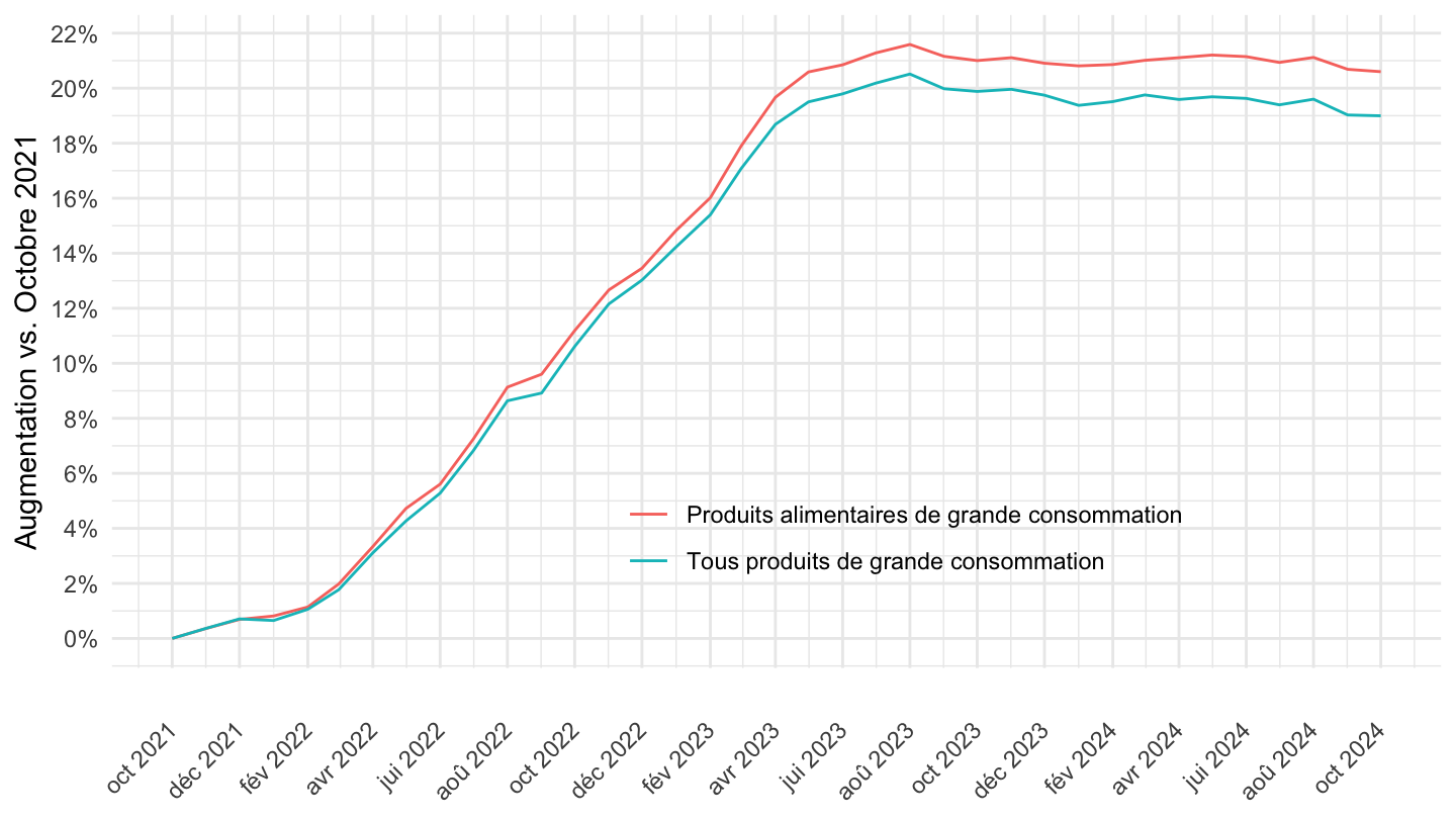
`IPGD-2015` |>
  filter(PRIX_CONSO %in% c("PA-TOTAL", "PA-BOISSON", "PA-VIANDES", "PEH-TOTAL")) |>
  month_to_date() |>

  ggplot() + geom_line(aes(x = date, y = OBS_VALUE, color = Prix_conso)) +
  theme_minimal() + xlab("") + ylab("") +
  theme(legend.position = c(0.3, 0.8),
        legend.title = element_blank()) +
  scale_y_continuous(breaks = seq(-100, 500, 5)) +
  scale_x_date(breaks = seq(1920, 2100, 2) |> paste0("-01-01") |> as.Date(),
               labels = date_format("%Y"))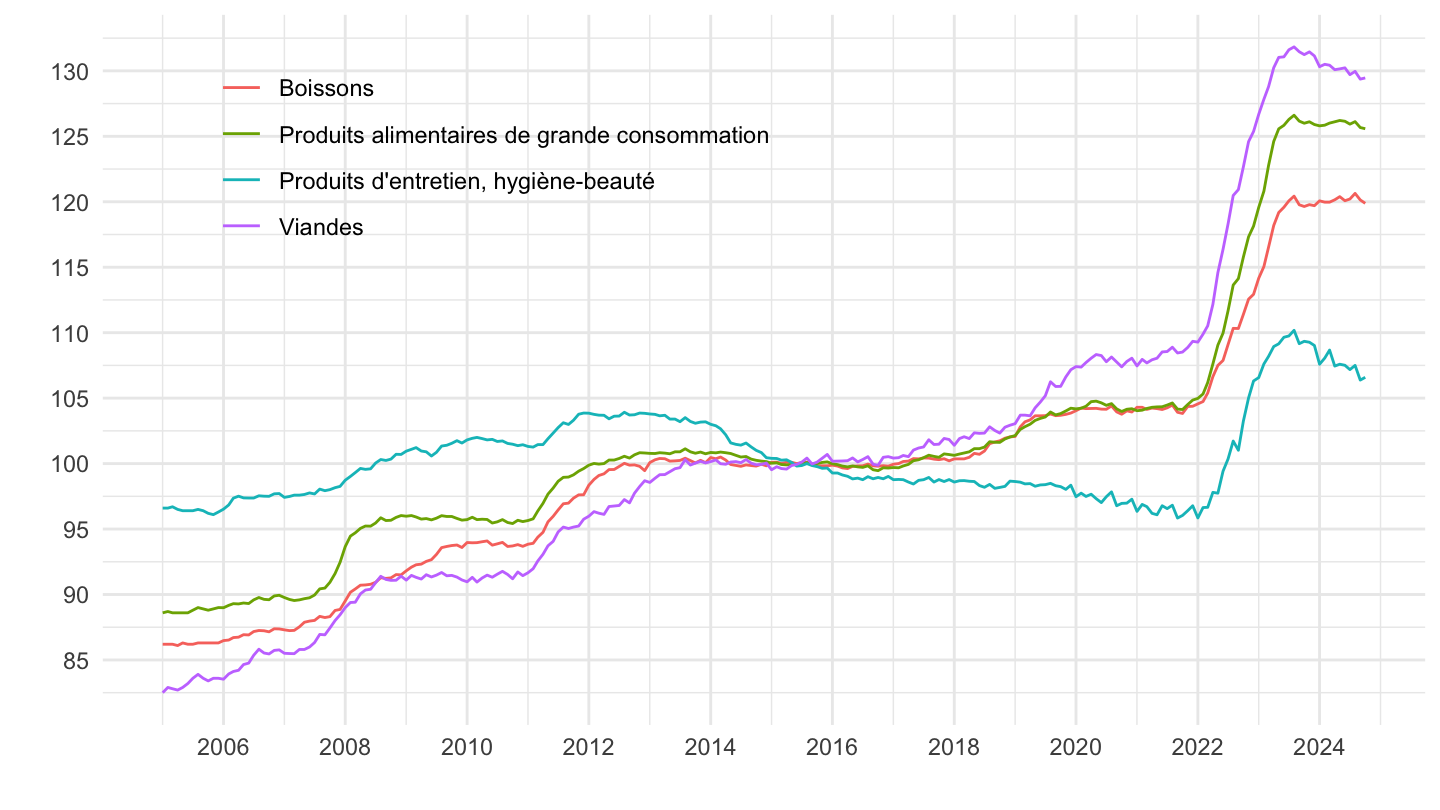
`IPGD-2015` |>
  filter(`FORME-VENTE` == "GD",
         PRIX_CONSO %in% c("PA-TOTAL", "PA-VIANDES", "PEH-TOTAL", "PROD_GC"),
         NATURE == "INDICE") |>
  month_to_date() |>
  filter(date >= as.Date("2017-01-01")) |>

  group_by(Prix_conso) |>
  arrange(date) |>
  mutate(OBS_VALUE = 100*OBS_VALUE/OBS_VALUE[1]) |>
  ggplot() + geom_line(aes(x = date, y = OBS_VALUE, color = Prix_conso, linetype = Prix_conso)) +
  scale_linetype_manual(values = c("solid", "dashed","solid","dashed")) +
  scale_color_manual(values = c("forestgreen", "orange","black","maroon")) +
  theme_minimal() + xlab("") + ylab("Augmentation vs. Janvier 2017") +
  theme(legend.position = c(0.35, 0.8),
        legend.title = element_blank(),
        axis.text.x = element_text(angle = 45, vjust = 0.5, hjust=1)) +
  scale_y_continuous(breaks = seq(-100, 500, 2),
                     labels = percent(seq(-100, 500, 2)/100-1)) +
  scale_x_date(breaks = seq.Date(as.Date("2017-01-01"), Sys.Date(), by = "6 months"),
               labels = date_format("%B %Y"))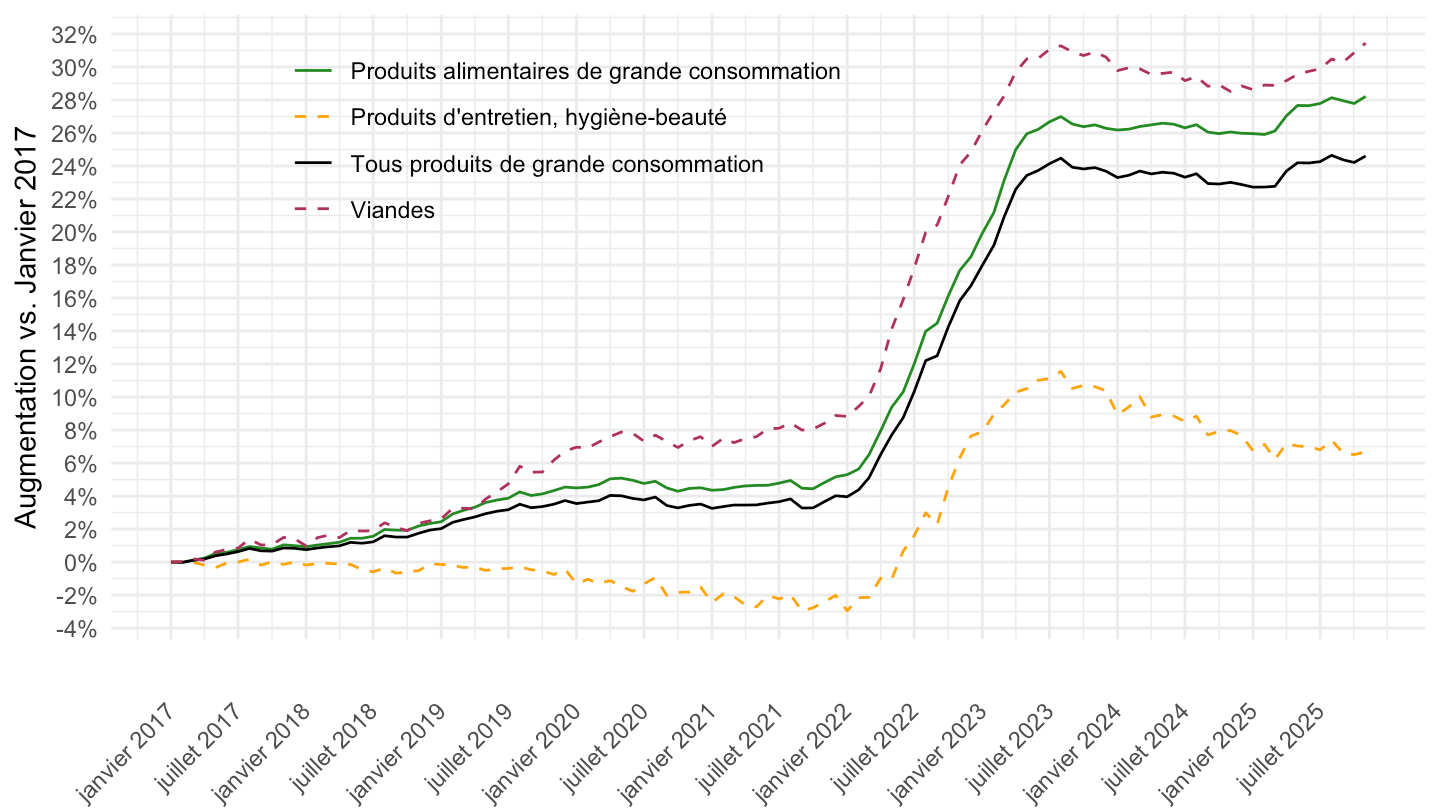
`IPGD-2015` |>
  filter(`FORME-VENTE` == "GD",
         PRIX_CONSO %in% c("PA-TOTAL", "PA-VIANDES", "PEH-TOTAL", "PROD_GC"),
         NATURE == "INDICE") |>
  month_to_date() |>
  filter(date >= as.Date("2021-04-01")) |>

  group_by(Prix_conso) |>
  arrange(date) |>
  mutate(OBS_VALUE = 100*OBS_VALUE/OBS_VALUE[1]) |>
  ggplot() + geom_line(aes(x = date, y = OBS_VALUE, color = Prix_conso, linetype = Prix_conso)) +
  scale_linetype_manual(values = c("solid", "dashed","solid","dashed")) +
  scale_color_manual(values = c("forestgreen", "orange","black","maroon")) +
  theme_minimal() + xlab("") + ylab("Augmentation vs. Avril 2021") +
  theme(legend.position = c(0.25, 0.8),
        legend.title = element_blank(),
        axis.text.x = element_text(angle = 45, vjust = 0.5, hjust=1)) +
  scale_y_continuous(breaks = seq(-100, 500, 2),
                     labels = percent(seq(-100, 500, 2)/100-1)) +
  scale_x_date(breaks = "2 months",
               labels = date_format("%b %Y"))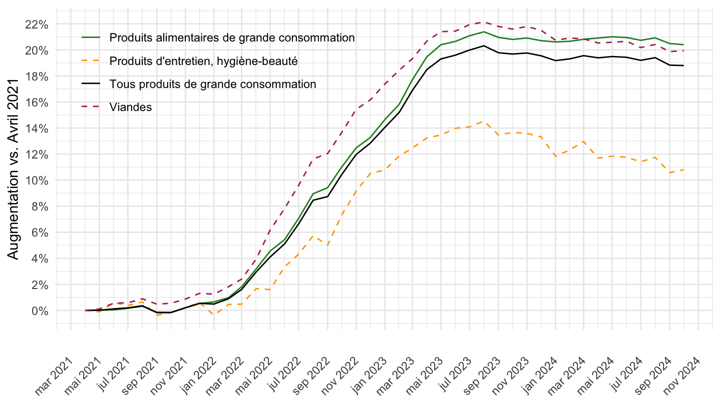
`IPGD-2015` |>
  filter(PRIX_CONSO %in% c("PA-TOTAL", "PA-BOISSON", "PA-VIANDES", "PEH-TOTAL")) |>
  month_to_date() |>
  filter(date >= as.Date("2022-01-01")) |>

  group_by(Prix_conso) |>
  arrange(date) |>
  mutate(OBS_VALUE = 100*OBS_VALUE/OBS_VALUE[1]) |>
  ggplot() + geom_line(aes(x = date, y = OBS_VALUE, color = Prix_conso)) +
  theme_minimal() + xlab("") + ylab("") +
  theme(legend.position = c(0.25, 0.8),
        legend.title = element_blank(),
        axis.text.x = element_text(angle = 45, vjust = 0.5, hjust=1)) +
  scale_y_continuous(breaks = seq(-100, 500, 2)) +
  scale_x_date(breaks = "2 months",
               labels = date_format("%b %Y"))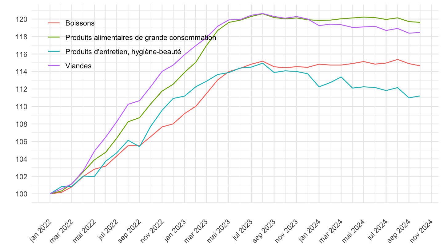
`IPGD-2015` |>
  filter(PRIX_CONSO %in% c("PROD_GC"),
         NATURE == "INDICE") |>
  month_to_date() |>
  filter(date >= as.Date("2017-01-01")) |>

  group_by(`Forme-Vente`) |>
  arrange(date) |>
  mutate(OBS_VALUE = 100*OBS_VALUE/OBS_VALUE[1]) |>
  ggplot() + geom_line(aes(x = date, y = OBS_VALUE, color = `Forme-Vente`)) +
  theme_minimal() + xlab("") + ylab("Augmentation vs. Janvier 2017") +
  theme(legend.position = c(0.2, 0.8),
        legend.title = element_blank(),
        axis.text.x = element_text(angle = 45, vjust = 0.5, hjust=1)) +
  scale_y_continuous(breaks = seq(-100, 500, 2),
                     labels = percent(seq(-100, 500, 2)/100-1)) +
  scale_x_date(breaks = seq.Date(as.Date("2017-01-01"), Sys.Date(), by = "6 months"),
               labels = date_format("%B %Y"))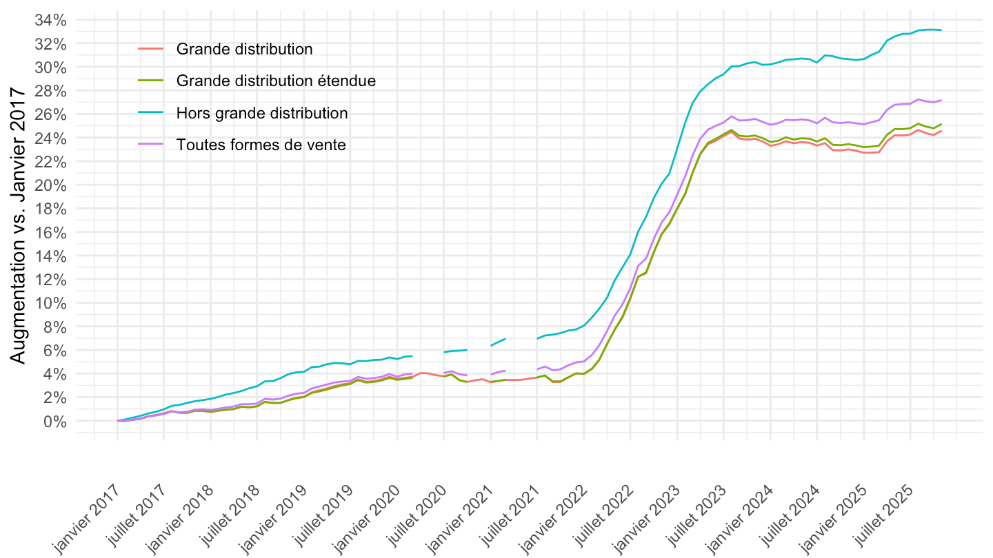
`IPGD-2015` |>
  filter(PRIX_CONSO %in% c("PROD_GC"),
         NATURE == "INDICE") |>
  month_to_date() |>
  filter(date >= as.Date("2021-11-01")) |>

  group_by(`Forme-Vente`) |>
  arrange(date) |>
  mutate(OBS_VALUE = 100*OBS_VALUE/OBS_VALUE[1]) |>
  ggplot() + geom_line(aes(x = date, y = OBS_VALUE, color = `Forme-Vente`)) +
  theme_minimal() + xlab("") + ylab("Augmentation vs. Novembre 2021") +
  theme(legend.position = c(0.2, 0.8),
        legend.title = element_blank(),
        axis.text.x = element_text(angle = 45, vjust = 0.5, hjust=1)) +
  scale_y_continuous(breaks = seq(-100, 500, 2),
                     labels = percent(seq(-100, 500, 2)/100-1)) +
  scale_x_date(breaks = seq.Date(as.Date("2021-11-01"), Sys.Date(), by = "3 months"),
               labels = date_format("%B %Y"))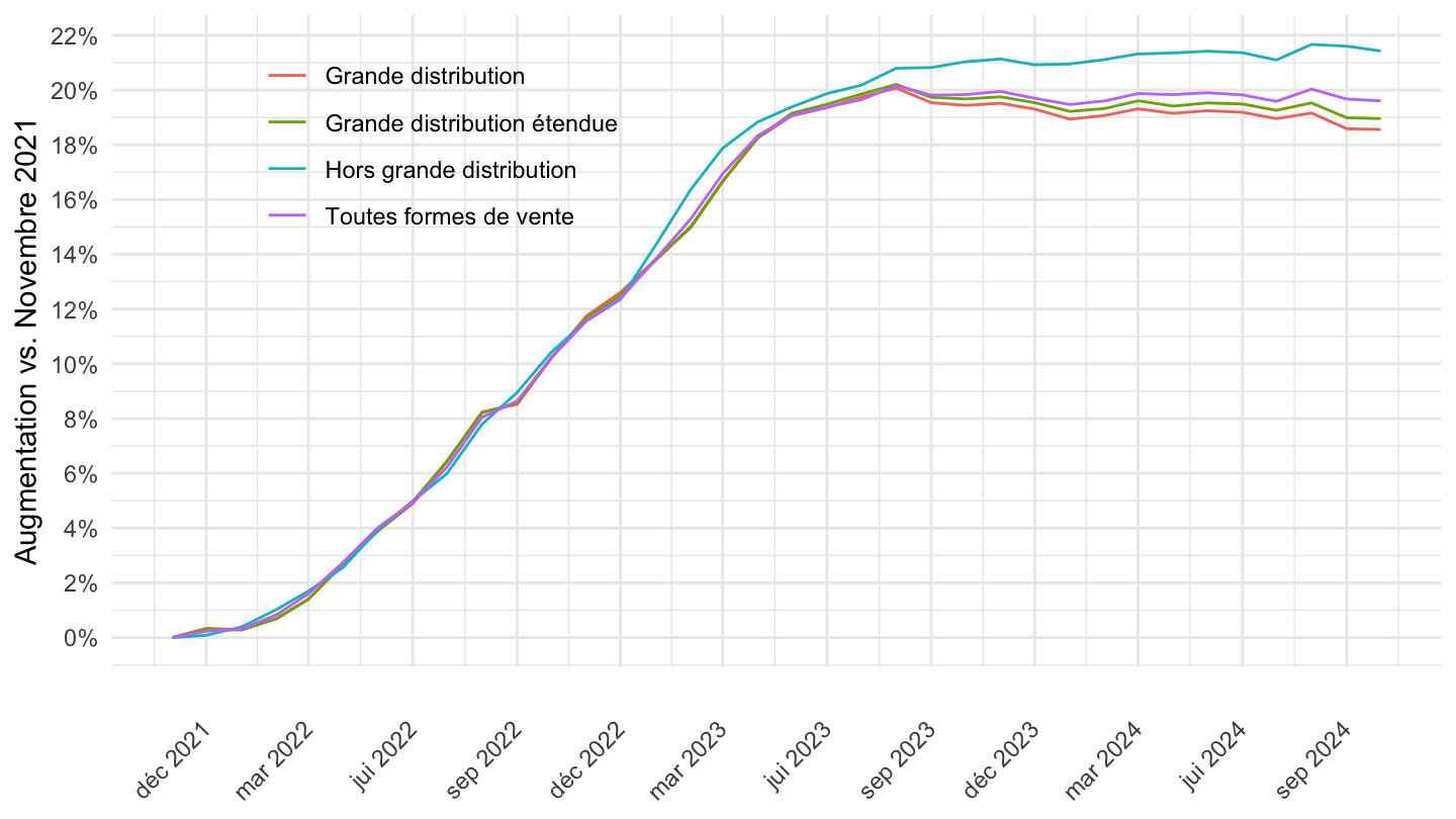
| source | dataset | Title | Updated |
|---|---|---|---|
| source | dataset | Title | Updated |
|---|---|---|---|
