Indices des prix à la consommation harmonisés
Données - INSEE
Info
Données sur l’inflation en France
| Title | source | dataset | .html | .RData |
|---|---|---|---|---|
| Budget de famille 2017 | insee | bdf2017 | 2026-07-24 | 2023-11-21 |
| Échantillon d’agglomérations enquêtées de l’IPC en 2024 | insee | echantillon-agglomerations-IPC-2024 | 2026-07-24 | 2026-01-27 |
| Échantillon d’agglomérations enquêtées de l’IPC en 2025 | insee | echantillon-agglomerations-IPC-2025 | 2026-07-24 | 2026-01-27 |
| Indices pour la révision d’un bail commercial ou professionnel | insee | ILC-ILAT-ICC | 2026-07-24 | NA |
| Indices des loyers d'habitation (ILH) | insee | INDICES_LOYERS | 2026-07-24 | 2026-07-24 |
| Indice des prix à la consommation - Base 1970, 1980 | insee | IPC-1970-1980 | 2026-07-24 | NA |
| Indices des prix à la consommation - Base 1990 | insee | IPC-1990 | 2026-07-24 | NA |
| Indice des prix à la consommation - Base 2015 | insee | IPC-2015 | 2026-07-24 | 2026-07-23 |
| Prix moyens de vente de détail | insee | IPC-PM-2015 | 2026-07-24 | NA |
| Indices des prix à la consommation harmonisés | insee | IPCH-2015 | 2026-07-24 | 2026-07-24 |
| Indices des prix à la consommation harmonisés | insee | IPCH-IPC-2015-ensemble | 2026-07-23 | 2026-07-24 |
| Indice des prix dans la grande distribution | insee | IPGD-2015 | 2026-07-24 | NA |
| Indices des prix des logements neufs et Indices Notaires-Insee des prix des logements anciens | insee | IPLA-IPLNA-2015 | 2026-07-24 | NA |
| Indices de prix de production et d'importation dans l'industrie | insee | IPPI-2015 | 2026-07-24 | NA |
| Indice pour la révision d’un loyer d’habitation | insee | IRL | 2026-07-24 | 2026-07-23 |
| Liste des variétés pour la mesure de l'IPC en 2024 | insee | liste-varietes-IPC-2024 | 2026-07-23 | 2025-04-02 |
| Liste des variétés pour la mesure de l'IPC en 2025 | insee | liste-varietes-IPC-2025 | 2026-07-23 | 2026-01-27 |
| Pondérations élémentaires 2024 intervenant dans le calcul de l’IPC | insee | ponderations-elementaires-IPC-2024 | 2026-07-23 | 2025-04-02 |
| Pondérations élémentaires 2025 intervenant dans le calcul de l’IPC | insee | ponderations-elementaires-IPC-2025 | 2026-07-23 | 2026-01-27 |
| Variation des loyers | insee | SERIES_LOYERS | 2026-07-23 | 2026-07-23 |
| Consommation effective des ménages par fonction | insee | T_CONSO_EFF_FONCTION | 2026-07-23 | 2025-12-22 |
| Montants de consommation selon différentes catégories de ménages | insee | table_conso_moyenne_par_categorie_menages | 2026-07-23 | 2026-01-27 |
| Ventilation de chaque sous-classe (niveau 4 de la COICOP v2) en postes et leurs pondérations | insee | table_poste_au_sein_sous_classe_ecoicopv2_france_entiere_ | 2026-07-23 | 2026-01-27 |
| Poids de chaque tranche d’unités urbaines dans la consommation | insee | tranches_unitesurbaines | 2026-07-23 | 2026-01-27 |
LAST_COMPILE
| LAST_COMPILE |
|---|
| 2026-07-24 |
IPC vs IPCH
Annuel
1996-
Code
`IPCH-IPC-2015-ensemble-A` %>%
  filter(date >= zoo::as.Date("1996-01-01")) %>%
  arrange(date) %>%
  group_by(INDICATEUR) %>%
  mutate(OBS_VALUE = 100*OBS_VALUE/OBS_VALUE[1]) %>%
  ggplot + geom_line(aes(x = date, y = OBS_VALUE, color = INDICATEUR)) +
  xlab("") + ylab("") + theme_minimal() +
  theme(legend.title = element_blank(),
        legend.position = c(0.3, 0.9)) +
  scale_x_date(breaks = seq(1920, 2100, 2) %>% paste0("-01-01") %>% as.Date(),
               labels = date_format("%Y")) +
  scale_y_log10(breaks = seq(0, 1000, 10)) +
  geom_label_repel(data = . %>% filter(date == max(date)),
             aes(x = date, y = OBS_VALUE, color = INDICATEUR, label = round(OBS_VALUE, 1)),
             show.legend = F)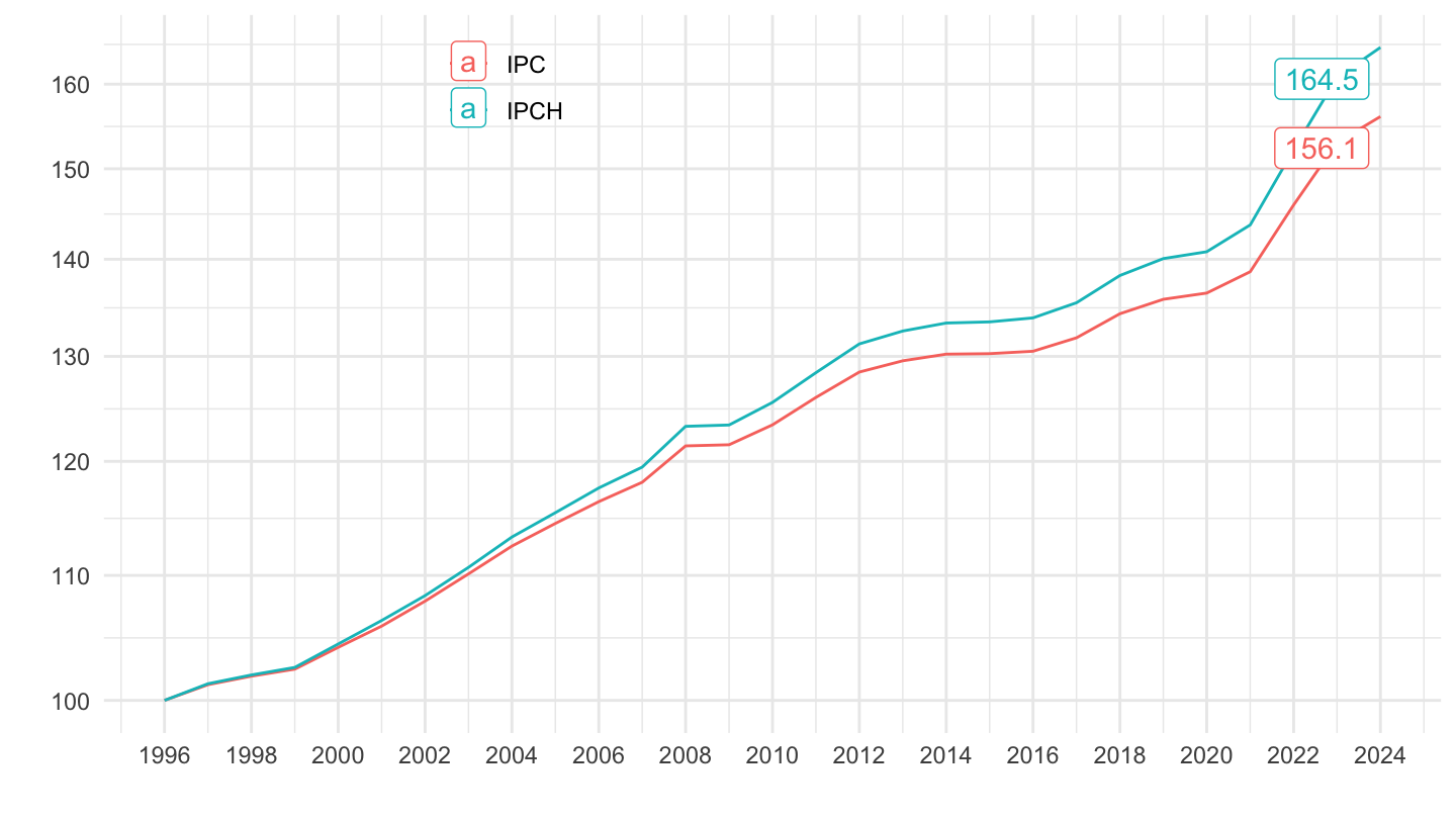
1999-
Code
`IPCH-IPC-2015-ensemble-A` %>%
  filter(date >= zoo::as.Date("1999-01-01")) %>%
  arrange(date) %>%
  group_by(INDICATEUR) %>%
  mutate(OBS_VALUE = 100*OBS_VALUE/OBS_VALUE[1]) %>%
  ggplot + geom_line(aes(x = date, y = OBS_VALUE, color = INDICATEUR)) +
  xlab("") + ylab("") + theme_minimal() +
  theme(legend.title = element_blank(),
        legend.position = c(0.3, 0.9)) +
  scale_x_date(breaks = seq(1920, 2100, 2) %>% paste0("-01-01") %>% as.Date(),
               labels = date_format("%Y")) +
  scale_y_log10(breaks = seq(0, 1000, 10)) +
  geom_label_repel(data = . %>% filter(date == max(date)),
             aes(x = date, y = OBS_VALUE, color = INDICATEUR, label = round(OBS_VALUE, 1)),
             show.legend = F)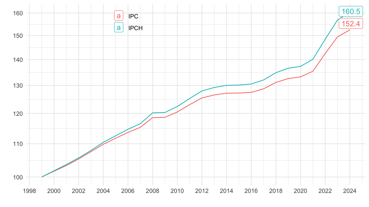
2008-
Code
`IPCH-IPC-2015-ensemble-A` %>%
  filter(date >= zoo::as.Date("2008-01-01")) %>%
  arrange(date) %>%
  group_by(INDICATEUR) %>%
  mutate(OBS_VALUE = 100*OBS_VALUE/OBS_VALUE[1]) %>%
  ggplot + geom_line(aes(x = date, y = OBS_VALUE, color = INDICATEUR)) +
  xlab("") + ylab("") + theme_minimal() +
  theme(legend.title = element_blank(),
        legend.position = c(0.3, 0.9)) +
  scale_x_date(breaks = seq(1920, 2100, 1) %>% paste0("-01-01") %>% as.Date(),
               labels = date_format("%Y")) +
  scale_y_log10(breaks = seq(0, 1000, 5)) +
  geom_label_repel(data = . %>% filter(date == max(date)),
             aes(x = date, y = OBS_VALUE, color = INDICATEUR, label = round(OBS_VALUE, 1)),
             show.legend = F)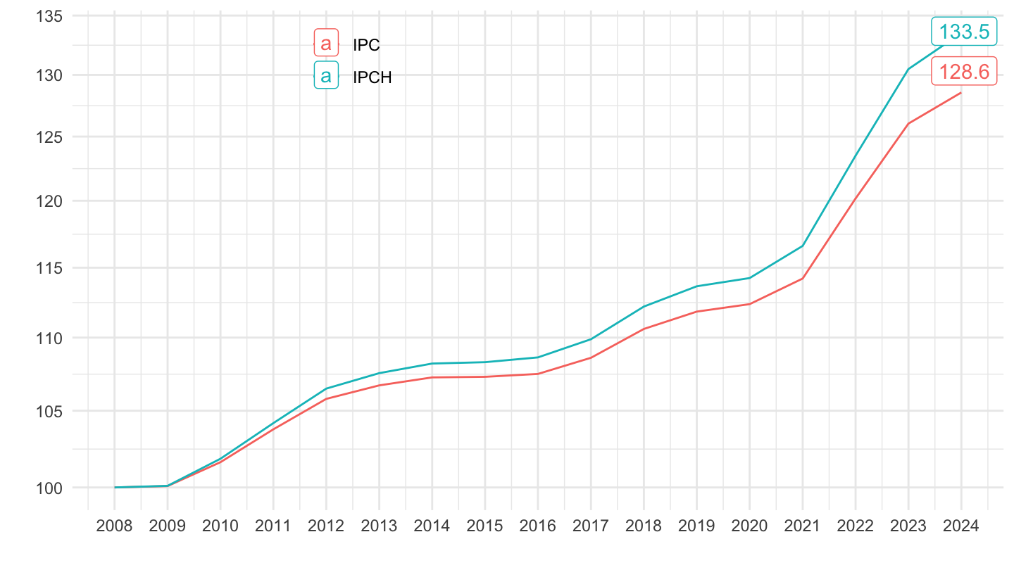
2017-
Code
`IPCH-IPC-2015-ensemble-A` %>%
  filter(date >= zoo::as.Date("2017-01-01")) %>%
  arrange(date) %>%
  group_by(INDICATEUR) %>%
  mutate(OBS_VALUE = 100*OBS_VALUE/OBS_VALUE[1]) %>%
  ggplot + geom_line(aes(x = date, y = OBS_VALUE, color = INDICATEUR)) +
  xlab("") + ylab("") + theme_minimal() +
  theme(legend.title = element_blank(),
        legend.position = c(0.3, 0.9)) +
  scale_x_date(breaks = seq(1920, 2100, 1) %>% paste0("-01-01") %>% as.Date(),
               labels = date_format("%Y")) +
  scale_y_log10(breaks = seq(0, 1000, 5)) +
  geom_label_repel(data = . %>% filter(date == max(date)),
             aes(x = date, y = OBS_VALUE, color = INDICATEUR, label = round(OBS_VALUE, 1)),
             show.legend = F)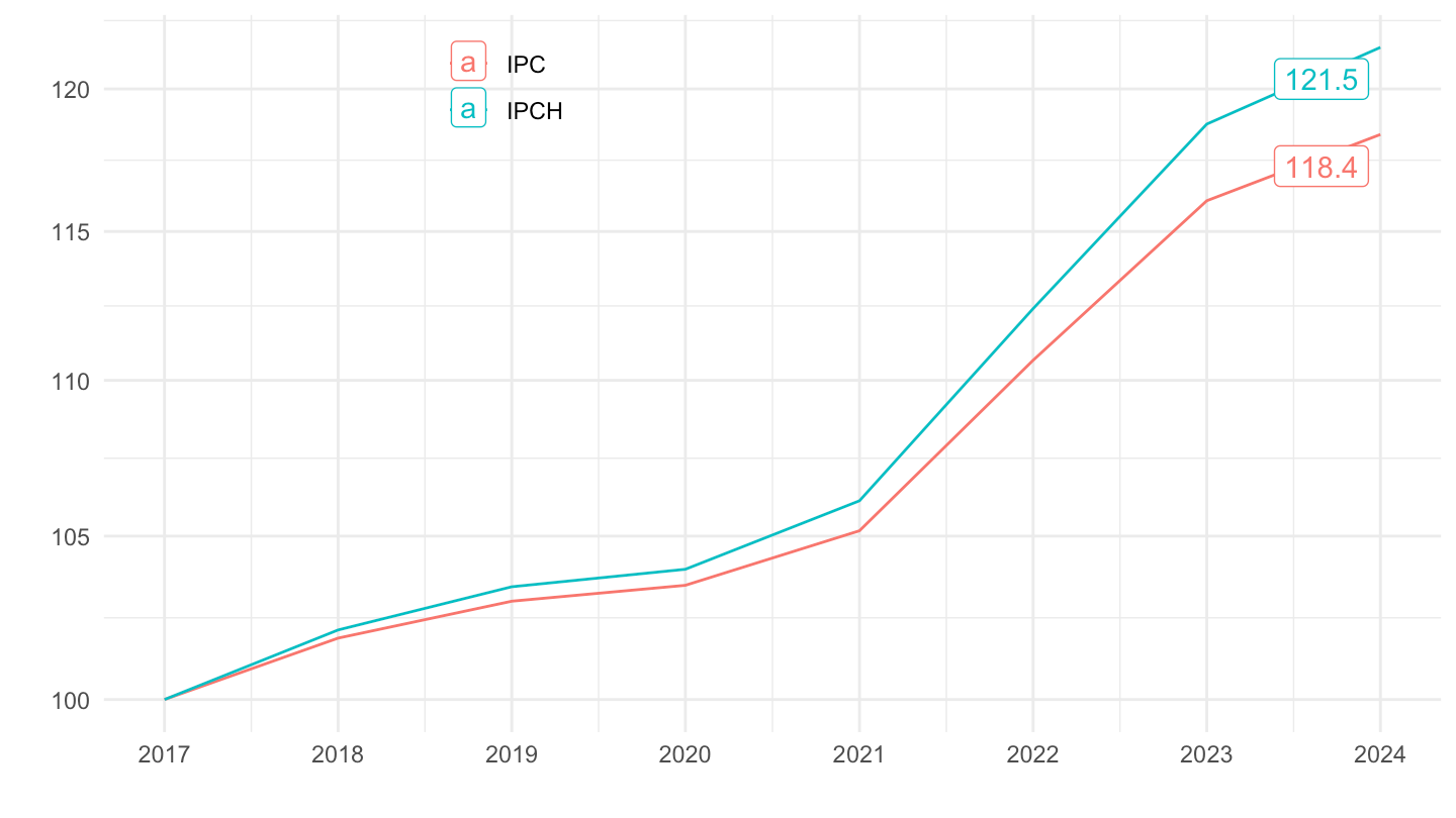
2020-
Code
`IPCH-IPC-2015-ensemble-A` %>%
  filter(date >= zoo::as.Date("2020-01-01")) %>%
  arrange(date) %>%
  group_by(INDICATEUR) %>%
  mutate(OBS_VALUE = 100*OBS_VALUE/OBS_VALUE[1]) %>%
  ggplot + geom_line(aes(x = date, y = OBS_VALUE, color = INDICATEUR)) +
  xlab("") + ylab("") + theme_minimal() +
  theme(legend.title = element_blank(),
        legend.position = c(0.3, 0.9)) +
  scale_x_date(breaks = seq(1920, 2100, 1) %>% paste0("-01-01") %>% as.Date(),
               labels = date_format("%Y")) +
  scale_y_log10(breaks = seq(0, 1000, 5)) +
  geom_label_repel(data = . %>% filter(date == max(date)),
             aes(x = date, y = OBS_VALUE, color = INDICATEUR, label = round(OBS_VALUE, 1)),
             show.legend = F)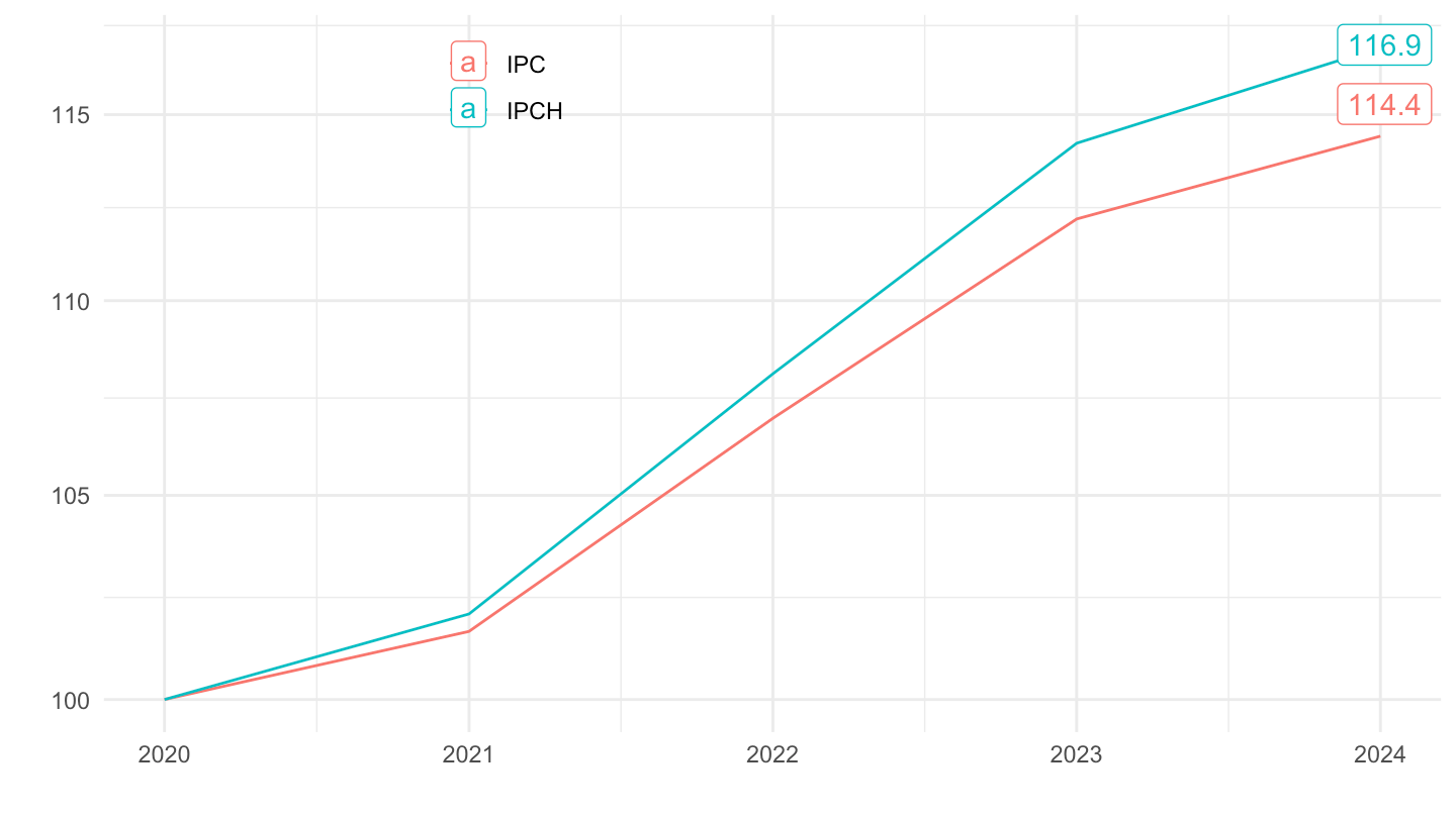
Trimestriel
1996-
Code
`IPCH-IPC-2015-ensemble-Q` %>%
  filter(date >= zoo::as.yearqtr("1996 Q1")) %>%
  arrange(date) %>%
  group_by(INDICATEUR) %>%
  mutate(OBS_VALUE = 100*OBS_VALUE/OBS_VALUE[1]) %>%
  ggplot + geom_line(aes(x = date, y = OBS_VALUE, color = INDICATEUR)) +
  xlab("") + ylab("") + theme_minimal() +
  theme(legend.title = element_blank(),
        legend.position = c(0.3, 0.9),
        axis.text.x = element_text(angle = 45, vjust = 1, hjust = 1)) +
  scale_x_yearqtr(labels = date_format("%YT%q"),
                  breaks = expand.grid(seq(1996, 2100, 2), c(1)) %>%
                         mutate(breaks = zoo::as.yearqtr(paste0(Var1, "Q", Var2))) %>%
                         pull(breaks)) +
  scale_y_log10(breaks = seq(0, 1000, 10)) +
  geom_label(data = . %>% filter(date == max(date)),
             aes(x = date, y = OBS_VALUE, color = INDICATEUR, label = round(OBS_VALUE, 1)),
             show.legend = F)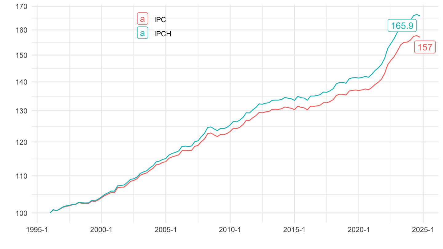
1999-
Code
`IPCH-IPC-2015-ensemble-Q` %>%
  filter(date >= zoo::as.yearqtr("1999 Q1")) %>%
  arrange(date) %>%
  group_by(INDICATEUR) %>%
  mutate(OBS_VALUE = 100*OBS_VALUE/OBS_VALUE[1]) %>%
  ggplot + geom_line(aes(x = date, y = OBS_VALUE, color = INDICATEUR)) +
  xlab("") + ylab("") + theme_minimal() +
  theme(legend.title = element_blank(),
        legend.position = c(0.3, 0.9),
        axis.text.x = element_text(angle = 45, vjust = 1, hjust = 1)) +
  scale_x_yearqtr(labels = date_format("%YT%q"),
                  breaks = expand.grid(seq(1999, 2100, 2), c(1)) %>%
                         mutate(breaks = zoo::as.yearqtr(paste0(Var1, "Q", Var2))) %>%
                         pull(breaks)) +
  scale_y_log10(breaks = seq(0, 1000, 10)) +
  geom_label(data = . %>% filter(date == max(date)),
             aes(x = date, y = OBS_VALUE, color = INDICATEUR, label = round(OBS_VALUE, 1)),
             show.legend = F)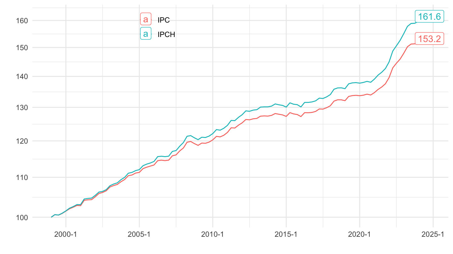
2001-
Code
`IPCH-IPC-2015-ensemble-Q` %>%
  filter(date >= zoo::as.yearqtr("2001 Q1")) %>%
  arrange(date) %>%
  group_by(INDICATEUR) %>%
  mutate(OBS_VALUE = 100*OBS_VALUE/OBS_VALUE[1]) %>%
  ggplot + geom_line(aes(x = date, y = OBS_VALUE, color = INDICATEUR)) +
  xlab("") + ylab("") + theme_minimal() +
  theme(legend.title = element_blank(),
        legend.position = c(0.3, 0.9),
        axis.text.x = element_text(angle = 45, vjust = 1, hjust = 1)) +
  scale_x_yearqtr(labels = date_format("%YT%q"),
                  breaks = expand.grid(seq(1999, 2100, 2), c(1)) %>%
                         mutate(breaks = zoo::as.yearqtr(paste0(Var1, "Q", Var2))) %>%
                         pull(breaks)) +
  scale_y_log10(breaks = seq(0, 1000, 10)) +
  geom_label(data = . %>% filter(date == max(date)),
             aes(x = date, y = OBS_VALUE, color = INDICATEUR, label = round(OBS_VALUE, 1)),
             show.legend = F)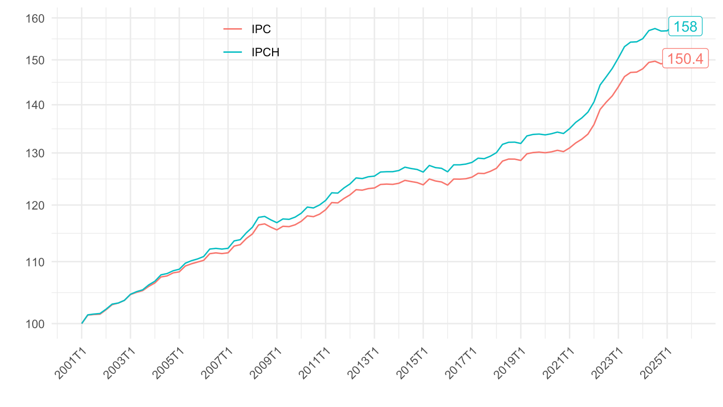
2001-2021
Code
`IPCH-IPC-2015-ensemble-Q` %>%
  filter(date >= zoo::as.yearqtr("2001 Q1"),
         date <= zoo::as.yearqtr("2021 Q1")) %>%
  arrange(date) %>%
  group_by(INDICATEUR) %>%
  mutate(OBS_VALUE = 100*OBS_VALUE/OBS_VALUE[1]) %>%
  ggplot + geom_line(aes(x = date, y = OBS_VALUE, color = INDICATEUR)) +
  xlab("") + ylab("") + theme_minimal() +
  theme(legend.title = element_blank(),
        legend.position = c(0.3, 0.9),
        axis.text.x = element_text(angle = 45, vjust = 1, hjust = 1)) +
  scale_x_yearqtr(labels = date_format("%YT%q"),
                  breaks = expand.grid(seq(1999, 2100, 2), c(1)) %>%
                         mutate(breaks = zoo::as.yearqtr(paste0(Var1, "Q", Var2))) %>%
                         pull(breaks)) +
  scale_y_log10(breaks = seq(0, 1000, 10)) +
  geom_label(data = . %>% filter(date == max(date)),
             aes(x = date, y = OBS_VALUE, color = INDICATEUR, label = round(OBS_VALUE, 1)),
             show.legend = F)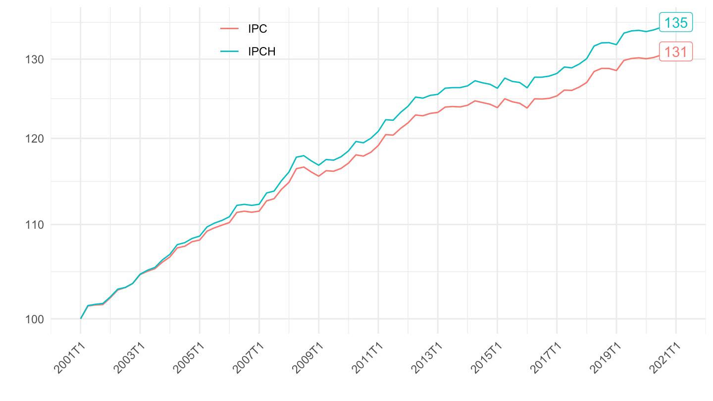
2001-2024
Code
`IPCH-IPC-2015-ensemble-Q` %>%
  filter(date >= zoo::as.yearqtr("2001 Q1"),
         date <= zoo::as.yearqtr("2024 Q1")) %>%
  arrange(date) %>%
  group_by(INDICATEUR) %>%
  mutate(OBS_VALUE = 100*OBS_VALUE/OBS_VALUE[1]) %>%
  ggplot + geom_line(aes(x = date, y = OBS_VALUE, color = INDICATEUR)) +
  xlab("") + ylab("") + theme_minimal() +
  theme(legend.title = element_blank(),
        legend.position = c(0.3, 0.9),
        axis.text.x = element_text(angle = 45, vjust = 1, hjust = 1)) +
  scale_x_yearqtr(labels = date_format("%YT%q"),
                  breaks = expand.grid(seq(1999, 2100, 2), c(1)) %>%
                         mutate(breaks = zoo::as.yearqtr(paste0(Var1, "Q", Var2))) %>%
                         pull(breaks)) +
  scale_y_log10(breaks = seq(0, 1000, 10)) +
  geom_label(data = . %>% filter(date == max(date)),
             aes(x = date, y = OBS_VALUE, color = INDICATEUR, label = round(OBS_VALUE, 1)),
             show.legend = F)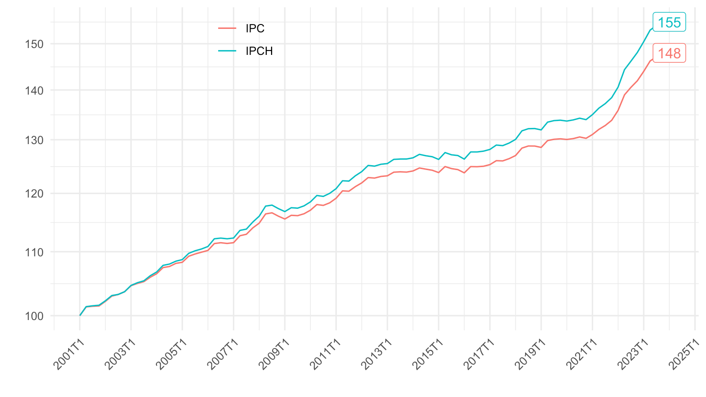
2008-
Code
`IPCH-IPC-2015-ensemble-Q` %>%
  filter(date >= zoo::as.yearqtr("2008 Q1")) %>%
  arrange(date) %>%
  group_by(INDICATEUR) %>%
  mutate(OBS_VALUE = 100*OBS_VALUE/OBS_VALUE[1]) %>%
  ggplot + geom_line(aes(x = date, y = OBS_VALUE, color = INDICATEUR)) +
  xlab("") + ylab("") + theme_minimal() +
  theme(legend.title = element_blank(),
        legend.position = c(0.3, 0.9),
        axis.text.x = element_text(angle = 45, vjust = 1, hjust = 1)) +
  scale_x_yearqtr(labels = date_format("%YT%q"),
                  breaks = expand.grid(seq(1996, 2100, 1), c(1)) %>%
                         mutate(breaks = zoo::as.yearqtr(paste0(Var1, "Q", Var2))) %>%
                         pull(breaks)) +
  scale_y_log10(breaks = seq(0, 1000, 5)) +
  geom_label(data = . %>% filter(date == max(date)),
             aes(x = date, y = OBS_VALUE, color = INDICATEUR, label = round(OBS_VALUE, 1)),
             show.legend = F)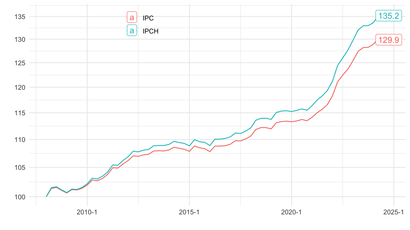
2017T2-2024T2
Code
`IPCH-IPC-2015-ensemble-Q` %>%
  filter(date >= zoo::as.yearqtr("2017 Q2"),
         date <= zoo::as.yearqtr("2024 Q2")) %>%
  arrange(date) %>%
  group_by(INDICATEUR) %>%
  mutate(OBS_VALUE = 100*OBS_VALUE/OBS_VALUE[1]) %>%
  ggplot + geom_line(aes(x = date, y = OBS_VALUE, color = INDICATEUR)) +
  xlab("") + ylab("") + theme_minimal() +
  theme(legend.title = element_blank(),
        legend.position = c(0.3, 0.9),
        axis.text.x = element_text(angle = 45, vjust = 1, hjust = 1)) +
  scale_x_yearqtr(labels = date_format("%YT%q"),
                  breaks = expand.grid(seq(1999, 2100, 1), c(1, 3)) %>%
                         mutate(breaks = zoo::as.yearqtr(paste0(Var1, "Q", Var2))) %>%
                         pull(breaks)) +
  scale_y_log10(breaks = seq(0, 1000, 5)) +
  geom_label(data = . %>% filter(date == max(date)),
             aes(x = date, y = OBS_VALUE, color = INDICATEUR, label = round(OBS_VALUE, 1)),
             show.legend = F)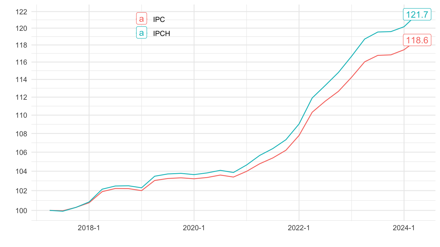
2017T1-
Code
`IPCH-IPC-2015-ensemble-Q` %>%
  filter(date >= zoo::as.yearqtr("2017 Q1")) %>%
  arrange(date) %>%
  group_by(INDICATEUR) %>%
  mutate(OBS_VALUE = 100*OBS_VALUE/OBS_VALUE[1]) %>%
  ggplot + geom_line(aes(x = date, y = OBS_VALUE, color = INDICATEUR)) +
  xlab("") + ylab("") + theme_minimal() +
  theme(legend.title = element_blank(),
        legend.position = c(0.3, 0.9),
        axis.text.x = element_text(angle = 45, vjust = 1, hjust = 1)) +
  scale_x_yearqtr(labels = date_format("%YT%q"),
                  breaks = expand.grid(seq(1999, 2100, 1), c(1, 3)) %>%
                         mutate(breaks = zoo::as.yearqtr(paste0(Var1, "Q", Var2))) %>%
                         pull(breaks)) +
  scale_y_log10(breaks = seq(0, 1000, 5)) +
  geom_label(data = . %>% filter(date == max(date)),
             aes(x = date, y = OBS_VALUE, color = INDICATEUR, label = round(OBS_VALUE, 1)),
             show.legend = F)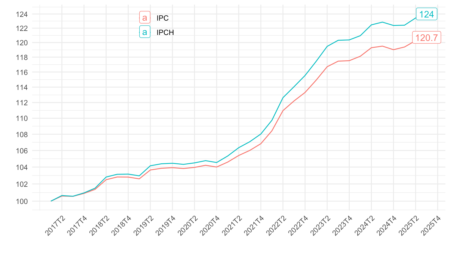
2017T2-
Code
`IPCH-IPC-2015-ensemble-Q` %>%
  filter(date >= zoo::as.yearqtr("2017 Q2")) %>%
  arrange(date) %>%
  group_by(INDICATEUR) %>%
  mutate(OBS_VALUE = 100*OBS_VALUE/OBS_VALUE[1]) %>%
  ggplot + geom_line(aes(x = date, y = OBS_VALUE, color = INDICATEUR)) +
  xlab("") + ylab("") + theme_minimal() +
  theme(legend.title = element_blank(),
        legend.position = c(0.3, 0.9),
        axis.text.x = element_text(angle = 45, vjust = 1, hjust = 1)) +
  scale_x_yearqtr(labels = date_format("%YT%q"),
                  breaks = expand.grid(seq(1999, 2100, 1), c(1, 3)) %>%
                         mutate(breaks = zoo::as.yearqtr(paste0(Var1, "Q", Var2))) %>%
                         pull(breaks)) +
  scale_y_log10(breaks = seq(0, 1000, 5)) +
  geom_label(data = . %>% filter(date == max(date)),
             aes(x = date, y = OBS_VALUE, color = INDICATEUR, label = round(OBS_VALUE, 1)),
             show.legend = F)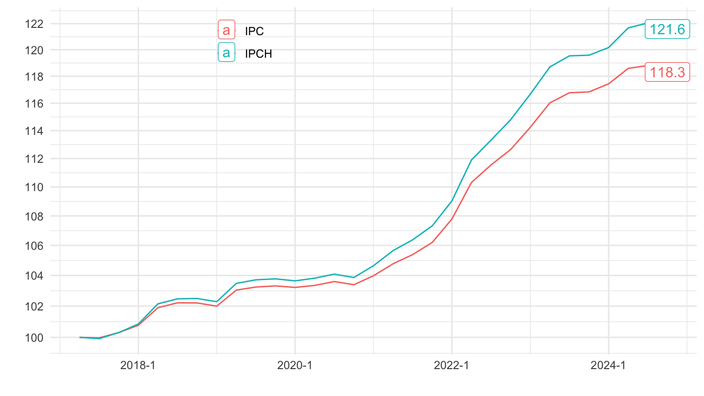
2021T4-
Code
`IPCH-IPC-2015-ensemble-Q` %>%
  filter(date >= zoo::as.yearqtr("2021 Q4")) %>%
  arrange(date) %>%
  group_by(INDICATEUR) %>%
  mutate(OBS_VALUE = 100*OBS_VALUE/OBS_VALUE[1]) %>%
  ggplot + geom_line(aes(x = date, y = OBS_VALUE, color = INDICATEUR)) +
  xlab("") + ylab("") + theme_minimal() +
  theme(legend.title = element_blank(),
        legend.position = c(0.3, 0.9),
        axis.text.x = element_text(angle = 45, vjust = 1, hjust = 1)) +
  scale_x_yearqtr(labels = date_format("%YT%q"),
                  breaks = expand.grid(seq(1999, 2100, 1), 1:4) %>%
                         mutate(breaks = zoo::as.yearqtr(paste0(Var1, "Q", Var2))) %>%
                         pull(breaks)) +
  scale_y_log10(breaks = seq(0, 1000, 5)) +
  geom_label(data = . %>% filter(date == max(date)),
             aes(x = date, y = OBS_VALUE, color = INDICATEUR, label = round(OBS_VALUE, 1)),
             show.legend = F)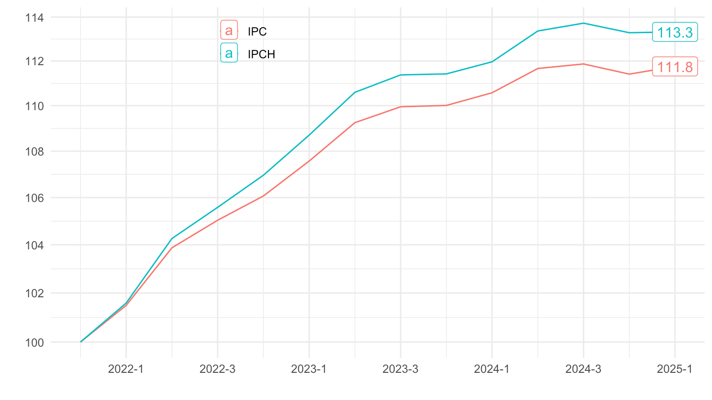
Mensuel
2008-
Code
`IPCH-IPC-2015-ensemble` %>%
  month_to_date %>%
  filter(date >= as.Date("2008-01-01")) %>%
  group_by(Indicateur) %>%
  arrange(date) %>%
  mutate(OBS_VALUE = 100*OBS_VALUE/OBS_VALUE[1]) %>%
  ggplot() + ylab("Indice des prix, Ensemble") + xlab("") + theme_minimal() +
  geom_line(aes(x = date, y = OBS_VALUE, color = Indicateur)) +

  scale_x_date(breaks = seq(1920, 2100, 2) %>% paste0("-01-01") %>% as.Date,
               labels = date_format("%Y")) +
  theme(legend.position = c(0.3, 0.8),
        legend.title = element_blank()) +
  scale_y_log10(breaks = seq(10, 300, 2),
                     labels = dollar_format(accuracy = 1, prefix = "")) +
  geom_label(data = . %>%
               filter(date == max(date)), aes(date, y = OBS_VALUE, label = round(OBS_VALUE, 1), color = Indicateur),
             show.legend = F)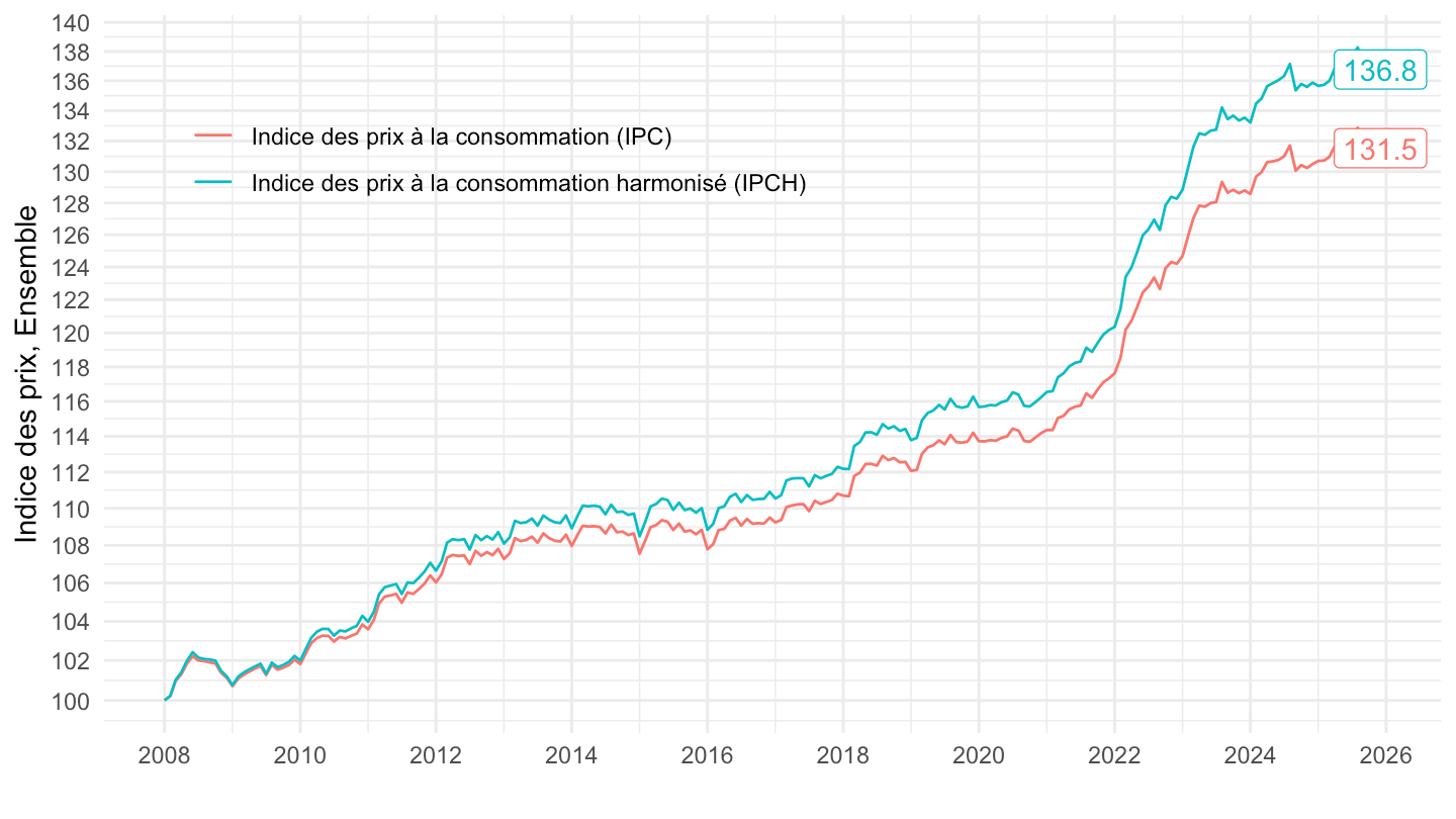
2017-
Code
`IPCH-IPC-2015-ensemble` %>%
  month_to_date %>%
  filter(date >= as.Date("2017-01-01")) %>%
  group_by(Indicateur) %>%
  arrange(date) %>%
  mutate(OBS_VALUE = 100*OBS_VALUE/OBS_VALUE[1]) %>%
  ggplot() + ylab("Indice des prix, Ensemble") + xlab("") + theme_minimal() +
  geom_line(aes(x = date, y = OBS_VALUE, color = Indicateur)) +

  scale_x_date(breaks = seq(1920, 2100, 1) %>% paste0("-01-01") %>% as.Date,
               labels = date_format("%Y")) +
  theme(legend.position = c(0.3, 0.8),
        legend.title = element_blank()) +
  scale_y_log10(breaks = seq(10, 300, 2),
                     labels = dollar_format(accuracy = 1, prefix = "")) +
  geom_label(data = . %>%
               filter(date == max(date)), aes(date, y = OBS_VALUE, label = round(OBS_VALUE, 1), color = Indicateur),
             show.legend = F)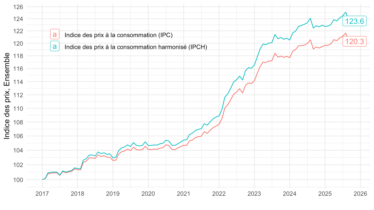
Ratio IPC IPCH
Annuel
1996-
Code
`IPCH-IPC-2015-ensemble-A` %>%
  filter(date >= zoo::as.Date("1996-01-01")) %>%
  arrange(date) %>%
  spread(INDICATEUR, OBS_VALUE) %>%
  mutate(OBS_VALUE = 100*IPCH/IPC) %>%
  mutate(OBS_VALUE = 100*OBS_VALUE/OBS_VALUE[1]) %>%
  ggplot + geom_line(aes(x = date, y = OBS_VALUE)) +
  xlab("") + ylab("") + theme_minimal() +
  theme(legend.title = element_blank(),
        legend.position = c(0.3, 0.9)) +
  scale_x_date(breaks = seq(1920, 2100, 2) %>% paste0("-01-01") %>% as.Date(),
               labels = date_format("%Y")) +
  scale_y_log10(breaks = seq(0, 1000, 1)) +
  geom_label_repel(data = . %>% filter(date == max(date)),
             aes(x = date, y = OBS_VALUE, label = round(OBS_VALUE, 1)))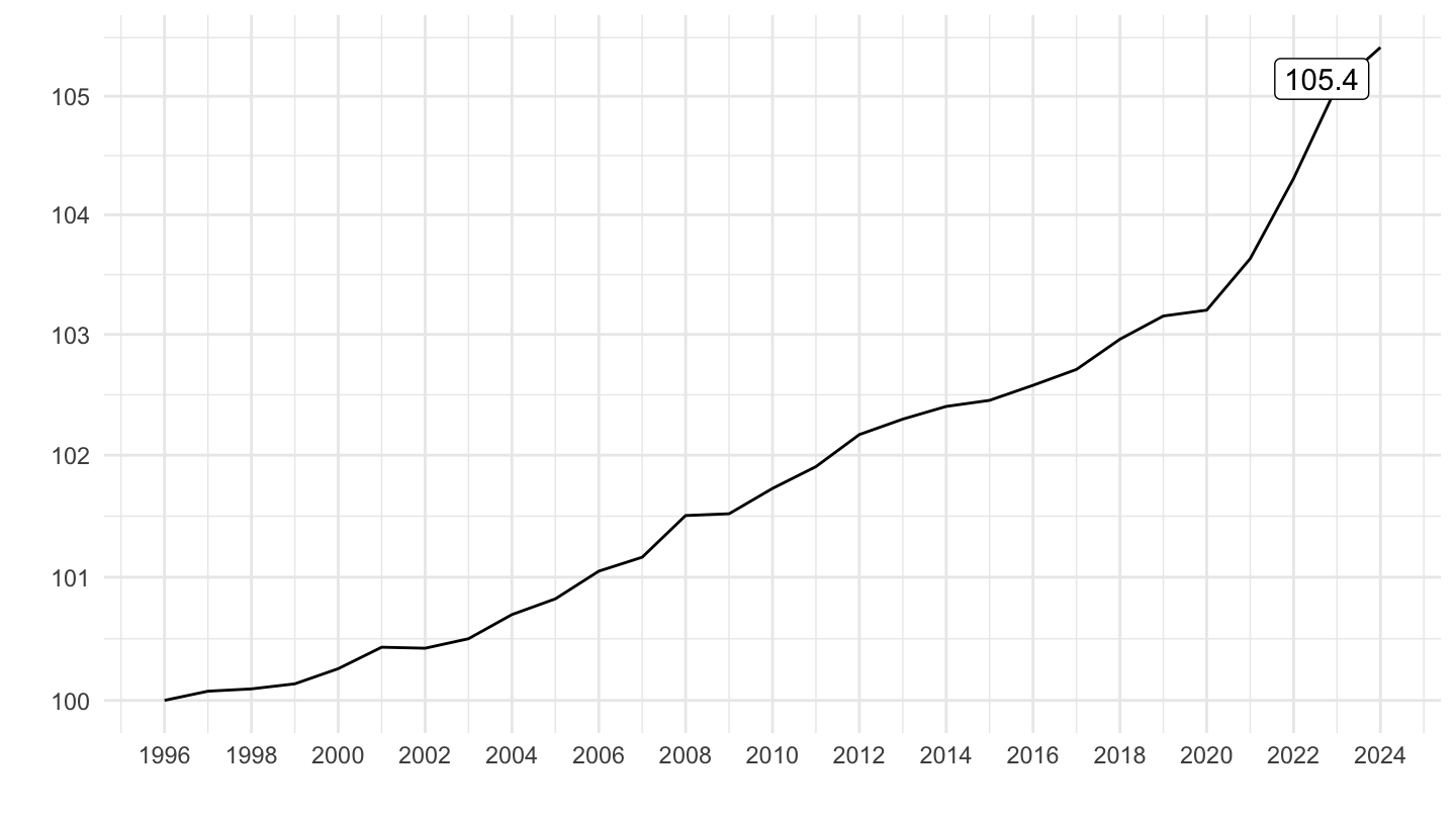
1999-
Code
`IPCH-IPC-2015-ensemble-A` %>%
  filter(date >= zoo::as.Date("1999-01-01")) %>%
  arrange(date) %>%
  spread(INDICATEUR, OBS_VALUE) %>%
  mutate(OBS_VALUE = 100*IPCH/IPC) %>%
  mutate(OBS_VALUE = 100*OBS_VALUE/OBS_VALUE[1]) %>%
  ggplot + geom_line(aes(x = date, y = OBS_VALUE)) +
  xlab("") + ylab("") + theme_minimal() +
  theme(legend.title = element_blank(),
        legend.position = c(0.3, 0.9)) +
  scale_x_date(breaks = seq(1920, 2100, 2) %>% paste0("-01-01") %>% as.Date(),
               labels = date_format("%Y")) +
  scale_y_log10(breaks = seq(0, 1000, 1)) +
  geom_label_repel(data = . %>% filter(date == max(date)),
             aes(x = date, y = OBS_VALUE, label = round(OBS_VALUE, 1)))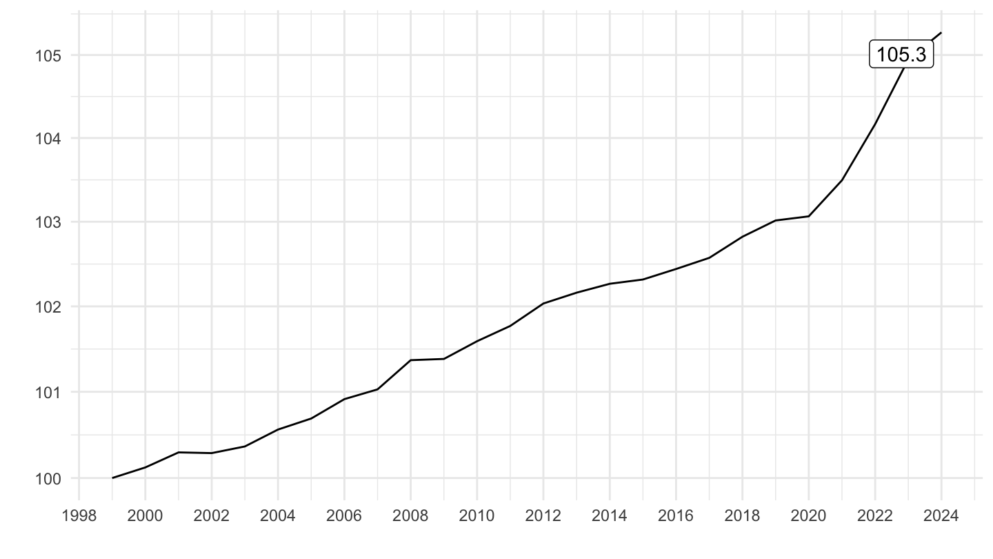
2008-
Code
`IPCH-IPC-2015-ensemble-A` %>%
  filter(date >= zoo::as.Date("2008-01-01")) %>%
  arrange(date) %>%
  spread(INDICATEUR, OBS_VALUE) %>%
  mutate(OBS_VALUE = 100*IPCH/IPC) %>%
  mutate(OBS_VALUE = 100*OBS_VALUE/OBS_VALUE[1]) %>%
  ggplot + geom_line(aes(x = date, y = OBS_VALUE)) +
  xlab("") + ylab("") + theme_minimal() +
  theme(legend.title = element_blank(),
        legend.position = c(0.3, 0.9)) +
  scale_x_date(breaks = seq(1920, 2100, 1) %>% paste0("-01-01") %>% as.Date(),
               labels = date_format("%Y")) +
  scale_y_log10(breaks = seq(0, 1000, 1)) +
  geom_label_repel(data = . %>% filter(date == max(date)),
             aes(x = date, y = OBS_VALUE, label = round(OBS_VALUE, 1)))
2008-2024
Code
`IPCH-IPC-2015-ensemble-A` %>%
  filter(date >= zoo::as.Date("2008-01-01"),
         date <= zoo::as.Date("2024-01-01")) %>%
  arrange(date) %>%
  spread(INDICATEUR, OBS_VALUE) %>%
  mutate(OBS_VALUE = 100*IPCH/IPC) %>%
  mutate(OBS_VALUE = 100*OBS_VALUE/OBS_VALUE[1]) %>%
  ggplot + geom_line(aes(x = date, y = OBS_VALUE)) +
  xlab("") + ylab("") + theme_minimal() +
  theme(legend.title = element_blank(),
        legend.position = c(0.3, 0.9)) +
  scale_x_date(breaks = seq(1920, 2100, 1) %>% paste0("-01-01") %>% as.Date(),
               labels = date_format("%Y")) +
  scale_y_log10(breaks = seq(0, 1000, 1)) +
  geom_label_repel(data = . %>% filter(date == max(date)),
             aes(x = date, y = OBS_VALUE, label = round(OBS_VALUE, 1)))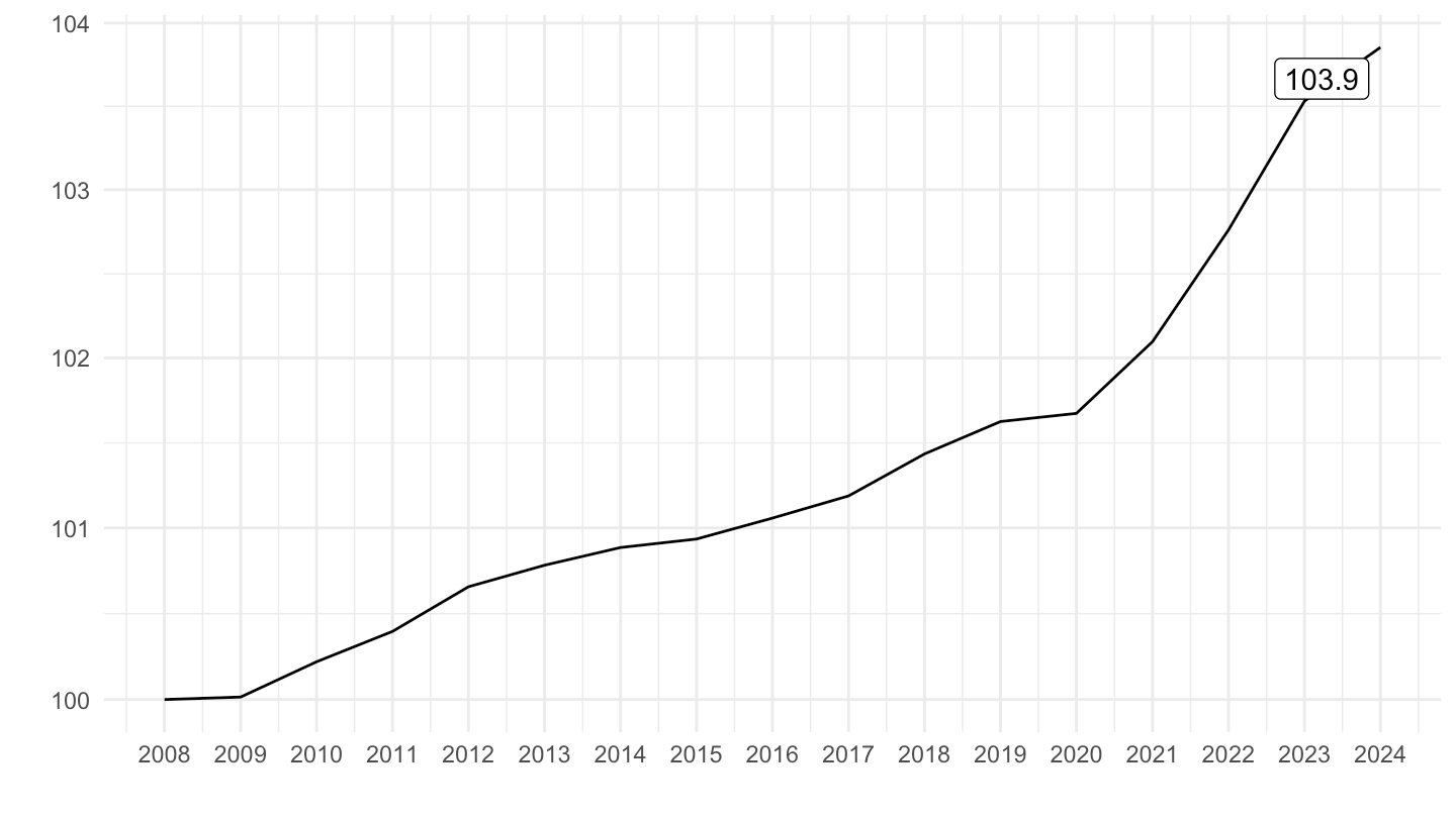
2017-
Code
`IPCH-IPC-2015-ensemble-A` %>%
  filter(date >= zoo::as.Date("2017-01-01")) %>%
  arrange(date) %>%
  spread(INDICATEUR, OBS_VALUE) %>%
  mutate(OBS_VALUE = 100*IPCH/IPC) %>%
  mutate(OBS_VALUE = 100*OBS_VALUE/OBS_VALUE[1]) %>%
  ggplot + geom_line(aes(x = date, y = OBS_VALUE)) +
  xlab("") + ylab("") + theme_minimal() +
  theme(legend.title = element_blank(),
        legend.position = c(0.3, 0.9)) +
  scale_x_date(breaks = seq(1920, 2100, 1) %>% paste0("-01-01") %>% as.Date(),
               labels = date_format("%Y")) +
  scale_y_log10(breaks = seq(0, 1000, 1)) +
  geom_label_repel(data = . %>% filter(date == max(date)),
             aes(x = date, y = OBS_VALUE, label = round(OBS_VALUE, 1)))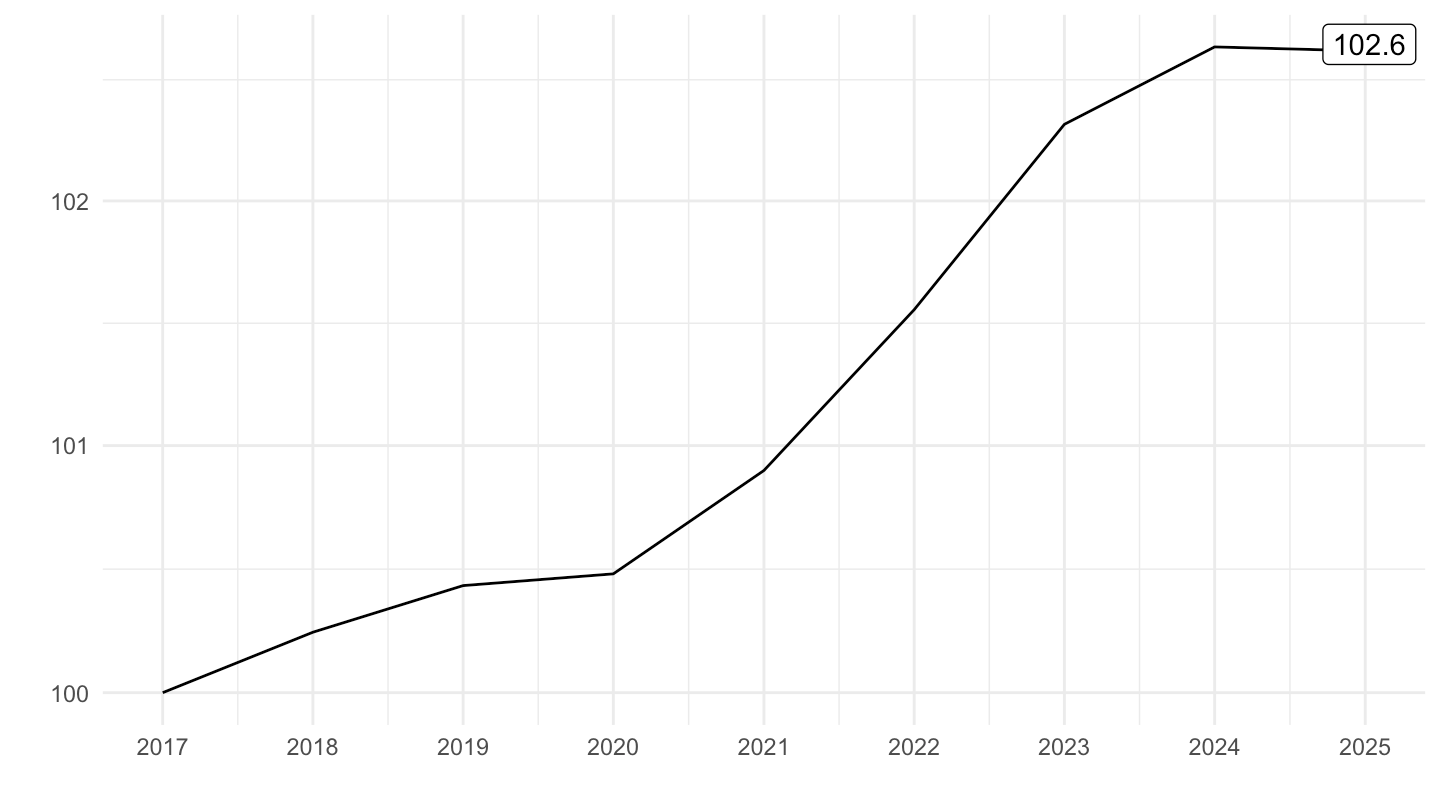
2019-2024
Code
`IPCH-IPC-2015-ensemble-A` %>%
  filter(date >= zoo::as.Date("2019-01-01"),
         date <= zoo::as.Date("2024-01-01")) %>%
  arrange(date) %>%
  spread(INDICATEUR, OBS_VALUE) %>%
  mutate(OBS_VALUE = 100*IPCH/IPC) %>%
  mutate(OBS_VALUE = 100*OBS_VALUE/OBS_VALUE[1]) %>%
  ggplot + geom_line(aes(x = date, y = OBS_VALUE)) +
  xlab("") + ylab("") + theme_minimal() +
  theme(legend.title = element_blank(),
        legend.position = c(0.3, 0.9)) +
  scale_x_date(breaks = seq(1920, 2100, 1) %>% paste0("-01-01") %>% as.Date(),
               labels = date_format("%Y")) +
  scale_y_log10(breaks = seq(0, 1000, 1)) +
  geom_label_repel(data = . %>% filter(date == max(date)),
             aes(x = date, y = OBS_VALUE, label = round(OBS_VALUE, 1)))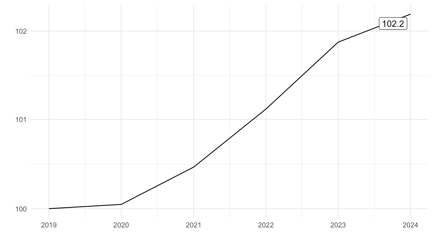
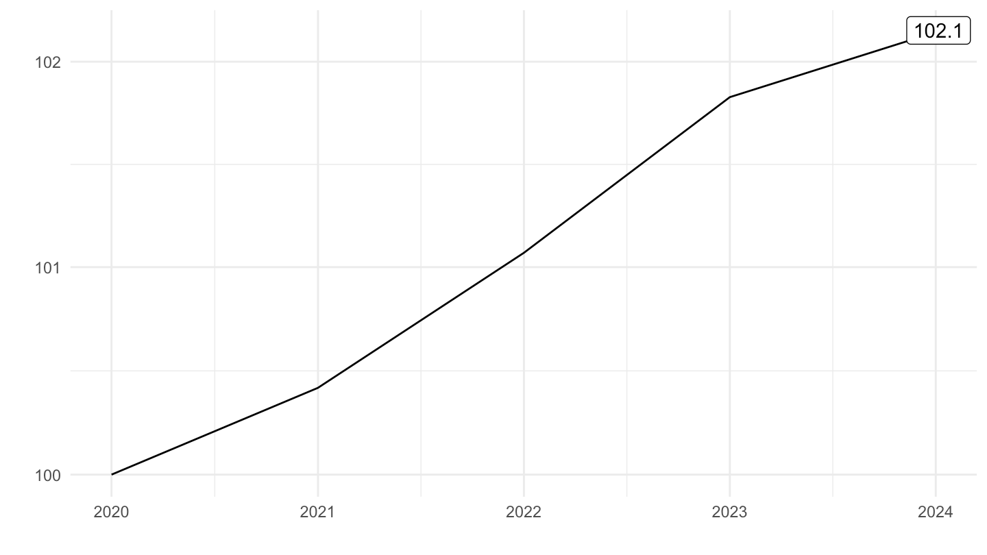
2020-
Code
`IPCH-IPC-2015-ensemble-A` %>%
  filter(date >= zoo::as.Date("2020-01-01")) %>%
  arrange(date) %>%
  spread(INDICATEUR, OBS_VALUE) %>%
  mutate(OBS_VALUE = 100*IPCH/IPC) %>%
  mutate(OBS_VALUE = 100*OBS_VALUE/OBS_VALUE[1]) %>%
  ggplot + geom_line(aes(x = date, y = OBS_VALUE)) +
  xlab("") + ylab("") + theme_minimal() +
  theme(legend.title = element_blank(),
        legend.position = c(0.3, 0.9)) +
  scale_x_date(breaks = seq(1920, 2100, 1) %>% paste0("-01-01") %>% as.Date(),
               labels = date_format("%Y")) +
  scale_y_log10(breaks = seq(0, 1000, 1)) +
  geom_label_repel(data = . %>% filter(date == max(date)),
             aes(x = date, y = OBS_VALUE, label = round(OBS_VALUE, 1)))