Prix moyens de vente de détail
Données - INSEE
Info
Last observation: 2026-06
First observation: 1992
Number of observations: 43 472
Last data update: 23 jul 2026, 22:50. Last compile: 24 jul 2026, 06:06
Structure
Données sur l’inflation en France
| source | dataset | Title | .html | .rData |
|---|---|---|---|---|
| insee | ILC-ILAT-ICC | Indices pour la révision d’un bail commercial ou professionnel | 2026-07-23 | 2026-07-23 |
| insee | INDICES_LOYERS | Indices des loyers d'habitation (ILH) | 2026-07-23 | 2026-07-23 |
| insee | IPC-1970-1980 | Indice des prix à la consommation - Base 1970, 1980 | 2026-07-23 | 2026-07-23 |
| insee | IPC-1990 | Indices des prix à la consommation - Base 1990 | 2026-07-23 | 2026-07-23 |
| insee | IPC-2015 | Indice des prix à la consommation - Base 2015 | 2026-07-23 | 2026-07-23 |
| insee | IPC-PM-2015 | Prix moyens de vente de détail | 2026-07-23 | 2026-07-23 |
| insee | IPCH-2015 | Indices des prix à la consommation harmonisés | 2026-07-23 | 2026-07-23 |
| insee | IPCH-IPC-2015-ensemble | Indices des prix à la consommation harmonisés | 2026-07-23 | 2026-07-23 |
| insee | IPGD-2015 | Indice des prix dans la grande distribution | 2026-07-23 | 2026-07-23 |
| insee | IPLA-IPLNA-2015 | Indices des prix des logements neufs et Indices Notaires-Insee des prix des logements anciens | 2026-07-23 | 2026-07-23 |
| insee | IPPI-2015 | Indices de prix de production et d'importation dans l'industrie | 2026-07-23 | 2026-07-23 |
| insee | IRL | Indice pour la révision d’un loyer d’habitation | 2026-07-23 | 2026-07-23 |
| insee | SERIES_LOYERS | Variation des loyers | 2026-07-23 | 2026-07-23 |
| insee | T_CONSO_EFF_FONCTION | Consommation effective des ménages par fonction | 2026-07-23 | 2025-12-22 |
| insee | bdf2017 | Budget de famille 2017 | 2026-07-23 | 2023-11-21 |
| insee | echantillon-agglomerations-IPC-2024 | Échantillon d’agglomérations enquêtées de l’IPC en 2024 | 2026-07-23 | 2026-01-27 |
| insee | echantillon-agglomerations-IPC-2025 | Échantillon d’agglomérations enquêtées de l’IPC en 2025 | 2026-07-23 | 2026-01-27 |
| insee | liste-varietes-IPC-2024 | Liste des variétés pour la mesure de l'IPC en 2024 | 2026-07-23 | 2025-04-02 |
| insee | liste-varietes-IPC-2025 | Liste des variétés pour la mesure de l'IPC en 2025 | 2026-07-23 | 2026-01-27 |
| insee | ponderations-elementaires-IPC-2024 | Pondérations élémentaires 2024 intervenant dans le calcul de l’IPC | 2026-07-23 | 2025-04-02 |
| insee | ponderations-elementaires-IPC-2025 | Pondérations élémentaires 2025 intervenant dans le calcul de l’IPC | 2026-07-23 | 2026-01-27 |
| insee | table_conso_moyenne_par_categorie_menages | Montants de consommation selon différentes catégories de ménages | 2026-07-23 | 2026-01-27 |
| insee | table_poste_au_sein_sous_classe_ecoicopv2_france_entiere_ | Ventilation de chaque sous-classe (niveau 4 de la COICOP v2) en postes et leurs pondérations | 2026-07-23 | 2026-01-27 |
| insee | tranches_unitesurbaines | Poids de chaque tranche d’unités urbaines dans la consommation | 2026-07-23 | 2026-01-27 |
Data on inflation
| source | dataset | Title | .html | .rData |
|---|---|---|---|---|
| bis | CPI | Consumer Price Index | 2026-07-22 | 2026-07-22 |
| ecb | CES | Consumer Expectations Survey | 2026-07-23 | 2026-07-19 |
| eurostat | nama_10_co3_p3 | Final consumption expenditure of households by consumption purpose (COICOP 3 digit) | 2026-07-18 | 2026-07-23 |
| eurostat | prc_hicp_cow | HICP - country weights | 2026-07-23 | 2026-07-23 |
| eurostat | prc_hicp_ctrb | Contributions to euro area annual inflation (in percentage points) | 2026-07-23 | 2026-07-23 |
| eurostat | prc_hicp_inw | HICP - item weights | 2026-07-23 | 2026-07-23 |
| eurostat | prc_hicp_manr | HICP (2015 = 100) - monthly data (annual rate of change) | 2026-07-23 | 2026-07-23 |
| eurostat | prc_hicp_midx | HICP (2015 = 100) - monthly data (index) | 2026-07-23 | 2026-07-23 |
| eurostat | prc_hicp_mmor | HICP (2015 = 100) - monthly data (monthly rate of change) | 2026-07-23 | 2026-07-23 |
| eurostat | prc_ppp_ind | Purchasing power parities (PPPs), price level indices and real expenditures for ESA 2010 aggregates | 2026-07-22 | 2026-07-23 |
| eurostat | sts_inpp_m | Producer prices in industry, total - monthly data | 2026-07-21 | 2026-07-23 |
| eurostat | sts_inppd_m | Producer prices in industry, domestic market - monthly data | 2026-07-21 | 2026-07-23 |
| eurostat | sts_inppnd_m | Producer prices in industry, non domestic market - monthly data | 2026-07-21 | 2026-07-23 |
| fred | cpi | Consumer Price Index | 2026-07-22 | 2026-07-22 |
| fred | inflation | Inflation | 2026-07-22 | 2026-07-22 |
| imf | CPI | Consumer Price Index (CPI) 2026 February - CPI_2026_FEB_VINTAGE | 2026-07-22 | 2026-04-13 |
| oecd | MEI_PRICES_PPI | Producer Prices - MEI_PRICES_PPI | 2026-07-23 | 2024-04-15 |
| oecd | PPP2017 | 2017 PPP Benchmark results | 2024-04-16 | 2023-07-25 |
| oecd | PRICES_CPI | Consumer price indices (CPIs) | 2024-04-16 | 2024-04-15 |
| wdi | FP.CPI.TOTL.ZG | Inflation, consumer prices (annual %) | 2026-07-22 | 2026-07-22 |
| wdi | NY.GDP.DEFL.KD.ZG | Inflation, GDP deflator (annual %) | 2026-07-22 | 2026-07-22 |
LAST_COMPILE
| LAST_COMPILE |
|---|
| 2026-07-24 |
Last
Code
`IPC-PM-2015` %>%
  group_by(TIME_PERIOD) %>%
  summarise(Nobs = n()) %>%
  arrange(desc(TIME_PERIOD)) %>%
  head(1) %>%
print_table_conditional()| TIME_PERIOD | Nobs |
|---|---|
| 2026-06 | 62 |
Prix Baguette
Tous
Indice
Code
`IPC-PM-2015` %>%
  filter(PRIX_CONSO %in% c("1223", "1227"),
         FREQ == "M") %>%

  month_to_date() %>%
  ggplot + theme_minimal() + xlab("") + ylab("Prix en €") +
  geom_line(aes(x = date, y = OBS_VALUE/4, color = Prix_conso)) +
  scale_x_date(breaks = seq(1960, 2100, 2) %>% paste0("-01-01") %>% as.Date,
               labels = date_format("%Y")) +
  scale_y_log10(breaks = seq(0, 3, 0.1),
                     labels = dollar_format(accuracy = .1, prefix = "", su = " €")) +

  theme(legend.position = c(0.7, 0.15),
        legend.title = element_blank())
Glissement Annuel
Code
`IPC-PM-2015` %>%
  filter(PRIX_CONSO %in% c("1223", "1227"),
         FREQ == "M") %>%

  month_to_date() %>%
  group_by(Prix_conso) %>%
  arrange(date) %>%
  mutate(inflation = OBS_VALUE/lag(OBS_VALUE,12)-1) %>%
  ggplot + theme_minimal() + xlab("") + ylab("Glissement annuel") +
  geom_line(aes(x = date, y = inflation, color = Prix_conso)) +
  scale_x_date(breaks = seq(1960, 2100, 2) %>% paste0("-01-01") %>% as.Date,
               labels = date_format("%Y")) +
  scale_y_continuous(breaks = 0.01*seq(-10, 30, 1),
                     labels = percent_format(acc = 1)) +
  theme(legend.position = c(0.3, 0.9),
        legend.title = element_blank())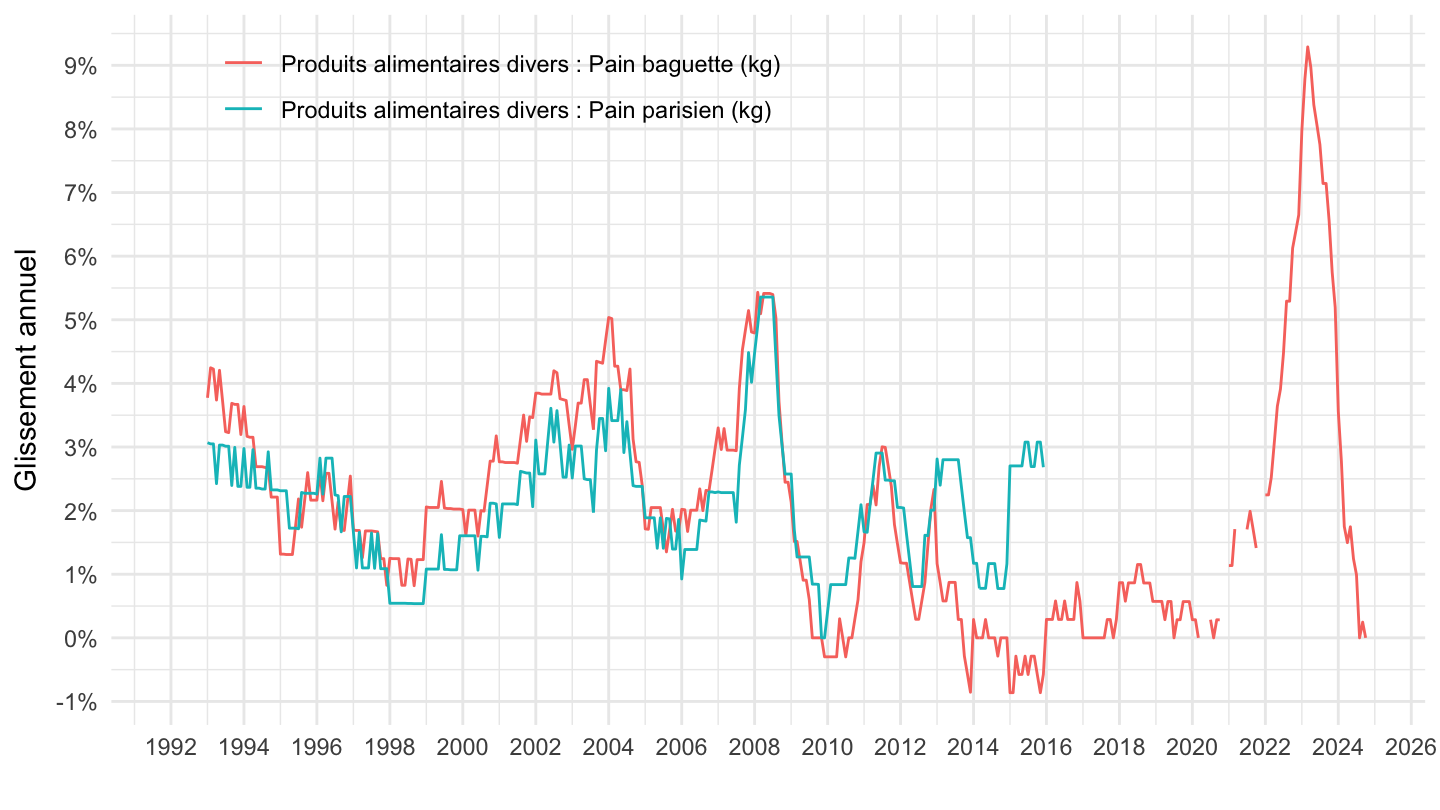
Immobilier, Pain Baguette
Code
t_5203_extract <- t_5203 %>%
  year_to_date2 %>%
  filter(sector %in% c("A10.LZ", "TOTAL")) %>%
  filter(date >= as.Date("1992-01-01")) %>%
  group_by(sector) %>%
  mutate(value = 100*value/value[date == as.Date("1992-01-01")]) %>%
  select(date, Variable = Sector, value)


data_extract <- `IPC-PM-2015` %>%
  filter(PRIX_CONSO %in% c("1223"),
         FREQ == "M") %>%
  left_join(PRIX_CONSO,  by = "PRIX_CONSO") %>%
  month_to_date() %>%
  mutate(Variable = "Prix de la baguette") %>%
  select(date, Variable, value = OBS_VALUE) %>%
  mutate(value = 100*value/value[date == as.Date("1992-01-01")])


croissant <- `IPC-PM-2015` %>%
  filter(PRIX_CONSO %in% c("1241"),
         FREQ == "M") %>%
  left_join(PRIX_CONSO,  by = "PRIX_CONSO") %>%
  month_to_date() %>%
  mutate(Variable = "Prix du croissant") %>%
  select(date, Variable, value = OBS_VALUE) %>%
  mutate(value = 100*value/value[date == as.Date("1992-01-01")])

t_5203_extract %>%
  bind_rows(data_extract) %>%
  bind_rows(croissant) %>%
  ggplot(.) + theme_minimal() + ylab("") + xlab("") +
  geom_line(aes(x = date, y = value, color = Variable)) +
  theme(legend.title = element_blank(),
        legend.position = c(0.2, 0.8)) +
  scale_x_date(breaks = seq(1950, 2022, 2) %>% paste0("-01-01") %>% as.Date,
               labels = date_format("%Y")) +

  scale_y_log10(breaks = seq(0, 200, 10))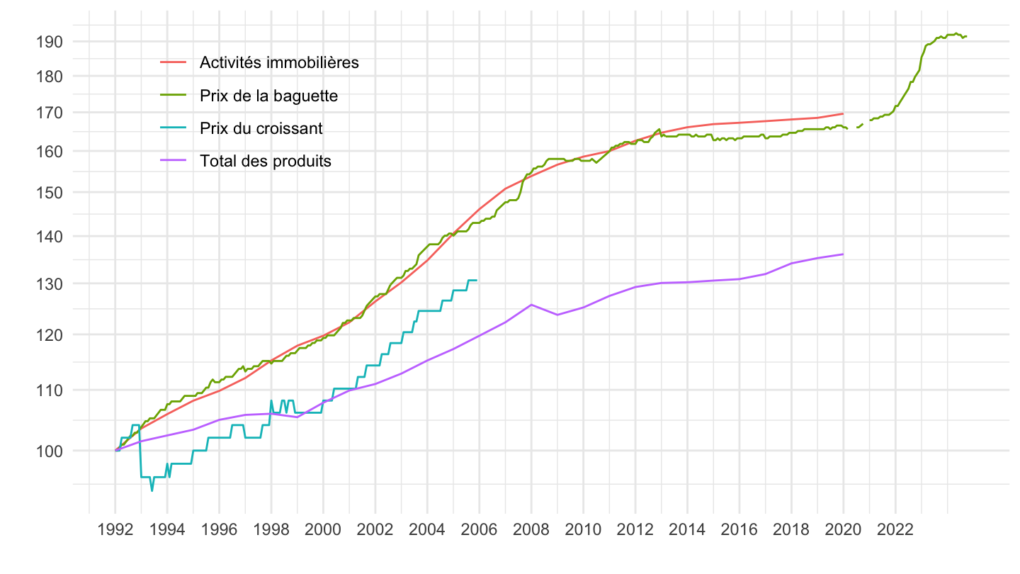
Gaz butane comprimé
Valeur
Code
`IPC-PM-2015` %>%
  filter(PRIX_CONSO %in% c("1873"),
         FREQ == "M") %>%
  mutate(OBS_VALUE = ifelse(PRIX_CONSO == "3790", OBS_VALUE/1000, OBS_VALUE)) %>%

  month_to_date() %>%
  mutate(Prix_conso = gsub("Non alimentaire : ", "", Prix_conso)) %>%
  mutate(Prix_conso = gsub(": 1.000 litres \\(livré à domicile\\)",
                           "\\(1 litre, livré à domicile\\)", Prix_conso)) %>%
  ggplot + theme_minimal() + xlab("") + ylab("Gaz butane comprimé") +
  geom_line(aes(x = date, y = OBS_VALUE, color = Prix_conso)) +
  scale_x_date(breaks = seq(1992, 2022, 5) %>% paste0("-01-01") %>% as.Date,
               labels = date_format("%Y")) +
  scale_y_continuous(breaks = seq(0, 40, 2),
                     labels = dollar_format(accuracy = 1, prefix = "", su = " €")) +

  theme(legend.position = c(0.3, 0.9),
        legend.title = element_blank())
Base 100
Code
`IPC-PM-2015` %>%
  filter(PRIX_CONSO %in% c("1873", "3863", "3860"),
         FREQ == "M") %>%
  mutate(OBS_VALUE = ifelse(PRIX_CONSO == "3790", OBS_VALUE/1000, OBS_VALUE)) %>%

  month_to_date() %>%
  mutate(Prix_conso = gsub("Non alimentaire : ", "", Prix_conso)) %>%
  mutate(Prix_conso = gsub(": 1.000 litres \\(livré à domicile\\)",
                           "\\(1 litre, livré à domicile\\)", Prix_conso)) %>%
  group_by(PRIX_CONSO) %>%
  arrange(date) %>%
  mutate(OBS_VALUE = 100*OBS_VALUE/OBS_VALUE[1]) %>%
  ggplot + theme_minimal() + xlab("") + ylab("") +
  geom_line(aes(x = date, y = OBS_VALUE, color = Prix_conso)) +
  scale_x_date(breaks = seq(1992, 2022, 5) %>% paste0("-01-01") %>% as.Date,
               labels = date_format("%Y")) +
  scale_y_log10(breaks = seq(100, 850, 20)) +

  theme(legend.position = c(0.3, 0.9),
        legend.title = element_blank())
Essence, Fioul, Gazole
Tous
Value - Linear
Code
`IPC-PM-2015` %>%
  filter(PRIX_CONSO %in% c("3860", "3790", "3863"),
         FREQ == "M") %>%
  mutate(OBS_VALUE = ifelse(PRIX_CONSO == "3790", OBS_VALUE/1000, OBS_VALUE)) %>%

  month_to_date() %>%
  mutate(Prix_conso = gsub("Non alimentaire : ", "", Prix_conso)) %>%
  mutate(Prix_conso = gsub(": 1.000 litres \\(livré à domicile\\)",
                           "\\(1 litre, livré à domicile\\)", Prix_conso)) %>%
  ggplot + theme_minimal() + xlab("") + ylab("1 litre en €") +
  geom_line(aes(x = date, y = OBS_VALUE, color = Prix_conso)) +
  scale_x_date(breaks = seq(1992, 2022, 5) %>% paste0("-01-01") %>% as.Date,
               labels = date_format("%Y")) +
  scale_y_continuous(breaks = seq(0, 3, 0.1),
                     labels = dollar_format(accuracy = .1, prefix = "", su = " €")) +

  theme(legend.position = c(0.3, 0.9),
        legend.title = element_blank())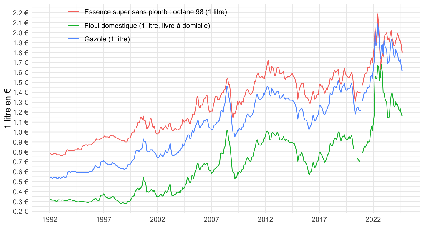
Value - Log
Code
`IPC-PM-2015` %>%
  filter(PRIX_CONSO %in% c("3860", "3790", "3863"),
         FREQ == "M") %>%
  mutate(OBS_VALUE = ifelse(PRIX_CONSO == "3790", OBS_VALUE/1000, OBS_VALUE)) %>%

  month_to_date() %>%
  mutate(Prix_conso = gsub("Non alimentaire : ", "", Prix_conso)) %>%
  mutate(Prix_conso = gsub(": 1.000 litres \\(livré à domicile\\)",
                           "\\(1 litre, livré à domicile\\)", Prix_conso)) %>%
  ggplot + theme_minimal() + xlab("") + ylab("1 litre en €") +
  geom_line(aes(x = date, y = OBS_VALUE, color = Prix_conso)) +
  scale_x_date(breaks = seq(1992, 2022, 5) %>% paste0("-01-01") %>% as.Date,
               labels = date_format("%Y")) +
  scale_y_log10(breaks = seq(0, 3, 0.1),
                     labels = dollar_format(accuracy = .1, prefix = "", su = " €")) +

  theme(legend.position = c(0.7, 0.2),
        legend.title = element_blank())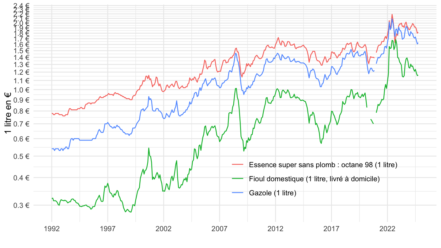
Indice
Code
`IPC-PM-2015` %>%
  filter(PRIX_CONSO %in% c("3860", "3790", "3863"),
         FREQ == "M") %>%
  mutate(OBS_VALUE = ifelse(PRIX_CONSO == "3790", OBS_VALUE/1000, OBS_VALUE)) %>%

  month_to_date() %>%
  mutate(Prix_conso = gsub("Non alimentaire : ", "", Prix_conso)) %>%
  mutate(Prix_conso = gsub(": 1.000 litres \\(livré à domicile\\)",
                           "\\(1 litre, livré à domicile\\)", Prix_conso)) %>%
  group_by(PRIX_CONSO) %>%
  arrange(date) %>%
  mutate(OBS_VALUE = 100*OBS_VALUE/OBS_VALUE[1]) %>%
  ggplot + theme_minimal() + xlab("") + ylab("") +
  geom_line(aes(x = date, y = OBS_VALUE, color = Prix_conso)) +
  scale_x_date(breaks = seq(1992, 2022, 5) %>% paste0("-01-01") %>% as.Date,
               labels = date_format("%Y")) +
  scale_y_log10(breaks = seq(100, 850, 50)) +

  theme(legend.position = c(0.7, 0.2),
        legend.title = element_blank())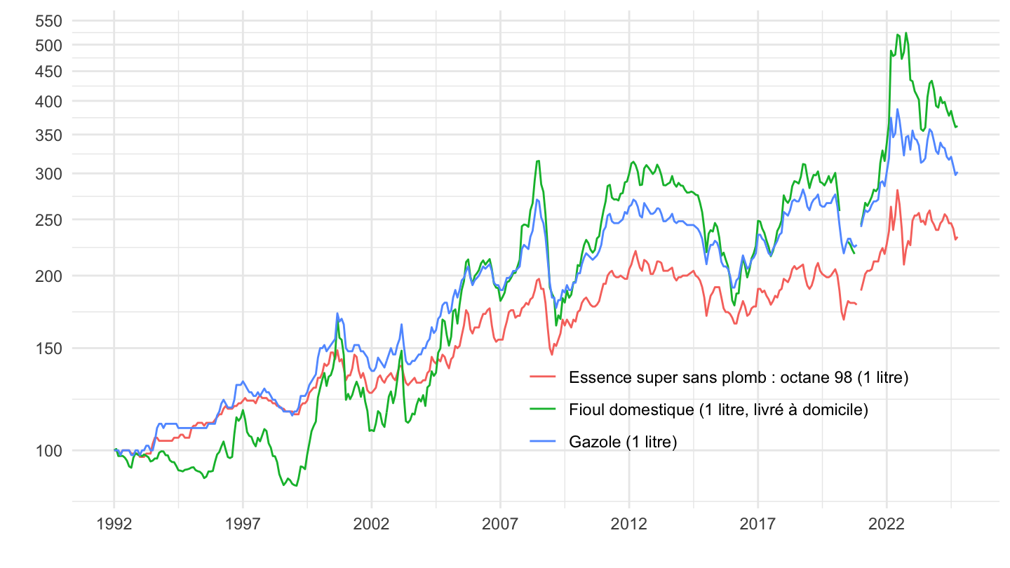
1996-
Value
Code
`IPC-PM-2015` %>%
  filter(PRIX_CONSO %in% c("3860", "3790", "3863"),
         FREQ == "M") %>%
  mutate(OBS_VALUE = ifelse(PRIX_CONSO == "3790", OBS_VALUE/1000, OBS_VALUE)) %>%

  month_to_date() %>%
  filter(date >= as.Date("1996-01-01")) %>%
  mutate(Prix_conso = gsub("Non alimentaire : ", "", Prix_conso)) %>%
  mutate(Prix_conso = gsub(": 1.000 litres \\(livré à domicile\\)",
                           "\\(1 litre, livré à domicile\\)", Prix_conso)) %>%
  ggplot + theme_minimal() + xlab("") + ylab("1 litre en €") +
  geom_line(aes(x = date, y = OBS_VALUE, color = Prix_conso)) +
  scale_x_date(breaks = seq(1960, 2100, 2) %>% paste0("-01-01") %>% as.Date,
               labels = date_format("%Y")) +
  scale_y_log10(breaks = seq(0, 3, 0.1),
                     labels = dollar_format(accuracy = .1, prefix = "", su = " €")) +

  theme(legend.position = c(0.7, 0.2),
        legend.title = element_blank())
Indice
Code
`IPC-PM-2015` %>%
  filter(PRIX_CONSO %in% c("3860", "3790", "3863"),
         FREQ == "M") %>%
  mutate(OBS_VALUE = ifelse(PRIX_CONSO == "3790", OBS_VALUE/1000, OBS_VALUE)) %>%

  month_to_date() %>%
  arrange(date) %>%
  filter(date >= as.Date("1996-01-01")) %>%
  group_by(PRIX_CONSO) %>%
  mutate(OBS_VALUE = 100*OBS_VALUE/OBS_VALUE[1]) %>%
  mutate(Prix_conso = gsub(": 1.000 litres \\(livré à domicile\\)",
                           "\\(1 litre, livré à domicile\\)", Prix_conso)) %>%
  ggplot + theme_minimal() + xlab("") + ylab("") +
  geom_line(aes(x = date, y = OBS_VALUE, color = Prix_conso)) +
  scale_x_date(breaks = seq(1960, 2100, 2) %>% paste0("-01-01") %>% as.Date,
               labels = date_format("%Y")) +
  scale_y_log10(breaks = seq(100, 850, 50)) +

  theme(legend.position = c(0.4, 0.9),
        legend.title = element_blank())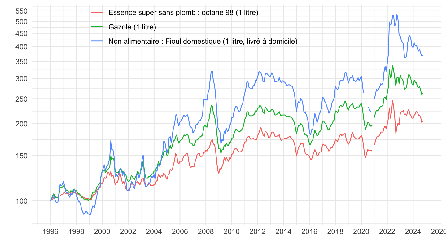
2015-
Value
Code
`IPC-PM-2015` %>%
  filter(PRIX_CONSO %in% c("3860", "3790", "3863"),
         FREQ == "M") %>%
  mutate(OBS_VALUE = ifelse(PRIX_CONSO == "3790", OBS_VALUE/1000, OBS_VALUE)) %>%

  month_to_date() %>%
  filter(date >= as.Date("2015-01-01")) %>%
  mutate(Prix_conso = gsub("Non alimentaire : ", "", Prix_conso)) %>%
  mutate(Prix_conso = gsub(": 1.000 litres \\(livré à domicile\\)",
                           "\\(1 litre, livré à domicile\\)", Prix_conso)) %>%
  ggplot + theme_minimal() + xlab("") + ylab("1 litre en €") +
  geom_line(aes(x = date, y = OBS_VALUE, color = Prix_conso)) +
  scale_x_date(breaks = seq(1960, 2100, 1) %>% paste0("-01-01") %>% as.Date,
               labels = date_format("%Y")) +
  scale_y_log10(breaks = seq(0, 3, 0.1),
                     labels = dollar_format(accuracy = .1, prefix = "", su = " €")) +
  theme(legend.position = c(0.3, 0.9),
        legend.title = element_blank())
Indice
Code
`IPC-PM-2015` %>%
  filter(PRIX_CONSO %in% c("3860", "3790", "3863"),
         FREQ == "M") %>%
  mutate(OBS_VALUE = ifelse(PRIX_CONSO == "3790", OBS_VALUE/1000, OBS_VALUE)) %>%

  month_to_date() %>%
  arrange(date) %>%
  filter(date >= as.Date("2015-01-01")) %>%
  group_by(PRIX_CONSO) %>%
  mutate(OBS_VALUE = 100*OBS_VALUE/OBS_VALUE[1]) %>%
  mutate(Prix_conso = gsub(": 1.000 litres \\(livré à domicile\\)",
                           "\\(1 litre, livré à domicile\\)", Prix_conso)) %>%
  ggplot + theme_minimal() + xlab("") + ylab("") +
  geom_line(aes(x = date, y = OBS_VALUE, color = Prix_conso)) +
  scale_x_date(breaks = seq(1960, 2100, 1) %>% paste0("-01-01") %>% as.Date,
               labels = date_format("%Y")) +
  scale_y_log10(breaks = seq(100, 850, 50)) +

  theme(legend.position = c(0.4, 0.9),
        legend.title = element_blank())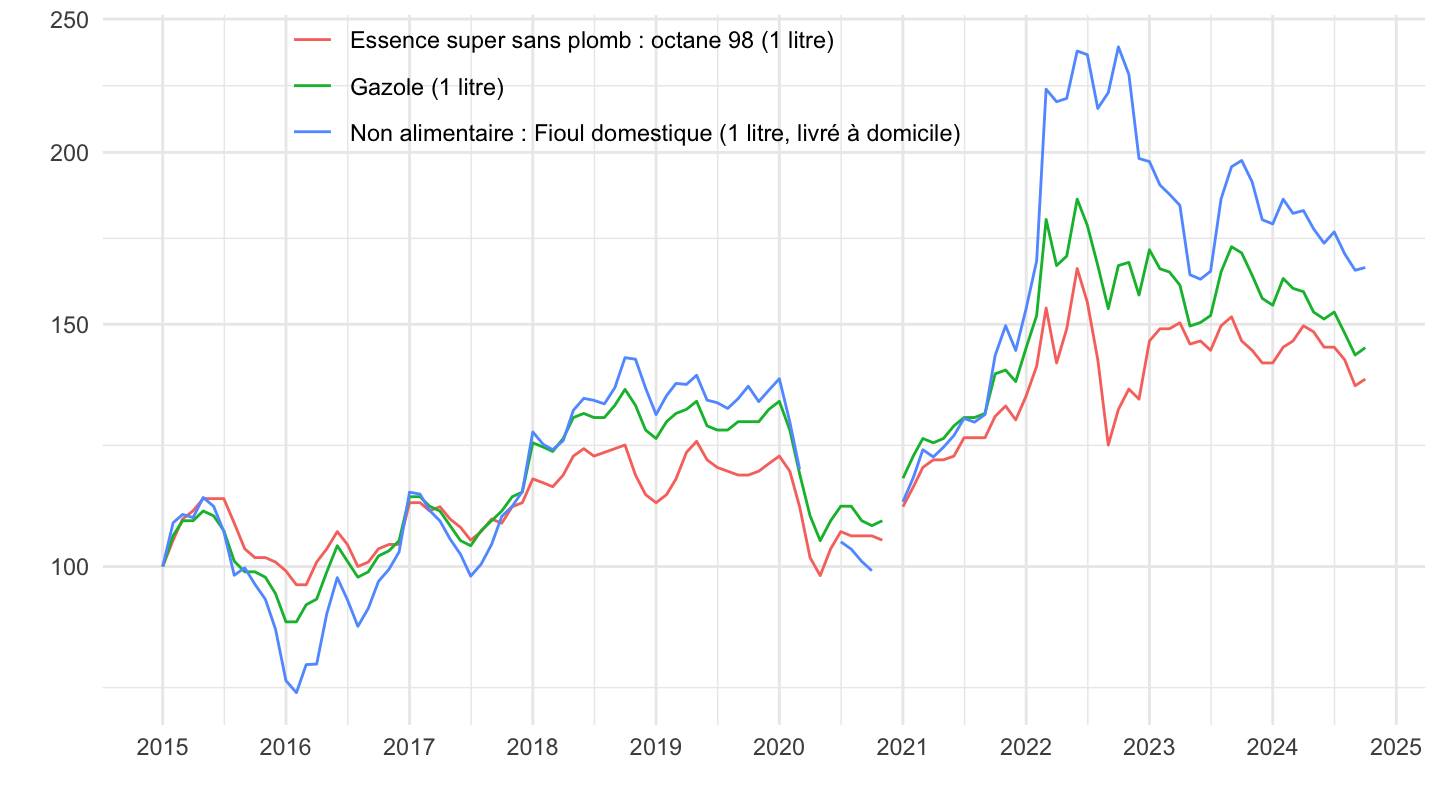
Essence, Gazole
Tous
Code
`IPC-PM-2015` %>%
  filter(PRIX_CONSO %in% c("3860", "3861", "3863"),
         FREQ == "M") %>%

  month_to_date() %>%
  ggplot + theme_minimal() + xlab("") + ylab("1 litre en €") +
  geom_line(aes(x = date, y = OBS_VALUE, color = Prix_conso)) +
  scale_x_date(breaks = seq(1960, 2100, 2) %>% paste0("-01-01") %>% as.Date,
               labels = date_format("%Y")) +
  scale_y_continuous(breaks = seq(0, 3, 0.1),
                     labels = dollar_format(accuracy = .1, prefix = "", su = " €")) +

  theme(legend.position = c(0.3, 0.9),
        legend.title = element_blank())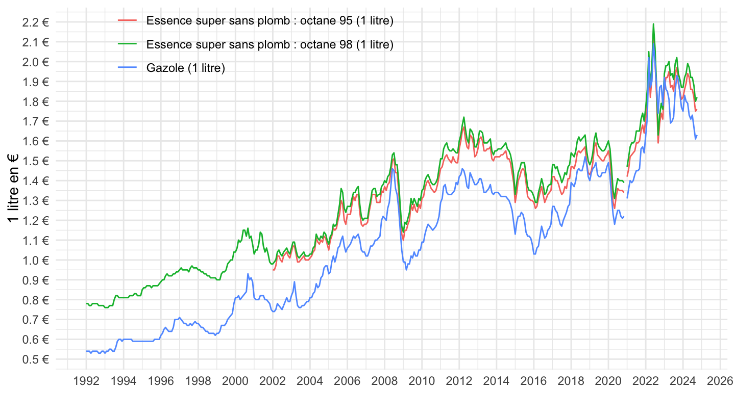
1996-
Value
Code
`IPC-PM-2015` %>%
  filter(PRIX_CONSO %in% c("3860", "3861", "3863"),
         FREQ == "M") %>%

  month_to_date() %>%
  filter(date >= as.Date("1996-01-01")) %>%
  ggplot + theme_minimal() + xlab("") + ylab("1 litre en €") +
  geom_line(aes(x = date, y = OBS_VALUE, color = Prix_conso)) +
  scale_x_date(breaks = seq(1960, 2100, 2) %>% paste0("-01-01") %>% as.Date,
               labels = date_format("%Y")) +
  scale_y_log10(breaks = seq(0, 3, 0.1),
                     labels = dollar_format(accuracy = .1, prefix = "", su = " €")) +

  theme(legend.position = c(0.25, 0.9),
        legend.title = element_blank())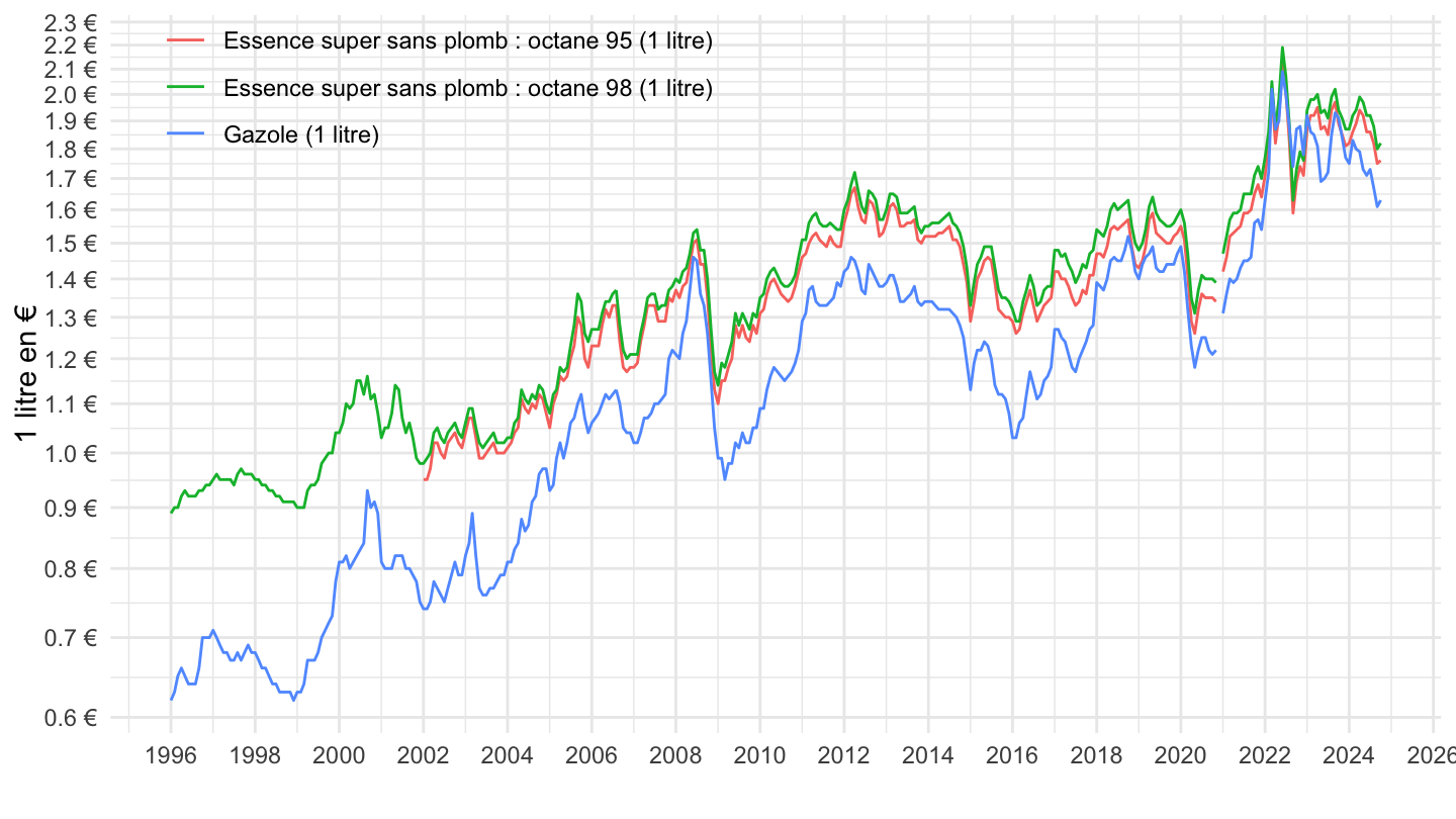
Indice
Code
`IPC-PM-2015` %>%
  filter(PRIX_CONSO %in% c("3860", "3863"),
         FREQ == "M") %>%

  month_to_date() %>%
  arrange(date) %>%
  filter(date >= as.Date("1996-01-01")) %>%
  group_by(PRIX_CONSO) %>%
  mutate(OBS_VALUE = 100*OBS_VALUE/OBS_VALUE[1]) %>%
  ggplot + theme_minimal() + xlab("") + ylab("") +
  geom_line(aes(x = date, y = OBS_VALUE, color = Prix_conso)) +
  scale_x_date(breaks = seq(1960, 2100, 2) %>% paste0("-01-01") %>% as.Date,
               labels = date_format("%Y")) +
  scale_y_log10(breaks = seq(100, 850, 10)) +

  theme(legend.position = c(0.25, 0.9),
        legend.title = element_blank())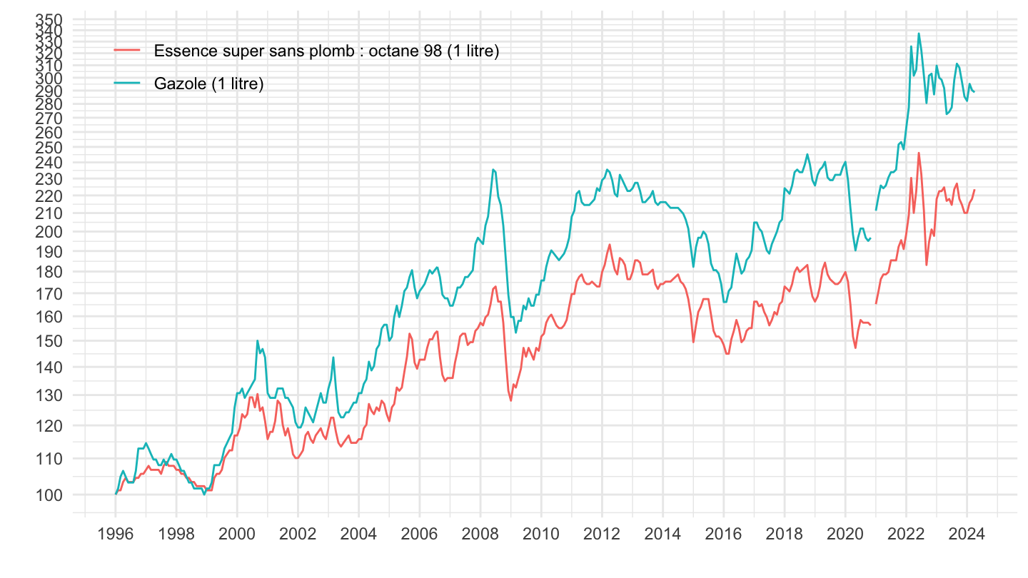
2002-
Code
`IPC-PM-2015` %>%
  filter(PRIX_CONSO %in% c("3860", "3861", "3863"),
         FREQ == "M") %>%

  month_to_date() %>%
  filter(date >= as.Date("2002-01-01")) %>%
  ggplot + theme_minimal() + xlab("") + ylab("1 litre en €") +
  geom_line(aes(x = date, y = OBS_VALUE, color = Prix_conso)) +
  scale_x_date(breaks = seq(1960, 2100, 2) %>% paste0("-01-01") %>% as.Date,
               labels = date_format("%Y")) +
  scale_y_continuous(breaks = seq(0, 3, 0.1),
                     labels = dollar_format(accuracy = .1, prefix = "", su = " €")) +

  theme(legend.position = c(0.25, 0.9),
        legend.title = element_blank())
2015-
Code
`IPC-PM-2015` %>%
  filter(PRIX_CONSO %in% c("3860", "3861", "3863"),
         FREQ == "M") %>%

  month_to_date() %>%
  filter(date >= as.Date("2015-01-01")) %>%
  arrange(desc(date)) %>%
  select(date, OBS_VALUE, Prix_conso, everything()) %>%
  ggplot + theme_minimal() + xlab("") + ylab("1 litre en €") +
  geom_line(aes(x = date, y = OBS_VALUE, color = Prix_conso)) +
  scale_x_date(breaks = seq(1960, 2100, 1) %>% paste0("-01-01") %>% as.Date,
               labels = date_format("%Y")) +
  scale_y_continuous(breaks = seq(0, 3, 0.1),
                     labels = dollar_format(accuracy = .1, prefix = "", su = " €")) +
  scale_color_manual(values = c("blue", "red", "black")) +
  theme(legend.position = c(0.25, 0.9),
        legend.title = element_blank())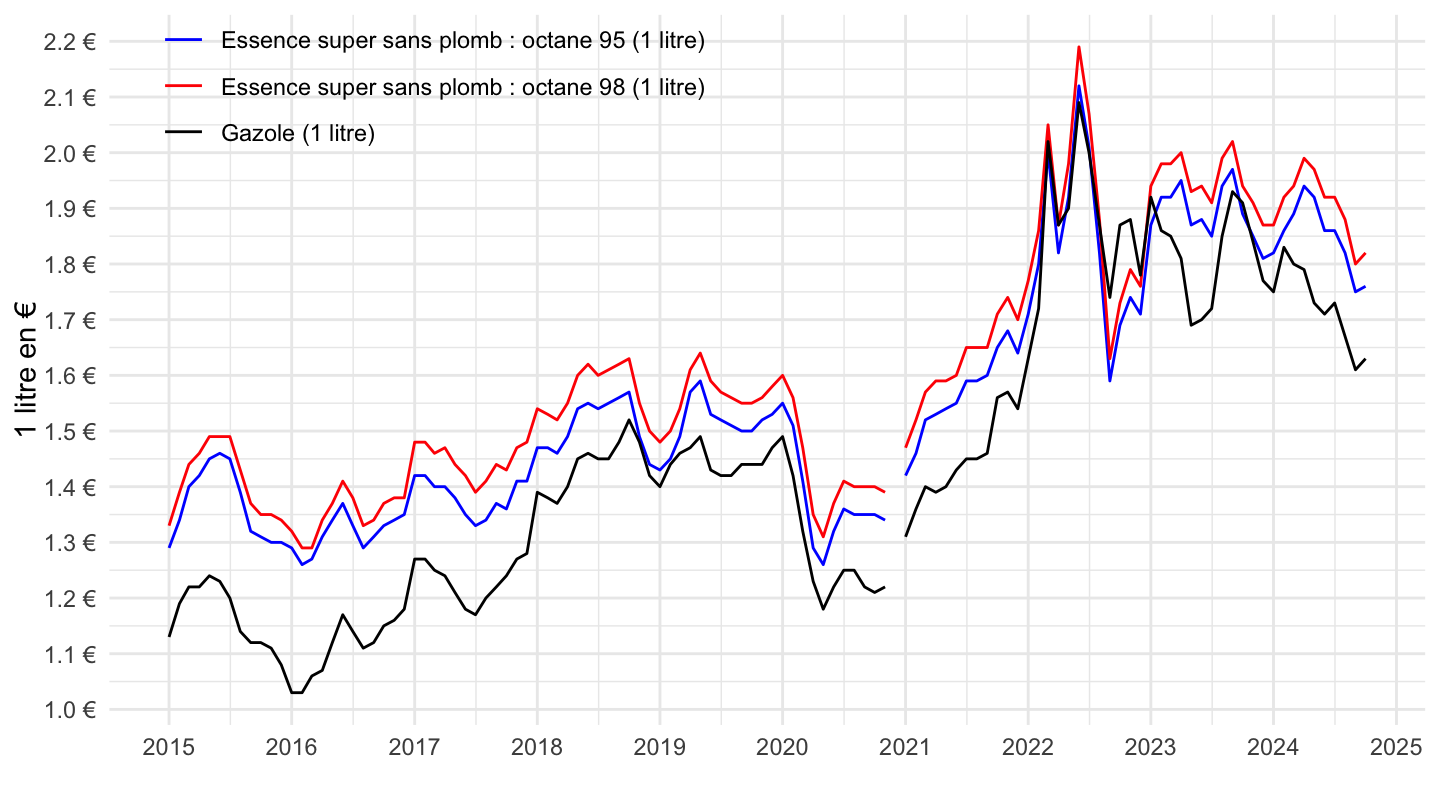
Viandes, Boissons
Entrecôte de boeuf, Porc, Veau, Poulet
1992-
Code
`IPC-PM-2015` %>%
  filter(PRIX_CONSO %in% c("1188", "1244", "1264", "1334"),
         FREQ == "M") %>%

  month_to_date() %>%
  ggplot + theme_minimal() + xlab("") + ylab("1 kg en €") +
  geom_line(aes(x = date, y = OBS_VALUE, color = Prix_conso)) +
  scale_x_date(breaks = seq(1960, 2100, 2) %>% paste0("-01-01") %>% as.Date,
               labels = date_format("%Y")) +
  scale_y_continuous(breaks = seq(0, 100, 1),
                     labels = dollar_format(accuracy = 1, prefix = "", su = " €")) +

  theme(legend.position = c(0.3, 0.9),
        legend.title = element_blank())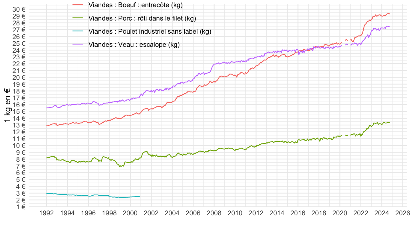
1996-
Value
Code
`IPC-PM-2015` %>%
  filter(PRIX_CONSO %in% c("1188", "1244", "1264", "1334"),
         FREQ == "M") %>%

  month_to_date() %>%
  filter(date >= as.Date("1996-01-01")) %>%
  ggplot + theme_minimal() + xlab("") + ylab("1 kg en €") +
  geom_line(aes(x = date, y = OBS_VALUE, color = Prix_conso)) +
  scale_x_date(breaks = seq(1960, 2100, 2) %>% paste0("-01-01") %>% as.Date,
               labels = date_format("%Y")) +
  scale_y_continuous(breaks = seq(0, 100, 1),
                     labels = dollar_format(accuracy = 1, prefix = "", su = " €")) +

  theme(legend.position = c(0.3, 0.9),
        legend.title = element_blank())
100
Code
`IPC-PM-2015` %>%
  filter(PRIX_CONSO %in% c("1188", "1244", "1264", "1334"),
         FREQ == "M") %>%

  month_to_date() %>%
  arrange(date) %>%
  filter(date >= as.Date("1996-01-01")) %>%
  group_by(PRIX_CONSO) %>%
  mutate(OBS_VALUE = 100*OBS_VALUE/OBS_VALUE[1]) %>%
  ggplot + theme_minimal() + xlab("") + ylab("") +
  geom_line(aes(x = date, y = OBS_VALUE, color = Prix_conso)) +
  scale_x_date(breaks = seq(1960, 2100, 2) %>% paste0("-01-01") %>% as.Date,
               labels = date_format("%Y")) +
  scale_y_log10(breaks = seq(100, 850, 10)) +

  theme(legend.position = c(0.25, 0.9),
        legend.title = element_blank())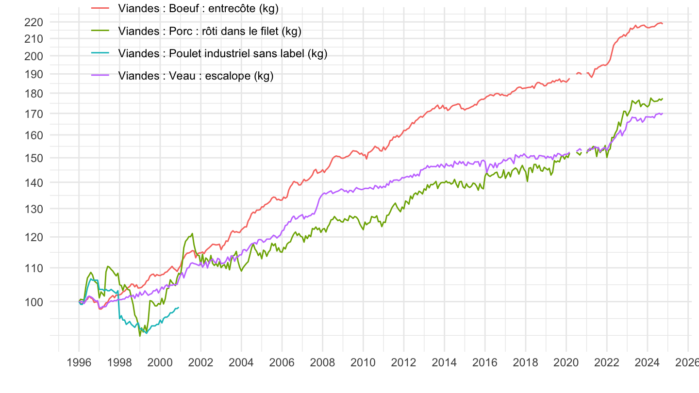
Apéritifs anisés, Whisky
1992
Code
`IPC-PM-2015` %>%
  filter(PRIX_CONSO %in% c("1180", "1181"),
         FREQ == "M") %>%

  month_to_date() %>%
  ggplot + theme_minimal() + xlab("") + ylab("en €") +
  geom_line(aes(x = date, y = OBS_VALUE, color = Prix_conso)) +
  scale_x_date(breaks = seq(1960, 2100, 2) %>% paste0("-01-01") %>% as.Date,
               labels = date_format("%Y")) +
  scale_y_continuous(breaks = seq(0, 100, 1),
                     labels = dollar_format(accuracy = 1, prefix = "", su = " €")) +

  theme(legend.position = c(0.3, 0.9),
        legend.title = element_blank())
1996-
Value
Code
`IPC-PM-2015` %>%
  filter(PRIX_CONSO %in% c("1180", "1181"),
         FREQ == "M") %>%

  month_to_date() %>%
  filter(date >= as.Date("1996-01-01")) %>%
  ggplot + theme_minimal() + xlab("") + ylab("1 kg en €") +
  geom_line(aes(x = date, y = OBS_VALUE, color = Prix_conso)) +
  scale_x_date(breaks = seq(1960, 2100, 2) %>% paste0("-01-01") %>% as.Date,
               labels = date_format("%Y")) +
  scale_y_continuous(breaks = seq(0, 100, 1),
                     labels = dollar_format(accuracy = 1, prefix = "", su = " €")) +

  theme(legend.position = c(0.3, 0.9),
        legend.title = element_blank())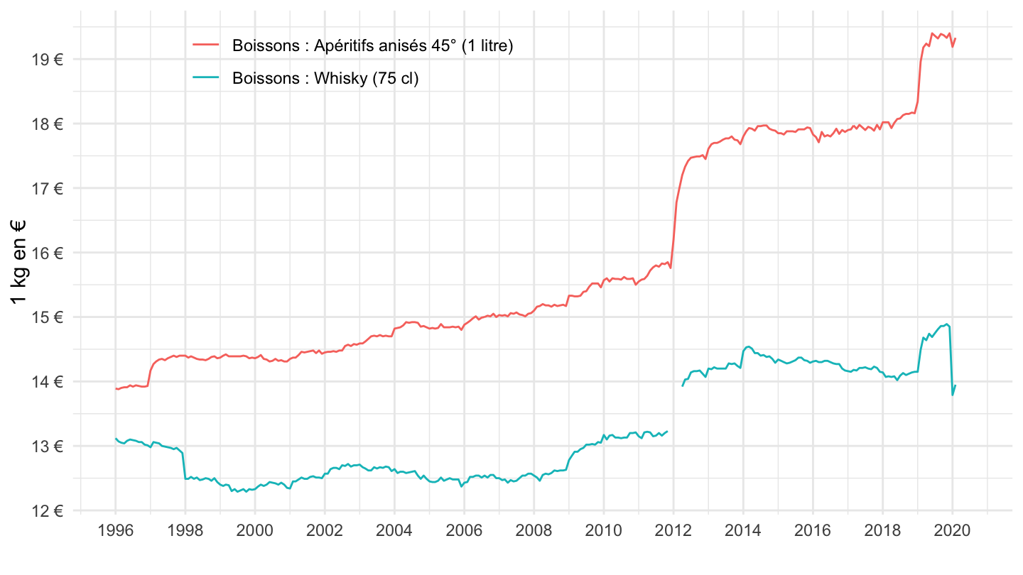
100
Code
`IPC-PM-2015` %>%
  filter(PRIX_CONSO %in% c("1180", "1181"),
         FREQ == "M") %>%

  month_to_date() %>%
  arrange(date) %>%
  filter(date >= as.Date("1996-01-01")) %>%
  group_by(PRIX_CONSO) %>%
  mutate(OBS_VALUE = 100*OBS_VALUE/OBS_VALUE[1]) %>%
  ggplot + theme_minimal() + xlab("") + ylab("") +
  geom_line(aes(x = date, y = OBS_VALUE, color = Prix_conso)) +
  scale_x_date(breaks = seq(1960, 2100, 2) %>% paste0("-01-01") %>% as.Date,
               labels = date_format("%Y")) +
  scale_y_log10(breaks = seq(100, 850, 10)) +

  theme(legend.position = c(0.25, 0.9),
        legend.title = element_blank())
2017-
Value
Code
`IPC-PM-2015` %>%
  filter(PRIX_CONSO %in% c("1180", "1181"),
         FREQ == "M") %>%

  month_to_date() %>%
  filter(date >= as.Date("2017-01-01")) %>%
  ggplot + theme_minimal() + xlab("") + ylab("1 kg en €") +
  geom_line(aes(x = date, y = OBS_VALUE, color = Prix_conso)) +
  scale_x_date(breaks = seq(1960, 2100, 1) %>% paste0("-01-01") %>% as.Date,
               labels = date_format("%Y")) +
  scale_y_continuous(breaks = seq(0, 100, 1),
                     labels = dollar_format(accuracy = 1, prefix = "", su = " €")) +

  theme(legend.position = c(0.3, 0.9),
        legend.title = element_blank())
100
Code
`IPC-PM-2015` %>%
  filter(PRIX_CONSO %in% c("1180", "1181"),
         FREQ == "M") %>%

  month_to_date() %>%
  arrange(date) %>%
  filter(date >= as.Date("2017-01-01")) %>%
  group_by(PRIX_CONSO) %>%
  mutate(OBS_VALUE = 100*OBS_VALUE/OBS_VALUE[1]) %>%
  ggplot + theme_minimal() + xlab("") + ylab("") +
  geom_line(aes(x = date, y = OBS_VALUE, color = Prix_conso)) +
  scale_x_date(breaks = seq(1960, 2100, 1) %>% paste0("-01-01") %>% as.Date,
               labels = date_format("%Y")) +
  scale_y_log10(breaks = seq(10, 850, 2)) +

  theme(legend.position = c(0.25, 0.9),
        legend.title = element_blank())
Services - Heures de M.O
Electricite, Plomberie
Code
`IPC-PM-2015` %>%
  filter(PRIX_CONSO %in% c("3077", "3078"),
         FREQ == "M") %>%

  month_to_date() %>%
  ggplot + theme_minimal() + xlab("") + ylab("1 kg en €") +
  geom_line(aes(x = date, y = OBS_VALUE, color = Prix_conso)) +
  scale_x_date(breaks = seq(1960, 2100, 2) %>% paste0("-01-01") %>% as.Date,
               labels = date_format("%Y")) +
  scale_y_continuous(breaks = seq(0, 100, 5),
                     labels = dollar_format(accuracy = 1, prefix = "", su = " €")) +

  theme(legend.position = c(0.3, 0.9),
        legend.title = element_blank())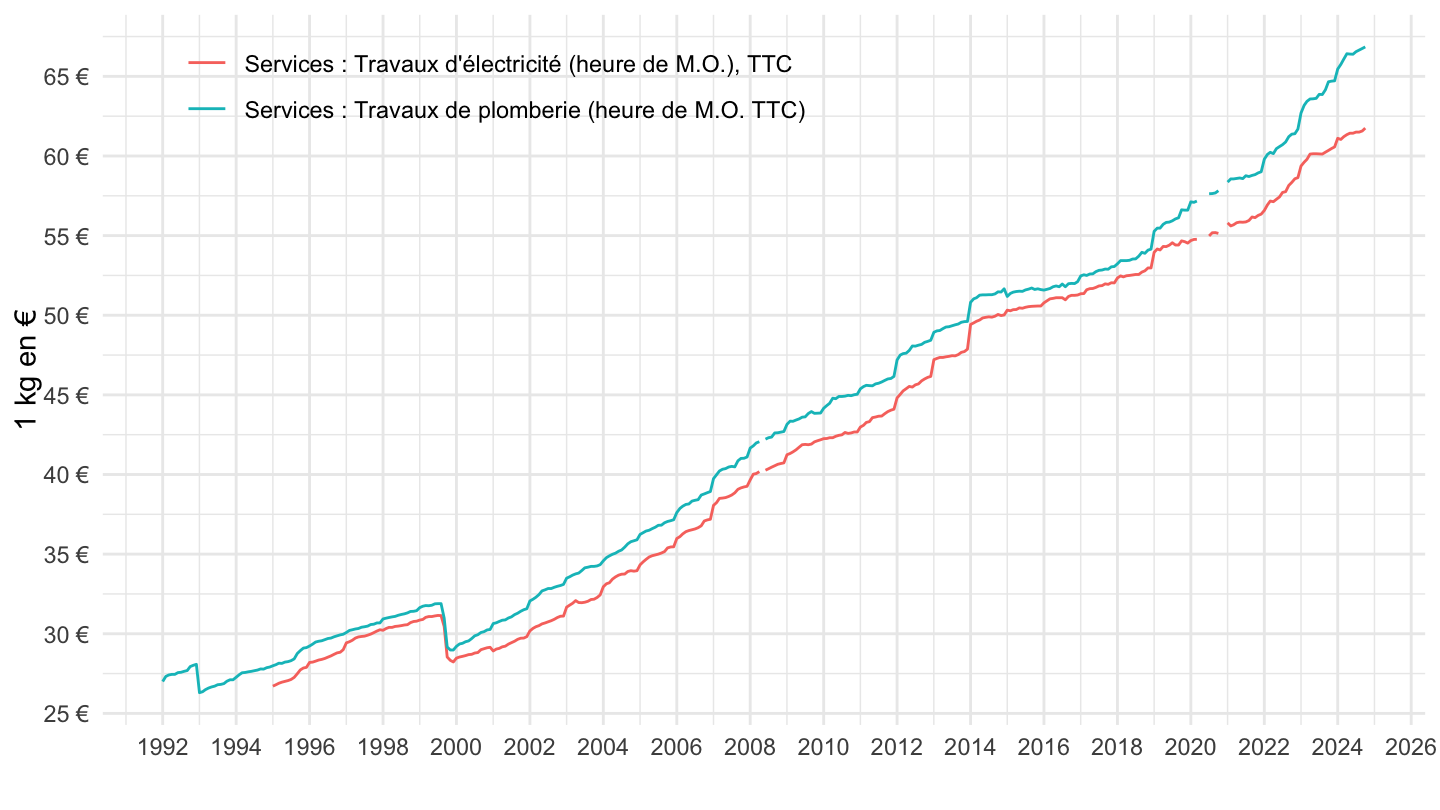
Carrosserie automobile, Mécanique automobile
Code
`IPC-PM-2015` %>%
  filter(PRIX_CONSO %in% c("2849", "2848"),
         FREQ == "M") %>%

  mutate(Prix_conso = gsub(" : une heure de main-d'oeuvre (y c. TVA)", "", Prix_conso)) %>%
  month_to_date() %>%
  ggplot + theme_minimal() + xlab("") + ylab("1 heure de M.O en €") +
  geom_line(aes(x = date, y = OBS_VALUE, color = Prix_conso)) +
  scale_x_date(breaks = seq(1960, 2100, 2) %>% paste0("-01-01") %>% as.Date,
               labels = date_format("%Y")) +
  scale_y_log10(breaks = seq(0, 100, 5),
                     labels = dollar_format(accuracy = 1, prefix = "", su = " €")) +

  theme(legend.position = c(0.65, 0.1),
        legend.title = element_blank())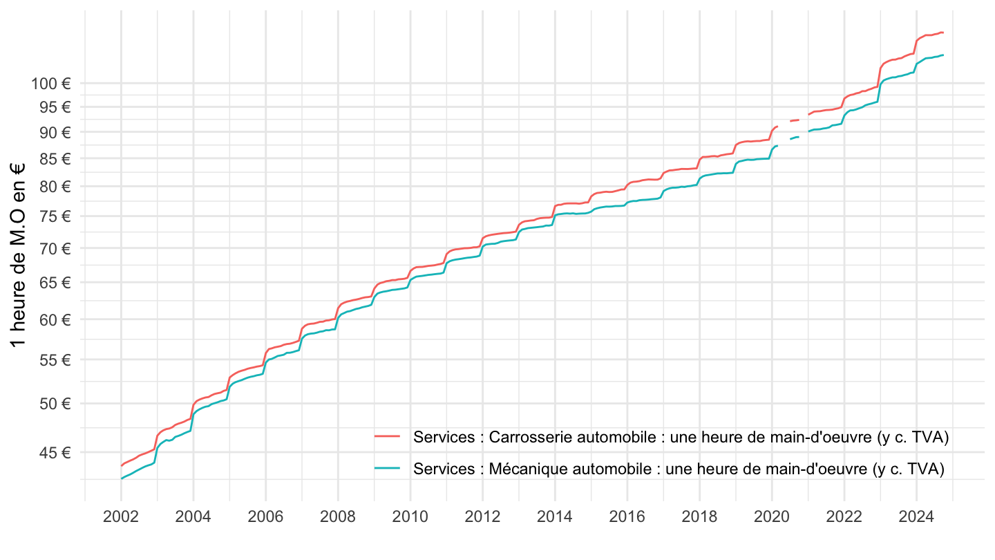
Shampooing
Code
`IPC-PM-2015` %>%
  filter(PRIX_CONSO %in% c("1932", "2326", "1930"),
         FREQ == "M") %>%

  month_to_date() %>%
  ggplot + theme_minimal() + xlab("") + ylab("") +
  geom_line(aes(x = date, y = OBS_VALUE, color = Prix_conso)) +
  scale_x_date(breaks = seq(1960, 2100, 2) %>% paste0("-01-01") %>% as.Date,
               labels = date_format("%Y")) +
  scale_y_log10(breaks = seq(0, 100, 5),
                     labels = dollar_format(accuracy = 1, prefix = "", su = " €")) +

  theme(legend.position = c(0.35, 0.9),
        legend.title = element_blank())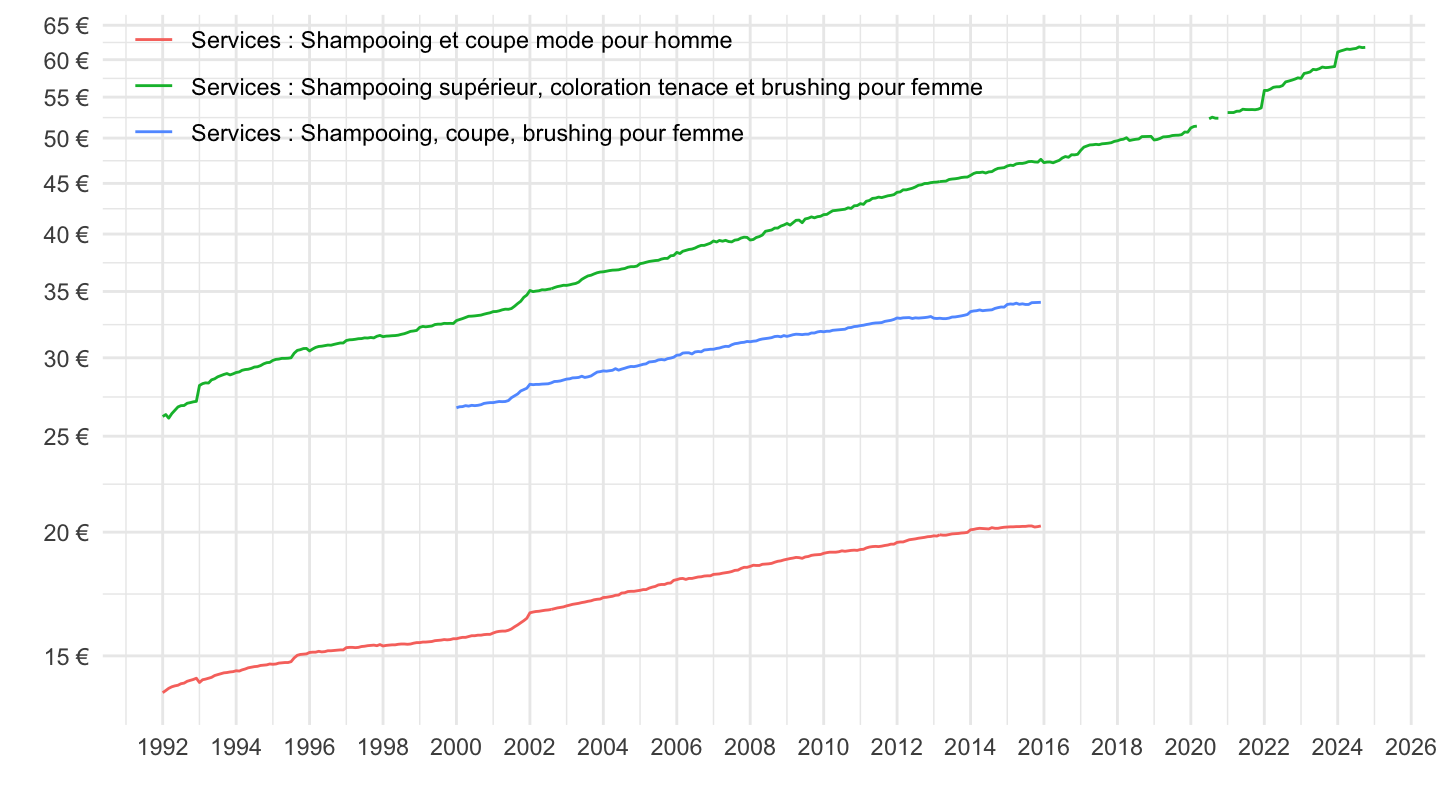
Services: Auto, Shampooing, Plomberie
2017-01
Code
`IPC-PM-2015` %>%
  filter(PRIX_CONSO %in% c("2849", "3078", "2848", "1932"),
         FREQ == "M") %>%

  month_to_date() %>%
  filter(date >= as.Date("2017-01-01")) %>%
  group_by(PRIX_CONSO) %>%
  arrange(date) %>%
  mutate(OBS_VALUE = 100*OBS_VALUE/OBS_VALUE[1]) %>%
  ggplot + theme_minimal() + xlab("") + ylab("Prix moyens, Services (100 = janvier 2017)") +
  geom_line(aes(x = date, y = OBS_VALUE, color = Prix_conso)) +
  scale_x_date(breaks = seq(1960, 2100, 1) %>% paste0("-01-01") %>% as.Date,
               labels = date_format("%Y")) +
  scale_y_continuous(breaks = seq(0, 300, 5)) +

  theme(legend.position = c(0.4, 0.85),
        legend.title = element_blank()) +
  geom_label_repel(data = . %>% filter(date == max(date)),
             aes(x = date, y = OBS_VALUE, color = Prix_conso, label = round(OBS_VALUE, 1)),
             show.legend = F)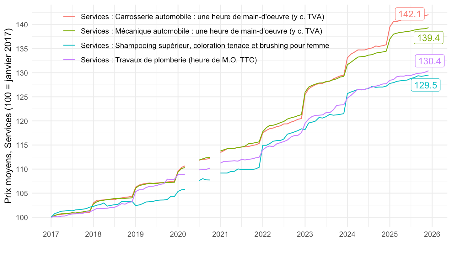
Bar / Restaurant
Café
Code
`IPC-PM-2015` %>%
  filter(PRIX_CONSO %in% c("2782", "2126"),
         FREQ == "M") %>%
  month_to_date() %>%

  ggplot + theme_minimal() + xlab("") + ylab("") +
  geom_line(aes(x = date, y = OBS_VALUE, color = Prix_conso)) +
  scale_x_date(breaks = seq(1960, 2100, 2) %>% paste0("-01-01") %>% as.Date,
               labels = date_format("%Y")) +
  scale_y_continuous(breaks = seq(0, 3, 0.1),
                     labels = dollar_format(accuracy = .1, prefix = "", su = " €")) +

  theme(legend.position = c(0.25, 0.9),
        legend.title = element_blank())
Cola, Bière
All
Code
`IPC-PM-2015` %>%
  filter(PRIX_CONSO %in% c("2433", "2768"),
         FREQ == "M") %>%
  month_to_date() %>%

  ggplot + theme_minimal() + xlab("") + ylab("") +
  geom_line(aes(x = date, y = OBS_VALUE, color = Prix_conso)) +
  scale_x_date(breaks = seq(1960, 2100, 2) %>% paste0("-01-01") %>% as.Date,
               labels = date_format("%Y")) +
  scale_y_continuous(breaks = seq(0, 7, 0.1),
                     labels = dollar_format(accuracy = .1, prefix = "", su = " €")) +

  theme(legend.position = c(0.25, 0.9),
        legend.title = element_blank())
2000-2004
Code
`IPC-PM-2015` %>%
  filter(PRIX_CONSO %in% c("2433", "2768"),
         FREQ == "M") %>%
  month_to_date() %>%
  filter(date >= as.Date("2000-01-01"),
         date <= as.Date("2004-01-01")) %>%

  ggplot + theme_minimal() + xlab("") + ylab("") +
  geom_line(aes(x = date, y = OBS_VALUE, color = Prix_conso)) +
  scale_x_date(breaks = "3 months",
               labels = date_format("%b %Y")) +
  scale_y_continuous(breaks = seq(0, 7, 0.1),
                     labels = dollar_format(accuracy = .1, prefix = "", su = " €")) +

  theme(legend.position = c(0.25, 0.9),
        legend.title = element_blank(),
        axis.text.x = element_text(angle = 45, vjust = 1, hjust = 1))
Fruits et Légumes
Kiwi, Pamplemousses, Avocat
Code
`IPC-PM-2015` %>%
  filter(PRIX_CONSO %in% c("3840", "3903", "3841"),
         FREQ == "M") %>%
  month_to_date() %>%

  ggplot + theme_minimal() + xlab("") + ylab("") +
  geom_line(aes(x = date, y = OBS_VALUE, color = Prix_conso)) +
  scale_x_date(breaks = seq(1960, 2100, 1) %>% paste0("-01-01") %>% as.Date,
               labels = date_format("%Y")) +
  scale_y_continuous(breaks = seq(0, 3, 0.1),
                     labels = dollar_format(accuracy = .1, prefix = "", su = " €")) +

  theme(legend.position = c(0.25, 0.9),
        legend.title = element_blank())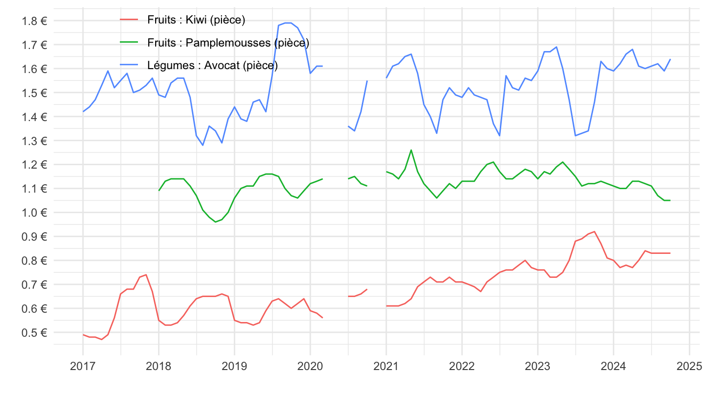
Bananes, Oranges, Carottes, Pomme de terre
Code
`IPC-PM-2015` %>%
  filter(PRIX_CONSO %in% c("8959", "8932", "8948", "8942"),
         FREQ == "M") %>%
  month_to_date() %>%

  ggplot + theme_minimal() + xlab("") + ylab("") +
  geom_line(aes(x = date, y = OBS_VALUE, color = Prix_conso)) +
  scale_x_date(breaks = seq(1960, 2100, 2) %>% paste0("-01-01") %>% as.Date,
               labels = date_format("%Y")) +
  scale_y_continuous(breaks = seq(0, 5, 0.2),
                     labels = dollar_format(accuracy = .1, prefix = "", su = " €")) +

  theme(legend.position = c(0.25, 0.9),
        legend.title = element_blank())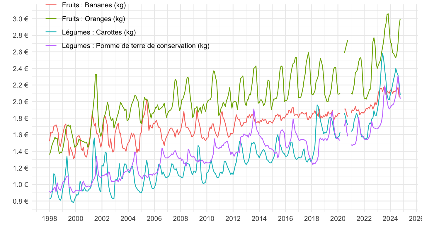
Pommes, Courgettes, Oignons, Tomates
Code
`IPC-PM-2015` %>%
  filter(PRIX_CONSO %in% c("8953", "8944", "8955", "8951"),
         FREQ == "M") %>%
  month_to_date() %>%

  ggplot + theme_minimal() + xlab("") + ylab("") +
  geom_line(aes(x = date, y = OBS_VALUE, color = Prix_conso)) +
  scale_x_date(breaks = seq(1960, 2100, 2) %>% paste0("-01-01") %>% as.Date,
               labels = date_format("%Y")) +
  scale_y_continuous(breaks = seq(0, 5, 0.2),
                     labels = dollar_format(accuracy = .1, prefix = "", su = " €")) +

  theme(legend.position = c(0.85, 0.9),
        legend.title = element_blank())