| source | dataset | Title | .html | .rData |
|---|---|---|---|---|
| eurostat | sts_inpp_m | Producer prices in industry, total - monthly data | 2026-07-20 | 2026-07-20 |
| eurostat | sts_inppd_m | Producer prices in industry, domestic market - monthly data | 2026-07-20 | 2026-07-20 |
| eurostat | sts_inppnd_m | Producer prices in industry, non domestic market - monthly data | 2026-07-20 | 2026-07-20 |
Producer prices in industry, total - monthly data
Data - Eurostat
Info
Last observation: Monthly: 2026M06 (N = 2,610)
First observation: Monthly: 1976M01 (N = 89)
Last data update: 21 jul 2026, 18:03. Last compile: 22 jul 2026, 00:28
Structure
Info
Code
include_graphics("https://ec.europa.eu/eurostat/statistics-explained/images/3/33/EU%2C_EA-19_Industrial_producer_prices%2C_total%2C_domestic_and_non-domestic_market%2C_2010_-_2022%2C_undadjusted_data_%282015_%3D_100%29_01-06-2022.png")
LAST_COMPILE
| LAST_COMPILE |
|---|
| 2026-07-22 |
Last
Code
sts_inpp_m %>%
  group_by(time) %>%
  summarise(Nobs = n()) %>%
  arrange(desc(time)) %>%
  head(1) %>%
print_table_conditional()| time | Nobs |
|---|---|
| 2026M06 | 2610 |
France, Germany, Italy
MIG_DCOG - MIG - durable consumer goods
Percentage change compared to same period in previous year - PCH_SM
All
Code
sts_inpp_m %>%
  filter(nace_r2 == "MIG_DCOG",
         indic_bt == "PRC_PRR",
         unit == "PCH_SM",
         geo %in% c("FR", "DE", "IT")) %>%
  transmute(geo, time, values = values/100) %>%
  left_join(geo, by = "geo") %>%
  left_join(colors, by = c("Geo" = "country")) %>%
  month_to_date %>%
  ggplot() + ylab("MIG_DCOG - MIG - durable consumer goods") + xlab("") + theme_minimal() +
  geom_line(aes(x = date, y = values, color = color)) +
  scale_color_identity() +
  scale_x_date(breaks = seq(1920, 2100, 2) %>% paste0("-01-01") %>% as.Date,
               labels = date_format("%Y")) +
  add_3flags +
  scale_y_continuous(breaks = 0.01*seq(-60, 300, 1),
                     labels = percent_format(a = 1))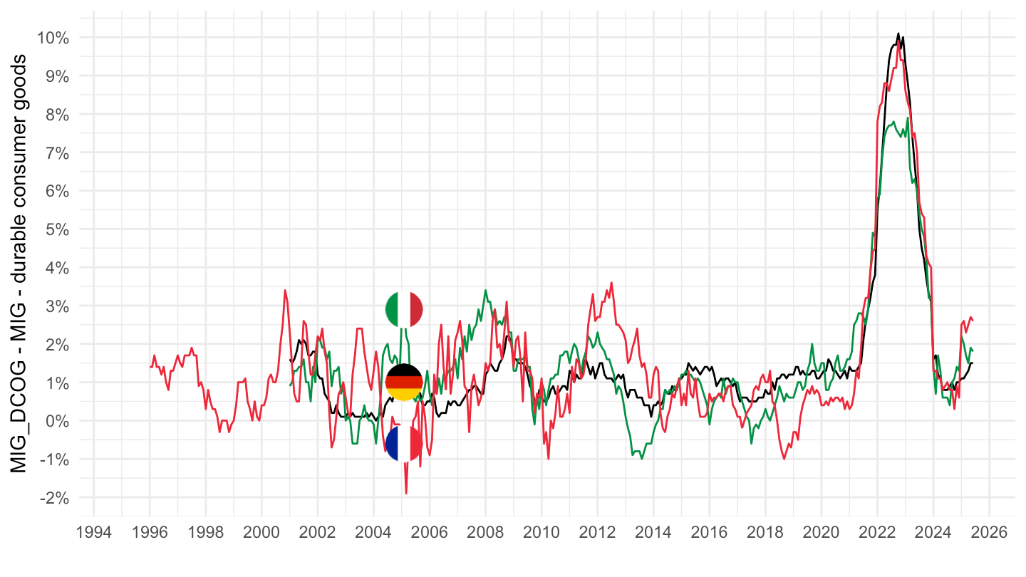
MIG_ING - MIG - intermediate goods
Percentage change compared to same period in previous year - PCH_SM
All
Code
sts_inpp_m %>%
  filter(nace_r2 == "MIG_ING",
         indic_bt == "PRC_PRR",
         unit == "PCH_SM",
         geo %in% c("FR", "DE", "IT")) %>%
  transmute(geo, time, values = values/100) %>%
  left_join(geo, by = "geo") %>%
  left_join(colors, by = c("Geo" = "country")) %>%
  month_to_date %>%
  ggplot() + ylab("MIG - intermediate goods") + xlab("") + theme_minimal() +
  geom_line(aes(x = date, y = values, color = color)) +
  scale_color_identity() +
  scale_x_date(breaks = seq(1920, 2100, 2) %>% paste0("-01-01") %>% as.Date,
               labels = date_format("%Y")) +
  add_3flags +
  scale_y_continuous(breaks = 0.01*seq(-60, 300, 1),
                     labels = percent_format(a = 1))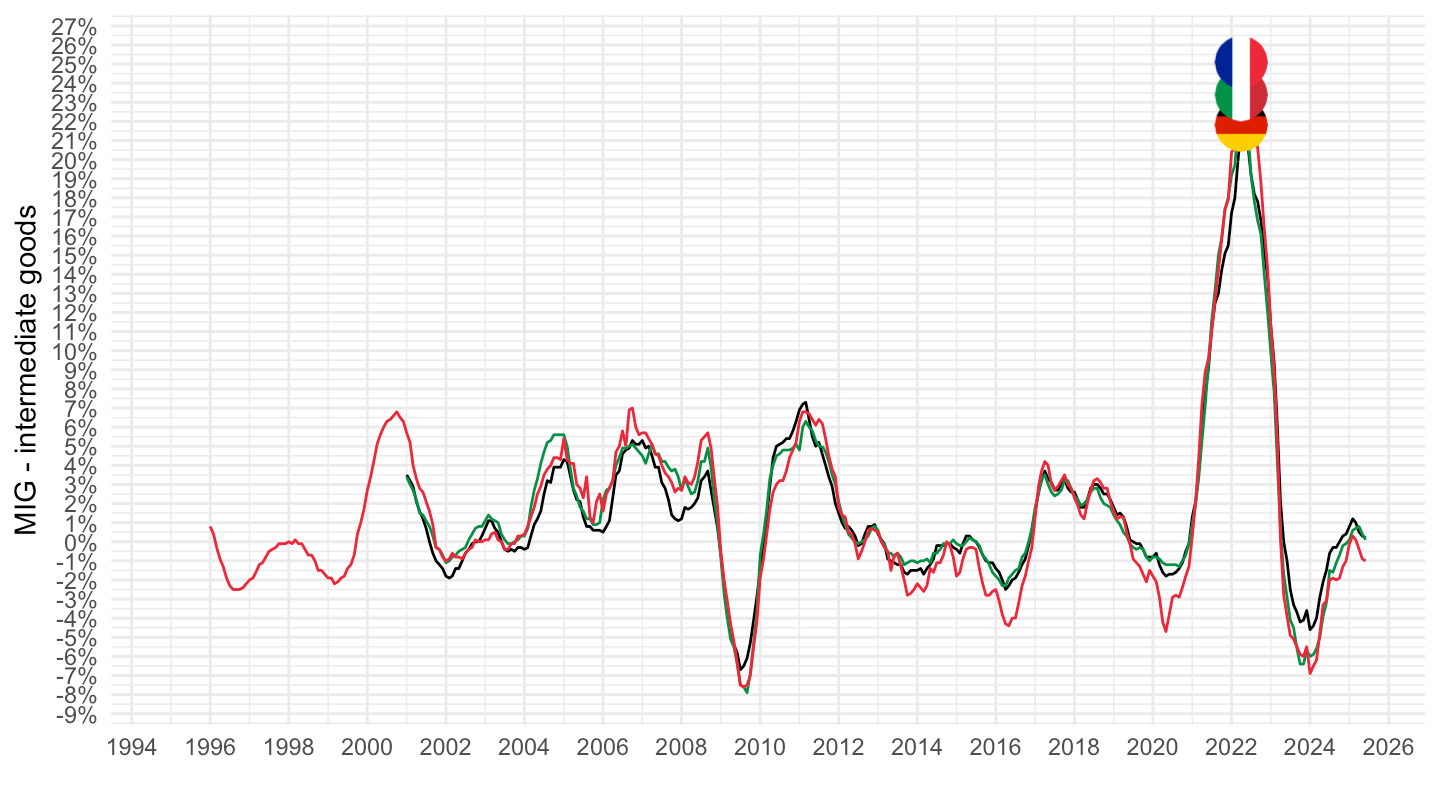
MIG_CAG - MIG - capital goods
Percentage change compared to same period in previous year - PCH_SM
All
Code
sts_inpp_m %>%
  filter(nace_r2 == "MIG_CAG",
         indic_bt == "PRC_PRR",
         unit == "PCH_SM",
         geo %in% c("FR", "DE", "IT")) %>%
  transmute(geo, time, values = values/100) %>%
  left_join(geo, by = "geo") %>%
  left_join(colors, by = c("Geo" = "country")) %>%
  month_to_date %>%
  ggplot() + ylab("MIG - capital goods") + xlab("") + theme_minimal() +
  geom_line(aes(x = date, y = values, color = color)) +
  scale_color_identity() +
  scale_x_date(breaks = seq(1920, 2100, 2) %>% paste0("-01-01") %>% as.Date,
               labels = date_format("%Y")) +
  add_3flags +
  scale_y_continuous(breaks = 0.01*seq(-60, 300, 1),
                     labels = percent_format(a = 1))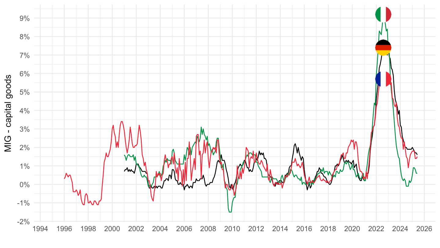
D - Electricity, gas, steam and air conditioning supply
Percentage change compared to same period in previous year - PCH_SM
All
Code
sts_inpp_m %>%
  filter(nace_r2 == "D",
         indic_bt == "PRC_PRR",
         unit == "PCH_SM",
         geo %in% c("FR", "DE", "IT")) %>%
  transmute(geo, time, values = values/100) %>%
  left_join(geo, by = "geo") %>%
  left_join(colors, by = c("Geo" = "country")) %>%
  month_to_date %>%
  ggplot() + ylab("Non-domestic output price index") + xlab("") + theme_minimal() +
  geom_line(aes(x = date, y = values, color = color)) +
  scale_color_identity() +
  scale_x_date(breaks = seq(1920, 2100, 2) %>% paste0("-01-01") %>% as.Date,
               labels = date_format("%Y")) +
  add_3flags +
  scale_y_continuous(breaks = 0.01*seq(-60, 300, 10),
                     labels = percent_format(a = 1))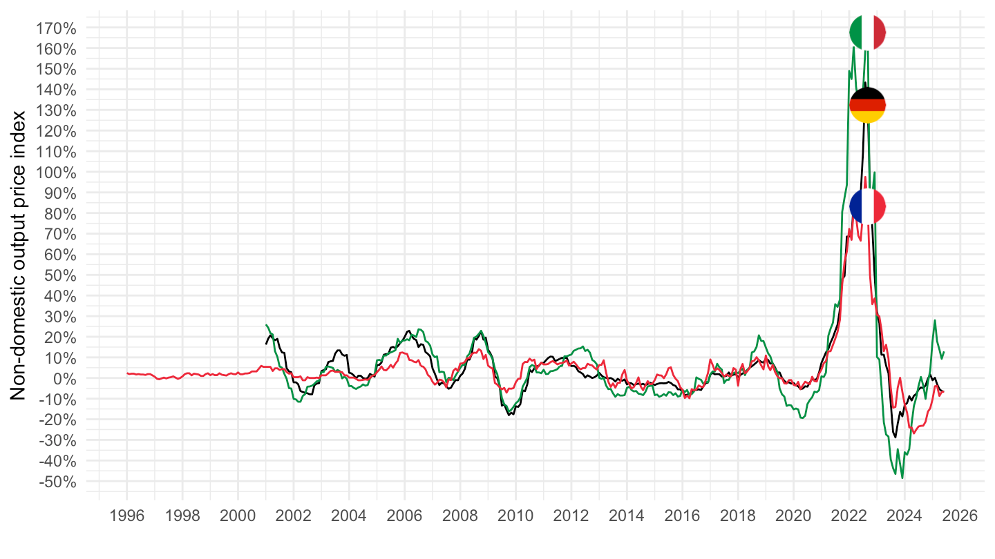
B - Mining and quarrying
Percentage change compared to same period in previous year - PCH_SM
All
Code
sts_inpp_m %>%
  filter(nace_r2 == "B",
         indic_bt == "PRC_PRR",
         unit == "PCH_SM",
         geo %in% c("FR", "DE", "IT")) %>%
  transmute(geo, time, values = values/100) %>%
  left_join(geo, by = "geo") %>%
  left_join(colors, by = c("Geo" = "country")) %>%
  month_to_date %>%
  ggplot() + ylab("Mining and quarrying") + xlab("") + theme_minimal() +
  geom_line(aes(x = date, y = values, color = color)) +
  scale_color_identity() +
  scale_x_date(breaks = seq(1920, 2100, 2) %>% paste0("-01-01") %>% as.Date,
               labels = date_format("%Y")) +
  add_3flags +
  scale_y_continuous(breaks = 0.01*seq(-60, 300, 10),
                     labels = percent_format(a = 1))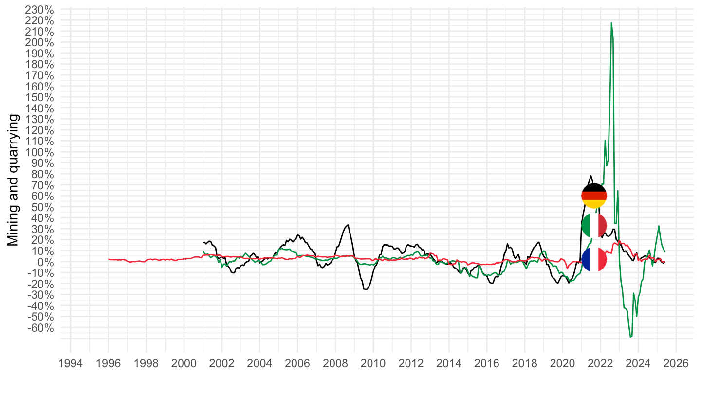
C - Manufacturing
Percentage change compared to same period in previous year - PCH_SM
All
Code
sts_inpp_m %>%
  filter(nace_r2 == "C",
         indic_bt == "PRC_PRR",
         unit == "PCH_SM",
         geo %in% c("FR", "DE", "IT")) %>%
  transmute(geo, time, values = values/100) %>%
  left_join(geo, by = "geo") %>%
  left_join(colors, by = c("Geo" = "country")) %>%
  month_to_date %>%
  ggplot() + ylab("% change compared to same period in previous year") + xlab("") + theme_minimal() +
  geom_line(aes(x = date, y = values, color = color)) +
  scale_color_identity() +
  scale_x_date(breaks = seq(1920, 2100, 2) %>% paste0("-01-01") %>% as.Date,
               labels = date_format("%Y")) +
  add_3flags +
  scale_y_continuous(breaks = 0.01*seq(-60, 300, 2),
                     labels = percent_format(a = 1))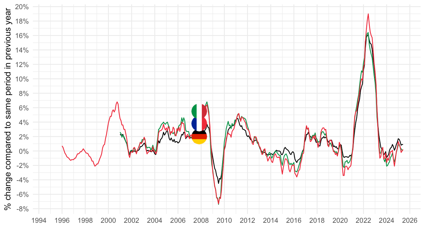
2000-
Code
sts_inpp_m %>%
  filter(nace_r2 == "C",
         indic_bt == "PRC_PRR",
         unit == "PCH_SM",
         geo %in% c("FR", "DE", "IT")) %>%
  transmute(geo, time, values = values/100) %>%
  left_join(geo, by = "geo") %>%
  left_join(colors, by = c("Geo" = "country")) %>%
  month_to_date %>%
  filter(date >= as.Date("2000-01-01")) %>%
  ggplot() + ylab("% change compared to same period in previous year") + xlab("") + theme_minimal() +
  geom_line(aes(x = date, y = values, color = color)) +
  scale_color_identity() +
  scale_x_date(breaks = seq(1920, 2100, 2) %>% paste0("-01-01") %>% as.Date,
               labels = date_format("%Y")) +
  add_3flags +
  scale_y_continuous(breaks = 0.01*seq(-60, 300, 2),
                     labels = percent_format(a = 1))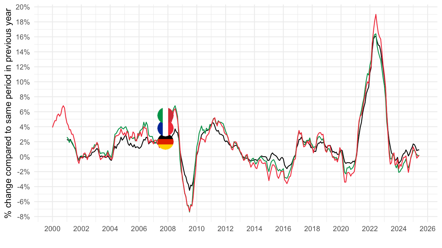
2018-
Code
sts_inpp_m %>%
  filter(nace_r2 == "C",
         indic_bt == "PRC_PRR",
         unit == "PCH_SM",
         geo %in% c("FR", "DE", "IT")) %>%
  transmute(geo, time, values = values/100) %>%
  left_join(geo, by = "geo") %>%
  left_join(colors, by = c("Geo" = "country")) %>%
  month_to_date %>%
  filter(date >= as.Date("2018-01-01")) %>%
  ggplot() + ylab("% change compared to same period in previous year") + xlab("") + theme_minimal() +
  geom_line(aes(x = date, y = values, color = color)) +
  scale_color_identity() +
  scale_x_date(breaks = seq(1920, 2100, 1) %>% paste0("-01-01") %>% as.Date,
               labels = date_format("%Y")) +
  add_3flags +
  scale_y_continuous(breaks = 0.01*seq(-60, 300, 2),
                     labels = percent_format(a = 1))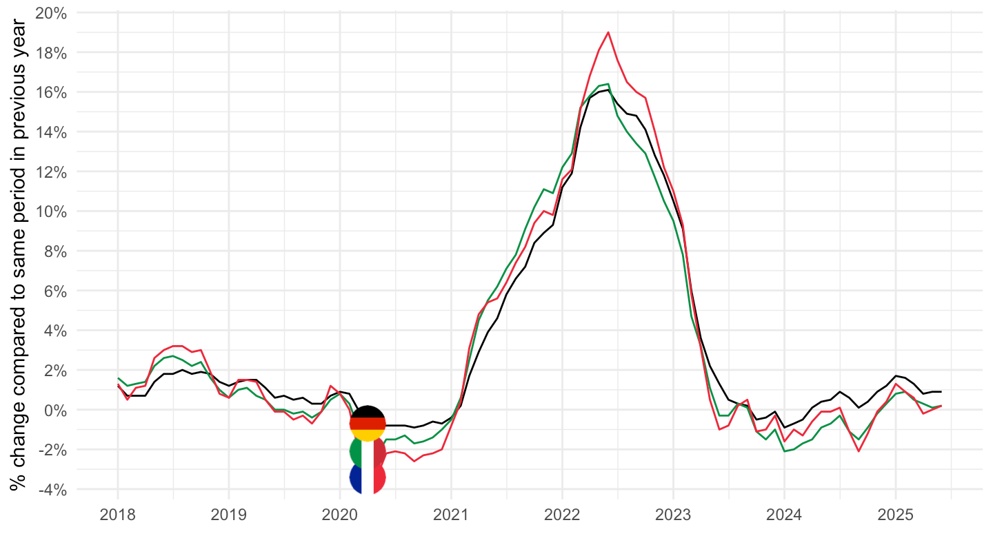
Index
All
Code
sts_inpp_m %>%
  filter(nace_r2 == "C",
         indic_bt == "PRC_PRR",
         unit == "I21",
         geo %in% c("FR", "DE", "IT")) %>%
  select(geo, time, values) %>%
  group_by(geo) %>%
  mutate(values = 100*values/values[time == "2000M01"]) %>%
  left_join(geo, by = "geo") %>%
  left_join(colors, by = c("Geo" = "country")) %>%
  month_to_date %>%
  ggplot() + ylab("Non-domestic output price index - in national currency") + xlab("") + theme_minimal() +
  geom_line(aes(x = date, y = values, color = color)) +
  scale_color_identity() +
  scale_x_date(breaks = seq(1920, 2100, 2) %>% paste0("-01-01") %>% as.Date,
               labels = date_format("%Y")) +
  add_3flags +
  theme(legend.position = "none") +
  scale_y_log10(breaks = seq(-60, 300, 10))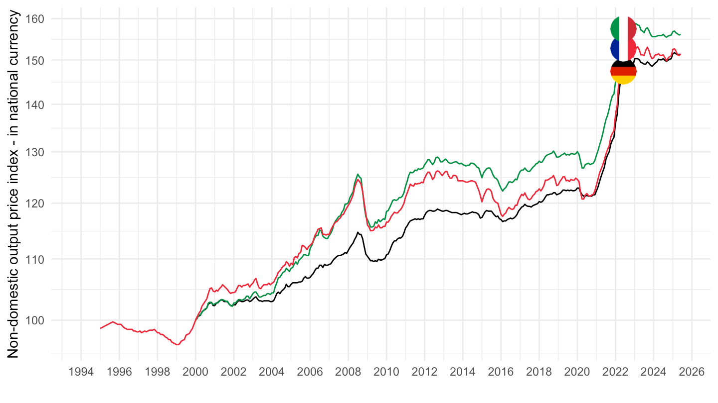
2000-
Code
sts_inpp_m %>%
  filter(nace_r2 == "C",
         indic_bt == "PRC_PRR",
         unit == "I21",
         geo %in% c("FR", "DE", "IT")) %>%
  select(geo, time, values) %>%
  group_by(geo) %>%
  mutate(values = 100*values/values[time == "2000M01"]) %>%
  left_join(geo, by = "geo") %>%
  left_join(colors, by = c("Geo" = "country")) %>%
  month_to_date %>%
  filter(date >= as.Date("2000-01-01")) %>%
  ggplot() + ylab("Total output price index - in national currency") + xlab("") + theme_minimal() +
  geom_line(aes(x = date, y = values, color = color)) +
  scale_color_identity() +
  scale_x_date(breaks = seq(1920, 2100, 2) %>% paste0("-01-01") %>% as.Date,
               labels = date_format("%y")) +
  add_3flags +
  theme(legend.position = "none") +
  scale_y_log10(breaks = seq(-60, 300, 5))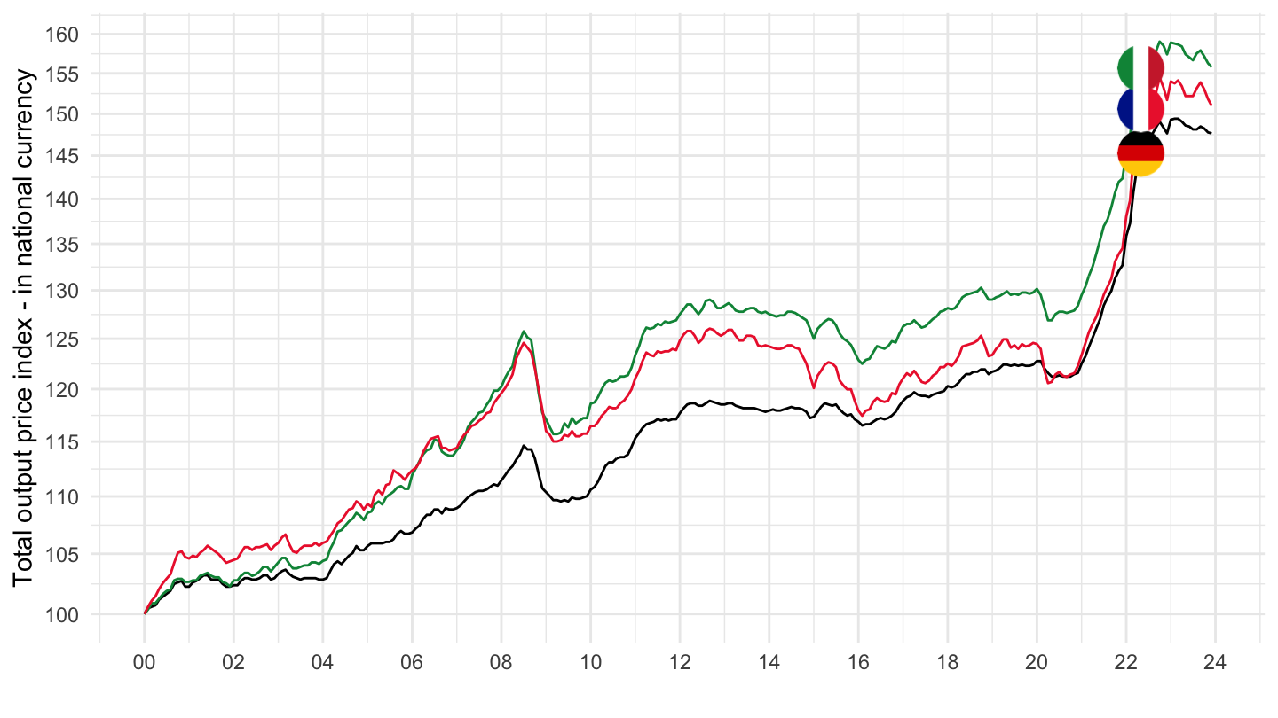
2015-
Code
sts_inpp_m %>%
  filter(nace_r2 == "C",
         indic_bt == "PRC_PRR",
         unit == "I21",
         geo %in% c("FR", "DE", "IT")) %>%
  select(geo, time, values) %>%
  group_by(geo) %>%
  mutate(values = 100*values/values[time == "2015M01"]) %>%
  left_join(geo, by = "geo") %>%
  left_join(colors, by = c("Geo" = "country")) %>%
  month_to_date %>%
  filter(date >= as.Date("2015-01-01")) %>%
  ggplot() + geom_line(aes(x = date, y = values, color = color)) + scale_color_identity() +
  add_3flags + ylab("Total output price index") + xlab("") + theme_minimal() +
  scale_x_date(breaks = seq(1920, 2100, 1) %>% paste0("-01-01") %>% as.Date,
               labels = date_format("%Y")) +
  scale_y_log10(breaks = seq(-60, 300, 5))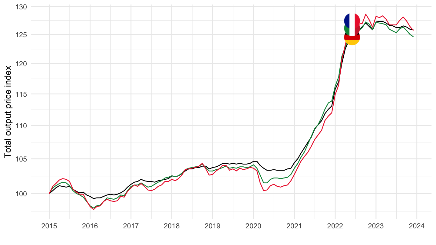
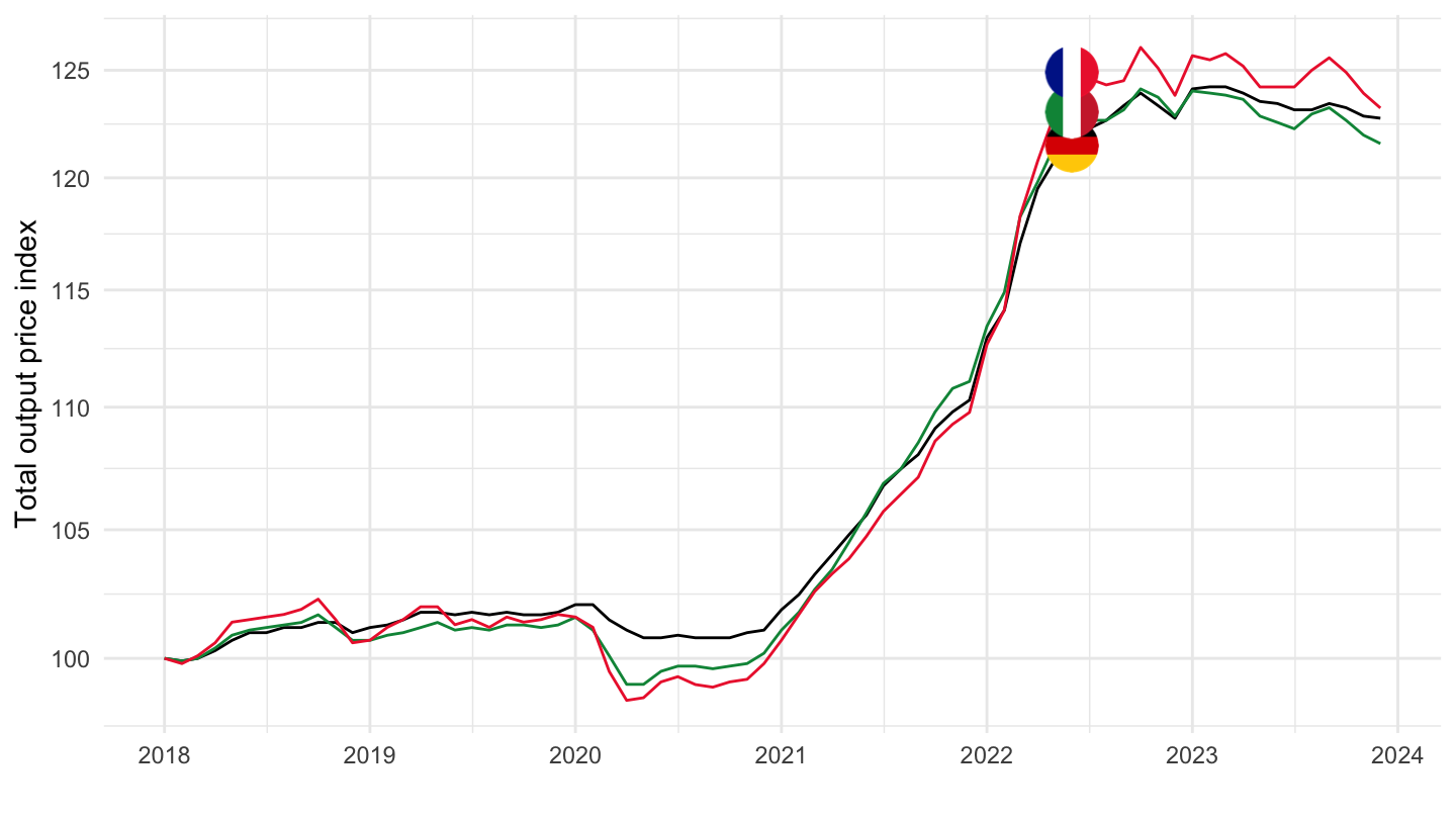
2018-
Code
sts_inpp_m %>%
  filter(nace_r2 == "C",
         indic_bt == "PRC_PRR",
         unit == "I21",
         geo %in% c("FR", "DE", "IT")) %>%
  select(geo, time, values) %>%
  group_by(geo) %>%
  mutate(values = 100*values/values[time == "2018M01"]) %>%
  left_join(geo, by = "geo") %>%
  left_join(colors, by = c("Geo" = "country")) %>%
  month_to_date %>%
  filter(date >= as.Date("2018-01-01")) %>%
  ggplot() + geom_line(aes(x = date, y = values, color = color)) + scale_color_identity() +
  add_3flags + ylab("Total output price index") + xlab("") + theme_minimal() +
  scale_x_date(breaks = seq(1920, 2100, 1) %>% paste0("-01-01") %>% as.Date,
               labels = date_format("%Y")) +
  scale_y_log10(breaks = seq(-60, 300, 5))