Mean consumption expenditure by income quintile - hbs_str_t223

Name: Mean consumption expenditure by income quintile
Creator: François Geerolf
License: https://creativecommons.org/licenses/by/4.0/

Data - Eurostat

Author

François Geerolf

Structure

coicop

France

Table

Code

hbs_str_t223 |>
  
  filter(geo == "FR",
         substr(coicop, 1, 2) == "CP",
         coicop != "CP00",
         time %in% c("2020")) |>
  select(-unit, -time) |>
  select(-geo) |>
  spread(quantile, values) |>
  print_table_conditional()

Sum

Code

hbs_str_t211 |>
  mutate(quantile = "TOTAL") |>
  bind_rows(hbs_str_t223) |>
  
  filter(geo == "FR",
         substr(coicop, 1, 2) == "CP",
         coicop != "CP00",
         time %in% c("2020")) |>
  mutate(coicop_nchar = nchar(coicop)) |>
  group_by(coicop_nchar, quantile) |>
  summarise(Nobs = n(),
            sum = sum(values)) |>
  print_table_conditional()

coicop_nchar	quantile	Nobs	sum
4	QUINTILE1	12	1000
4	QUINTILE2	12	1000
4	QUINTILE3	12	1001
4	QUINTILE4	12	999
4	QUINTILE5	12	1001
4	TOTAL	12	1002
5	QUINTILE1	47	993
5	QUINTILE2	47	992
5	QUINTILE3	47	993
5	QUINTILE4	47	988
5	QUINTILE5	47	981
5	TOTAL	47	991
6	TOTAL	115	896

2-digit and 3-digit

Code

`table1` <- hbs_str_t211 |>
  mutate(quantile = "TOTAL") |>
  bind_rows(hbs_str_t223) |>
  
  filter(geo == "FR",
         substr(coicop, 1, 2) == "CP",
         nchar(coicop) %in% c(4, 5),
         coicop != "CP00",
         time %in% c("2020")) |>
  select(-unit, -time) |>
  select(-geo) |>
  spread(quantile, values)

try(`table1` |>
  gt::gt() |>
  gt::gtsave(filename = "hbs_str_t223_files/figure-html/table1-1.png"))

`table1` |>
  print_table_conditional()

Missing: CP091+CP092+CP093+CP094 = 61 et pas 66

2-digit

Code

`table1-2digit` <- hbs_str_t211 |>
  mutate(quantile = "TOTAL") |>
  bind_rows(hbs_str_t223) |>
  
  filter(geo == "FR",
         substr(coicop, 1, 2) == "CP",
         nchar(coicop) == 4,
         coicop != "CP00",
         time %in% c("2020")) |>
  select(-unit, -time) |>
  select(-geo) |>
  spread(quantile, values)

try(`table1-2digit` |>
  gt::gt() |>
  gt::gtsave(filename = "hbs_str_t223_files/figure-html/table1-2digit-1.png"))

`table1-2digit` |>
  print_table_conditional()

coicop	Geo	Coicop	QUINTILE1	QUINTILE2	QUINTILE3	QUINTILE4	QUINTILE5	TOTAL
CP01	France	Food and non-alcoholic beverages	147	150	154	150	128	143
CP02	France	Alcoholic beverages, tobacco and narcotics	35	30	28	24	20	25
CP03	France	Clothing and footwear	43	37	38	39	41	40
CP04	France	Housing, water, electricity, gas and other fuels	347	328	305	279	255	289
CP05	France	Furnishings, household equipment and routine household maintenance	34	40	43	47	58	48
CP06	France	Health	15	16	18	16	15	16
CP07	France	Transport	102	113	121	139	149	132
CP08	France	Communications	35	28	25	23	18	24
CP09	France	Recreation and culture	66	66	72	76	89	77
CP10	France	Education	8	4	3	4	9	6
CP11	France	Restaurants and hotels	40	41	44	52	71	55
CP12	France	Miscellaneous goods and services	128	147	150	150	148	147

3-digit

Code

FR_3digit_weights2020 <- hbs_str_t211 |>
  mutate(quantile = "TOTAL") |>
  bind_rows(hbs_str_t223) |>
  filter(geo == "FR",
         substr(coicop, 1, 2) == "CP",
         nchar(coicop) == 5,
         coicop != "CP00",
         time %in% c("2020")) |>
  select(-unit, -geo, -time)

dir.create("hbs_str_t223_files/data-RData", showWarnings = FALSE, recursive = TRUE)
do.call(save, list("FR_3digit_weights2020", file = "hbs_str_t223_files/data-RData/FR_3digit_weights2020.RData"))

FR_3digit_weights2020 |>
  spread(quantile, values) |>
  print_table_conditional()

Code

try(FR_3digit_weights2020 |>
  spread(quantile, values) |>
  gt::gt() |>
  gt::gtsave(filename = "hbs_str_t223_files/figure-html/FR_3digit_weights2020-1.png"))

France - Compare

2020, HBS

Code

hbs_str_t223 |>
  filter(time == "2020",
         geo == "FR") %>%
  
  select_if(~ n_distinct(.) > 1) |>
  spread(quantile, values) %>%
  select_if(~ n_distinct(.) > 1) |>
  print_table_conditional()

2015, HBS

All

Code

hbs_str_t223 |>
  filter(time == "2015",
         geo == "FR") %>%
  
  select_if(~ n_distinct(.) > 1) |>
  spread(quantile, values) %>%
  select_if(~ n_distinct(.) > 1) |>
  print_table_conditional()

2-digit

Code

hbs_str_t223 |>
  filter(time == "2015",
         geo == "FR",
         nchar(coicop) == 4) %>%
  
  select_if(~ n_distinct(.) > 1) |>
  spread(quantile, values) %>%
  select_if(~ n_distinct(.) > 1) |>
  print_table_conditional()

coicop	Coicop	QUINTILE1	QUINTILE2	QUINTILE3	QUINTILE4	QUINTILE5
CP01	Food and non-alcoholic beverages	147	150	154	150	128
CP02	Alcoholic beverages, tobacco and narcotics	35	30	28	24	20
CP03	Clothing and footwear	43	37	38	39	41
CP04	Housing, water, electricity, gas and other fuels	347	328	305	279	255
CP05	Furnishings, household equipment and routine household maintenance	34	40	43	47	58
CP06	Health	15	16	18	16	15
CP07	Transport	102	113	121	139	149
CP08	Communications	35	28	25	23	18
CP09	Recreation and culture	66	66	72	76	89
CP10	Education	8	4	3	4	9
CP11	Restaurants and hotels	40	41	44	52	71
CP12	Miscellaneous goods and services	128	147	150	150	148

France

Actual + Imputed

Code

hbs_str_t223 |>
  filter(coicop %in% c("CP041", "CP042"),
         time == "2015",
         geo %in% c("FR")) |>
  mutate(Coicop = factor(coicop, levels = c("CP042", "CP041"), labels = c("Loyers imputés (propriétaires)", "Loyers réels (locataires)"))) |>
  ggplot() + geom_col(aes(x = quantile, y = values/1000, fill = Coicop)) +
  theme_minimal() +
  xlab("Quintile") + ylab("Poids dans l'Indice des Prix") +
  scale_y_continuous(breaks = 0.01*seq(-30, 50, 5),
                     labels = percent_format(accuracy = 1)) +
  theme(legend.position = "top",
        legend.direction = "horizontal",
        legend.title = element_blank())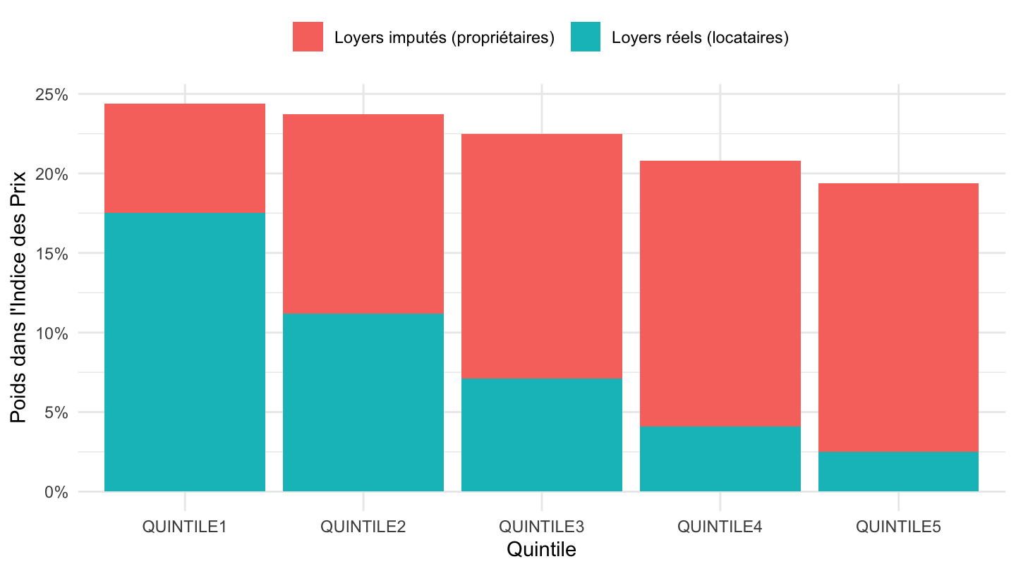

Tous

Code

hbs_str_t225 |>
  rename(category = age) |>
  mutate(type = "age") |>
  bind_rows(hbs_str_t223 |>
              rename(category = quantile) |>
              mutate(type = "quantile")) |>
  bind_rows(hbs_str_t226 |>
              rename(category = deg_urb) |>
              mutate(type = "deg_urb")) |>
  filter(coicop %in% c("CP041", "CP042"),
         time == "2015",
         geo %in% c("FR")) |>
  mutate(Coicop = factor(coicop, levels = c("CP042", "CP041"), labels = c("Loyers imputés (propriétaires)", "Loyers réels (locataires)")),
         Category = factor(category, levels = c("Y_LT30", "Y30-44", "Y45-59", "Y_GE60",
                                                "DEG1", "DEG2", "DEG3",
                                                "QUINTILE1", "QUINTILE2", "QUINTILE3", "QUINTILE4", "QUINTILE5"),
                           labels = c("Moins de 30 ans", "De 30 à 44 ans", "De 45 à 59 ans", "Plus de 60 ans",
                                      "Villes", "Villes - peuplées\net banlieues", "Zones rurales",
                                      "1er", "2è", "3è", "4è", "5è")),
         Type = factor(type, levels = c("age", "deg_urb", "quantile"),
                       labels = c("Age", "Commune de résidence", "Cinquième"))) |>
  ggplot() + geom_col(aes(x = Category, y = values/1000, fill = Coicop)) +
  theme_minimal() +
  xlab("") + ylab("Poids dans l'Indice des Prix") +
  scale_y_continuous(breaks = 0.01*seq(-30, 50, 5),
                     labels = percent_format(accuracy = 1)) +
  theme(legend.position = "top",
        legend.direction = "horizontal",
        legend.title = element_blank(),
        axis.text.x = element_text(angle = 45, vjust = 1, hjust = 1)) +
  facet_wrap(~ Type, scales = "free")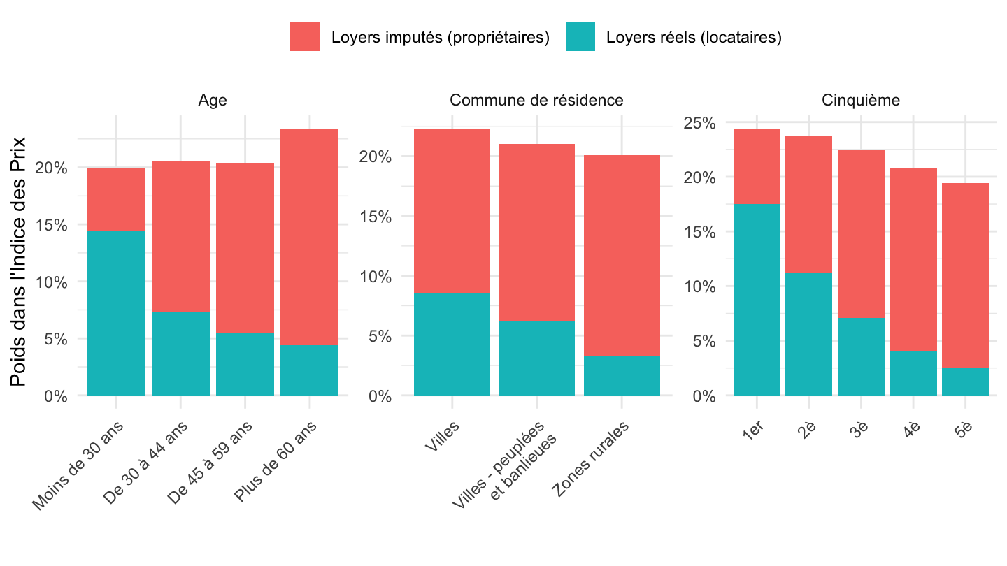

All quintiles

Sums

2-digit

Code

hbs_str_t223 |>
  filter(time == "2020",
         substr(coicop, 1, 2) == "CP",
         nchar(coicop) == 4) %>%
  
  select_if(~ n_distinct(.) > 1) |>
  group_by(quantile, geo, Geo) |>
  summarise(values = sum(values)) |>
  spread(quantile, values) |>
  print_table_conditional()

geo	Geo	QUINTILE1	QUINTILE2	QUINTILE3	QUINTILE4	QUINTILE5
AT	Austria	1000	1001	998	1001	1001
BE	Belgium	1001	999	999	998	1000
BG	Bulgaria	999	1000	999	1000	999
CY	Cyprus	1001	1000	1000	1000	1000
DE	Germany	1000	1002	1000	1001	1001
DK	Denmark	1001	999	1002	1000	1001
EE	Estonia	1001	1000	1000	999	1001
EL	Greece	999	1000	1001	999	1000
ES	Spain	1000	999	1002	1000	1000
EU27_2020	European Union - 27 countries (from 2020)	998	999	999	1000	1000
FI	Finland	999	1000	1000	998	1000
FR	France	1000	1000	1001	999	1001
HR	Croatia	998	999	1000	1000	1000
HU	Hungary	999	1000	1000	1000	999
IE	Ireland	999	1000	1001	1000	1000
LT	Lithuania	1001	1001	999	998	1001
LU	Luxembourg	1001	1001	999	1000	1000
LV	Latvia	999	1002	1001	1000	1000
ME	Montenegro	1001	1000	999	1000	1001
MT	Malta	1000	998	1002	1000	999
NL	Netherlands	1000	999	1000	1000	999
NO	Norway	999	1000	999	1000	999
PL	Poland	1001	1000	1001	1001	1001
PT	Portugal	1000	1001	1000	1000	999
RO	Romania	1000	1001	999	999	1000
RS	Serbia	999	999	1001	1000	1000
SI	Slovenia	1000	1000	1000	1000	999
SK	Slovakia	1001	1000	999	1000	1001
TR	Türkiye	1000	999	999	999	1000

3-digit

Code

hbs_str_t223 |>
  filter(time == "2020",
         substr(coicop, 1, 2) == "CP",
         nchar(coicop) == 5) %>%
  
  select_if(~ n_distinct(.) > 1) |>
  group_by(quantile, geo, Geo) |>
  summarise(values = sum(values)) |>
  spread(quantile, values) |>
  print_table_conditional()

geo	Geo	QUINTILE1	QUINTILE2	QUINTILE3	QUINTILE4	QUINTILE5
AT	Austria	996	1001	999	1001	1000
BE	Belgium	1000	1002	999	1001	998
BG	Bulgaria	1001	1002	998	1000	1000
CY	Cyprus	999	995	996	997	997
DE	Germany	994	992	992	995	986
DK	Denmark	1000	998	999	998	1000
EE	Estonia	980	982	984	986	988
EL	Greece	997	999	1002	999	1000
ES	Spain	1000	999	999	1000	999
FI	Finland	989	987	985	976	974
FR	France	993	992	993	988	981
HR	Croatia	1000	998	997	1004	1000
HU	Hungary	1000	1000	996	1000	999
IE	Ireland	1002	1000	999	1000	1000
LT	Lithuania	998	1002	1001	1000	1001
LU	Luxembourg	1001	997	996	998	1001
LV	Latvia	998	999	1001	998	1002
ME	Montenegro	986	985	987	981	985
MT	Malta	998	1004	997	1002	1001
NL	Netherlands	1001	998	1000	1000	1001
NO	Norway	984	993	997	998	993
PL	Poland	999	999	1003	1001	1001
RS	Serbia	998	998	999	1000	999
SI	Slovenia	1002	997	996	1000	1001
SK	Slovakia	998	997	1002	997	999
TR	Türkiye	1000	1000	995	1004	998

CP041, CP042, CP041_042

2015

Germany, France, Spain

Code

hbs_str_t223 |>
  filter(coicop %in% c("CP041", "CP042"),
         time == "2015",
         geo %in% c("ES", "FR", "DE")) |>
  select(coicop, geo, Geo, quantile, values) |>
  spread(coicop, values) |>
  mutate(CP041_042 = CP041 + CP042) |>
  gather(coicop, values, CP041, CP042, CP041_042) |>
  mutate(quantile = substr(quantile, 9, 9) |> as.numeric()) |>
  left_join(coicop_lab, by = "coicop") |>
  add_flag_color("Geo") |>
  mutate(Coicop = ifelse(coicop == "CP041_042", "Imputed rentals plus actual rentals", Coicop)) |>
  ggplot() + geom_line(aes(x = quantile, y = values/1000, color = color, linetype = Coicop)) +
  scale_color_identity() + theme_minimal() +
  geom_image(data = . %>%
               filter(quantile == 1) %>%
               mutate(image = paste0("../../icon/flag/round/", str_to_lower(gsub(" ", "-", Geo)), ".png")),
             aes(x = quantile, y = values/1000, image = image), asp = 1.5) +
  xlab("Quintile") + ylab("Weight in CPI") +
  scale_y_continuous(breaks = 0.01*seq(-30, 50, 5),
                     labels = percent_format(accuracy = 1)) +
  theme(legend.position = c(0.8, 0.9),
        legend.title = element_blank()) +
  scale_x_continuous(breaks = seq(0, 5, 1))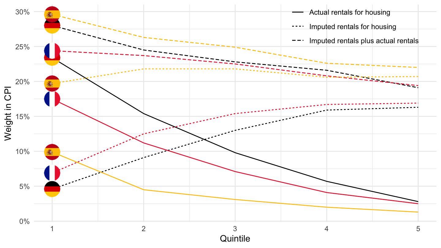

Netherlands, Austria, Greece

Code

hbs_str_t223 |>
  filter(coicop %in% c("CP041", "CP042"),
         time == "2015",
         geo %in% c("EL", "NL", "AT")) |>
  select(coicop, geo, Geo, quantile, values) |>
  spread(coicop, values) |>
  mutate(CP041_042 = CP041 + CP042) |>
  gather(coicop, values, CP041, CP042, CP041_042) |>
  mutate(quantile = substr(quantile, 9, 9) |> as.numeric()) |>
  left_join(coicop_lab, by = "coicop") |>
  add_flag_color("Geo") |>
  mutate(Coicop = ifelse(coicop == "CP041_042", "Imputed rentals plus actual rentals", Coicop)) |>
  ggplot() + geom_line(aes(x = quantile, y = values/1000, color = color, linetype = Coicop)) +
  scale_color_identity() + theme_minimal() +
  geom_image(data = . %>%
               filter(quantile == 1) %>%
               mutate(image = paste0("../../icon/flag/round/", str_to_lower(gsub(" ", "-", Geo)), ".png")),
             aes(x = quantile, y = values/1000, image = image), asp = 1.5) +
  xlab("Quintile") + ylab("Weight in CPI") +
  scale_y_continuous(breaks = 0.01*seq(-30, 50, 5),
                     labels = percent_format(accuracy = 1)) +
  theme(legend.position = c(0.8, 0.9),
        legend.title = element_blank()) +
  scale_x_continuous(breaks = seq(0, 5, 1))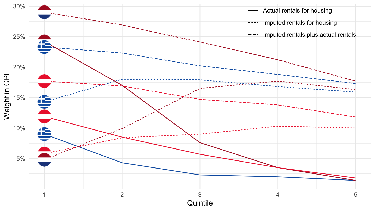

CP041, CP042

2015

All

Code

hbs_str_t223 |>
  filter(coicop %in% c("CP041", "CP042"),
         time == "2020") |>
  
  spread(quantile, values) %>%
  select_if(~ n_distinct(.) > 1) |>
  arrange(Geo) |>
  print_table_conditional()

Germany, France, Spain

Code

hbs_str_t223 |>
  filter(coicop %in% c("CP041", "CP042"),
         time == "2015",
         geo %in% c("ES", "FR", "DE")) |>
  mutate(quantile = substr(quantile, 9, 9) |> as.numeric()) |>
  
  
  add_flag_color("Geo") |>
  ggplot() + geom_line(aes(x = quantile, y = values/1000, color = color, linetype = Coicop)) +
  scale_color_identity() + theme_minimal() +
  geom_image(data = . %>%
               filter(quantile == 1) %>%
               mutate(image = paste0("../../icon/flag/round/", str_to_lower(gsub(" ", "-", Geo)), ".png")),
             aes(x = quantile, y = values/1000, image = image), asp = 1.5) +
  xlab("Quintile") + ylab("Weight in CPI") +
  scale_y_continuous(breaks = 0.01*seq(-30, 50, 5),
                     labels = percent_format(accuracy = 1)) +
  theme(legend.position = c(0.85, 0.85),
        legend.title = element_blank()) +
  scale_x_continuous(breaks = seq(0, 5, 1))

Netherlands, Austria, Greece

Code

hbs_str_t223 |>
  filter(coicop %in% c("CP041", "CP042"),
         time == "2015",
         geo %in% c("EL", "NL", "AT")) |>
  mutate(quantile = substr(quantile, 9, 9) |> as.numeric()) |>
  
  
  add_flag_color("Geo") |>
  ggplot() + geom_line(aes(x = quantile, y = values/1000, color = color, linetype = Coicop)) +
  scale_color_identity() + theme_minimal() +
  geom_image(data = . %>%
               filter(quantile == 1) %>%
               mutate(image = paste0("../../icon/flag/round/", str_to_lower(gsub(" ", "-", Geo)), ".png")),
             aes(x = quantile, y = values/1000, image = image), asp = 1.5) +
  xlab("Quintile") + ylab("Weight in CPI") +
  scale_y_continuous(breaks = 0.01*seq(-30, 50, 5),
                     labels = percent_format(accuracy = 1)) +
  theme(legend.position = c(0.8, 0.8),
        legend.title = element_blank()) +
  scale_x_continuous(breaks = seq(0, 5, 1))

2020

All

Code

hbs_str_t223 |>
  filter(coicop %in% c("CP041", "CP042"),
         time == "2020") |>
  
  spread(quantile, values) %>%
  select_if(~ n_distinct(.) > 1) |>
  arrange(Geo) |>
  print_table_conditional()

Germany, France, Spain

Code

hbs_str_t223 |>
  filter(coicop %in% c("CP041", "CP042"),
         time == "2020",
         geo %in% c("ES", "FR", "DE")) |>
  mutate(quantile = substr(quantile, 9, 9) |> as.numeric()) |>
  
  
  add_flag_color("Geo") |>
  ggplot() + geom_line(aes(x = quantile, y = values/1000, color = color, linetype = Coicop)) +
  scale_color_identity() + theme_minimal() +
  geom_image(data = . %>%
               filter(quantile == 1) %>%
               mutate(image = paste0("../../icon/flag/round/", str_to_lower(gsub(" ", "-", Geo)), ".png")),
             aes(x = quantile, y = values/1000, image = image), asp = 1.5) +
  xlab("Quintile") + ylab("Weight in CPI") +
  scale_y_continuous(breaks = 0.01*seq(-30, 50, 5),
                     labels = percent_format(accuracy = 1)) +
  theme(legend.position = c(0.8, 0.8),
        legend.title = element_blank()) +
  scale_x_continuous(breaks = seq(0, 5, 1))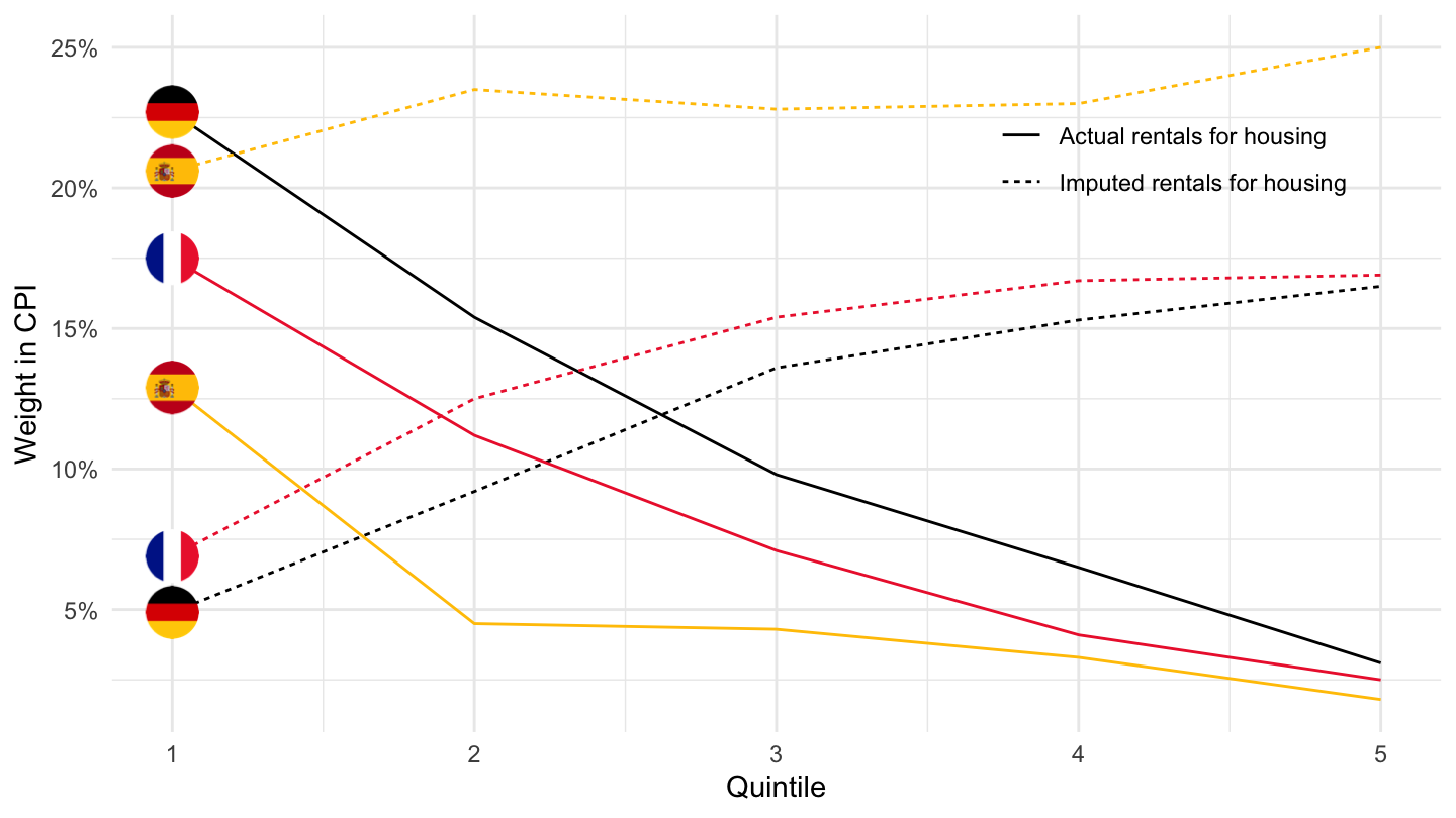

Netherlands, Austria, Greece

Code

hbs_str_t223 |>
  filter(coicop %in% c("CP041", "CP042"),
         time == "2020",
         geo %in% c("EL", "NL", "AT")) |>
  mutate(quantile = substr(quantile, 9, 9) |> as.numeric()) |>
  
  
  add_flag_color("Geo") |>
  ggplot() + geom_line(aes(x = quantile, y = values/1000, color = color, linetype = Coicop)) +
  scale_color_identity() + theme_minimal() +
  geom_image(data = . %>%
               filter(quantile == 1) %>%
               mutate(image = paste0("../../icon/flag/round/", str_to_lower(gsub(" ", "-", Geo)), ".png")),
             aes(x = quantile, y = values/1000, image = image), asp = 1.5) +
  xlab("Quintile") + ylab("Weight in CPI") +
  scale_y_continuous(breaks = 0.01*seq(-30, 50, 5),
                     labels = percent_format(accuracy = 1)) +
  theme(legend.position = c(0.85, 0.85),
        legend.title = element_blank()) +
  scale_x_continuous(breaks = seq(0, 5, 1))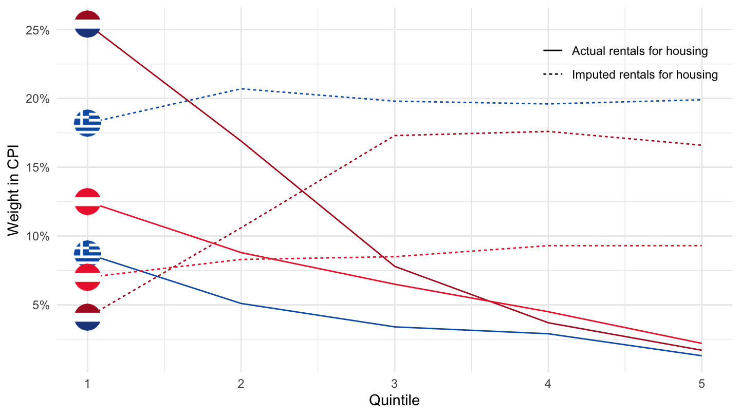

CP011, CP012

2015

All

Code

hbs_str_t223 |>
  filter(coicop %in% c("CP011", "CP012"),
         time == "2020") |>
  
  spread(quantile, values) %>%
  select_if(~ n_distinct(.) > 1) |>
  arrange(Geo) |>
  print_table_conditional()

Germany, France, Spain

All

Code

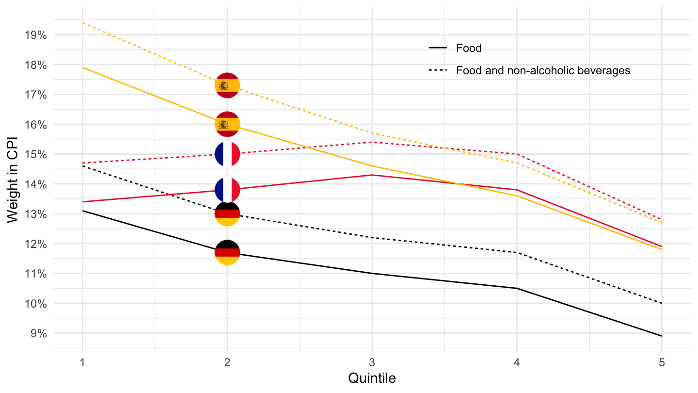
hbs_str_t223 |>
  filter(coicop %in% c("CP011", "CP01"),
         time == "2015",
         geo %in% c("ES", "FR", "DE")) |>
  mutate(quantile = substr(quantile, 9, 9) |> as.numeric()) |>
  
  
  add_flag_color("Geo") |>
  ggplot() + geom_line(aes(x = quantile, y = values/1000, color = color, linetype = Coicop)) +
  scale_color_identity() + theme_minimal() +
  geom_image(data = . %>%
               filter(quantile == 2) %>%
               mutate(image = paste0("../../icon/flag/round/", str_to_lower(gsub(" ", "-", Geo)), ".png")),
             aes(x = quantile, y = values/1000, image = image), asp = 1.5) +
  xlab("Quintile") + ylab("Weight in CPI") +
  scale_y_continuous(breaks = 0.01*seq(-30, 50, 1),
                     labels = percent_format(accuracy = 1)) +
  theme(legend.position = c(0.75, 0.85),
        legend.title = element_blank()) +
  scale_x_continuous(breaks = seq(0, 5, 1))

Related Data

Housing Market Insights

source	dataset	Title	Updated
bdf	CFT	Comptes Financiers Trimestriels - CFT	2026-08-10
bis	SELECTED_PP	Property prices, selected series - SELECTED_PP	2026-09-20
eurostat	hbs_str_t223	Mean consumption expenditure by income quintile - hbs_str_t223	2026-09-09
eurostat	nama_10_co3_p3	Final consumption expenditure of households by consumption purpose (COICOP 3 digit) - nama_10_co3_p3	2026-09-20
eurostat	nasq_10_ki	Key indicators and growth rates of selected transactions - nasq_10_ki	2026-09-09
eurostat	prc_hicp_midx	HICP (2015 = 100) - monthly data (index) - prc_hicp_midx	2026-09-09
eurostat	prc_hpi_ooq	Owner-occupied housing price index (2015=100) - quarterly data - prc_hpi_ooq	2026-09-09
eurostat	prc_hpi_q	House price index (2015 = 100) - quarterly data - prc_hpi_q	2026-09-09
fhfa	index	Federal Housing Finance Agency - fhfa	2026-09-22
fred	housing	House Prices - housing	2026-09-20
oecd	HOUSING	Residential Property Price Indices (RPPIs) and related housing indicators - HOUSING	2026-08-02
oecd	SNA_TABLE5	Final consumption expenditure of households - SNA_TABLE5	2026-08-02