Last observation: Q2 2026 (N = 66)
First observation: Q4 1986 (N = 6)
Last data update: 09 oct. 2026, 22:43
Last compile: 10 oct. 2026, 01:08
INDICES_LOYERS |>
  filter(SECTEURS_LOYERS == "TOUS_SECTEURS",
         NATURE == "INDICE",
         REF_AREA %in% c("FM", "AGGLO_PARIS", "PR")) |>
  quarter_to_date() |>
  ggplot() + ylab("Indice des loyers") + xlab("") + theme_minimal() +
  geom_line(aes(x = date, y = OBS_VALUE, color = Ref_area)) +

  scale_x_date(breaks = seq(1920, 2100, 5) |> paste0("-01-01") |> as.Date(),
               labels = date_format("%Y")) +
  theme(legend.position = c(0.75, 0.3),
        legend.title = element_blank()) +
  scale_y_log10(breaks = seq(0, 400, 10),
                     labels = dollar_format(accuracy = 1, prefix = ""))
INDICES_LOYERS |>
  filter(SECTEURS_LOYERS == "SECTEUR_LIBRE",
         NATURE == "INDICE",
         REF_AREA %in% c("FM", "AGGLO_PARIS", "PR")) |>
  quarter_to_date() |>
  ggplot() + ylab("Indice des loyers") + xlab("") + theme_minimal() +
  geom_line(aes(x = date, y = OBS_VALUE, color = Ref_area)) +

  scale_x_date(breaks = seq(1920, 2100, 5) |> paste0("-01-01") |> as.Date(),
               labels = date_format("%Y")) +
  theme(legend.position = c(0.75, 0.3),
        legend.title = element_blank()) +
  scale_y_log10(breaks = seq(0, 400, 10),
                     labels = dollar_format(accuracy = 1, prefix = ""))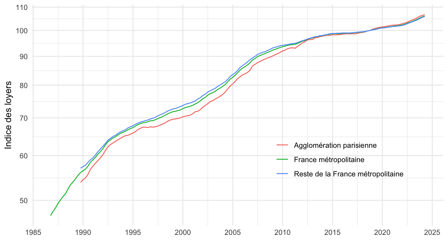
INDICES_LOYERS |>
  bind_rows(IRL) |>
  filter(IDBANK %in% c("001515333", "010600351","010600352", "010600353")) |>
  quarter_to_date() |>
  group_by(date) |>
  filter(n() == 4) |>
  group_by(IDBANK) |>
  arrange(date) |>
  mutate(OBS_VALUE = 100*OBS_VALUE/OBS_VALUE[1]) |>
  mutate(Ref_area = ifelse(IDBANK %in% c("010600351","010600352", "010600353"), paste0("Indice des loyers d'habitation (ILH) - ", Ref_area), "Indice de référence des Loyers (IRL)")) |>
  ggplot() + ylab("Indice des loyers (janvier 2017 = 100)") + xlab("") + theme_minimal() +
  geom_line(aes(x = date, y = OBS_VALUE, color = Ref_area)) +
  scale_x_date(breaks = seq(1920, 2100, 2) |> paste0("-01-01") |> as.Date(),
               labels = date_format("%Y")) +
  theme(legend.position = c(0.4, 0.8),
        legend.title = element_blank()) +
  scale_y_log10(breaks = seq(0, 400, 1),
                     labels = dollar_format(accuracy = 1, prefix = ""))+
  geom_label_repel(data = . %>% filter(date == max(date)),
             aes(x = date, y = OBS_VALUE, color = Ref_area, label = round(OBS_VALUE, 1)),
             show.legend = F)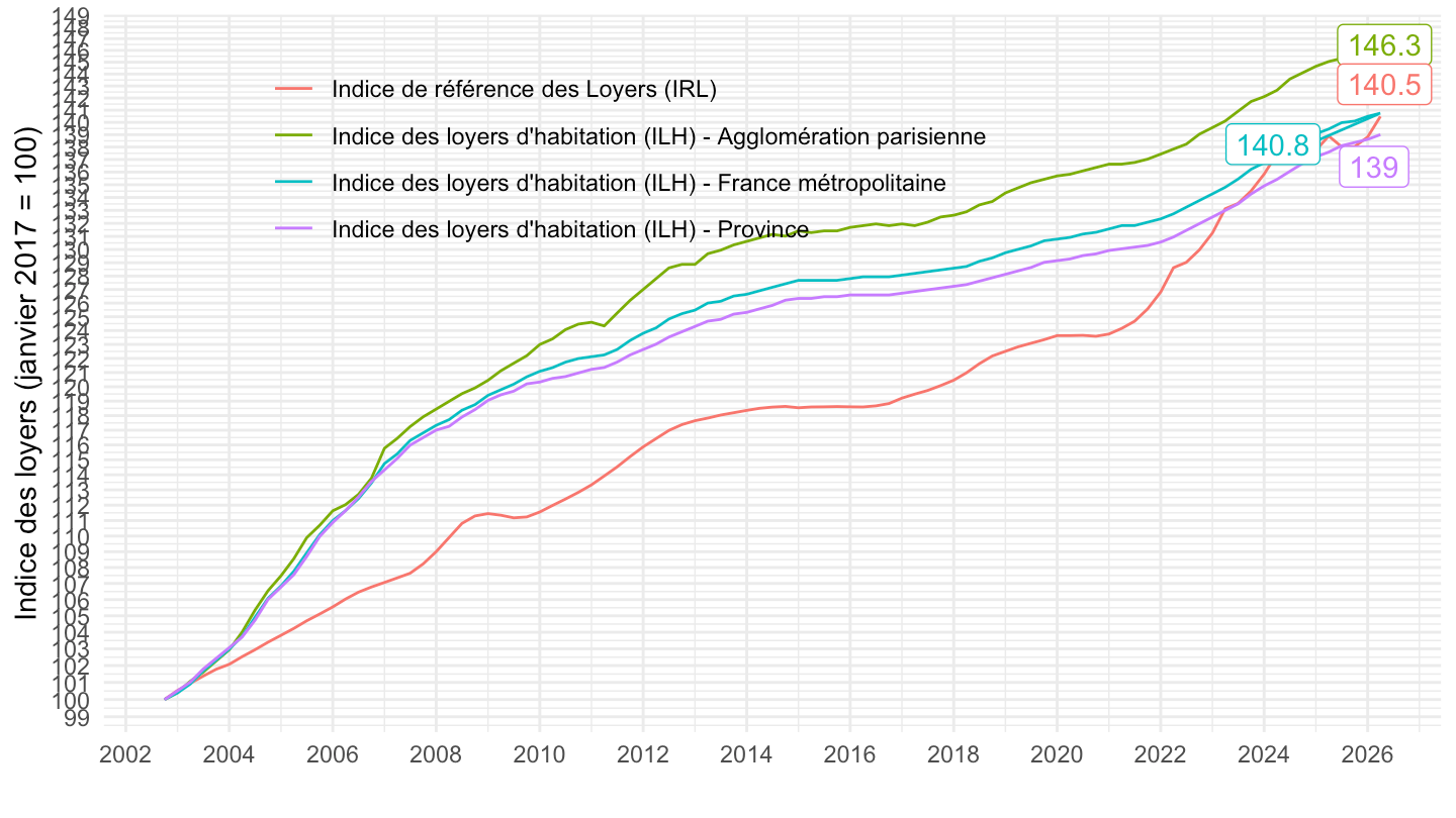
INDICES_LOYERS |>
  bind_rows(IRL) |>
  filter(IDBANK %in% c("001515333", "010600351","010600352", "010600353")) |>
  quarter_to_date() |>
  filter(date >= as.Date("2014-01-01")) |>
  group_by(IDBANK) |>
  arrange(date) |>
  mutate(OBS_VALUE = 100*OBS_VALUE/OBS_VALUE[1]) |>
  mutate(Ref_area = ifelse(IDBANK %in% c("010600351","010600352", "010600353"), paste0("Indice des loyers d'habitation (ILH) - ", Ref_area), "Indice de référence des Loyers (IRL)")) |>
  ggplot() + ylab("Indice des loyers (2014T1 = 100)") + xlab("") + theme_minimal() +
  geom_line(aes(x = date, y = OBS_VALUE, color = Ref_area)) +
  scale_x_date(breaks = seq(1920, 2100, 1) |> paste0("-01-01") |> as.Date(),
               labels = date_format("%Y")) +
  theme(legend.position = c(0.4, 0.8),
        legend.title = element_blank()) +
  scale_y_log10(breaks = seq(0, 400, 1),
                     labels = dollar_format(accuracy = 1, prefix = ""))+
  geom_label_repel(data = . %>% filter(date == max(date)),
             aes(x = date, y = OBS_VALUE, color = Ref_area, label = round(OBS_VALUE, 1)),
             show.legend = F)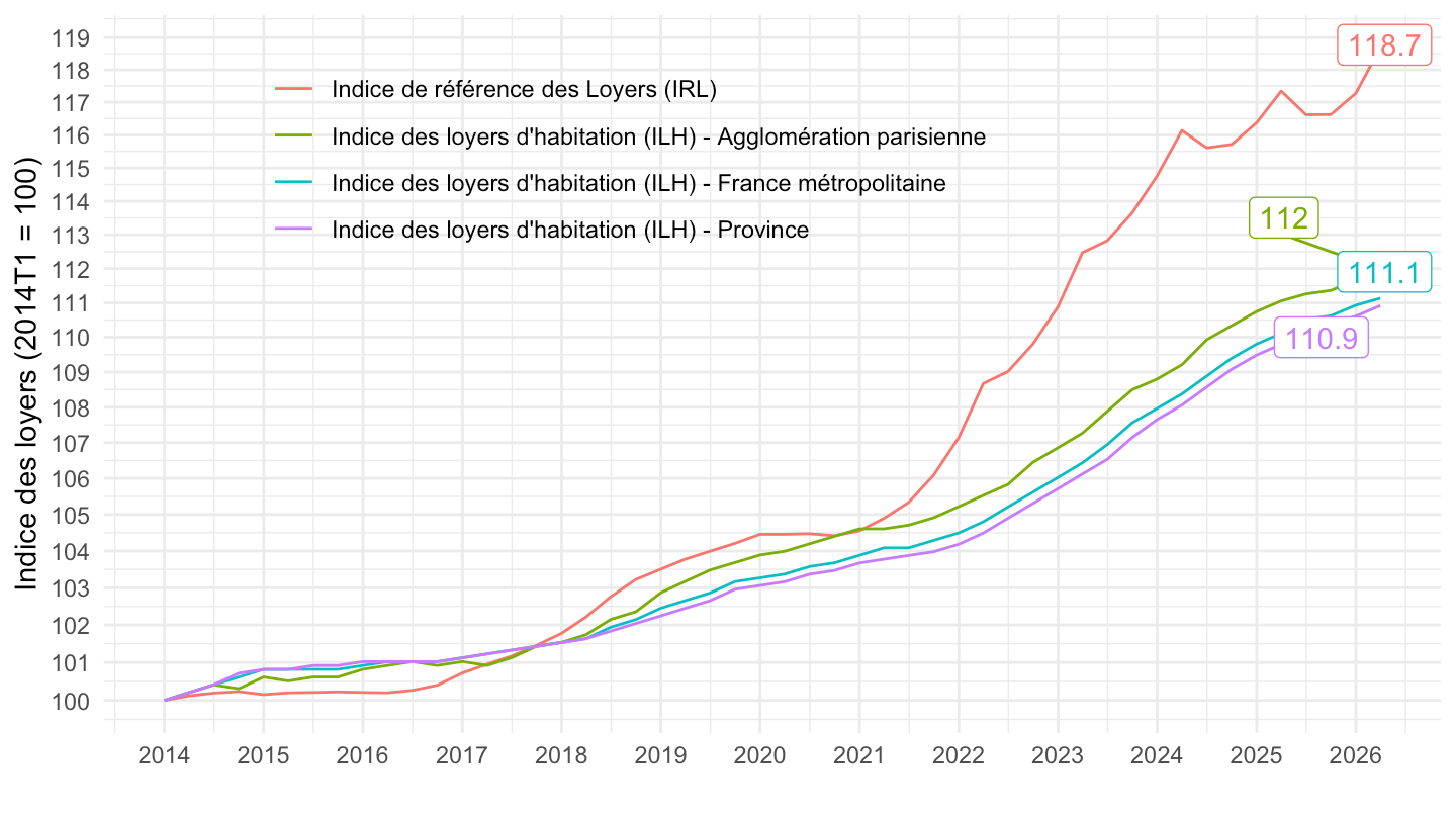
INDICES_LOYERS |>
  bind_rows(IRL) |>
  filter(IDBANK %in% c("001515333", "010600351","010600352", "010600353")) |>
  quarter_to_date() |>
  filter(date >= as.Date("2012-01-01")) |>
  group_by(IDBANK) |>
  arrange(date) |>
  mutate(OBS_VALUE = 100*OBS_VALUE/OBS_VALUE[1]) |>
  mutate(Ref_area = ifelse(IDBANK %in% c("010600351","010600352", "010600353"), paste0("Indice des loyers d'habitation (ILH) - ", Ref_area), "Indice de référence des Loyers (IRL)")) |>
  ggplot() + ylab("Indice des loyers (2014T1 = 100)") + xlab("") + theme_minimal() +
  geom_line(aes(x = date, y = OBS_VALUE, color = Ref_area)) +
  scale_x_date(breaks = seq(1920, 2100, 1) |> paste0("-01-01") |> as.Date(),
               labels = date_format("%Y")) +
  theme(legend.position = c(0.4, 0.8),
        legend.title = element_blank()) +
  scale_y_log10(breaks = seq(0, 400, 1),
                     labels = dollar_format(accuracy = 1, prefix = ""))+
  geom_label_repel(data = . %>% filter(date == max(date)),
             aes(x = date, y = OBS_VALUE, color = Ref_area, label = round(OBS_VALUE, 1)),
             show.legend = F)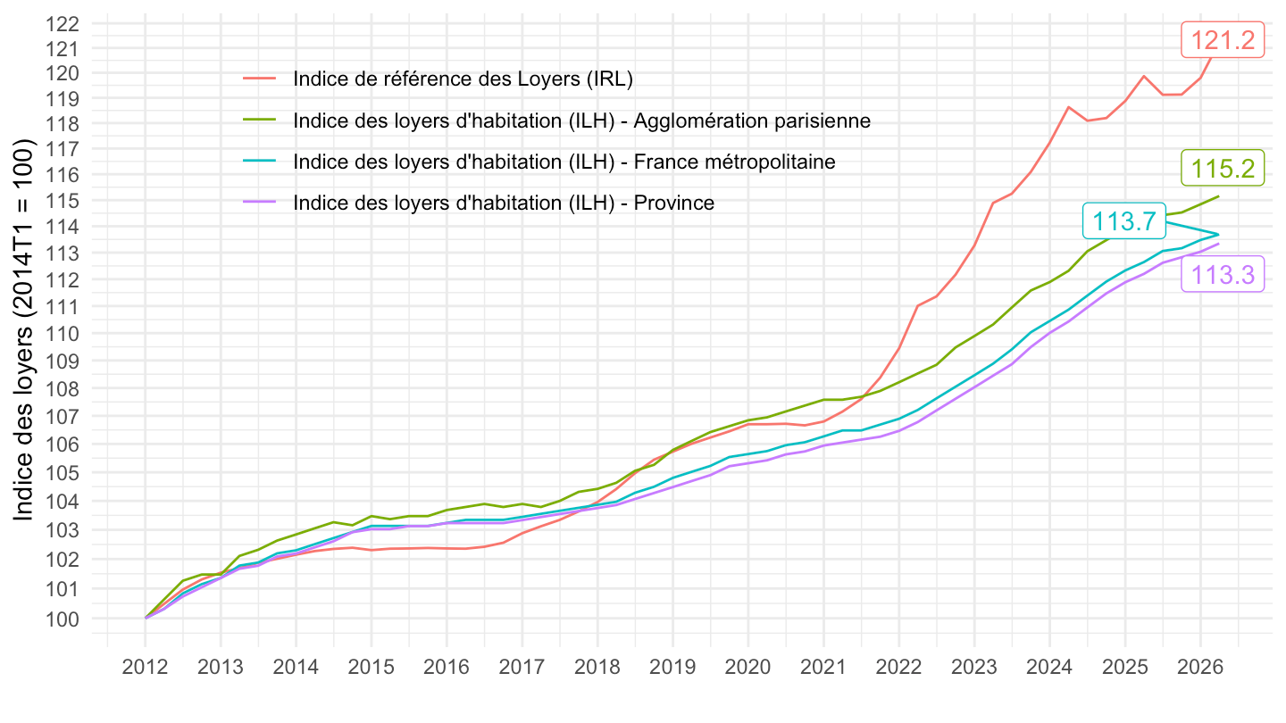
INDICES_LOYERS |>
  filter(SECTEURS_LOYERS == "SECTEUR_LIBRE",
         NATURE == "INDICE",
         REF_AREA %in% c("FM", "AGGLO_PARIS", "PR")) |>
  quarter_to_date() |>
  arrange(desc(date)) |>
  filter(date >= as.Date("2017-01-01")) |>
  group_by(Ref_area) |>
  arrange(date) |>
  mutate(OBS_VALUE = 100*OBS_VALUE/OBS_VALUE[1]) |>
  mutate(Ref_area = paste0("ILH - ", Ref_area)) |>
  ggplot() + ylab("Indice des loyers d'habitation (janvier 2017 = 100)") + xlab("") + theme_minimal() +
  geom_line(aes(x = date, y = OBS_VALUE, color = Ref_area)) +
  scale_x_date(breaks = seq(1920, 2100, 1) |> paste0("-01-01") |> as.Date(),
               labels = date_format("%Y")) +
  theme(legend.position = c(0.3, 0.8),
        legend.title = element_blank()) +
  scale_y_log10(breaks = seq(0, 400, 1),
                     labels = dollar_format(accuracy = 1, prefix = ""))+
  geom_label_repel(data = . %>% filter(date == max(date)),
             aes(x = date, y = OBS_VALUE, color = Ref_area, label = round(OBS_VALUE, 1)),
             show.legend = F)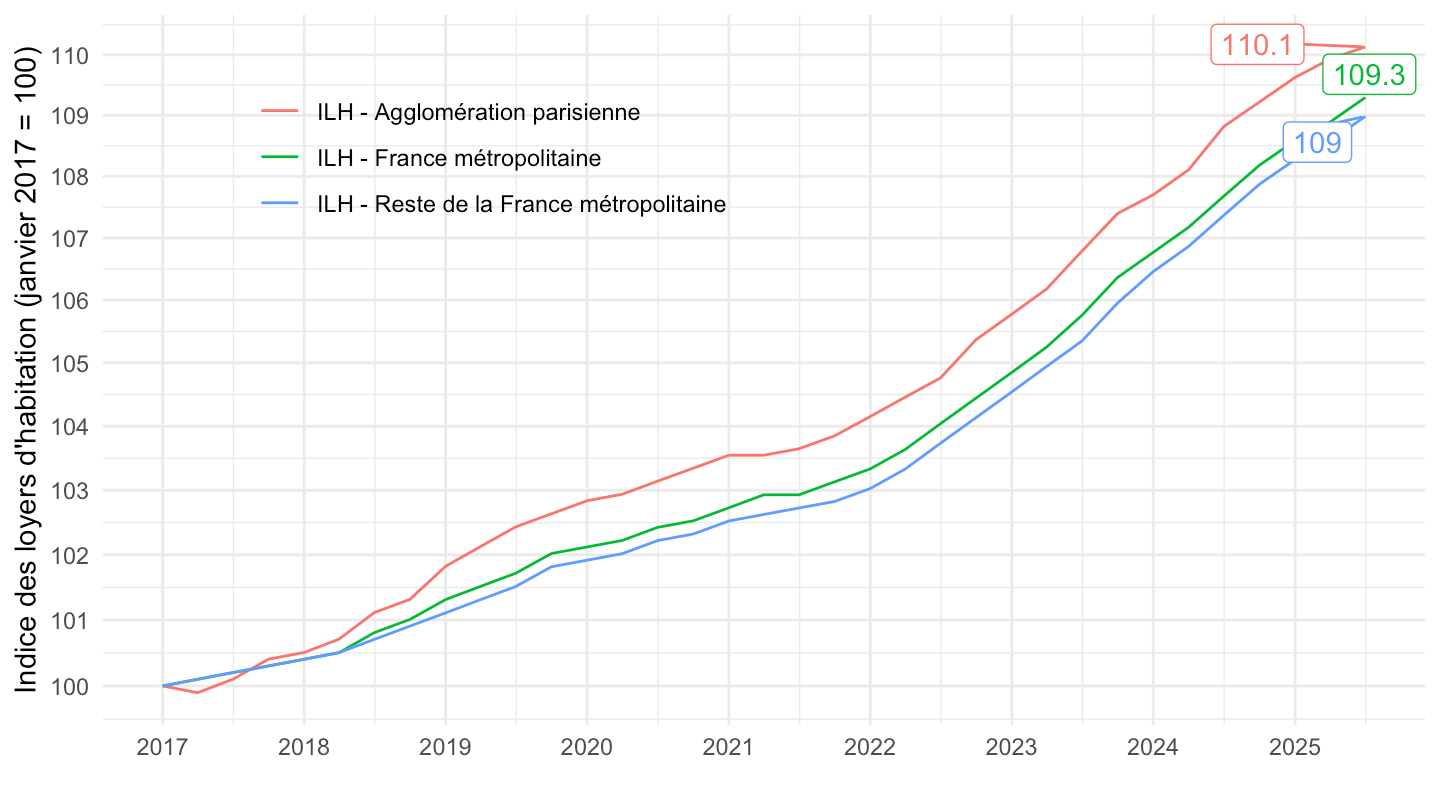
INDICES_LOYERS |>
  bind_rows(IRL) |>
  filter(IDBANK %in% c("001515333", "010600351","010600352", "010600353")) |>
  quarter_to_date() |>
  filter(date >= as.Date("2017-01-01")) |>
  group_by(IDBANK) |>
  arrange(date) |>
  mutate(OBS_VALUE = 100*OBS_VALUE/OBS_VALUE[1]) |>
  mutate(Ref_area = ifelse(IDBANK %in% c("010600351","010600352", "010600353"), paste0("Indice des loyers d'habitation (ILH) - ", Ref_area), "Indice de référence des Loyers (IRL)")) |>
  ggplot() + ylab("Indice des loyers (janvier 2017 = 100)") + xlab("") + theme_minimal() +
  geom_line(aes(x = date, y = OBS_VALUE, color = Ref_area)) +
  scale_x_date(breaks = seq(1920, 2100, 1) |> paste0("-01-01") |> as.Date(),
               labels = date_format("%Y")) +
  theme(legend.position = c(0.4, 0.8),
        legend.title = element_blank()) +
  scale_y_log10(breaks = seq(0, 400, 1),
                     labels = dollar_format(accuracy = 1, prefix = ""))+
  geom_label_repel(data = . %>% filter(date == max(date)),
             aes(x = date, y = OBS_VALUE, color = Ref_area, label = round(OBS_VALUE, 1)),
             show.legend = F)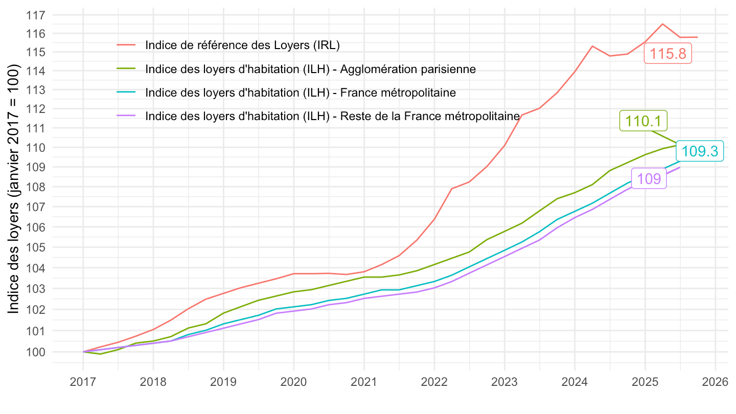
INDICES_LOYERS |>
  bind_rows(IRL) |>
  filter(IDBANK %in% c("010600352")) |>
  quarter_to_date() |>
  filter(date >= as.Date("2001-01-01"),
         date <= as.Date("2025-01-01"),
         month(date) == 1) |>
  select(date, OBS_VALUE) |>
  mutate(variable = "INSEE") |>
  arrange(date) |>
  mutate(OBS_VALUE = 100* OBS_VALUE/OBS_VALUE[1]) |>

  bind_rows(loyers_agglo_paris |>
              mutate(OBS_VALUE = 100*cumprod(1+value/100),
                      year = year+1) |>
              add_row(year = 2001, OBS_VALUE = 100) |>
              mutate(date = paste0(year, "-01-01") |> as.Date()) |>
              mutate(variable = "OLAP")) |>
  bind_rows(`IPCH-IPC-2015-ensemble-Q` |>
              mutate(date = as.Date(date)) |>
              rename(variable = INDICATEUR) |>
              group_by(variable) |>
              filter(date >= as.Date("2001-01-01"),
                     date <= as.Date("2025-01-01")) |>
              arrange(date) |>
              mutate(OBS_VALUE = 100* OBS_VALUE/OBS_VALUE[1])) |>
  mutate(variable = factor(variable,
                           levels = c("OLAP",
                                      "IPCH",
                                      "INSEE",
                                      "IPC"),
                           labels = c("Indice des Loyers de l'Agglomération Parisienne. Source: OLAP",
                                      "Indice des Prix à la Consommation Harmonisé (IPCH) - Eurostat",
                                      "Indice des Loyers de l'Agglomération Parisienne. Source: INSEE",
                                      "Indice des Prix à la Consommation (IPC) - Insee"))) |>
  ggplot() + ylab("Janvier 2001 = 100") + xlab("") + theme_minimal() +
  geom_line(aes(x = date, y = OBS_VALUE, color = variable)) +
  scale_x_date(breaks = seq(1920, 2100, 2) |> paste0("-01-01") |> as.Date(),
               labels = date_format("%Y")) +
  theme(legend.position = c(0.4, 0.9),
        legend.title = element_blank()) +
  scale_y_log10(breaks = seq(0, 400, 5),
                     labels = dollar_format(accuracy = 1, prefix = ""))+
  geom_label_repel(data = . %>% filter(date == max(date)),
             aes(x = date, y = OBS_VALUE, color = variable, label = round(OBS_VALUE, 1)),
             show.legend = F)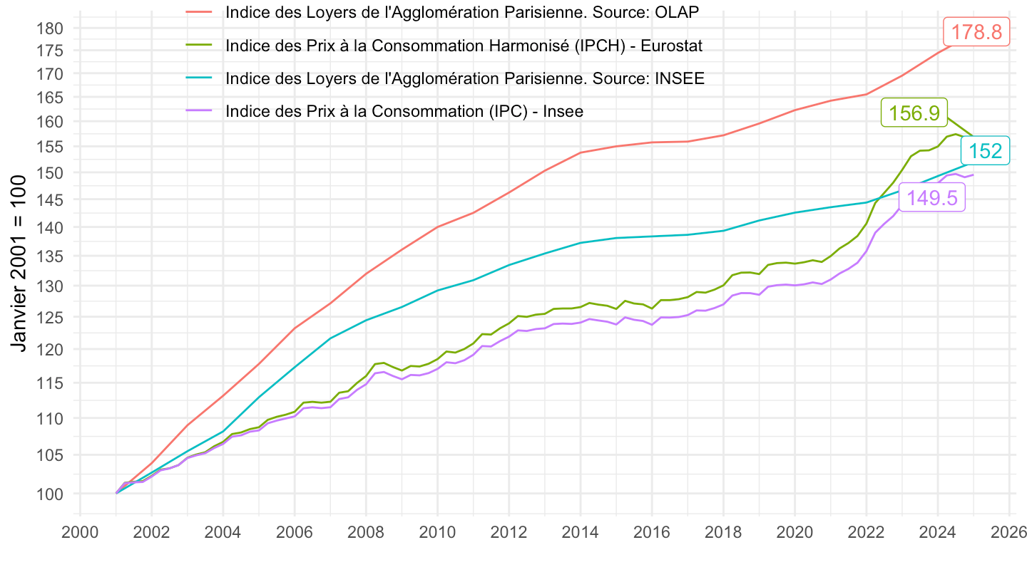
INDICES_LOYERS |>
  bind_rows(IRL) |>
  filter(IDBANK %in% c("010600352")) |>
  quarter_to_date() |>
  filter(date >= as.Date("2017-01-01"),
         date <= as.Date("2025-01-01"),
         month(date) == 1) |>
  select(date, OBS_VALUE) |>
  mutate(variable = "INSEE") |>
  arrange(date) |>
  mutate(OBS_VALUE = 100* OBS_VALUE/OBS_VALUE[1]) |>

  bind_rows(loyers_agglo_paris |>
              filter(year >=2017) |>
              mutate(OBS_VALUE = 100*cumprod(1+value/100),
                      year = year+1) |>
              add_row(year = 2017, OBS_VALUE = 100) |>
              mutate(date = paste0(year, "-01-01") |> as.Date()) |>
              mutate(variable = "OLAP")) |>
  mutate(variable = factor(variable,
                           levels = c("OLAP",
                                      "INSEE"),
                           labels = c("Indice des Loyers de l'Agglomération Parisienne. Source: OLAP",
                                      "Indice des Loyers de l'Agglomération Parisienne. Source: INSEE"))) |>
  ggplot() + ylab("Indice des loyers (janvier 2017 = 100)") + xlab("") + theme_minimal() +
  geom_line(aes(x = date, y = OBS_VALUE, color = variable)) +
  scale_x_date(breaks = seq(1920, 2100, 1) |> paste0("-01-01") |> as.Date(),
               labels = date_format("%Y")) +
  theme(legend.position = c(0.4, 0.9),
        legend.title = element_blank()) +
  scale_y_log10(breaks = seq(0, 400, 2),
                     labels = dollar_format(accuracy = 1, prefix = ""))+
  geom_label(data = . %>% filter(date == max(date)),
             aes(x = date, y = OBS_VALUE, color = variable, label = round(OBS_VALUE, 1)),
             show.legend = F)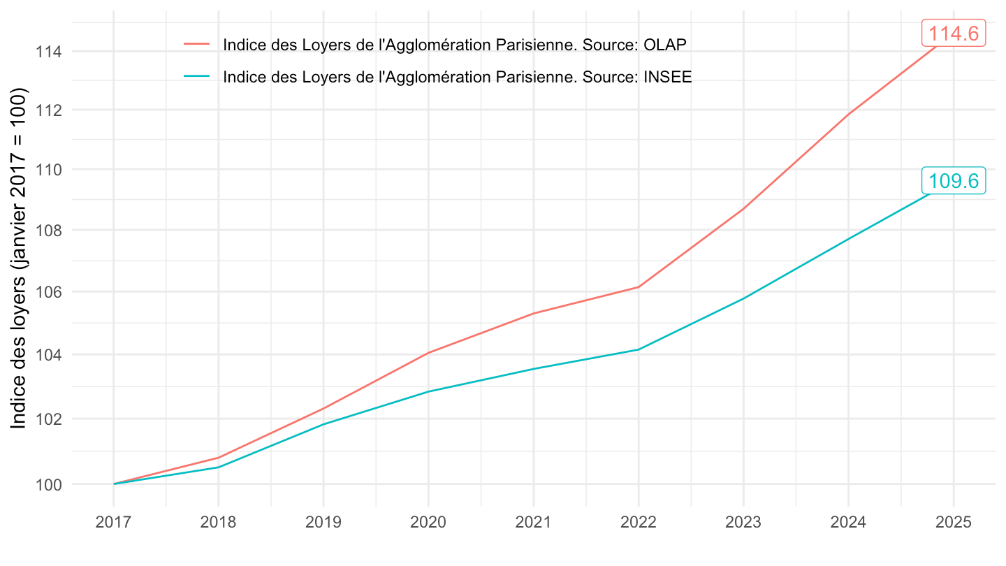
INDICES_LOYERS |>
  bind_rows(IRL) |>
  filter(IDBANK %in% c("001515333", "010600351","010600352", "010600353")) |>
  quarter_to_date() |>
  filter(date >= as.Date("2001-01-01"),
         date <= as.Date("2025-01-01")) |>
  group_by(IDBANK) |>
  arrange(date) |>
  mutate(OBS_VALUE = 100*OBS_VALUE/OBS_VALUE[1]) |>
  mutate(Ref_area = ifelse(IDBANK %in% c("010600351","010600352", "010600353"), paste0("Indice des loyers d'habitation (ILH) - ", Ref_area), "Indice de référence des Loyers (IRL)")) |>
  ggplot() + ylab("Indice des loyers (janvier 2017 = 100)") + xlab("") + theme_minimal() +
  geom_line(aes(x = date, y = OBS_VALUE, color = Ref_area)) +
  scale_x_date(breaks = seq(1920, 2100, 2) |> paste0("-01-01") |> as.Date(),
               labels = date_format("%Y")) +
  theme(legend.position = c(0.4, 0.8),
        legend.title = element_blank()) +
  scale_y_log10(breaks = seq(0, 400, 5),
                     labels = dollar_format(accuracy = 1, prefix = ""))+
  geom_label_repel(data = . %>% filter(date == max(date)),
             aes(x = date, y = OBS_VALUE, color = Ref_area, label = round(OBS_VALUE, 1)),
             show.legend = F)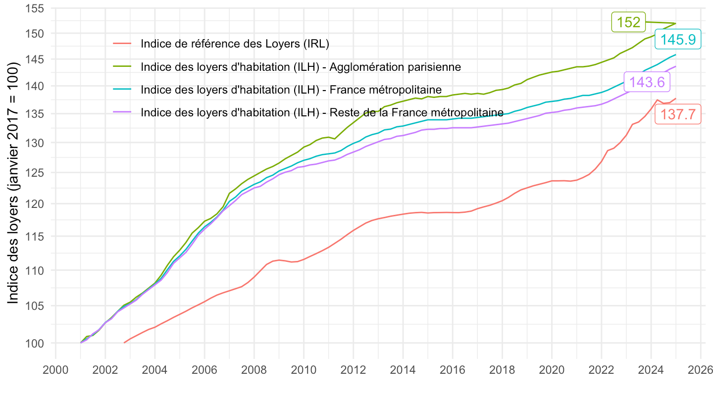
INDICES_LOYERS |>
  bind_rows(IRL) |>
  filter(IDBANK %in% c("010600352")) |>
  quarter_to_date() |>
  filter(date >= as.Date("2001-01-01"),
         date <= as.Date("2021-01-01"),
         month(date) == 1) |>
  select(date, OBS_VALUE) |>
  mutate(variable = "INSEE") |>
  arrange(date) |>
  mutate(OBS_VALUE = 100* OBS_VALUE/OBS_VALUE[1]) |>

  bind_rows(loyers_agglo_paris |>
              mutate(OBS_VALUE = 100*cumprod(1+value/100),
                      year = year+1) |>
              add_row(year = 2001, OBS_VALUE = 100) |>
              mutate(date = paste0(year, "-01-01") |> as.Date()) |>
              mutate(variable = "OLAP") |>
              filter(date <= as.Date("2021-01-01"))) |>
  bind_rows(`IPCH-IPC-2015-ensemble-Q` |>
              mutate(date = as.Date(date)) |>
              rename(variable = INDICATEUR) |>
              group_by(variable) |>
              filter(date >= as.Date("2001-01-01"),
                     date <= as.Date("2021-01-01")) |>
              arrange(date) |>
              mutate(OBS_VALUE = 100* OBS_VALUE/OBS_VALUE[1])) |>
  mutate(variable = factor(variable,
                           levels = c("OLAP",
                                      "INSEE",
                                      "IPCH",
                                      "IPC"),
                           labels = c("Indice des Loyers de l'Agglomération Parisienne. Source: OLAP",
                                      "Indice des Loyers de l'Agglomération Parisienne. Source: INSEE",
                                      "Indice des Prix à la Consommation Harmonisé (IPCH) - Eurostat",
                                      "Indice des Prix à la Consommation (IPC) - Insee"))) |>
  ggplot() + ylab("Janvier 2001 = 100") + xlab("") + theme_minimal() +
  geom_line(aes(x = date, y = OBS_VALUE, color = variable)) +
  scale_x_date(breaks = seq(2001, 2100, 2) |> paste0("-01-01") |> as.Date(),
               labels = date_format("%Y")) +
  theme(legend.position = c(0.32, 0.85),
        legend.title = element_blank()) +
  scale_y_log10(breaks = seq(0, 400, 5),
                     labels = dollar_format(accuracy = 1, prefix = ""))+
  geom_label(data = . %>% filter(date == max(date)),
             aes(x = date, y = OBS_VALUE, color = variable, label = round(OBS_VALUE, 1)),
             show.legend = F)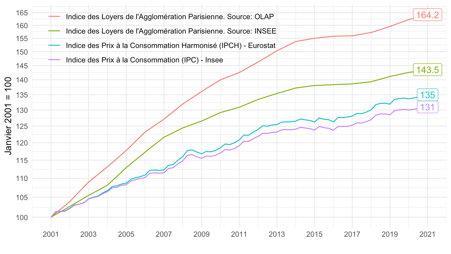
INDICES_LOYERS |>
  bind_rows(IRL) |>
  filter(IDBANK %in% c("010600352")) |>
  quarter_to_date() |>
  filter(date >= as.Date("2001-01-01"),
         date <= as.Date("2024-01-01"),
         month(date) == 1) |>
  select(date, OBS_VALUE) |>
  mutate(variable = "INSEE") |>
  arrange(date) |>
  mutate(OBS_VALUE = 100* OBS_VALUE/OBS_VALUE[1]) |>

  bind_rows(loyers_agglo_paris |>
              mutate(OBS_VALUE = 100*cumprod(1+value/100),
                      year = year+1) |>
              add_row(year = 2001, OBS_VALUE = 100) |>
              mutate(date = paste0(year, "-01-01") |> as.Date()) |>
              mutate(variable = "OLAP") |>
              filter(date <= as.Date("2024-01-01"))) |>
  bind_rows(`IPCH-IPC-2015-ensemble-Q` |>
              mutate(date = as.Date(date)) |>
              rename(variable = INDICATEUR) |>
              group_by(variable) |>
              filter(date >= as.Date("2001-01-01"),
                     date <= as.Date("2024-01-01")) |>
              arrange(date) |>
              mutate(OBS_VALUE = 100* OBS_VALUE/OBS_VALUE[1])) |>
  mutate(variable = factor(variable,
                           levels = c("OLAP",
                                      "IPCH",
                                      "INSEE",
                                      "IPC"),
                           labels = c("Indice des Loyers de l'Agglomération Parisienne. Source: OLAP",
                                      "Indice des Prix à la Consommation Harmonisé (IPCH) - Eurostat",
                                      "Indice des Loyers de l'Agglomération Parisienne. Source: INSEE",
                                      "Indice des Prix à la Consommation (IPC) - Insee"))) |>
  ggplot() + ylab("Janvier 2001 = 100") + xlab("") + theme_minimal() +
  geom_line(aes(x = date, y = OBS_VALUE, color = variable)) +
  scale_x_date(breaks = seq(2001, 2100, 2) |> paste0("-01-01") |> as.Date(),
               labels = date_format("%Y")) +
  theme(legend.position = c(0.35, 0.85),
        legend.title = element_blank()) +
  scale_y_log10(breaks = seq(0, 400, 5),
                     labels = dollar_format(accuracy = 1, prefix = ""))+
  geom_label_repel(data = . %>% filter(date == max(date)),
             aes(x = date, y = OBS_VALUE, color = variable, label = round(OBS_VALUE, 1)),
             show.legend = F)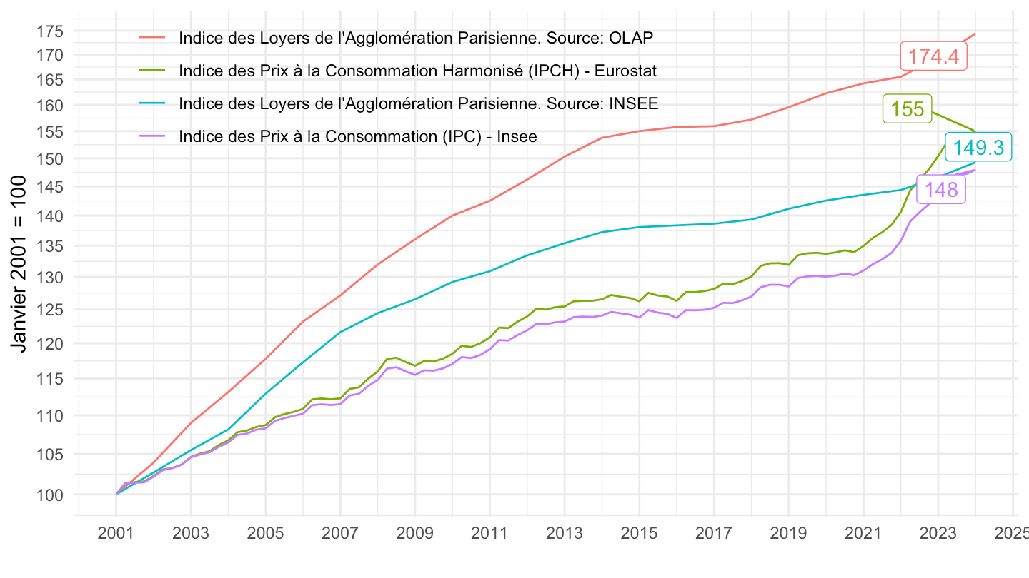
INDICES_LOYERS |>
  bind_rows(IRL) |>
  filter(IDBANK %in% c("001515333", "010600351","010600352", "010600353")) |>
  quarter_to_date() |>
  filter(date >= as.Date("2017-01-01"),
         date <= as.Date("2025-01-01")) |>
  group_by(IDBANK) |>
  arrange(date) |>
  mutate(OBS_VALUE = 100*OBS_VALUE/OBS_VALUE[1]) |>
  mutate(Ref_area = ifelse(IDBANK %in% c("010600351","010600352", "010600353"), paste0("Indice des loyers d'habitation (ILH) - ", Ref_area), "Indice de référence des Loyers (IRL)")) |>
  ggplot() + ylab("Indice des loyers (janvier 2017 = 100)") + xlab("") + theme_minimal() +
  geom_line(aes(x = date, y = OBS_VALUE, color = Ref_area)) +
  scale_x_date(breaks = seq(1920, 2100, 1) |> paste0("-01-01") |> as.Date(),
               labels = date_format("%Y")) +
  theme(legend.position = c(0.4, 0.8),
        legend.title = element_blank()) +
  scale_y_log10(breaks = seq(0, 400, 1),
                     labels = dollar_format(accuracy = 1, prefix = ""))+
  geom_label_repel(data = . %>% filter(date == max(date)),
             aes(x = date, y = OBS_VALUE, color = Ref_area, label = round(OBS_VALUE, 1)),
             show.legend = F)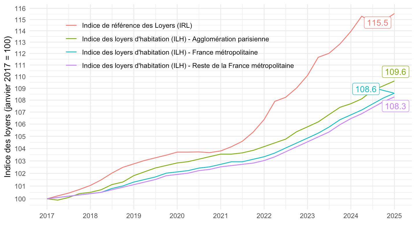
INDICES_LOYERS |>
  bind_rows(IRL) |>
  filter(IDBANK %in% c("001515333", "010600351","010600352", "010600353")) |>
  quarter_to_date() |>
  filter(date >= as.Date("2017-01-01"),
         date <= as.Date("2024-01-01")) |>
  group_by(IDBANK) |>
  arrange(date) |>
  mutate(OBS_VALUE = 100*OBS_VALUE/OBS_VALUE[1]) |>
  mutate(Ref_area = ifelse(IDBANK %in% c("010600351","010600352", "010600353"), paste0("Indice des loyers d'habitation (ILH) - ", Ref_area), "Indice de référence des Loyers (IRL)")) |>
  ggplot() + ylab("Indice des loyers (janvier 2017 = 100)") + xlab("") + theme_minimal() +
  geom_line(aes(x = date, y = OBS_VALUE, color = Ref_area)) +
  scale_x_date(breaks = seq(1920, 2100, 1) |> paste0("-01-01") |> as.Date(),
               labels = date_format("%Y")) +
  theme(legend.position = c(0.4, 0.8),
        legend.title = element_blank()) +
  scale_y_log10(breaks = seq(0, 400, 1),
                     labels = dollar_format(accuracy = 1, prefix = ""))+
  geom_label_repel(data = . %>% filter(date == max(date)),
             aes(x = date, y = OBS_VALUE, color = Ref_area, label = round(OBS_VALUE, 1)),
             show.legend = F)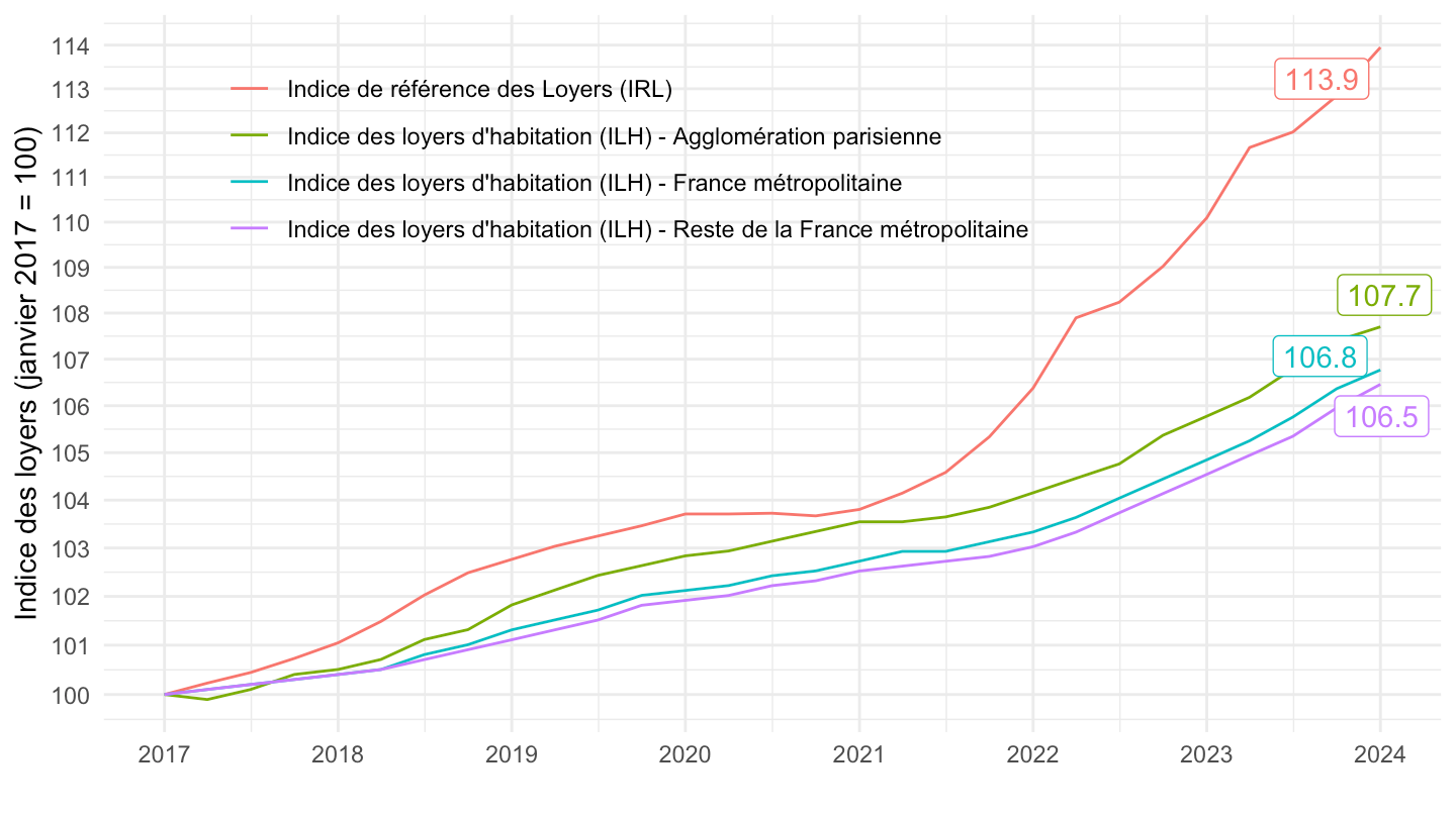
INDICES_LOYERS |>
  filter(SECTEURS_LOYERS == "SECTEUR_SOCIAL",
         NATURE == "INDICE",
         REF_AREA %in% c("FM", "AGGLO_PARIS", "PR")) |>
  quarter_to_date() |>
  ggplot() + ylab("Indice des loyers") + xlab("") + theme_minimal() +
  geom_line(aes(x = date, y = OBS_VALUE, color = Ref_area)) +

  scale_x_date(breaks = seq(1920, 2100, 5) |> paste0("-01-01") |> as.Date(),
               labels = date_format("%Y")) +
  theme(legend.position = c(0.75, 0.3),
        legend.title = element_blank()) +
  scale_y_log10(breaks = seq(0, 400, 10),
                     labels = dollar_format(accuracy = 1, prefix = ""))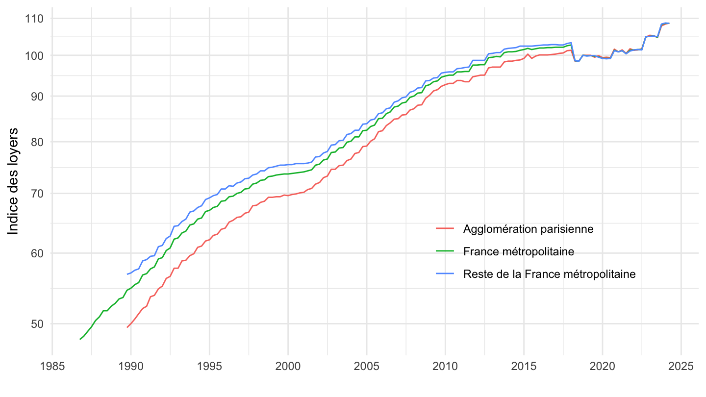
INDICES_LOYERS |>
  filter(TIME_PERIOD == "2020-Q2",
         NATURE == "INDICE",
         SECTEURS_LOYERS == "TOUS_SECTEURS") |>
  select(REF_AREA, TITLE_FR, OBS_VALUE) |>
  mutate(TITLE_FR = gsub("Indice des loyers – Tous secteurs – ", "", TITLE_FR),
         TITLE_FR = gsub(" – Base 100 en janvier 2019", "", TITLE_FR)) %>%
{if (is_html_output()) print_table(.) else .}| REF_AREA | TITLE_FR | OBS_VALUE |
|---|---|---|
| FM | France métropolitaine | 100.6 |
| AGGLO_PARIS | Agglomération parisienne | 100.8 |
| PR | Reste de la France métropolitaine | 100.5 |
| D971 | Guadeloupe | 101.1 |
| D972 | Martinique | 101.2 |
| D973 | Guyane | 101.0 |
| D974 | La Réunion | 101.1 |
| FR-D976 | France (hors Mayotte) | 100.6 |
INDICES_LOYERS |>
  filter(REF_AREA == "FM",
         NATURE == "INDICE") |>
  quarter_to_date() |>
  ggplot() + ylab("Indice des loyers") + xlab("") + theme_minimal() +
  geom_line(aes(x = date, y = OBS_VALUE, color = Secteurs_loyers)) +

  scale_x_date(breaks = seq(1920, 2100, 5) |> paste0("-01-01") |> as.Date(),
               labels = date_format("%Y")) +
  theme(legend.position = c(0.75, 0.3),
        legend.title = element_blank()) +
  scale_y_log10(breaks = seq(0, 400, 10),
                     labels = dollar_format(accuracy = 1, prefix = ""))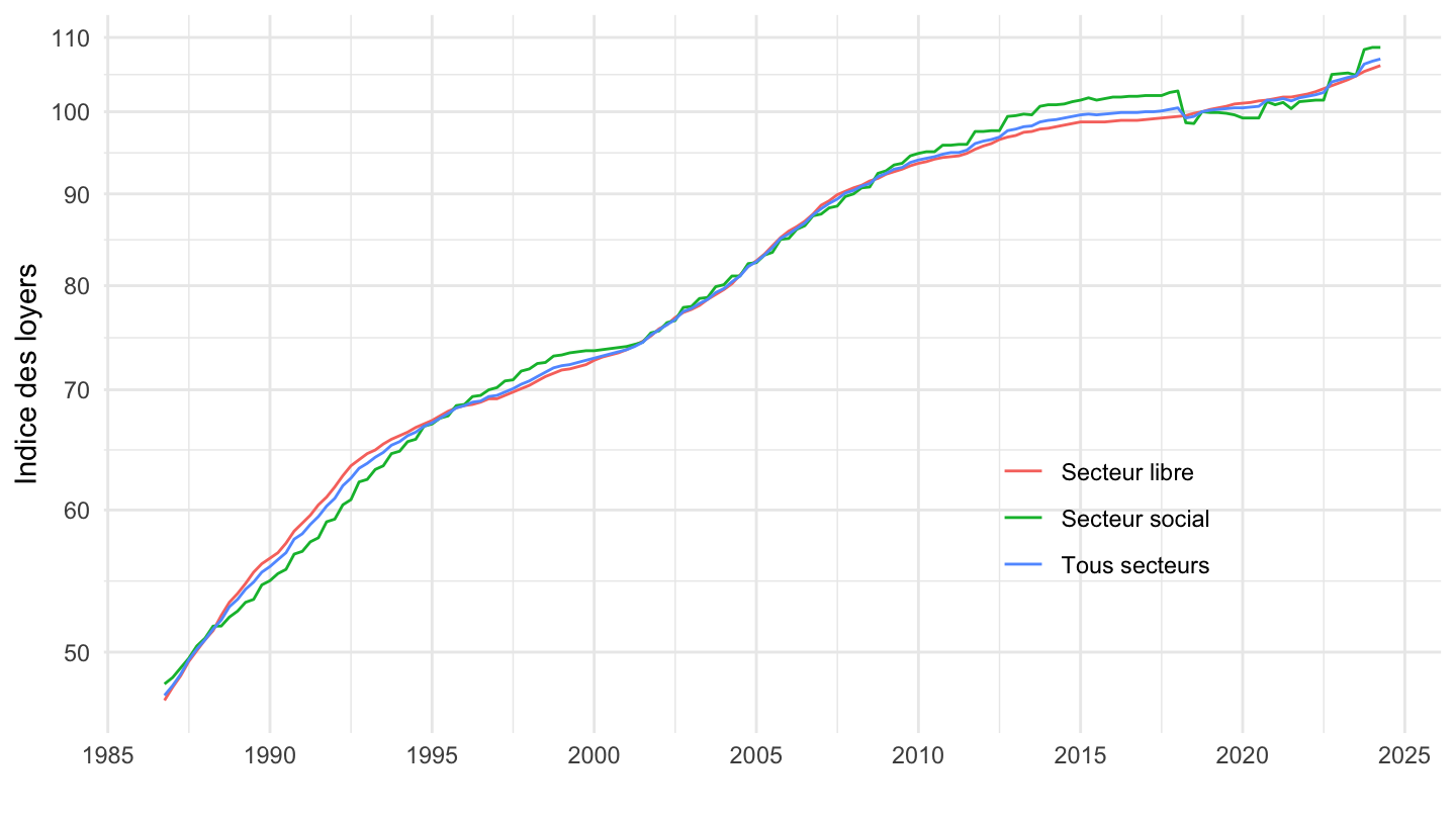
INDICES_LOYERS |>
  filter(REF_AREA == "FM",
         NATURE == "INDICE") |>
  quarter_to_date() |>
  filter(date >= as.Date("1990-01-01")) |>
  group_by(SECTEURS_LOYERS) |>
  arrange(date) |>
  mutate(OBS_VALUE = 100*OBS_VALUE/OBS_VALUE[1]) |>
  ggplot() + ylab("Indice des loyers") + xlab("") + theme_minimal() +
  geom_line(aes(x = date, y = OBS_VALUE, color = Secteurs_loyers)) +

  scale_x_date(breaks = seq(1920, 2100, 5) |> paste0("-01-01") |> as.Date(),
               labels = date_format("%Y")) +
  theme(legend.position = c(0.75, 0.3),
        legend.title = element_blank()) +
  scale_y_log10(breaks = seq(0, 400, 10),
                     labels = dollar_format(accuracy = 1, prefix = ""))
INDICES_LOYERS |>
  filter(REF_AREA == "FM",
         NATURE == "INDICE") |>
  quarter_to_date() |>
  filter(date >= as.Date("1992-01-01")) |>
  group_by(SECTEURS_LOYERS) |>
  arrange(date) |>
  mutate(OBS_VALUE = 100*OBS_VALUE/OBS_VALUE[1]) |>
  ggplot() + ylab("Indice des loyers") + xlab("") + theme_minimal() +
  geom_line(aes(x = date, y = OBS_VALUE, color = Secteurs_loyers)) +

  scale_x_date(breaks = seq(1920, 2100, 2) |> paste0("-01-01") |> as.Date(),
               labels = date_format("%Y")) +
  theme(legend.position = c(0.75, 0.3),
        legend.title = element_blank()) +
  scale_y_log10(breaks = seq(0, 400, 10),
                     labels = dollar_format(accuracy = 1, prefix = ""))
INDICES_LOYERS |>
  filter(REF_AREA == "FM",
         NATURE == "INDICE") |>
  quarter_to_date() |>
  filter(date >= as.Date("2000-01-01")) |>
  group_by(SECTEURS_LOYERS) |>
  arrange(date) |>
  mutate(OBS_VALUE = 100*OBS_VALUE/OBS_VALUE[1]) |>
  ggplot() + ylab("Indice des loyers") + xlab("") + theme_minimal() +
  geom_line(aes(x = date, y = OBS_VALUE, color = Secteurs_loyers)) +

  scale_x_date(breaks = seq(1920, 2100, 5) |> paste0("-01-01") |> as.Date(),
               labels = date_format("%Y")) +
  theme(legend.position = c(0.75, 0.3),
        legend.title = element_blank()) +
  scale_y_log10(breaks = seq(0, 400, 10),
                     labels = dollar_format(accuracy = 1, prefix = ""))
INDICES_LOYERS |>
  filter(REF_AREA == "FM",
         NATURE == "INDICE") |>
  quarter_to_date() |>
  filter(date >= as.Date("2017-01-01")) |>
  group_by(SECTEURS_LOYERS) |>
  arrange(date) |>
  mutate(OBS_VALUE = 100*OBS_VALUE/OBS_VALUE[1]) |>
  ggplot() + ylab("Indice des loyers") + xlab("") + theme_minimal() +
  geom_line(aes(x = date, y = OBS_VALUE, color = Secteurs_loyers)) +

  scale_x_date(breaks = seq(1920, 2100, 1) |> paste0("-01-01") |> as.Date(),
               labels = date_format("%Y")) +
  theme(legend.position = c(0.75, 0.3),
        legend.title = element_blank()) +
  scale_y_log10(breaks = seq(0, 400, 1),
                     labels = dollar_format(accuracy = 1, prefix = "")) +
  geom_label(data = . %>% filter(date == max(date)),
             aes(x = date, y = OBS_VALUE, color = Secteurs_loyers, label = round(OBS_VALUE, 1)),
             show.legend = F)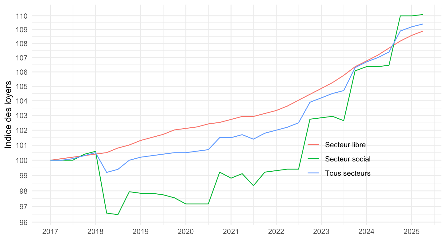
INDICES_LOYERS |>
  filter(REF_AREA == "AGGLO_PARIS",
         NATURE == "INDICE") |>
  quarter_to_date() |>
  ggplot() + ylab("Indice des loyers") + xlab("") + theme_minimal() +
  geom_line(aes(x = date, y = OBS_VALUE, color = Secteurs_loyers)) +

  scale_x_date(breaks = seq(1920, 2100, 5) |> paste0("-01-01") |> as.Date(),
               labels = date_format("%Y")) +
  theme(legend.position = c(0.75, 0.3),
        legend.title = element_blank()) +
  scale_y_log10(breaks = seq(0, 400, 10),
                     labels = dollar_format(accuracy = 1, prefix = ""))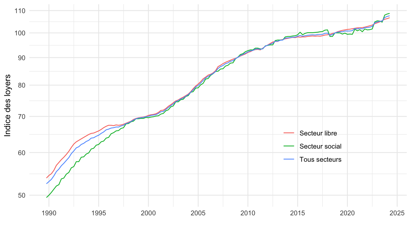
INDICES_LOYERS |>
  filter(REF_AREA == "AGGLO_PARIS",
         NATURE == "INDICE") |>
  quarter_to_date() |>
  filter(date >= as.Date("1990-01-01")) |>
  group_by(SECTEURS_LOYERS) |>
  arrange(date) |>
  mutate(OBS_VALUE = 100*OBS_VALUE/OBS_VALUE[1]) |>
  ggplot() + ylab("Indice des loyers") + xlab("") + theme_minimal() +
  geom_line(aes(x = date, y = OBS_VALUE, color = Secteurs_loyers)) +

  scale_x_date(breaks = seq(1920, 2100, 5) |> paste0("-01-01") |> as.Date(),
               labels = date_format("%Y")) +
  theme(legend.position = c(0.75, 0.3),
        legend.title = element_blank()) +
  scale_y_log10(breaks = seq(0, 400, 10),
                     labels = dollar_format(accuracy = 1, prefix = ""))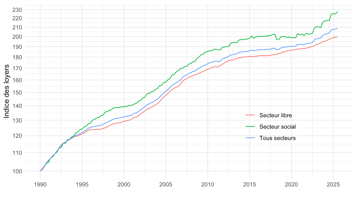
INDICES_LOYERS |>
  filter(REF_AREA == "AGGLO_PARIS",
         NATURE == "INDICE") |>
  quarter_to_date() |>
  filter(date >= as.Date("1992-01-01")) |>
  group_by(SECTEURS_LOYERS) |>
  arrange(date) |>
  mutate(OBS_VALUE = 100*OBS_VALUE/OBS_VALUE[1]) |>
  ggplot() + ylab("Indice des loyers") + xlab("") + theme_minimal() +
  geom_line(aes(x = date, y = OBS_VALUE, color = Secteurs_loyers)) +

  scale_x_date(breaks = seq(1920, 2100, 2) |> paste0("-01-01") |> as.Date(),
               labels = date_format("%Y")) +
  theme(legend.position = c(0.75, 0.3),
        legend.title = element_blank()) +
  scale_y_log10(breaks = seq(0, 400, 10),
                     labels = dollar_format(accuracy = 1, prefix = ""))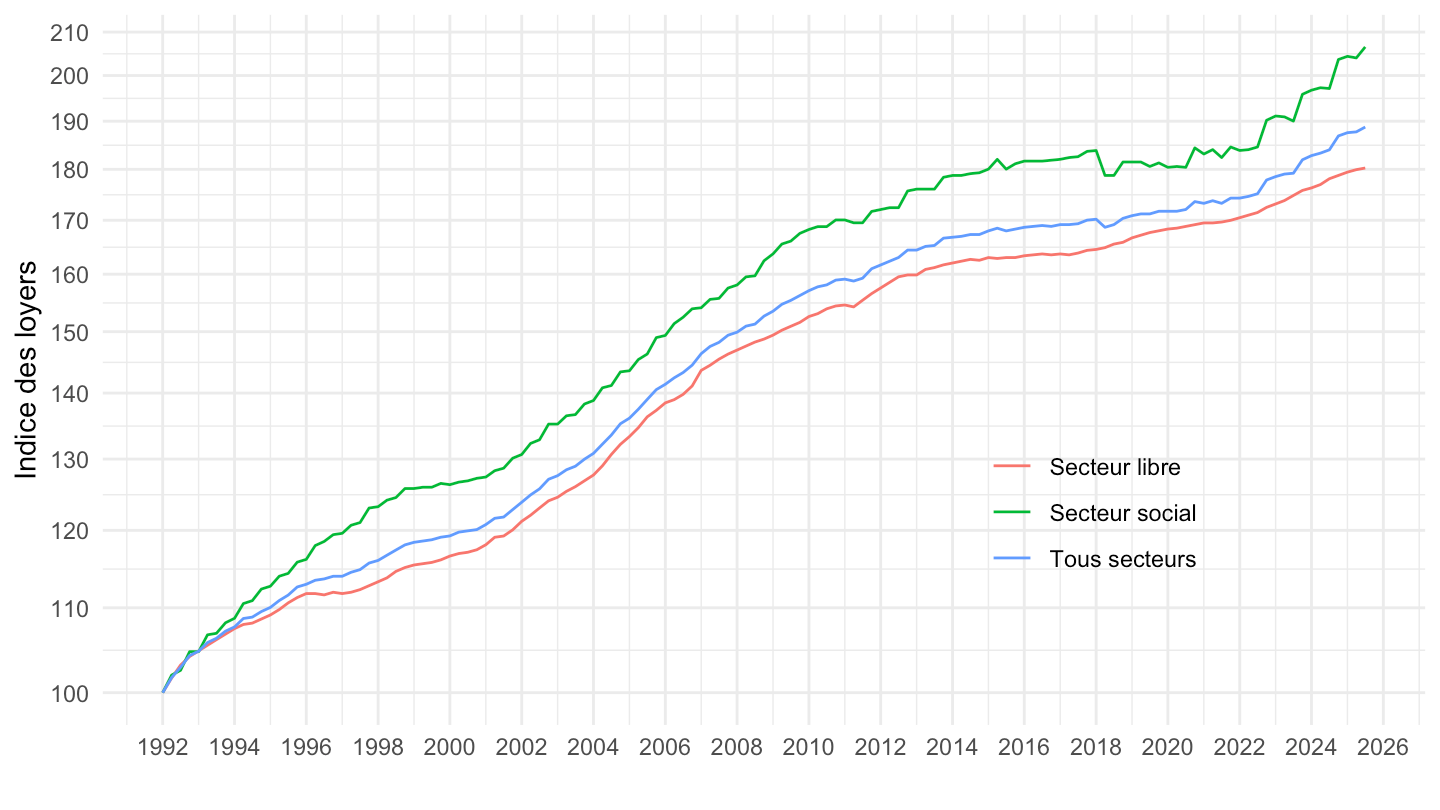
INDICES_LOYERS |>
  filter(REF_AREA == "AGGLO_PARIS",
         NATURE == "INDICE") |>
  quarter_to_date() |>
  filter(date >= as.Date("2000-01-01")) |>
  group_by(SECTEURS_LOYERS) |>
  arrange(date) |>
  mutate(OBS_VALUE = 100*OBS_VALUE/OBS_VALUE[1]) |>
  ggplot() + ylab("Indice des loyers") + xlab("") + theme_minimal() +
  geom_line(aes(x = date, y = OBS_VALUE, color = Secteurs_loyers)) +

  scale_x_date(breaks = seq(1920, 2100, 5) |> paste0("-01-01") |> as.Date(),
               labels = date_format("%Y")) +
  theme(legend.position = c(0.75, 0.3),
        legend.title = element_blank()) +
  scale_y_log10(breaks = seq(0, 400, 10),
                     labels = dollar_format(accuracy = 1, prefix = ""))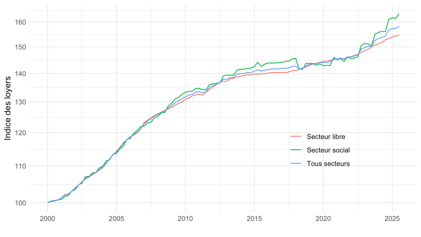
INDICES_LOYERS |>
  filter(REF_AREA == "AGGLO_PARIS",
         NATURE == "INDICE") |>
  quarter_to_date() |>
  filter(date >= as.Date("2017-01-01")) |>
  group_by(SECTEURS_LOYERS) |>
  arrange(date) |>
  mutate(OBS_VALUE = 100*OBS_VALUE/OBS_VALUE[1]) |>
  ggplot() + ylab("Indice des loyers") + xlab("") + theme_minimal() +
  geom_line(aes(x = date, y = OBS_VALUE, color = Secteurs_loyers)) +

  scale_x_date(breaks = seq(1920, 2100, 1) |> paste0("-01-01") |> as.Date(),
               labels = date_format("%Y")) +
  theme(legend.position = c(0.75, 0.3),
        legend.title = element_blank()) +
  scale_y_log10(breaks = seq(0, 400, 1),
                     labels = dollar_format(accuracy = 1, prefix = "")) +
  geom_label(data = . %>% filter(date == max(date)),
             aes(x = date, y = OBS_VALUE, color = Secteurs_loyers, label = round(OBS_VALUE, 1)),
             show.legend = F)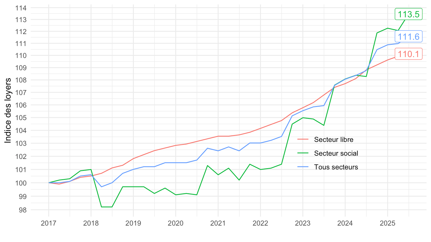
INDICES_LOYERS |>
  filter(REF_AREA == "PR",
         NATURE == "INDICE") |>
  quarter_to_date() |>
  ggplot() + ylab("Indice des loyers") + xlab("") + theme_minimal() +
  geom_line(aes(x = date, y = OBS_VALUE, color = Secteurs_loyers)) +

  scale_x_date(breaks = seq(1920, 2100, 5) |> paste0("-01-01") |> as.Date(),
               labels = date_format("%Y")) +
  theme(legend.position = c(0.75, 0.3),
        legend.title = element_blank()) +
  scale_y_log10(breaks = seq(0, 400, 10),
                     labels = dollar_format(accuracy = 1, prefix = ""))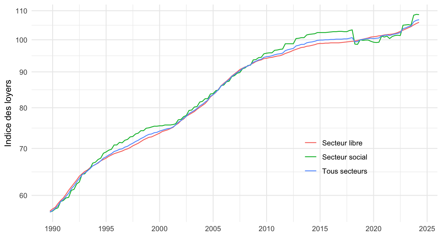
INDICES_LOYERS |>
  filter(REF_AREA == "FR-D976",
         NATURE == "INDICE") |>
  quarter_to_date() |>
  ggplot() + ylab("Indice des loyers") + xlab("") + theme_minimal() +
  geom_line(aes(x = date, y = OBS_VALUE, color = Secteurs_loyers)) +

  scale_x_date(breaks = seq(1920, 2100, 1) |> paste0("-01-01") |> as.Date(),
               labels = date_format("%Y")) +
  theme(legend.position = c(0.75, 0.3),
        legend.title = element_blank()) +
  scale_y_log10(breaks = seq(0, 400, 1),
                     labels = dollar_format(accuracy = 1, prefix = ""))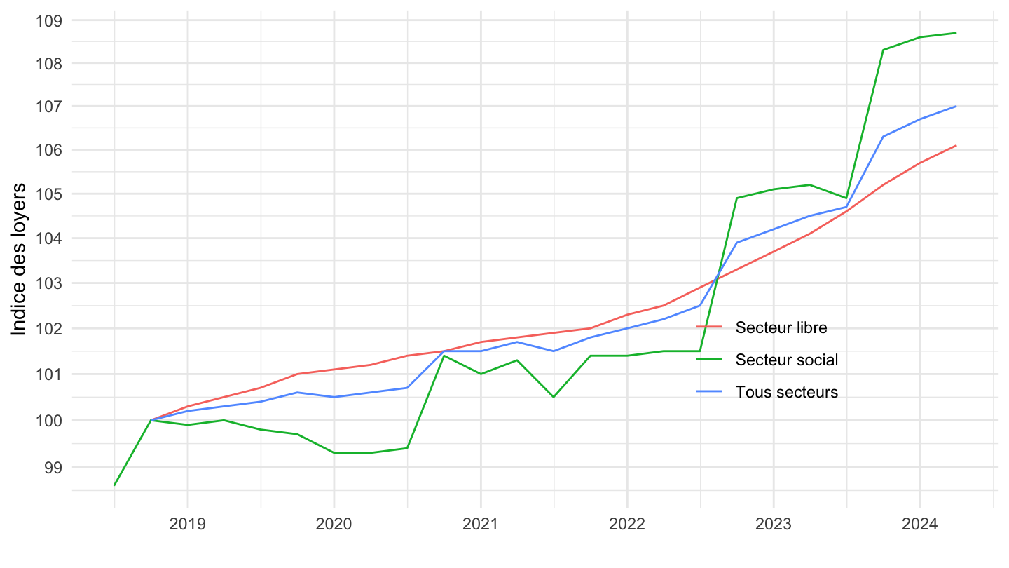
Indices des loyers d’habitation (ILH). html
Enquête Loyers et charges. html
Questionnaire de l’enquête. pdf
Qualité de l’enquête relative à l’exercice 2018. pdf
Les données sont calculées à partir des résultats de l’enquête Loyers et charges et de celle sur les loyers auprès des bailleurs sociaux (ELBS). Le champ recouvre l’ensemble des résidences principales, louées vides, dont l’usage principal est l’habitation. L’indice est calculé selon la formule de Laspeyres appliquée à des loyers au mètre carré. On mesure une évolution à qualité constante, en rapportant les loyers du parc observés au trimestre T aux loyers du parc observés au trimestre T-1. Ces indices sont ensuite chaînés, du 1er mois d’un trimestre au 1er mois du trimestre précédent.
Ces données diffèrent de l’indice de référence des loyers (IRL), qui constitue la référence pour la révision des loyers en cours de bail dans le parc locatif privé, car l’évolution des loyers présentée ici est celle effectivement constatée. Si la variation réelle des loyers est corrélée à l’évolution de l’IRL, les deux indices ne sont cependant pas identiques.
| source | dataset | Title | Updated |
|---|---|---|---|
| source | dataset | Title | Updated |
|---|---|---|---|
| source | dataset | Title | Updated |
|---|---|---|---|
| source | dataset | Title | Updated |
|---|---|---|---|