| date | Nobs |
|---|---|
| 2026-05-01 | 86 |
Consumer Price Index
Data - BIS
Info
Last
iso3c, iso2c, Reference area
Code
CPI %>%
  arrange(iso3c, date) %>%
  group_by(iso3c, iso2c, `Reference area`) %>%
  summarise(Nobs = n(),
            start = first(date),
            end = last(date)) %>%
  arrange(-Nobs) %>%
  mutate(Flag = gsub(" ", "-", str_to_lower(`Reference area`)),
         Flag = paste0('<img src="../../icon/flag/vsmall/', Flag, '.png" alt="Flag">')) %>%
  select(Flag, everything()) %>%
  {if (is_html_output()) datatable(., filter = 'top', rownames = F, escape = F) else .}
FREQ, Frequency
Code
CPI %>%
  group_by(FREQ, Frequency) %>%
  summarise(Nobs = n()) %>%
  arrange(-Nobs) %>%
{if (is_html_output()) print_table(.) else .}| FREQ | Frequency | Nobs |
|---|---|---|
| M | Monthly | 95265 |
| A | Annual | 9523 |
UNIT_MEASURE, Unit of measure
Code
CPI %>%
  group_by(UNIT_MEASURE, `Unit of measure`) %>%
  summarise(Nobs = n()) %>%
  arrange(-Nobs) %>%
{if (is_html_output()) print_table(.) else .}| UNIT_MEASURE | Unit of measure | Nobs |
|---|---|---|
| 628 | Index, 2010 = 100 | 52812 |
| 771 | Year-on-year changes, in per cent | 51976 |
Year-on-year changes
Table - How much data on Inflation ?
Code
CPI %>%
  filter(UNIT_MEASURE == 771,
         FREQ == "A") %>%
  group_by(iso3c, iso2c, `Reference area`) %>%
  summarise(Nobs = n(),
            start = first(date),
            end = last(date)) %>%
  arrange(-Nobs) %>%
  mutate(Flag = gsub(" ", "-", str_to_lower(`Reference area`)),
         Flag = paste0('<img src="../../icon/flag/vsmall/', Flag, '.png" alt="Flag">')) %>%
  select(Flag, everything()) %>%
  {if (is_html_output()) datatable(., filter = 'top', rownames = F, escape = F) else .}
United Kingdom
Code
CPI %>%
  filter(iso3c %in% c("GBR"),
         UNIT_MEASURE == 771,
         FREQ == "A") %>%
  ggplot(.) + geom_line() + theme_minimal() +
  aes(x = date, y = value/100) + xlab("") + ylab("Inflation") +
  scale_x_date(breaks = seq(1600, 2100, 50) %>% paste0("-01-01") %>% as.Date,
               labels = date_format("%Y")) +
  scale_y_continuous(breaks = 0.01*seq(-100, 200, 5),
                     labels = percent_format(a = 1)) +
  geom_hline(yintercept = 0, linetype = "dashed", color = "grey")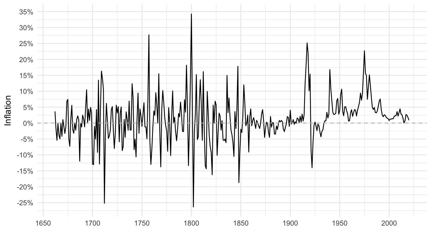
United Kingdom (1952-)
Code
CPI %>%
  filter(iso3c %in% c("GBR"),
         date >= as.Date("1952-01-01"),
         UNIT_MEASURE == 771,
         FREQ == "A") %>%
  ggplot(.) + geom_line() + theme_minimal() +
  aes(x = date, y = value/100) + xlab("") + ylab("Inflation") +
  scale_x_date(breaks = seq(1900, 2100, 5) %>% paste0("-01-01") %>% as.Date,
               labels = date_format("%Y")) +
  scale_y_continuous(breaks = 0.01*seq(-10, 200, 2),
                     labels = percent_format(a = 1)) +
  geom_hline(yintercept = 0, linetype = "dashed", color = "grey")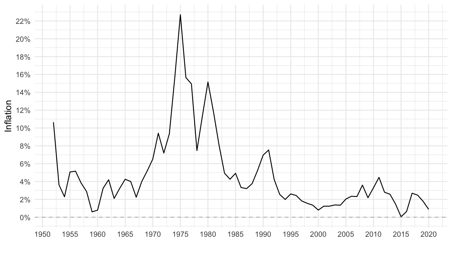
United States
Code
CPI %>%
  filter(iso3c %in% c("USA"),
         UNIT_MEASURE == 771,
         FREQ == "A") %>%
  ggplot(.) + geom_line() + theme_minimal() +
  aes(x = date, y = value/100) + xlab("") + ylab("Inflation") +
  scale_x_date(breaks = seq(1900, 2100, 10) %>% paste0("-01-01") %>% as.Date,
               labels = date_format("%Y")) +
  scale_y_continuous(breaks = 0.01*seq(-10, 200, 2),
                     labels = percent_format(a = 1)) +
  geom_hline(yintercept = 0, linetype = "dashed", color = "grey")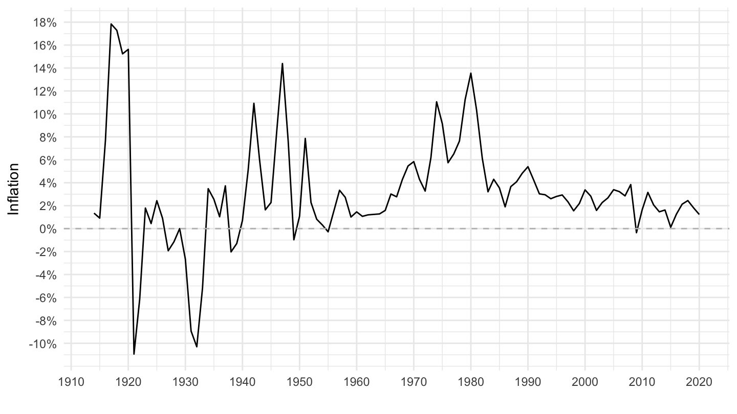
United States (1952-)
Code
CPI %>%
  filter(iso3c %in% c("USA"),
         date >= as.Date("1952-01-01"),
         UNIT_MEASURE == 771,
         FREQ == "A") %>%
  ggplot(.) + geom_line() + theme_minimal() +
  aes(x = date, y = value/100) + xlab("") + ylab("Inflation") +
  scale_x_date(breaks = seq(1900, 2100, 5) %>% paste0("-01-01") %>% as.Date,
               labels = date_format("%Y")) +
  scale_y_continuous(breaks = 0.01*seq(-10, 200, 2),
                     labels = percent_format(a = 1)) +
  geom_hline(yintercept = 0, linetype = "dashed", color = "grey")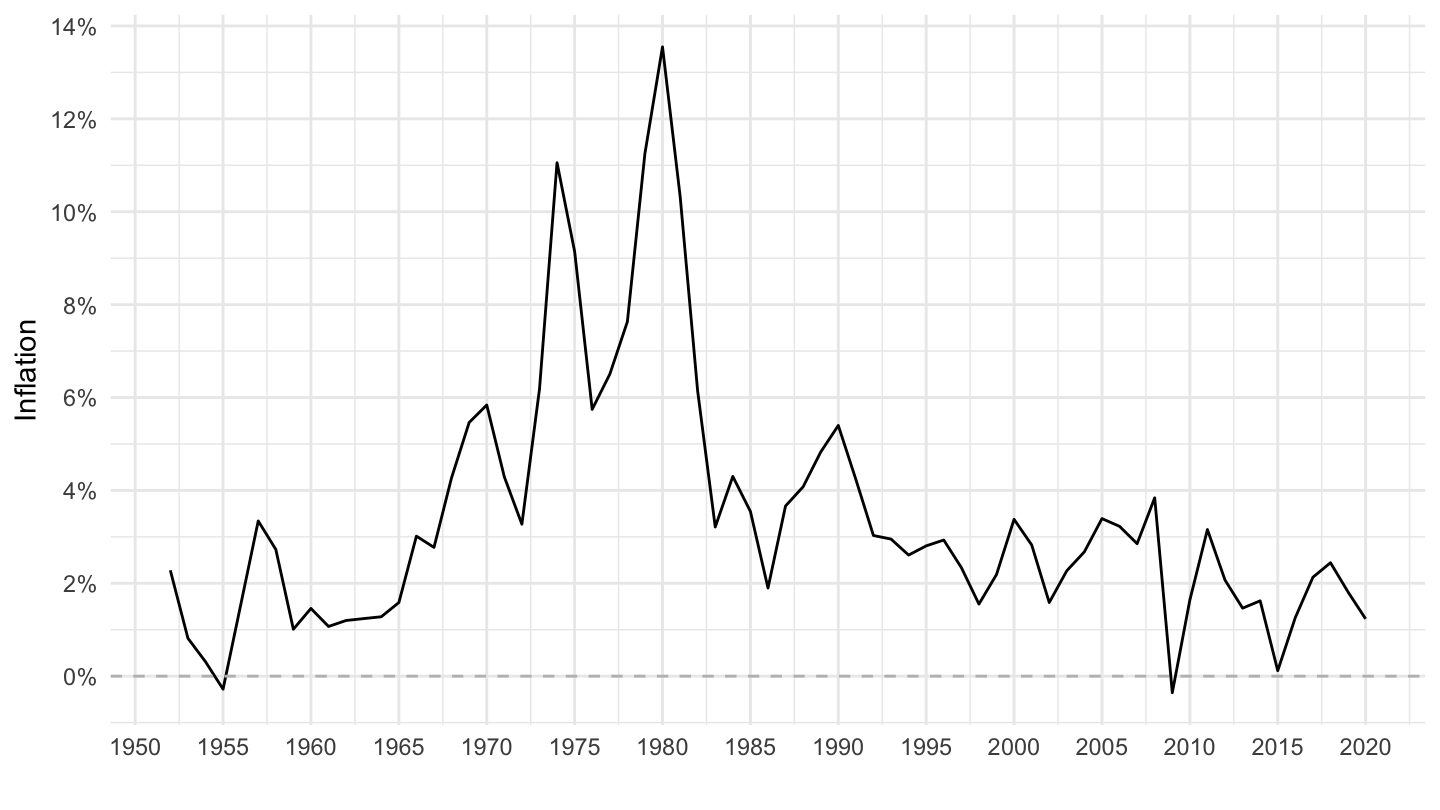
Canada
Code
CPI %>%
  filter(iso3c %in% c("CAN"),
         UNIT_MEASURE == 771,
         FREQ == "A") %>%
  ggplot(.) + geom_line() + theme_minimal() +
  aes(x = date, y = value/100) + xlab("") + ylab("Inflation") +
  scale_x_date(breaks = seq(1900, 2100, 10) %>% paste0("-01-01") %>% as.Date,
               labels = date_format("%Y")) +
  scale_y_continuous(breaks = 0.01*seq(-10, 200, 2),
                     labels = percent_format(a = 1)) +
  geom_hline(yintercept = 0, linetype = "dashed", color = "grey")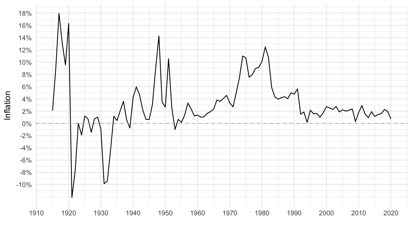
Canada (1952-)
Code
CPI %>%
  filter(iso3c %in% c("CAN"),
         date >= as.Date("1952-01-01"),
         UNIT_MEASURE == 771,
         FREQ == "A") %>%
  ggplot(.) + geom_line() + theme_minimal() +
  aes(x = date, y = value/100) + xlab("") + ylab("Inflation") +
  scale_x_date(breaks = seq(1900, 2100, 5) %>% paste0("-01-01") %>% as.Date,
               labels = date_format("%Y")) +
  scale_y_continuous(breaks = 0.01*seq(-10, 200, 2),
                     labels = percent_format(a = 1)) +
  geom_hline(yintercept = 0, linetype = "dashed", color = "grey")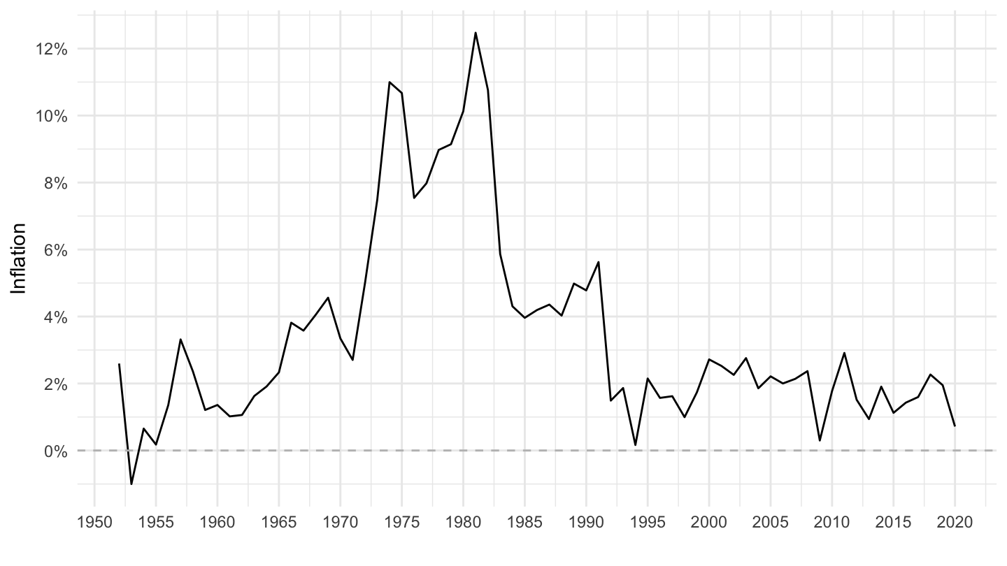
Norway
Code
CPI %>%
  filter(iso3c %in% c("NOR"),
         UNIT_MEASURE == 771,
         FREQ == "A") %>%
  ggplot(.) + geom_line() + theme_minimal() +
  aes(x = date, y = value/100) + xlab("") + ylab("Inflation") +
  scale_x_date(breaks = seq(1800, 2100, 20) %>% paste0("-01-01") %>% as.Date,
               labels = date_format("%Y")) +
  scale_y_continuous(breaks = 0.01*seq(-100, 200, 5),
                     labels = percent_format(a = 1)) +
  geom_hline(yintercept = 0, linetype = "dashed", color = "grey")
Norway (1952-)
Code
CPI %>%
  filter(iso3c %in% c("NOR"),
         date >= as.Date("1952-01-01"),
         UNIT_MEASURE == 771,
         FREQ == "A") %>%
  ggplot(.) + geom_line() + theme_minimal() +
  aes(x = date, y = value/100) + xlab("") + ylab("Inflation") +
  scale_x_date(breaks = seq(1900, 2100, 5) %>% paste0("-01-01") %>% as.Date,
               labels = date_format("%Y")) +
  scale_y_continuous(breaks = 0.01*seq(-10, 200, 2),
                     labels = percent_format(a = 1)) +
  geom_hline(yintercept = 0, linetype = "dashed", color = "grey")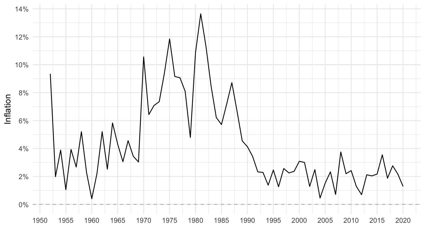
Switzerland
Code
CPI %>%
  filter(iso3c %in% c("CHE"),
         UNIT_MEASURE == 771,
         FREQ == "A") %>%
  ggplot(.) + geom_line() + theme_minimal() +
  aes(x = date, y = value/100) + xlab("") + ylab("Inflation") +
  scale_x_date(breaks = seq(1800, 2100, 20) %>% paste0("-01-01") %>% as.Date,
               labels = date_format("%Y")) +
  scale_y_continuous(breaks = 0.01*seq(-100, 200, 5),
                     labels = percent_format(a = 1)) +
  geom_hline(yintercept = 0, linetype = "dashed", color = "grey")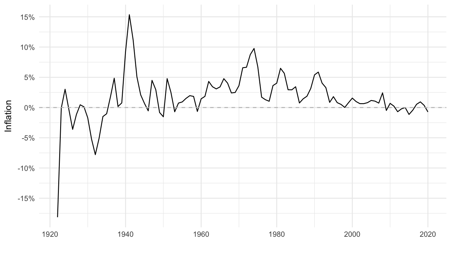
Switzerland (1952-)
Code
CPI %>%
  filter(iso3c %in% c("CHE"),
         date >= as.Date("1952-01-01"),
         UNIT_MEASURE == 771,
         FREQ == "A") %>%
  ggplot(.) + geom_line() + theme_minimal() +
  aes(x = date, y = value/100) + xlab("") + ylab("Inflation") +
  scale_x_date(breaks = seq(1900, 2100, 5) %>% paste0("-01-01") %>% as.Date,
               labels = date_format("%Y")) +
  scale_y_continuous(breaks = 0.01*seq(-10, 200, 2),
                     labels = percent_format(a = 1)) +
  geom_hline(yintercept = 0, linetype = "dashed", color = "grey")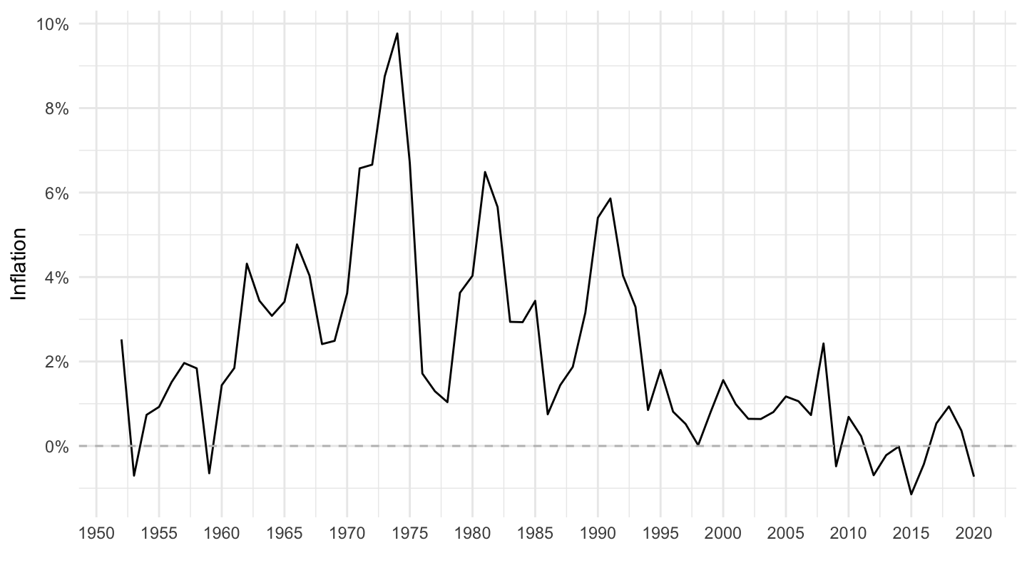
Switzerland (2010-)
Code
CPI %>%
  filter(iso3c %in% c("CHE"),
         date >= as.Date("2010-01-01"),
         UNIT_MEASURE == 771,
         FREQ == "A") %>%
  ggplot(.) + geom_line() + theme_minimal() +
  aes(x = date, y = value/100) + xlab("") + ylab("Inflation") +
  scale_x_date(breaks = seq(1900, 2100, 1) %>% paste0("-01-01") %>% as.Date,
               labels = date_format("%Y")) +
  scale_y_continuous(breaks = 0.01*seq(-10, 200, 0.2),
                     labels = percent_format(a = .2)) +
  geom_hline(yintercept = 0, linetype = "dashed", color = "grey")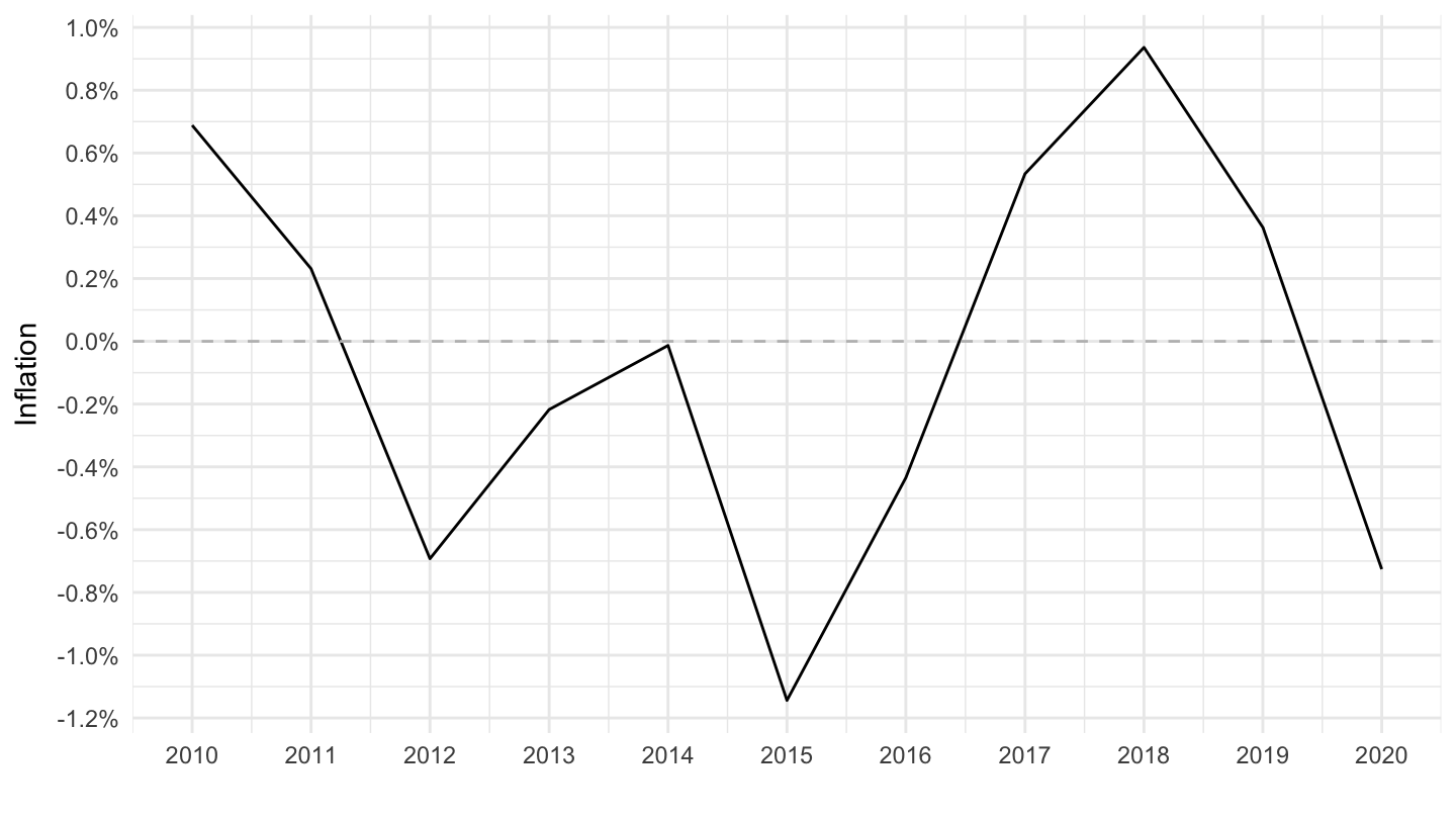
Denmark
Code
CPI %>%
  filter(iso3c %in% c("DNK"),
         UNIT_MEASURE == 771,
         FREQ == "A") %>%
  ggplot(.) + geom_line() + theme_minimal() +
  aes(x = date, y = value/100) + xlab("") + ylab("Inflation") +
  scale_x_date(breaks = seq(1800, 2100, 20) %>% paste0("-01-01") %>% as.Date,
               labels = date_format("%Y")) +
  scale_y_continuous(breaks = 0.01*seq(-100, 200, 5),
                     labels = percent_format(a = 1)) +
  geom_hline(yintercept = 0, linetype = "dashed", color = "grey")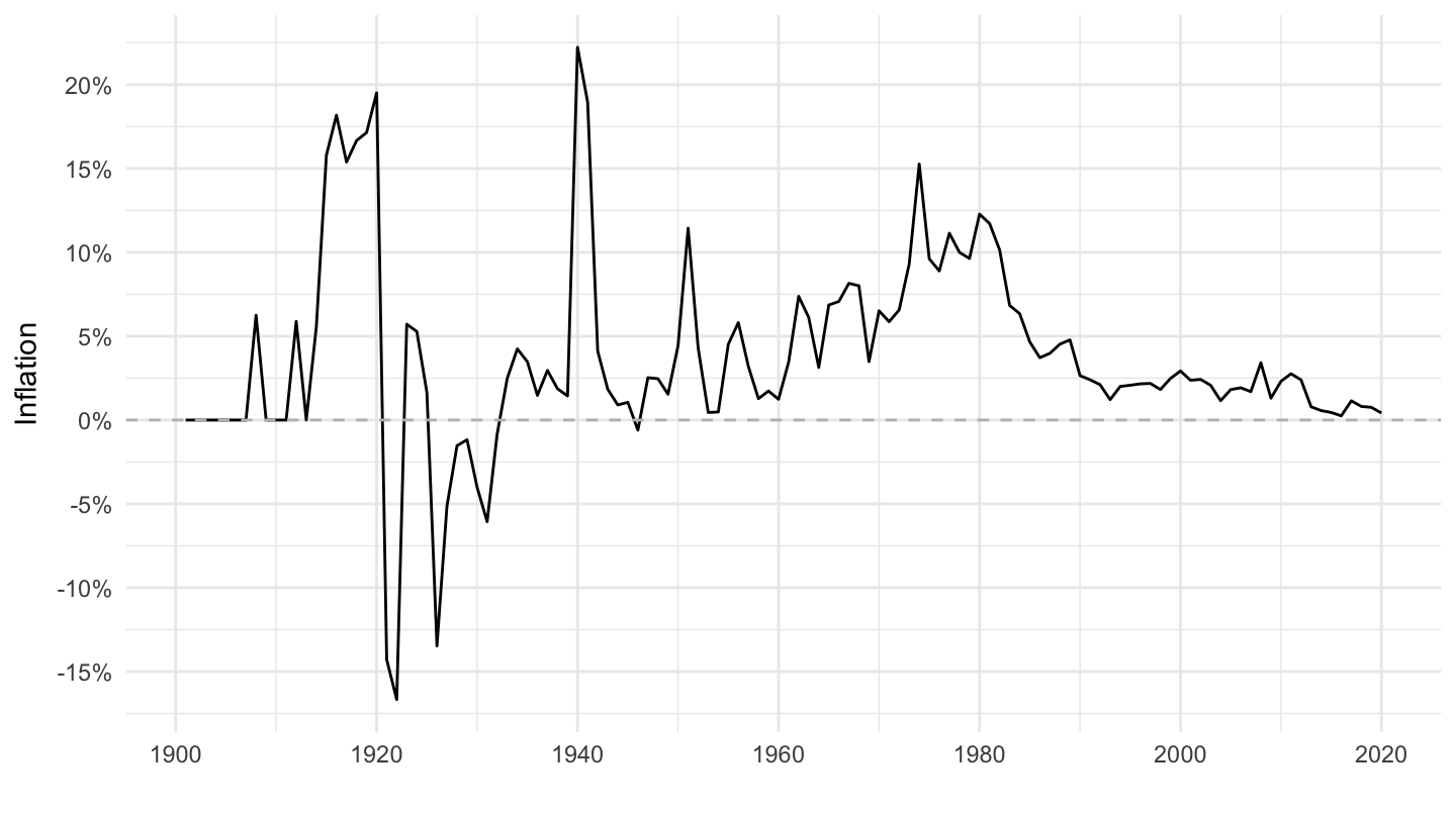
Denmark (1952-)
Code
CPI %>%
  filter(iso3c %in% c("DNK"),
         date >= as.Date("1952-01-01"),
         UNIT_MEASURE == 771,
         FREQ == "A") %>%
  ggplot(.) + geom_line() + theme_minimal() +
  aes(x = date, y = value/100) + xlab("") + ylab("Inflation") +
  scale_x_date(breaks = seq(1900, 2100, 5) %>% paste0("-01-01") %>% as.Date,
               labels = date_format("%Y")) +
  scale_y_continuous(breaks = 0.01*seq(-10, 200, 2),
                     labels = percent_format(a = 1)) +
  geom_hline(yintercept = 0, linetype = "dashed", color = "grey")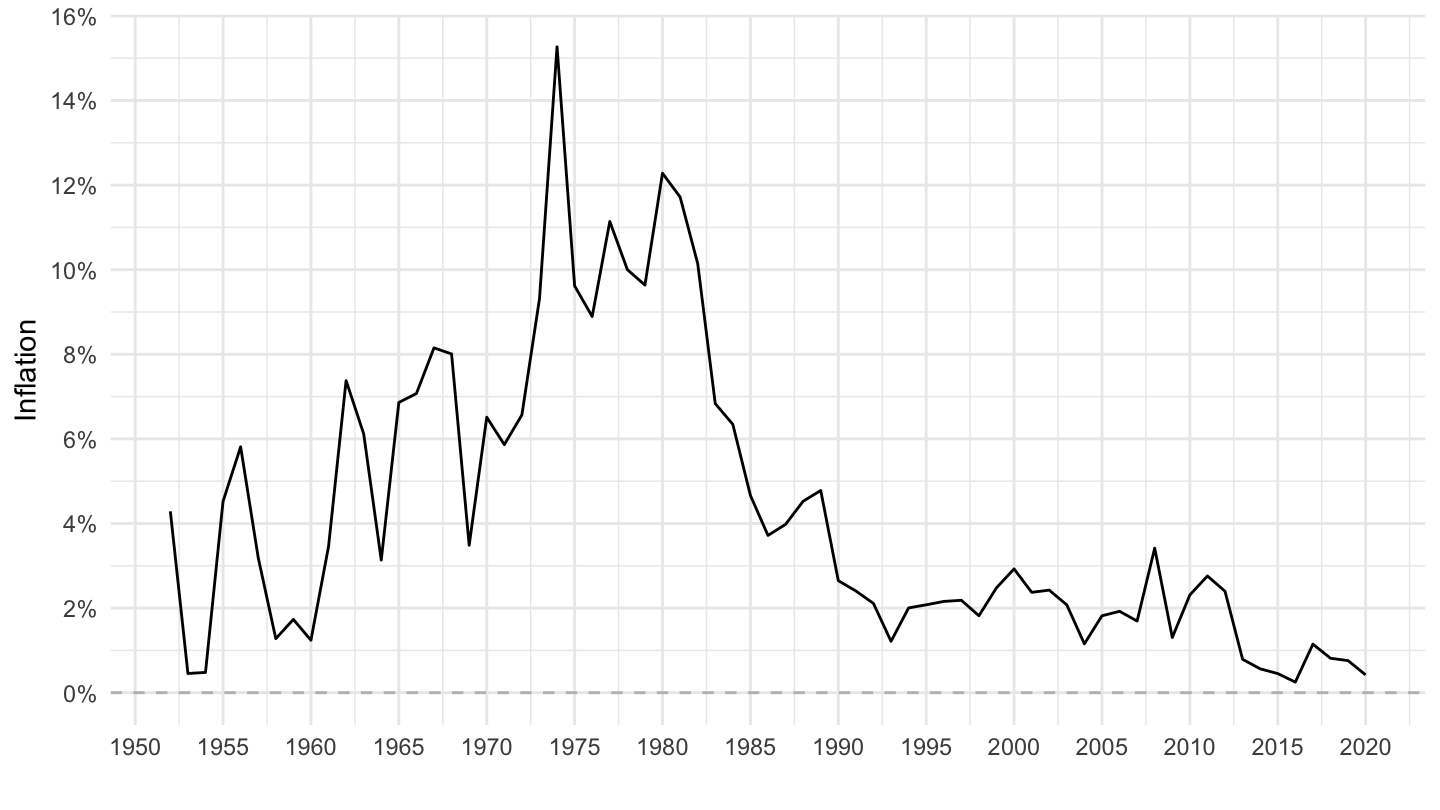
South Africa
Code
CPI %>%
  filter(iso3c %in% c("ZAF"),
         UNIT_MEASURE == 771,
         FREQ == "A") %>%
  ggplot(.) + geom_line() + theme_minimal() +
  aes(x = date, y = value/100) + xlab("") + ylab("Inflation") +
  scale_x_date(breaks = seq(1800, 2100, 20) %>% paste0("-01-01") %>% as.Date,
               labels = date_format("%Y")) +
  scale_y_continuous(breaks = 0.01*seq(-100, 200, 5),
                     labels = percent_format(a = 1)) +
  geom_hline(yintercept = 0, linetype = "dashed", color = "grey")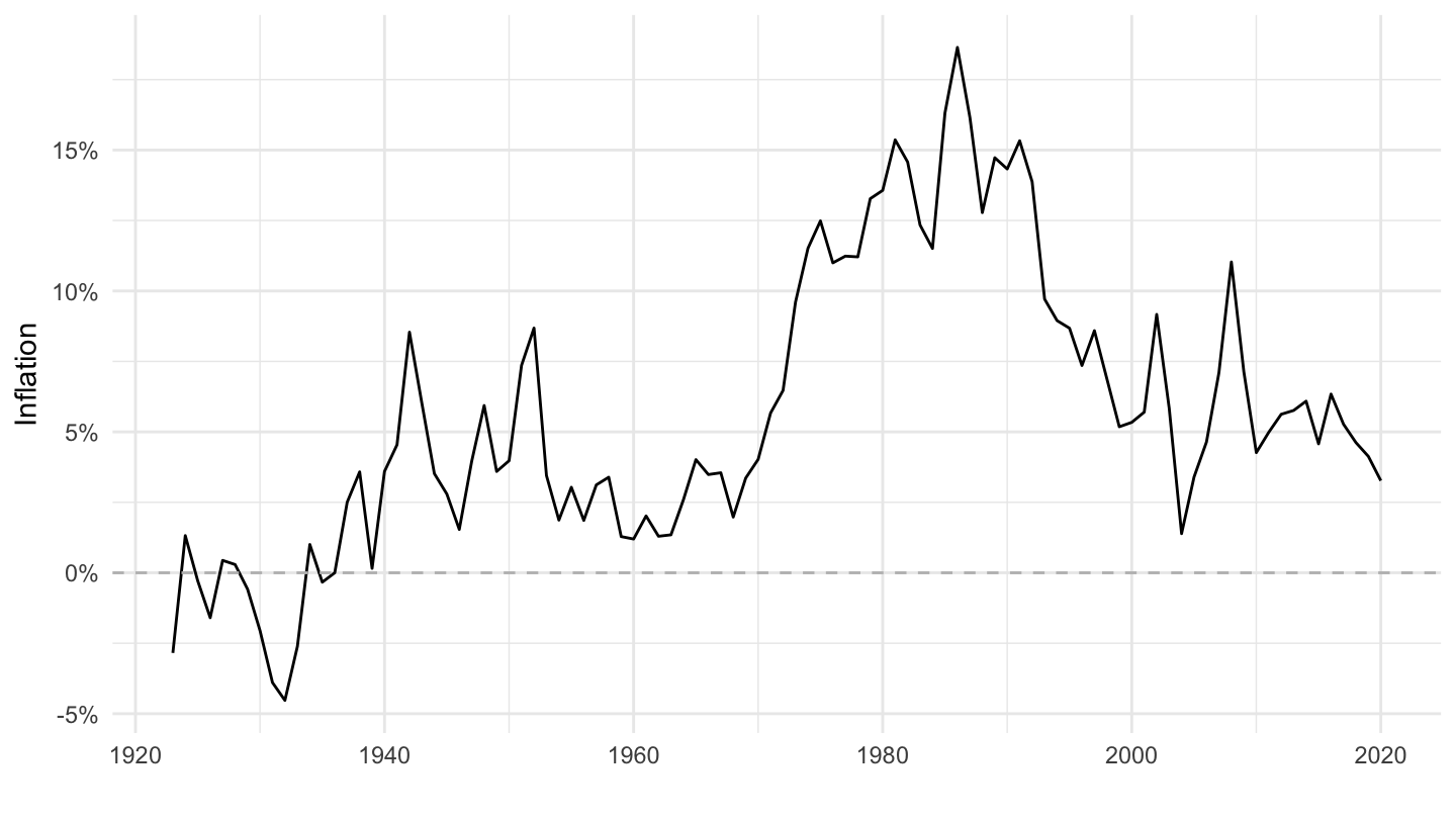
South Africa (1952-)
Code
CPI %>%
  filter(iso3c %in% c("ZAF"),
         date >= as.Date("1952-01-01"),
         UNIT_MEASURE == 771,
         FREQ == "A") %>%
  ggplot(.) + geom_line() + theme_minimal() +
  aes(x = date, y = value/100) + xlab("") + ylab("Inflation") +
  scale_x_date(breaks = seq(1900, 2100, 5) %>% paste0("-01-01") %>% as.Date,
               labels = date_format("%Y")) +
  scale_y_continuous(breaks = 0.01*seq(-10, 200, 2),
                     labels = percent_format(a = 1)) +
  geom_hline(yintercept = 0, linetype = "dashed", color = "grey")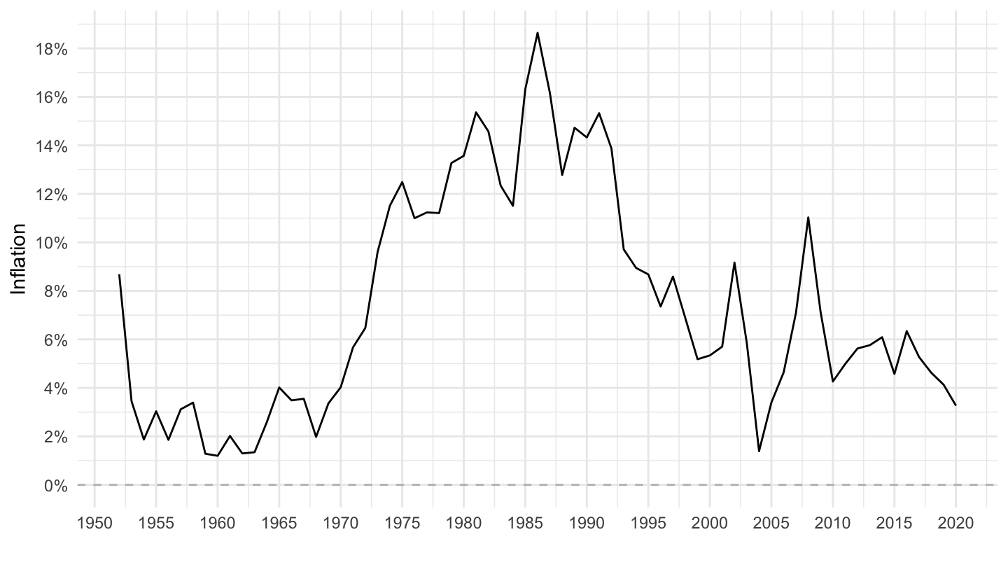
Belgium
Code
CPI %>%
  filter(iso3c %in% c("BEL"),
         UNIT_MEASURE == 771,
         FREQ == "A") %>%
  ggplot(.) + geom_line() + theme_minimal() +
  aes(x = date, y = value/100) + xlab("") + ylab("Inflation") +
  scale_x_date(breaks = seq(1800, 2100, 20) %>% paste0("-01-01") %>% as.Date,
               labels = date_format("%Y")) +
  scale_y_continuous(breaks = 0.01*seq(-100, 200, 5),
                     labels = percent_format(a = 1)) +
  geom_hline(yintercept = 0, linetype = "dashed", color = "grey")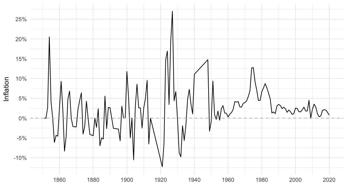
Belgium (1952-)
Code
CPI %>%
  filter(iso3c %in% c("BEL"),
         date >= as.Date("1952-01-01"),
         UNIT_MEASURE == 771,
         FREQ == "A") %>%
  ggplot(.) + geom_line() + theme_minimal() +
  aes(x = date, y = value/100) + xlab("") + ylab("Inflation") +
  scale_x_date(breaks = seq(1900, 2100, 5) %>% paste0("-01-01") %>% as.Date,
               labels = date_format("%Y")) +
  scale_y_continuous(breaks = 0.01*seq(-10, 200, 2),
                     labels = percent_format(a = 1)) +
  geom_hline(yintercept = 0, linetype = "dashed", color = "grey")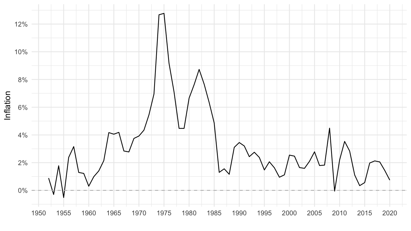
Australia
Code
CPI %>%
  filter(iso3c %in% c("AUS"),
         UNIT_MEASURE == 771,
         FREQ == "A") %>%
  ggplot(.) + geom_line() + theme_minimal() +
  aes(x = date, y = value/100) + xlab("") + ylab("Inflation") +
  scale_x_date(breaks = seq(1800, 2100, 20) %>% paste0("-01-01") %>% as.Date,
               labels = date_format("%Y")) +
  scale_y_continuous(breaks = 0.01*seq(-100, 200, 5),
                     labels = percent_format(a = 1)) +
  geom_hline(yintercept = 0, linetype = "dashed", color = "grey")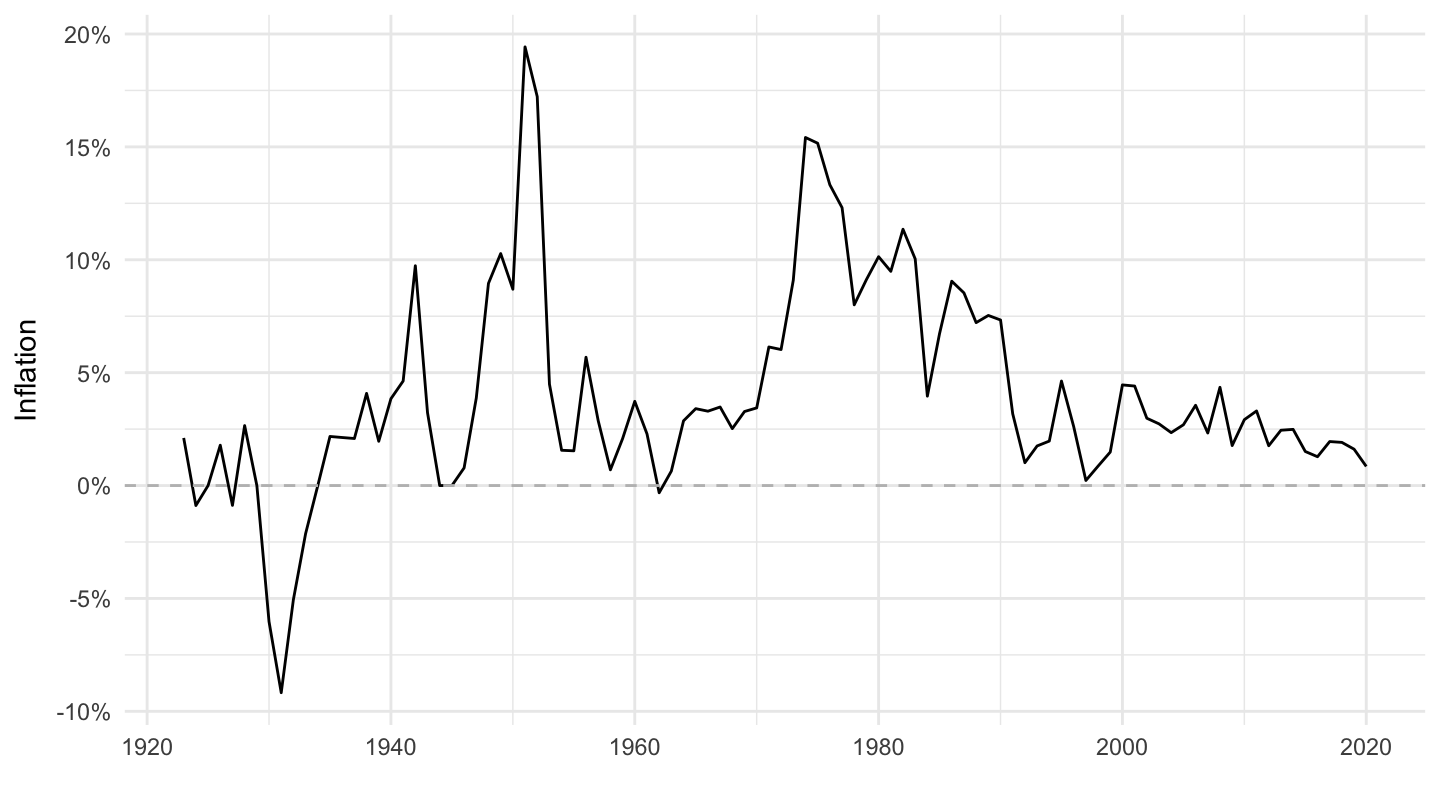
Australia (1952-)
Code
CPI %>%
  filter(iso3c %in% c("AUS"),
         date >= as.Date("1952-01-01"),
         UNIT_MEASURE == 771,
         FREQ == "A") %>%
  ggplot(.) + geom_line() + theme_minimal() +
  aes(x = date, y = value/100) + xlab("") + ylab("Inflation") +
  scale_x_date(breaks = seq(1900, 2100, 5) %>% paste0("-01-01") %>% as.Date,
               labels = date_format("%Y")) +
  scale_y_continuous(breaks = 0.01*seq(-10, 200, 2),
                     labels = percent_format(a = 1)) +
  geom_hline(yintercept = 0, linetype = "dashed", color = "grey")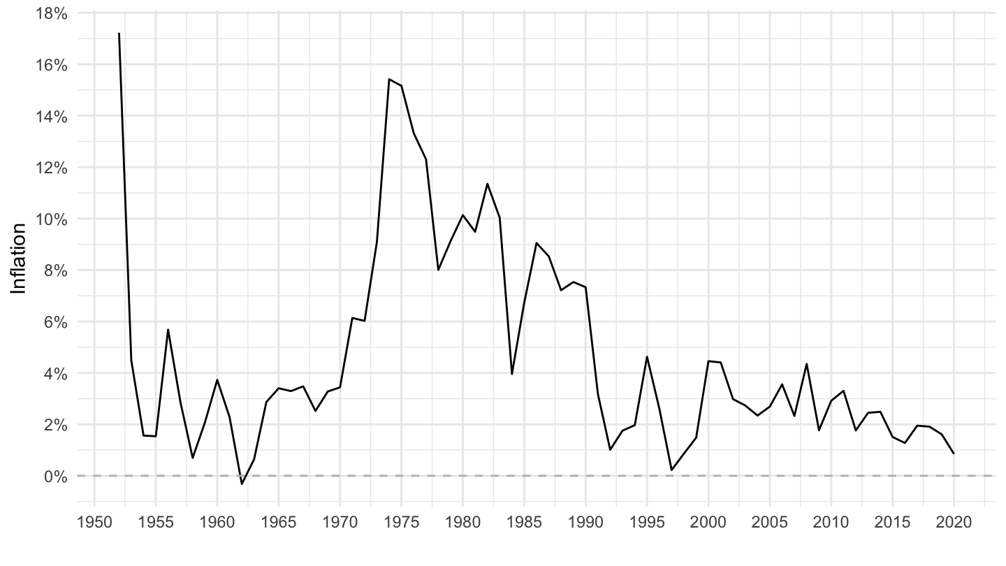
New Zealand
Code
CPI %>%
  filter(iso3c %in% c("NZL"),
         UNIT_MEASURE == 771,
         FREQ == "A") %>%
  ggplot(.) + geom_line() + theme_minimal() +
  aes(x = date, y = value/100) + xlab("") + ylab("Inflation") +
  scale_x_date(breaks = seq(1800, 2100, 20) %>% paste0("-01-01") %>% as.Date,
               labels = date_format("%Y")) +
  scale_y_continuous(breaks = 0.01*seq(-100, 200, 5),
                     labels = percent_format(a = 1)) +
  geom_hline(yintercept = 0, linetype = "dashed", color = "grey")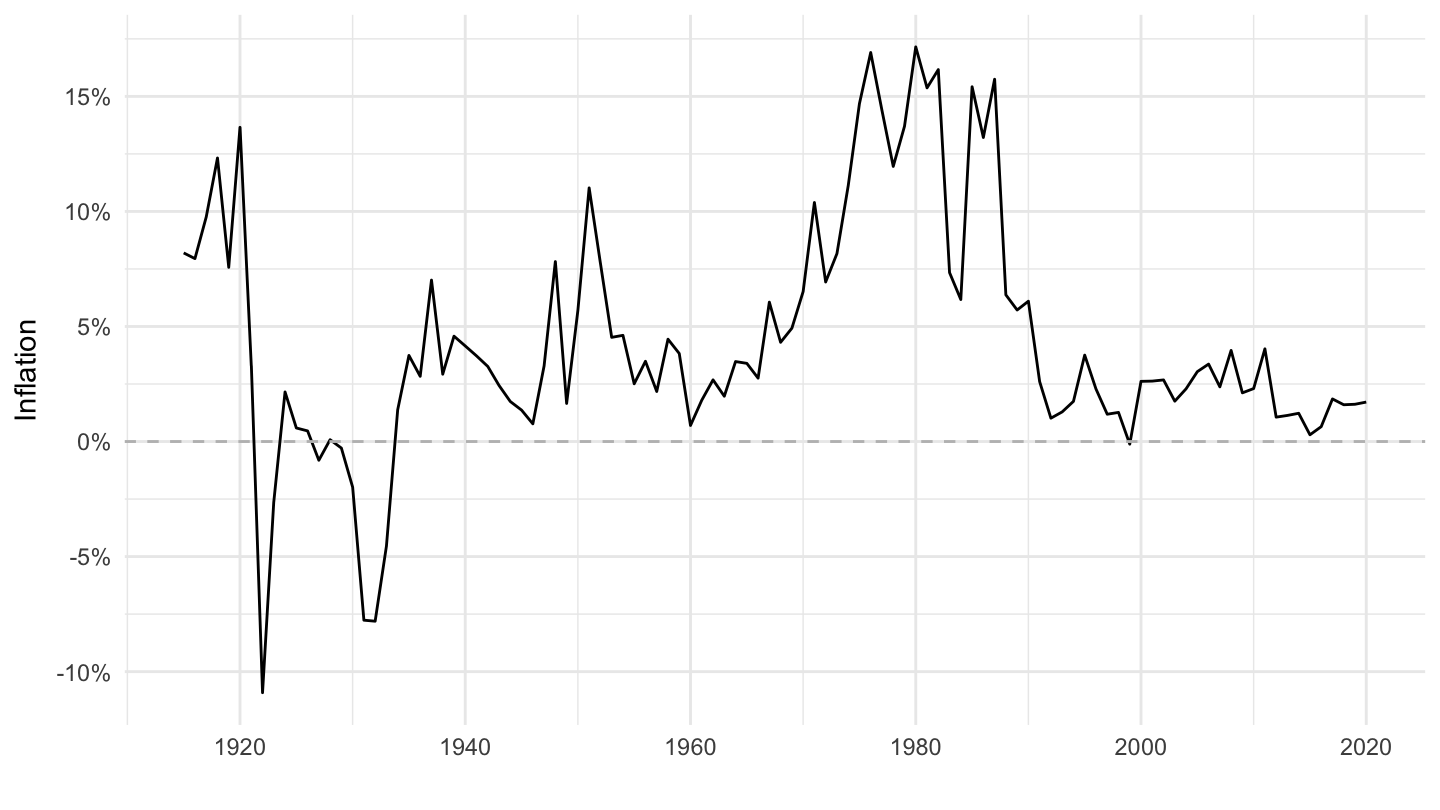
New Zealand (1952-)
Code
CPI %>%
  filter(iso3c %in% c("NZL"),
         date >= as.Date("1952-01-01"),
         UNIT_MEASURE == 771,
         FREQ == "A") %>%
  ggplot(.) + geom_line() + theme_minimal() +
  aes(x = date, y = value/100) + xlab("") + ylab("Inflation") +
  scale_x_date(breaks = seq(1900, 2100, 5) %>% paste0("-01-01") %>% as.Date,
               labels = date_format("%Y")) +
  scale_y_continuous(breaks = 0.01*seq(-10, 200, 2),
                     labels = percent_format(a = 1)) +
  geom_hline(yintercept = 0, linetype = "dashed", color = "grey")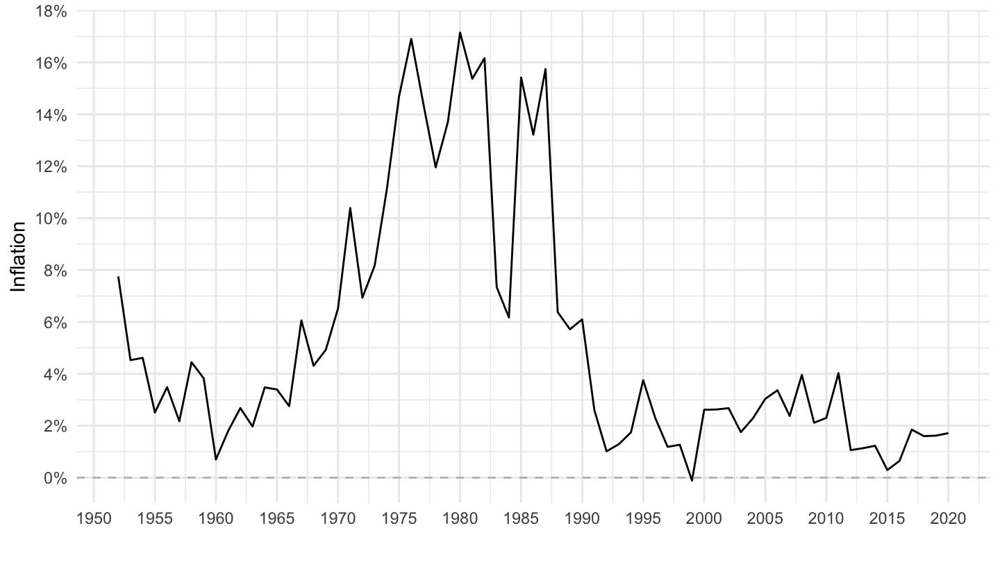
Ireland
Code
CPI %>%
  filter(iso3c %in% c("IRL"),
         UNIT_MEASURE == 771,
         FREQ == "A") %>%
  ggplot(.) + geom_line() + theme_minimal() +
  aes(x = date, y = value/100) + xlab("") + ylab("Inflation") +
  scale_x_date(breaks = seq(1800, 2100, 20) %>% paste0("-01-01") %>% as.Date,
               labels = date_format("%Y")) +
  scale_y_continuous(breaks = 0.01*seq(-100, 200, 5),
                     labels = percent_format(a = 1)) +
  geom_hline(yintercept = 0, linetype = "dashed", color = "grey")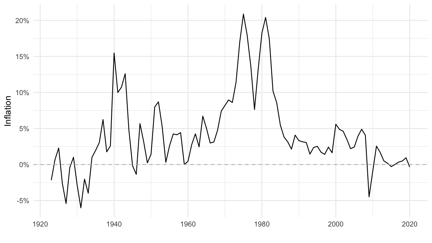
Ireland (1952-)
Code
CPI %>%
  filter(iso3c %in% c("IRL"),
         date >= as.Date("1952-01-01"),
         UNIT_MEASURE == 771,
         FREQ == "A") %>%
  ggplot(.) + geom_line() + theme_minimal() +
  aes(x = date, y = value/100) + xlab("") + ylab("Inflation") +
  scale_x_date(breaks = seq(1900, 2100, 5) %>% paste0("-01-01") %>% as.Date,
               labels = date_format("%Y")) +
  scale_y_continuous(breaks = 0.01*seq(-10, 200, 2),
                     labels = percent_format(a = 1)) +
  geom_hline(yintercept = 0, linetype = "dashed", color = "grey")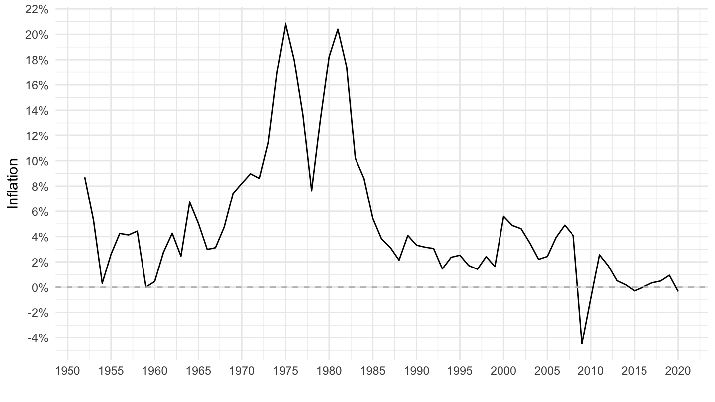
Chile
Code
CPI %>%
  filter(iso3c %in% c("ISL"),
         UNIT_MEASURE == 771,
         FREQ == "A") %>%
  ggplot(.) + geom_line() + theme_minimal() +
  aes(x = date, y = value/100) + xlab("") + ylab("Inflation") +
  scale_x_date(breaks = seq(1800, 2100, 20) %>% paste0("-01-01") %>% as.Date,
               labels = date_format("%Y")) +
  scale_y_continuous(breaks = 0.01*seq(-100, 600, 20),
                     labels = percent_format(a = 1)) +
  geom_hline(yintercept = 0, linetype = "dashed", color = "grey")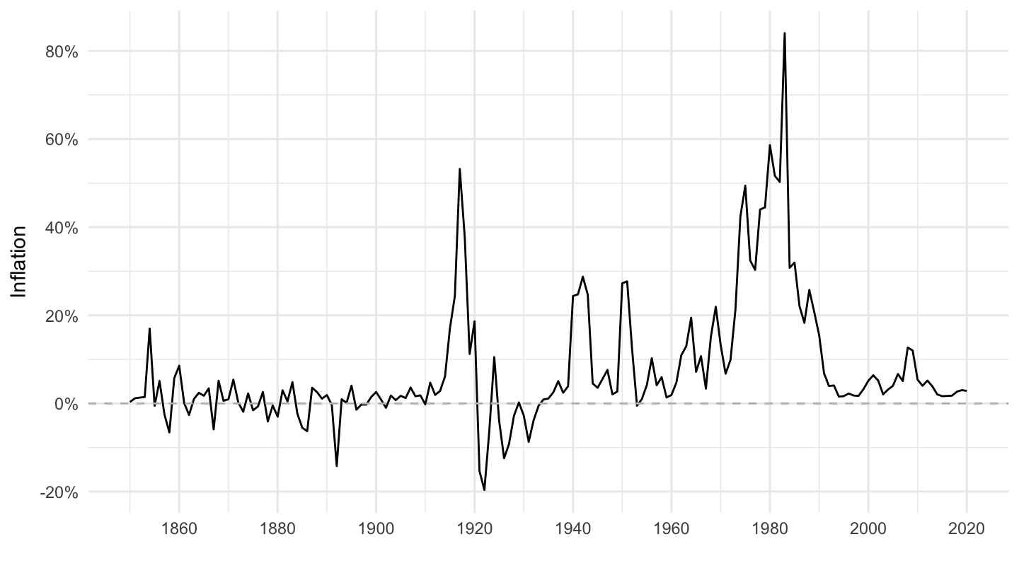
Chile (1952-)
Code
CPI %>%
  filter(iso3c %in% c("CHL"),
         date >= as.Date("1952-01-01"),
         UNIT_MEASURE == 771,
         FREQ == "A") %>%
  ggplot(.) + geom_line() + theme_minimal() +
  aes(x = date, y = value/100) + xlab("") + ylab("Inflation") +
  scale_x_date(breaks = seq(1900, 2100, 5) %>% paste0("-01-01") %>% as.Date,
               labels = date_format("%Y")) +
  scale_y_continuous(breaks = 0.01*seq(-100, 600, 20),
                     labels = percent_format(a = 1)) +
  geom_hline(yintercept = 0, linetype = "dashed", color = "grey")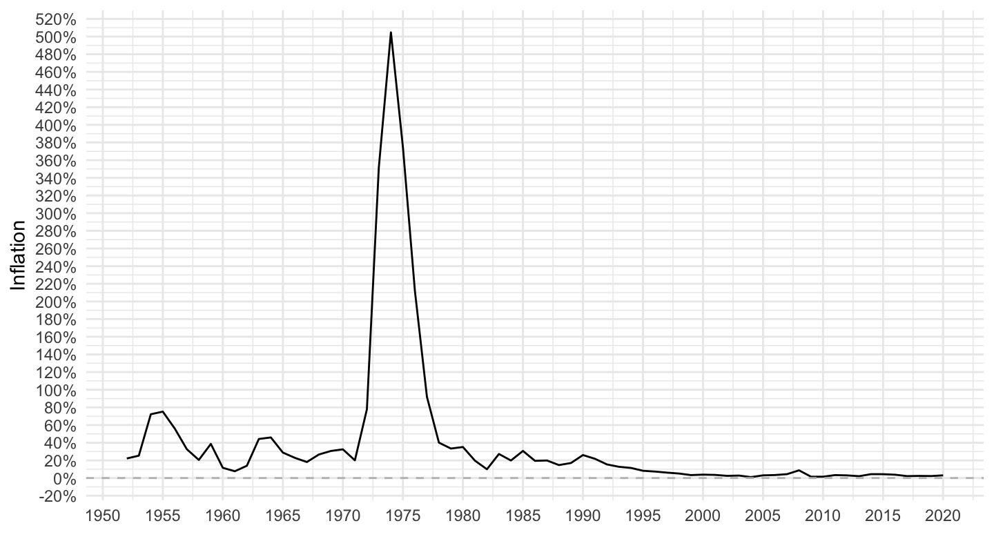
Iceland
Code
CPI %>%
  filter(iso3c %in% c("ISL"),
         UNIT_MEASURE == 771,
         FREQ == "A") %>%
  ggplot(.) + geom_line() + theme_minimal() +
  aes(x = date, y = value/100) + xlab("") + ylab("Inflation") +
  scale_x_date(breaks = seq(1800, 2100, 20) %>% paste0("-01-01") %>% as.Date,
               labels = date_format("%Y")) +
  scale_y_continuous(breaks = 0.01*seq(-100, 600, 20),
                     labels = percent_format(a = 1)) +
  geom_hline(yintercept = 0, linetype = "dashed", color = "grey")
Iceland (1952-)
Code
CPI %>%
  filter(iso3c %in% c("ISL"),
         date >= as.Date("1952-01-01"),
         UNIT_MEASURE == 771,
         FREQ == "A") %>%
  ggplot(.) + geom_line() + theme_minimal() +
  aes(x = date, y = value/100) + xlab("") + ylab("Inflation") +
  scale_x_date(breaks = seq(1900, 2100, 5) %>% paste0("-01-01") %>% as.Date,
               labels = date_format("%Y")) +
  scale_y_continuous(breaks = 0.01*seq(-100, 600, 20),
                     labels = percent_format(a = 1)) +
  geom_hline(yintercept = 0, linetype = "dashed", color = "grey")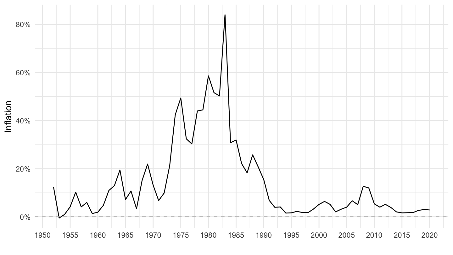
Sweden
All
Code
CPI %>%
  filter(iso3c %in% c("SWE"),
         UNIT_MEASURE == 771,
         FREQ == "A") %>%
  ggplot(.) + geom_line() + theme_minimal() +
  aes(x = date, y = value/100) + xlab("") + ylab("Inflation") +
  scale_x_date(breaks = seq(1800, 2100, 20) %>% paste0("-01-01") %>% as.Date,
               labels = date_format("%Y")) +
  scale_y_continuous(breaks = 0.01*seq(-100, 600, 10),
                     labels = percent_format(a = 1)) +
  geom_hline(yintercept = 0, linetype = "dashed", color = "grey")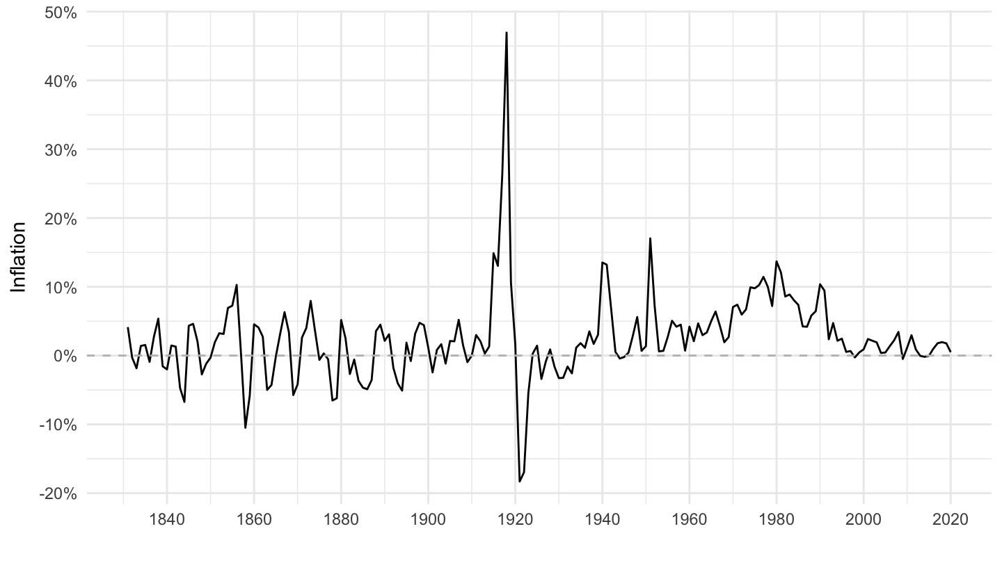
1952-
Code
CPI %>%
  filter(iso3c %in% c("SWE"),
         date >= as.Date("1952-01-01"),
         UNIT_MEASURE == 771,
         FREQ == "A") %>%
  ggplot(.) + geom_line() + theme_minimal() +
  aes(x = date, y = value/100) + xlab("") + ylab("Inflation") +
  scale_x_date(breaks = seq(1900, 2100, 5) %>% paste0("-01-01") %>% as.Date,
               labels = date_format("%Y")) +
  scale_y_continuous(breaks = 0.01*seq(-100, 600, 2),
                     labels = percent_format(a = 1)) +
  geom_hline(yintercept = 0, linetype = "dashed", color = "grey")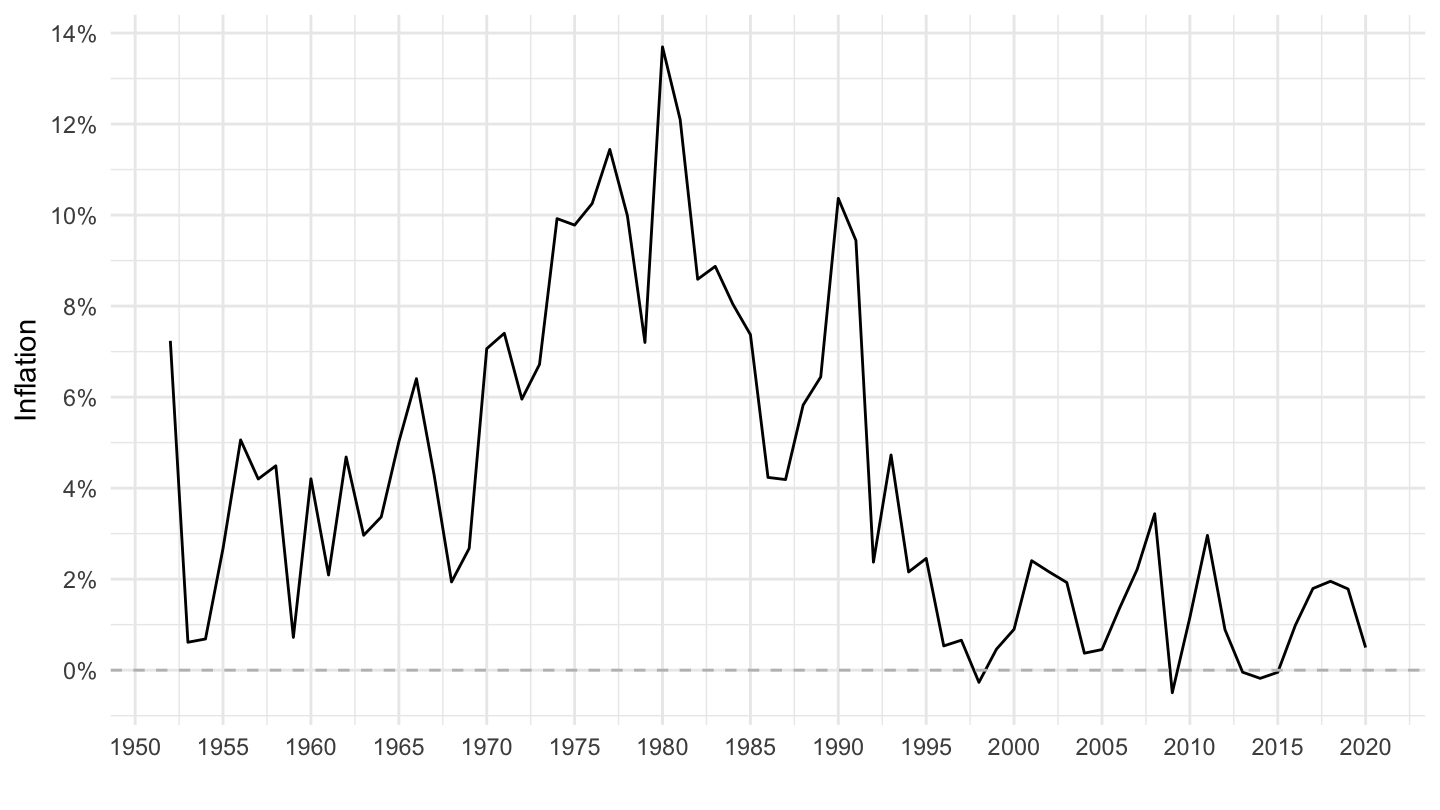
Argentina
All
Code
CPI %>%
  filter(iso3c %in% c("ARG"),
         UNIT_MEASURE == 771,
         FREQ == "A") %>%
  ggplot(.) + geom_line() + theme_minimal() +
  aes(x = date, y = value/100) + xlab("") + ylab("Inflation") +
  scale_x_date(breaks = seq(1800, 2100, 10) %>% paste0("-01-01") %>% as.Date,
               labels = date_format("%Y")) +
  scale_y_continuous(breaks = 0.01*seq(-200, 10000, 200),
                     labels = percent_format(a = 1)) +
  geom_hline(yintercept = 0, linetype = "dashed", color = "grey")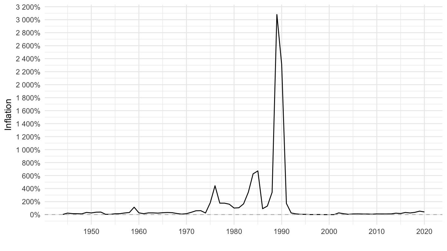
1952-
Code
CPI %>%
  filter(iso3c %in% c("ARG"),
         date >= as.Date("1952-01-01"),
         UNIT_MEASURE == 771,
         FREQ == "A") %>%
  ggplot(.) + geom_line() + theme_minimal() +
  aes(x = date, y = value/100) + xlab("") + ylab("Inflation") +
  scale_x_date(breaks = seq(1900, 2100, 5) %>% paste0("-01-01") %>% as.Date,
               labels = date_format("%Y")) +
  scale_y_continuous(breaks = 0.01*seq(-200, 10000, 200),
                     labels = percent_format(a = 1)) +
  geom_hline(yintercept = 0, linetype = "dashed", color = "grey")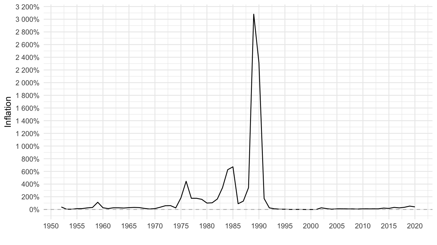
1992-
Code
CPI %>%
  filter(iso3c %in% c("ARG"),
         date >= as.Date("1992-01-01"),
         UNIT_MEASURE == 771,
         FREQ == "A") %>%
  ggplot(.) + geom_line() + theme_minimal() +
  aes(x = date, y = value/100) + xlab("") + ylab("Inflation") +
  scale_x_date(breaks = seq(1900, 2100, 2) %>% paste0("-01-01") %>% as.Date,
               labels = date_format("%Y")) +
  scale_y_continuous(breaks = 0.01*seq(-10, 80, 5),
                     labels = percent_format(a = 1)) +
  geom_hline(yintercept = 0, linetype = "dashed", color = "grey")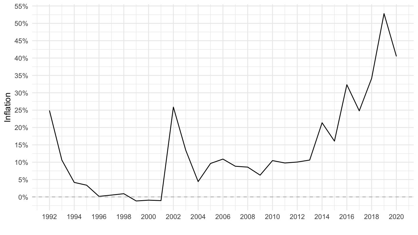
1996 - 2005
Code
CPI %>%
  filter(iso3c %in% c("ARG"),
         date >= as.Date("1996-01-01"),
         date <= as.Date("2005-01-01"),
         UNIT_MEASURE == 771,
         FREQ == "A") %>%
  ggplot(.) + geom_line() + theme_minimal() +
  aes(x = date, y = value/100) + xlab("") + ylab("Inflation") +
  scale_x_date(breaks = seq(1900, 2100, 1) %>% paste0("-01-01") %>% as.Date,
               labels = date_format("%Y")) +
  scale_y_continuous(breaks = 0.01*seq(-10, 80, 5),
                     labels = percent_format(a = 1)) +
  geom_hline(yintercept = 0, linetype = "dashed", color = "grey")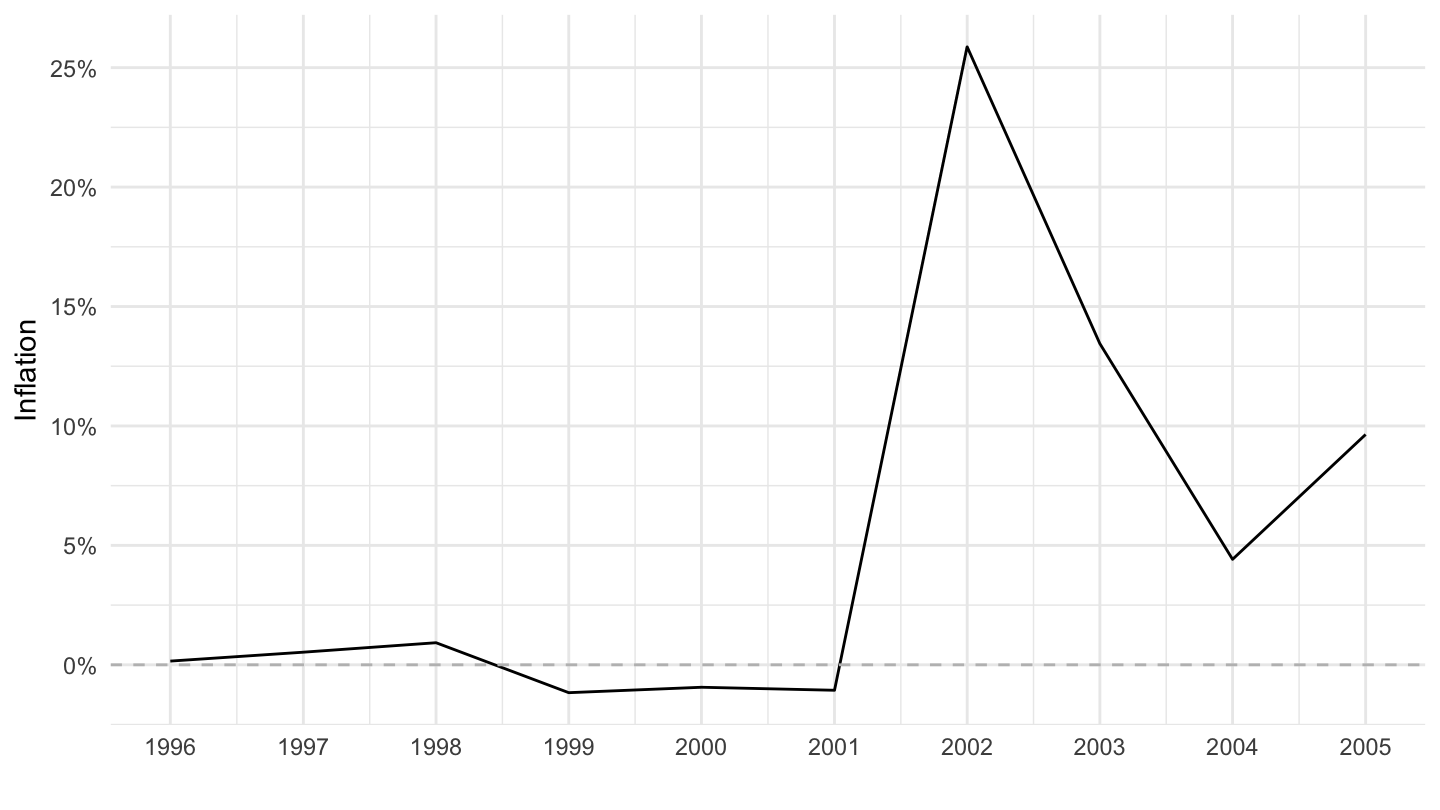
1992 - 2005
Code
CPI %>%
  filter(iso3c %in% c("ARG"),
         date >= as.Date("1992-01-01"),
         date <= as.Date("2005-01-01"),
         UNIT_MEASURE == 771,
         FREQ == "A") %>%
  ggplot(.) + geom_line() + theme_minimal() +
  aes(x = date, y = value/100) + xlab("") + ylab("Inflation") +
  scale_x_date(breaks = seq(1900, 2100, 1) %>% paste0("-01-01") %>% as.Date,
               labels = date_format("%Y")) +
  scale_y_continuous(breaks = 0.01*seq(-100, 10000, 5),
                     labels = percent_format(a = 1)) +
  geom_hline(yintercept = 0, linetype = "dashed", color = "grey")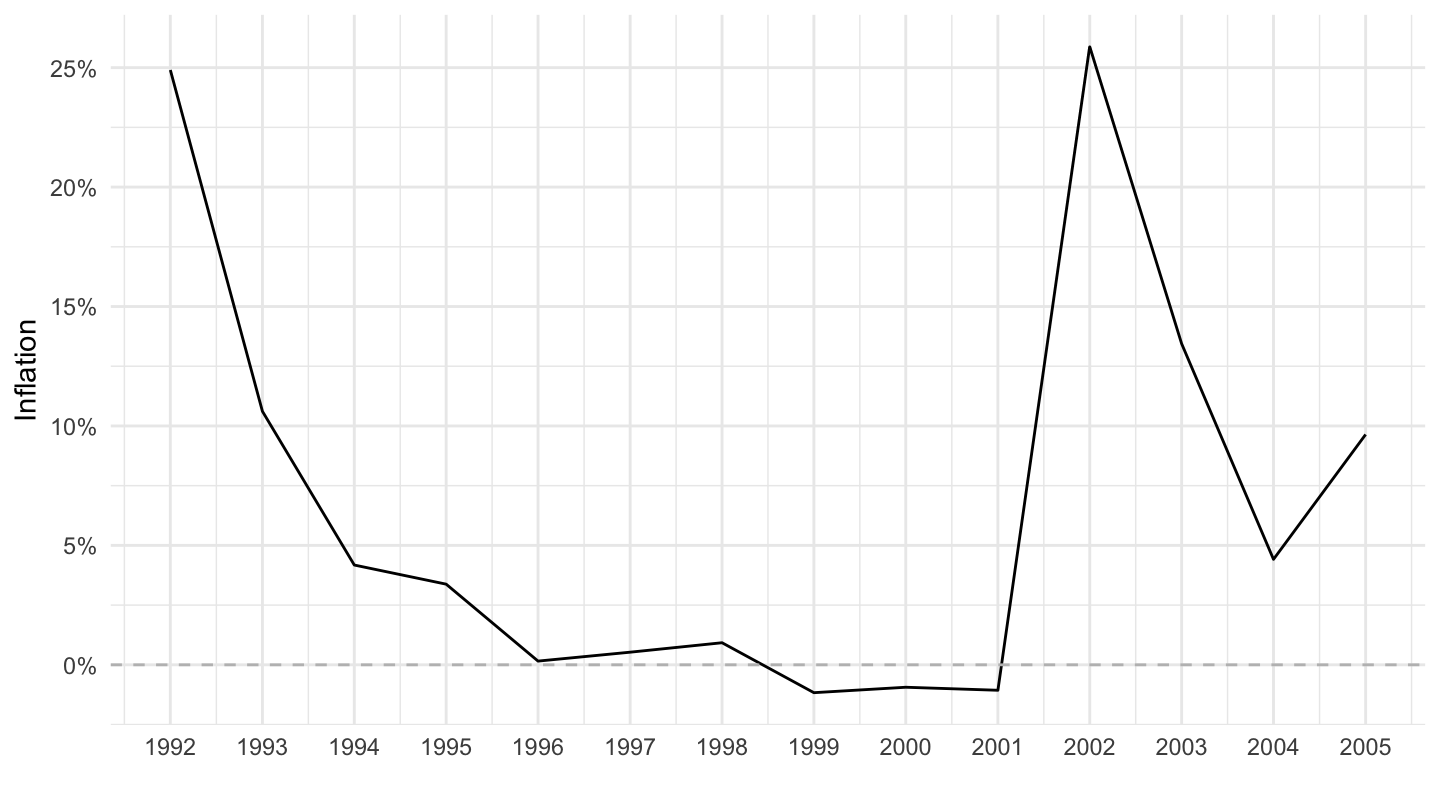
Japan
All
Code
CPI %>%
  filter(iso3c %in% c("JPN"),
         date >= as.Date("1952-01-01"),
         UNIT_MEASURE == 771,
         FREQ == "A") %>%
  ggplot(.) + geom_line() + theme_minimal() +
  aes(x = date, y = value/100) + xlab("") + ylab("Inflation") +
  scale_x_date(breaks = seq(1900, 2100, 5) %>% paste0("-01-01") %>% as.Date,
               labels = date_format("%Y")) +
  scale_y_continuous(breaks = 0.01*seq(-10, 200, 2),
                     labels = percent_format(a = 1)) +
  geom_hline(yintercept = 0, linetype = "dashed", color = "grey")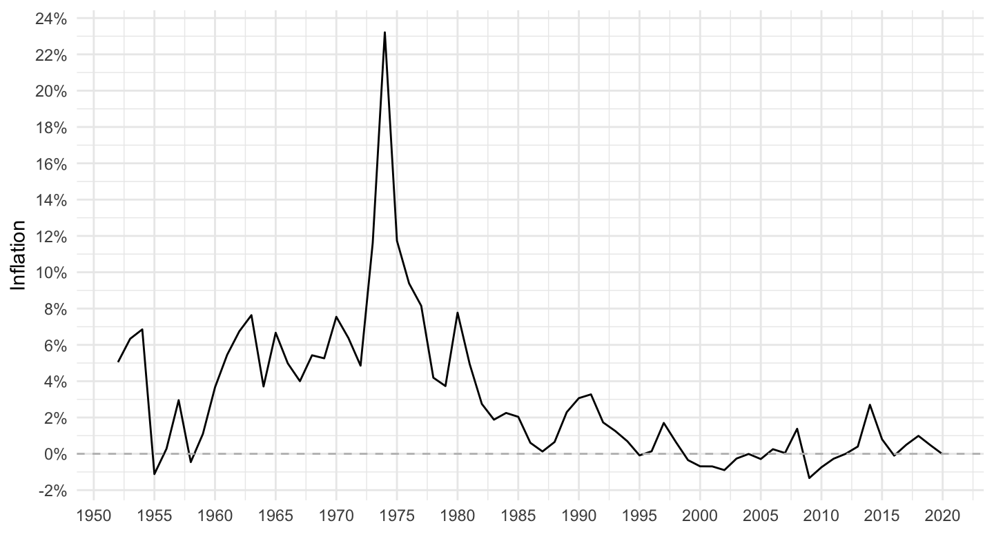
1952-
Code
CPI %>%
  filter(iso3c %in% c("JPN"),
         date >= as.Date("1952-01-01"),
         UNIT_MEASURE == 771,
         FREQ == "A") %>%
  ggplot(.) + geom_line() + theme_minimal() +
  aes(x = date, y = value/100) + xlab("") + ylab("Inflation") +
  scale_x_date(breaks = seq(1900, 2100, 5) %>% paste0("-01-01") %>% as.Date,
               labels = date_format("%Y")) +
  scale_y_continuous(breaks = 0.01*seq(-10, 200, 1),
                     labels = percent_format(a = 1)) +
  geom_hline(yintercept = 0, linetype = "dashed", color = "grey")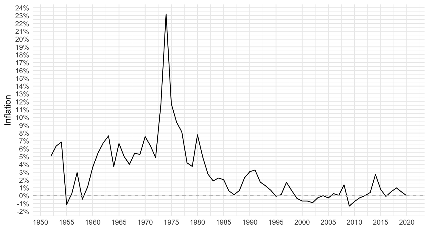
1980-
Code
CPI %>%
  filter(iso3c %in% c("JPN"),
         date >= as.Date("1980-01-01"),
         UNIT_MEASURE == 771,
         FREQ == "A") %>%
  ggplot(.) + geom_line() + theme_minimal() +
  aes(x = date, y = value/100) + xlab("") + ylab("Inflation") +
  scale_x_date(breaks = seq(1900, 2100, 2) %>% paste0("-01-01") %>% as.Date,
               labels = date_format("%Y")) +
  scale_y_continuous(breaks = 0.01*seq(-10, 200, 1),
                     labels = percent_format(a = 1)) +
  geom_hline(yintercept = 0, linetype = "dashed", color = "grey")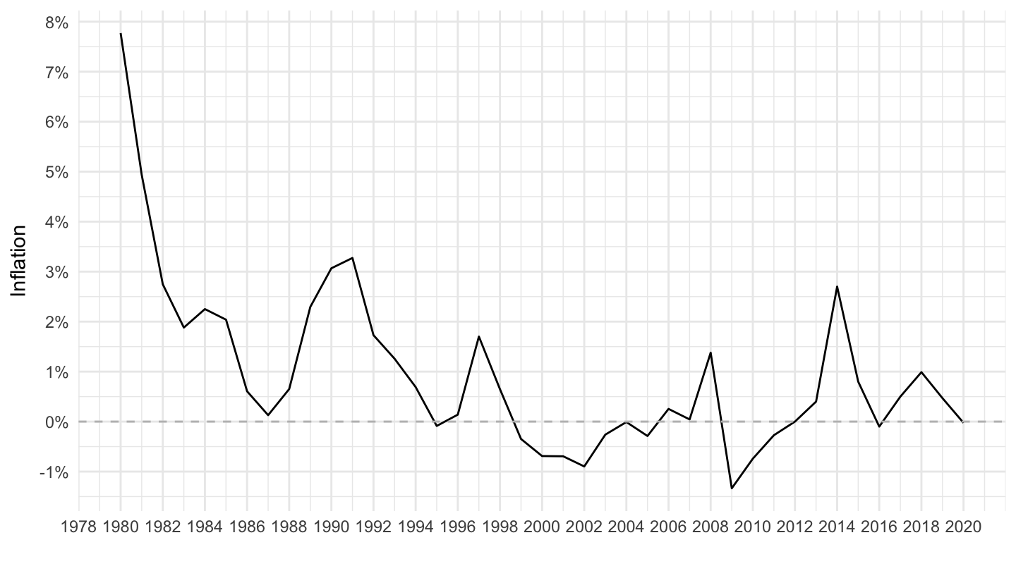
1986-
Code
CPI %>%
  filter(iso3c %in% c("JPN"),
         date >= as.Date("1986-01-01"),
         UNIT_MEASURE == 771,
         FREQ == "A") %>%
  ggplot(.) + geom_line() + theme_minimal() +
  aes(x = date, y = value/100) + xlab("") + ylab("Inflation") +
  scale_x_date(breaks = seq(1900, 2100, 2) %>% paste0("-01-01") %>% as.Date,
               labels = date_format("%Y")) +
  scale_y_continuous(breaks = 0.01*seq(-10, 200, 1),
                     labels = percent_format(a = 1)) +
  geom_hline(yintercept = 0, linetype = "dashed", color = "grey")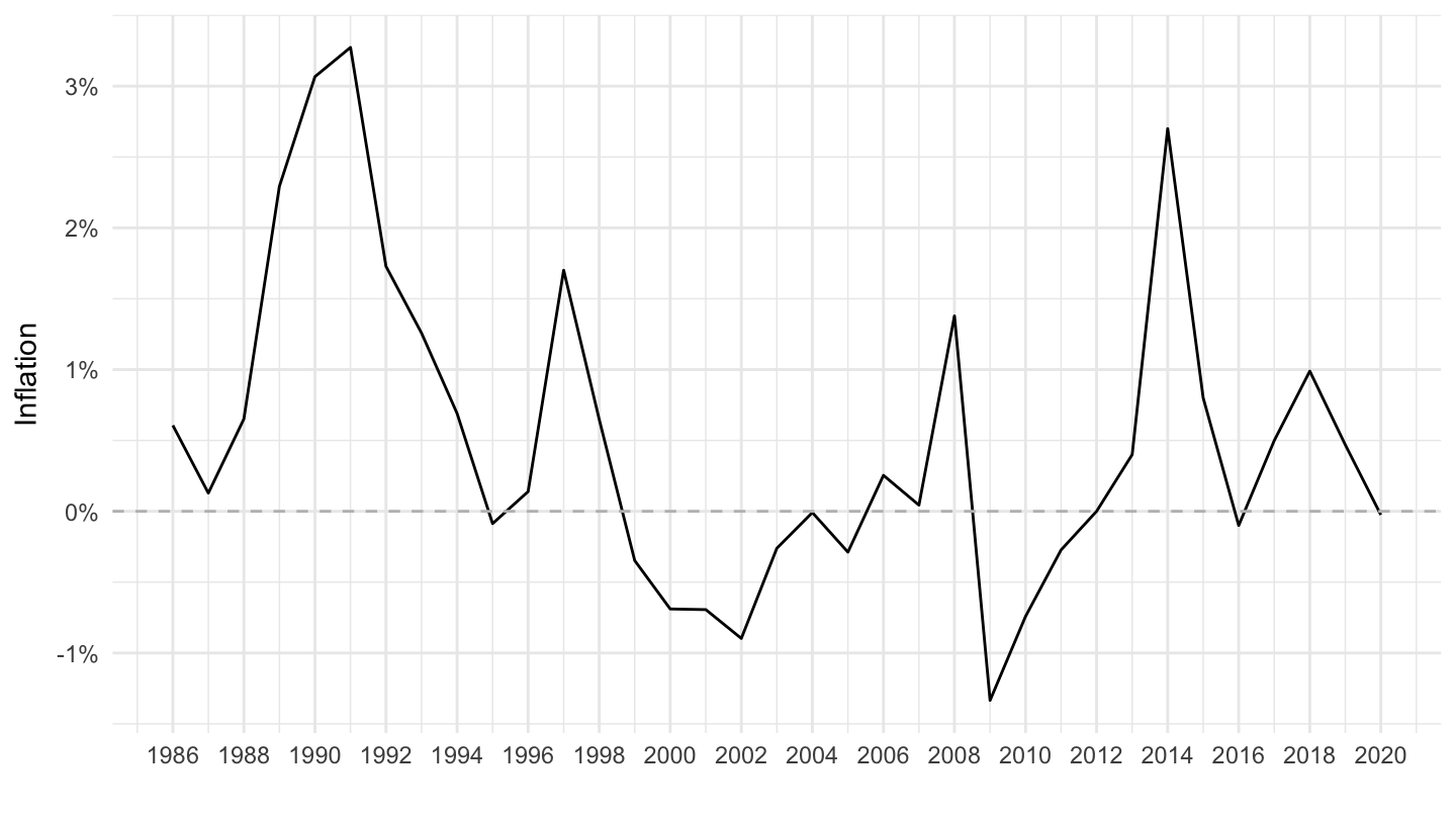
Italy
Code
CPI %>%
  filter(iso3c %in% c("ITA"),
         UNIT_MEASURE == 771,
         FREQ == "A") %>%
  ggplot(.) + geom_line() + theme_minimal() +
  aes(x = date, y = value/100) + xlab("") + ylab("Inflation") +
  scale_x_date(breaks = seq(1800, 2100, 10) %>% paste0("-01-01") %>% as.Date,
               labels = date_format("%Y")) +
  scale_y_continuous(breaks = 0.01*seq(-100, 200, 5),
                     labels = percent_format(a = 1)) +
  geom_hline(yintercept = 0, linetype = "dashed", color = "grey")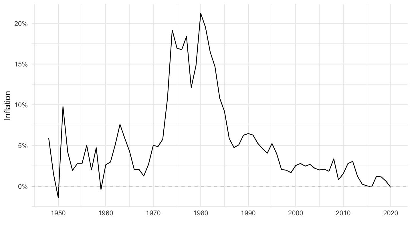
Italy (1952-)
Code
CPI %>%
  filter(iso3c %in% c("ITA"),
         date >= as.Date("1952-01-01"),
         UNIT_MEASURE == 771,
         FREQ == "A") %>%
  ggplot(.) + geom_line() + theme_minimal() +
  aes(x = date, y = value/100) + xlab("") + ylab("Inflation") +
  scale_x_date(breaks = seq(1900, 2100, 5) %>% paste0("-01-01") %>% as.Date,
               labels = date_format("%Y")) +
  scale_y_continuous(breaks = 0.01*seq(-10, 200, 2),
                     labels = percent_format(a = 1)) +
  geom_hline(yintercept = 0, linetype = "dashed", color = "grey")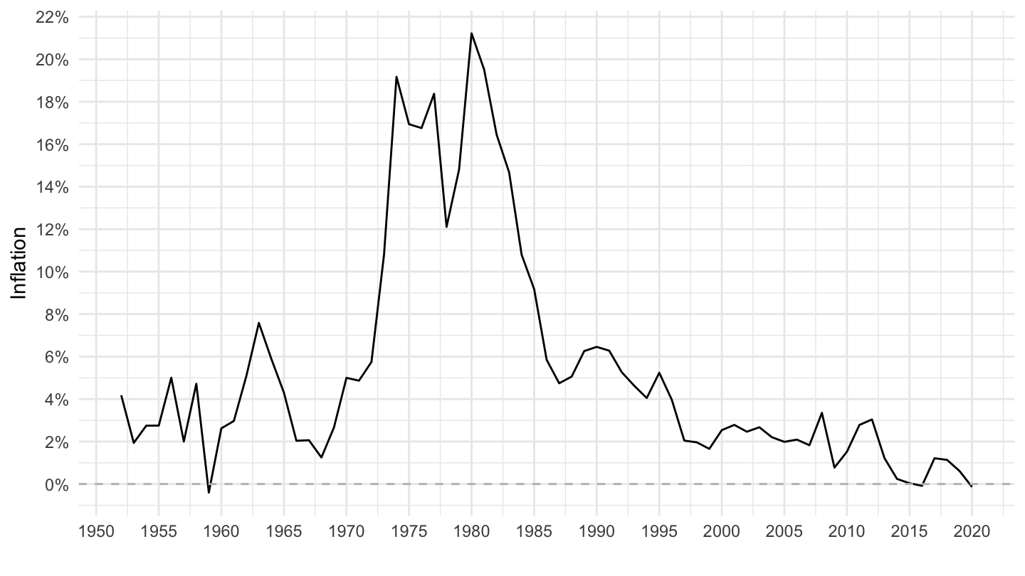
Germany
All
Code
CPI %>%
  filter(iso3c %in% c("DEU"),
         UNIT_MEASURE == 771,
         FREQ == "A") %>%
  ggplot(.) + geom_line() + theme_minimal() +
  aes(x = date, y = value/100) + xlab("") + ylab("Inflation") +
  scale_x_date(breaks = seq(1800, 2100, 10) %>% paste0("-01-01") %>% as.Date,
               labels = date_format("%Y")) +
  scale_y_continuous(breaks = 0.01*seq(-100, 200, 5),
                     labels = percent_format(a = 1)) +
  geom_hline(yintercept = 0, linetype = "dashed", color = "grey")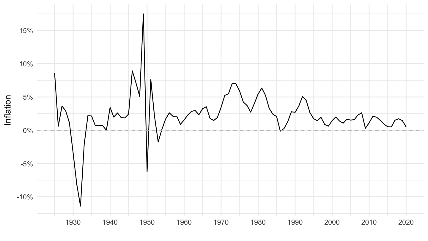
1952-1972
Code
CPI %>%
  filter(iso3c %in% c("DEU"),
         UNIT_MEASURE == 771,
         FREQ == "A",
         date >= as.Date("1952-01-01"),
         date <= as.Date("1972-01-01")) %>%
  ggplot(.) + geom_line() + theme_minimal() +
  aes(x = date, y = value/100) + xlab("") + ylab("Inflation") +
  scale_x_date(breaks = seq(1800, 2100, 2) %>% paste0("-01-01") %>% as.Date,
               labels = date_format("%Y")) +
  scale_y_continuous(breaks = 0.01*seq(-100, 200, 1),
                     labels = percent_format(a = 1)) +
  geom_hline(yintercept = 0, linetype = "dashed", color = "grey")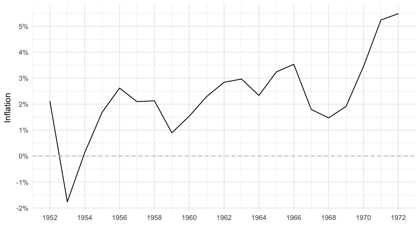
1952-1990
Code
CPI %>%
  filter(iso3c %in% c("DEU"),
         UNIT_MEASURE == 771,
         FREQ == "A",
         date >= as.Date("1952-01-01"),
         date <= as.Date("1990-01-01")) %>%
  ggplot(.) + geom_line() + theme_minimal() +
  aes(x = date, y = value/100) + xlab("") + ylab("Inflation") +
  scale_x_date(breaks = seq(1800, 2100, 5) %>% paste0("-01-01") %>% as.Date,
               labels = date_format("%Y")) +
  scale_y_continuous(breaks = 0.01*seq(-100, 200, 1),
                     labels = percent_format(a = 1)) +
  geom_hline(yintercept = 0, linetype = "dashed", color = "grey")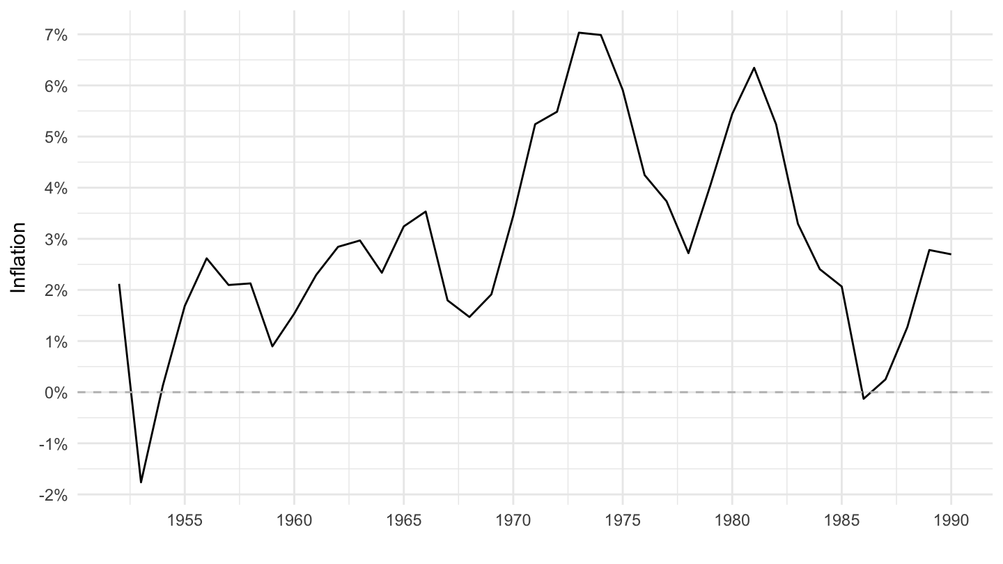
1952-
Code
CPI %>%
  filter(iso3c %in% c("DEU"),
         date >= as.Date("1952-01-01"),
         UNIT_MEASURE == 771,
         FREQ == "A") %>%
  ggplot(.) + geom_line() + theme_minimal() +
  aes(x = date, y = value/100) + xlab("") + ylab("Inflation") +
  scale_x_date(breaks = seq(1900, 2100, 5) %>% paste0("-01-01") %>% as.Date,
               labels = date_format("%Y")) +
  scale_y_continuous(breaks = 0.01*seq(-10, 200, 2),
                     labels = percent_format(a = 1)) +
  geom_hline(yintercept = 0, linetype = "dashed", color = "grey")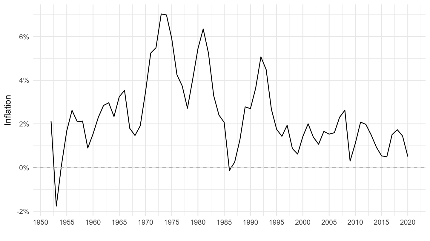
Austria
All
Code
CPI %>%
  filter(iso3c %in% c("AUT"),
         UNIT_MEASURE == 771,
         FREQ == "A") %>%
  ggplot(.) + geom_line() + theme_minimal() +
  aes(x = date, y = value/100) + xlab("") + ylab("Inflation") +
  scale_x_date(breaks = seq(1800, 2100, 10) %>% paste0("-01-01") %>% as.Date,
               labels = date_format("%Y")) +
  scale_y_continuous(breaks = 0.01*seq(-100, 200, 5),
                     labels = percent_format(a = 1)) +
  geom_hline(yintercept = 0, linetype = "dashed", color = "grey")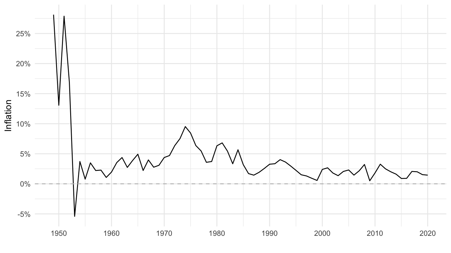
1952-
Code
CPI %>%
  filter(iso3c %in% c("AUT"),
         date >= as.Date("1952-01-01"),
         UNIT_MEASURE == 771,
         FREQ == "A") %>%
  ggplot(.) + geom_line() + theme_minimal() +
  aes(x = date, y = value/100) + xlab("") + ylab("Inflation") +
  scale_x_date(breaks = seq(1900, 2100, 5) %>% paste0("-01-01") %>% as.Date,
               labels = date_format("%Y")) +
  scale_y_continuous(breaks = 0.01*seq(-10, 200, 2),
                     labels = percent_format(a = 1)) +
  geom_hline(yintercept = 0, linetype = "dashed", color = "grey")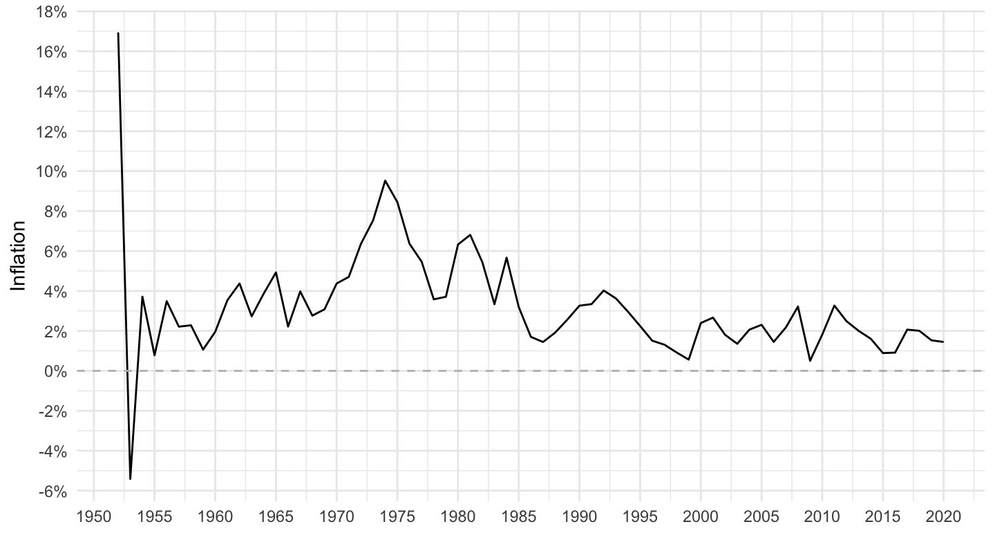
Luxembourg
Code
CPI %>%
  filter(iso3c %in% c("LUX"),
         UNIT_MEASURE == 771,
         FREQ == "A") %>%
  ggplot(.) + geom_line() + theme_minimal() +
  aes(x = date, y = value/100) + xlab("") + ylab("Inflation") +
  scale_x_date(breaks = seq(1800, 2100, 10) %>% paste0("-01-01") %>% as.Date,
               labels = date_format("%Y")) +
  scale_y_continuous(breaks = 0.01*seq(-100, 200, 2),
                     labels = percent_format(a = 1)) +
  geom_hline(yintercept = 0, linetype = "dashed", color = "grey")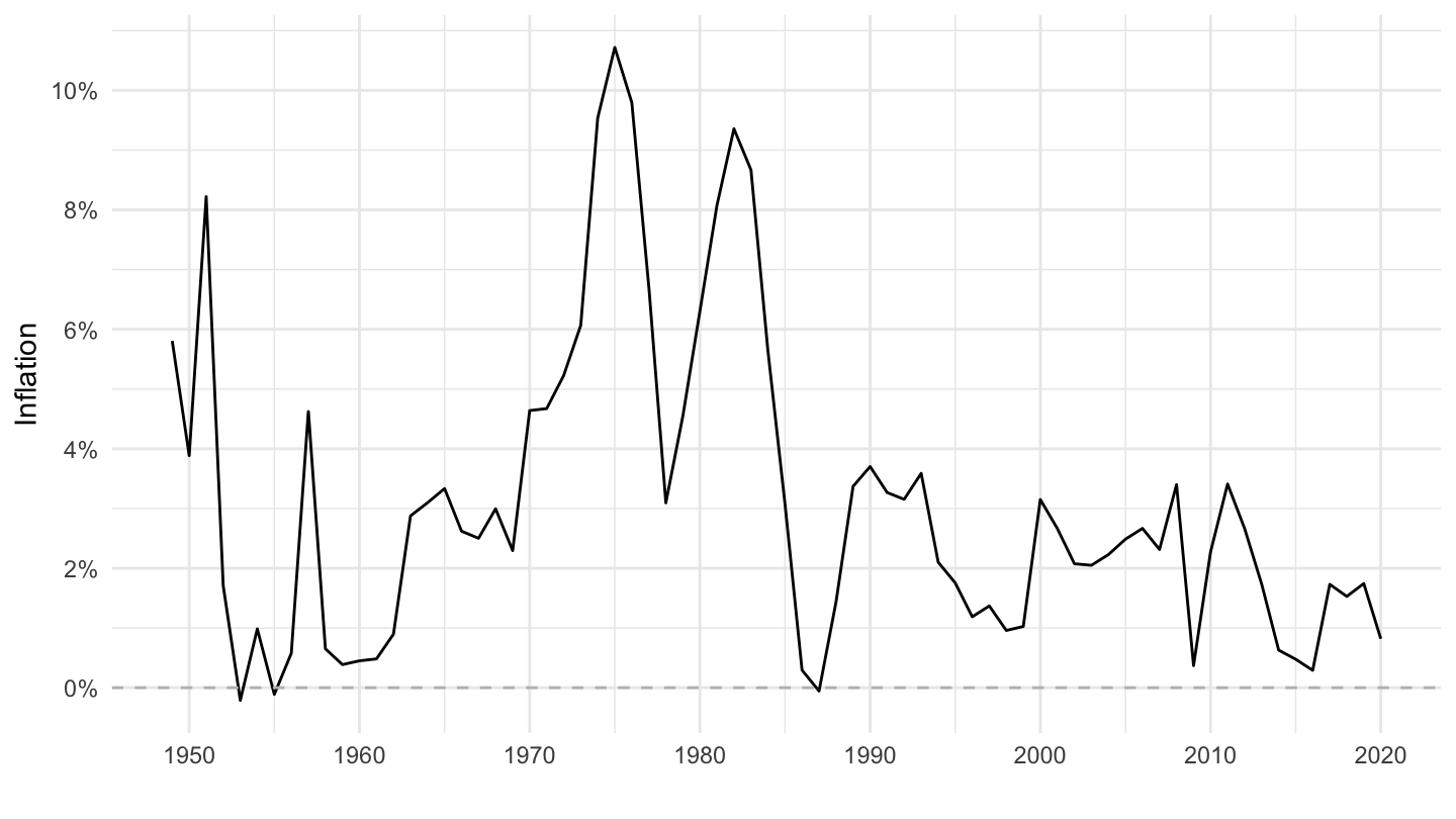
Luxembourg (1952-)
Code
CPI %>%
  filter(iso3c %in% c("LUX"),
         date >= as.Date("1952-01-01"),
         UNIT_MEASURE == 771,
         FREQ == "A") %>%
  ggplot(.) + geom_line() + theme_minimal() +
  aes(x = date, y = value/100) + xlab("") + ylab("Inflation") +
  scale_x_date(breaks = seq(1900, 2100, 5) %>% paste0("-01-01") %>% as.Date,
               labels = date_format("%Y")) +
  scale_y_continuous(breaks = 0.01*seq(-10, 200, 2),
                     labels = percent_format(a = 1)) +
  geom_hline(yintercept = 0, linetype = "dashed", color = "grey")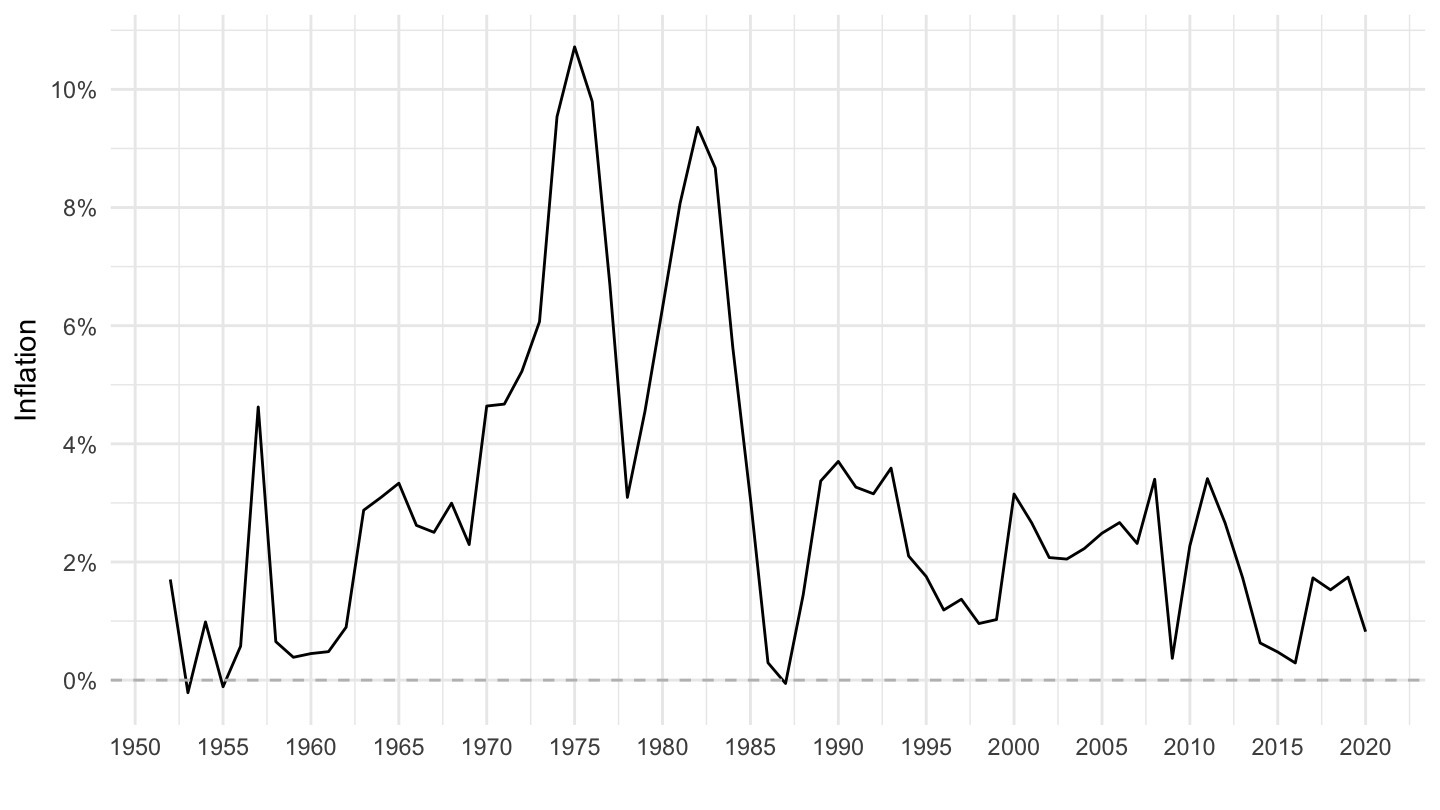
Portugal
Code
CPI %>%
  filter(iso3c %in% c("PRT"),
         UNIT_MEASURE == 771,
         FREQ == "A") %>%
  ggplot(.) + geom_line() + theme_minimal() +
  aes(x = date, y = value/100) + xlab("") + ylab("Inflation") +
  scale_x_date(breaks = seq(1900, 2100, 5) %>% paste0("-01-01") %>% as.Date,
               labels = date_format("%Y")) +
  scale_y_continuous(breaks = 0.01*seq(-10, 200, 2),
                     labels = percent_format(a = 1)) +
  geom_hline(yintercept = 0, linetype = "dashed", color = "grey")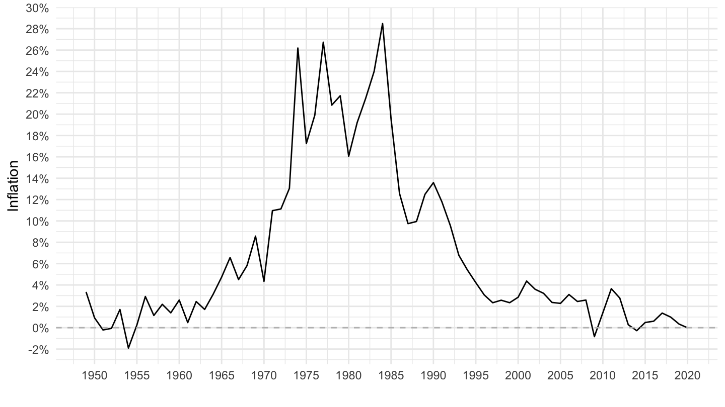
Peru
Code
CPI %>%
  filter(iso3c %in% c("PER"),
         UNIT_MEASURE == 771,
         FREQ == "A") %>%
  ggplot(.) + geom_line() + theme_minimal() +
  aes(x = date, y = value/100) + xlab("") + ylab("Inflation") +
  scale_x_date(breaks = seq(1900, 2100, 5) %>% paste0("-01-01") %>% as.Date,
               labels = date_format("%Y")) +
  scale_y_continuous(breaks = 0.01*seq(-1000, 10000, 1000),
                     labels = percent_format(a = 1)) +
  geom_hline(yintercept = 0, linetype = "dashed", color = "grey")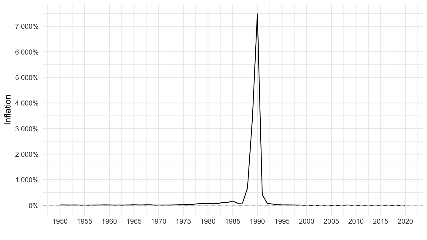
Hong Kong SAR
Code
CPI %>%
  filter(iso3c %in% c("HKG"),
         UNIT_MEASURE == 771,
         FREQ == "A") %>%
  ggplot(.) + geom_line() + theme_minimal() +
  aes(x = date, y = value/100) + xlab("") + ylab("Inflation") +
  scale_x_date(breaks = seq(1900, 2100, 5) %>% paste0("-01-01") %>% as.Date,
               labels = date_format("%Y")) +
  scale_y_continuous(breaks = 0.01*seq(-10, 200, 2),
                     labels = percent_format(a = 1)) +
  geom_hline(yintercept = 0, linetype = "dashed", color = "grey")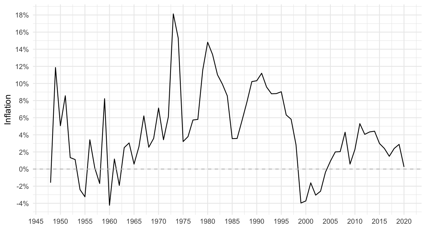
France
Code
CPI %>%
  filter(iso3c %in% c("FRA"),
         UNIT_MEASURE == 771,
         FREQ == "A") %>%
  ggplot(.) + geom_line() + theme_minimal() +
  aes(x = date, y = value/100) + xlab("") + ylab("Inflation") +
  scale_x_date(breaks = seq(1900, 2100, 5) %>% paste0("-01-01") %>% as.Date,
               labels = date_format("%Y")) +
  scale_y_continuous(breaks = 0.01*seq(-10, 200, 1),
                     labels = percent_format(a = 1)) +
  geom_hline(yintercept = 0, linetype = "dashed", color = "grey")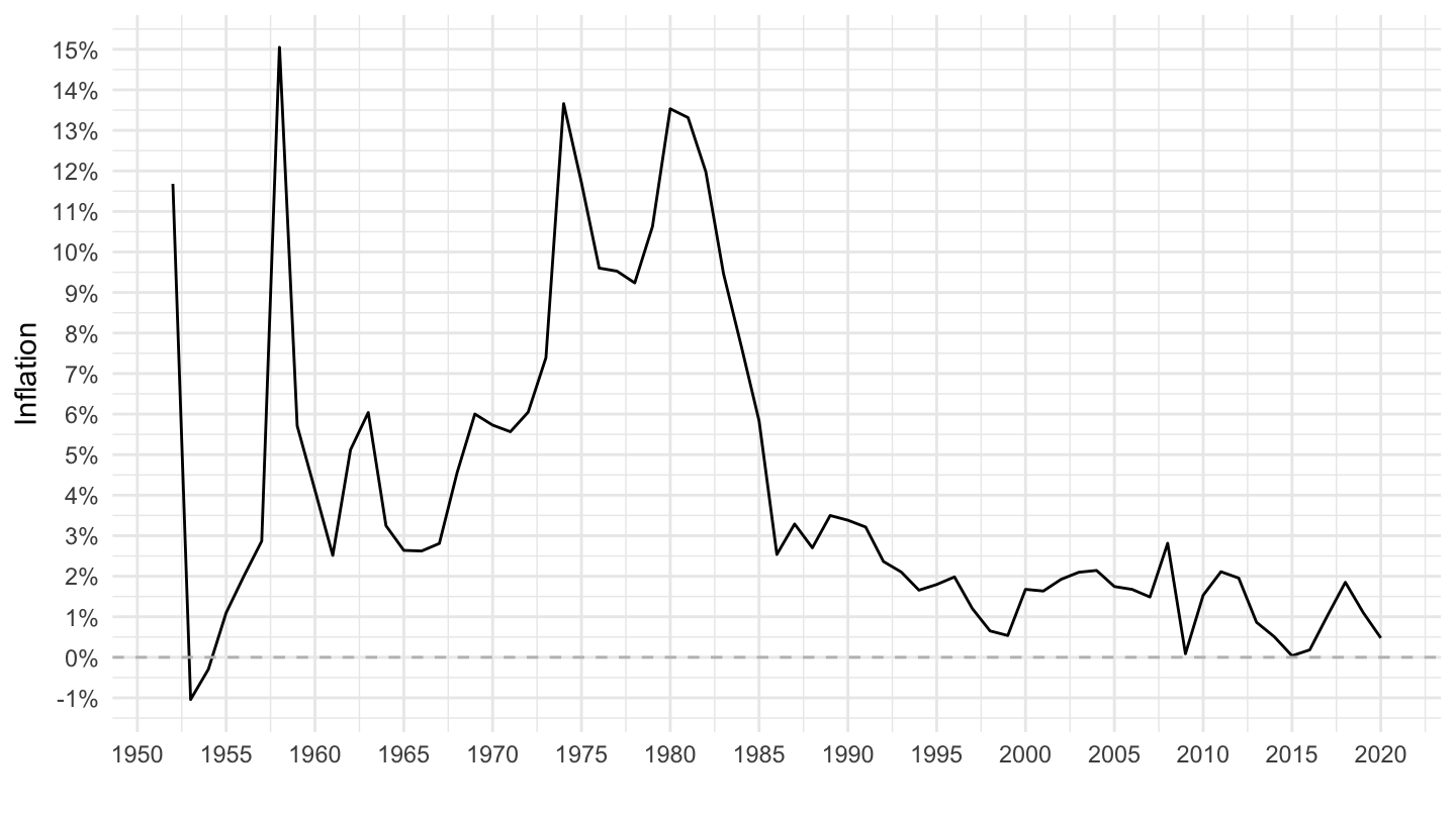
Israel
Code
CPI %>%
  filter(iso3c %in% c("ISR"),
         UNIT_MEASURE == 771,
         FREQ == "A") %>%
  ggplot(.) + geom_line() + theme_minimal() +
  aes(x = date, y = value/100) + xlab("") + ylab("Inflation") +
  scale_x_date(breaks = seq(1900, 2100, 5) %>% paste0("-01-01") %>% as.Date,
               labels = date_format("%Y")) +
  scale_y_continuous(breaks = 0.01*seq(-20, 700, 20),
                     labels = percent_format(a = 1)) +
  geom_hline(yintercept = 0, linetype = "dashed", color = "grey")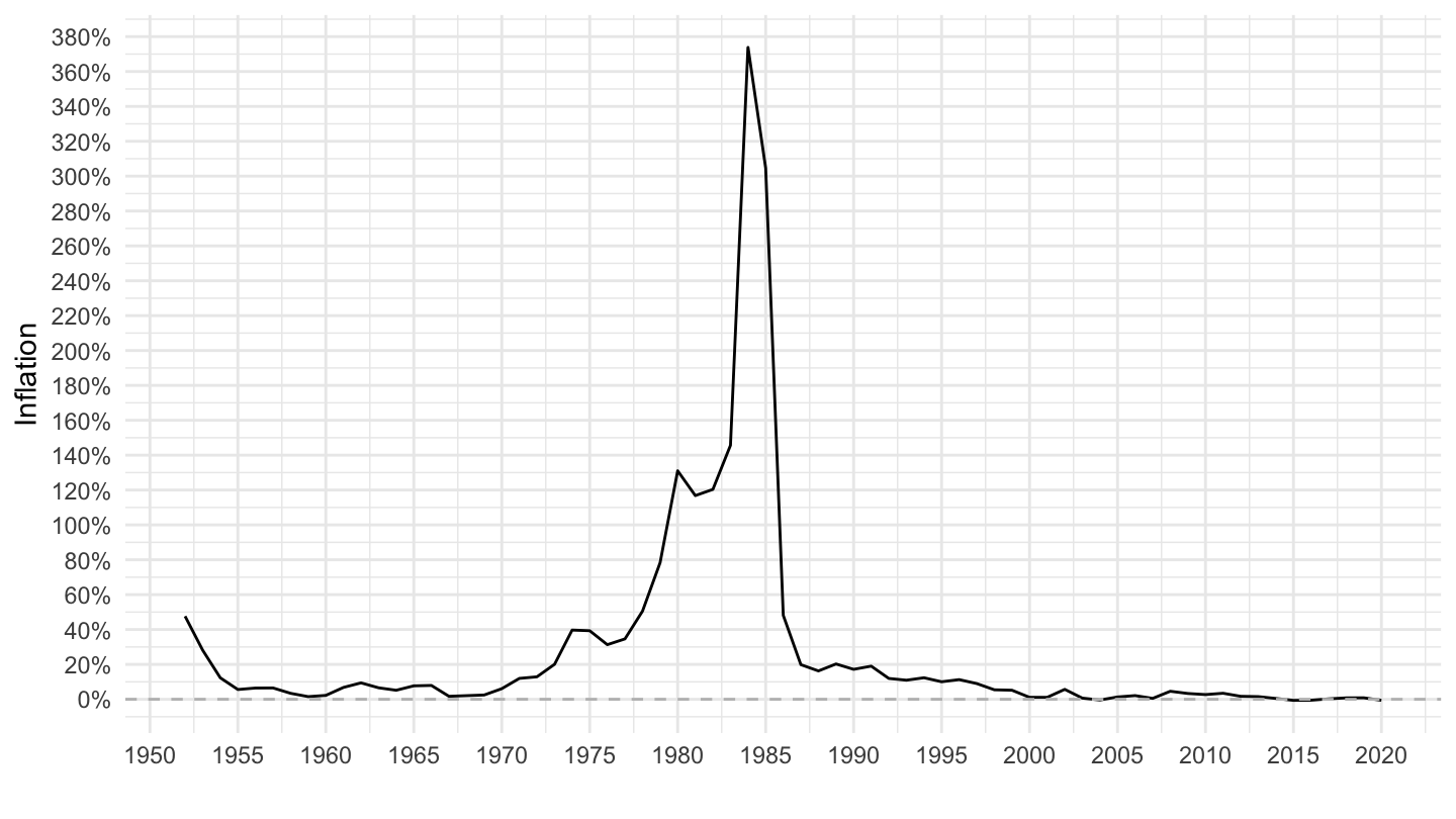
Finland
Code
CPI %>%
  filter(iso3c %in% c("FIN"),
         UNIT_MEASURE == 771,
         FREQ == "A") %>%
  ggplot(.) + geom_line() + theme_minimal() +
  aes(x = date, y = value/100) + xlab("") + ylab("Inflation") +
  scale_x_date(breaks = seq(1900, 2100, 5) %>% paste0("-01-01") %>% as.Date,
               labels = date_format("%Y")) +
  scale_y_continuous(breaks = 0.01*seq(-20, 700, 2),
                     labels = percent_format(a = 1)) +
  geom_hline(yintercept = 0, linetype = "dashed", color = "grey")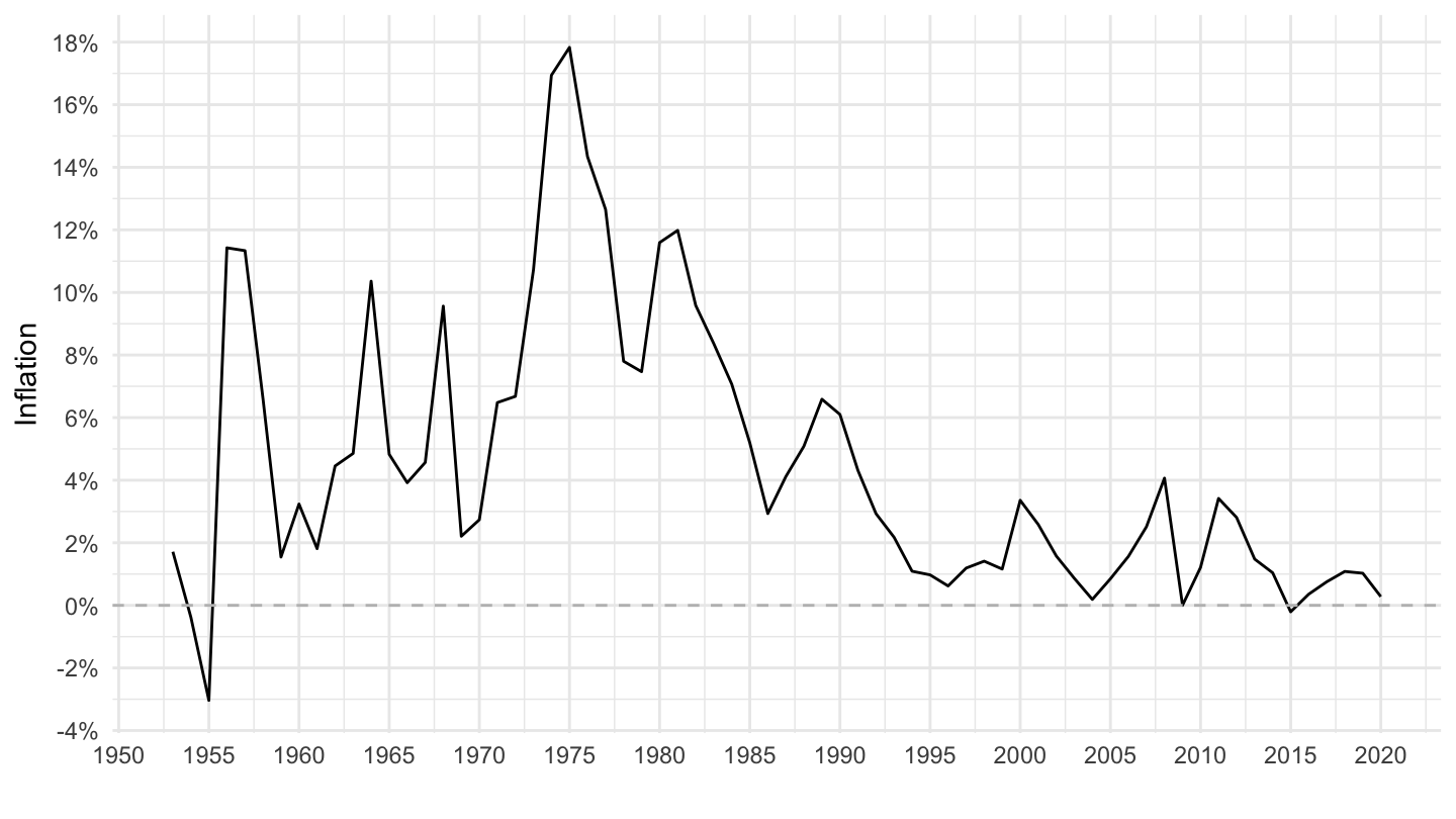
India
Code
CPI %>%
  filter(iso3c %in% c("IND"),
         UNIT_MEASURE == 771,
         FREQ == "A") %>%
  ggplot(.) + geom_line() + theme_minimal() +
  aes(x = date, y = value/100) + xlab("") + ylab("Inflation") +
  scale_x_date(breaks = seq(1900, 2100, 5) %>% paste0("-01-01") %>% as.Date,
               labels = date_format("%Y")) +
  scale_y_continuous(breaks = 0.01*seq(-20, 700, 2),
                     labels = percent_format(a = 1)) +
  geom_hline(yintercept = 0, linetype = "dashed", color = "grey")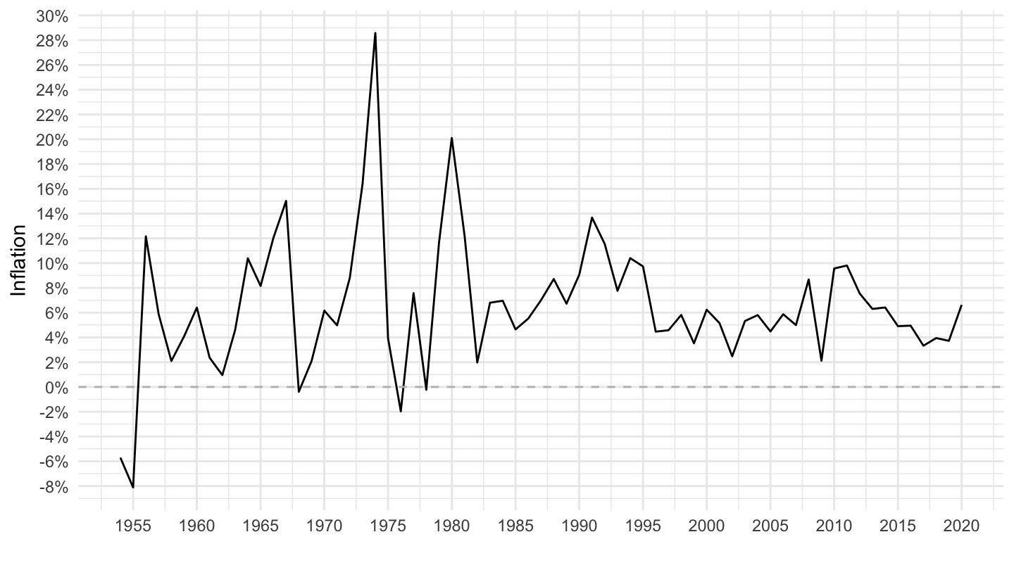
Spain
Code
CPI %>%
  filter(iso3c %in% c("ESP"),
         UNIT_MEASURE == 771,
         FREQ == "A") %>%
  ggplot(.) + geom_line() + theme_minimal() +
  aes(x = date, y = value/100) + xlab("") + ylab("Inflation") +
  scale_x_date(breaks = seq(1900, 2100, 5) %>% paste0("-01-01") %>% as.Date,
               labels = date_format("%Y")) +
  scale_y_continuous(breaks = 0.01*seq(-20, 700, 2),
                     labels = percent_format(a = 1)) +
  geom_hline(yintercept = 0, linetype = "dashed", color = "grey")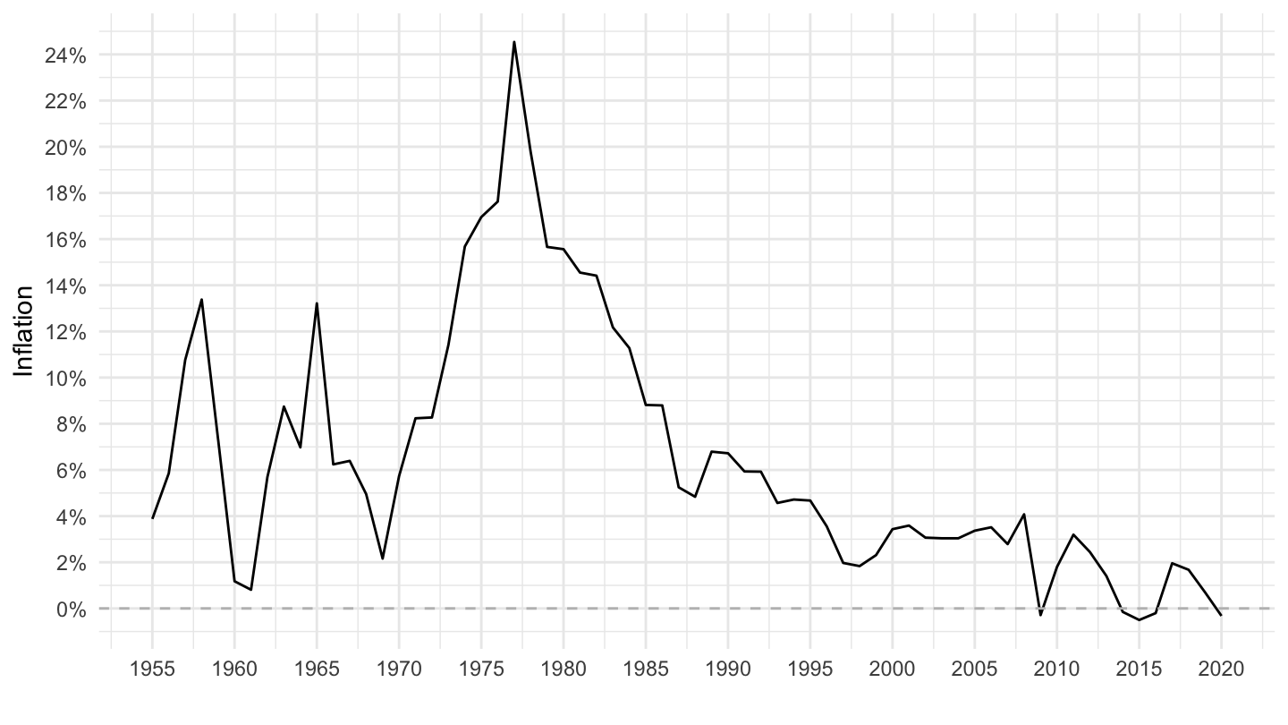
Philippines
Code
CPI %>%
  filter(iso3c %in% c("PHL"),
         UNIT_MEASURE == 771,
         FREQ == "A") %>%
  ggplot(.) + geom_line() + theme_minimal() +
  aes(x = date, y = value/100) + xlab("") + ylab("Inflation") +
  scale_x_date(breaks = seq(1900, 2100, 5) %>% paste0("-01-01") %>% as.Date,
               labels = date_format("%Y")) +
  scale_y_continuous(breaks = 0.01*seq(-20, 700, 2),
                     labels = percent_format(a = 1)) +
  geom_hline(yintercept = 0, linetype = "dashed", color = "grey")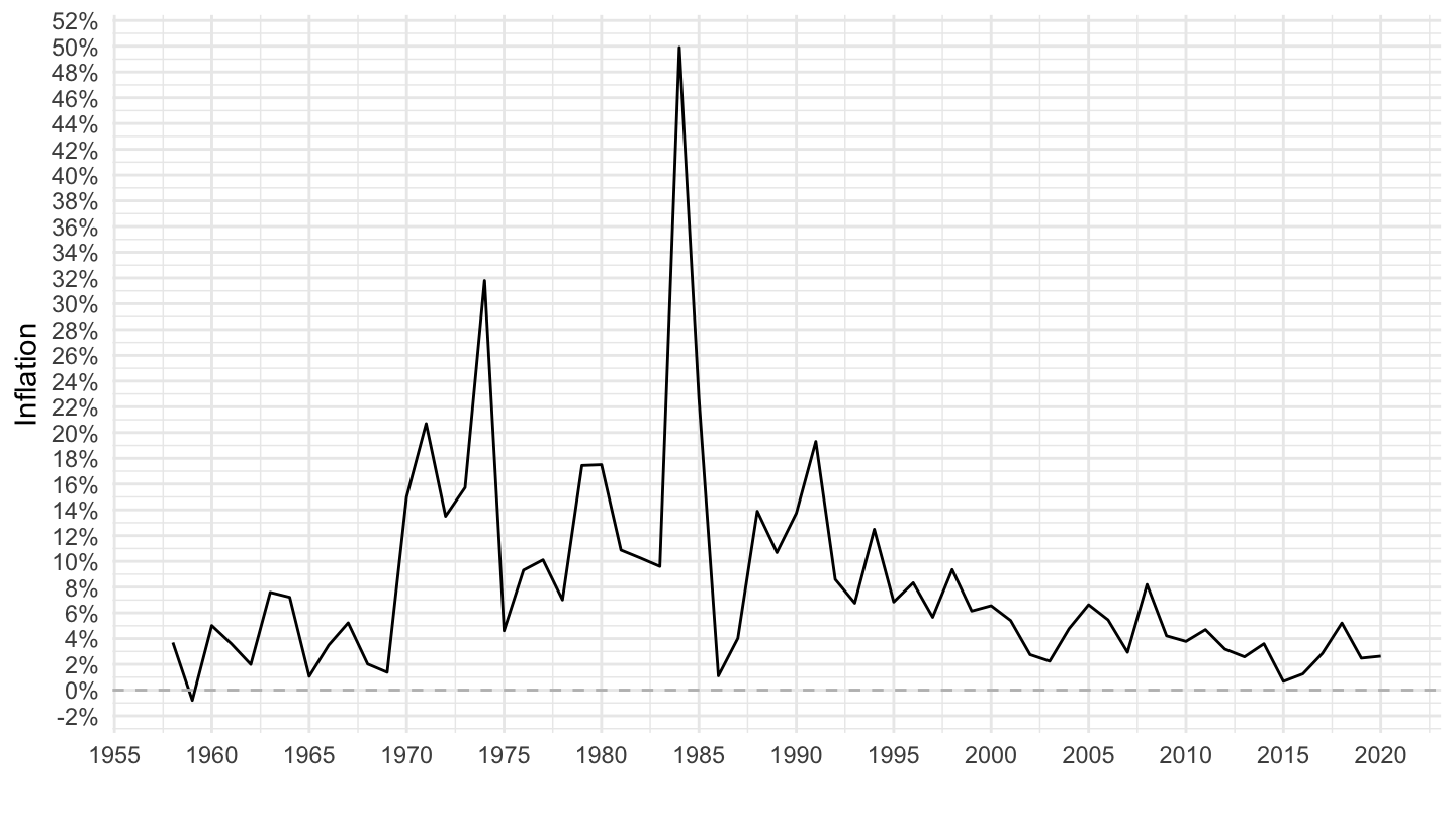
Greece
Code
CPI %>%
  filter(iso3c %in% c("GRC"),
         UNIT_MEASURE == 771,
         FREQ == "A") %>%
  ggplot(.) + geom_line() + theme_minimal() +
  aes(x = date, y = value/100) + xlab("") + ylab("Inflation") +
  scale_x_date(breaks = seq(1900, 2100, 5) %>% paste0("-01-01") %>% as.Date,
               labels = date_format("%Y")) +
  scale_y_continuous(breaks = 0.01*seq(-20, 700, 2),
                     labels = percent_format(a = 1)) +
  geom_hline(yintercept = 0, linetype = "dashed", color = "grey")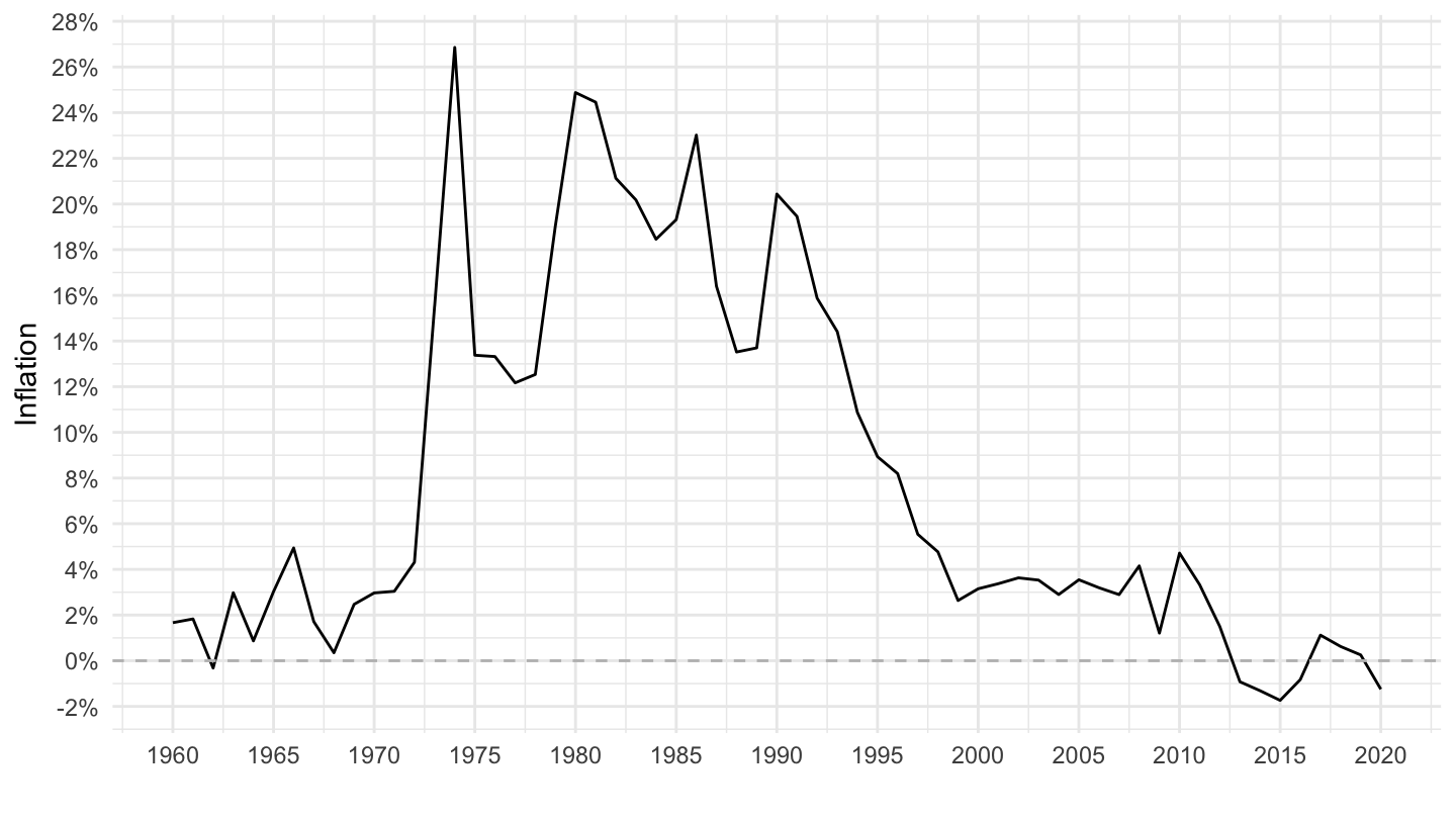
Netherlands
Code
CPI %>%
  filter(iso3c %in% c("NLD"),
         UNIT_MEASURE == 771,
         FREQ == "A") %>%
  ggplot(.) + geom_line() + theme_minimal() +
  aes(x = date, y = value/100) + xlab("") + ylab("Inflation") +
  scale_x_date(breaks = seq(1900, 2100, 5) %>% paste0("-01-01") %>% as.Date,
               labels = date_format("%Y")) +
  scale_y_continuous(breaks = 0.01*seq(-20, 700, 2),
                     labels = percent_format(a = 1)) +
  geom_hline(yintercept = 0, linetype = "dashed", color = "grey")
Netherlands (1952-)
Code
CPI %>%
  filter(iso3c %in% c("NLD"),
         date >= as.Date("1952-01-01"),
         UNIT_MEASURE == 771,
         FREQ == "A") %>%
  ggplot(.) + geom_line() + theme_minimal() +
  aes(x = date, y = value/100) + xlab("") + ylab("Inflation") +
  scale_x_date(breaks = seq(1900, 2100, 5) %>% paste0("-01-01") %>% as.Date,
               labels = date_format("%Y")) +
  scale_y_continuous(breaks = 0.01*seq(-20, 700, 2),
                     labels = percent_format(a = 1)) +
  geom_hline(yintercept = 0, linetype = "dashed", color = "grey")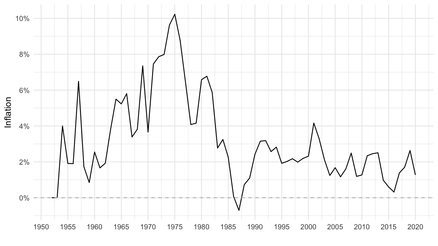
Singapore
Code
CPI %>%
  filter(iso3c %in% c("SGP"),
         UNIT_MEASURE == 771,
         FREQ == "A") %>%
  ggplot(.) + geom_line() + theme_minimal() +
  aes(x = date, y = value/100) + xlab("") + ylab("Inflation") +
  scale_x_date(breaks = seq(1900, 2100, 5) %>% paste0("-01-01") %>% as.Date,
               labels = date_format("%Y")) +
  scale_y_continuous(breaks = 0.01*seq(-20, 700, 2),
                     labels = percent_format(a = 1)) +
  geom_hline(yintercept = 0, linetype = "dashed", color = "grey")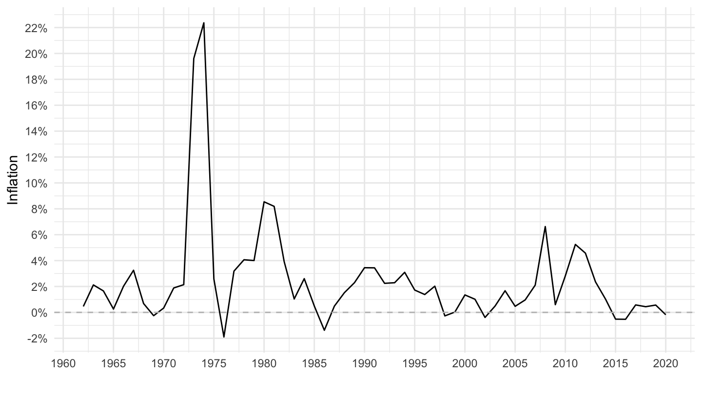
Turkey
Code
CPI %>%
  filter(iso3c %in% c("TUR"),
         UNIT_MEASURE == 771,
         FREQ == "A") %>%
  ggplot(.) + geom_line() + theme_minimal() +
  aes(x = date, y = value/100) + xlab("") + ylab("Inflation") +
  scale_x_date(breaks = seq(1900, 2100, 5) %>% paste0("-01-01") %>% as.Date,
               labels = date_format("%Y")) +
  scale_y_continuous(breaks = 0.01*seq(-20, 700, 10),
                     labels = percent_format(a = 1)) +
  geom_hline(yintercept = 0, linetype = "dashed", color = "grey")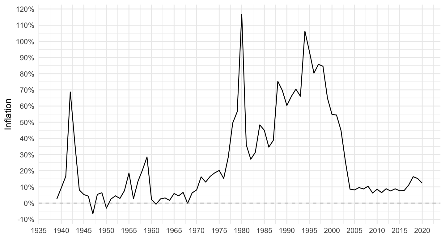
Korea
All
Code
CPI %>%
  filter(iso3c %in% c("KOR"),
         UNIT_MEASURE == 771,
         FREQ == "A") %>%
  ggplot(.) + geom_line() + theme_minimal() +
  aes(x = date, y = value/100) + xlab("") + ylab("Inflation") +
  scale_x_date(breaks = seq(1900, 2025, 5) %>% paste0("-01-01") %>% as.Date,
               labels = date_format("%Y")) +
  scale_y_continuous(breaks = 0.01*seq(-20, 700, 10),
                     labels = percent_format(a = 1)) +
  geom_hline(yintercept = 0, linetype = "dashed", color = "grey")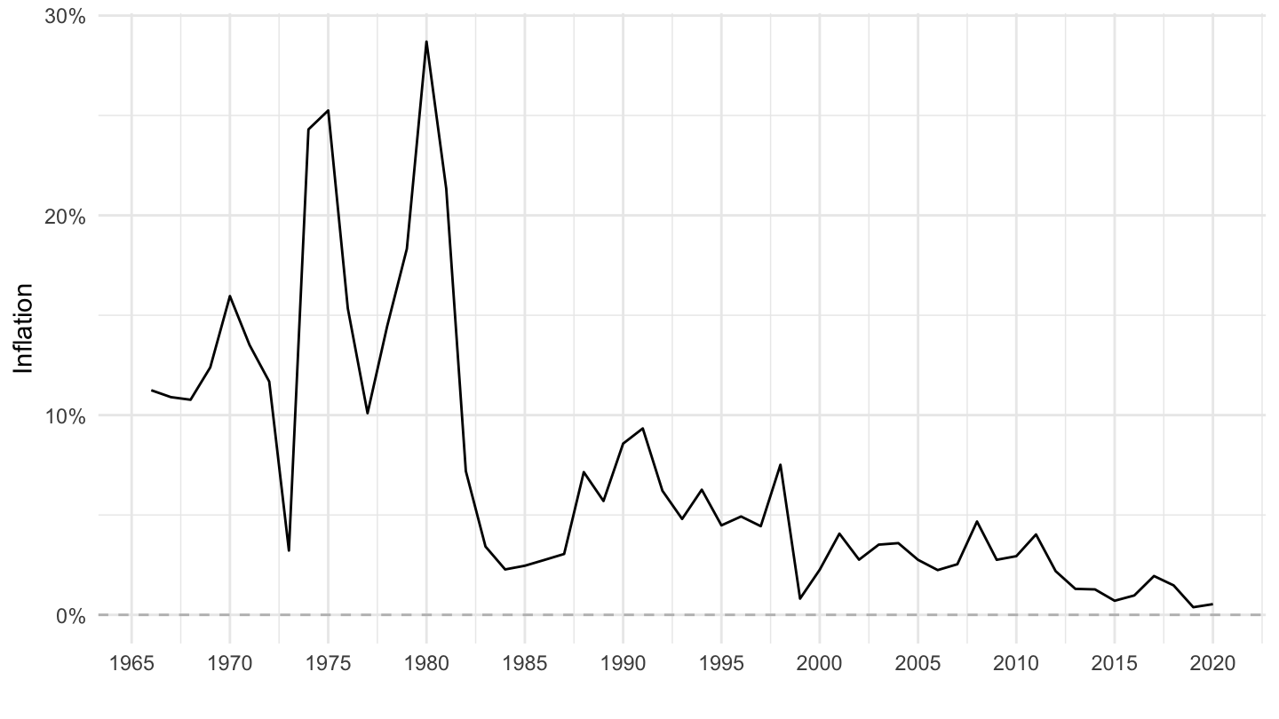
1990-
Code
CPI %>%
  filter(iso3c %in% c("KOR"),
         UNIT_MEASURE == 771,
         FREQ == "A") %>%
  filter(date >= as.Date("1990-01-01")) %>%
  ggplot(.) + geom_line() + theme_minimal() +
  aes(x = date, y = value/100) + xlab("") + ylab("Inflation") +
  scale_x_date(breaks = seq(1900, 2025, 2) %>% paste0("-01-01") %>% as.Date,
               labels = date_format("%Y")) +
  scale_y_continuous(breaks = 0.01*seq(-20, 700, 10),
                     labels = percent_format(a = 1)) +
  geom_hline(yintercept = 0, linetype = "dashed", color = "grey")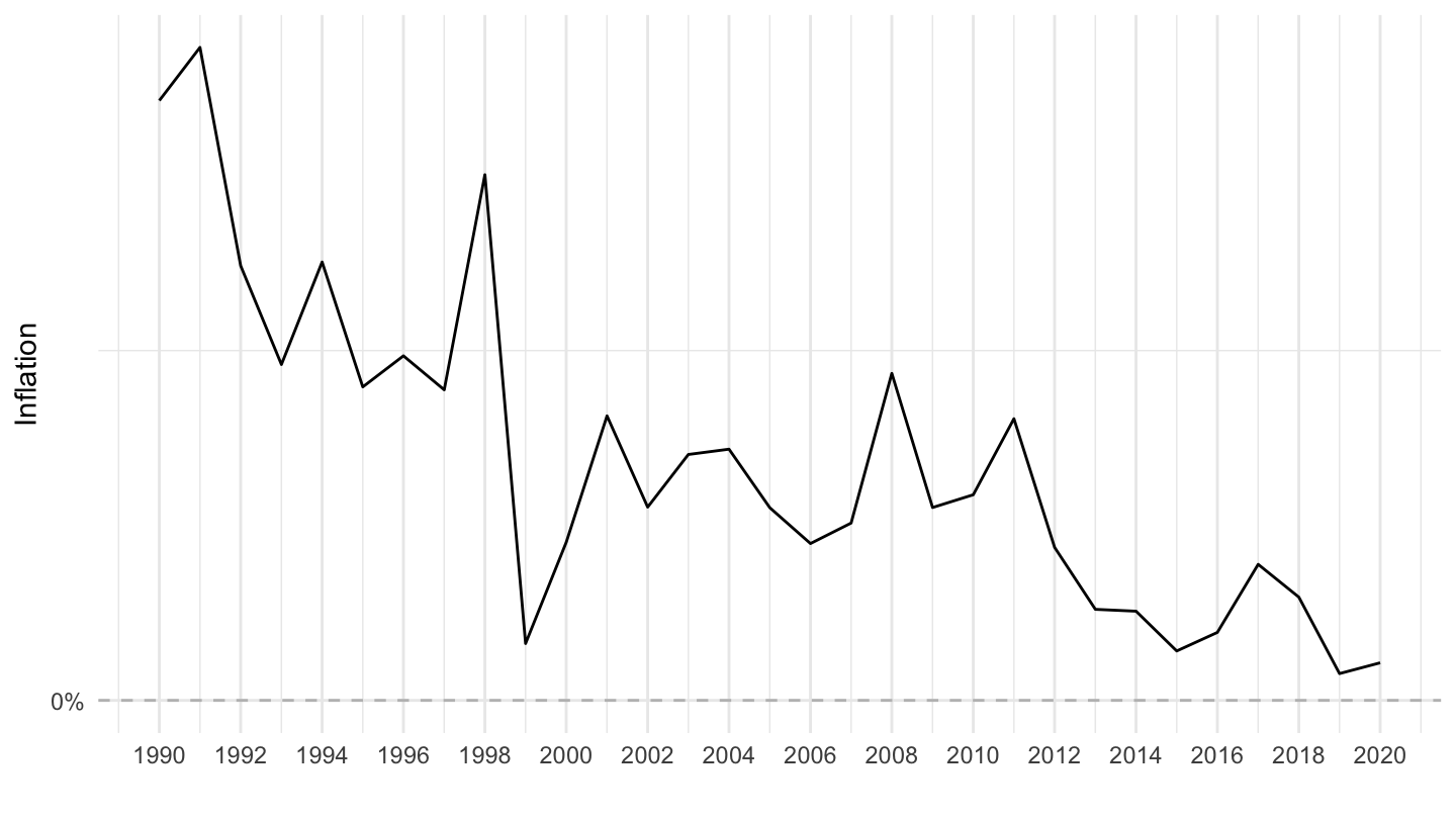
Mexico
Code
CPI %>%
  filter(iso3c %in% c("MEX"),
         UNIT_MEASURE == 771,
         FREQ == "A") %>%
  ggplot(.) + geom_line() + theme_minimal() +
  aes(x = date, y = value/100) + xlab("") + ylab("Inflation") +
  scale_x_date(breaks = seq(1900, 2100, 5) %>% paste0("-01-01") %>% as.Date,
               labels = date_format("%Y")) +
  scale_y_continuous(breaks = 0.01*seq(-20, 700, 10),
                     labels = percent_format(a = 1)) +
  geom_hline(yintercept = 0, linetype = "dashed", color = "grey")
Malaysia
Code
CPI %>%
  filter(iso3c %in% c("MYS"),
         UNIT_MEASURE == 771,
         FREQ == "A") %>%
  ggplot(.) + geom_line() + theme_minimal() +
  aes(x = date, y = value/100) + xlab("") + ylab("Inflation") +
  scale_x_date(breaks = seq(1900, 2100, 5) %>% paste0("-01-01") %>% as.Date,
               labels = date_format("%Y")) +
  scale_y_continuous(breaks = 0.01*seq(-20, 700, 2),
                     labels = percent_format(a = 1)) +
  geom_hline(yintercept = 0, linetype = "dashed", color = "grey")
Malta
Code
CPI %>%
  filter(iso3c %in% c("MLT"),
         UNIT_MEASURE == 771,
         FREQ == "A") %>%
  ggplot(.) + geom_line() + theme_minimal() +
  aes(x = date, y = value/100) + xlab("") + ylab("Inflation") +
  scale_x_date(breaks = seq(1900, 2100, 5) %>% paste0("-01-01") %>% as.Date,
               labels = date_format("%Y")) +
  scale_y_continuous(breaks = 0.01*seq(-20, 700, 2),
                     labels = percent_format(a = 1)) +
  geom_hline(yintercept = 0, linetype = "dashed", color = "grey")
Thailand
Code
CPI %>%
  filter(iso3c %in% c("THA"),
         UNIT_MEASURE == 771,
         FREQ == "A") %>%
  ggplot(.) + geom_line() + theme_minimal() +
  aes(x = date, y = value/100) + xlab("") + ylab("Inflation") +
  scale_x_date(breaks = seq(1900, 2100, 5) %>% paste0("-01-01") %>% as.Date,
               labels = date_format("%Y")) +
  scale_y_continuous(breaks = 0.01*seq(-20, 700, 2),
                     labels = percent_format(a = 1)) +
  geom_hline(yintercept = 0, linetype = "dashed", color = "grey")
Indonesia
Code
CPI %>%
  filter(iso3c %in% c("IDN"),
         UNIT_MEASURE == 771,
         FREQ == "A") %>%
  ggplot(.) + geom_line() + theme_minimal() +
  aes(x = date, y = value/100) + xlab("") + ylab("Inflation") +
  scale_x_date(breaks = seq(1900, 2100, 5) %>% paste0("-01-01") %>% as.Date,
               labels = date_format("%Y")) +
  scale_y_continuous(breaks = 0.01*seq(-20, 700, 5),
                     labels = percent_format(a = 1)) +
  geom_hline(yintercept = 0, linetype = "dashed", color = "grey")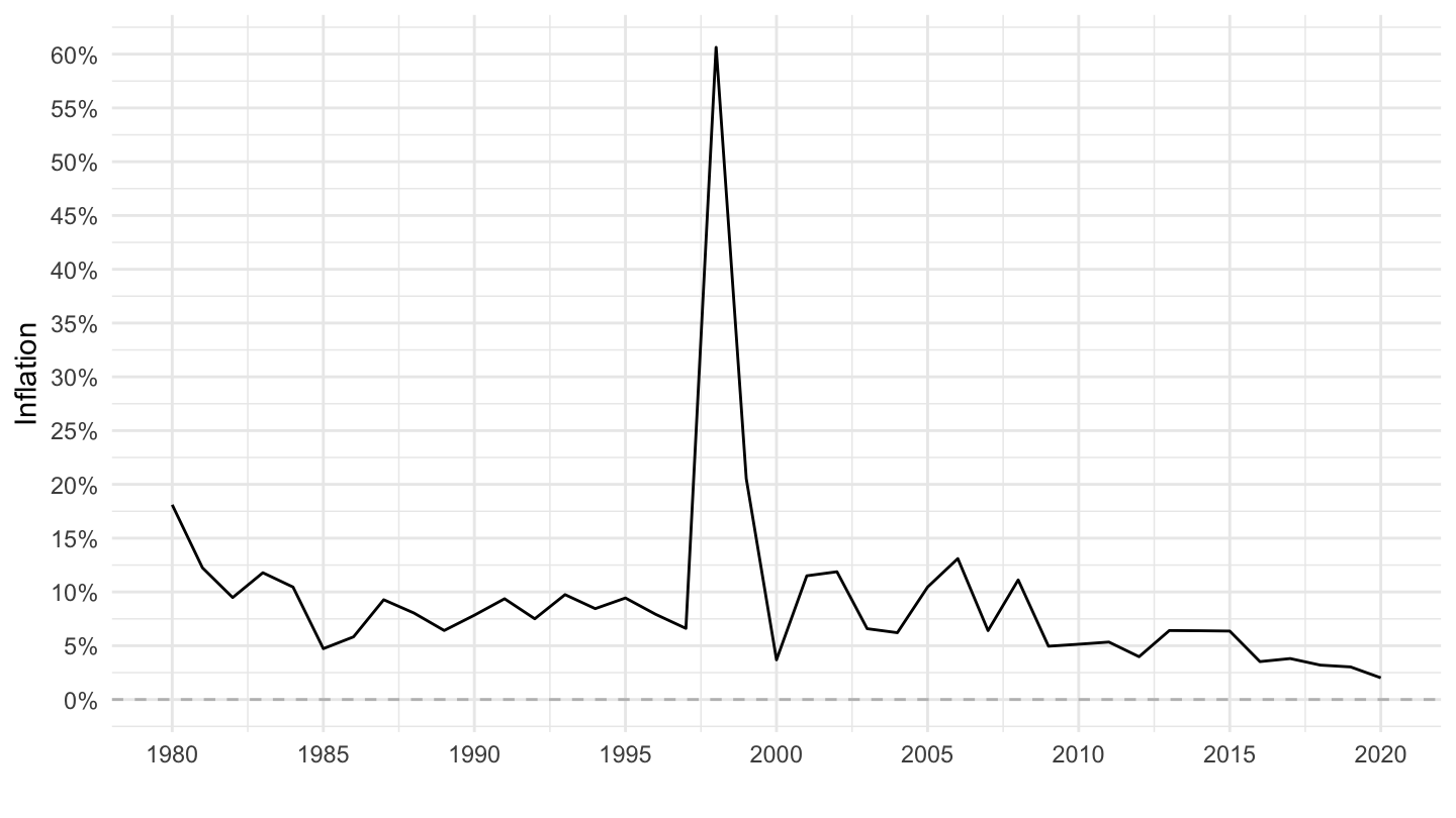
Brazil
Code
CPI %>%
  filter(iso3c %in% c("BRA"),
         UNIT_MEASURE == 771,
         FREQ == "A") %>%
  ggplot(.) + geom_line() + theme_minimal() +
  aes(x = date, y = value/100) + xlab("") + ylab("Inflation") +
  scale_x_date(breaks = seq(1900, 2100, 5) %>% paste0("-01-01") %>% as.Date,
               labels = date_format("%Y")) +
  scale_y_continuous(breaks = 0.01*seq(-100, 10000, 100),
                     labels = percent_format(a = 1)) +
  geom_hline(yintercept = 0, linetype = "dashed", color = "grey")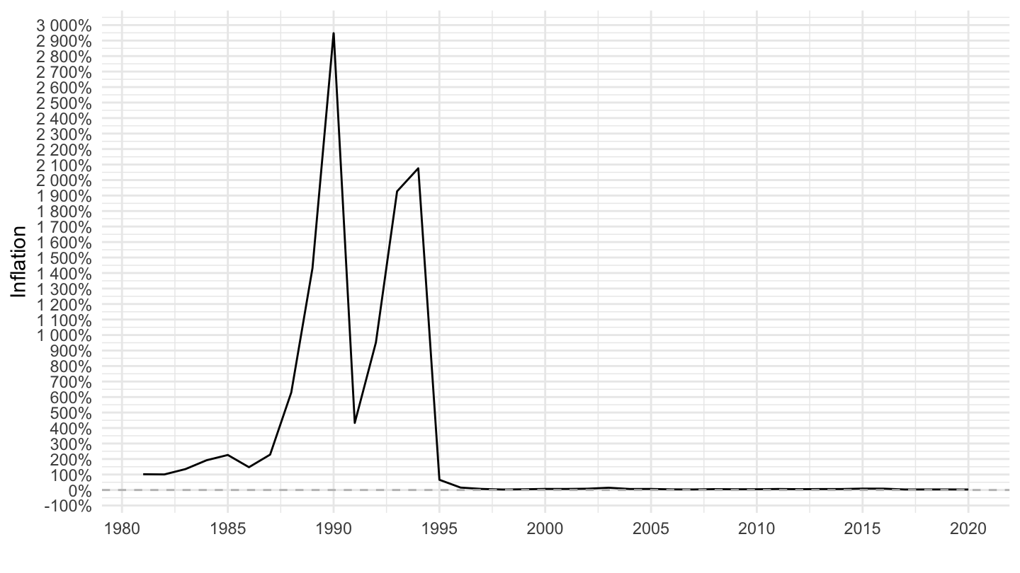
Cyprus
Code
CPI %>%
  filter(iso3c %in% c("CYP"),
         UNIT_MEASURE == 771,
         FREQ == "A") %>%
  ggplot(.) + geom_line() + theme_minimal() +
  aes(x = date, y = value/100) + xlab("") + ylab("Inflation") +
  scale_x_date(breaks = seq(1900, 2100, 5) %>% paste0("-01-01") %>% as.Date,
               labels = date_format("%Y")) +
  scale_y_continuous(breaks = 0.01*seq(-100, 10000, 2),
                     labels = percent_format(a = 1)) +
  geom_hline(yintercept = 0, linetype = "dashed", color = "grey")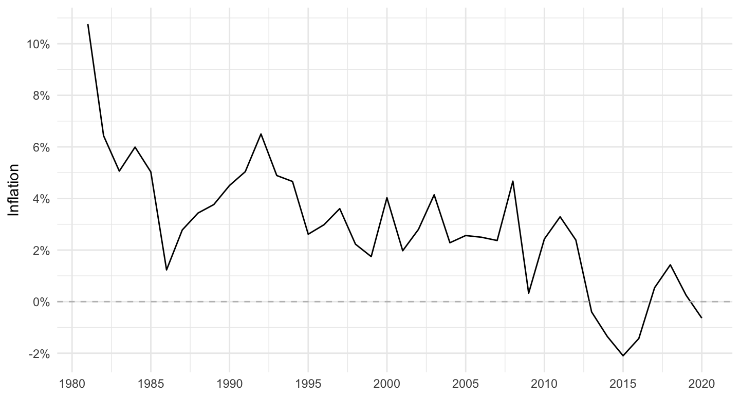
Poland
Code
CPI %>%
  filter(iso3c %in% c("POL"),
         UNIT_MEASURE == 771,
         FREQ == "A") %>%
  ggplot(.) + geom_line() + theme_minimal() +
  aes(x = date, y = value/100) + xlab("") + ylab("Inflation") +
  scale_x_date(breaks = seq(1900, 2100, 5) %>% paste0("-01-01") %>% as.Date,
               labels = date_format("%Y")) +
  scale_y_continuous(breaks = 0.01*seq(-100, 10000, 100),
                     labels = percent_format(a = 1)) +
  geom_hline(yintercept = 0, linetype = "dashed", color = "grey")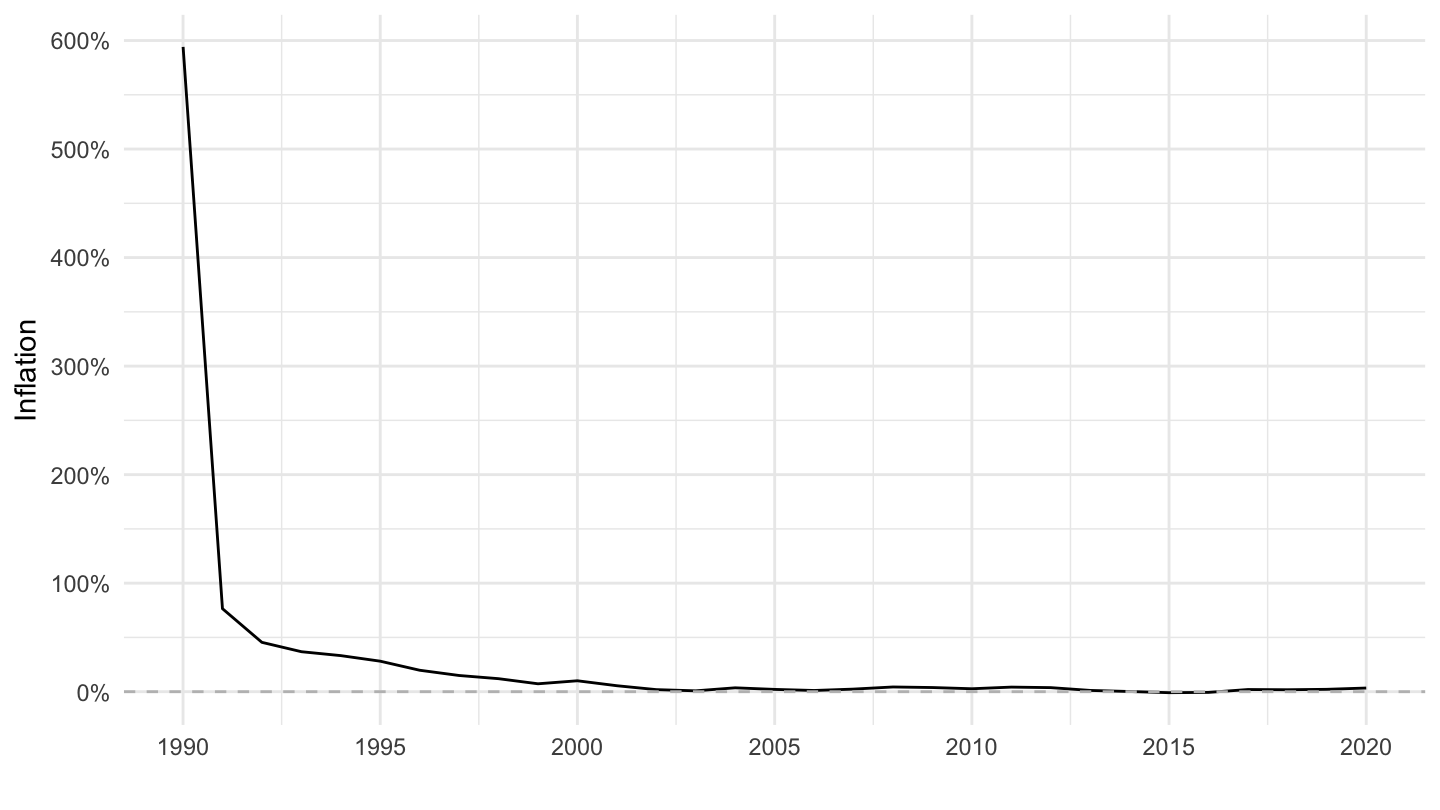
Czech Republic
Code
CPI %>%
  filter(iso3c %in% c("CZE"),
         UNIT_MEASURE == 771,
         FREQ == "A") %>%
  ggplot(.) + geom_line() + theme_minimal() +
  aes(x = date, y = value/100) + xlab("") + ylab("Inflation") +
  scale_x_date(breaks = seq(1900, 2100, 5) %>% paste0("-01-01") %>% as.Date,
               labels = date_format("%Y")) +
  scale_y_continuous(breaks = 0.01*seq(-100, 10000, 10),
                     labels = percent_format(a = 1)) +
  geom_hline(yintercept = 0, linetype = "dashed", color = "grey")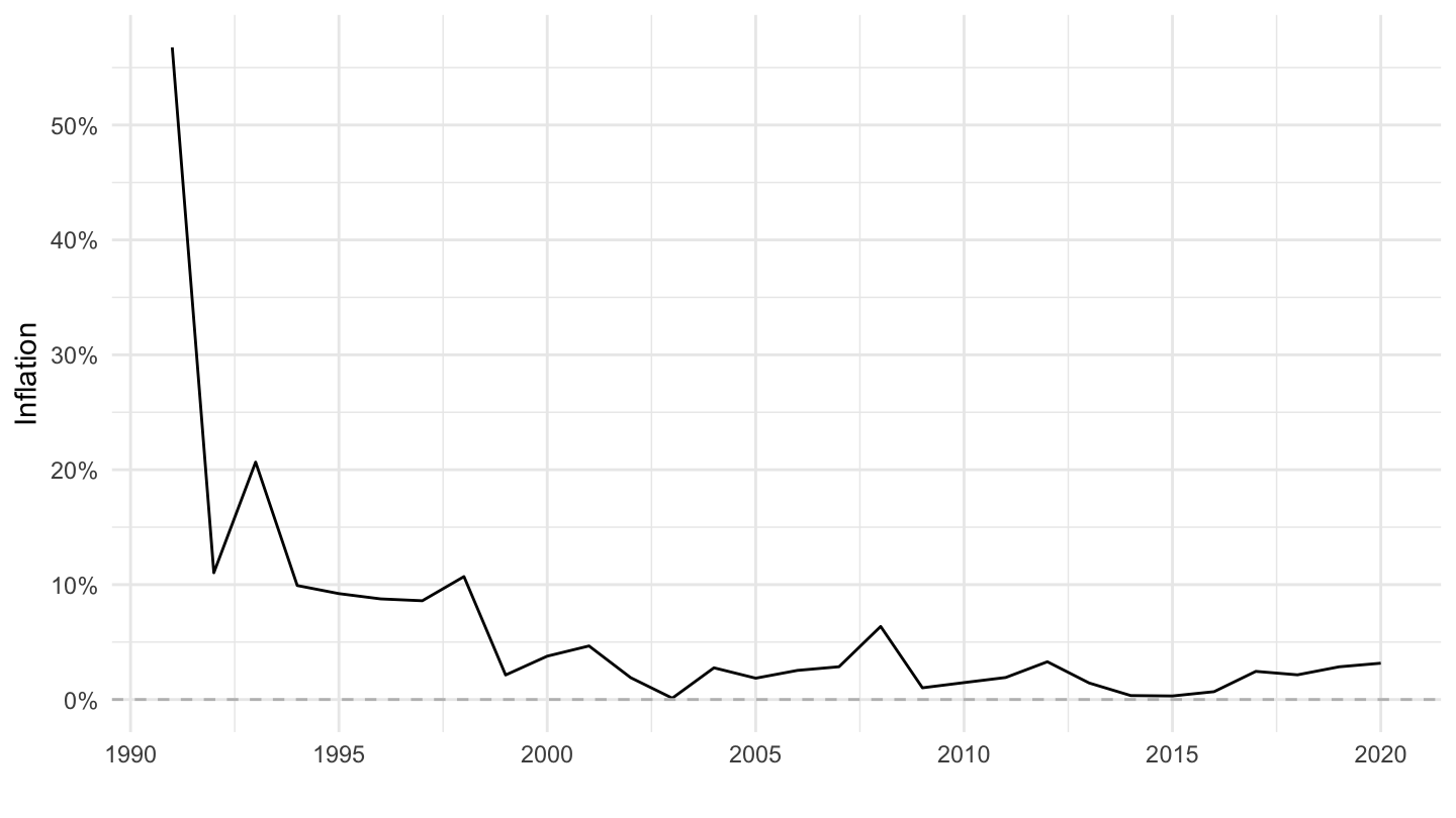
Euro area
Code
CPI %>%
  filter(iso2c %in% c("XM"),
         UNIT_MEASURE == 771,
         FREQ == "A") %>%
  ggplot(.) + geom_line() + theme_minimal() +
  aes(x = date, y = value/100) + xlab("") + ylab("Inflation") +
  scale_x_date(breaks = seq(1900, 2100, 5) %>% paste0("-01-01") %>% as.Date,
               labels = date_format("%Y")) +
  scale_y_continuous(breaks = 0.01*seq(-100, 10000, 1),
                     labels = percent_format(a = 1)) +
  geom_hline(yintercept = 0, linetype = "dashed", color = "grey")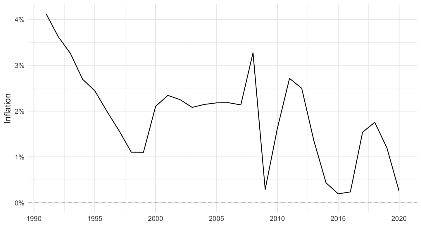
Saudi Arabia
Code
CPI %>%
  filter(iso3c == "SAU",
         UNIT_MEASURE == 771,
         FREQ == "A") %>%
  ggplot(.) + geom_line() + theme_minimal() +
  aes(x = date, y = value/100) + xlab("") + ylab("Inflation") +
  scale_x_date(breaks = seq(1900, 2100, 5) %>% paste0("-01-01") %>% as.Date,
               labels = date_format("%Y")) +
  scale_y_continuous(breaks = 0.01*seq(-100, 10000, 1),
                     labels = percent_format(a = 1)) +
  geom_hline(yintercept = 0, linetype = "dashed", color = "grey")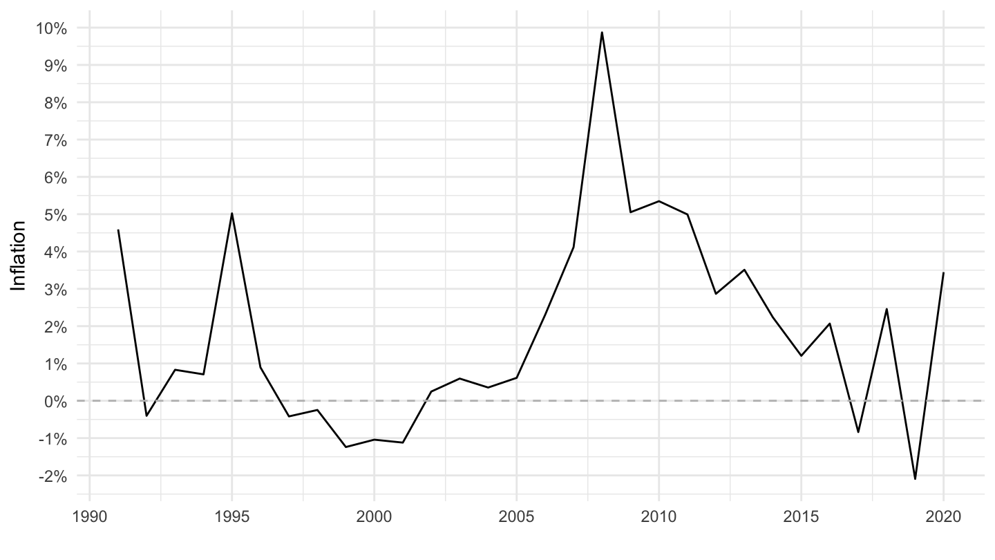
Slovak Republic
Code
CPI %>%
  filter(iso3c == c("SVK"),
         UNIT_MEASURE == 771,
         FREQ == "A") %>%
  ggplot(.) + geom_line() + theme_minimal() +
  aes(x = date, y = value/100) + xlab("") + ylab("Inflation") +
  scale_x_date(breaks = seq(1900, 2100, 5) %>% paste0("-01-01") %>% as.Date,
               labels = date_format("%Y")) +
  scale_y_continuous(breaks = 0.01*seq(-100, 10000, 10),
                     labels = percent_format(a = 1)) +
  geom_hline(yintercept = 0, linetype = "dashed", color = "grey")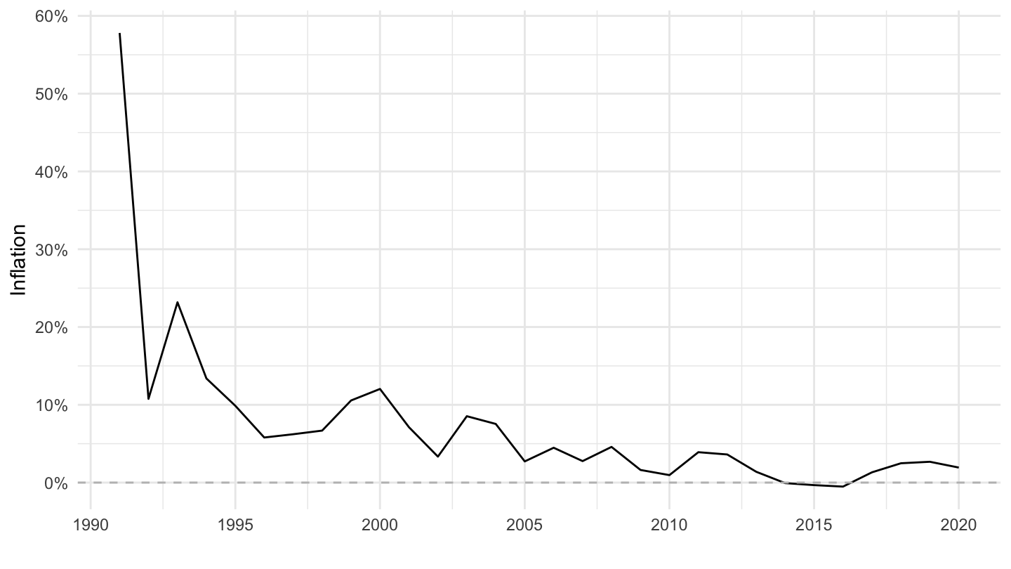
Bulgaria
Code
CPI %>%
  filter(iso3c == "BGR",
         UNIT_MEASURE == 771,
         FREQ == "A") %>%
  ggplot(.) + geom_line() + theme_minimal() +
  aes(x = date, y = value/100) + xlab("") + ylab("Inflation") +
  scale_x_date(breaks = seq(1900, 2100, 5) %>% paste0("-01-01") %>% as.Date,
               labels = date_format("%Y")) +
  scale_y_continuous(breaks = 0.01*seq(-100, 10000, 100),
                     labels = percent_format(a = 1)) +
  geom_hline(yintercept = 0, linetype = "dashed", color = "grey")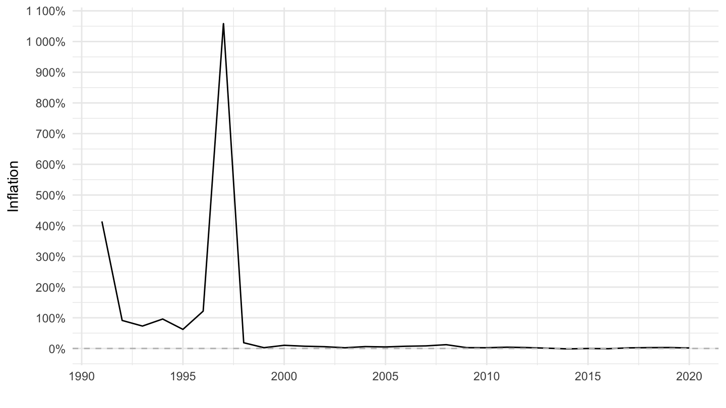
Romania
Code
CPI %>%
  filter(iso3c == "ROU",
         UNIT_MEASURE == 771,
         FREQ == "A") %>%
  ggplot(.) + geom_line() + theme_minimal() +
  aes(x = date, y = value/100) + xlab("") + ylab("Inflation") +
  scale_x_date(breaks = seq(1900, 2100, 5) %>% paste0("-01-01") %>% as.Date,
               labels = date_format("%Y")) +
  scale_y_continuous(breaks = 0.01*seq(-100, 10000, 100),
                     labels = percent_format(a = 1)) +
  geom_hline(yintercept = 0, linetype = "dashed", color = "grey")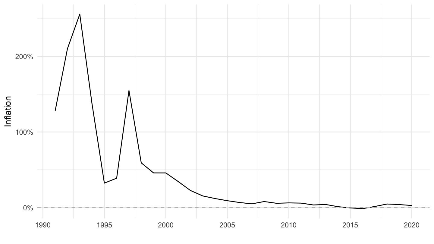
Lithuania
Code
CPI %>%
  filter(iso3c == "LTU",
         UNIT_MEASURE == 771,
         FREQ == "A") %>%
  ggplot(.) + geom_line() + theme_minimal() +
  aes(x = date, y = value/100) + xlab("") + ylab("Inflation") +
  scale_x_date(breaks = seq(1900, 2100, 5) %>% paste0("-01-01") %>% as.Date,
               labels = date_format("%Y")) +
  scale_y_continuous(breaks = 0.01*seq(-100, 10000, 100),
                     labels = percent_format(a = 1)) +
  geom_hline(yintercept = 0, linetype = "dashed", color = "grey")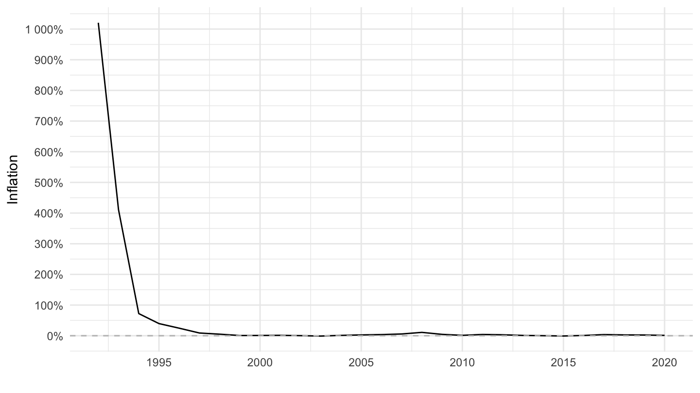
Latvia
Code
CPI %>%
  filter(iso3c == "LVA",
         UNIT_MEASURE == 771,
         FREQ == "A") %>%
  ggplot(.) + geom_line() + theme_minimal() +
  aes(x = date, y = value/100) + xlab("") + ylab("Inflation") +
  scale_x_date(breaks = seq(1900, 2100, 5) %>% paste0("-01-01") %>% as.Date,
               labels = date_format("%Y")) +
  scale_y_continuous(breaks = 0.01*seq(-100, 10000, 100),
                     labels = percent_format(a = 1)) +
  geom_hline(yintercept = 0, linetype = "dashed", color = "grey")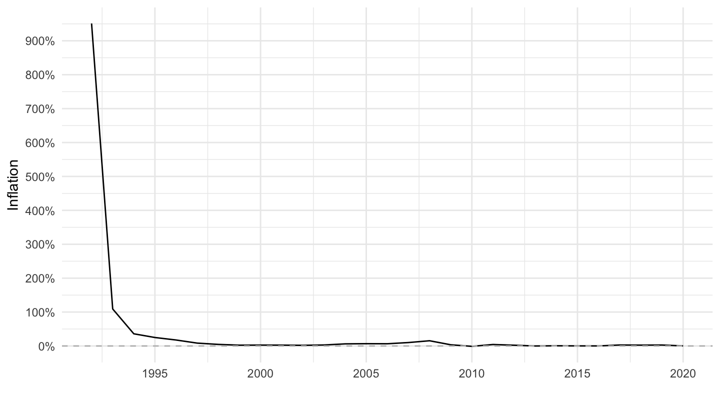
North Macedonia
Code
CPI %>%
  filter(iso3c == "MKD",
         UNIT_MEASURE == 771,
         FREQ == "A") %>%
  ggplot(.) + geom_line() + theme_minimal() +
  aes(x = date, y = value/100) + xlab("") + ylab("Inflation") +
  scale_x_date(breaks = seq(1900, 2100, 5) %>% paste0("-01-01") %>% as.Date,
               labels = date_format("%Y")) +
  scale_y_continuous(breaks = 0.01*seq(-100, 10000, 100),
                     labels = percent_format(a = 1)) +
  geom_hline(yintercept = 0, linetype = "dashed", color = "grey")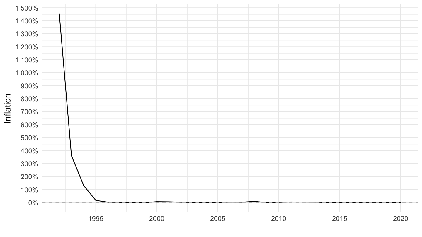
Hungary
Code
CPI %>%
  filter(iso3c == "HUN",
         UNIT_MEASURE == 771,
         FREQ == "A") %>%
  ggplot(.) + geom_line() + theme_minimal() +
  aes(x = date, y = value/100) + xlab("") + ylab("Inflation") +
  scale_x_date(breaks = seq(1900, 2100, 5) %>% paste0("-01-01") %>% as.Date,
               labels = date_format("%Y")) +
  scale_y_continuous(breaks = 0.01*seq(-100, 10000, 2),
                     labels = percent_format(a = 1)) +
  geom_hline(yintercept = 0, linetype = "dashed", color = "grey")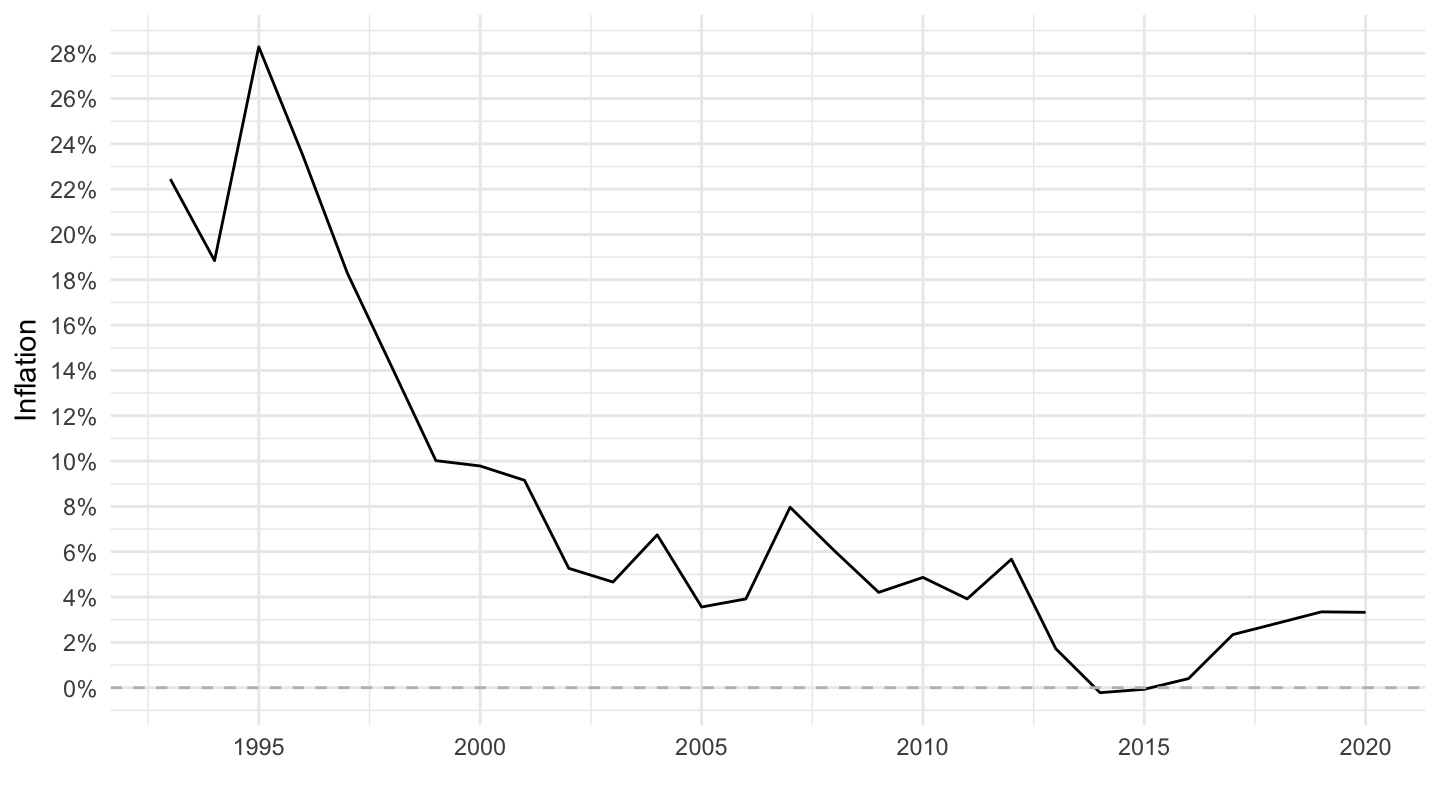
Croatia
Code
CPI %>%
  filter(iso3c == "HRV",
         UNIT_MEASURE == 771,
         FREQ == "A") %>%
  ggplot(.) + geom_line() + theme_minimal() +
  aes(x = date, y = value/100) + xlab("") + ylab("Inflation") +
  scale_x_date(breaks = seq(1900, 2100, 5) %>% paste0("-01-01") %>% as.Date,
               labels = date_format("%Y")) +
  scale_y_continuous(breaks = 0.01*seq(-100, 10000, 100),
                     labels = percent_format(a = 1)) +
  geom_hline(yintercept = 0, linetype = "dashed", color = "grey")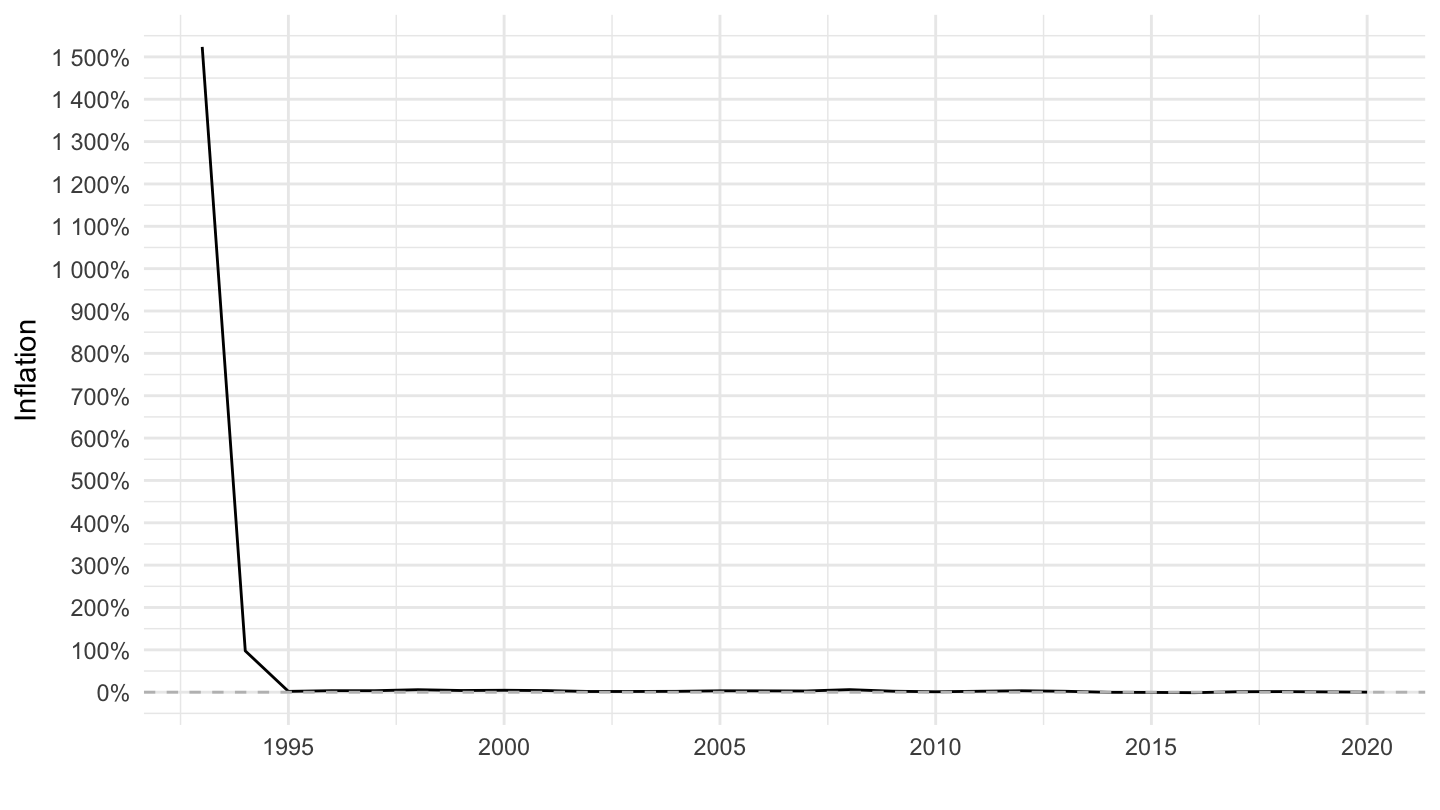
Slovenia
Code
CPI %>%
  filter(iso3c == "SVN",
         UNIT_MEASURE == 771,
         FREQ == "A") %>%
  ggplot(.) + geom_line() + theme_minimal() +
  aes(x = date, y = value/100) + xlab("") + ylab("Inflation") +
  scale_x_date(breaks = seq(1900, 2100, 5) %>% paste0("-01-01") %>% as.Date,
               labels = date_format("%Y")) +
  scale_y_continuous(breaks = 0.01*seq(-100, 10000, 5),
                     labels = percent_format(a = 1)) +
  geom_hline(yintercept = 0, linetype = "dashed", color = "grey")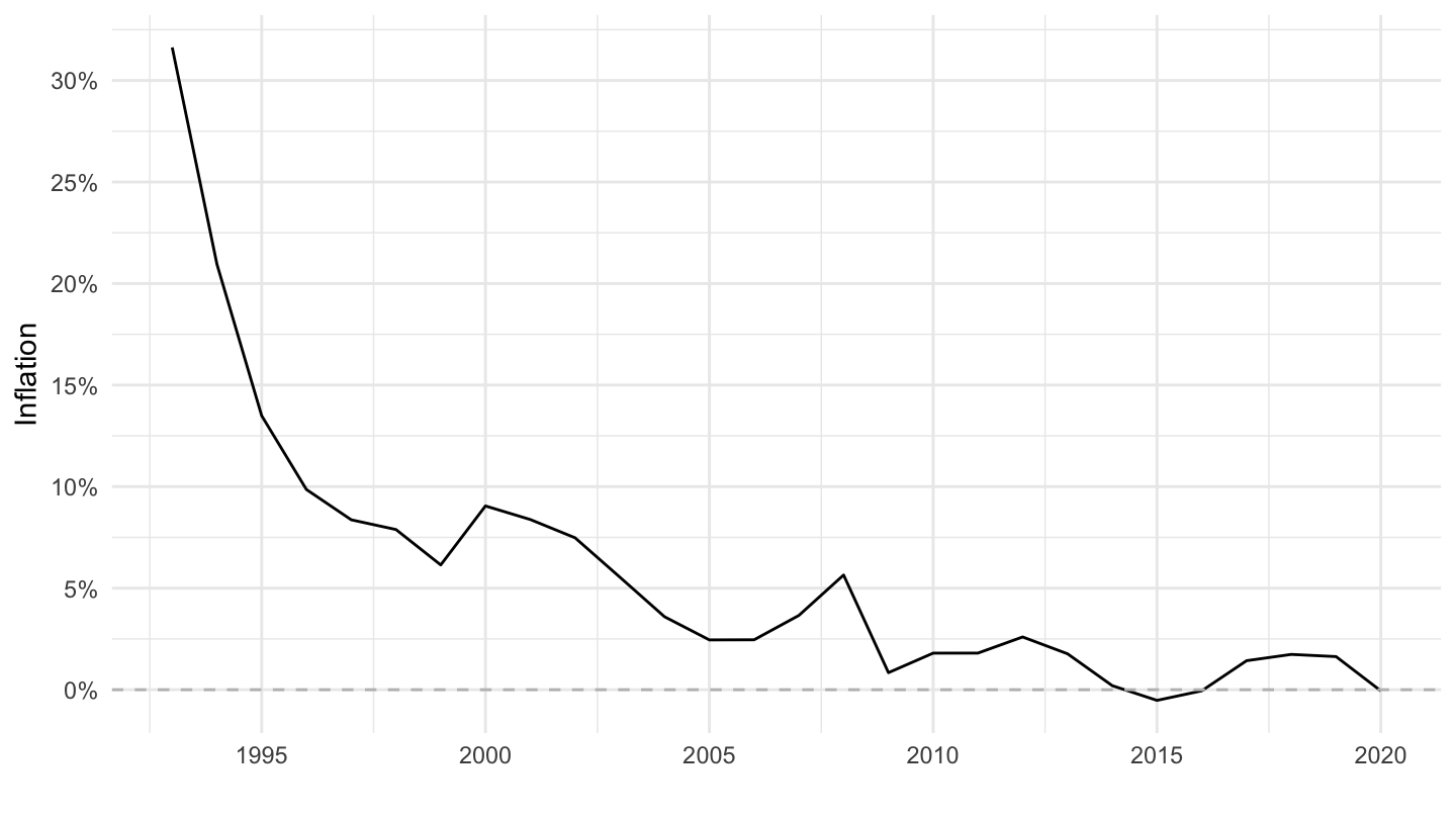
Estonia
Code
CPI %>%
  filter(iso3c == "EST",
         UNIT_MEASURE == 771,
         FREQ == "A") %>%
  ggplot(.) + geom_line() + theme_minimal() +
  aes(x = date, y = value/100) + xlab("") + ylab("Inflation") +
  scale_x_date(breaks = seq(1900, 2100, 5) %>% paste0("-01-01") %>% as.Date,
               labels = date_format("%Y")) +
  scale_y_continuous(breaks = 0.01*seq(-100, 10000, 5),
                     labels = percent_format(a = 1)) +
  geom_hline(yintercept = 0, linetype = "dashed", color = "grey")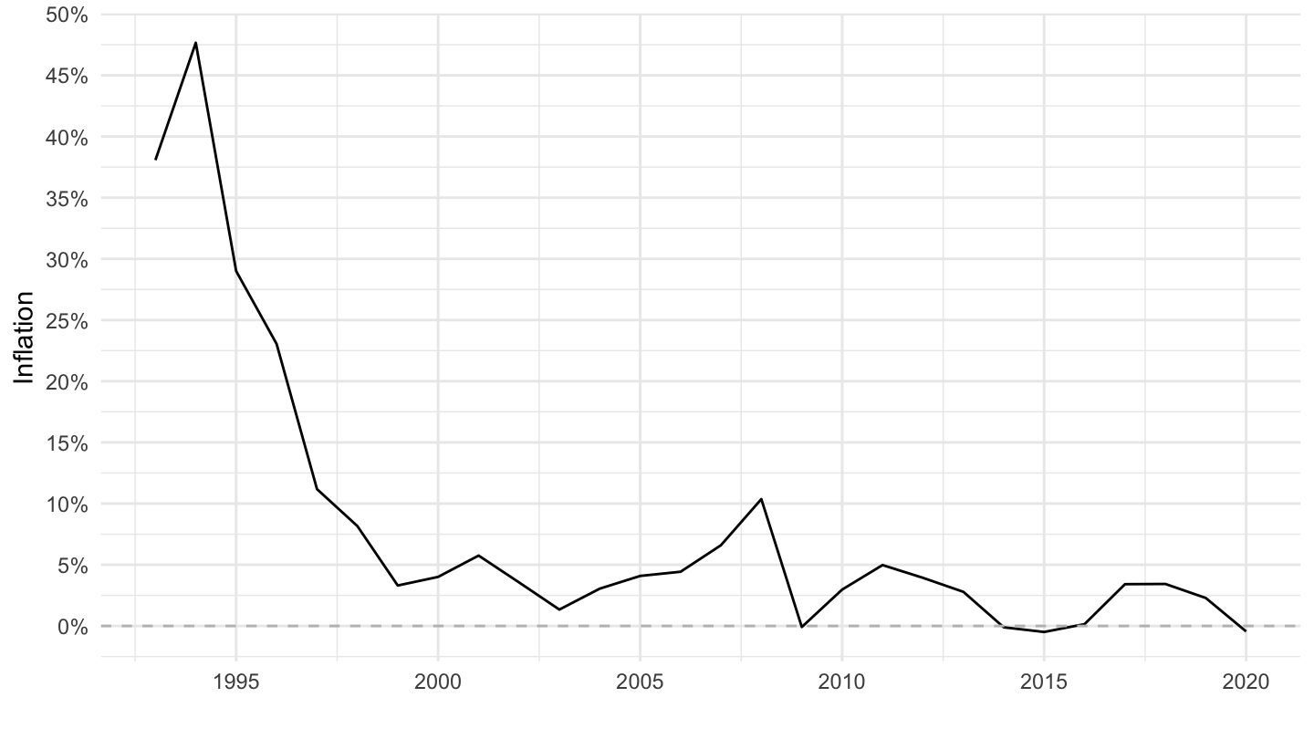
China
Code
CPI %>%
  filter(iso3c == "CHN",
         UNIT_MEASURE == 771,
         FREQ == "A") %>%
  ggplot(.) + geom_line() + theme_minimal() +
  aes(x = date, y = value/100) + xlab("") + ylab("Inflation") +
  scale_x_date(breaks = seq(1900, 2100, 5) %>% paste0("-01-01") %>% as.Date,
               labels = date_format("%Y")) +
  scale_y_continuous(breaks = 0.01*seq(-100, 10000, 5),
                     labels = percent_format(a = 1)) +
  geom_hline(yintercept = 0, linetype = "dashed", color = "grey")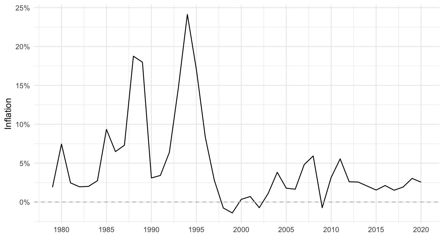
Serbia
Code
CPI %>%
  filter(iso3c == "SRB",
         UNIT_MEASURE == 771,
         FREQ == "A") %>%
  ggplot(.) + geom_line() + theme_minimal() +
  aes(x = date, y = value/100) + xlab("") + ylab("Inflation") +
  scale_x_date(breaks = seq(1900, 2100, 5) %>% paste0("-01-01") %>% as.Date,
               labels = date_format("%Y")) +
  scale_y_continuous(labels = percent_format(a = 1)) +
  geom_hline(yintercept = 0, linetype = "dashed", color = "grey")
Algeria
Code
CPI %>%
  filter(iso3c == "DZA",
         UNIT_MEASURE == 771,
         FREQ == "A") %>%
  ggplot(.) + geom_line() + theme_minimal() +
  aes(x = date, y = value/100) + xlab("") + ylab("Inflation") +
  scale_x_date(breaks = seq(1900, 2100, 5) %>% paste0("-01-01") %>% as.Date,
               labels = date_format("%Y")) +
  scale_y_continuous(breaks = 0.01*seq(-100, 10000, 5),
                     labels = percent_format(a = 1)) +
  geom_hline(yintercept = 0, linetype = "dashed", color = "grey")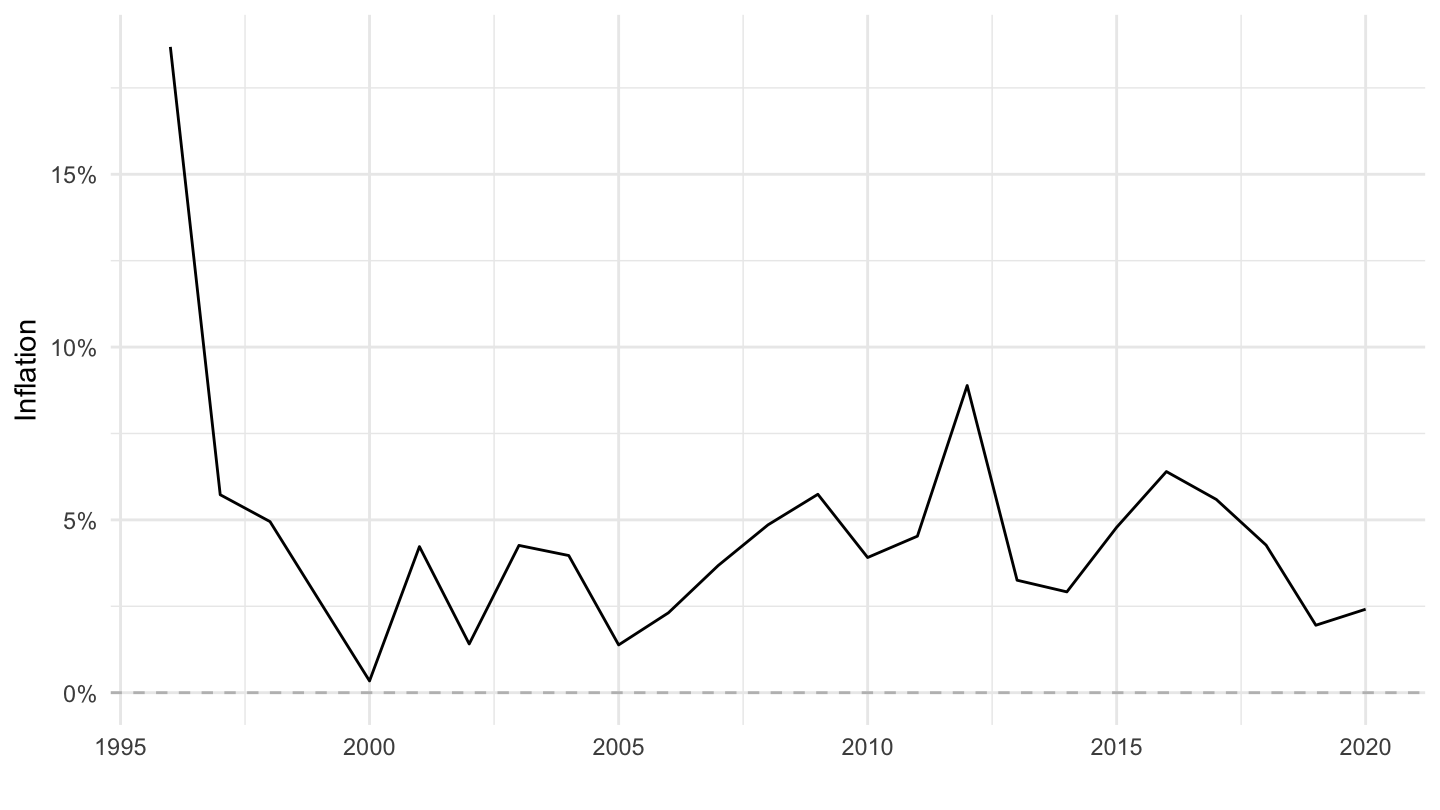
Russia
Code
CPI %>%
  filter(iso3c == "RUS",
         UNIT_MEASURE == 771,
         FREQ == "A") %>%
  ggplot(.) + geom_line() + theme_minimal() +
  aes(x = date, y = value/100) + xlab("") + ylab("Inflation") +
  scale_x_date(breaks = seq(1900, 2100, 5) %>% paste0("-01-01") %>% as.Date,
               labels = date_format("%Y")) +
  scale_y_continuous(breaks = 0.01*seq(-100, 10000, 2),
                     labels = percent_format(a = 1)) +
  geom_hline(yintercept = 0, linetype = "dashed", color = "grey")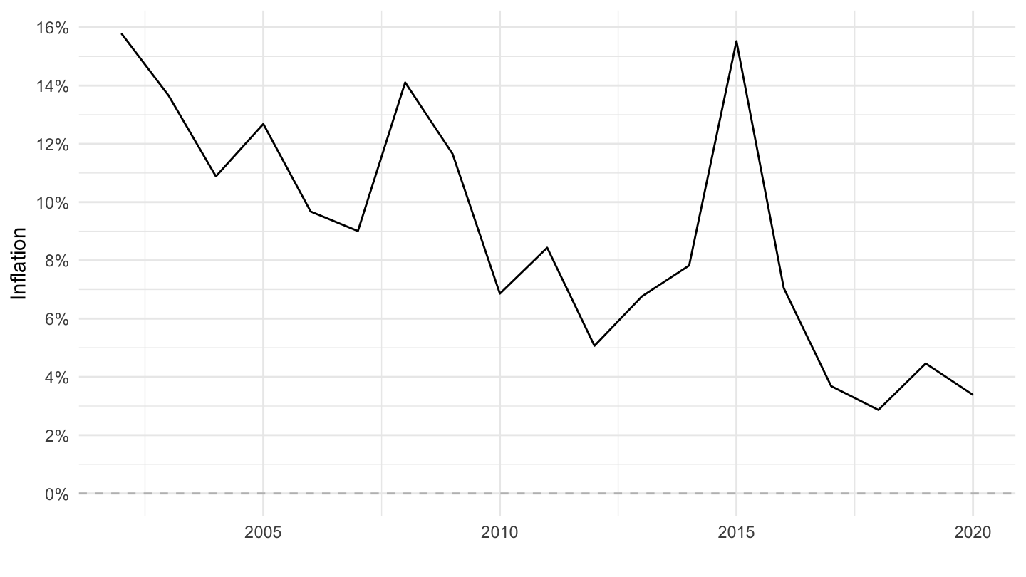
United Arab Emirates
Code
CPI %>%
  filter(iso3c == "ARE",
         UNIT_MEASURE == 771,
         FREQ == "A") %>%
  ggplot(.) + geom_line() + theme_minimal() +
  aes(x = date, y = value/100) + xlab("") + ylab("Inflation") +
  scale_x_date(breaks = seq(1900, 2100, 5) %>% paste0("-01-01") %>% as.Date,
               labels = date_format("%Y")) +
  scale_y_continuous(breaks = 0.01*seq(-100, 10000, 2),
                     labels = percent_format(a = 1)) +
  geom_hline(yintercept = 0, linetype = "dashed", color = "grey")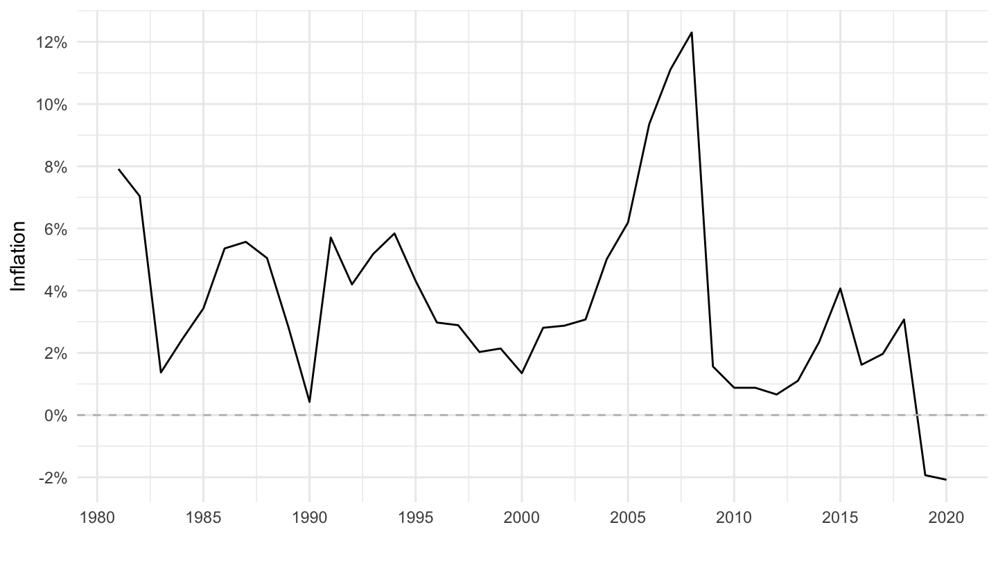
Index (100)
Argentina
All
Code
CPI %>%
  filter(iso3c %in% c("ARG"),
         UNIT_MEASURE == 628,
         FREQ == "A") %>%
  ggplot(.) + geom_line(aes(x = date, y = value)) +
  theme_minimal() + xlab("") + ylab("CPI (Index)") +
  scale_x_date(breaks = seq(1900, 2100, 10) %>% paste0("-01-01") %>% as.Date,
               labels = date_format("%Y")) +
  scale_y_log10(breaks = seq(0, 200, 10),
                     labels = dollar_format(a = 1, p = "")) +
  scale_color_manual(values = viridis(5)[1:4]) +
  theme(legend.position = c(0.2, 0.80),
        legend.title = element_blank()) +
  geom_vline(xintercept = as.Date("2013-03-01"), linetype = "dashed", color = viridis(3)[2])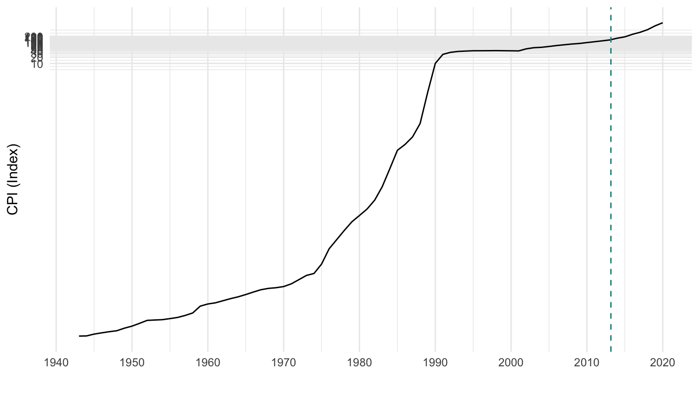
1990-
Code
CPI %>%
  filter(iso3c %in% c("ARG"),
         UNIT_MEASURE == 628,
         FREQ == "A") %>%
  filter(date >= as.Date("1990-01-01")) %>%
  ggplot(.) + geom_line(aes(x = date, y = value)) +
  theme_minimal() + xlab("") + ylab("CPI (Index)") +
  scale_x_date(breaks = seq(1900, 2100, 5) %>% paste0("-01-01") %>% as.Date,
               labels = date_format("%Y")) +
  scale_y_log10(breaks = seq(0, 200, 2),
                     labels = dollar_format(a = 1, p = "")) +
  scale_color_manual(values = viridis(3)[1:2]) +
  theme(legend.position = c(0.2, 0.80),
        legend.title = element_blank()) +
  geom_vline(xintercept = as.Date("2013-03-01"), linetype = "dashed", color = viridis(3)[2])
1990-2005
Code
CPI %>%
  filter(iso3c %in% c("ARG"),
         UNIT_MEASURE == 628,
         FREQ == "A",
         date >= as.Date("1990-01-01"),
         date <= as.Date("2005-01-01")) %>%
  ggplot(.) + geom_line(aes(x = date, y = value)) +
  theme_minimal() + xlab("") + ylab("CPI (Index)") +
  scale_x_date(breaks = seq(1900, 2100, 2) %>% paste0("-01-01") %>% as.Date,
               labels = date_format("%Y")) +
  scale_y_log10(breaks = seq(0, 200, 10),
                     labels = dollar_format(a = 1, p = "")) +
  scale_color_manual(values = viridis(3)[1:2]) +
  theme(legend.position = c(0.2, 0.80),
        legend.title = element_blank()) +
  geom_vline(xintercept = as.Date("2013-03-01"), linetype = "dashed", color = viridis(3)[2])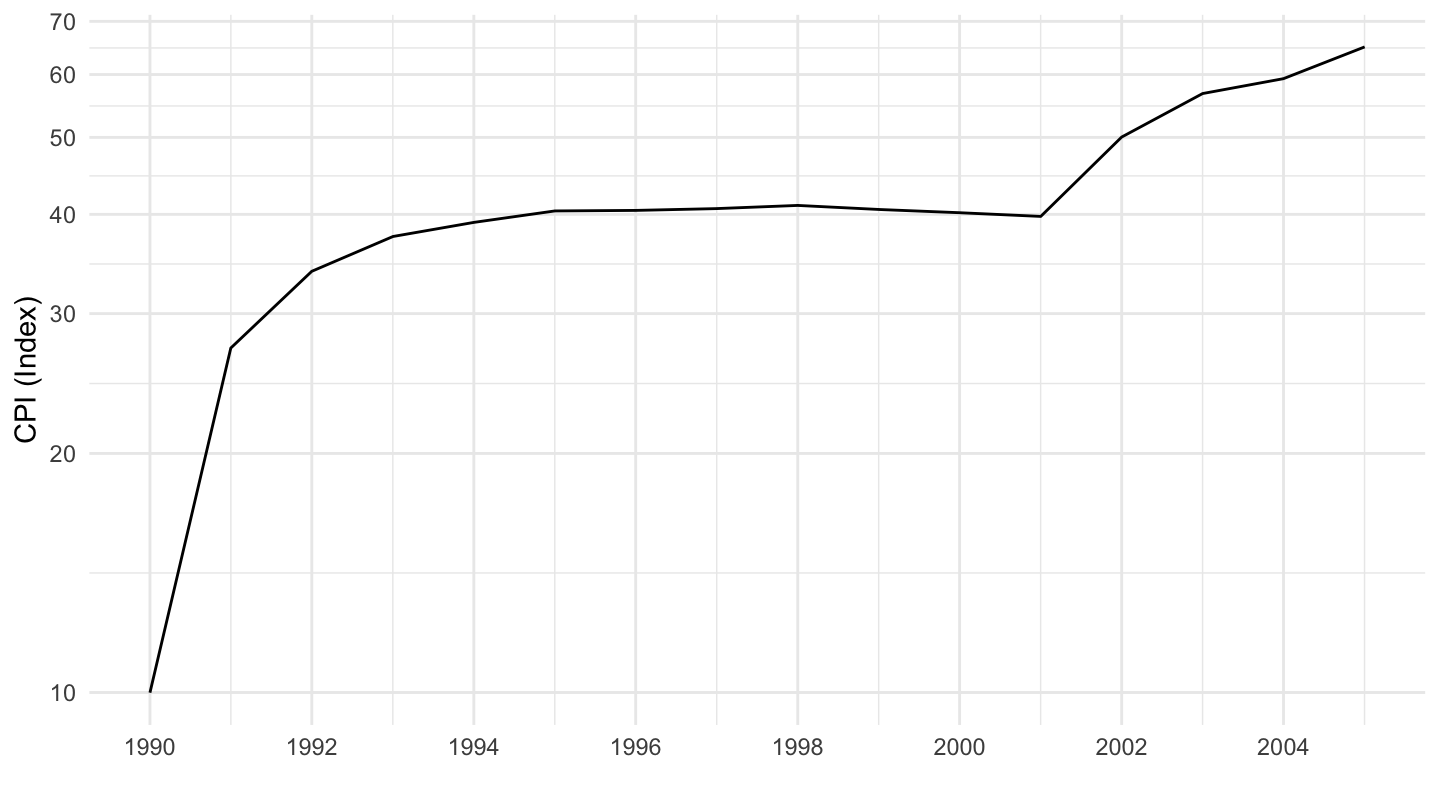
Crisis in Argentina
Code
CPI %>%
  filter(iso3c %in% c("ARG"),
         UNIT_MEASURE == 628,
         FREQ == "A",
         date >= as.Date("1993-01-01"),
         date <= as.Date("2005-01-01")) %>%
  ggplot(.) + geom_line(aes(x = date, y = value)) +
  theme_minimal() + xlab("") + ylab("CPI (Index)") +
  scale_x_date(breaks = seq(1900, 2100, 1) %>% paste0("-01-01") %>% as.Date,
               labels = date_format("%Y")) +
  scale_y_log10(breaks = seq(0, 200, 5),
                     labels = dollar_format(a = 1, p = "")) +
  scale_color_manual(values = viridis(3)[1:2]) +
  theme(legend.position = c(0.2, 0.80),
        legend.title = element_blank()) +
  geom_vline(xintercept = as.Date("2013-03-01"), linetype = "dashed", color = viridis(3)[2])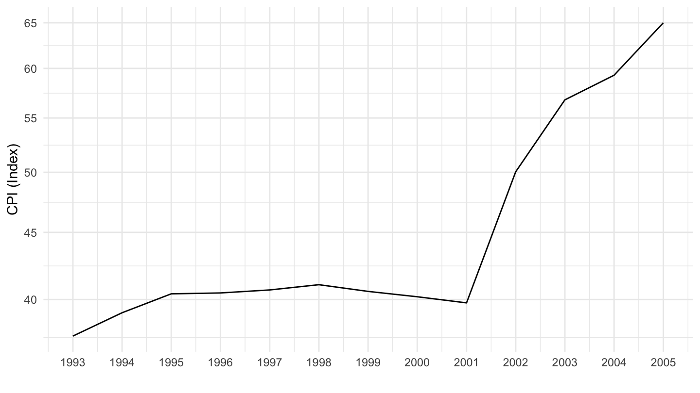
1980-
Code
CPI %>%
  filter(iso3c %in% c("ARG"),
         UNIT_MEASURE == 628,
         FREQ == "A") %>%
  filter(date >= as.Date("1980-01-01")) %>%
  ggplot(.) + geom_line(aes(x = date, y = value)) +
  theme_minimal() + xlab("") + ylab("CPI (Index)") +
  scale_x_date(breaks = seq(1900, 2100, 5) %>% paste0("-01-01") %>% as.Date,
               labels = date_format("%Y")) +
  scale_y_log10(breaks = seq(0, 200, 2),
                     labels = dollar_format(a = 1, p = "")) +
  scale_color_manual(values = viridis(3)[1:2]) +
  theme(legend.position = c(0.2, 0.80),
        legend.title = element_blank()) +
  geom_vline(xintercept = as.Date("2013-03-01"), linetype = "dashed", color = viridis(3)[2])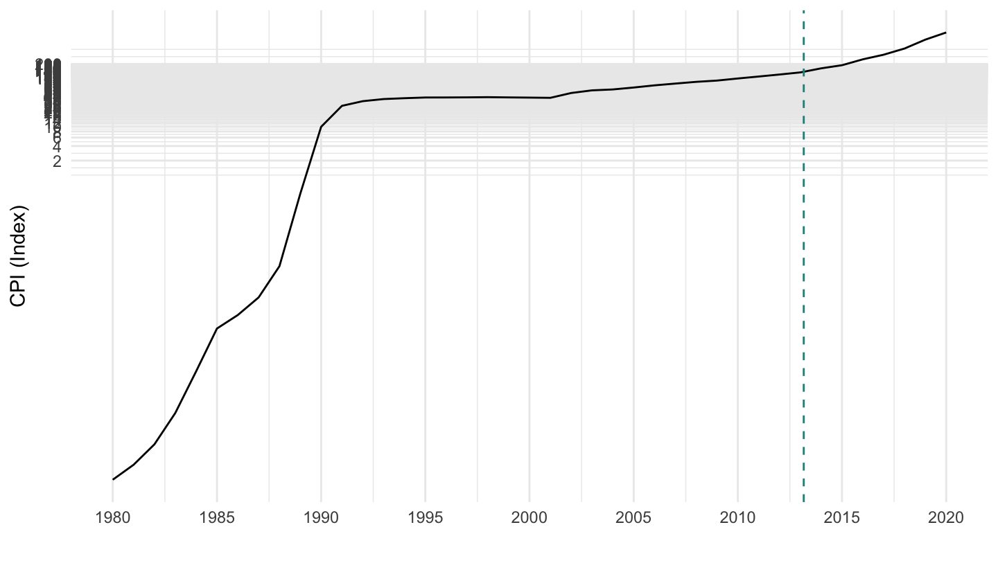
Japan
All
Code
CPI %>%
  filter(iso3c %in% c("JPN"),
         UNIT_MEASURE == 628,
         FREQ == "A") %>%
  ggplot(.) + geom_line(aes(x = date, y = value)) +
  theme_minimal() + xlab("") + ylab("CPI (Index)") +
  scale_x_date(breaks = seq(1900, 2100, 10) %>% paste0("-01-01") %>% as.Date,
               labels = date_format("%Y")) +
  scale_y_log10(breaks = seq(0, 200, 10),
                     labels = dollar_format(a = 1, p = "")) +
  scale_color_manual(values = viridis(5)[1:4]) +
  theme(legend.position = c(0.2, 0.80),
        legend.title = element_blank()) +
  geom_vline(xintercept = as.Date("2013-03-01"), linetype = "dashed", color = viridis(3)[2])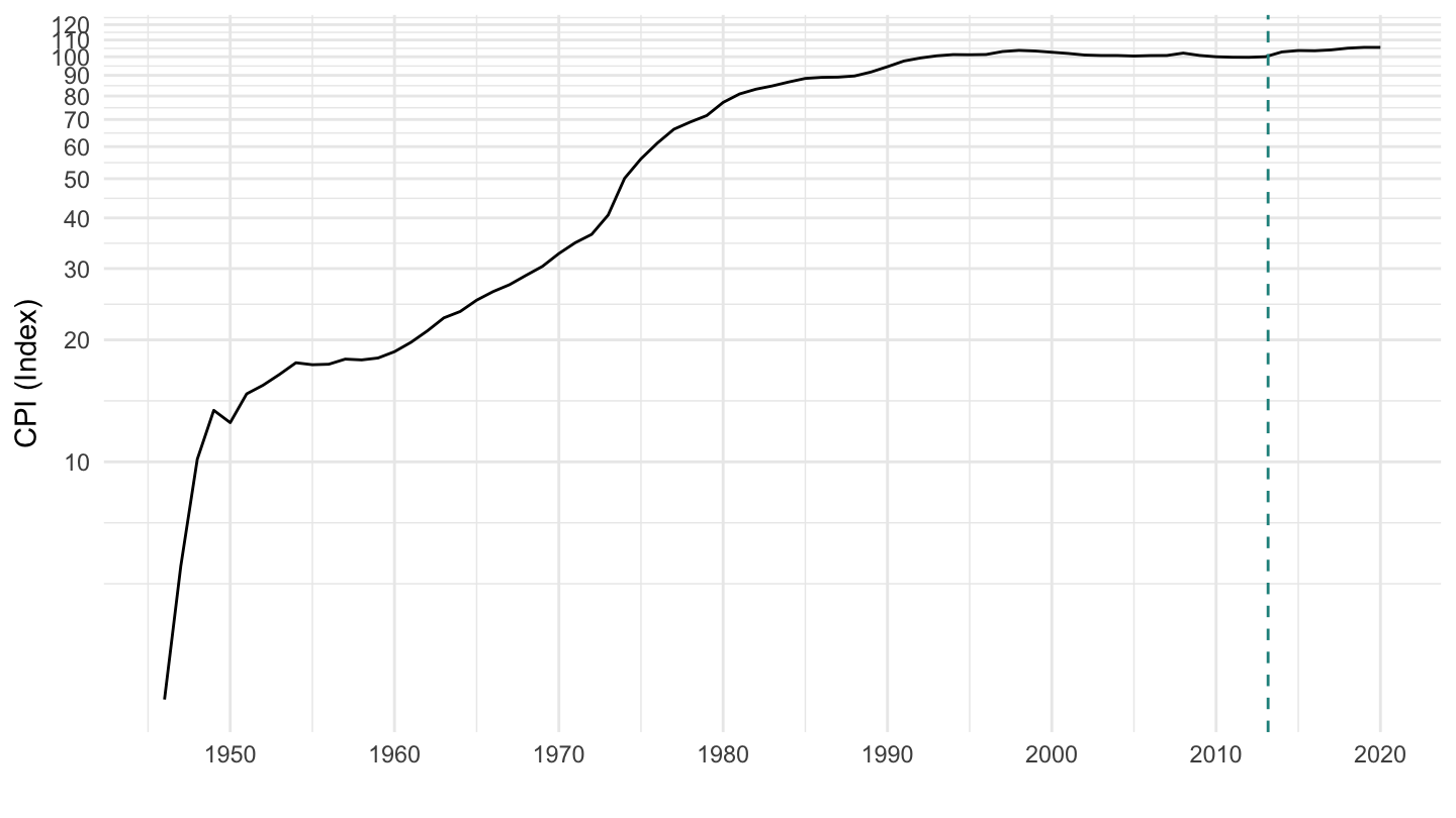
1990-
Code
CPI %>%
  filter(iso3c %in% c("JPN"),
         UNIT_MEASURE == 628,
         FREQ == "A") %>%
  filter(date >= as.Date("1990-01-01")) %>%
  ggplot(.) + geom_line(aes(x = date, y = value)) +
  theme_minimal() + xlab("") + ylab("CPI (Index)") +
  scale_x_date(breaks = seq(1900, 2100, 5) %>% paste0("-01-01") %>% as.Date,
               labels = date_format("%Y")) +
  scale_y_log10(breaks = seq(0, 200, 2),
                     labels = dollar_format(a = 1, p = "")) +
  scale_color_manual(values = viridis(3)[1:2]) +
  theme(legend.position = c(0.2, 0.80),
        legend.title = element_blank()) +
  geom_vline(xintercept = as.Date("2013-03-01"), linetype = "dashed", color = viridis(3)[2])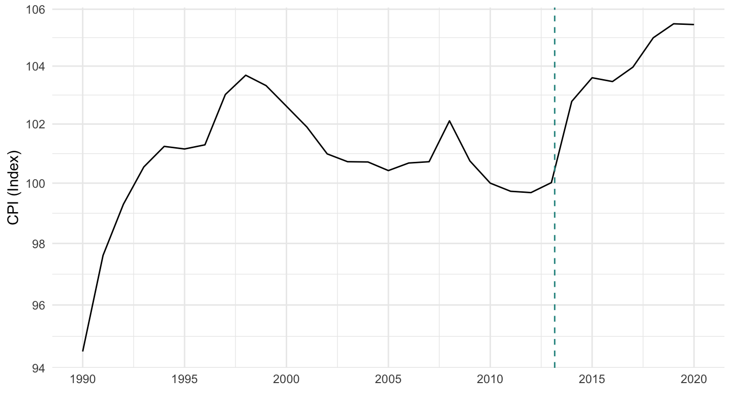
1980-
Code
CPI %>%
  filter(iso3c %in% c("JPN"),
         UNIT_MEASURE == 628,
         FREQ == "A") %>%
  filter(date >= as.Date("1980-01-01")) %>%
  ggplot(.) + geom_line(aes(x = date, y = value)) +
  theme_minimal() + xlab("") + ylab("CPI (Index)") +
  scale_x_date(breaks = seq(1900, 2100, 5) %>% paste0("-01-01") %>% as.Date,
               labels = date_format("%Y")) +
  scale_y_log10(breaks = seq(0, 200, 2),
                     labels = dollar_format(a = 1, p = "")) +
  scale_color_manual(values = viridis(3)[1:2]) +
  theme(legend.position = c(0.2, 0.80),
        legend.title = element_blank()) +
  geom_vline(xintercept = as.Date("2013-03-01"), linetype = "dashed", color = viridis(3)[2])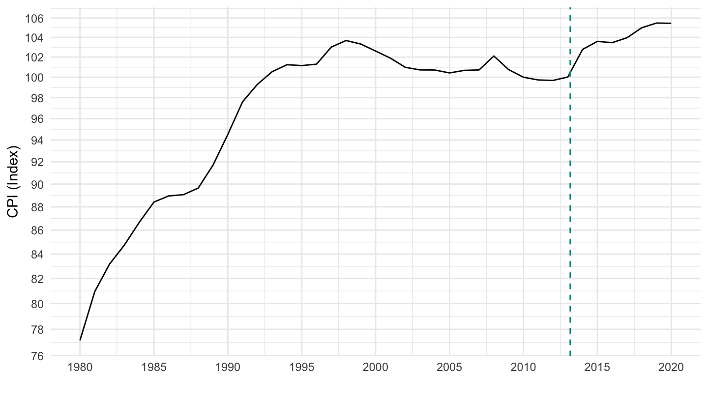
Germany, France, Italy, Spain
Code
CPI %>%
  filter(iso3c %in% c("DEU", "FRA", "ITA", "ESP"),
         UNIT_MEASURE == 628,
         FREQ == "A") %>%
  ggplot(.) + geom_line(aes(x = date, y = value, color = `Reference area`)) +
  theme_minimal() + xlab("") + ylab("CPI (Index)") +
  scale_x_date(breaks = seq(1900, 2100, 10) %>% paste0("-01-01") %>% as.Date,
               labels = date_format("%Y")) +
  scale_y_log10(breaks = seq(0, 200, 10),
                     labels = dollar_format(a = 1, p = "")) +
  scale_color_manual(values = viridis(5)[1:4]) +
  theme(legend.position = c(0.2, 0.80),
        legend.title = element_blank())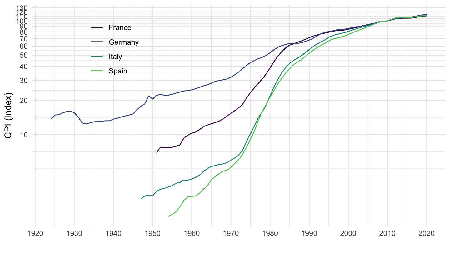
Germany, France, United States
Code
CPI %>%
  filter(iso3c %in% c("DEU", "FRA", "USA"),
         UNIT_MEASURE == 628,
         FREQ == "A",
         date >= as.Date("1990-01-01")) %>%
  group_by(iso3c) %>%
  mutate(value = 100*value/value[date == as.Date("1990-01-01")]) %>%
  ggplot(.) + geom_line(aes(x = date, y = value, color = `Reference area`)) +
  theme_minimal() + xlab("") + ylab("CPI (Index)") +
  scale_x_date(breaks = seq(1900, 2100, 5) %>% paste0("-01-01") %>% as.Date,
               labels = date_format("%Y")) +
  scale_y_log10(breaks = c(seq(0, 200, 10), seq(200, 1000, 20)),
                labels = dollar_format(a = 1, p = "")) +
  scale_color_manual(values = viridis(4)[1:3]) +
  theme(legend.position = c(0.2, 0.80),
        legend.title = element_blank())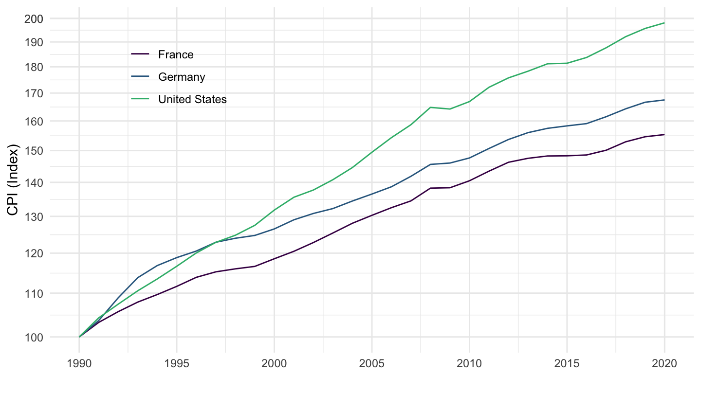
Canada, UK, Norway, USA
Code
CPI %>%
  filter(iso3c %in% c("GBR", "USA", "CAN", "NOR"),
         UNIT_MEASURE == 628,
         FREQ == "A") %>%
  ggplot(.) + geom_line(aes(x = date, y = value, color = `Reference area`)) +
  theme_minimal() + xlab("") + ylab("CPI (Index)") +
  scale_x_date(breaks = seq(1600, 2100, 50) %>% paste0("-01-01") %>% as.Date,
               labels = date_format("%Y")) +
  scale_y_log10(breaks = seq(0, 200, 10),
                     labels = dollar_format(accuracy = 1, prefix = "")) +
  scale_color_manual(values = viridis(5)[1:4]) +
  theme(legend.position = c(0.2, 0.80),
        legend.title = element_blank())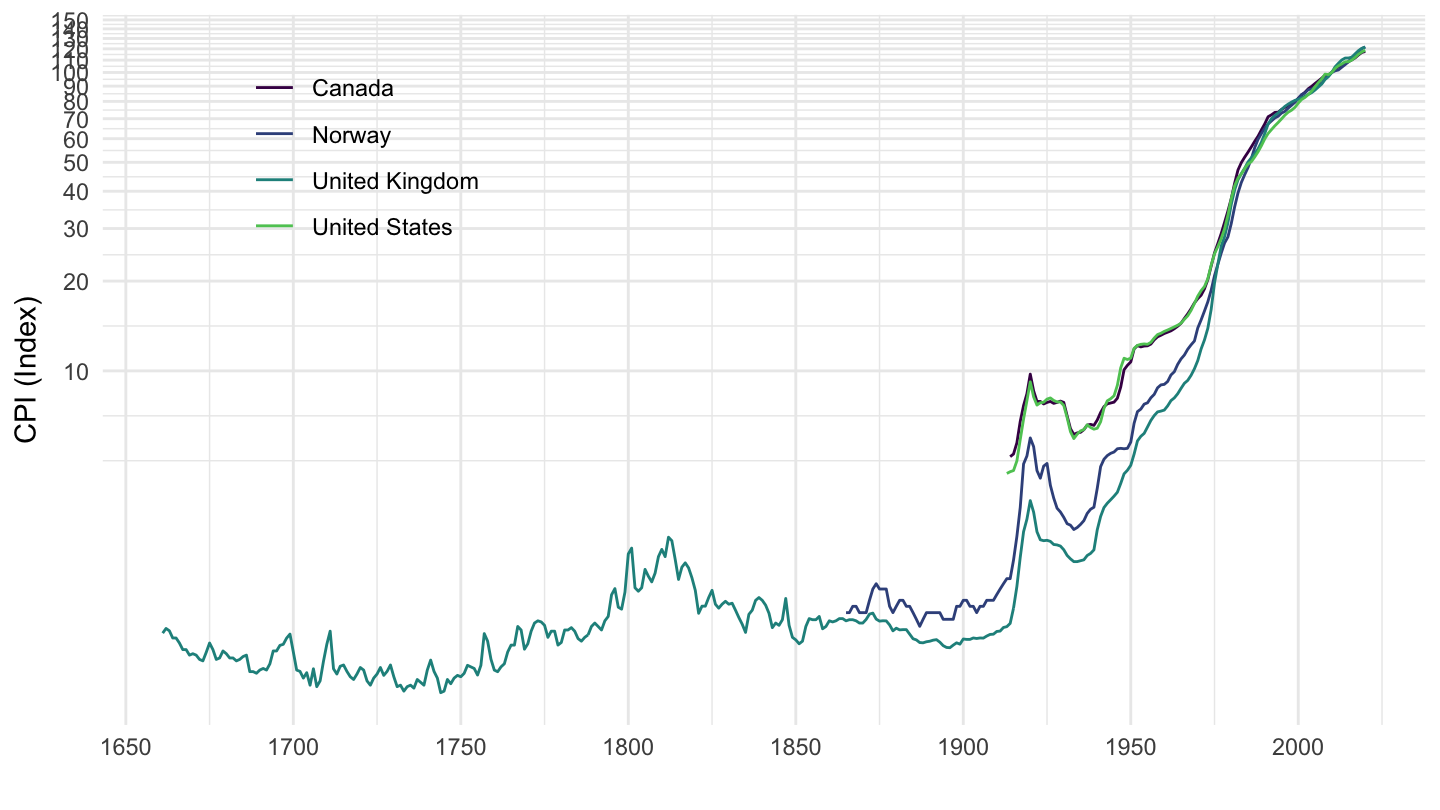
Canada, UK, Norway, USA (1920-)
Code
CPI %>%
  filter(iso3c %in% c("GBR", "USA", "CAN", "NOR"),
         UNIT_MEASURE == 628,
         FREQ == "A") %>%
  filter(date >= as.Date("1910-01-01")) %>%
  ggplot(.) + geom_line(aes(x = date, y = value, color = `Reference area`)) +
  theme_minimal() + xlab("") + ylab("CPI (Index)") +
  scale_x_date(breaks = seq(1600, 2100, 10) %>% paste0("-01-01") %>% as.Date,
               labels = date_format("%Y")) +
  scale_y_log10(breaks = seq(0, 200, 10),
                labels = dollar_format(accuracy = 1, prefix = "")) +
  scale_color_manual(values = viridis(5)[1:4]) +
  theme(legend.position = c(0.2, 0.80),
        legend.title = element_blank())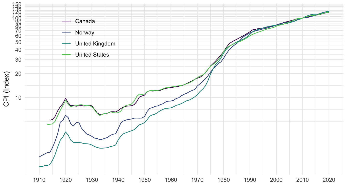
Canada, UK, Norway, USA (1910-1950)
Code
CPI %>%
  filter(iso3c %in% c("GBR", "USA", "CAN", "NOR"),
         UNIT_MEASURE == 628,
         FREQ == "A",
         date >= as.Date("1910-01-01"),
         date <= as.Date("1950-01-01")) %>%
  ggplot(.) + geom_line(aes(x = date, y = value, color = `Reference area`)) +
  theme_minimal() + xlab("") + ylab("CPI (Index)") +
  scale_x_date(breaks = seq(1600, 2100, 10) %>% paste0("-01-01") %>% as.Date,
               labels = date_format("%Y")) +
  scale_y_log10(breaks = seq(0, 20, 1),
                labels = dollar_format(accuracy = 1, prefix = "")) +
  scale_color_manual(values = viridis(5)[1:4]) +
  theme(legend.position = c(0.1, 0.85),
        legend.title = element_blank())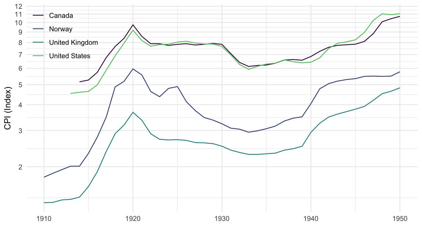
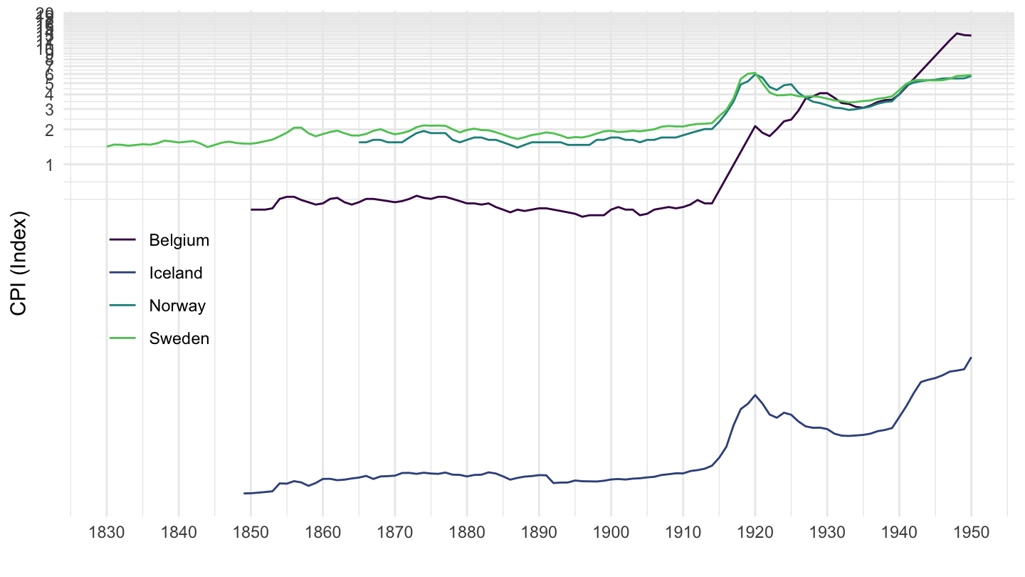
Sweden, Iceland, Belgium, Norway (1910-1950)
Code
CPI %>%
  filter(iso3c %in% c("SWE", "ISL", "BEL", "NOR"),
         UNIT_MEASURE == 628,
         FREQ == "A",
         date >= as.Date("1800-01-01"),
         date <= as.Date("1950-01-01")) %>%
  ggplot(.) + geom_line(aes(x = date, y = value, color = `Reference area`)) +
  theme_minimal() + xlab("") + ylab("CPI (Index)") +
  scale_x_date(breaks = seq(1600, 2100, 10) %>% paste0("-01-01") %>% as.Date,
               labels = date_format("%Y")) +
  scale_y_log10(breaks = seq(0, 20, 1),
                labels = dollar_format(accuracy = 1, prefix = "")) +
  scale_color_manual(values = viridis(5)[1:4]) +
  theme(legend.position = c(0.1, 0.45),
        legend.title = element_blank())