Inflation
Data - Fred
Info
LAST_COMPILE
| LAST_COMPILE |
|---|
| 2026-07-23 |
Last
| date | Nobs |
|---|---|
| 2026-07-23 | 3 |
variable
| variable | Variable | Nobs |
|---|---|---|
| T10YIE | 10-Year Breakeven Inflation Rate | 6146 |
| T5YIE | 5-Year Breakeven Inflation Rate | 6146 |
| T5YIFR | 5-Year, 5-Year Forward Inflation Expectation Rate | 6146 |
| GASREGW | US Regular All Formulations Gas Price | 1875 |
| CUUR0000SA0L2 | Consumer Price Index for All Urban Consumers: All Items Less Shelter in U.S. City Average | 1096 |
| CPIAUCSL | Consumer Price Index for All Urban Consumers: All Items in U.S. City Average | 954 |
| UNRATE | Unemployment Rate | 942 |
| CUUR0000SAH1 | Consumer Price Index for All Urban Consumers: Shelter in U.S. City Average | 883 |
| CPILFESL | Consumer Price Index for All Urban Consumers: All Items Less Food and Energy in U.S. City Average | 834 |
| PCEPI | Personal Consumption Expenditures: Chain-type Price Index | 809 |
| PCEPILFE | Personal Consumption Expenditures Excluding Food and Energy (Chain-Type Price Index) | 809 |
| MICH | University of Michigan: Inflation Expectation | 581 |
| CP0000USM086NEST | Harmonized Index of Consumer Prices: Total for United States | 325 |
| CP00MI15EA20M086NEST | Harmonized Index of Consumer Prices: Total for Euro Area (20 Countries) | 319 |
| TOTNRGFOODEA20MI15XM | Harmonized Index of Consumer Prices: Overall Index Excluding Energy, Food, Alcohol, and Tobacco for Euro Area (20 Countries) | 319 |
| A255RD3Q086SBEA | Imports of goods (implicit price deflator) | 317 |
| GDPDEF | Gross Domestic Product: Implicit Price Deflator | 317 |
| T7YIEM | 7-year Breakeven Inflation Rate | 282 |
| DPCCRV1Q225SBEA | Personal Consumption Expenditures (PCE) Excluding Food and Energy (Chain-Type Price Index) | 268 |
| T20YIEM | 20-year Breakeven Inflation Rate | 264 |
| T30YIEM | 30-year Breakeven Inflation Rate | 197 |
| FPCPITOTLZGUSA | Inflation, consumer prices for the United States | 65 |
CPI, HICP
All
Code
inflation %>%
  filter(variable %in% c("CPIAUCSL", "CP00MI15EA20M086NEST")) %>%
  select(date, variable, value) %>%
  group_by(variable) %>%
  arrange(date) %>%
  mutate(value = value/lag(value, 12) - 1) %>%
  mutate(country = ifelse(variable == "CP00MI15EA20M086NEST", "Euro area (HICP)", "US (CPI)")) %>%
  na.omit %>%
  #filter(value >= 0.14) %>%
  ggplot(.) + geom_line(aes(x = date, y = value, color = country)) + theme_minimal() +
  scale_x_date(breaks = "5 years",
               labels = date_format("%Y")) +
  scale_y_continuous(breaks = 0.01*seq(-60, 60, 1),
                     labels = scales::percent_format(accuracy = 1)) +
  scale_color_manual(values = c("#003399", "#B22234")) +
  xlab("") + ylab("Inflation (%)") +
  theme(legend.position = c(0.2, 0.9),
        legend.title = element_blank(),
        axis.text.x = element_text(angle = 45, vjust = 1, hjust = 1)) +
  geom_hline(yintercept = 0.02, linetype = "dashed")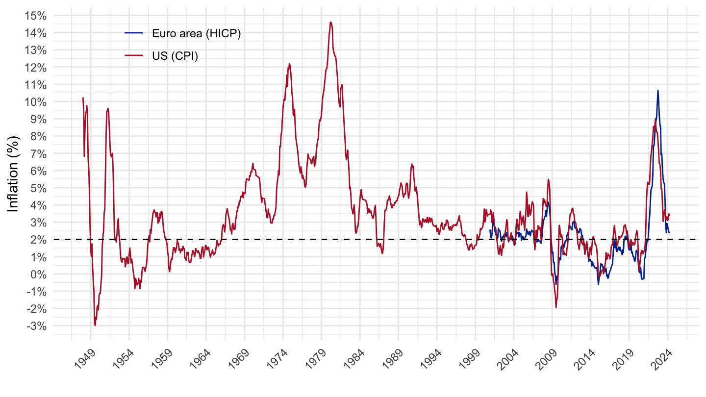
Since 2020
All
Code
inflation %>%
  filter(variable %in% c("CPIAUCSL", "CP00MI15EA20M086NEST")) %>%
  select(date, variable, value) %>%
  group_by(variable) %>%
  arrange(date) %>%
  mutate(value = value/lag(value, 12) - 1) %>%
  filter(date >= as.Date("2009-01-01")) %>%
  mutate(country = ifelse(variable == "CP00MI15EA20M086NEST", "Euro area (HICP)", "US (CPI)")) %>%
  na.omit %>%
  ggplot(.) + geom_line(aes(x = date, y = value, color = country)) + theme_minimal() +
  scale_x_date(breaks = "1 year",
               labels = date_format("%Y")) +
  scale_y_continuous(breaks = 0.01*seq(-60, 60, 1),
                     labels = scales::percent_format(accuracy = 1)) +
  scale_color_manual(values = c("#003399", "#B22234")) +
  xlab("") + ylab("Inflation (%)") +
  theme(legend.position = c(0.2, 0.9),
        legend.title = element_blank(),
        axis.text.x = element_text(angle = 45, vjust = 1, hjust = 1)) +
  geom_hline(yintercept = 0.02, linetype = "dashed")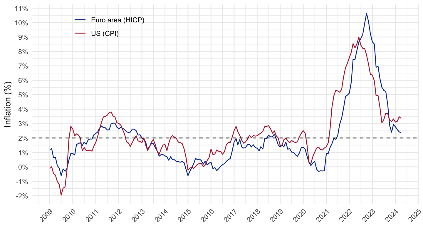
CPI, PCE, HICP
Since 2021
Inflation (1st difference, 1 year)
English
Code
Sys.setlocale("LC_TIME", "en_CA.UTF-8")# [1] "en_CA.UTF-8"Code
inflation %>%
  filter(variable %in% c("CPIAUCSL", "PCEPI", "CP0000USM086NEST", "CP00MI15EA20M086NEST")) %>%
  select(date, variable, value) %>%
  group_by(variable) %>%
  arrange(date) %>%
  mutate(value = value/lag(value, 12) - 1) %>%
  filter(date >= as.Date("2020-02-01")) %>%
  mutate(country = ifelse(variable == "CP00MI15EA20M086NEST", "Euro area", "US"),
         type = case_when(variable %in% c("CP00MI15EA20M086NEST", "CP0000USM086NEST") ~ "HICP, Proxy-HICP",
                          variable == "CPIAUCSL" ~ "CPI",
                          variable == "PCEPI" ~ "PCE"),
         type = factor(type,
                       levels  = c("HICP, Proxy-HICP", "CPI", "PCE"),
                       labels = c("Harmonized Index of Consumer Prices (HICP)",
                                        "Consumer Price Index, BLS (CPI)",
                                        "Personal Consumption Expenditures, BEA (PCE)"))) %>%
  na.omit %>%
  ggplot(.) + geom_line(aes(x = date, y = value, color = country, linetype = type)) + theme_minimal() +
  scale_x_date(breaks = seq.Date(from = as.Date("2020-01-01"), to = Sys.Date(), by = "2 months"),
               labels = date_format("%b %Y")) +
  scale_y_continuous(breaks = 0.01*seq(-60, 60, 1),
                     labels = scales::percent_format(accuracy = 1)) +
  scale_color_manual(values = c("#003399", "#B22234")) +
  xlab("") + ylab("Inflation (%)") +
  theme(legend.position = c(0.25, 0.78),
        legend.title = element_blank(),
        axis.text.x = element_text(angle = 45, vjust = 1, hjust = 1)) +
  geom_text_repel(data = . %>% filter(date %in% c(max(date), as.Date("2022-06-01"), as.Date("2022-10-01"))),
                  aes(x = date, y = value, label = percent(value, acc = 0.1)),
                  fontface ="plain", color = "black", size = 3) +
  geom_vline(xintercept = as.Date("2022-06-01"), linetype = "dotted") +
  geom_vline(xintercept = as.Date("2022-10-01"), linetype = "dotted")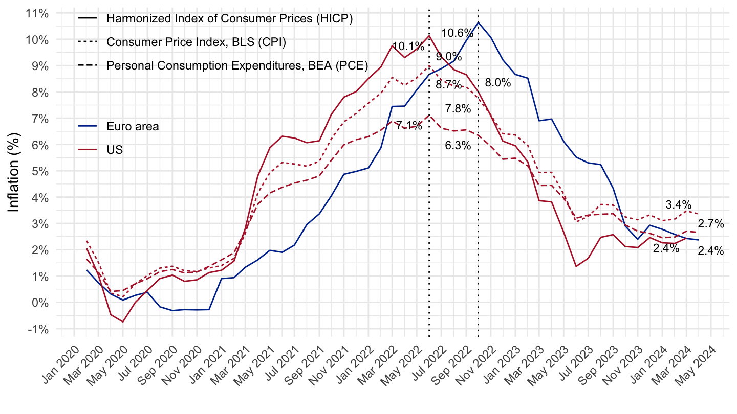
Since 2020
Inflation (1st difference, 1 year)
English
Code
inflation %>%
  filter(variable %in% c("CPIAUCSL", "PCEPI", "CP0000USM086NEST", "CP00MI15EA20M086NEST")) %>%
  select(date, variable, value) %>%
  group_by(variable) %>%
  arrange(date) %>%
  mutate(value = value/lag(value, 12) - 1) %>%
  filter(date >= as.Date("2020-01-01")) %>%
  mutate(country = ifelse(variable == "CP00MI15EA20M086NEST", "Euro area", "US"),
         type = case_when(variable %in% c("CP00MI15EA20M086NEST", "CP0000USM086NEST") ~ "Harmonized Index of Consumer Prices (HICP, Proxy-HICP)",
                          variable == "CPIAUCSL" ~ "Consumer Price Index, BLS (CPI)",
                          variable == "PCEPI" ~ "Personal Consumption Expenditures, BEA (PCE)"),
         type = factor(type, levels = c("Harmonized Index of Consumer Prices (HICP, Proxy-HICP)",
                                        "Consumer Price Index, BLS (CPI)",
                                        "Personal Consumption Expenditures, BEA (PCE)"))) %>%
  na.omit %>%
  ggplot(.) + geom_line(aes(x = date, y = value, color = country, linetype = type)) + theme_minimal() +
  scale_x_date(breaks = seq.Date(from = as.Date("2020-01-01"), to = Sys.Date(), by = "2 months"),
               labels = date_format("%b %Y")) +
  scale_y_continuous(breaks = 0.01*seq(-60, 60, 1),
                     labels = scales::percent_format(accuracy = 1)) +
  scale_color_manual(values = c("#003399", "#B22234")) +
  xlab("") + ylab("Inflation (%)") +
  theme(legend.position = c(0.3, 0.78),
        legend.title = element_blank(),
        axis.text.x = element_text(angle = 45, vjust = 1, hjust = 1)) +
  geom_text_repel(data = . %>% filter(date %in% c(max(date), as.Date("2022-06-01"), as.Date("2022-10-01"))),
                  aes(x = date, y = value, label = percent(value, acc = 0.1)),
                  fontface ="plain", color = "black", size = 3) +
  geom_vline(xintercept = as.Date("2022-06-01"), linetype = "dotted") +
  geom_vline(xintercept = as.Date("2022-10-01"), linetype = "dotted")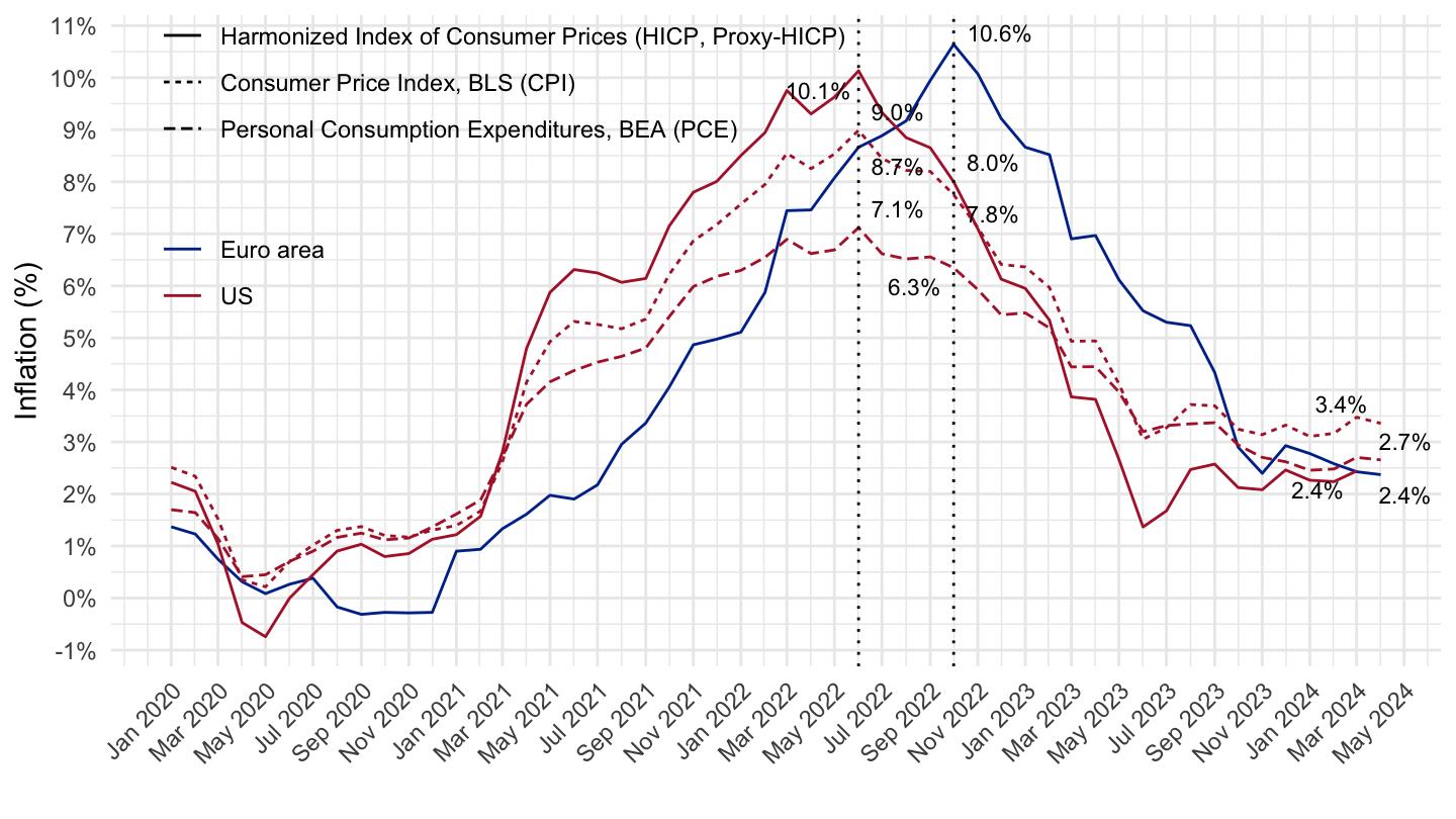
French
Code
Sys.setlocale("LC_TIME", "fr_CA.UTF-8")# [1] "fr_CA.UTF-8"Code
inflation %>%
  filter(variable %in% c("CPIAUCSL", "PCEPI", "CP0000USM086NEST", "CP00MI15EA20M086NEST")) %>%
  select(date, variable, value) %>%
  group_by(variable) %>%
  arrange(date) %>%
  mutate(value = value/lag(value, 12) - 1) %>%
  filter(date >= as.Date("2020-01-01")) %>%
  mutate(country = ifelse(variable == "CP00MI15EA20M086NEST", "Zone euro", "États-Unis"),
         country = factor(country, levels = c("Zone euro", "États-Unis")),
         type = case_when(variable %in% c("CP00MI15EA20M086NEST", "CP0000USM086NEST") ~ "Indice des Prix à la Consommation Harmonisé (IPCH, Proxy-IPCH)",
                          variable == "CPIAUCSL" ~ "Indice des Prix à la Consommation (CPI)",
                          variable == "PCEPI" ~ "Déflateur de la Consommation (PCE)"),
         type = factor(type, levels = c("Indice des Prix à la Consommation Harmonisé (IPCH, Proxy-IPCH)",
                                        "Indice des Prix à la Consommation (CPI)",
                                        "Déflateur de la Consommation (PCE)"))) %>%
  na.omit %>%
  ggplot(.) + geom_line(aes(x = date, y = value, linetype = type, color = country)) + theme_minimal() +
  scale_x_date(breaks = seq.Date(from = as.Date("2020-01-01"), to = Sys.Date(), by = "3 months"),
               labels = date_format("%b %Y")) +
  scale_y_continuous(breaks = 0.01*seq(-60, 60, 1),
                     labels = scales::percent_format(accuracy = 1)) +
  scale_color_manual(values = c("#003399", "#B22234")) +
  xlab("") + ylab("Inflation sur un an (%)") +
  theme(legend.position = c(0.3, 0.78),
        legend.title = element_blank(),
        axis.text.x = element_text(angle = 45, vjust = 1, hjust = 1)) +
  geom_text(data = . %>% filter(date %in% c(as.Date("2022-06-01"), as.Date("2022-10-01"))),
                  aes(x = date, y = value, label = percent(value, acc = 0.1)),
                  fontface ="plain", color = "black", size = 3) +
  geom_text_repel(data = . %>% filter(date %in% c(max(date))),
                  aes(x = date, y = value, label = percent(value, acc = 0.1)),
                  fontface ="plain", color = "black", size = 3) +
  geom_vline(xintercept = as.Date("2022-06-01"), linetype = "dotted") +
  geom_vline(xintercept = as.Date("2022-10-01"), linetype = "dotted") +
  guides(linetype = guide_legend(order = 1),
         color = guide_legend(order = 2))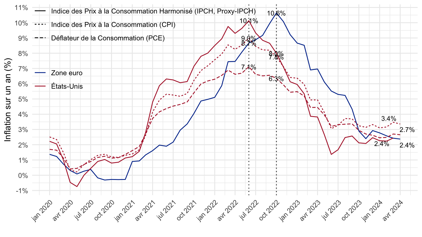
Inflation, 1st difference
1 month
Code
Sys.setlocale("LC_TIME", "en_CA.UTF-8")# [1] "en_CA.UTF-8"Code
inflation %>%
  filter(variable %in% c("CPIAUCSL", "PCEPI", "CP0000USM086NEST", "CP00MI15EA20M086NEST")) %>%
  select(date, variable, value) %>%
  group_by(variable) %>%
  arrange(date) %>%
  mutate(value = value/lag(value, 1) - 1) %>%
  filter(date >= as.Date("2020-01-01")) %>%
  mutate(country = ifelse(variable == "CP00MI15EA20M086NEST", "Euro area", "U.S."),
         type = case_when(variable %in% c("CP00MI15EA20M086NEST", "CP0000USM086NEST") ~ "Harmonized Index of Consumer Prices (HICP, Proxy-HICP)",
                          variable == "CPIAUCSL" ~ "Consumer Price Index, BLS (CPI)",
                          variable == "PCEPI" ~ "Personal Consumption Expenditures, BEA (PCE)"),
         type = factor(type, levels = c("Harmonized Index of Consumer Prices (HICP, Proxy-HICP)",
                                        "Consumer Price Index, BLS (CPI)",
                                        "Personal Consumption Expenditures, BEA (PCE)"))) %>%
  na.omit %>%
  ggplot(.) + geom_line(aes(x = date, y = value, color = country, linetype = type)) + theme_minimal() +
  scale_x_date(breaks = seq.Date(from = as.Date("2020-01-01"), to = Sys.Date(), by = "2 months"),
               labels = date_format("%b %Y")) +
  scale_y_continuous(breaks = 0.01*seq(-60, 60, 1),
                     labels = scales::percent_format(accuracy = 1)) +
  scale_color_manual(values = c("#003399", "#B22234")) +
  xlab("") + ylab("Inflation, 1 month (%)") +
  theme(legend.position = c(0.3, 0.78),
        legend.title = element_blank(),
        axis.text.x = element_text(angle = 45, vjust = 1, hjust = 1)) +
  geom_text(data = . %>% filter(date %in% c(max(date), as.Date("2022-06-01"), as.Date("2022-10-01"))),
                  aes(x = date, y = value, label = percent(value, acc = 0.1)),
                  fontface ="plain", color = "black", size = 3) +
  geom_vline(xintercept = as.Date("2022-06-01"), linetype = "dotted") +
  geom_vline(xintercept = as.Date("2022-10-01"), linetype = "dotted")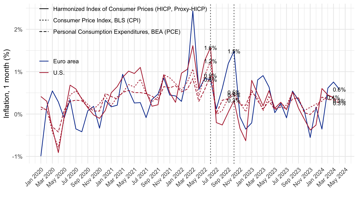
2 months
Code
inflation %>%
  filter(variable %in% c("CPIAUCSL", "PCEPI", "CP0000USM086NEST", "CP00MI15EA20M086NEST")) %>%
  select(date, variable, value) %>%
  group_by(variable) %>%
  arrange(date) %>%
  mutate(value = value/lag(value, 2) - 1) %>%
  filter(date >= as.Date("2020-01-01")) %>%
  mutate(country = ifelse(variable == "CP00MI15EA20M086NEST", "Euro area", "U.S."),
         type = case_when(variable %in% c("CP00MI15EA20M086NEST", "CP0000USM086NEST") ~ "Harmonized Index of Consumer Prices (HICP, Proxy-HICP)",
                          variable == "CPIAUCSL" ~ "Consumer Price Index, BLS (CPI)",
                          variable == "PCEPI" ~ "Personal Consumption Expenditures, BEA (PCE)"),
         type = factor(type, levels = c("Harmonized Index of Consumer Prices (HICP, Proxy-HICP)",
                                        "Consumer Price Index, BLS (CPI)",
                                        "Personal Consumption Expenditures, BEA (PCE)"))) %>%
  na.omit %>%
  ggplot(.) + geom_line(aes(x = date, y = value, color = country, linetype = type)) + theme_minimal() +
  scale_x_date(breaks = seq.Date(from = as.Date("2020-01-01"), to = Sys.Date(), by = "2 months"),
               labels = date_format("%b %Y")) +
  scale_y_continuous(breaks = 0.01*seq(-60, 60, 1),
                     labels = scales::percent_format(accuracy = 1)) +
  scale_color_manual(values = c("#003399", "#B22234")) +
  xlab("") + ylab("Inflation, 2 months (%)") +
  theme(legend.position = c(0.3, 0.78),
        legend.title = element_blank(),
        axis.text.x = element_text(angle = 45, vjust = 1, hjust = 1)) +
  geom_text(data = . %>% filter(date %in% c(max(date), as.Date("2022-06-01"), as.Date("2022-10-01"))),
                  aes(x = date, y = value, label = percent(value, acc = 0.1)),
                  fontface ="plain", color = "black", size = 3) +
  geom_vline(xintercept = as.Date("2022-06-01"), linetype = "dotted") +
  geom_vline(xintercept = as.Date("2022-10-01"), linetype = "dotted")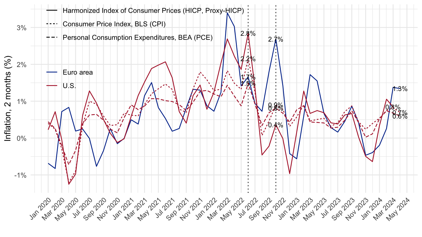
3 months
Code
inflation %>%
  filter(variable %in% c("CPIAUCSL", "PCEPI", "CP0000USM086NEST", "CP00MI15EA20M086NEST")) %>%
  select(date, variable, value) %>%
  group_by(variable) %>%
  arrange(date) %>%
  mutate(value = value/lag(value, 3) - 1) %>%
  filter(date >= as.Date("2020-01-01")) %>%
  mutate(country = ifelse(variable == "CP00MI15EA20M086NEST", "Euro area", "U.S."),
         type = case_when(variable %in% c("CP00MI15EA20M086NEST", "CP0000USM086NEST") ~ "Harmonized Index of Consumer Prices (HICP, Proxy-HICP)",
                          variable == "CPIAUCSL" ~ "Consumer Price Index, BLS (CPI)",
                          variable == "PCEPI" ~ "Personal Consumption Expenditures, BEA (PCE)"),
         type = factor(type, levels = c("Harmonized Index of Consumer Prices (HICP, Proxy-HICP)",
                                        "Consumer Price Index, BLS (CPI)",
                                        "Personal Consumption Expenditures, BEA (PCE)"))) %>%
  na.omit %>%
  ggplot(.) + geom_line(aes(x = date, y = value, color = country, linetype = type)) + theme_minimal() +
  scale_x_date(breaks = seq.Date(from = as.Date("2020-01-01"), to = Sys.Date(), by = "2 months"),
               labels = date_format("%b %Y")) +
  scale_y_continuous(breaks = 0.01*seq(-60, 60, 1),
                     labels = scales::percent_format(accuracy = 1)) +
  scale_color_manual(values = c("#003399", "#B22234")) +
  xlab("") + ylab("Inflation, 3 months (%)") +
  theme(legend.position = c(0.3, 0.78),
        legend.title = element_blank(),
        axis.text.x = element_text(angle = 45, vjust = 1, hjust = 1)) +
  geom_text(data = . %>% filter(date %in% c(max(date), as.Date("2022-06-01"), as.Date("2022-10-01"))),
                  aes(x = date, y = value, label = percent(value, acc = 0.1)),
                  fontface ="plain", color = "black", size = 3) +
  geom_vline(xintercept = as.Date("2022-06-01"), linetype = "dotted") +
  geom_vline(xintercept = as.Date("2022-10-01"), linetype = "dotted")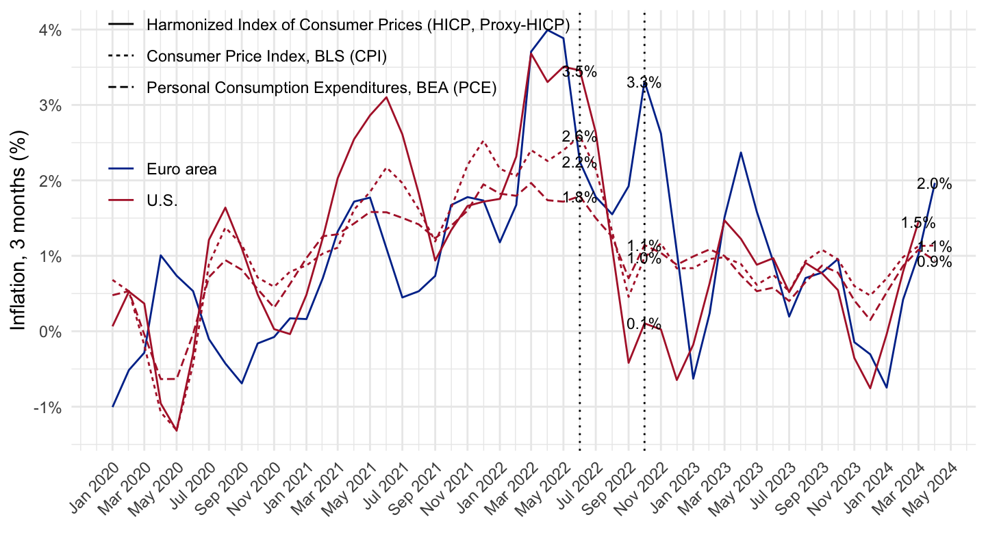
6 months
Code
inflation %>%
  filter(variable %in% c("CPIAUCSL", "PCEPI", "CP0000USM086NEST", "CP00MI15EA20M086NEST")) %>%
  select(date, variable, value) %>%
  group_by(variable) %>%
  arrange(date) %>%
  mutate(value = value/lag(value, 6) - 1) %>%
  filter(date >= as.Date("2020-01-01")) %>%
  mutate(country = ifelse(variable == "CP00MI15EA20M086NEST", "Euro area", "U.S."),
         type = case_when(variable %in% c("CP00MI15EA20M086NEST", "CP0000USM086NEST") ~ "Harmonized Index of Consumer Prices (HICP, Proxy-HICP)",
                          variable == "CPIAUCSL" ~ "Consumer Price Index, BLS (CPI)",
                          variable == "PCEPI" ~ "Personal Consumption Expenditures, BEA (PCE)"),
         type = factor(type, levels = c("Harmonized Index of Consumer Prices (HICP, Proxy-HICP)",
                                        "Consumer Price Index, BLS (CPI)",
                                        "Personal Consumption Expenditures, BEA (PCE)"))) %>%
  na.omit %>%
  ggplot(.) + geom_line(aes(x = date, y = value, color = country, linetype = type)) + theme_minimal() +
  scale_x_date(breaks = seq.Date(from = as.Date("2020-01-01"), to = Sys.Date(), by = "2 months"),
               labels = date_format("%b %Y")) +
  scale_y_continuous(breaks = 0.01*seq(-60, 60, 1),
                     labels = scales::percent_format(accuracy = 1)) +
  scale_color_manual(values = c("#003399", "#B22234")) +
  xlab("") + ylab("Inflation, 6 months (%)") +
  theme(legend.position = c(0.3, 0.78),
        legend.title = element_blank(),
        axis.text.x = element_text(angle = 45, vjust = 1, hjust = 1)) +
  geom_text(data = . %>% filter(date %in% c(max(date), as.Date("2022-06-01"), as.Date("2022-10-01"))),
                  aes(x = date, y = value, label = percent(value, acc = 0.1)),
                  fontface ="plain", color = "black", size = 3) +
  geom_vline(xintercept = as.Date("2022-06-01"), linetype = "dotted") +
  geom_vline(xintercept = as.Date("2022-10-01"), linetype = "dotted")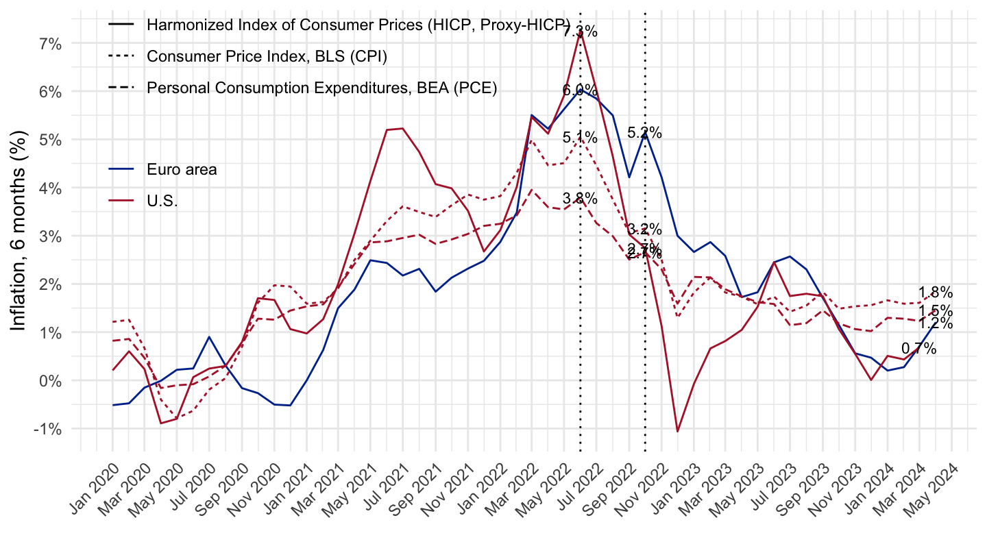
Price Index
English
Code
inflation %>%
  filter(variable %in% c("CPIAUCSL", "PCEPI", "CP0000USM086NEST", "CP00MI15EA20M086NEST")) %>%
  add_row(date = as.Date("2023-10-01"), variable = "CP00MI15EA20M086NEST", value = 124.55) %>%
  select(date, variable, value) %>%
  filter(date >= as.Date("2020-01-01")) %>%
  group_by(variable) %>%
  arrange(date) %>%
  mutate(value = 100*value/value[1]) %>%
  mutate(country = ifelse(variable == "CP00MI15EA20M086NEST", "Euro area", "US"),
         type = case_when(variable %in% c("CP00MI15EA20M086NEST", "CP0000USM086NEST") ~ "Harmonized Index of Consumer Prices (HICP, Proxy-HICP)",
                          variable == "CPIAUCSL" ~ "Consumer Price Index, BLS (CPI)",
                          variable == "PCEPI" ~ "Personal Consumption Expenditures, BEA (PCE)"),
         type = factor(type, levels = c("Harmonized Index of Consumer Prices (HICP, Proxy-HICP)",
                                        "Consumer Price Index, BLS (CPI)",
                                        "Personal Consumption Expenditures, BEA (PCE)"))) %>%
  na.omit %>%
  ggplot(.) + geom_line(aes(x = date, y = value, color = country, linetype = type)) + theme_minimal() +
  scale_x_date(breaks = seq.Date(from = as.Date("2020-01-01"), to = Sys.Date(), by = "2 months"),
               labels = date_format("%b %Y")) +
  scale_y_continuous(breaks = seq(100, 200, 5)) +
  scale_color_manual(values = c("#003399", "#B22234")) +
  xlab("") + ylab("Price Index (January 2020 = 100)") +
  theme(legend.position = c(0.3, 0.78),
        legend.title = element_blank(),
        axis.text.x = element_text(angle = 45, vjust = 1, hjust = 1))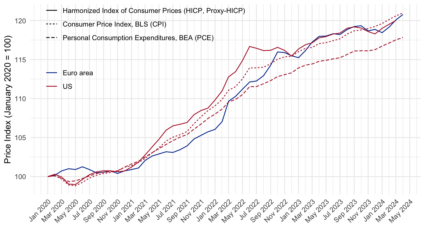
French
Code
Sys.setlocale("LC_TIME", "fr_CA.UTF-8")# [1] "fr_CA.UTF-8"Code
inflation %>%
  filter(variable %in% c("CPIAUCSL", "PCEPI", "CP0000USM086NEST", "CP00MI15EA20M086NEST")) %>%
  add_row(date = as.Date("2023-10-01"), variable = "CP00MI15EA20M086NEST", value = 124.55) %>%
  select(date, variable, value) %>%
  filter(date >= as.Date("2020-01-01")) %>%
  group_by(variable) %>%
  arrange(date) %>%
  mutate(value = 100*value/value[1]) %>%
  mutate(country = ifelse(variable == "CP00MI15EA20M086NEST", "Zone euro", "États-Unis"),
         country = factor(country, levels = c("Zone euro", "États-Unis")),
         type = case_when(variable %in% c("CP00MI15EA20M086NEST", "CP0000USM086NEST") ~ "Indice des Prix à la Consommation Harmonisé (IPCH, Proxy-IPCH)",
                          variable == "CPIAUCSL" ~ "Indice des Prix à la Consommation (CPI)",
                          variable == "PCEPI" ~ "Déflateur de la Consommation (PCE)"),
         type = factor(type, levels = c("Indice des Prix à la Consommation Harmonisé (IPCH, Proxy-IPCH)",
                                        "Indice des Prix à la Consommation (CPI)",
                                        "Déflateur de la Consommation (PCE)"))) %>%
  na.omit %>%
  ggplot(.) + geom_line(aes(x = date, y = value, color = country, linetype = type)) + theme_minimal() +
  scale_x_date(breaks = seq.Date(from = as.Date("2020-01-01"), to = Sys.Date(), by = "3 months"),
               labels = date_format("%b %Y")) +
  scale_y_continuous(breaks = seq(100, 200, 5)) +
  scale_color_manual(values = c("#003399", "#B22234")) +
  xlab("") + ylab("Indice des prix (Janvier 2020 = 100)") +
  theme(legend.position = c(0.3, 0.78),
        legend.title = element_blank(),
        axis.text.x = element_text(angle = 45, vjust = 1, hjust = 1)) +
  guides(linetype = guide_legend(order = 1),
         color = guide_legend(order = 2))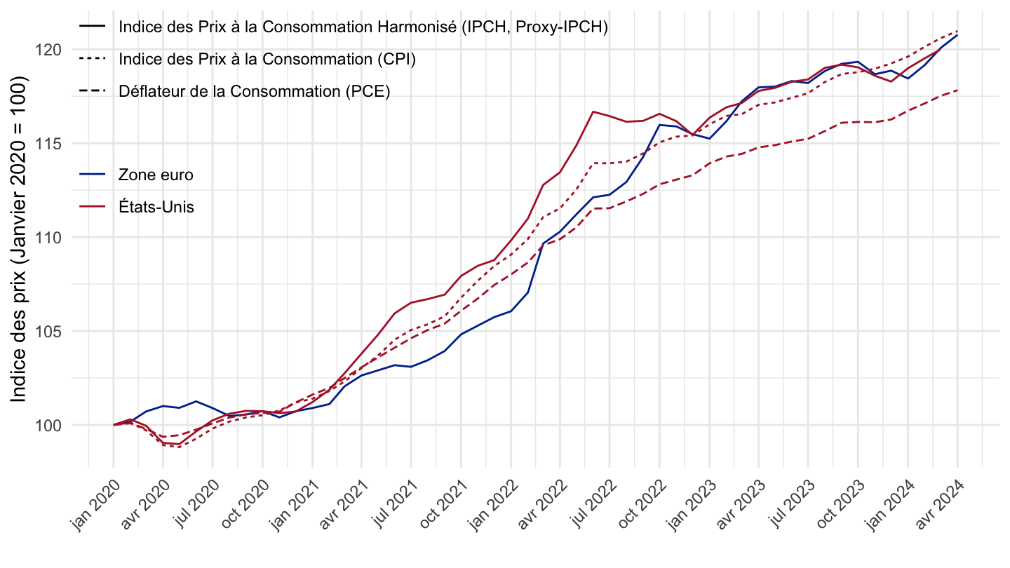
Code
Sys.setlocale("LC_TIME", "en_CA.UTF-8")# [1] "en_CA.UTF-8"Core CPI, PCE, HICP
Since 2020
Inflation (1st difference)
1 year
Code
inflation %>%
  filter(variable %in% c("PCEPILFE", "CPILFESL", "TOTNRGFOODEA20MI15XM")) %>%
  select(date, variable, value) %>%
  group_by(variable) %>%
  arrange(date) %>%
  mutate(value = value/lag(value, 12) - 1) %>%
  filter(date >= as.Date("2020-01-01")) %>%
  mutate(country = ifelse(variable == "TOTNRGFOODEA20MI15XM", "Euro area", "U.S."),
         type = case_when(variable %in% c("TOTNRGFOODEA20MI15XM") ~ "Harmonized Index of Consumer Prices (HICP)",
                          variable == "CPILFESL" ~ "Consumer Price Index, BLS (CPI)",
                          variable == "PCEPILFE" ~ "Personal Consumption Expenditures, BEA (PCE)"),
         type = factor(type, levels = c("Harmonized Index of Consumer Prices (HICP)",
                                        "Consumer Price Index, BLS (CPI)",
                                        "Personal Consumption Expenditures, BEA (PCE)"))) %>%
  na.omit %>%
  ggplot(.) + geom_line(aes(x = date, y = value, color = country, linetype = type)) + theme_minimal() +
  scale_x_date(breaks = seq.Date(from = as.Date("2020-01-01"), to = Sys.Date(), by = "2 months"),
               labels = scales::date_format("%b %Y")) +
  scale_y_continuous(breaks = 0.01*seq(-60, 60, 1),
                     labels = scales::percent_format(accuracy = 1)) +
  scale_color_manual(values = c("#003399", "#B22234")) +
  xlab("") + ylab("Core Inflation (%)") +
  theme(legend.position = c(0.25, 0.78),
        legend.title = element_blank(),
        axis.text.x = element_text(angle = 45, vjust = 1, hjust = 1)) +
  geom_text(data = . %>% filter(date %in% c(max(date), as.Date("2022-06-01"), as.Date("2022-10-01"))),
                  aes(x = date, y = value, label = scales::percent(value, acc = 0.1)),
                  fontface ="plain", color = "black", size = 3) +
  geom_vline(xintercept = as.Date("2022-06-01"), linetype = "dotted") +
  geom_vline(xintercept = as.Date("2022-10-01"), linetype = "dotted")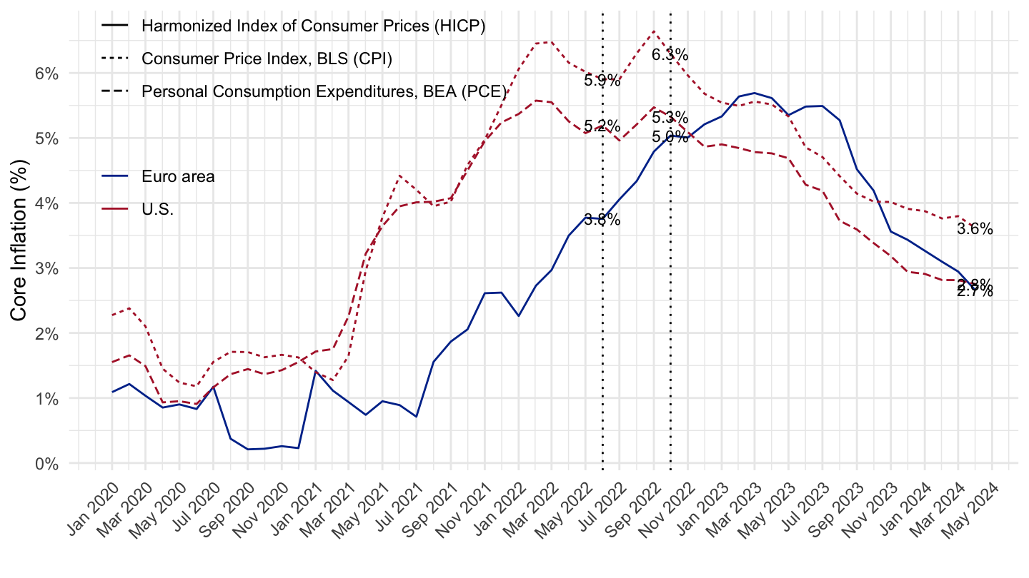
6 months
Code
inflation %>%
  filter(variable %in% c("PCEPILFE", "CPILFESL", "TOTNRGFOODEA20MI15XM")) %>%
  select(date, variable, value) %>%
  group_by(variable) %>%
  arrange(date) %>%
  mutate(value = (value/lag(value, 6))^2 - 1) %>%
  filter(date >= as.Date("2020-01-01")) %>%
  mutate(country = ifelse(variable == "TOTNRGFOODEA20MI15XM", "Euro area", "U.S."),
         type = case_when(variable %in% c("TOTNRGFOODEA20MI15XM") ~ "Harmonized Index of Consumer Prices (HICP)",
                          variable == "CPILFESL" ~ "Consumer Price Index, BLS (CPI)",
                          variable == "PCEPILFE" ~ "Personal Consumption Expenditures, BEA (PCE)"),
         type = factor(type, levels = c("Harmonized Index of Consumer Prices (HICP)",
                                        "Consumer Price Index, BLS (CPI)",
                                        "Personal Consumption Expenditures, BEA (PCE)"))) %>%
  na.omit %>%
  ggplot(.) + geom_line(aes(x = date, y = value, color = country, linetype = type)) + theme_minimal() +
  scale_x_date(breaks = seq.Date(from = as.Date("2020-01-01"), to = Sys.Date(), by = "2 months"),
               labels = scales::date_format("%b %Y")) +
  scale_y_continuous(breaks = 0.01*seq(-60, 60, 1),
                     labels = scales::percent_format(accuracy = 1)) +
  scale_color_manual(values = c("#003399", "#B22234")) +
  xlab("") + ylab("Core Inflation, 6 months annualized (%)") +
  theme(legend.position = c(0.25, 0.78),
        legend.title = element_blank(),
        axis.text.x = element_text(angle = 45, vjust = 1, hjust = 1)) +
  geom_text(data = . %>% filter(date %in% c(max(date), as.Date("2022-06-01"), as.Date("2022-10-01"))),
                  aes(x = date, y = value, label = scales::percent(value, acc = 0.1)),
                  fontface ="plain", color = "black", size = 3)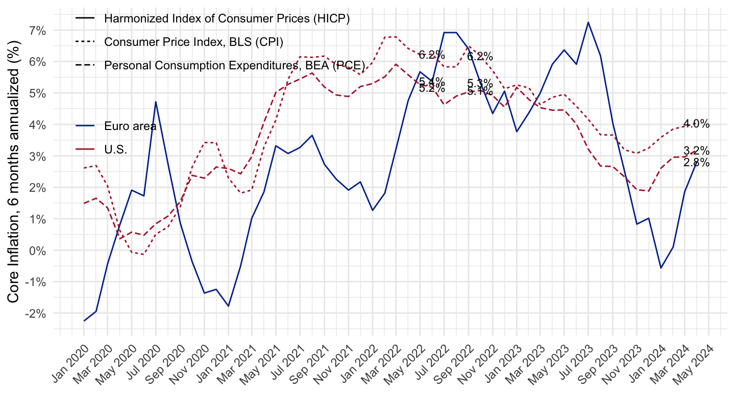
3 months
Code
inflation %>%
  filter(variable %in% c("PCEPILFE", "CPILFESL", "TOTNRGFOODEA20MI15XM")) %>%
  select(date, variable, value) %>%
  group_by(variable) %>%
  arrange(date) %>%
  mutate(value = (value/lag(value, 3))^4 - 1) %>%
  filter(date >= as.Date("2020-01-01")) %>%
  mutate(country = ifelse(variable == "TOTNRGFOODEA20MI15XM", "Euro area", "U.S."),
         type = case_when(variable %in% c("TOTNRGFOODEA20MI15XM") ~ "Harmonized Index of Consumer Prices (HICP)",
                          variable == "CPILFESL" ~ "Consumer Price Index, BLS (CPI)",
                          variable == "PCEPILFE" ~ "Personal Consumption Expenditures, BEA (PCE)"),
         type = factor(type, levels = c("Harmonized Index of Consumer Prices (HICP)",
                                        "Consumer Price Index, BLS (CPI)",
                                        "Personal Consumption Expenditures, BEA (PCE)"))) %>%
  na.omit %>%
  ggplot(.) + geom_line(aes(x = date, y = value, color = country, linetype = type)) + theme_minimal() +
  scale_x_date(breaks = seq.Date(from = as.Date("2020-01-01"), to = Sys.Date(), by = "2 months"),
               labels = scales::date_format("%b %Y")) +
  scale_y_continuous(breaks = 0.01*seq(-60, 60, 1),
                     labels = scales::percent_format(accuracy = 1)) +
  scale_color_manual(values = c("#003399", "#B22234")) +
  xlab("") + ylab("Core Inflation, 3 months annualized (%)") +
  theme(legend.position = c(0.25, 0.78),
        legend.title = element_blank(),
        axis.text.x = element_text(angle = 45, vjust = 1, hjust = 1)) +
  geom_text(data = . %>% filter(date %in% c(max(date), as.Date("2022-06-01"), as.Date("2022-10-01"))),
                  aes(x = date, y = value, label = scales::percent(value, acc = 0.1)),
                  fontface ="plain", color = "black", size = 3)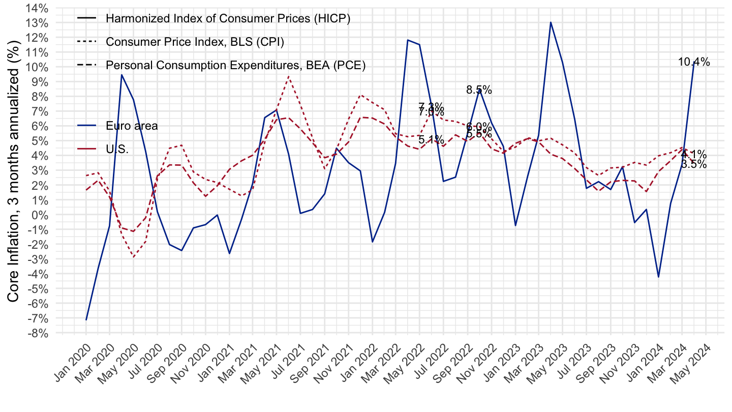
Price Index
Code
inflation %>%
  filter(variable %in% c("PCEPILFE", "CPILFESL", "TOTNRGFOODEA20MI15XM")) %>%
  select(date, variable, value) %>%
  filter(date >= as.Date("2020-01-01")) %>%
  group_by(variable) %>%
  arrange(date) %>%
  mutate(value = 100*value/value[1]) %>%
  mutate(country = ifelse(variable == "TOTNRGFOODEA20MI15XM", "Euro area", "U.S."),
         type = case_when(variable %in% c("TOTNRGFOODEA20MI15XM") ~ "Harmonized Index of Consumer Prices (HICP)",
                          variable == "CPILFESL" ~ "Consumer Price Index, BLS (CPI)",
                          variable == "PCEPILFE" ~ "Personal Consumption Expenditures, BEA (PCE)"),
         type = factor(type, levels = c("Harmonized Index of Consumer Prices (HICP)",
                                        "Consumer Price Index, BLS (CPI)",
                                        "Personal Consumption Expenditures, BEA (PCE)"))) %>%
  na.omit %>%
  ggplot(.) + geom_line(aes(x = date, y = value, color = country, linetype = type)) + theme_minimal() +
  scale_x_date(breaks = seq.Date(from = as.Date("2020-01-01"), to = Sys.Date(), by = "2 months"),
               labels = scales::date_format("%b %Y")) +
  scale_y_continuous(breaks = seq(100, 200, 5)) +
  scale_color_manual(values = c("#003399", "#B22234")) +
  xlab("") + ylab("Price Index (January 2020 = 100)") +
  theme(legend.position = c(0.3, 0.78),
        legend.title = element_blank(),
        axis.text.x = element_text(angle = 45, vjust = 1, hjust = 1))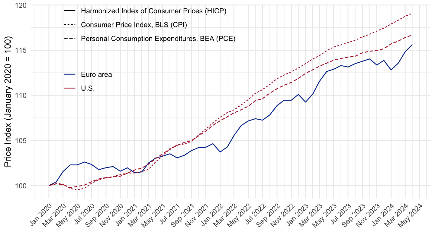
Since 2021
Inflation (1st difference)
3 months
Code
inflation %>%
  filter(variable %in% c("CPILFESL", "TOTNRGFOODEA20MI15XM")) %>%
  select(date, variable, value) %>%
  group_by(variable) %>%
  arrange(date) %>%
  mutate(value = (value/lag(value, 3))^4 - 1) %>%
  filter(date >= as.Date("2022-01-01")) %>%
  mutate(country = ifelse(variable == "TOTNRGFOODEA20MI15XM", "Euro area", "U.S."),
         type = case_when(variable %in% c("TOTNRGFOODEA20MI15XM") ~ "Harmonized Index of Consumer Prices (HICP)",
                          variable == "CPILFESL" ~ "Consumer Price Index, BLS (CPI)",
                          variable == "PCEPILFE" ~ "Personal Consumption Expenditures, BEA (PCE)"),
         type = factor(type, levels = c("Harmonized Index of Consumer Prices (HICP)",
                                        "Consumer Price Index, BLS (CPI)",
                                        "Personal Consumption Expenditures, BEA (PCE)"))) %>%
  na.omit %>%
  ggplot(.) + geom_line(aes(x = date, y = value, color = country)) + theme_minimal() +
  scale_x_date(breaks = seq.Date(from = as.Date("2020-01-01"), to = Sys.Date(), by = "2 months"),
               labels = scales::date_format("%b %Y")) +
  scale_y_continuous(breaks = 0.01*seq(-60, 60, 1),
                     labels = scales::percent_format(accuracy = 1)) +
  scale_color_manual(values = c("#003399", "#B22234")) +
  xlab("") + ylab("Core Inflation, 3 months annualized (%)") +
  theme(legend.position = c(0.25, 0.78),
        legend.title = element_blank(),
        axis.text.x = element_text(angle = 45, vjust = 1, hjust = 1)) +
  geom_text(aes(x = date, y = value, label = scales::percent(value, acc = 0.1)),
                  fontface ="plain", color = "black", size = 3)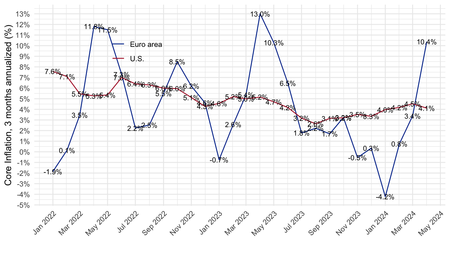
CPi, PCE, PCE without energy and food
2010-
Code
inflation %>%
  filter(variable %in% c("CPIAUCSL", "PCEPI", "PCEPILFE", "CPILFESL"),
         date >= as.Date("2010-01-01")) %>%
  select(date, variable, value) %>%
  group_by(variable) %>%
  arrange(date) %>%
  mutate(value = ifelse(variable == "UNRATE", value/100, value/lag(value, 12) - 1)) %>%
  left_join(variable, by = "variable") %>%
  filter(date >= as.Date("2011-01-01")) %>%
  na.omit %>%
  mutate(Variable = gsub("Consumer Price Index for All Urban Consumers", "CPI", Variable)) %>%
  ggplot(.) + geom_line(aes(x = date, y = value, color = Variable)) + theme_minimal() +
  scale_x_date(breaks = seq(1870, 2100, 1) %>% paste0("-01-01") %>% as.Date,
               labels = date_format("%Y")) +
  scale_y_continuous(breaks = 0.01*seq(-60, 60, 1),
                     labels = scales::percent_format(accuracy = 1)) +
  xlab("") + ylab("Inflation (%)") +
  theme(legend.position = c(0.4, 0.85),
        legend.title = element_blank())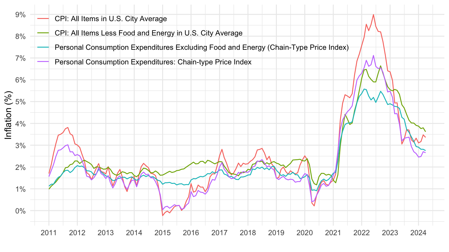
2019-
Code
inflation %>%
  filter(variable %in% c("CPIAUCSL", "PCEPI", "PCEPILFE", "CPILFESL"),
         date >= as.Date("2010-01-01")) %>%
  select(date, variable, value) %>%
  group_by(variable) %>%
  arrange(date) %>%
  mutate(value = ifelse(variable == "UNRATE", value/100, value/lag(value, 12) - 1)) %>%
  left_join(variable, by = "variable") %>%
  filter(date >= as.Date("2019-01-01")) %>%
  na.omit %>%
  mutate(Variable = gsub("Consumer Price Index for All Urban Consumers", "CPI", Variable)) %>%
  ggplot(.) + geom_line(aes(x = date, y = value, color = Variable)) + theme_minimal() +
  scale_x_date(breaks = seq(1870, 2100, 1) %>% paste0("-01-01") %>% as.Date,
               labels = date_format("%Y")) +
  scale_y_continuous(breaks = 0.01*seq(-60, 60, 1),
                     labels = scales::percent_format(accuracy = 1)) +
  xlab("") + ylab("Inflation (%)") +
  theme(legend.position = c(0.4, 0.85),
        legend.title = element_blank())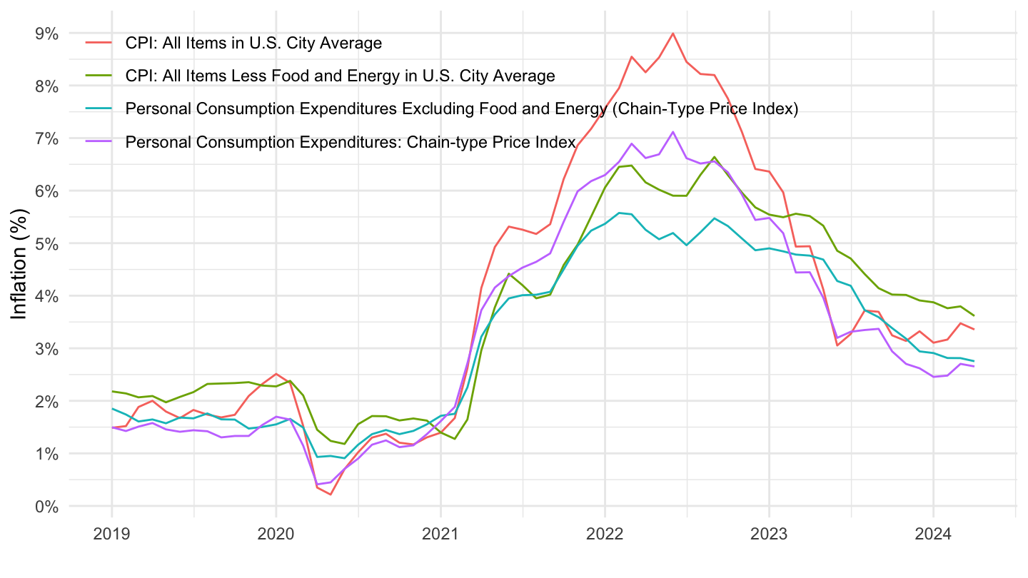
Since 2020
All
Code
inflation %>%
  filter(variable %in% c("CPIAUCSL", "PCEPI", "PCEPILFE", "CPILFESL")) %>%
  select(date, variable, value) %>%
  group_by(variable) %>%
  arrange(date) %>%
  mutate(value = value/lag(value, 12) - 1) %>%
  filter(date >= as.Date("2020-01-01")) %>%
  left_join(variable, by = "variable") %>%
  na.omit %>%
  mutate(Variable = gsub("Consumer Price Index for All Urban Consumers", "CPI", Variable)) %>%
  ggplot(.) + geom_line(aes(x = date, y = value, color = Variable)) + theme_minimal() +
  scale_x_date(breaks = "3 months",
               labels = date_format("%b %Y")) +
  scale_y_continuous(breaks = 0.01*seq(-60, 60, 1),
                     labels = scales::percent_format(accuracy = 1)) +
  xlab("") + ylab("Inflation (%)") +
  theme(legend.position = c(0.4, 0.8),
        legend.title = element_blank(),
        axis.text.x = element_text(angle = 45, vjust = 1, hjust = 1))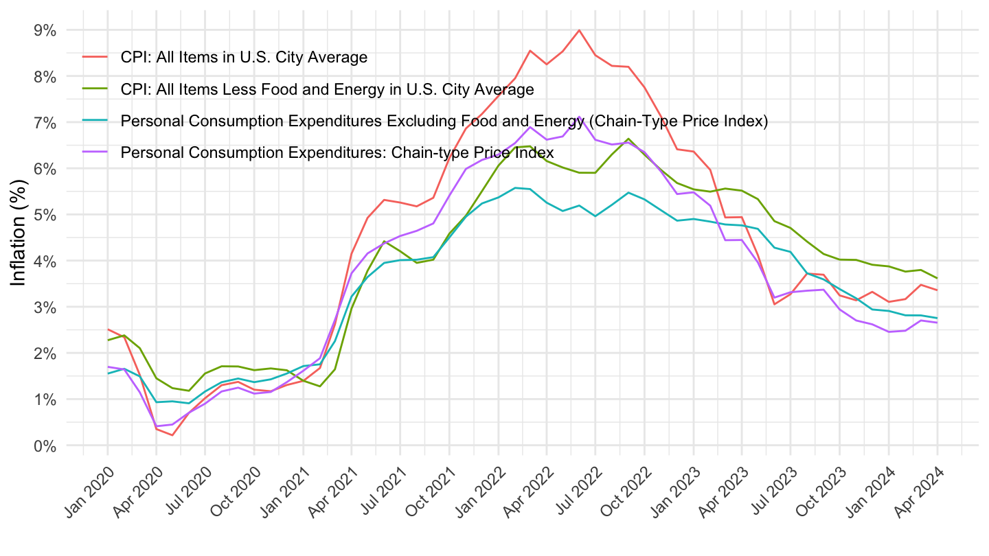
New
Code
inflation %>%
  filter(variable %in% c("CPIAUCSL", "PCEPI", "PCEPILFE", "CPILFESL")) %>%
  mutate(category = case_when(variable %in% c("PCEPI", "CPIAUCSL") ~ "All items (Headline)",
                              T ~ "All items less Food and Energy (Core)"),
         PCE_or_CPI = case_when(variable %in% c("CPIAUCSL", "CPILFESL") ~ "Consumer Price Index (CPI)",
                              T ~ "Personal Consumption Expenditures (PCE)")) %>%
  select(date, variable, value, category, PCE_or_CPI) %>%
  group_by(category, PCE_or_CPI) %>%
  arrange(date) %>%
  mutate(value = value/lag(value, 12) - 1) %>%
  filter(date >= as.Date("2020-01-01")) %>%
  na.omit %>%
  ggplot(.) + geom_line(aes(x = date, y = value, color = PCE_or_CPI, linetype = category)) + theme_minimal() +
  scale_x_date(breaks = "3 months",
               labels = date_format("%b %Y")) +
  scale_y_continuous(breaks = 0.01*seq(-60, 60, 1),
                     labels = scales::percent_format(accuracy = 1)) +
  xlab("") + ylab("US Inflation (%)") +
  theme(legend.position = c(0.25, 0.8),
        legend.title = element_blank(),
        axis.text.x = element_text(angle = 45, vjust = 1, hjust = 1))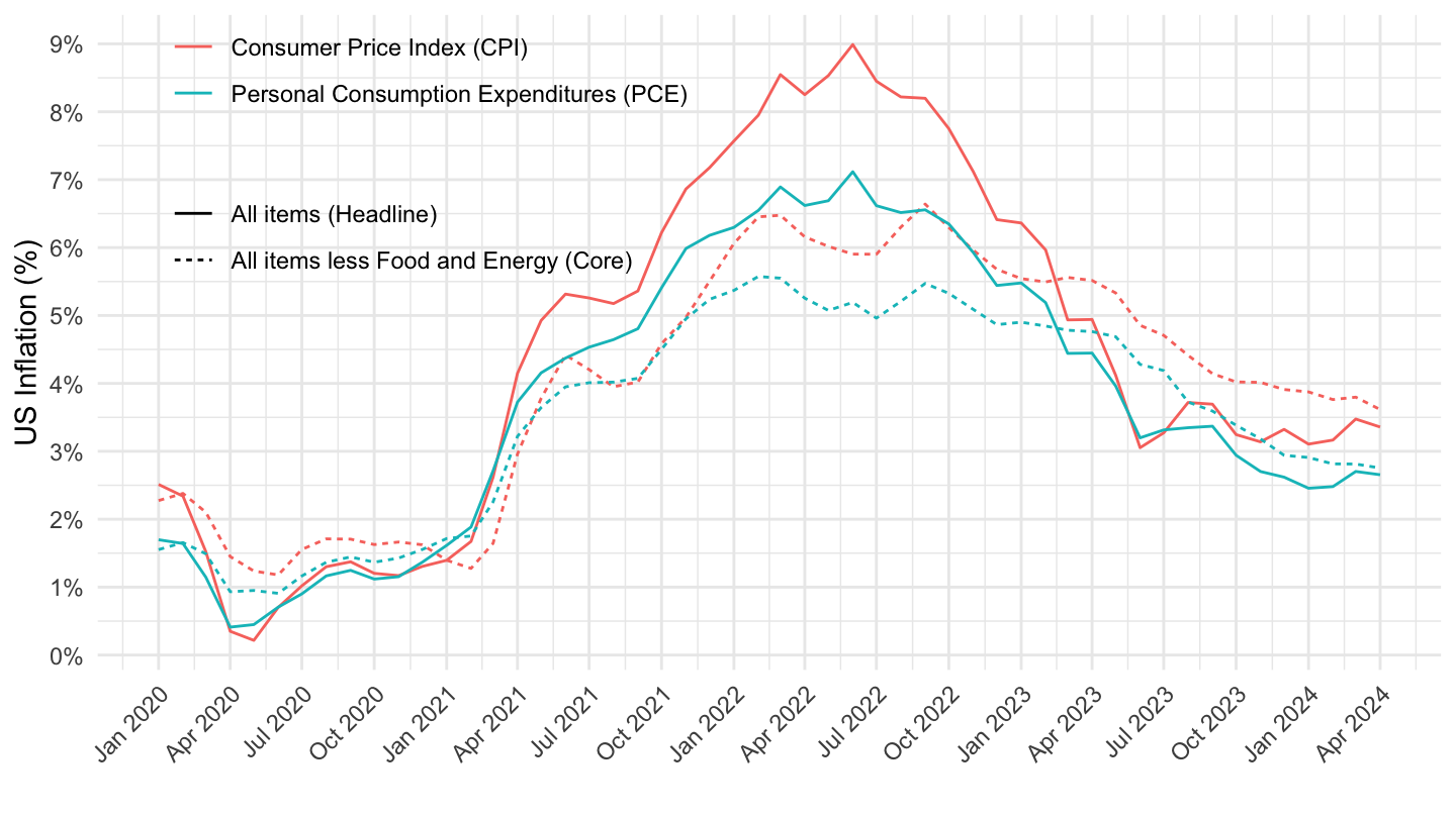
With tickers
Code
inflation %>%
  filter(variable %in% c("CPIAUCSL", "PCEPI", "PCEPILFE", "CPILFESL")) %>%
  mutate(category = case_when(variable %in% c("PCEPI", "CPIAUCSL") ~ "All items (Headline)",
                              T ~ "All items less Food and Energy (Core)"),
         PCE_or_CPI = case_when(variable %in% c("CPIAUCSL", "CPILFESL") ~ "Consumer Price Index (CPI)",
                              T ~ "Personal Consumption Expenditures (PCE)")) %>%
  select(date, variable, value, category, PCE_or_CPI) %>%
  group_by(category, PCE_or_CPI) %>%
  arrange(date) %>%
  mutate(value = value/lag(value, 12) - 1) %>%
  filter(date >= as.Date("2020-01-01")) %>%
  na.omit %>%
  ggplot(.) + geom_line(aes(x = date, y = value, color = PCE_or_CPI, linetype = category)) + theme_minimal() +
  scale_x_date(breaks = seq.Date(from = as.Date("2018-06-01"), to = Sys.Date(), by = "3 months"),
               labels = date_format("%b %Y")) +
  scale_y_continuous(breaks = 0.01*seq(-60, 60, 1),
                     labels = scales::percent_format(accuracy = 1)) +
  xlab("") + ylab("US Inflation (%)") +
  theme(legend.position = c(0.25, 0.8),
        legend.title = element_blank(),
        axis.text.x = element_text(angle = 45, vjust = 1, hjust = 1)) +
  geom_text_repel(data = . %>% filter(date %in% c(max(date), as.Date("2022-06-01"))),
                  aes(x = date, y = value, label = percent(value, acc = 0.1)),
                  fontface ="plain", color = "black", size = 3) +
  geom_vline(xintercept = as.Date("2022-06-01"), linetype = "dotted")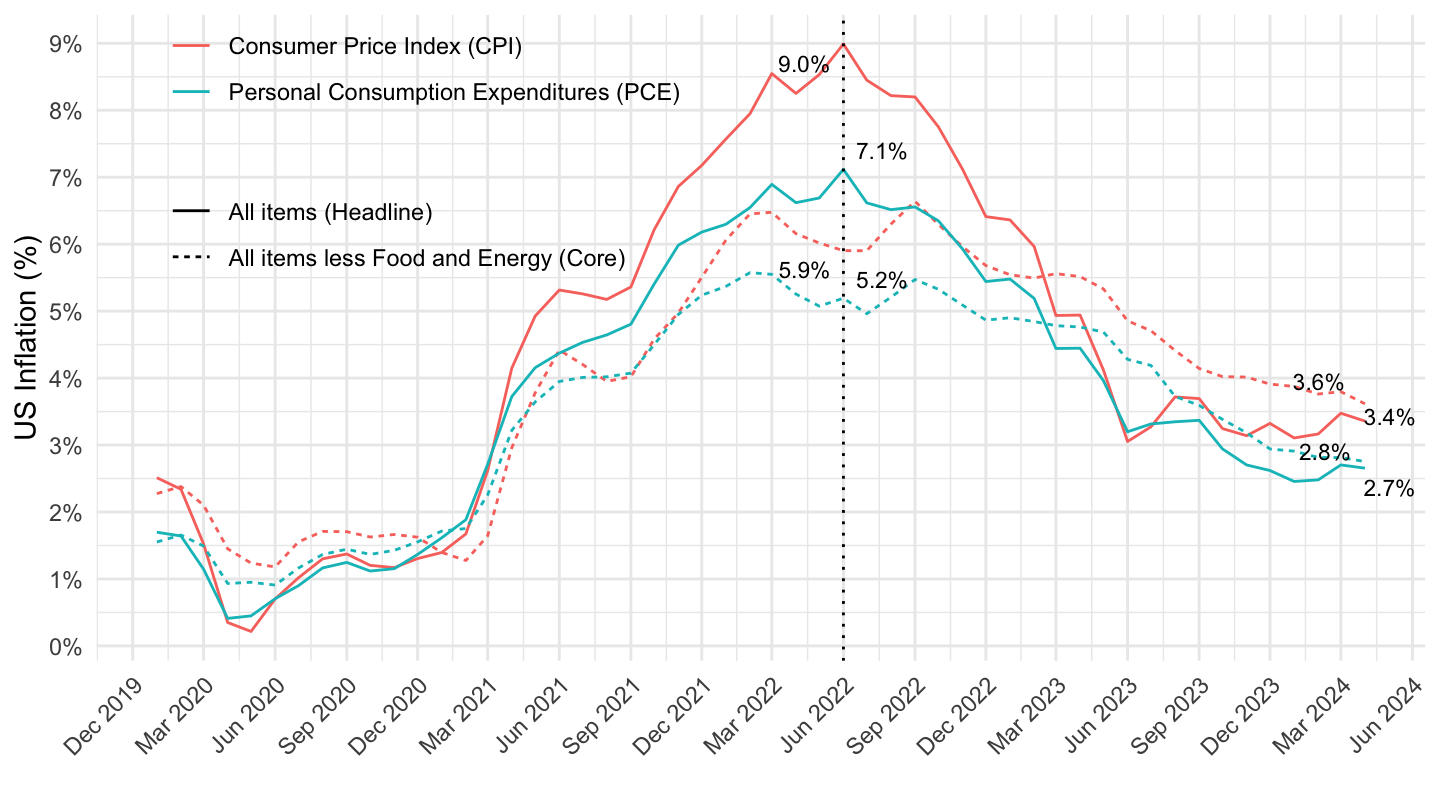
2 years
Code
inflation %>%
  filter(variable %in% c("CPIAUCSL", "PCEPI", "PCEPILFE", "CPILFESL")) %>%
  select(date, variable, value) %>%
  group_by(variable) %>%
  arrange(date) %>%
  mutate(value = value/lag(value, 12) - 1) %>%
  filter(date >= Sys.Date() - years(2)) %>%
  left_join(variable, by = "variable") %>%
  na.omit %>%
  mutate(Variable = gsub("Consumer Price Index for All Urban Consumers", "CPI", Variable)) %>%
  ggplot(.) + geom_line(aes(x = date, y = value, color = Variable)) + theme_minimal() +
  scale_x_date(breaks = "1 month",
               labels = date_format("%b %Y")) +
  scale_y_continuous(breaks = 0.01*seq(-60, 60, 1),
                     labels = scales::percent_format(accuracy = 1)) +
  xlab("") + ylab("Inflation (%)") +
  theme(legend.position = c(0.4, 0.15),
        legend.title = element_blank(),
        axis.text.x = element_text(angle = 45, vjust = 1, hjust = 1)) +
  geom_text_repel(data = . %>% filter(date %in% c(max(date), as.Date("2022-06-01"),
                                                  as.Date("2022-01-01"), as.Date("2023-02-01"))),
                  aes(x = date, y = value, label = percent(value, acc = 0.1)),
                  fontface ="plain", color = "black", size = 3) +
  geom_vline(xintercept = as.Date("2022-06-01"), linetype = "dotted") +
  geom_vline(xintercept = as.Date("2022-01-01"), linetype = "dotted") +
  geom_vline(xintercept = as.Date("2023-02-01"), linetype = "dotted")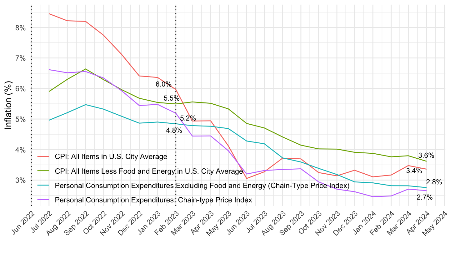
Rents,Without Rents, general, unemployment
2010-
Code
inflation %>%
  filter(variable %in% c("CPIAUCSL", "CUUR0000SA0L2", "CUUR0000SAH1", "UNRATE"),
         date >= as.Date("2010-01-01")) %>%
  select(date, variable, value) %>%
  group_by(variable) %>%
  arrange(date) %>%
  mutate(value = ifelse(variable == "UNRATE", value/100, value/lag(value, 12) - 1)) %>%
  left_join(variable, by = "variable") %>%
  filter(date >= as.Date("2011-01-01")) %>%
  na.omit %>%
  mutate(Variable = gsub("Consumer Price Index for All Urban Consumers", "CPI", Variable)) %>%
  ggplot(.) + geom_line(aes(x = date, y = value, color = Variable)) + theme_minimal() +
  scale_x_date(breaks = seq(1870, 2100, 1) %>% paste0("-01-01") %>% as.Date,
               labels = date_format("%Y")) +
  scale_y_continuous(breaks = 0.01*seq(-60, 60, 1),
                     labels = scales::percent_format(accuracy = 1)) +
  xlab("") + ylab("Inflation (%), Unemployment Rate (%)") +
  theme(legend.position = c(0.4, 0.85),
        legend.title = element_blank())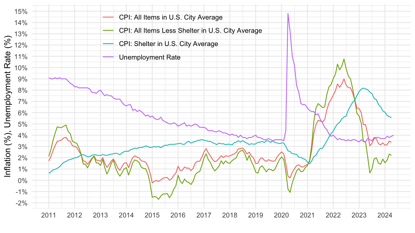
2 years
Code
inflation %>%
  filter(variable %in% c("CPIAUCSL", "CUUR0000SA0L2", "CUUR0000SAH1", "UNRATE")) %>%
  select(date, variable, value) %>%
  group_by(variable) %>%
  arrange(date) %>%
  mutate(value = ifelse(variable == "UNRATE", value/100, value/lag(value, 12) - 1)) %>%
  filter(date >= Sys.Date() - years(2)) %>%
  left_join(variable, by = "variable") %>%
  na.omit %>%
  mutate(Variable = gsub("Consumer Price Index for All Urban Consumers", "CPI", Variable)) %>%
  ggplot(.) + geom_line(aes(x = date, y = value, color = Variable)) + theme_minimal() +
  scale_x_date(breaks = "2 months",
               labels = date_format("%b %Y")) +
  scale_y_continuous(breaks = 0.01*seq(-60, 60, 1),
                     labels = scales::percent_format(accuracy = 1)) +
  xlab("") + ylab("Inflation (%), Unemployment Rate (%)") +
  theme(legend.position = c(0.3, 0.15),
        legend.title = element_blank(),
        axis.text.x = element_text(angle = 45, vjust = 1, hjust = 1))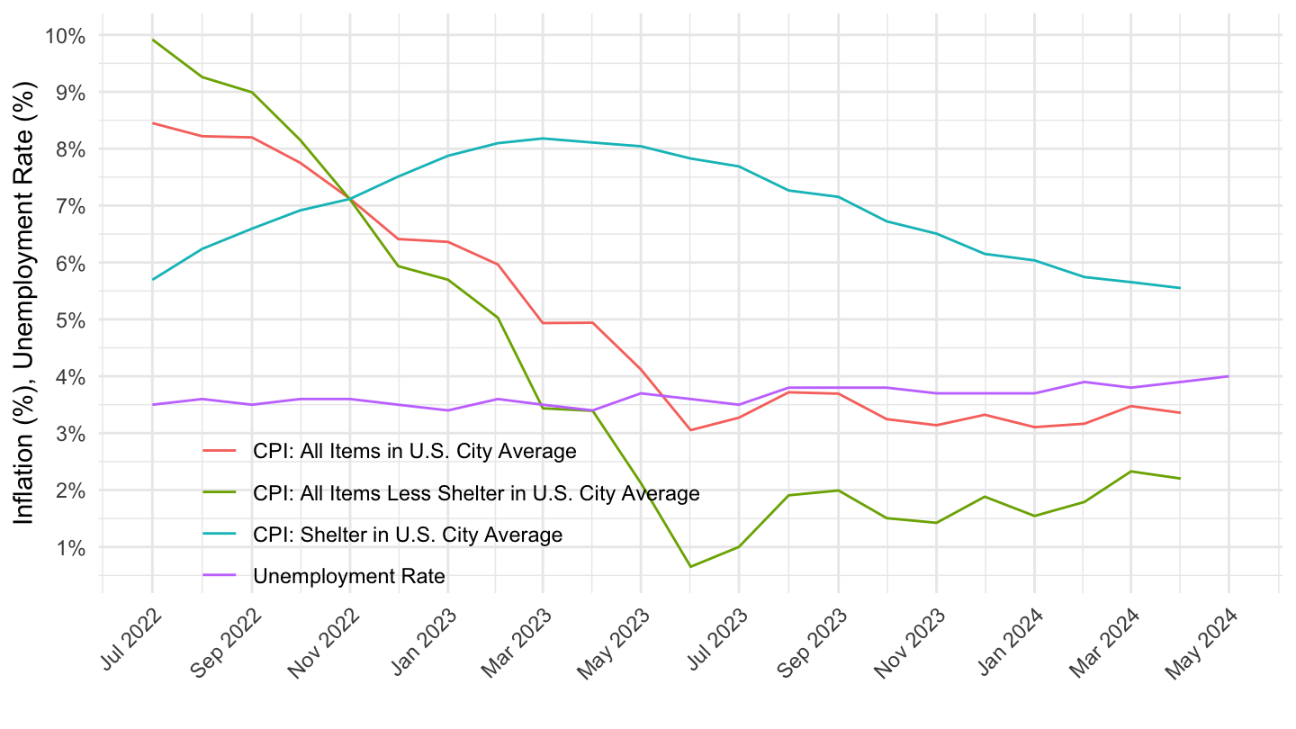
Rents,Without Rents VS general
2010-
Code
inflation %>%
  filter(variable %in% c("CPIAUCSL", "CUUR0000SA0L2", "CUUR0000SAH1"),
         date >= as.Date("2010-01-01")) %>%
  select(date, variable, value) %>%
  group_by(variable) %>%
  arrange(date) %>%
  mutate(value = value/lag(value, 12) - 1) %>%
  left_join(variable, by = "variable") %>%
  na.omit %>%
  mutate(Variable = gsub("Consumer Price Index for All Urban Consumers", "CPI", Variable)) %>%
  ggplot(.) + geom_line(aes(x = date, y = value, color = Variable)) + theme_minimal() +
  scale_x_date(breaks = seq(1870, 2100, 1) %>% paste0("-01-01") %>% as.Date,
               labels = date_format("%Y")) +
  scale_y_continuous(breaks = 0.01*seq(-60, 60, 1),
                     labels = scales::percent_format(accuracy = 1)) +
  xlab("") + ylab("Inflation (%)") +
  theme(legend.position = c(0.5, 0.9),
        legend.title = element_blank())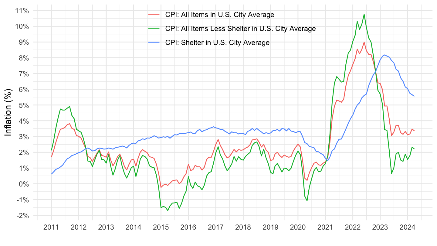
2 years
Code
inflation %>%
  filter(variable %in% c("CPIAUCSL", "CUUR0000SA0L2", "CUUR0000SAH1")) %>%
  select(date, variable, value) %>%
  group_by(variable) %>%
  arrange(date) %>%
  mutate(value = value/lag(value, 12) - 1) %>%
  filter(date >= Sys.Date() - years(3)) %>%
  left_join(variable, by = "variable") %>%
  na.omit %>%
  mutate(Variable = gsub("Consumer Price Index for All Urban Consumers", "CPI", Variable)) %>%
  ggplot(.) + geom_line(aes(x = date, y = value, color = Variable)) + theme_minimal() +
  scale_x_date(breaks = "2 months",
               labels = date_format("%b %Y")) +
  scale_y_continuous(breaks = 0.01*seq(-60, 60, 1),
                     labels = scales::percent_format(accuracy = 1)) +
  xlab("") + ylab("Inflation (%)") +
  theme(legend.position = c(0.5, 0.2),
        legend.title = element_blank(),
        axis.text.x = element_text(angle = 45, vjust = 1, hjust = 1))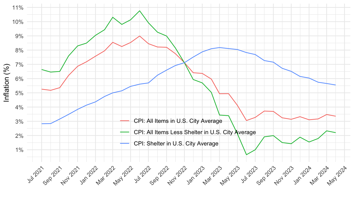
Without Rents VS general
All
Code
inflation %>%
  filter(variable %in% c("CPIAUCSL", "CUUR0000SA0L2"),
         date >= as.Date("1947-01-01")) %>%
  select(date, variable, value) %>%
  group_by(variable) %>%
  arrange(date) %>%
  mutate(value = value/lag(value, 12) - 1) %>%
  left_join(variable, by = "variable") %>%
  na.omit %>%
  mutate(Variable = gsub("Consumer Price Index for All Urban Consumers", "CPI", Variable)) %>%
  ggplot(.) + geom_line(aes(x = date, y = value, color = Variable)) + theme_minimal() +
  scale_x_date(breaks = seq(1870, 2100, 5) %>% paste0("-01-01") %>% as.Date,
               labels = date_format("%Y")) +
  scale_y_continuous(breaks = 0.01*seq(-60, 60, 1),
                     labels = scales::percent_format(accuracy = 1)) +
  xlab("") + ylab("Inflation (%)") +
  theme(legend.position = c(0.7, 0.9),
        legend.title = element_blank())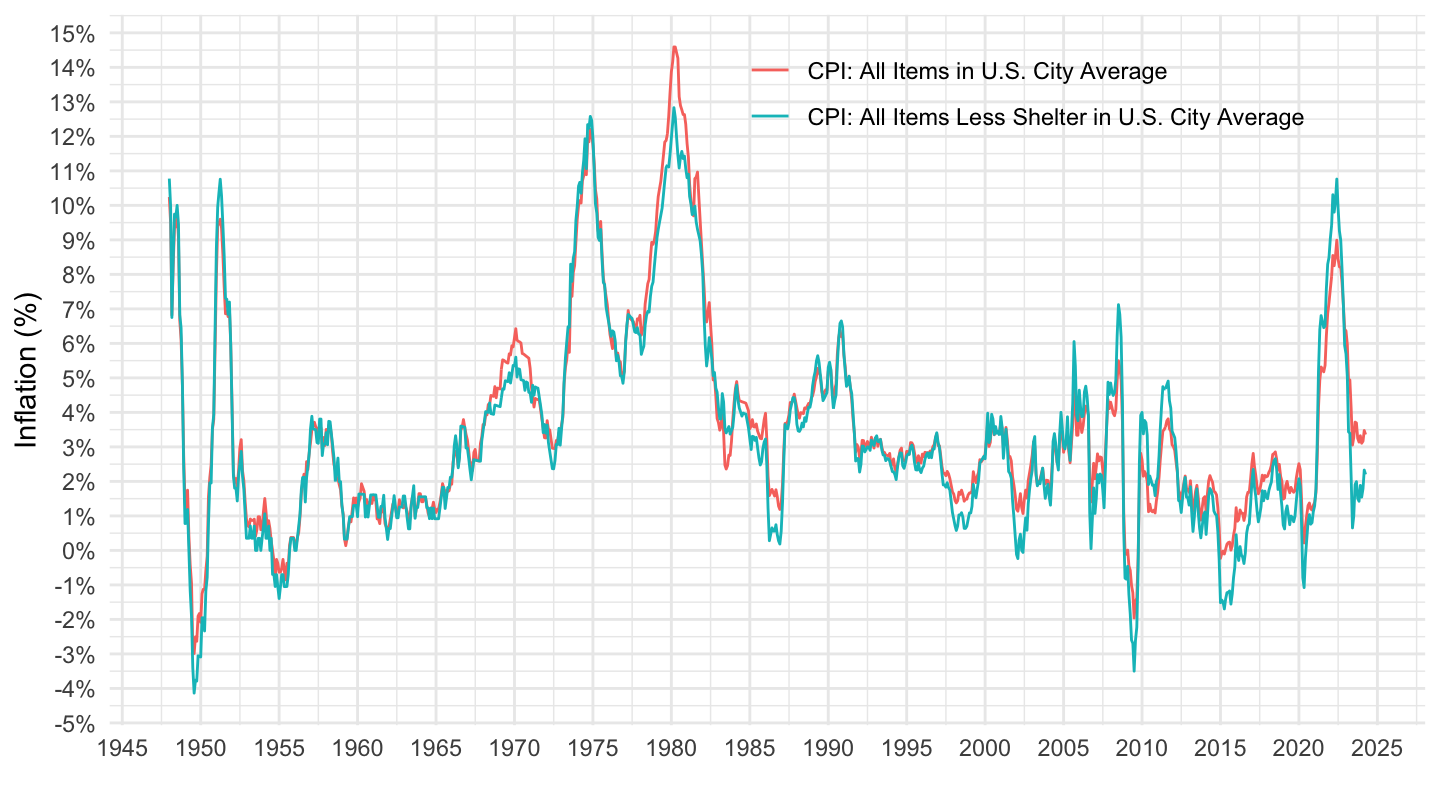
2000-
Code
inflation %>%
  filter(variable %in% c("CPIAUCSL", "CUUR0000SA0L2"),
         date >= as.Date("2000-01-01")) %>%
  select(date, variable, value) %>%
  group_by(variable) %>%
  arrange(date) %>%
  mutate(value = value/lag(value, 12) - 1) %>%
  left_join(variable, by = "variable") %>%
  na.omit %>%
  mutate(Variable = gsub("Consumer Price Index for All Urban Consumers", "CPI", Variable)) %>%
  ggplot(.) + geom_line(aes(x = date, y = value, color = Variable)) + theme_minimal() +
  scale_x_date(breaks = seq(1870, 2100, 2) %>% paste0("-01-01") %>% as.Date,
               labels = date_format("%Y")) +
  scale_y_continuous(breaks = 0.01*seq(-60, 60, 1),
                     labels = scales::percent_format(accuracy = 1)) +
  xlab("") + ylab("Inflation (%)") +
  theme(legend.position = c(0.5, 0.9),
        legend.title = element_blank())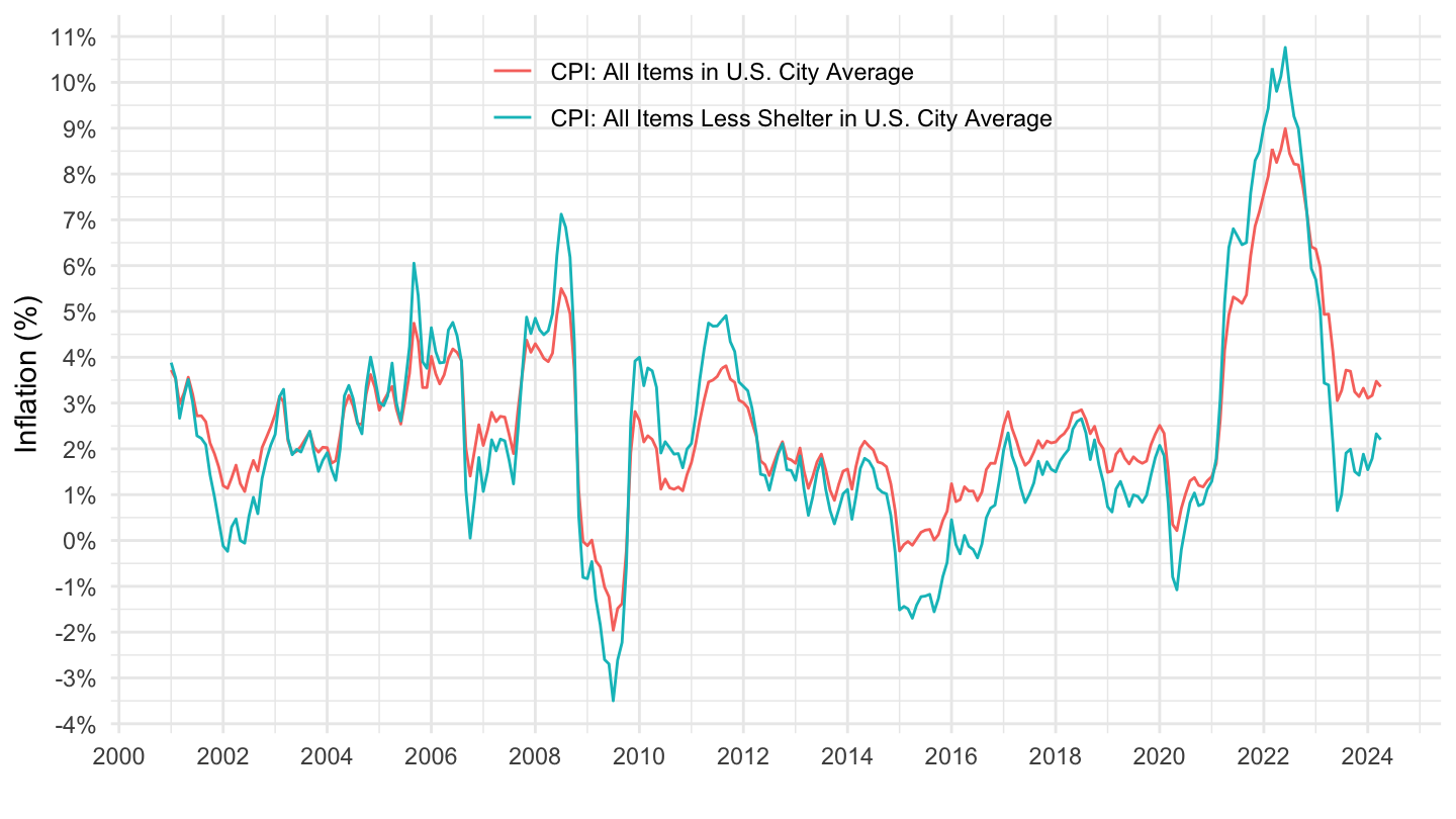
2010-
Code
inflation %>%
  filter(variable %in% c("CPIAUCSL", "CUUR0000SA0L2"),
         date >= as.Date("2010-01-01")) %>%
  select(date, variable, value) %>%
  group_by(variable) %>%
  arrange(date) %>%
  mutate(value = value/lag(value, 12) - 1) %>%
  left_join(variable, by = "variable") %>%
  na.omit %>%
  mutate(Variable = gsub("Consumer Price Index for All Urban Consumers", "CPI", Variable)) %>%
  ggplot(.) + geom_line(aes(x = date, y = value, color = Variable)) + theme_minimal() +
  scale_x_date(breaks = seq(1870, 2100, 1) %>% paste0("-01-01") %>% as.Date,
               labels = date_format("%Y")) +
  scale_y_continuous(breaks = 0.01*seq(-60, 60, 1),
                     labels = scales::percent_format(accuracy = 1)) +
  xlab("") + ylab("Inflation (%)") +
  theme(legend.position = c(0.5, 0.9),
        legend.title = element_blank())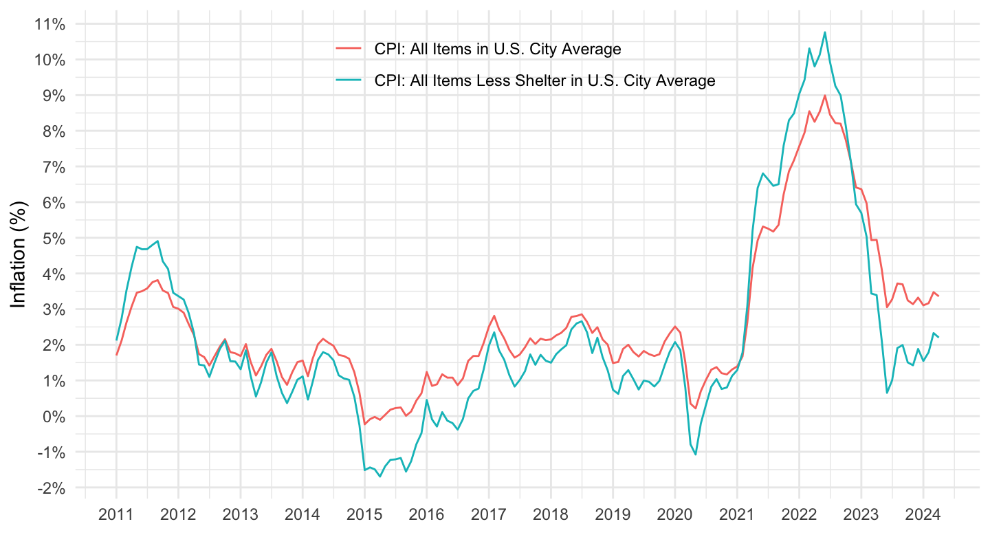
2017-
Code
inflation %>%
  filter(variable %in% c("CPIAUCSL", "CUUR0000SA0L2"),
         date >= as.Date("2017-01-01")) %>%
  select(date, variable, value) %>%
  group_by(variable) %>%
  arrange(date) %>%
  mutate(value = value/lag(value, 12) - 1) %>%
  left_join(variable, by = "variable") %>%
  na.omit %>%
  mutate(Variable = gsub("Consumer Price Index for All Urban Consumers", "CPI", Variable)) %>%
  ggplot(.) + geom_line(aes(x = date, y = value, color = Variable)) + theme_minimal() +
  scale_x_date(breaks = seq(1870, 2100, 1) %>% paste0("-01-01") %>% as.Date,
               labels = date_format("%Y")) +
  scale_y_continuous(breaks = 0.01*seq(-60, 60, 1),
                     labels = scales::percent_format(accuracy = 1)) +
  xlab("") + ylab("Inflation (%)") +
  theme(legend.position = c(0.5, 0.9),
        legend.title = element_blank())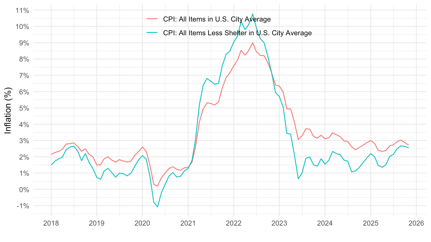
2 years
Code
inflation %>%
  filter(variable %in% c("CPIAUCSL", "CUUR0000SA0L2")) %>%
  select(date, variable, value) %>%
  group_by(variable) %>%
  arrange(date) %>%
  mutate(value = value/lag(value, 12) - 1) %>%
  filter(date >= Sys.Date() - years(3)) %>%
  left_join(variable, by = "variable") %>%
  na.omit %>%
  mutate(Variable = gsub("Consumer Price Index for All Urban Consumers", "CPI", Variable)) %>%
  ggplot(.) + geom_line(aes(x = date, y = value, color = Variable)) + theme_minimal() +
  scale_x_date(breaks = "2 months",
               labels = date_format("%b %Y")) +
  scale_y_continuous(breaks = 0.01*seq(-60, 60, 1),
                     labels = scales::percent_format(accuracy = 1)) +
  xlab("") + ylab("Inflation (%)") +
  theme(legend.position = c(0.5, 0.2),
        legend.title = element_blank(),
        axis.text.x = element_text(angle = 45, vjust = 1, hjust = 1))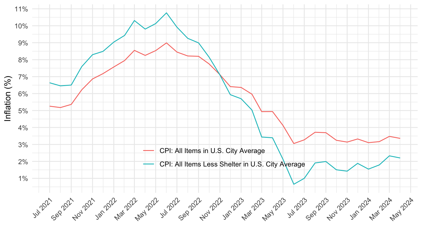
Inflation U.S.
Consumer Inflation Expectations - MICH
All
Code
inflation %>%
  filter(variable %in% c("MICH")) %>%
  left_join(variable, by = "variable") %>%
  ggplot(.) + geom_line(aes(x = date, y = value / 100)) + theme_minimal() +
  scale_x_date(breaks = seq(1870, 2025, 5) %>% paste0("-01-01") %>% as.Date,
               labels = date_format("%Y")) +
  scale_y_continuous(breaks = 0.01*seq(-60, 60, 1),
                     labels = scales::percent_format(accuracy = 1)) +
  xlab("") + ylab("Michigan Consumper Expectations (%)") +
  scale_color_manual(values = c("#2D68C4", "#F2A900", "#000000")) +
  theme(legend.position = c(0.5, 0.9),
        legend.title = element_blank())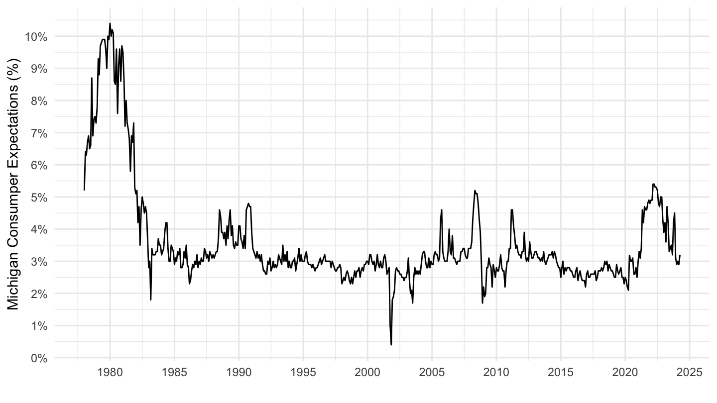
1985-
Code
inflation %>%
  filter(variable %in% c("MICH")) %>%
  left_join(variable, by = "variable") %>%
  filter(date >= as.Date("1985-01-01")) %>%
  ggplot(.) + geom_line(aes(x = date, y = value / 100)) + theme_minimal() +
  scale_x_date(breaks = seq(1870, 2100, 5) %>% paste0("-01-01") %>% as.Date,
               labels = date_format("%Y")) +
  scale_y_continuous(breaks = 0.01*seq(-60, 60, 1),
                     labels = scales::percent_format(accuracy = 1)) +
  xlab("") + ylab("Michigan Consumper Expectations (%)") +
  scale_color_manual(values = c("#2D68C4", "#F2A900", "#000000")) +
  theme(legend.position = c(0.5, 0.9),
        legend.title = element_blank())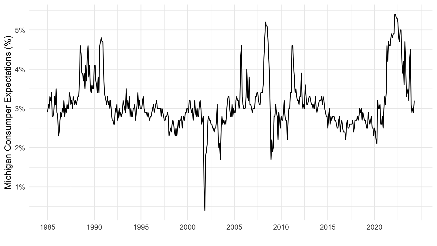
1995-
Code
inflation %>%
  filter(variable %in% c("MICH")) %>%
  left_join(variable, by = "variable") %>%
  filter(date >= "1995-01-01") %>%
  ggplot(.) + geom_line(aes(x = date, y = value / 100)) + theme_minimal() +
  scale_x_date(breaks = seq(1870, 2100, 5) %>% paste0("-01-01") %>% as.Date,
               labels = date_format("%Y")) +
  scale_y_continuous(breaks = 0.01*seq(-60, 60, 1),
                     labels = scales::percent_format(accuracy = 1)) +
  xlab("") + ylab("Michigan Consumper Expectations (%)") +
  scale_color_manual(values = c("#2D68C4", "#F2A900", "#000000")) +
  theme(legend.position = c(0.5, 0.9),
        legend.title = element_blank())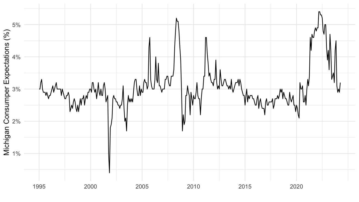
CPI, PCE, A255RD3Q086SBEA
1945-1970
Same Scale
Code
inflation %>%
  filter(variable %in% c("CPIAUCSL", "A255RD3Q086SBEA"),
         month(date) == 1,
         date >= as.Date("1945-01-01"),
         date <= as.Date("1970-01-01")) %>%
  select(date, variable, value) %>%
  spread(variable, value) %>%
  mutate(CPIAUCSL = 100*(log(CPIAUCSL) - lag(log(CPIAUCSL))),
         A255RD3Q086SBEA = 100*(log(A255RD3Q086SBEA) - lag(log(A255RD3Q086SBEA)))) %>%
  gather(variable, value, -date) %>%
  left_join(variable, by = "variable") %>%
  ggplot(.) + geom_line(aes(x = date, y = value / 100, color = Variable)) + theme_minimal() +
  scale_x_date(breaks = seq(1870, 2100, 5) %>% paste0("-01-01") %>% as.Date,
               labels = date_format("%Y")) +
  scale_y_continuous(breaks = 0.01*seq(-60, 60, 5),
                     labels = scales::percent_format(accuracy = 1)) +
  xlab("") + ylab("Inflation Rates (%)") +
  scale_color_manual(values = c("#2D68C4", "#F2A900", "#000000")) +
  theme(legend.position = c(0.5, 0.9),
        legend.title = element_blank())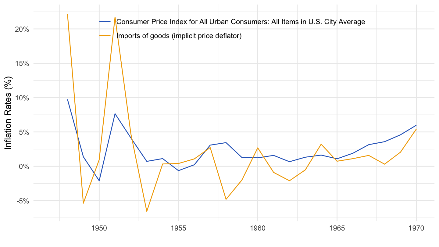
Different Scale
Code
inflation %>%
  filter(variable %in% c("CPIAUCSL", "A255RD3Q086SBEA"),
         month(date) == 1,
         date >= as.Date("1945-01-01"),
         date <= as.Date("1970-01-01")) %>%
  select(date, variable, value) %>%
  spread(variable, value) %>%
  mutate(CPIAUCSL = 100*(log(CPIAUCSL) - lag(log(CPIAUCSL))),
         A255RD3Q086SBEA = 20*(log(A255RD3Q086SBEA) - lag(log(A255RD3Q086SBEA)))) %>%
  gather(variable, value, -date) %>%
  left_join(variable, by = "variable") %>%
  ggplot(.) + geom_line(aes(x = date, y = value / 100, color = Variable)) + theme_minimal() +
  scale_x_date(breaks = seq(1870, 2100, 5) %>% paste0("-01-01") %>% as.Date,
               labels = date_format("%Y")) +
  scale_y_continuous(breaks = 0.01*seq(-60, 60, 1),
                     labels = scales::percent_format(accuracy = 1),
                     limits = c(-0.035, 0.16)) +
  xlab("") + ylab("Inflation Rates (%) - CPI, Imports of goods/5") +
  scale_color_manual(values = c("#2D68C4", "#F2A900")) +
  theme(legend.position = c(0.5, 0.9),
        legend.title = element_blank())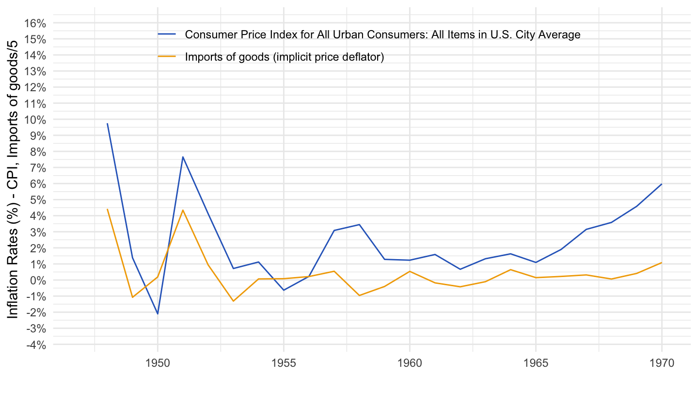
1945-
Code
inflation %>%
  filter(variable %in% c("DPCCRV1Q225SBEA", "CPIAUCSL", "A255RD3Q086SBEA"),
         month(date) == 1,
         date >= as.Date("1945-01-01")) %>%
  select(date, variable, value) %>%
  spread(variable, value) %>%
  mutate(CPIAUCSL = 100*(log(CPIAUCSL) - lag(log(CPIAUCSL))),
         A255RD3Q086SBEA = 100*(log(A255RD3Q086SBEA) - lag(log(A255RD3Q086SBEA)))) %>%
  gather(variable, value, -date) %>%
  left_join(variable, by = "variable") %>%
  ggplot(.) + geom_line(aes(x = date, y = value / 100, color = Variable)) + theme_minimal() +
  scale_x_date(breaks = seq(1870, 2100, 5) %>% paste0("-01-01") %>% as.Date,
               labels = date_format("%Y")) +
  scale_y_continuous(breaks = 0.01*seq(-60, 60, 5),
                     labels = scales::percent_format(accuracy = 1)) +
  xlab("") + ylab("Inflation Rates (%)") +
  scale_color_manual(values = c("#2D68C4", "#F2A900", "#000000")) +
  theme(legend.position = c(0.5, 0.9),
        legend.title = element_blank())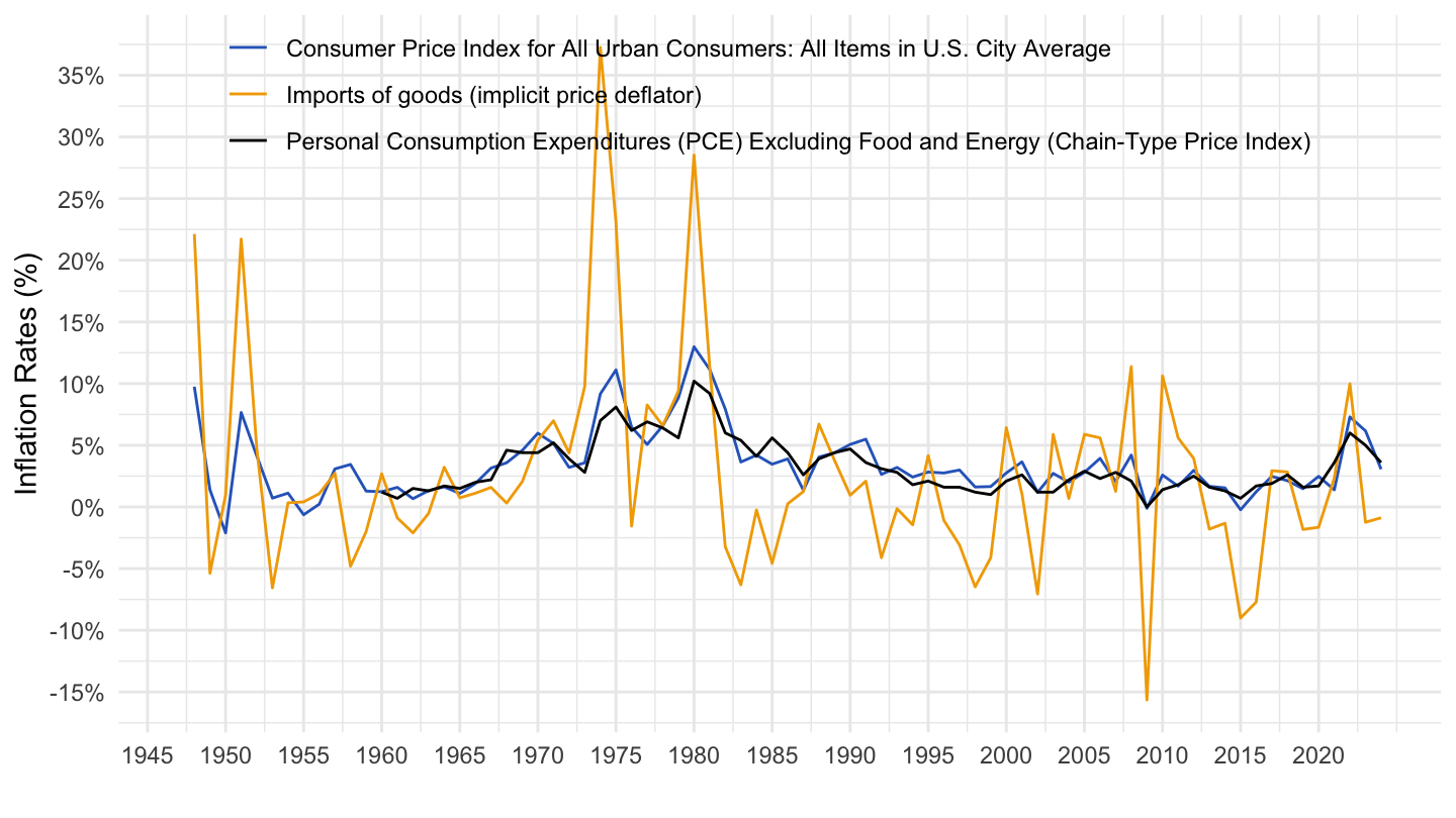
1960-
Same Scale
Code
inflation %>%
  filter(variable %in% c("CPIAUCSL", "A255RD3Q086SBEA"),
         month(date) == 1,
         date >= as.Date("1960-01-01")) %>%
  select(date, variable, value) %>%
  spread(variable, value) %>%
  mutate(CPIAUCSL = 100*(log(CPIAUCSL) - lag(log(CPIAUCSL))),
         A255RD3Q086SBEA = 100*(log(A255RD3Q086SBEA) - lag(log(A255RD3Q086SBEA)))) %>%
  gather(variable, value, -date) %>%
  left_join(variable, by = "variable") %>%
  ggplot(.) + geom_line(aes(x = date, y = value / 100, color = Variable)) + theme_minimal() +
  scale_x_date(breaks = seq(1870, 2100, 5) %>% paste0("-01-01") %>% as.Date,
               labels = date_format("%Y")) +
  scale_y_continuous(breaks = 0.01*seq(-60, 60, 5),
                     labels = scales::percent_format(accuracy = 1)) +
  xlab("") + ylab("Inflation Rates (%)") +
  scale_color_manual(values = c("#2D68C4", "#F2A900")) +
  theme(legend.position = c(0.5, 0.9),
        legend.title = element_blank())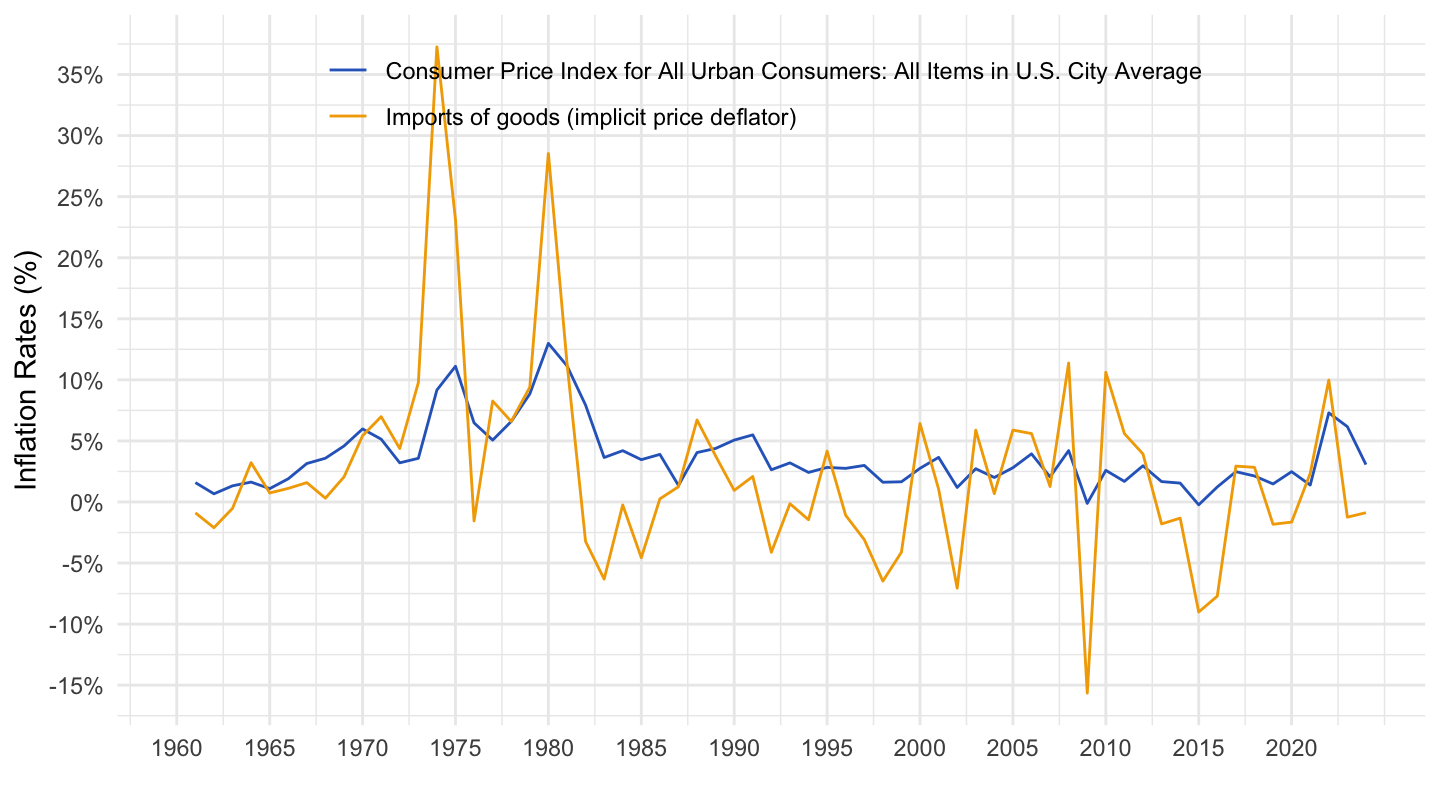
Different Scale
Code
inflation %>%
  filter(variable %in% c("CPIAUCSL", "A255RD3Q086SBEA"),
         month(date) == 1,
         date >= as.Date("1960-01-01")) %>%
  select(date, variable, value) %>%
  spread(variable, value) %>%
  mutate(CPIAUCSL = 100*(log(CPIAUCSL) - lag(log(CPIAUCSL))),
         A255RD3Q086SBEA = 20*(log(A255RD3Q086SBEA) - lag(log(A255RD3Q086SBEA)))) %>%
  gather(variable, value, -date) %>%
  left_join(variable, by = "variable") %>%
  ggplot(.) + geom_line(aes(x = date, y = value / 100, color = Variable)) + theme_minimal() +
  scale_x_date(breaks = seq(1870, 2100, 5) %>% paste0("-01-01") %>% as.Date,
               labels = date_format("%Y")) +
  scale_y_continuous(breaks = 0.01*seq(-60, 60, 1),
                     labels = scales::percent_format(accuracy = 1),
                     limits = c(-0.035, 0.16)) +
  xlab("") + ylab("Inflation Rates (%) - CPI, Imports of goods/5") +
  scale_color_manual(values = c("#2D68C4", "#F2A900")) +
  theme(legend.position = c(0.5, 0.9),
        legend.title = element_blank())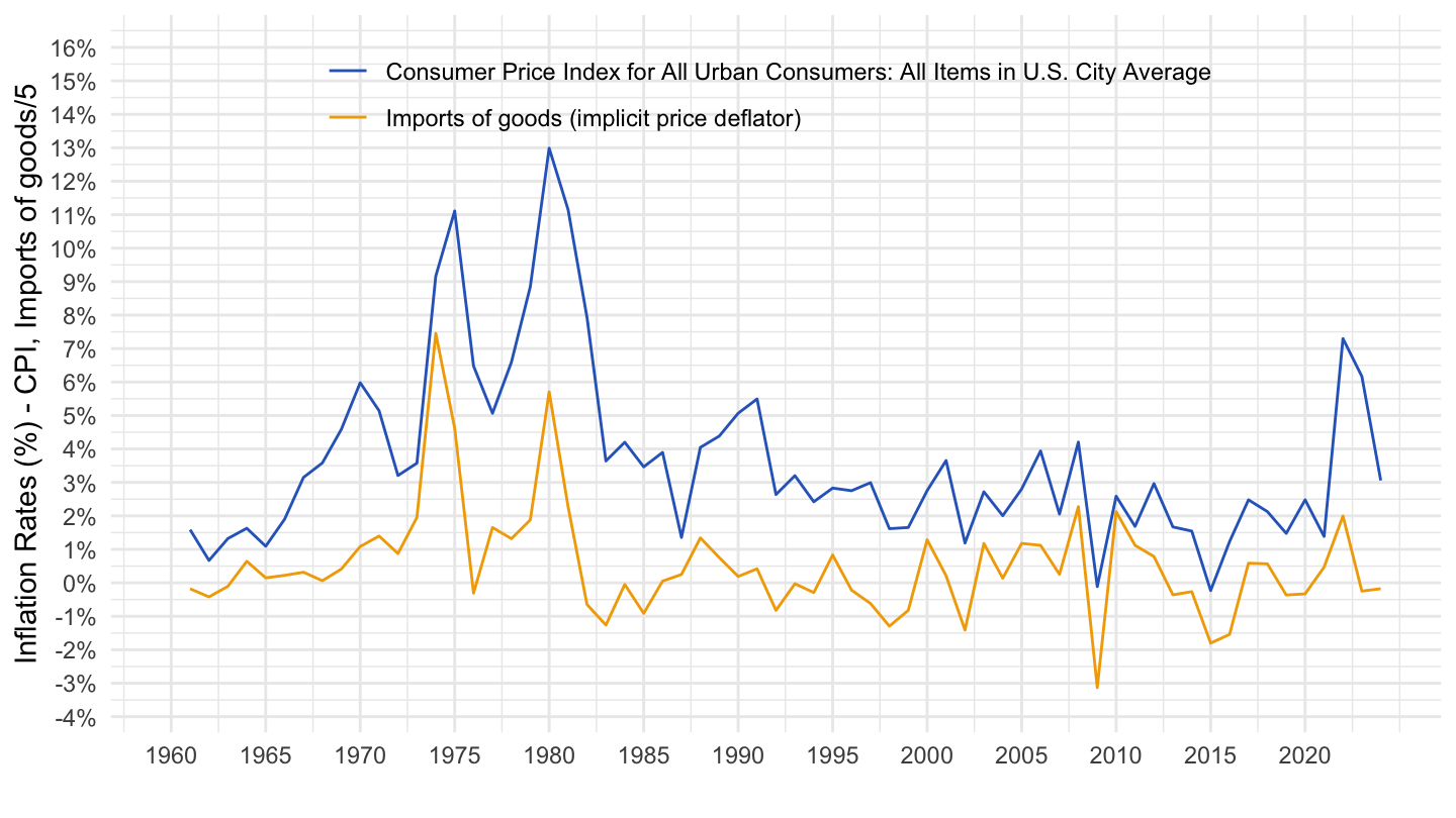
1995-
Code
inflation %>%
  filter(variable %in% c("CPIAUCSL", "A255RD3Q086SBEA"),
         month(date) == 1,
         date >= as.Date("1995-01-01")) %>%
  select(date, variable, value) %>%
  spread(variable, value) %>%
  mutate(CPIAUCSL = 100*(log(CPIAUCSL) - lag(log(CPIAUCSL))),
         A255RD3Q086SBEA = 20*(log(A255RD3Q086SBEA) - lag(log(A255RD3Q086SBEA)))) %>%
  gather(variable, value, -date) %>%
  left_join(variable, by = "variable") %>%
  ggplot(.) + geom_line(aes(x = date, y = value / 100, color = Variable)) + theme_minimal() +
  scale_x_date(breaks = seq(1870, 2100, 5) %>% paste0("-01-01") %>% as.Date,
               labels = date_format("%Y")) +
  scale_y_continuous(breaks = 0.01*seq(-60, 60, 1),
                     labels = scales::percent_format(accuracy = 1),
                     limits = c(-0.035, 0.06)) +
  xlab("") + ylab("Inflation Rates (%) - CPI, Imports of goods/5") +
  scale_color_manual(values = c("#2D68C4", "#F2A900")) +
  theme(legend.position = c(0.5, 0.9),
        legend.title = element_blank())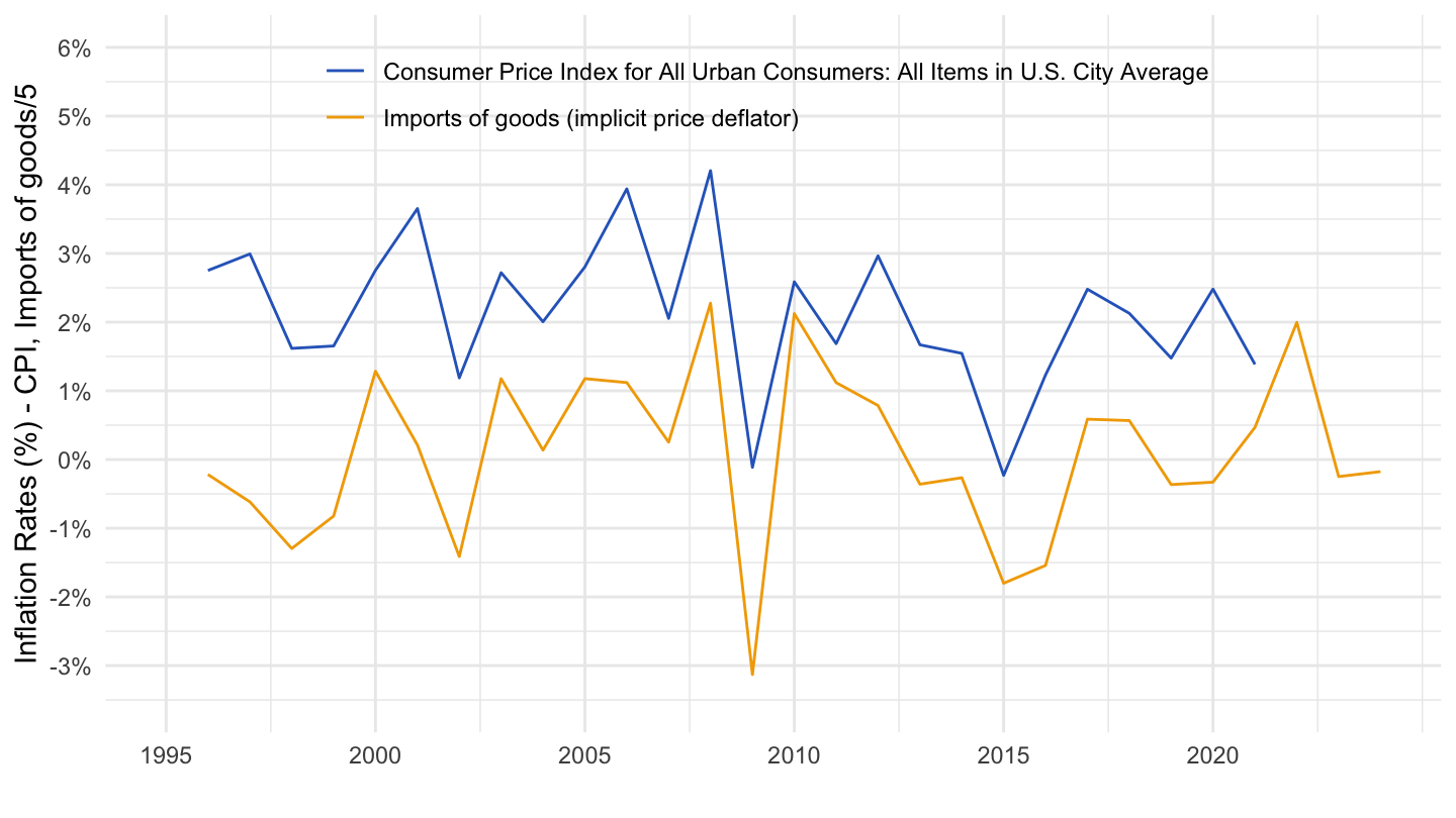
1990-2005
Code
inflation %>%
  filter(variable %in% c("CPIAUCSL", "A255RD3Q086SBEA"),
         month(date) == 1,
         date >= as.Date("1990-01-01"),
         date <= as.Date("2005-01-01")) %>%
  select(date, variable, value) %>%
  spread(variable, value) %>%
  mutate(CPIAUCSL = 100*(log(CPIAUCSL) - lag(log(CPIAUCSL))),
         A255RD3Q086SBEA = 20*(log(A255RD3Q086SBEA) - lag(log(A255RD3Q086SBEA)))) %>%
  gather(variable, value, -date) %>%
  left_join(variable, by = "variable") %>%
  ggplot(.) + geom_line(aes(x = date, y = value / 100, color = Variable)) + theme_minimal() +
  scale_x_date(breaks = seq(1870, 2100, 2) %>% paste0("-01-01") %>% as.Date,
               labels = date_format("%Y")) +
  scale_y_continuous(breaks = 0.01*seq(-60, 60, 1),
                     labels = scales::percent_format(accuracy = 1),
                     limits = c(-0.035, 0.06)) +
  xlab("") + ylab("Inflation Rates (%) - CPI, Imports of goods/5") +
  scale_color_manual(values = c("#2D68C4", "#F2A900")) +
  theme(legend.position = c(0.5, 0.9),
        legend.title = element_blank())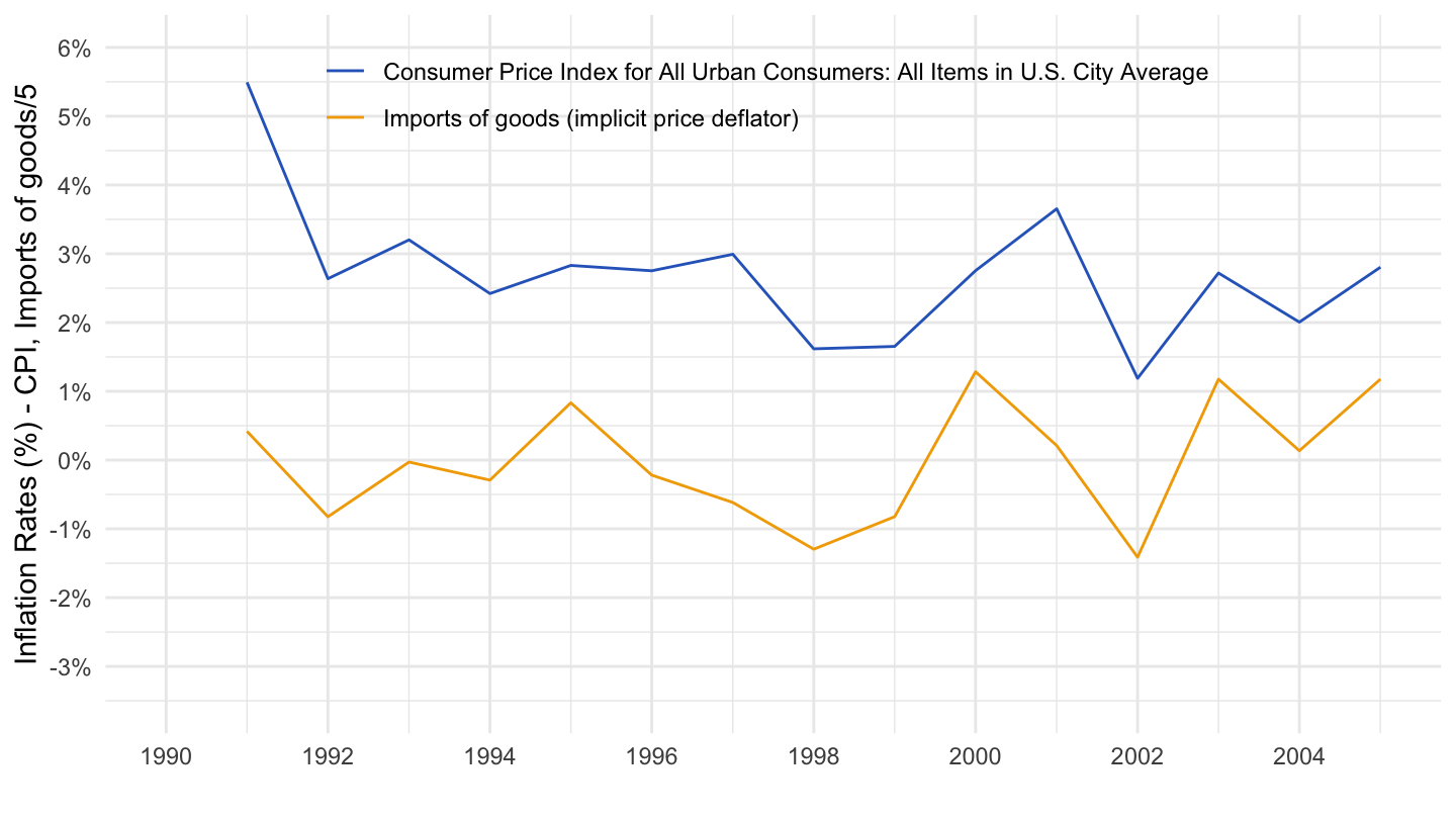
1960-1980
Same scale
Code
inflation %>%
  filter(variable %in% c("CPIAUCSL", "A255RD3Q086SBEA"),
         month(date) == 1,
         date >= as.Date("1960-01-01"),
         date <= as.Date("1980-01-01")) %>%
  select(date, variable, value) %>%
  spread(variable, value) %>%
  mutate(CPIAUCSL = 100*(log(CPIAUCSL) - lag(log(CPIAUCSL))),
         A255RD3Q086SBEA = 100*(log(A255RD3Q086SBEA) - lag(log(A255RD3Q086SBEA)))) %>%
  gather(variable, value, -date) %>%
  left_join(variable, by = "variable") %>%
  ggplot(.) + geom_line(aes(x = date, y = value / 100, color = Variable)) + theme_minimal() +
  scale_x_date(breaks = seq(1870, 2100, 2) %>% paste0("-01-01") %>% as.Date,
               labels = date_format("%Y")) +
  scale_y_continuous(breaks = 0.01*seq(-60, 60, 2),
                     labels = scales::percent_format(accuracy = 1)) +
  xlab("") + ylab("Inflation Rates (%) - CPI, Imports of goods") +
  scale_color_manual(values = c("#2D68C4", "#F2A900")) +
  theme(legend.position = c(0.5, 0.9),
        legend.title = element_blank())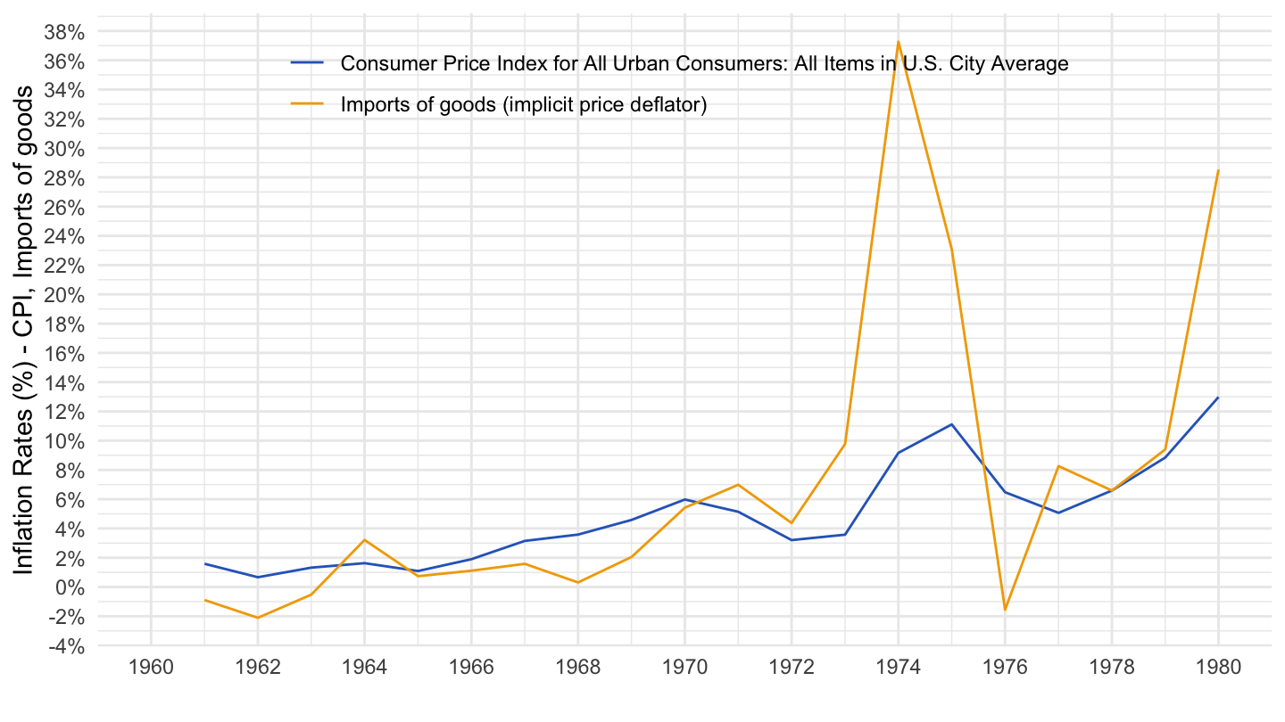
Scale divided by 5
Code
inflation %>%
  filter(variable %in% c("CPIAUCSL", "A255RD3Q086SBEA"),
         month(date) == 1,
         date >= as.Date("1960-01-01"),
         date <= as.Date("1980-01-01")) %>%
  select(date, variable, value) %>%
  spread(variable, value) %>%
  mutate(CPIAUCSL = 100*(log(CPIAUCSL) - lag(log(CPIAUCSL))),
         A255RD3Q086SBEA = 20*(log(A255RD3Q086SBEA) - lag(log(A255RD3Q086SBEA)))) %>%
  gather(variable, value, -date) %>%
  left_join(variable, by = "variable") %>%
  ggplot(.) + geom_line(aes(x = date, y = value / 100, color = Variable)) + theme_minimal() +
  scale_x_date(breaks = seq(1870, 2100, 2) %>% paste0("-01-01") %>% as.Date,
               labels = date_format("%Y")) +
  scale_y_continuous(breaks = 0.01*seq(-60, 60, 1),
                     labels = scales::percent_format(accuracy = 1)) +
  xlab("") + ylab("Inflation Rates (%) - CPI, Imports of goods/5") +
  scale_color_manual(values = c("#2D68C4", "#F2A900")) +
  theme(legend.position = c(0.5, 0.9),
        legend.title = element_blank())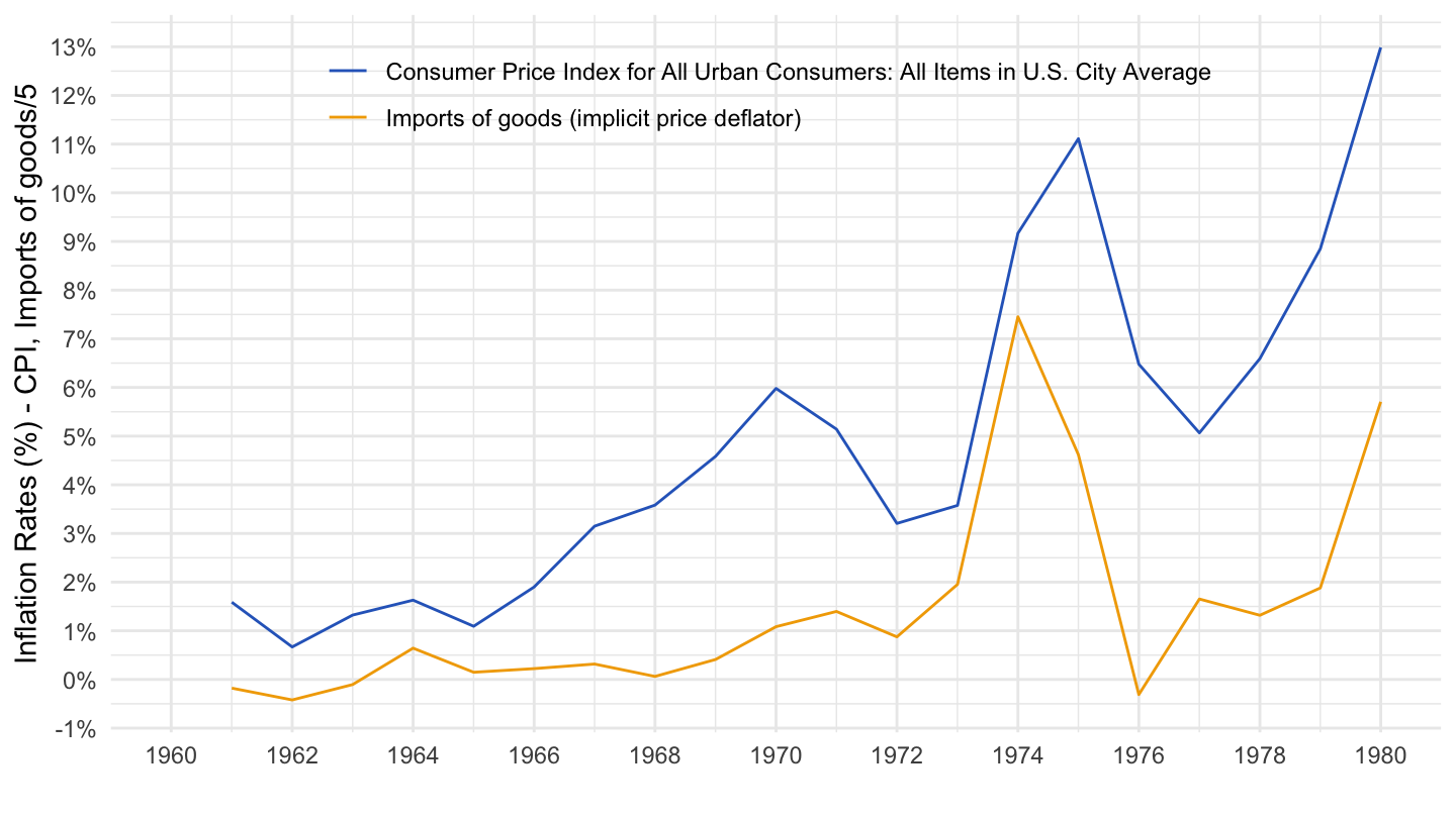
Inflation
Code
inflation %>%
  filter(variable %in% c("DPCCRV1Q225SBEA")) %>%
  left_join(variable, by = "variable") %>%
  ggplot(.) + geom_line(aes(x = date, y = value / 100, color = Variable)) + theme_minimal() +
  scale_x_date(breaks = seq(1870, 2100, 5) %>% paste0("-01-01") %>% as.Date,
               labels = date_format("%Y")) +
  scale_y_continuous(breaks = 0.01*seq(-10, 15, 1),
                     labels = scales::percent_format(accuracy = 1)) +
  xlab("") + ylab("Breakeven Inflation Rates (%)") +

  theme(legend.position = c(0.7, 0.2),
        legend.title = element_blank())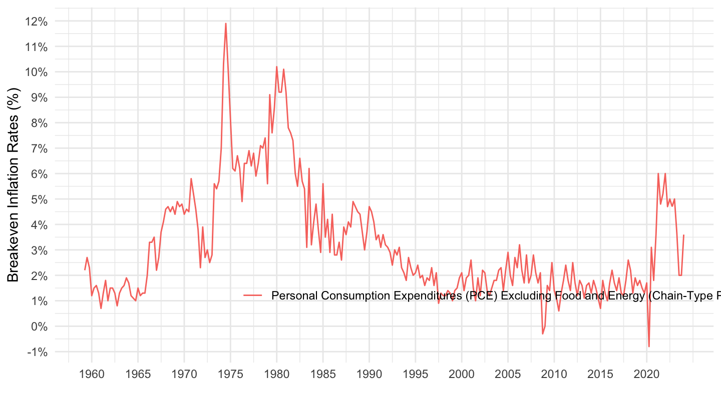
AFGAP Graph
All
- Association Française des Gestionnaires Actif-Passif - AFGAP. pdf
Code
inflation %>%
  filter(variable %in% c("DPCCRV1Q225SBEA", "CPIAUCSL"),
         month(date) == 1,
         date >= as.Date("1960-01-01")) %>%
  select(date, variable, value) %>%
  spread(variable, value) %>%
  mutate(CPIAUCSL = 100*(log(CPIAUCSL) - lag(log(CPIAUCSL)))) %>%
  gather(variable, value, -date) %>%
  left_join(variable, by = "variable") %>%
  ggplot(.) + geom_line(aes(x = date, y = value / 100, color = Variable)) + theme_minimal() +
  scale_x_date(breaks = seq(1870, 2100, 5) %>% paste0("-01-01") %>% as.Date,
               labels = date_format("%Y")) +
  scale_y_continuous(breaks = 0.01*seq(-10, 18, 1),
                     labels = scales::percent_format(accuracy = 1),
                     limits = c(-0.01, 0.18)) +
  xlab("") + ylab("Inflation Rates (%)") +
  scale_color_manual(values = c("#2D68C4", "#F2A900")) +
  theme(legend.position = c(0.5, 0.9),
        legend.title = element_blank())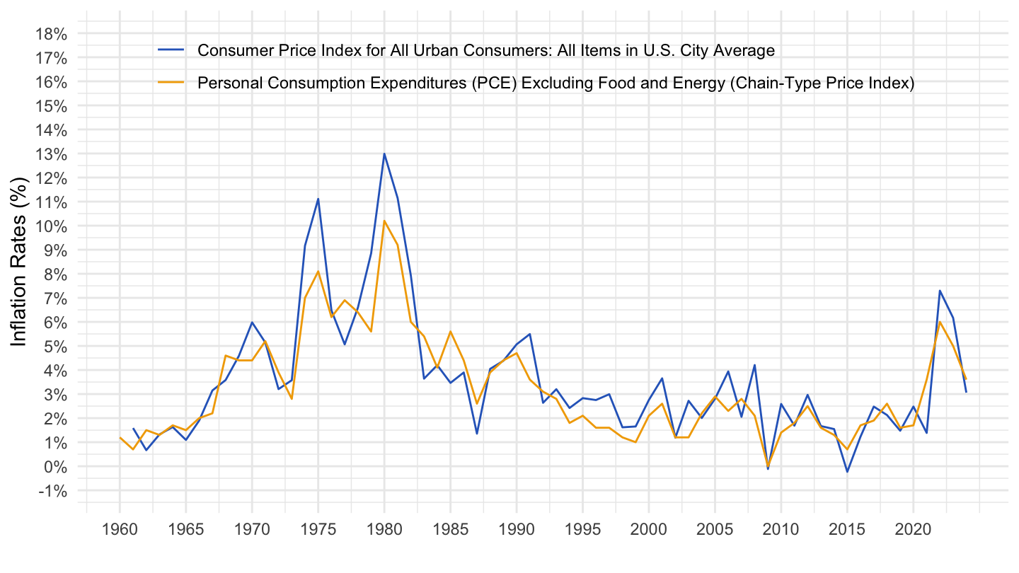
US-Presidents
Code
inflation %>%
  filter(variable %in% c("DPCCRV1Q225SBEA", "CPIAUCSL"),
         month(date) == 1,
         date >= as.Date("1960-01-01")) %>%
  select(date, variable, value) %>%
  spread(variable, value) %>%
  mutate(CPIAUCSL = 100*(log(CPIAUCSL) - lag(log(CPIAUCSL)))) %>%
  gather(variable, value, -date) %>%
  left_join(variable, by = "variable") %>%
  ggplot(.) + geom_line(aes(x = date, y = value / 100, color = Variable)) + theme_minimal() +
  scale_x_date(breaks = seq(1870, 2100, 5) %>% paste0("-01-01") %>% as.Date,
               labels = date_format("%Y")) +
  scale_y_continuous(breaks = 0.01*seq(-10, 18, 1),
                     labels = scales::percent_format(accuracy = 1),
                     limits = c(-0.02, 0.16)) +
  xlab("") + ylab("Inflation Rates (%)") +
  scale_color_manual(values = c("#2D68C4", "#F2A900")) +
  geom_vline(aes(xintercept = as.numeric(start)),
             data = US_presidents %>%
               filter(start >= as.Date("1960-01-01")) %>%
               select(-party),
             colour = "grey50", alpha = 0.5) +
  geom_rect(aes(xmin = start, xmax = end, fill = party),
         ymin = -Inf, ymax = Inf, alpha = 0.1,
         data = US_presidents %>%
               filter(start >= as.Date("1960-01-01"))) +
  geom_text(aes(x = start, y = new, label = name),
            data = US_presidents %>%
              filter(start >= as.Date("1960-01-01")) %>%
              mutate(new = -0.01 + 0.005 * (1:n() %% 2)) %>%
              select(-party),
            size = 2.5, vjust = 0, hjust = 0, nudge_x = 50) +
  scale_fill_manual(values = c("white", "grey")) +
  theme(legend.position = c(0.5, 1),
        legend.title = element_blank())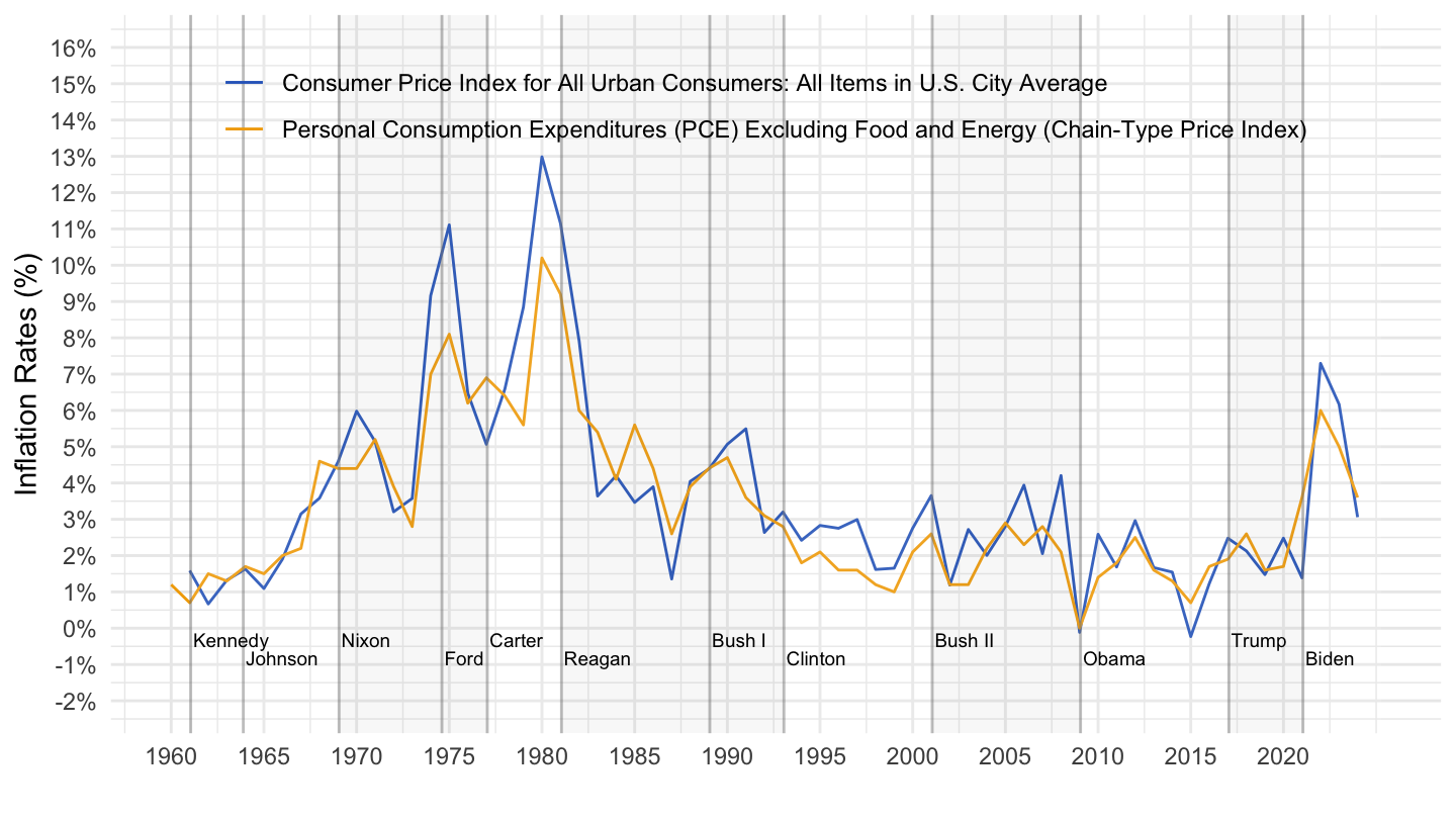
Regressions
All
Code
fit1 <- inflation %>%
  filter(variable %in% c("CPIAUCSL", "A255RD3Q086SBEA"),
         month(date) == 1) %>%
  select(date, variable, value) %>%
  spread(variable, value) %>%
  mutate(CPIAUCSL = 100*(log(CPIAUCSL) - lag(log(CPIAUCSL))),
         A255RD3Q086SBEA = 100*(log(A255RD3Q086SBEA) - lag(log(A255RD3Q086SBEA)))) %>%
  lm(CPIAUCSL ~ A255RD3Q086SBEA, data = .)

summary(fit1)
#
# Call:
# lm(formula = CPIAUCSL ~ A255RD3Q086SBEA, data = .)
#
# Residuals:
# Min 1Q Median 3Q Max
# -5.1366 -1.2571 -0.1283 0.9537 5.9348
#
# Coefficients:
# Estimate Std. Error t value Pr(>|t|)
# (Intercept) 2.79569 0.23173 12.064 < 2e-16 ***
# A255RD3Q086SBEA 0.24661 0.02744 8.989 1.26e-13 ***
# ---
# Signif. codes: 0 '***' 0.001 '**' 0.01 '*' 0.05 '.' 0.1 ' ' 1
#
# Residual standard error: 1.957 on 77 degrees of freedom
# (1 observation effacée parce que manquante)
# Multiple R-squared: 0.512, Adjusted R-squared: 0.5057
# F-statistic: 80.79 on 1 and 77 DF, p-value: 1.262e-131945-1970
Code
fit2 <- inflation %>%
  filter(variable %in% c("CPIAUCSL", "A255RD3Q086SBEA"),
         month(date) == 1,
         date >= as.Date("1945-01-01"),
         date <= as.Date("1970-01-01")) %>%
  select(date, variable, value) %>%
  spread(variable, value) %>%
  mutate(CPIAUCSL = 100*(log(CPIAUCSL) - lag(log(CPIAUCSL))),
         A255RD3Q086SBEA = 100*(log(A255RD3Q086SBEA) - lag(log(A255RD3Q086SBEA)))) %>%
  lm(CPIAUCSL ~ A255RD3Q086SBEA, data = .)

summary(fit2)
#
# Call:
# lm(formula = CPIAUCSL ~ A255RD3Q086SBEA, data = .)
#
# Residuals:
# Min 1Q Median 3Q Max
# -4.2259 -0.8899 0.0160 1.0177 3.0392
#
# Coefficients:
# Estimate Std. Error t value Pr(>|t|)
# (Intercept) 1.83629 0.37729 4.867 8.21e-05 ***
# A255RD3Q086SBEA 0.29736 0.05328 5.582 1.54e-05 ***
# ---
# Signif. codes: 0 '***' 0.001 '**' 0.01 '*' 0.05 '.' 0.1 ' ' 1
#
# Residual standard error: 1.726 on 21 degrees of freedom
# (1 observation effacée parce que manquante)
# Multiple R-squared: 0.5973, Adjusted R-squared: 0.5782
# F-statistic: 31.15 on 1 and 21 DF, p-value: 1.54e-051970-2020
Code
fit3 <- inflation %>%
  filter(variable %in% c("CPIAUCSL", "A255RD3Q086SBEA"),
         month(date) == 1,
         date >= as.Date("1970-01-01")) %>%
  select(date, variable, value) %>%
  spread(variable, value) %>%
  mutate(CPIAUCSL = 100*(log(CPIAUCSL) - lag(log(CPIAUCSL))),
         A255RD3Q086SBEA = 100*(log(A255RD3Q086SBEA) - lag(log(A255RD3Q086SBEA)))) %>%
  lm(CPIAUCSL ~ A255RD3Q086SBEA, data = .)

summary(fit3)
#
# Call:
# lm(formula = CPIAUCSL ~ A255RD3Q086SBEA, data = .)
#
# Residuals:
# Min 1Q Median 3Q Max
# -3.0472 -1.3457 -0.3164 0.7497 5.4838
#
# Coefficients:
# Estimate Std. Error t value Pr(>|t|)
# (Intercept) 3.19278 0.27458 11.628 2.52e-16 ***
# A255RD3Q086SBEA 0.22993 0.03069 7.491 6.56e-10 ***
# ---
# Signif. codes: 0 '***' 0.001 '**' 0.01 '*' 0.05 '.' 0.1 ' ' 1
#
# Residual standard error: 1.948 on 54 degrees of freedom
# (1 observation effacée parce que manquante)
# Multiple R-squared: 0.5096, Adjusted R-squared: 0.5006
# F-statistic: 56.12 on 1 and 54 DF, p-value: 6.56e-10Breakeven inflation rates
2017-2020
Code
inflation %>%
  filter(variable %in% c("T7YIEM", "T5YIE", "T20YIEM", "T10YIE", "T30YIEM"),
         date >= as.Date("2009-01-01")) %>%
  left_join(variable, by = "variable") %>%
  mutate(Variable = gsub("7-year", " 7-year", Variable),
         Variable = gsub("5-Year", " 5-year", Variable)) %>%
  ggplot(.) + geom_line(aes(x = date, y = value / 100, color = Variable)) + theme_minimal() +
  scale_x_date(breaks = seq(1870, 2025, 2) %>% paste0("-01-01") %>% as.Date,
               labels = date_format("%Y")) +
  scale_y_continuous(breaks = 0.01*seq(-10, 15, 0.5),
                     labels = scales::percent_format(accuracy = .1)) +
  xlab("") + ylab("Breakeven Inflation Rates (%)") +

  theme(legend.position = c(0.7, 0.2),
        legend.title = element_blank())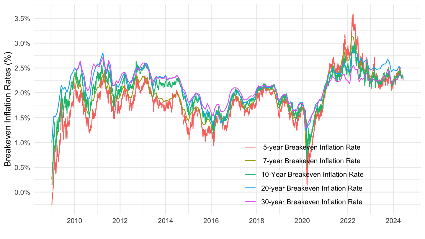
2019-2020
Code
inflation %>%
  filter(variable %in% c("T7YIEM", "T5YIE", "T20YIEM", "T10YIE", "T30YIEM"),
         date >= as.Date("2019-01-01")) %>%
  left_join(variable, by = "variable") %>%
  mutate(Variable = gsub("7-year", " 7-year", Variable),
         Variable = gsub("5-Year", " 5-year", Variable)) %>%
  ggplot(.) + geom_line(aes(x = date, y = value / 100, color = Variable)) + theme_minimal() +
  scale_x_date(breaks = "6 months",
               labels = date_format("%b %y")) +
  scale_y_continuous(breaks = 0.01*seq(-10, 15, 0.5),
                     labels = scales::percent_format(accuracy = .1)) +
  xlab("") + ylab("Breakeven Inflation Rates (%)") +

  theme(legend.position = c(0.7, 0.2),
        legend.title = element_blank())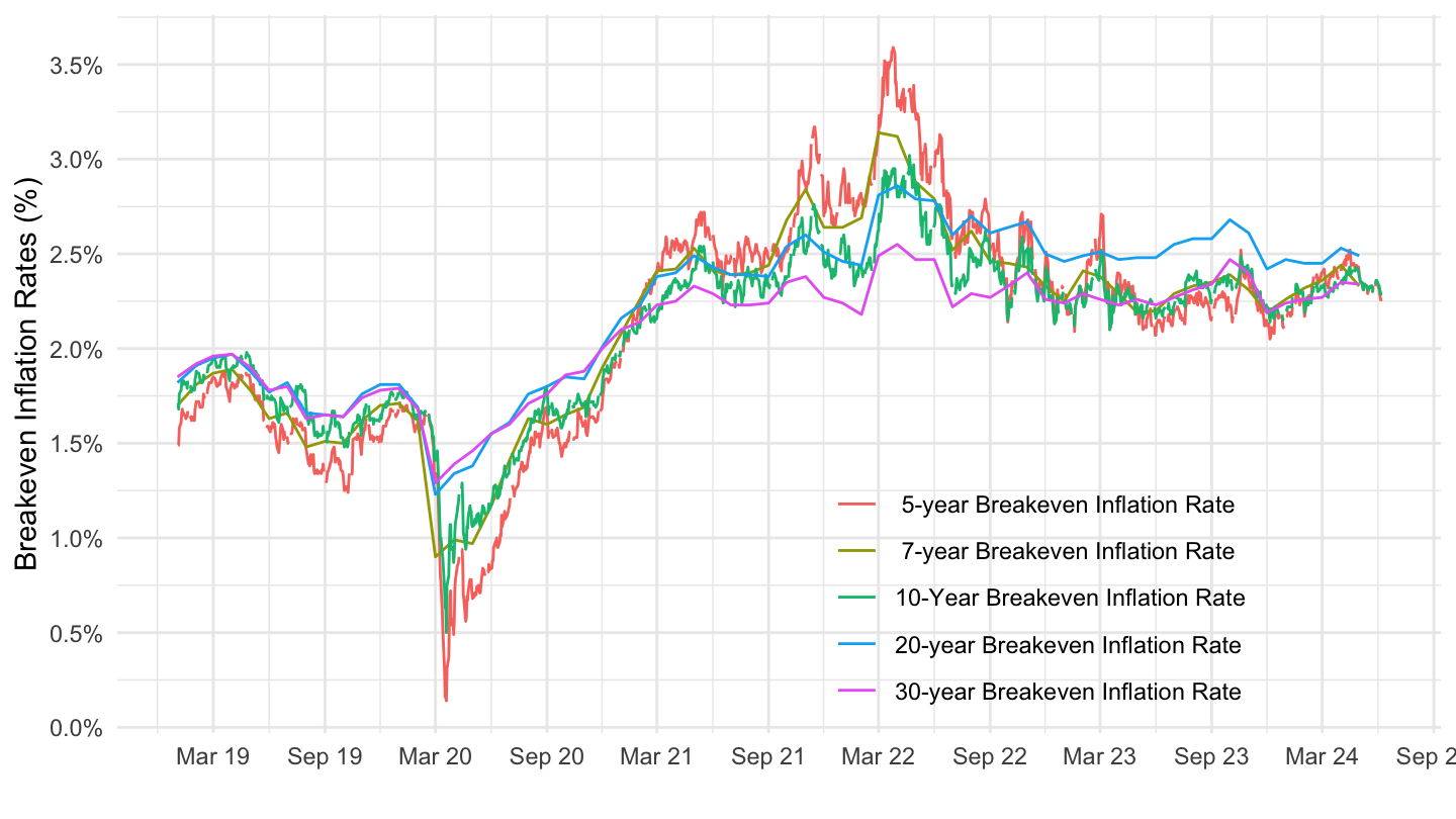
Inflation Expectations
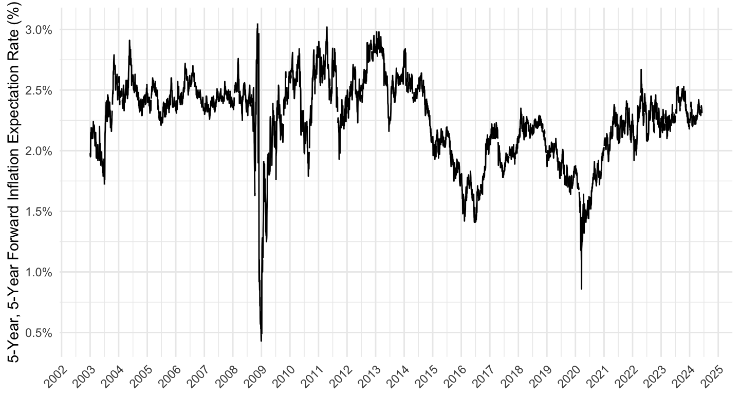
T5YIFR - 5-Year, 5-Year Forward Inflation Expectation Rate
This series is a measure of expected inflation (on average) over the five-year period that begins five years from today.
This series is constructed as: (((((1+((BC_10YEAR-TC_10YEAR)/100))10)/((1+((BC_5YEAR-TC_5YEAR)/100))5))^0.2)-1)*100
where BC10_YEAR, TC_10YEAR, BC_5YEAR, and TC_5YEAR are the 10 year and 5 year nominal and inflation adjusted Treasury securities.
Code
inflation %>%
  filter(variable %in% c("T5YIFR")) %>%
  left_join(variable, by = "variable") %>%
  ggplot(.) + geom_line(aes(x = date, y = value / 100)) + theme_minimal() +
  scale_x_date(breaks = seq(1920, 2100, 1) %>% paste0("-01-01") %>% as.Date,
               labels = date_format("%Y")) +
  scale_y_continuous(breaks = 0.01*seq(-10, 15, 0.5),
                     labels = scales::percent_format(accuracy = .1)) +
  xlab("") + ylab("5-Year, 5-Year Forward Inflation Expectation Rate (%)") +

  theme(legend.position = c(0.7, 0.2),
        legend.title = element_blank(),
        axis.text.x = element_text(angle = 45, vjust = 1, hjust = 1))