| source | dataset | Title | .html | .rData |
|---|---|---|---|---|
| eurostat | nama_10_co3_p3 | Final consumption expenditure of households by consumption purpose (COICOP 3 digit) | 2026-03-22 | 2026-03-22 |
| eurostat | nama_10_gdp | GDP and main components (output, expenditure and income) | 2026-03-22 | 2026-03-22 |
Final consumption expenditure of households by consumption purpose (COICOP 3 digit)
Data - Eurostat
Info
Data on inflation
| source | dataset | Title | .html | .rData |
|---|---|---|---|---|
| eurostat | nama_10_co3_p3 | Final consumption expenditure of households by consumption purpose (COICOP 3 digit) | 2026-03-22 | 2026-03-22 |
| bis | CPI | Consumer Price Index | 2026-03-22 | 2026-03-23 |
| ecb | CES | Consumer Expectations Survey | 2025-08-28 | 2025-05-24 |
| eurostat | prc_hicp_cow | HICP - country weights | 2026-03-22 | 2026-03-22 |
| eurostat | prc_hicp_ctrb | Contributions to euro area annual inflation (in percentage points) | 2026-03-22 | 2026-03-22 |
| eurostat | prc_hicp_inw | HICP - item weights | 2026-02-24 | 2026-03-22 |
| eurostat | prc_hicp_manr | HICP (2015 = 100) - monthly data (annual rate of change) | 2026-02-24 | 2026-03-22 |
| eurostat | prc_hicp_midx | HICP (2015 = 100) - monthly data (index) | 2026-03-22 | 2026-03-22 |
| eurostat | prc_hicp_mmor | HICP (2015 = 100) - monthly data (monthly rate of change) | 2026-03-22 | 2026-03-22 |
| eurostat | prc_ppp_ind | Purchasing power parities (PPPs), price level indices and real expenditures for ESA 2010 aggregates | 2026-03-22 | 2026-03-22 |
| eurostat | sts_inpp_m | Producer prices in industry, total - monthly data | 2026-03-22 | 2026-03-22 |
| eurostat | sts_inppd_m | Producer prices in industry, domestic market - monthly data | 2026-03-22 | 2026-03-22 |
| eurostat | sts_inppnd_m | Producer prices in industry, non domestic market - monthly data | 2024-06-24 | 2026-03-22 |
| fred | cpi | Consumer Price Index | 2026-03-22 | 2026-03-22 |
| fred | inflation | Inflation | 2026-03-22 | 2026-03-22 |
| imf | CPI | Consumer Price Index - CPI | 2026-03-22 | 2020-03-13 |
| oecd | MEI_PRICES_PPI | Producer Prices - MEI_PRICES_PPI | 2026-03-23 | 2024-04-15 |
| oecd | PPP2017 | 2017 PPP Benchmark results | 2024-04-16 | 2023-07-25 |
| oecd | PRICES_CPI | Consumer price indices (CPIs) | 2024-04-16 | 2024-04-15 |
| wdi | FP.CPI.TOTL.ZG | Inflation, consumer prices (annual %) | 2026-03-22 | 2026-03-22 |
| wdi | NY.GDP.DEFL.KD.ZG | Inflation, GDP deflator (annual %) | 2026-03-22 | 2026-03-22 |
LAST_COMPILE
| LAST_COMPILE |
|---|
| 2026-03-24 |
Last
Code
nama_10_co3_p3 %>%
  group_by(time) %>%
  summarise(Nobs = n()) %>%
  arrange(desc(time)) %>%
  head(1) %>%
print_table_conditional()| time | Nobs |
|---|---|
| 2025 | 1708 |
coicop
All
Code
nama_10_co3_p3 %>%
  left_join(coicop, by = "coicop") %>%
  group_by(coicop, Coicop) %>%
  summarise(Nobs = n()) %>%
  arrange(-Nobs) %>%
  print_table_conditional()
2-digit
Code
nama_10_co3_p3 %>%
  filter(nchar(coicop) == 4) %>%
  left_join(coicop, by = "coicop") %>%
  group_by(coicop, Coicop) %>%
  summarise(Nobs = n()) %>%
print_table_conditional()| coicop | Coicop | Nobs |
|---|---|---|
| CP01 | Food and non-alcoholic beverages | 33031 |
| CP02 | Alcoholic beverages, tobacco and narcotics | 33031 |
| CP03 | Clothing and footwear | 33031 |
| CP04 | Housing, water, electricity, gas and other fuels | 33031 |
| CP05 | Furnishings, household equipment and routine household maintenance | 33031 |
| CP06 | Health | 33031 |
| CP07 | Transport | 33031 |
| CP08 | Communications | 33328 |
| CP09 | Recreation and culture | 33031 |
| CP10 | Education | 33031 |
| CP11 | Restaurants and hotels | 33031 |
| CP12 | Miscellaneous goods and services | 33031 |
3-digit
Code
nama_10_co3_p3 %>%
  filter(nchar(coicop) == 5) %>%
  left_join(coicop, by = "coicop") %>%
  group_by(coicop, Coicop) %>%
  summarise(Nobs = n()) %>%
  print_table_conditional()
unit
Code
nama_10_co3_p3 %>%
  left_join(unit, by = "unit") %>%
  group_by(unit, Unit) %>%
  summarise(Nobs = n()) %>%
  arrange(-Nobs) %>%
  {if (is_html_output()) datatable(., filter = 'top', rownames = F) else .}
geo
Code
nama_10_co3_p3 %>%
  left_join(geo, by = "geo") %>%
  group_by(geo, Geo) %>%
  summarise(Nobs = n()) %>%
  arrange(-Nobs) %>%
  mutate(Geo = ifelse(geo == "DE", "Germany", Geo)) %>%
  mutate(Flag = gsub(" ", "-", str_to_lower(Geo)),
         Flag = paste0('<img src="../../bib/flags/vsmall/', Flag, '.png" alt="Flag">')) %>%
  select(Flag, everything()) %>%
  {if (is_html_output()) datatable(., filter = 'top', rownames = F, escape = F) else .}
time
Code
nama_10_co3_p3 %>%
  group_by(time) %>%
  summarise(Nobs = n()) %>%
  {if (is_html_output()) datatable(., filter = 'top', rownames = F) else .}
France
2 digit and 3 digit
Code
table2 <- nama_10_co3_p3 %>%
  filter(unit == "PC_TOT",
         geo == "FR",
         time %in% c("2017", "2022"),
         coicop != "TOTAL") %>%
  left_join(coicop, by = "coicop") %>%
  select_if(~ n_distinct(.) > 1) %>%
  spread(time, values)

table2 %>%
  print_table_conditional()
Code
`table2` %>%
  gt::gt() %>%
  gt::gtsave(filename = "nama_10_co3_p3_files/figure-html/table2-1.png")
2 digit
Code
`table2-2digit` <- nama_10_co3_p3 %>%
  filter(unit == "PC_TOT",
         geo == "FR",
         nchar(coicop) == 4,
         time %in% c("2017", "2022"),
         coicop != "TOTAL") %>%
  left_join(coicop, by = "coicop") %>%
  select_if(~ n_distinct(.) > 1) %>%
  spread(time, values)

`table2-2digit` %>%
print_table_conditional()| coicop | Coicop | 2017 | 2022 |
|---|---|---|---|
| CP01 | Food and non-alcoholic beverages | 13.3 | 13.3 |
| CP02 | Alcoholic beverages, tobacco and narcotics | 3.7 | 3.7 |
| CP03 | Clothing and footwear | 3.8 | 3.3 |
| CP04 | Housing, water, electricity, gas and other fuels | 26.2 | 26.2 |
| CP05 | Furnishings, household equipment and routine household maintenance | 4.9 | 4.6 |
| CP06 | Health | 4.1 | 4.0 |
| CP07 | Transport | 13.6 | 13.6 |
| CP08 | Communications | 2.4 | 2.3 |
| CP09 | Recreation and culture | 8.0 | 8.0 |
| CP10 | Education | 0.5 | 0.5 |
| CP11 | Restaurants and hotels | 7.2 | 8.1 |
| CP12 | Miscellaneous goods and services | 12.4 | 12.4 |
Code
`table2-2digit` %>%
  gt::gt() %>%
  gt::gtsave(filename = "nama_10_co3_p3_files/figure-html/table2-2digit-1.png")
3 digit
Code
`table2-3digit` <- nama_10_co3_p3 %>%
  filter(unit == "PC_TOT",
         geo == "FR",
         nchar(coicop) == 5,
         time %in% c("2017", "2022"),
         coicop != "TOTAL") %>%
  left_join(coicop, by = "coicop") %>%
  select_if(~ n_distinct(.) > 1) %>%
  spread(time, values)

`table2-3digit` %>%
  print_table_conditional()
Code
`table2-3digit` %>%
  gt::gt() %>%
  gt::gtsave(filename = "nama_10_co3_p3_files/figure-html/table2-3digit-1.png")
PD15_EUR - Price index (implicit deflator), 2015=100, euro
Tables
All sectors - France, Germany, Italy, Netherlands
Code
nama_10_co3_p3 %>%
  filter(unit == "PD15_EUR",
         geo %in% c("FR", "DE", "IT", "NL"),
         time %in% c("1995", "2020")) %>%
  left_join(geo, by = "geo") %>%
  left_join(coicop, by = "coicop") %>%
  select_if(~ n_distinct(.) > 1) %>%
  spread(time, values) %>%
  mutate(`Croissance` = round(100*((`2020`/`1995`)^(1/25)-1), 2)) %>%
  select(- `2020`, - `1995`) %>%
  mutate(Geo = ifelse(geo == "DE", "Germany", Geo)) %>%
  select(-geo) %>%
  spread(Geo, Croissance) %>%
  arrange(France) %>%
  print_table_conditional()
PD15_EUR
Code
nama_10_co3_p3 %>%
  filter(unit == "PD15_EUR",
         coicop == "TOTAL",
         time %in% c("1975", "1995", "2021")) %>%
  left_join(geo, by = "geo") %>%
  group_by(Geo) %>%
  select(-unit, -coicop) %>%
  spread(time, values) %>%
  mutate(`Croissance` = 100*((`2021`/`1995`)^(1/25)-1)) %>%
  arrange(Croissance) %>%
  mutate(Geo = ifelse(geo == "DE", "Germany", Geo)) %>%
  mutate(Flag = gsub(" ", "-", str_to_lower(Geo)),
         Flag = paste0('<img src="../../bib/flags/vsmall/', Flag, '.png" alt="Flag">')) %>%
  select(Flag, everything()) %>%
  {if (is_html_output()) datatable(., filter = 'top', rownames = F, escape = F) else .}
PD15_NAC
Code
nama_10_co3_p3 %>%
  filter(unit == "PD15_NAC",
         coicop == "TOTAL",
         time %in% c("1975", "1995", "2021")) %>%
  left_join(geo, by = "geo") %>%
  group_by(Geo) %>%
  select(-unit, -coicop) %>%
  spread(time, values) %>%
  mutate(`Croissance` = 100*((`2021`/`1995`)^(1/25)-1)) %>%
  arrange(Croissance) %>%
  mutate(Geo = ifelse(geo == "DE", "Germany", Geo)) %>%
  mutate(Flag = gsub(" ", "-", str_to_lower(Geo)),
         Flag = paste0('<img src="../../bib/flags/vsmall/', Flag, '.png" alt="Flag">')) %>%
  select(Flag, everything()) %>%
  {if (is_html_output()) datatable(., filter = 'top', rownames = F, escape = F) else .}
TOTAL - Euros (CP_MEUR)
Code
nama_10_co3_p3 %>%
  filter(unit == "CP_MEUR",
         coicop == "TOTAL",
         time %in% c("1975", "1995", "2021")) %>%
  left_join(geo, by = "geo") %>%
  group_by(Geo) %>%
  select(-unit, -coicop) %>%
  spread(time, values) %>%
  mutate(`Croissance` = 100*((`2021`/`1995`)^(1/25)-1)) %>%
  arrange(Croissance) %>%
  mutate(Geo = ifelse(geo == "DE", "Germany", Geo)) %>%
  mutate(Flag = gsub(" ", "-", str_to_lower(Geo)),
         Flag = paste0('<img src="../../bib/flags/vsmall/', Flag, '.png" alt="Flag">')) %>%
  select(Flag, everything()) %>%
  {if (is_html_output()) datatable(., filter = 'top', rownames = F, escape = F) else .}
TOTAL - Euros (CP_MNAC)
Code
nama_10_co3_p3 %>%
  filter(unit == "CP_MNAC",
         coicop == "TOTAL",
         time %in% c("1975", "1995", "2021")) %>%
  left_join(geo, by = "geo") %>%
  group_by(Geo) %>%
  select(-unit, -coicop) %>%
  spread(time, values) %>%
  mutate(`Croissance` = 100*((`2021`/`1995`)^(1/25)-1)) %>%
  arrange(Croissance) %>%
  mutate(Geo = ifelse(geo == "DE", "Germany", Geo)) %>%
  mutate(Flag = gsub(" ", "-", str_to_lower(Geo)),
         Flag = paste0('<img src="../../bib/flags/vsmall/', Flag, '.png" alt="Flag">')) %>%
  select(Flag, everything()) %>%
  {if (is_html_output()) datatable(., filter = 'top', rownames = F, escape = F) else .}
CP041 - Actual rentals for housing
Code
nama_10_co3_p3 %>%
  filter(unit == "PD15_EUR",
         coicop == "CP041",
         time %in% c("1975", "1990", "1995", "2020")) %>%
  left_join(geo, by = "geo") %>%
  group_by(Geo) %>%
  select(-unit, -coicop) %>%
  spread(time, values) %>%
  mutate(`Croissance` = 100*((`2020`/`1995`)^(1/25)-1)) %>%
  arrange(Croissance) %>%
  mutate(Geo = ifelse(geo == "DE", "Germany", Geo)) %>%
  mutate(Flag = gsub(" ", "-", str_to_lower(Geo)),
         Flag = paste0('<img src="../../bib/flags/vsmall/', Flag, '.png" alt="Flag">')) %>%
  select(Flag, everything()) %>%
  {if (is_html_output()) datatable(., filter = 'top', rownames = F, escape = F) else .}
CP061 - Medical products, appliances and equipment
Code
nama_10_co3_p3 %>%
  filter(unit == "PD15_EUR",
         coicop == "CP061",
         time %in% c("1975", "1990", "1995", "2020")) %>%
  left_join(geo, by = "geo") %>%
  group_by(Geo) %>%
  select(-unit, -coicop) %>%
  spread(time, values) %>%
  mutate(`Croissance` = 100*((`2020`/`1995`)^(1/25)-1)) %>%
  arrange(Croissance) %>%
  mutate(Geo = ifelse(geo == "DE", "Germany", Geo)) %>%
  mutate(Flag = gsub(" ", "-", str_to_lower(Geo)),
         Flag = paste0('<img src="../../bib/flags/vsmall/', Flag, '.png" alt="Flag">')) %>%
  select(Flag, everything()) %>%
  {if (is_html_output()) datatable(., filter = 'top', rownames = F, escape = F) else .}
CP053 - Household appliances
Code
nama_10_co3_p3 %>%
  filter(unit == "PD15_EUR",
         coicop == "CP053",
         time %in% c("1975", "1990", "1995", "2020")) %>%
  left_join(geo, by = "geo") %>%
  group_by(Geo) %>%
  select(-unit, -coicop) %>%
  spread(time, values) %>%
  mutate(`Croissance` = 100*((`2020`/`1995`)^(1/25)-1)) %>%
  arrange(Croissance) %>%
  mutate(Geo = ifelse(geo == "DE", "Germany", Geo)) %>%
  mutate(Flag = gsub(" ", "-", str_to_lower(Geo)),
         Flag = paste0('<img src="../../bib/flags/vsmall/', Flag, '.png" alt="Flag">')) %>%
  select(Flag, everything()) %>%
  {if (is_html_output()) datatable(., filter = 'top', rownames = F, escape = F) else .}
CP03 - Clothing and footwear
Code
nama_10_co3_p3 %>%
  filter(unit == "PD15_EUR",
         coicop == "CP03",
         time %in% c("1975", "1990", "1995", "2020")) %>%
  left_join(geo, by = "geo") %>%
  group_by(Geo) %>%
  select(-unit, -coicop) %>%
  spread(time, values) %>%
  mutate(`Croissance` = 100*((`2020`/`1995`)^(1/25)-1)) %>%
  arrange(Croissance) %>%
  mutate(Geo = ifelse(geo == "DE", "Germany", Geo)) %>%
  mutate(Flag = gsub(" ", "-", str_to_lower(Geo)),
         Flag = paste0('<img src="../../bib/flags/vsmall/', Flag, '.png" alt="Flag">')) %>%
  select(Flag, everything()) %>%
  {if (is_html_output()) datatable(., filter = 'top', rownames = F, escape = F) else .}
CP09 - Recreation and culture
Code
nama_10_co3_p3 %>%
  filter(unit == "PD15_EUR",
         coicop == "CP09",
         time %in% c("1975", "1990", "1995", "2020")) %>%
  left_join(geo, by = "geo") %>%
  group_by(Geo) %>%
  select(-unit, -coicop) %>%
  spread(time, values) %>%
  mutate(`Croissance` = 100*((`2020`/`1995`)^(1/25)-1)) %>%
  arrange(Croissance) %>%
  mutate(Geo = ifelse(geo == "DE", "Germany", Geo)) %>%
  mutate(Flag = gsub(" ", "-", str_to_lower(Geo)),
         Flag = paste0('<img src="../../bib/flags/vsmall/', Flag, '.png" alt="Flag">')) %>%
  select(Flag, everything()) %>%
  {if (is_html_output()) datatable(., filter = 'top', rownames = F, escape = F) else .}
CP091 - Audio-visual, photographic and information processing equipment
Code
nama_10_co3_p3 %>%
  filter(unit == "PD15_EUR",
         coicop == "CP091",
         time %in% c("1975", "1990", "1995", "2020")) %>%
  left_join(geo, by = "geo") %>%
  group_by(Geo) %>%
  select(-unit, -coicop) %>%
  spread(time, values) %>%
  mutate(`Croissance` = 100*((`2020`/`1995`)^(1/25)-1)) %>%
  arrange(Croissance) %>%
  mutate(Geo = ifelse(geo == "DE", "Germany", Geo)) %>%
  mutate(Flag = gsub(" ", "-", str_to_lower(Geo)),
         Flag = paste0('<img src="../../bib/flags/vsmall/', Flag, '.png" alt="Flag">')) %>%
  select(Flag, everything()) %>%
  {if (is_html_output()) datatable(., filter = 'top', rownames = F, escape = F) else .}
CP092 - Other major durables for recreation and culture
Code
nama_10_co3_p3 %>%
  filter(unit == "PD15_EUR",
         coicop == "CP092",
         time %in% c("1975", "1990", "1995", "2020")) %>%
  left_join(geo, by = "geo") %>%
  group_by(Geo) %>%
  select(-unit, -coicop) %>%
  spread(time, values) %>%
  mutate(`Croissance` = 100*((`2020`/`1995`)^(1/25)-1)) %>%
  arrange(Croissance) %>%
  mutate(Geo = ifelse(geo == "DE", "Germany", Geo)) %>%
  mutate(Flag = gsub(" ", "-", str_to_lower(Geo)),
         Flag = paste0('<img src="../../bib/flags/vsmall/', Flag, '.png" alt="Flag">')) %>%
  select(Flag, everything()) %>%
  {if (is_html_output()) datatable(., filter = 'top', rownames = F, escape = F) else .}
CP093 - Other recreational items and equipment, gardens and pets
Code
nama_10_co3_p3 %>%
  filter(unit == "PD15_EUR",
         coicop == "CP093",
         time %in% c("1975", "1990", "1995", "2020")) %>%
  left_join(geo, by = "geo") %>%
  group_by(Geo) %>%
  select(-unit, -coicop) %>%
  spread(time, values) %>%
  mutate(`Croissance` = 100*((`2020`/`1995`)^(1/25)-1)) %>%
  arrange(Croissance) %>%
  mutate(Geo = ifelse(geo == "DE", "Germany", Geo)) %>%
  mutate(Flag = gsub(" ", "-", str_to_lower(Geo)),
         Flag = paste0('<img src="../../bib/flags/vsmall/', Flag, '.png" alt="Flag">')) %>%
  select(Flag, everything()) %>%
  {if (is_html_output()) datatable(., filter = 'top', rownames = F, escape = F) else .}
CP071 - Cars
Code
nama_10_co3_p3 %>%
  filter(unit == "PD15_EUR",
         coicop == "CP071",
         time %in% c("1975", "1990", "1995", "2020")) %>%
  left_join(geo, by = "geo") %>%
  group_by(Geo) %>%
  select(-unit, -coicop) %>%
  spread(time, values) %>%
  mutate(`Croissance` = 100*((`2020`/`1995`)^(1/25)-1)) %>%
  arrange(Croissance) %>%
  print_table_conditional()
CP08 - Communications
Code
nama_10_co3_p3 %>%
  filter(unit == "PD15_EUR",
         coicop == "CP08",
         time %in% c("1975", "1990", "1995", "2020")) %>%
  left_join(geo, by = "geo") %>%
  group_by(Geo) %>%
  select(-unit, -coicop) %>%
  spread(time, values) %>%
  mutate(`Croissance` = 100*((`2020`/`1995`)^(1/25)-1)) %>%
  arrange(Croissance) %>%
  mutate(Geo = ifelse(geo == "DE", "Germany", Geo)) %>%
  mutate(Flag = gsub(" ", "-", str_to_lower(Geo)),
         Flag = paste0('<img src="../../bib/flags/vsmall/', Flag, '.png" alt="Flag">')) %>%
  select(Flag, everything()) %>%
  {if (is_html_output()) datatable(., filter = 'top', rownames = F, escape = F) else .}
CP081 - Postal Services
Code
nama_10_co3_p3 %>%
  filter(unit == "PD15_EUR",
         coicop == "CP081",
         time %in% c("1975", "1990", "1995", "2020")) %>%
  left_join(geo, by = "geo") %>%
  group_by(Geo) %>%
  select(-unit, -coicop) %>%
  spread(time, values) %>%
  mutate(`Croissance` = 100*((`2020`/`1995`)^(1/25)-1)) %>%
  arrange(Croissance) %>%
  print_table_conditional()
CP082 - Telephone and telefax equipment
Code
nama_10_co3_p3 %>%
  filter(unit == "PD15_EUR",
         coicop == "CP082",
         time %in% c("1975", "1990", "1995", "2020")) %>%
  left_join(geo, by = "geo") %>%
  group_by(Geo) %>%
  select(-unit, -coicop) %>%
  spread(time, values) %>%
  mutate(`Croissance` = 100*((`2020`/`1995`)^(1/25)-1)) %>%
  arrange(Croissance) %>%
  mutate(Geo = ifelse(geo == "DE", "Germany", Geo)) %>%
  mutate(Flag = gsub(" ", "-", str_to_lower(Geo)),
         Flag = paste0('<img src="../../bib/flags/vsmall/', Flag, '.png" alt="Flag">')) %>%
  select(Flag, everything()) %>%
  {if (is_html_output()) datatable(., filter = 'top', rownames = F, escape = F) else .}
CP083 - Telephone and telefax services
Code
nama_10_co3_p3 %>%
  filter(unit == "PD15_EUR",
         coicop == "CP083",
         time %in% c("1975", "1990", "1995", "2020")) %>%
  left_join(geo, by = "geo") %>%
  group_by(Geo) %>%
  select(-unit, -coicop) %>%
  spread(time, values) %>%
  mutate(`Croissance` = 100*((`2020`/`1995`)^(1/25)-1)) %>%
  arrange(Croissance) %>%
  mutate(Geo = ifelse(geo == "DE", "Germany", Geo)) %>%
  mutate(Flag = gsub(" ", "-", str_to_lower(Geo)),
         Flag = paste0('<img src="../../bib/flags/vsmall/', Flag, '.png" alt="Flag">')) %>%
  select(Flag, everything()) %>%
  {if (is_html_output()) datatable(., filter = 'top', rownames = F, escape = F) else .}
CP126 - Financial services
Code
nama_10_co3_p3 %>%
  filter(unit == "PD15_EUR",
         coicop == "CP126",
         time %in% c("1975", "1990", "1995", "2020")) %>%
  left_join(geo, by = "geo") %>%
  group_by(Geo) %>%
  select(-unit, -coicop) %>%
  spread(time, values) %>%
  mutate(`Croissance` = 100*((`2020`/`1995`)^(1/25)-1)) %>%
  arrange(Croissance) %>%
  mutate(Geo = ifelse(geo == "DE", "Germany", Geo)) %>%
  mutate(Flag = gsub(" ", "-", str_to_lower(Geo)),
         Flag = paste0('<img src="../../bib/flags/vsmall/', Flag, '.png" alt="Flag">')) %>%
  select(Flag, everything()) %>%
  {if (is_html_output()) datatable(., filter = 'top', rownames = F, escape = F) else .}
France, Germany, Italy, Netherlands, Spain
All
1995-
Code
nama_10_co3_p3 %>%
  filter(unit == "PD15_EUR",
         geo %in% c("FR", "NL", "IT", "DE", "ES"),
         coicop == "TOTAL") %>%
  left_join(geo, by = "geo") %>%
  year_to_date %>%
  filter(date >= as.Date("1995-01-01")) %>%
  left_join(colors, by = c("Geo" = "country")) %>%
  group_by(Geo) %>%
  mutate(values = 100*values/values[date == as.Date("1995-01-01")]) %>%
  ggplot + geom_line(aes(x = date, y = values, color = color)) +
  theme_minimal()  + add_5flags +
  scale_color_identity() + xlab("") + ylab("") +
  scale_x_date(breaks = as.Date(paste0(seq(1960, 2100, 2), "-01-01")),
               labels = date_format("%Y")) +
  theme(legend.position = c(0.2, 0.85),
        legend.title = element_blank()) +
  scale_y_log10(breaks = seq(100, 300, 10))
1996-
Code
nama_10_co3_p3 %>%
  filter(unit == "PD15_EUR",
         geo %in% c("FR", "NL", "IT", "DE", "ES"),
         coicop == "TOTAL") %>%
  left_join(geo, by = "geo") %>%
  year_to_date %>%
  filter(date >= as.Date("1996-01-01")) %>%
  left_join(colors, by = c("Geo" = "country")) %>%
  group_by(Geo) %>%
  mutate(values = 100*values/values[date == as.Date("1996-01-01")]) %>%
  ggplot + geom_line(aes(x = date, y = values, color = color)) +
  theme_minimal()  + add_5flags +
  scale_color_identity() + xlab("") + ylab("") +
  scale_x_date(breaks = as.Date(paste0(seq(1960, 2100, 2), "-01-01")),
               labels = date_format("%Y")) +
  theme(legend.position = c(0.2, 0.85),
        legend.title = element_blank()) +
  scale_y_log10(breaks = seq(100, 300, 10))
1999-
Code
nama_10_co3_p3 %>%
  filter(unit == "PD15_EUR",
         geo %in% c("FR", "EA20", "IT", "DE", "ES"),
         coicop == "TOTAL") %>%
  left_join(geo, by = "geo") %>%
  year_to_date %>%
  filter(date >= as.Date("1999-01-01")) %>%
  mutate(Geo = ifelse(geo == "EA20", "Europe", Geo)) %>%
  left_join(colors, by = c("Geo" = "country")) %>%
  group_by(Geo) %>%
  mutate(values = 100*values/values[date == as.Date("1999-01-01")]) %>%
  ggplot + geom_line(aes(x = date, y = values, color = color)) +
  theme_minimal()  + add_5flags +
  scale_color_identity() + xlab("") + ylab("") +
  scale_x_date(breaks = as.Date(paste0(seq(1999, 2100, 2), "-01-01")),
               labels = date_format("%Y")) +
  theme(legend.position = c(0.2, 0.85),
        legend.title = element_blank()) +
  scale_y_log10(breaks = seq(100, 300, 10))
CP081 - Services postaux
1995-
Code
nama_10_co3_p3 %>%
  filter(unit == "PD15_EUR",
         geo %in% c("FR", "UK", "IT", "DE", "ES"),
         coicop == "CP081") %>%
  left_join(geo, by = "geo") %>%
  year_to_date %>%
  filter(date >= as.Date("1995-01-01")) %>%
  left_join(colors, by = c("Geo" = "country")) %>%
  group_by(Geo) %>%
  mutate(values = 100*values/values[date == as.Date("1995-01-01")]) %>%
  ggplot + geom_line(aes(x = date, y = values, color = color)) +
  theme_minimal()  + add_5flags +
  scale_color_identity() + xlab("") + ylab("Services postaux (081)") +
  scale_x_date(breaks = as.Date(paste0(seq(1960, 2100, 5), "-01-01")),
               labels = date_format("%Y")) +
  theme(legend.position = c(0.2, 0.85),
        legend.title = element_blank()) +
  scale_y_log10(breaks = seq(10, 300, 10))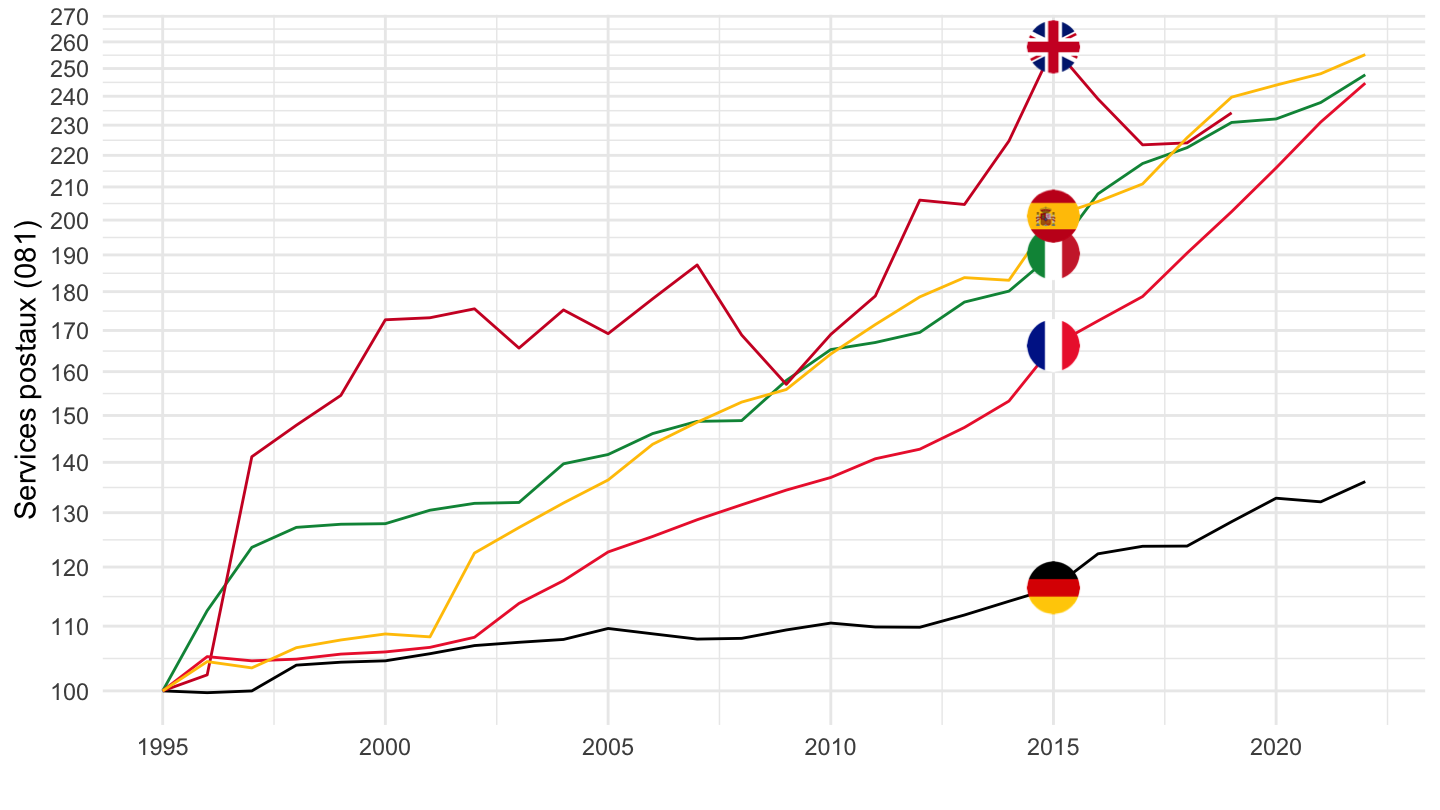
1996-
Code
nama_10_co3_p3 %>%
  filter(unit == "PD15_EUR",
         geo %in% c("FR", "UK", "IT", "DE", "ES"),
         coicop == "CP081") %>%
  left_join(geo, by = "geo") %>%
  year_to_date %>%
  filter(date >= as.Date("1996-01-01")) %>%
  left_join(colors, by = c("Geo" = "country")) %>%
  group_by(Geo) %>%
  mutate(values = 100*values/values[date == as.Date("1996-01-01")]) %>%
  ggplot + geom_line(aes(x = date, y = values, color = color)) +
  theme_minimal()  + add_5flags +
  scale_color_identity() + xlab("") + ylab("Services postaux (081)") +
  scale_x_date(breaks = as.Date(paste0(seq(1960, 2100, 2), "-01-01")),
               labels = date_format("%Y")) +
  theme(legend.position = c(0.2, 0.85),
        legend.title = element_blank()) +
  scale_y_log10(breaks = seq(10, 300, 10))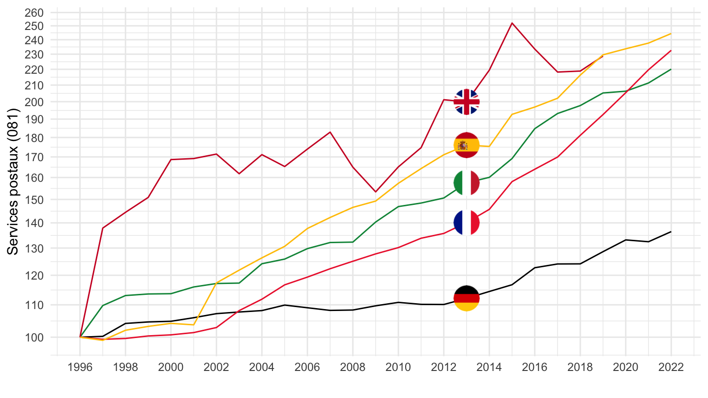
CP09 - Loisirs et culture
1995-
Code
nama_10_co3_p3 %>%
  filter(unit == "PD15_EUR",
         geo %in% c("FR", "NL", "IT", "DE", "ES"),
         coicop == "CP09") %>%
  left_join(geo, by = "geo") %>%
  year_to_date %>%
  filter(date >= as.Date("1995-01-01")) %>%
  left_join(colors, by = c("Geo" = "country")) %>%
  group_by(Geo) %>%
  mutate(values = 100*values/values[date == as.Date("1995-01-01")]) %>%
  ggplot + geom_line(aes(x = date, y = values, color = color)) +
  theme_minimal()  + add_5flags +
  scale_color_identity() + xlab("") + ylab("Loisirs et culture") +
  scale_x_date(breaks = as.Date(paste0(seq(1960, 2100, 5), "-01-01")),
               labels = date_format("%Y")) +
  theme(legend.position = c(0.2, 0.85),
        legend.title = element_blank()) +
  scale_y_log10(breaks = seq(10, 300, 10))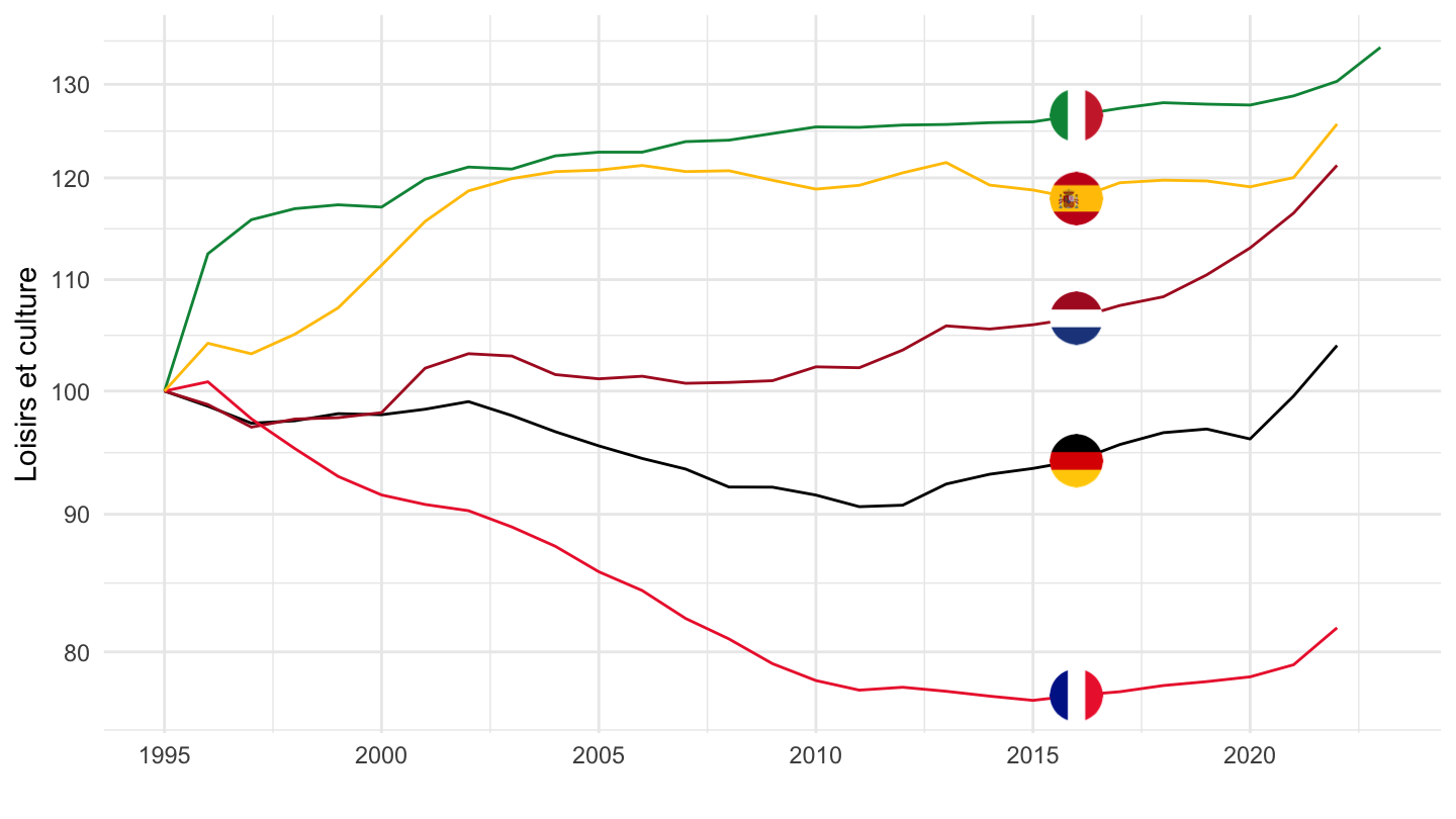
1996-
Code
nama_10_co3_p3 %>%
  filter(unit == "PD15_EUR",
         geo %in% c("FR", "NL", "IT", "DE", "ES"),
         coicop == "CP09") %>%
  left_join(geo, by = "geo") %>%
  year_to_date %>%
  filter(date >= as.Date("1996-01-01")) %>%
  left_join(colors, by = c("Geo" = "country")) %>%
  group_by(Geo) %>%
  mutate(values = 100*values/values[date == as.Date("1996-01-01")]) %>%
  ggplot + geom_line(aes(x = date, y = values, color = color)) +
  theme_minimal()  + add_5flags +
  scale_color_identity() + xlab("") + ylab("Loisirs et culture (CP09)") +
  scale_x_date(breaks = as.Date(paste0(seq(1960, 2100, 2), "-01-01")),
               labels = date_format("%Y")) +
  theme(legend.position = c(0.2, 0.85),
        legend.title = element_blank()) +
  scale_y_log10(breaks = seq(10, 300, 10))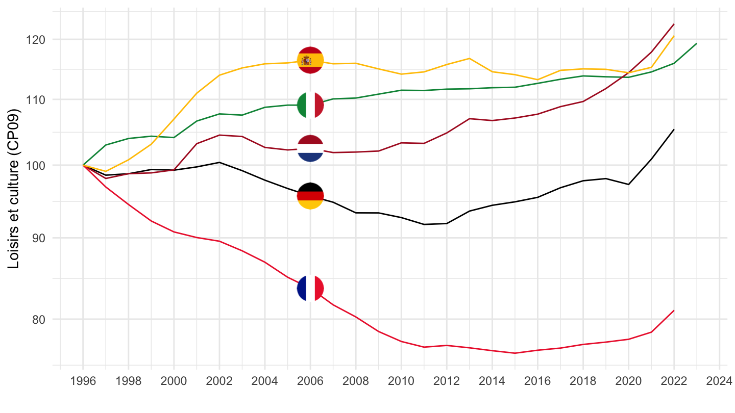
CP08 - Communications
1995-
Code
nama_10_co3_p3 %>%
  filter(unit == "PD15_EUR",
         geo %in% c("FR", "NL", "IT", "DE", "ES"),
         coicop == "CP08") %>%
  left_join(geo, by = "geo") %>%
  year_to_date %>%
  filter(date >= as.Date("1995-01-01"),
         date <= as.Date("2023-01-01")) %>%
  left_join(colors, by = c("Geo" = "country")) %>%
  group_by(Geo) %>%
  mutate(values = 100*values/values[date == as.Date("1995-01-01")]) %>%
  ggplot + geom_line(aes(x = date, y = values, color = color)) +
  theme_minimal()  + add_5flags +
  scale_color_identity() + xlab("") + ylab("Communications (08)") +
  scale_x_date(breaks = as.Date(paste0(seq(1960, 2100, 5), "-01-01")),
               labels = date_format("%Y")) +
  theme(legend.position = c(0.2, 0.85),
        legend.title = element_blank()) +
  scale_y_log10(breaks = seq(10, 300, 10))
1996-
Code
nama_10_co3_p3 %>%
  filter(unit == "PD15_EUR",
         geo %in% c("FR", "NL", "IT", "DE", "ES"),
         coicop == "CP08") %>%
  left_join(geo, by = "geo") %>%
  year_to_date %>%
  filter(date >= as.Date("1996-01-01")) %>%
  left_join(colors, by = c("Geo" = "country")) %>%
  group_by(Geo) %>%
  mutate(values = 100*values/values[date == as.Date("1996-01-01")]) %>%
  ggplot + geom_line(aes(x = date, y = values, color = color)) +
  theme_minimal()  + add_5flags +
  scale_color_identity() + xlab("") + ylab("Communications (08)") +
  scale_x_date(breaks = as.Date(paste0(seq(1960, 2100, 2), "-01-01")),
               labels = date_format("%Y")) +
  theme(legend.position = c(0.2, 0.85),
        legend.title = element_blank()) +
  scale_y_log10(breaks = seq(10, 300, 10))
2000-
Code
nama_10_co3_p3 %>%
  filter(unit == "PD15_EUR",
         geo %in% c("FR", "NL", "IT", "DE", "ES"),
         coicop == "CP08") %>%
  left_join(geo, by = "geo") %>%
  year_to_date %>%
  filter(date >= as.Date("2000-01-01")) %>%
  left_join(colors, by = c("Geo" = "country")) %>%
  group_by(Geo) %>%
  mutate(values = 100*values/values[date == as.Date("2000-01-01")]) %>%
  ggplot + geom_line(aes(x = date, y = values, color = color)) +
  theme_minimal()  + add_5flags +
  scale_color_identity() + xlab("") + ylab("Communications (08)") +
  scale_x_date(breaks = as.Date(paste0(seq(1960, 2100, 2), "-01-01")),
               labels = date_format("%Y")) +
  theme(legend.position = c(0.2, 0.85),
        legend.title = element_blank()) +
  scale_y_log10(breaks = seq(10, 300, 10))
CP071 - Cars
1995-
Code
nama_10_co3_p3 %>%
  filter(unit == "PD15_EUR",
         geo %in% c("FR", "NL", "IT", "DE", "ES"),
         coicop == "CP071") %>%
  left_join(geo, by = "geo") %>%
  year_to_date %>%
  filter(date >= as.Date("1995-01-01")) %>%
  left_join(colors, by = c("Geo" = "country")) %>%
  group_by(Geo) %>%
  mutate(values = 100*values/values[date == as.Date("1995-01-01")]) %>%
  ggplot + geom_line(aes(x = date, y = values, color = color)) +
  theme_minimal()  + add_5flags +
  scale_color_identity() + xlab("") + ylab("") +
  scale_x_date(breaks = as.Date(paste0(seq(1960, 2100, 5), "-01-01")),
               labels = date_format("%Y")) +
  theme(legend.position = c(0.2, 0.85),
        legend.title = element_blank()) +
  scale_y_log10(breaks = seq(10, 300, 10))
1996-
Code
nama_10_co3_p3 %>%
  filter(unit == "PD15_EUR",
         geo %in% c("FR", "NL", "IT", "DE", "ES"),
         coicop == "CP071") %>%
  left_join(geo, by = "geo") %>%
  year_to_date %>%
  filter(date >= as.Date("1996-01-01")) %>%
  left_join(colors, by = c("Geo" = "country")) %>%
  group_by(Geo) %>%
  mutate(values = 100*values/values[date == as.Date("1996-01-01")]) %>%
  ggplot + geom_line(aes(x = date, y = values, color = color)) +
  theme_minimal()  + add_5flags +
  scale_color_identity() + xlab("") + ylab("") +
  scale_x_date(breaks = as.Date(paste0(seq(1960, 2100, 2), "-01-01")),
               labels = date_format("%Y")) +
  theme(legend.position = c(0.2, 0.85),
        legend.title = element_blank()) +
  scale_y_log10(breaks = c(10, 12, 15, 18, 20, seq(10, 300, 10)))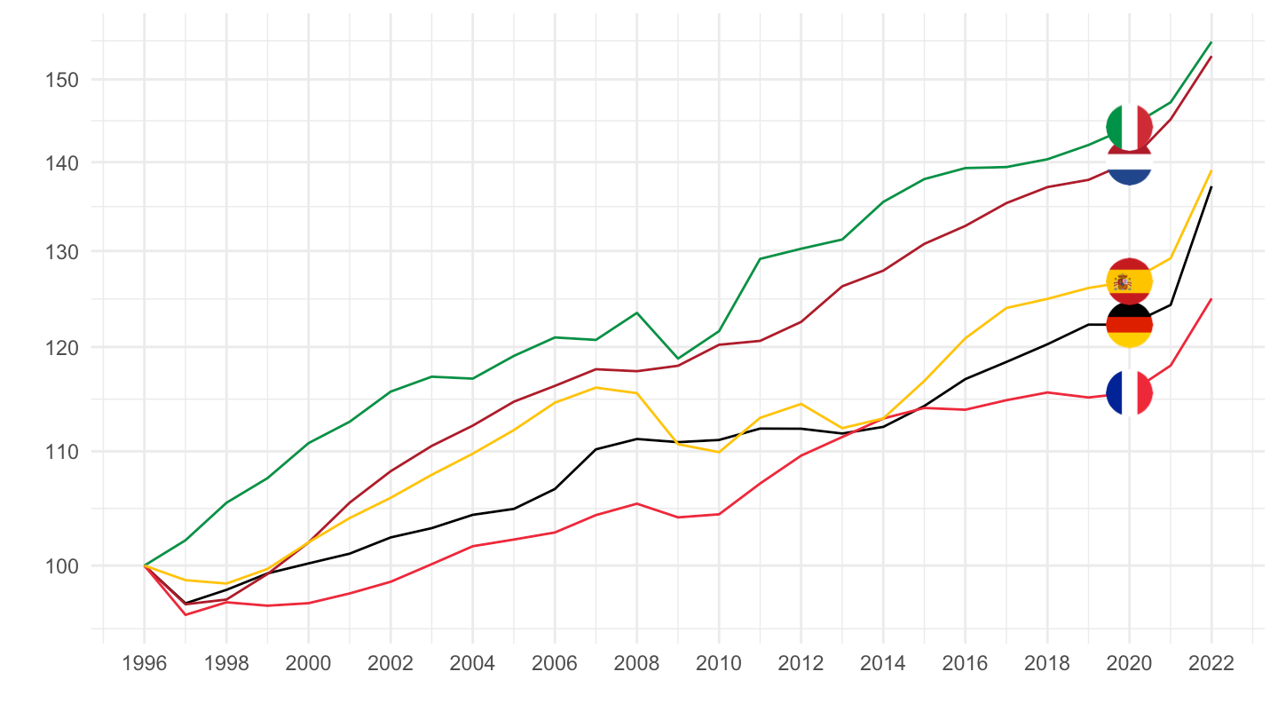
CP091 - Matériel audiovisuel, photographique et de traitement de l’information
1995-
Code
nama_10_co3_p3 %>%
  filter(unit == "PD15_EUR",
         geo %in% c("FR", "NL", "IT", "DE", "ES"),
         coicop == "CP091") %>%
  left_join(geo, by = "geo") %>%
  year_to_date %>%
  filter(date >= as.Date("1995-01-01")) %>%
  left_join(colors, by = c("Geo" = "country")) %>%
  group_by(Geo) %>%
  mutate(values = 100*values/values[date == as.Date("1995-01-01")]) %>%
  ggplot + geom_line(aes(x = date, y = values, color = color)) +
  theme_minimal()  + add_5flags +
  scale_color_identity() + xlab("") + ylab("") +
  scale_x_date(breaks = as.Date(paste0(seq(1960, 2100, 5), "-01-01")),
               labels = date_format("%Y")) +
  theme(legend.position = c(0.2, 0.85),
        legend.title = element_blank()) +
  scale_y_log10(breaks = seq(10, 300, 10))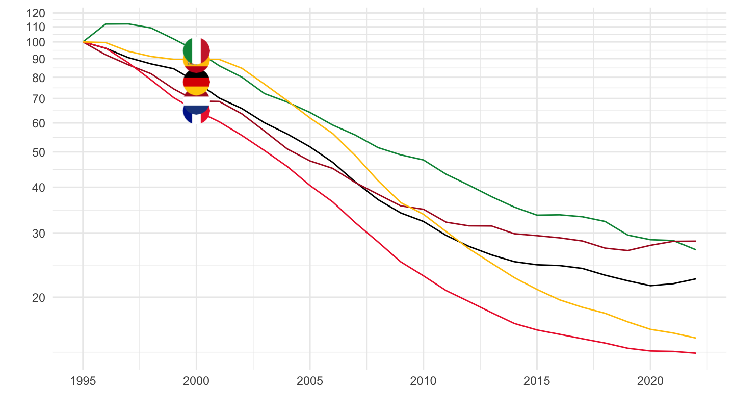
1996-
Code
nama_10_co3_p3 %>%
  filter(unit == "PD15_EUR",
         geo %in% c("FR", "NL", "IT", "DE", "ES"),
         coicop == "CP091") %>%
  left_join(geo, by = "geo") %>%
  year_to_date %>%
  filter(date >= as.Date("1996-01-01")) %>%
  left_join(colors, by = c("Geo" = "country")) %>%
  group_by(Geo) %>%
  mutate(values = 100*values/values[date == as.Date("1996-01-01")]) %>%
  ggplot + geom_line(aes(x = date, y = values, color = color)) +
  theme_minimal()  + add_5flags +
  scale_color_identity() + xlab("") + ylab("") +
  scale_x_date(breaks = as.Date(paste0(seq(1960, 2100, 2), "-01-01")),
               labels = date_format("%Y")) +
  theme(legend.position = c(0.2, 0.85),
        legend.title = element_blank()) +
  scale_y_log10(breaks = c(10, 12, 15, 18, 20, seq(10, 300, 10)))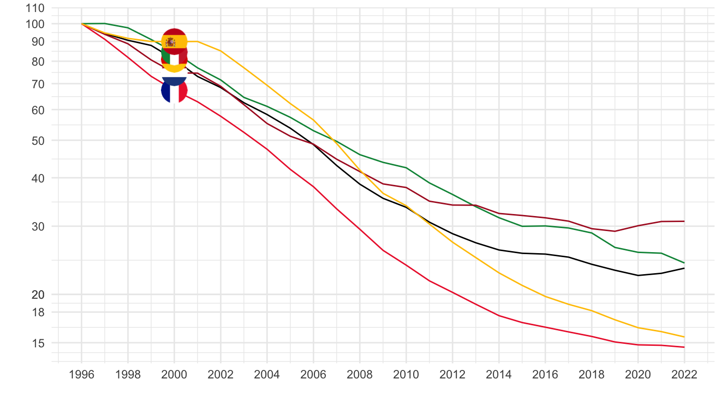
CP082 - Telephone and telefax equipment
1995-
Code
nama_10_co3_p3 %>%
  filter(unit == "PD15_EUR",
         geo %in% c("FR", "UK", "IT", "DE", "ES"),
         coicop == "CP082") %>%
  left_join(geo, by = "geo") %>%
  year_to_date %>%
  filter(date >= as.Date("1995-01-01")) %>%
  left_join(colors, by = c("Geo" = "country")) %>%
  group_by(Geo) %>%
  mutate(values = 100*values/values[date == as.Date("1995-01-01")]) %>%
  ggplot + geom_line(aes(x = date, y = values, color = color)) +
  theme_minimal()  + add_5flags +
  scale_color_identity() + xlab("") + ylab("Matériel de téléphonie et de télécopie (CP082)") +
  scale_x_date(breaks = as.Date(paste0(seq(1960, 2100, 5), "-01-01")),
               labels = date_format("%Y")) +
  theme(legend.position = c(0.2, 0.85),
        legend.title = element_blank()) +
  scale_y_log10(breaks = seq(10, 300, 10))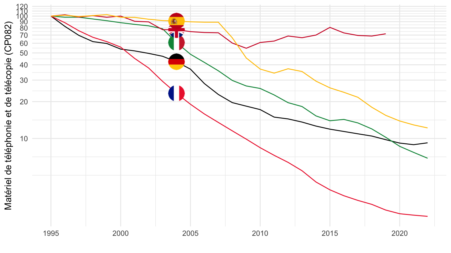
1996-
Code
nama_10_co3_p3 %>%
  filter(unit == "PD15_EUR",
         geo %in% c("FR", "NL", "IT", "DE", "ES"),
         coicop == "CP082") %>%
  left_join(geo, by = "geo") %>%
  year_to_date %>%
  filter(date >= as.Date("1996-01-01")) %>%
  left_join(colors, by = c("Geo" = "country")) %>%
  group_by(Geo) %>%
  mutate(values = 100*values/values[date == as.Date("1996-01-01")]) %>%
  ggplot + geom_line(aes(x = date, y = values, color = color)) +
  theme_minimal()  + add_5flags +
  scale_color_identity() + xlab("") + ylab("Matériel de téléphonie et de télécopie (CP082)") +
  scale_x_date(breaks = as.Date(paste0(seq(1960, 2100, 2), "-01-01")),
               labels = date_format("%Y")) +
  theme(legend.position = c(0.2, 0.85),
        legend.title = element_blank()) +
  scale_y_log10(breaks = c(seq(10, 300, 10), 2, 3, 5, 8))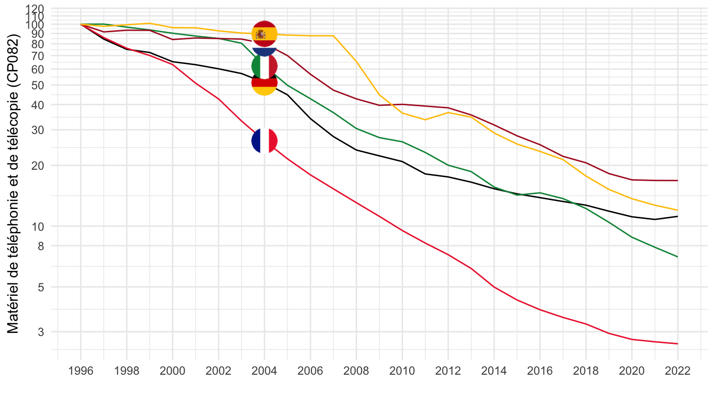
CP083 - Telephone and telefax services
1995-
Code
nama_10_co3_p3 %>%
  filter(unit == "PD15_EUR",
         geo %in% c("FR", "NL", "IT", "DE", "ES"),
         coicop == "CP083") %>%
  left_join(geo, by = "geo") %>%
  year_to_date %>%
  filter(date >= as.Date("1995-01-01")) %>%
  left_join(colors, by = c("Geo" = "country")) %>%
  group_by(Geo) %>%
  mutate(values = 100*values/values[date == as.Date("1995-01-01")]) %>%
  ggplot + geom_line(aes(x = date, y = values, color = color)) +
  theme_minimal()  + add_5flags +
  scale_color_identity() + xlab("") + ylab("Telephone and telefax services (083)") +
  scale_x_date(breaks = as.Date(paste0(seq(1960, 2100, 5), "-01-01")),
               labels = date_format("%Y")) +
  theme(legend.position = c(0.2, 0.85),
        legend.title = element_blank()) +
  scale_y_log10(breaks = seq(10, 300, 10))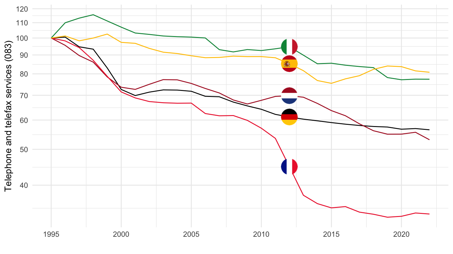
1996-
Code
nama_10_co3_p3 %>%
  filter(unit == "PD15_EUR",
         geo %in% c("FR", "NL", "IT", "DE", "ES"),
         coicop == "CP083") %>%
  left_join(geo, by = "geo") %>%
  year_to_date %>%
  filter(date >= as.Date("1996-01-01")) %>%
  left_join(colors, by = c("Geo" = "country")) %>%
  group_by(Geo) %>%
  mutate(values = 100*values/values[date == as.Date("1996-01-01")]) %>%
  ggplot + geom_line(aes(x = date, y = values, color = color)) +
  theme_minimal()  + add_5flags +
  scale_color_identity() + xlab("") + ylab("Services de téléphonie et de télécopie (083)") +
  scale_x_date(breaks = as.Date(paste0(seq(1960, 2100, 2), "-01-01")),
               labels = date_format("%Y")) +
  theme(legend.position = c(0.2, 0.85),
        legend.title = element_blank()) +
  scale_y_log10(breaks = c(seq(10, 300, 10), 35))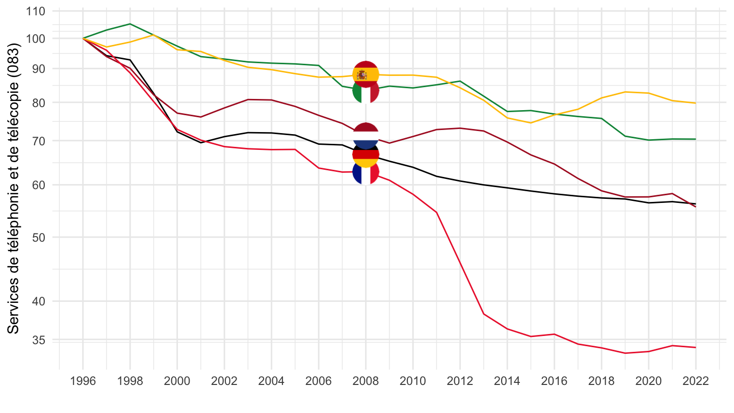
2000-
Code
nama_10_co3_p3 %>%
  filter(unit == "PD15_EUR",
         geo %in% c("FR", "NL", "IT", "DE", "ES"),
         coicop == "CP083") %>%
  left_join(geo, by = "geo") %>%
  year_to_date %>%
  filter(date >= as.Date("2000-01-01")) %>%
  left_join(colors, by = c("Geo" = "country")) %>%
  group_by(Geo) %>%
  mutate(values = 100*values/values[date == as.Date("2000-01-01")]) %>%
  ggplot + geom_line(aes(x = date, y = values, color = color)) +
  theme_minimal()  + add_5flags +
  scale_color_identity() + xlab("") + ylab("Services de téléphonie et de télécopie (083)") +
  scale_x_date(breaks = as.Date(paste0(seq(1960, 2100, 2), "-01-01")),
               labels = date_format("%Y")) +
  theme(legend.position = c(0.2, 0.85),
        legend.title = element_blank()) +
  scale_y_log10(breaks = c(seq(10, 300, 10), 35))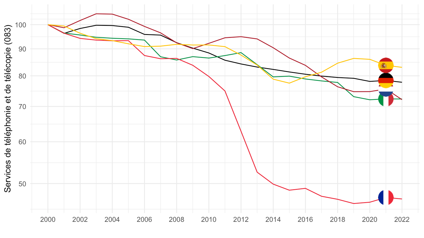
CP056 - Goods and services for routine household maintenance
1995-
Code
nama_10_co3_p3 %>%
  filter(unit == "PD15_EUR",
         geo %in% c("FR", "NL", "IT", "DE", "ES"),
         coicop == "CP056") %>%
  left_join(geo, by = "geo") %>%
  year_to_date %>%
  filter(date >= as.Date("1995-01-01")) %>%
  left_join(colors, by = c("Geo" = "country")) %>%
  group_by(Geo) %>%
  mutate(values = 100*values/values[date == as.Date("1995-01-01")]) %>%
  ggplot + geom_line(aes(x = date, y = values, color = color)) +
  theme_minimal()  + add_5flags +
  scale_color_identity() + xlab("") + ylab("CP053") +
  scale_x_date(breaks = as.Date(paste0(seq(1960, 2100, 5), "-01-01")),
               labels = date_format("%Y")) +
  theme(legend.position = c(0.2, 0.85),
        legend.title = element_blank()) +
  scale_y_log10(breaks = seq(10, 300, 10))
1996-
Code
nama_10_co3_p3 %>%
  filter(unit == "PD15_EUR",
         geo %in% c("FR", "NL", "IT", "DE", "ES"),
         coicop == "CP056") %>%
  left_join(geo, by = "geo") %>%
  year_to_date %>%
  filter(date >= as.Date("1996-01-01")) %>%
  left_join(colors, by = c("Geo" = "country")) %>%
  group_by(Geo) %>%
  mutate(values = 100*values/values[date == as.Date("1996-01-01")]) %>%
  ggplot + geom_line(aes(x = date, y = values, color = color)) +
  theme_minimal()  + add_5flags +
  scale_color_identity() + xlab("") + ylab("CP056") +
  scale_x_date(breaks = as.Date(paste0(seq(1960, 2100, 2), "-01-01")),
               labels = date_format("%Y")) +
  theme(legend.position = c(0.2, 0.85),
        legend.title = element_blank()) +
  scale_y_log10(breaks = c(seq(10, 300, 10), 35))
CP053 - Household appliances
1995-
Code
nama_10_co3_p3 %>%
  filter(unit == "PD15_EUR",
         geo %in% c("FR", "NL", "IT", "DE", "ES"),
         coicop == "CP053") %>%
  left_join(geo, by = "geo") %>%
  year_to_date %>%
  filter(date >= as.Date("1995-01-01")) %>%
  left_join(colors, by = c("Geo" = "country")) %>%
  group_by(Geo) %>%
  mutate(values = 100*values/values[date == as.Date("1995-01-01")]) %>%
  ggplot + geom_line(aes(x = date, y = values, color = color)) +
  theme_minimal()  + add_5flags +
  scale_color_identity() + xlab("") + ylab("CP053") +
  scale_x_date(breaks = as.Date(paste0(seq(1960, 2100, 5), "-01-01")),
               labels = date_format("%Y")) +
  theme(legend.position = c(0.2, 0.85),
        legend.title = element_blank()) +
  scale_y_log10(breaks = seq(10, 300, 10))
1996-
Code
nama_10_co3_p3 %>%
  filter(unit == "PD15_EUR",
         geo %in% c("FR", "NL", "IT", "DE", "ES"),
         coicop == "CP053") %>%
  left_join(geo, by = "geo") %>%
  year_to_date %>%
  filter(date >= as.Date("1996-01-01")) %>%
  left_join(colors, by = c("Geo" = "country")) %>%
  group_by(Geo) %>%
  mutate(values = 100*values/values[date == as.Date("1996-01-01")]) %>%
  ggplot + geom_line(aes(x = date, y = values, color = color)) +
  theme_minimal()  + add_5flags +
  scale_color_identity() + xlab("") + ylab("CP053") +
  scale_x_date(breaks = as.Date(paste0(seq(1960, 2100, 2), "-01-01")),
               labels = date_format("%Y")) +
  theme(legend.position = c(0.2, 0.85),
        legend.title = element_blank()) +
  scale_y_log10(breaks = c(seq(10, 300, 10), 35))
CP126 - Financial services
1995-
Code
nama_10_co3_p3 %>%
  filter(unit == "PD15_EUR",
         geo %in% c("FR", "NL", "IT", "DE", "ES"),
         coicop == "CP126") %>%
  left_join(geo, by = "geo") %>%
  year_to_date %>%
  filter(date >= as.Date("1995-01-01")) %>%
  left_join(colors, by = c("Geo" = "country")) %>%
  group_by(Geo) %>%
  mutate(values = 100*values/values[date == as.Date("1995-01-01")]) %>%
  ggplot + geom_line(aes(x = date, y = values, color = color)) +
  theme_minimal()  + add_5flags +
  scale_color_identity() + xlab("") + ylab("") +
  scale_x_date(breaks = as.Date(paste0(seq(1960, 2100, 5), "-01-01")),
               labels = date_format("%Y")) +
  theme(legend.position = c(0.2, 0.85),
        legend.title = element_blank()) +
  scale_y_log10(breaks = seq(10, 300, 10))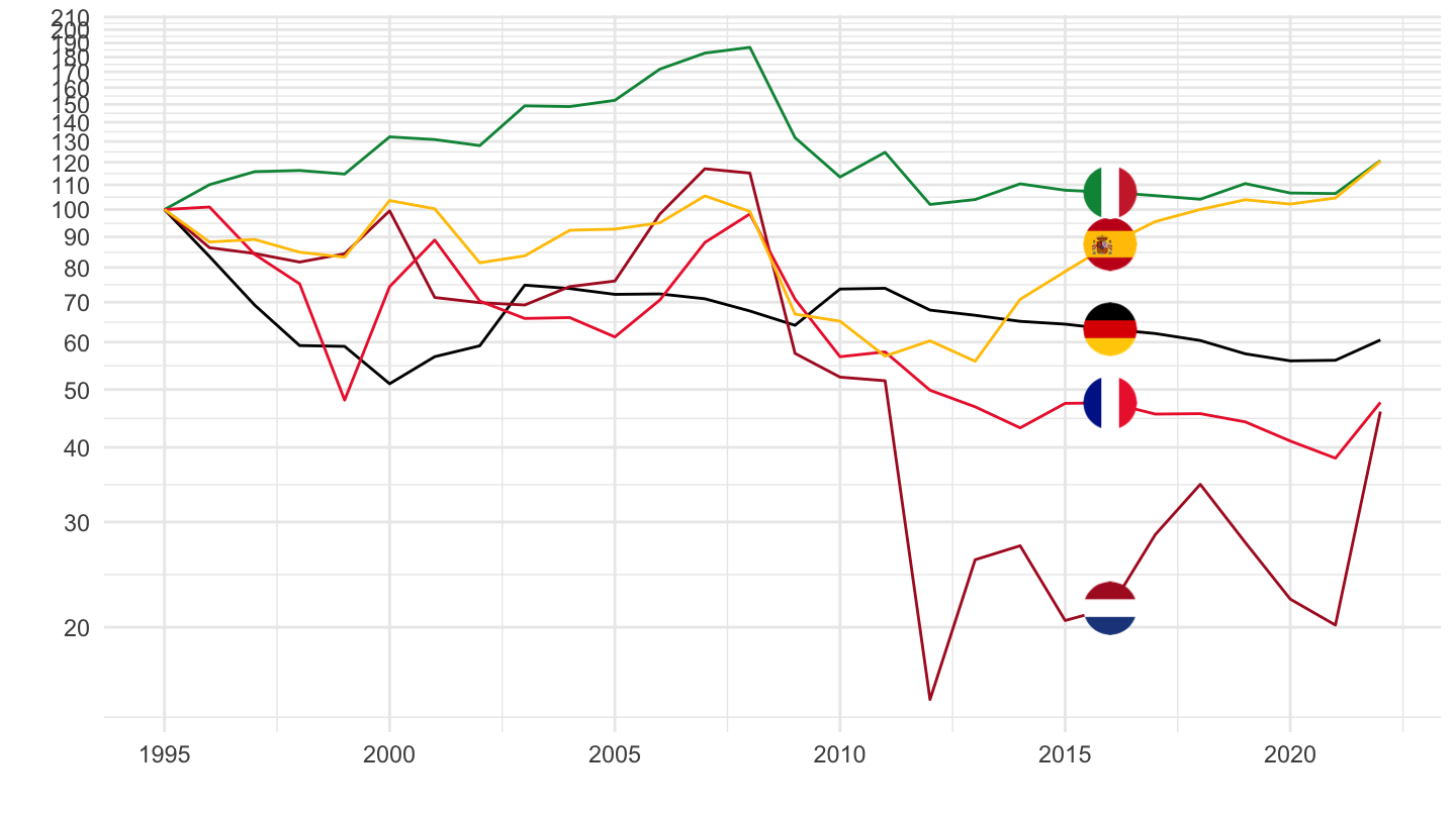
1996-
Code
nama_10_co3_p3 %>%
  filter(unit == "PD15_EUR",
         geo %in% c("FR", "NL", "IT", "DE", "ES"),
         coicop == "CP126") %>%
  left_join(geo, by = "geo") %>%
  year_to_date %>%
  filter(date >= as.Date("1996-01-01")) %>%
  left_join(colors, by = c("Geo" = "country")) %>%
  group_by(Geo) %>%
  mutate(values = 100*values/values[date == as.Date("1996-01-01")]) %>%
  ggplot + geom_line(aes(x = date, y = values, color = color)) +
  theme_minimal()  + add_5flags +
  scale_color_identity() + xlab("") + ylab("") +
  scale_x_date(breaks = as.Date(paste0(seq(1960, 2100, 5), "-01-01")),
               labels = date_format("%Y")) +
  theme(legend.position = c(0.2, 0.85),
        legend.title = element_blank()) +
  scale_y_log10(breaks = seq(10, 300, 10))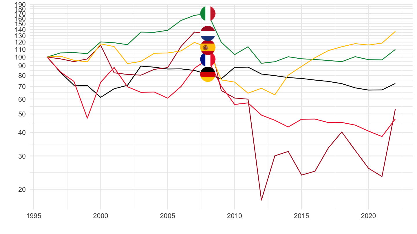
CP061 - Medical products, appliances and equipment
1995-
Code
nama_10_co3_p3 %>%
  filter(unit == "PD15_EUR",
         geo %in% c("FR", "NL", "IT", "DE", "ES"),
         coicop == "CP061") %>%
  left_join(geo, by = "geo") %>%
  year_to_date %>%
  filter(date >= as.Date("1995-01-01")) %>%
  left_join(colors, by = c("Geo" = "country")) %>%
  group_by(Geo) %>%
  mutate(values = 100*values/values[date == as.Date("1995-01-01")]) %>%
  ggplot + geom_line(aes(x = date, y = values, color = color)) +
  theme_minimal()  + add_5flags +
  scale_color_identity() + xlab("") + ylab("") +
  scale_x_date(breaks = as.Date(paste0(seq(1960, 2100, 5), "-01-01")),
               labels = date_format("%Y")) +
  theme(legend.position = c(0.2, 0.85),
        legend.title = element_blank()) +
  scale_y_log10(breaks = seq(10, 300, 10))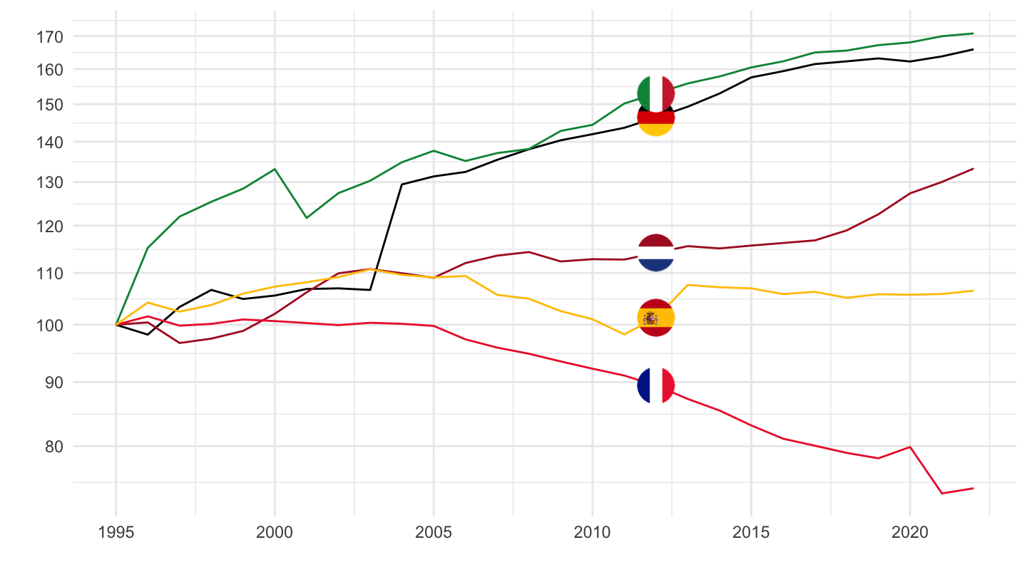
1996-
Code
nama_10_co3_p3 %>%
  filter(unit == "PD15_EUR",
         geo %in% c("FR", "NL", "IT", "DE", "ES"),
         coicop == "CP061") %>%
  left_join(geo, by = "geo") %>%
  year_to_date %>%
  filter(date >= as.Date("1995-01-01")) %>%
  left_join(colors, by = c("Geo" = "country")) %>%
  group_by(Geo) %>%
  mutate(values = 100*values/values[date == as.Date("1996-01-01")]) %>%
  filter(date >= as.Date("1996-01-01")) %>%
  ggplot + geom_line(aes(x = date, y = values, color = color)) +
  theme_minimal()  + add_5flags +
  scale_color_identity() + xlab("") + ylab("Loyers fictifs") +
  scale_x_date(breaks = as.Date(paste0(seq(1960, 2100, 2), "-01-01")),
               labels = date_format("%Y")) +
  theme(legend.position = c(0.2, 0.85),
        legend.title = element_blank()) +
  scale_y_log10(breaks = seq(10, 300, 10))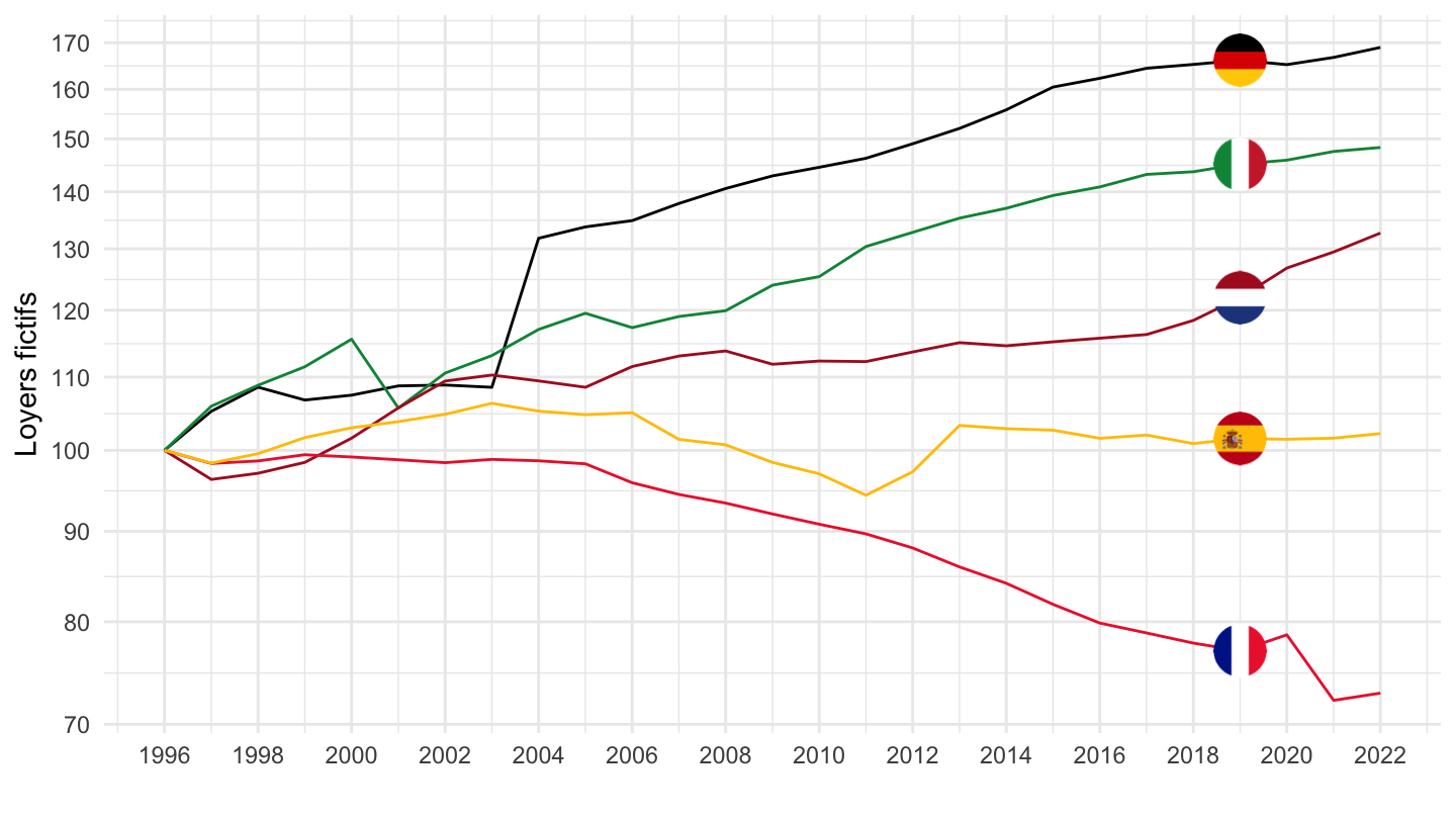
CP042 - Imputed rentals for housing
1995-
Code
nama_10_co3_p3 %>%
  filter(unit == "PD15_EUR",
         geo %in% c("FR", "NL", "IT", "DE", "ES"),
         coicop == "CP042") %>%
  left_join(geo, by = "geo") %>%
  year_to_date %>%
  filter(date >= as.Date("1995-01-01")) %>%
  left_join(colors, by = c("Geo" = "country")) %>%
  group_by(Geo) %>%
  mutate(values = 100*values/values[date == as.Date("1995-01-01")]) %>%
  ggplot + geom_line(aes(x = date, y = values, color = color)) +
  theme_minimal()  + add_5flags +
  scale_color_identity() + xlab("") + ylab("") +
  scale_x_date(breaks = as.Date(paste0(seq(1960, 2100, 5), "-01-01")),
               labels = date_format("%Y")) +
  theme(legend.position = c(0.2, 0.85),
        legend.title = element_blank()) +
  scale_y_log10(breaks = seq(10, 300, 10))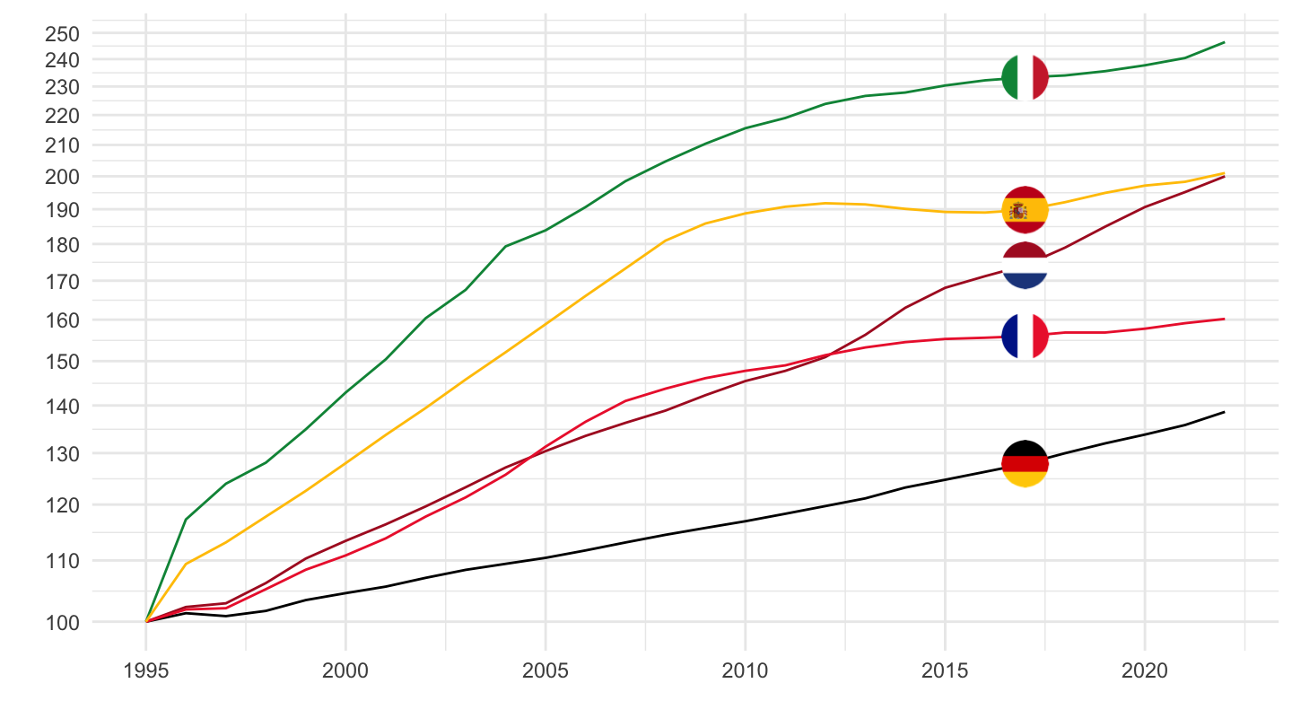
1996-
Code
nama_10_co3_p3 %>%
  filter(unit == "PD15_EUR",
         geo %in% c("FR", "NL", "IT", "DE", "ES"),
         coicop == "CP042") %>%
  left_join(geo, by = "geo") %>%
  year_to_date %>%
  filter(date >= as.Date("1995-01-01")) %>%
  left_join(colors, by = c("Geo" = "country")) %>%
  group_by(Geo) %>%
  mutate(values = 100*values/values[date == as.Date("1996-01-01")]) %>%
  filter(date >= as.Date("1996-01-01")) %>%
  ggplot + geom_line(aes(x = date, y = values, color = color)) +
  theme_minimal()  + add_5flags +
  scale_color_identity() + xlab("") + ylab("Loyers fictifs") +
  scale_x_date(breaks = as.Date(paste0(seq(1960, 2100, 2), "-01-01")),
               labels = date_format("%Y")) +
  theme(legend.position = c(0.2, 0.85),
        legend.title = element_blank()) +
  scale_y_log10(breaks = seq(10, 300, 10))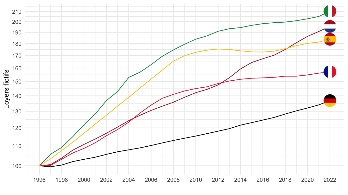
CP041 - Actual rentals for housing
1995-
Code
nama_10_co3_p3 %>%
  filter(unit == "PD15_EUR",
         geo %in% c("FR", "NL", "IT", "DE", "ES"),
         coicop == "CP041") %>%
  left_join(geo, by = "geo") %>%
  year_to_date %>%
  filter(date >= as.Date("1995-01-01")) %>%
  left_join(colors, by = c("Geo" = "country")) %>%
  group_by(Geo) %>%
  mutate(values = 100*values/values[date == as.Date("1995-01-01")]) %>%
  ggplot + geom_line(aes(x = date, y = values, color = color)) +
  theme_minimal()  + add_5flags +
  scale_color_identity() + xlab("") + ylab("") +
  scale_x_date(breaks = as.Date(paste0(seq(1960, 2100, 5), "-01-01")),
               labels = date_format("%Y")) +
  theme(legend.position = c(0.2, 0.85),
        legend.title = element_blank()) +
  scale_y_log10(breaks = seq(10, 300, 10))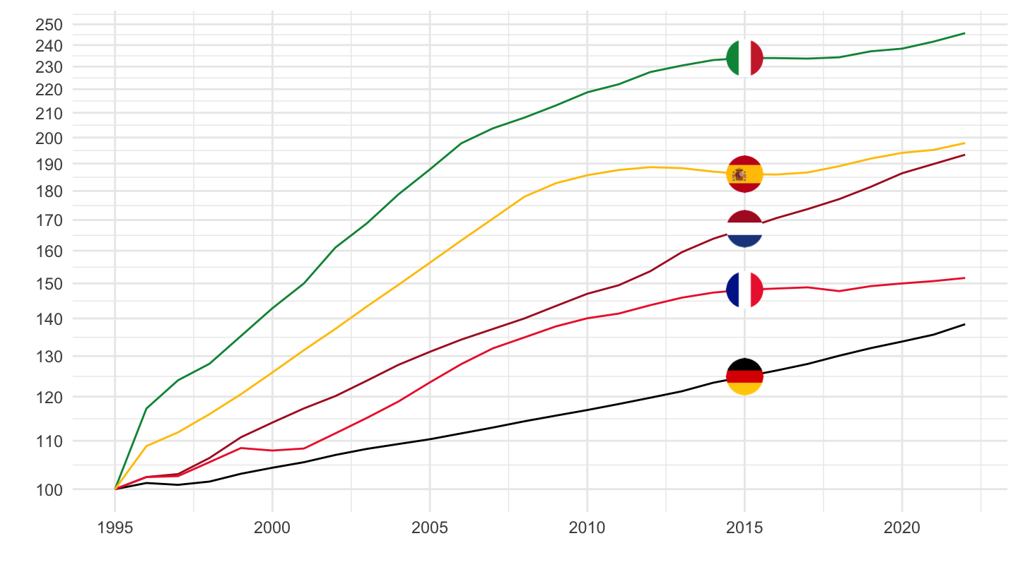
1996-
Code
nama_10_co3_p3 %>%
  filter(unit == "PD15_EUR",
         geo %in% c("FR", "NL", "IT", "DE", "ES"),
         coicop == "CP041") %>%
  left_join(geo, by = "geo") %>%
  year_to_date %>%
  filter(date >= as.Date("1996-01-01")) %>%
  left_join(colors, by = c("Geo" = "country")) %>%
  group_by(Geo) %>%
  mutate(values = 100*values/values[date == as.Date("1996-01-01")]) %>%
  ggplot + geom_line(aes(x = date, y = values, color = color)) +
  theme_minimal()  + add_5flags +
  scale_color_identity() + xlab("") + ylab("") +
  scale_x_date(breaks = as.Date(paste0(seq(1960, 2100, 2), "-01-01")),
               labels = date_format("%Y")) +
  theme(legend.position = c(0.2, 0.85),
        legend.title = element_blank()) +
  scale_y_log10(breaks = seq(10, 300, 10))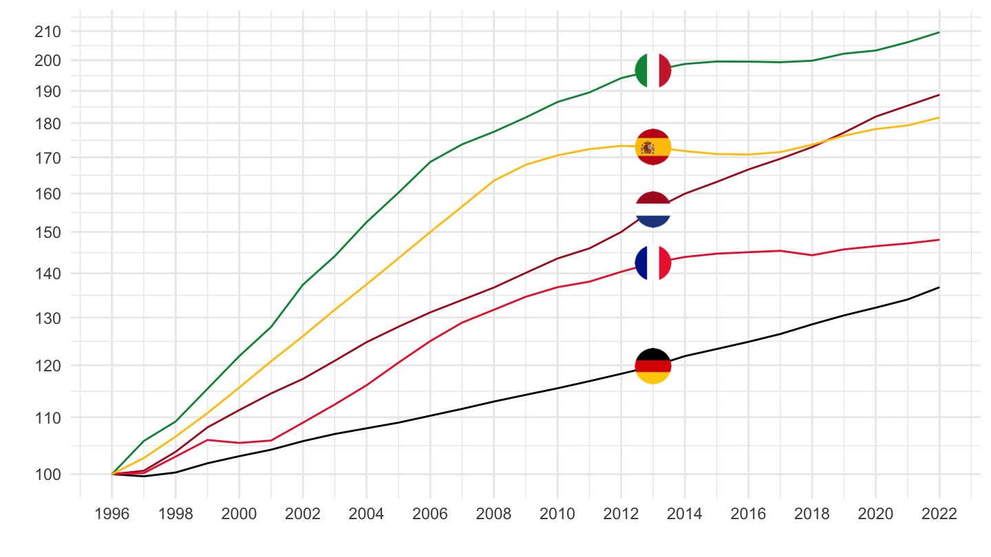
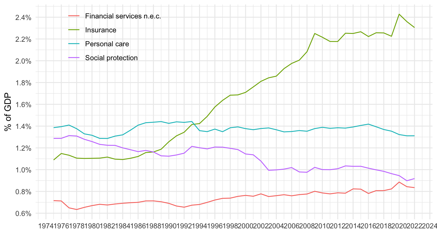
Housing
% of GDP
Code
nama_10_co3_p3 %>%
  filter(unit == "CLV10_MEUR",
         time == "2017",
         grepl("CP04", coicop)) %>%
  left_join(nama_10_gdp %>%
              filter(na_item == "B1GQ",
                     unit == "CLV10_MEUR") %>%
              select(geo, time, gdp = values),
            by = c("geo", "time")) %>%
  mutate(values = round(100*values/gdp, 2)) %>%
  left_join(geo, by = "geo") %>%
  select(geo, Geo, coicop, values, coicop) %>%
  spread(coicop, values) %>%
  mutate(Geo = ifelse(geo == "DE", "Germany", Geo)) %>%
  mutate(Flag = gsub(" ", "-", str_to_lower(Geo)),
         Flag = paste0('<img src="../../bib/flags/vsmall/', Flag, '.png" alt="Flag">')) %>%
  select(Flag, everything()) %>%
  {if (is_html_output()) datatable(., filter = 'top', rownames = F, escape = F) else .}
% of GDP
Code
nama_10_co3_p3 %>%
  filter(unit == "CLV10_MEUR",
         time == "2017",
         grepl("CP04", coicop)) %>%
  left_join(nama_10_gdp %>%
              filter(na_item == "B1GQ",
                     unit == "CLV10_MEUR") %>%
              select(geo, time, gdp = values),
            by = c("geo", "time")) %>%
  left_join(geo, by = "geo") %>%
  left_join(tibble(coicop = c("CP04", "CP041", "CP042",
                              "CP043", "CP044", "CP045"),
                   Coicop = c("Housing", "Actual rents", "Imputed rents",
                              "Maintainance", "Electricity", "Water")),
            by = "coicop") %>%
  mutate(values = round(100*values/gdp, 2)) %>%
  select(geo, Geo, Coicop, values) %>%
  spread(Coicop, values) %>%
  transmute(geo, Geo, Housing, `Actual rents`, `Imputed rents`,
            `Other` = `Maintainance` + `Water` + Electricity) %>%
  arrange(-`Imputed rents`) %>%
  mutate(Geo = ifelse(geo == "DE", "Germany", Geo)) %>%
  mutate(Flag = gsub(" ", "-", str_to_lower(Geo)),
         Flag = paste0('<img src="../../bib/flags/vsmall/', Flag, '.png" alt="Flag">')) %>%
  select(Flag, everything()) %>%
  {if (is_html_output()) datatable(., filter = 'top', rownames = F, escape = F) else .}
% of Aggregate Consumption
Code
nama_10_co3_p3 %>%
  filter(unit == "CLV10_MEUR",
         time == "2017",
         grepl("CP04", coicop)) %>%
  left_join(nama_10_co3_p3 %>%
              filter(coicop == "TOTAL",
                     unit == "CLV10_MEUR") %>%
              select(geo, time, aggregate_c = values),
            by = c("geo", "time")) %>%
  left_join(geo, by = "geo") %>%
  left_join(tibble(coicop = c("CP04", "CP041", "CP042",
                              "CP043", "CP044", "CP045"),
                   Coicop = c("Housing", "Actual rents", "Imputed rents",
                              "Maintainance", "Electricity", "Water")),
            by = "coicop") %>%
  mutate(values = round(100*values/aggregate_c, 2)) %>%
  select(geo, Geo, Coicop, values) %>%
  spread(Coicop, values) %>%
  transmute(geo, Geo, `All rents` = `Actual rents` + `Imputed rents`,
            `Actual rents`, `Imputed rents`,
            `Other` = `Maintainance` + `Water` + Electricity) %>%
  arrange(-`All rents`) %>%
  mutate(Geo = ifelse(geo == "DE", "Germany", Geo)) %>%
  mutate(Flag = gsub(" ", "-", str_to_lower(Geo)),
         Flag = paste0('<img src="../../bib/flags/vsmall/', Flag, '.png" alt="Flag">')) %>%
  select(Flag, everything()) %>%
  {if (is_html_output()) datatable(., filter = 'top', rownames = F, escape = F) else .}
% of Aggregate Consumption
png
Code
library(gt)
library(gtExtras)
table1 <- nama_10_co3_p3 %>%
  filter(unit == "CP_MEUR",
         time == "2020",
         grepl("CP04", coicop),
         !(geo %in% c("EU27_2020", "EU28", "EA12", "EA", "EA19", "EU15"))) %>%
  filter(geo %in% c("BE", "DE", "EE", "IE", "GR", "ES", "FR", "IT", "CY",
                    "LV", "LT", "LU", "MT", "NL", "AT", "PT", "SI", "SK", "FI")) %>%
  left_join(nama_10_co3_p3 %>%
              filter(coicop == "TOTAL",
                     unit == "CP_MEUR") %>%
              select(geo, time, aggregate_c = values),
            by = c("geo", "time")) %>%
  left_join(geo, by = "geo") %>%
  left_join(tibble(coicop = c("CP04", "CP041", "CP042", "CP043", "CP044", "CP045"),
                   Coicop = c("Housing", "Actual rents", "Imputed rents", "Maintainance", "Electricity", "Water")),
            by = "coicop") %>%
  mutate(values = round(100*values/aggregate_c, 1),
         Geo = ifelse(geo == "DE", "Germany", Geo)) %>%
  select(geo, Geo, Coicop, values) %>%
  spread(Coicop, values) %>%
  transmute(geo, Geo, Housing, `Actual rents`, `Imputed rents`,
            `All rents` = `Actual rents` + `Imputed rents`,
            `Other` = `Maintainance` + `Water` + Electricity) %>%
  arrange(-`Housing`) %>%
  mutate(geo = ifelse(geo == "EL", "GR", geo),
         geo = ifelse(geo == "UK", "GB", geo)) %>%
  gt() %>%
  fmt_number(columns = 3:7 , locale = "fr", decimals = 1, pattern = "{x}%") |>
  cols_align(align = "center", columns = 3:7) |>
  fmt_flag(columns = geo, height = "1.5em") %>%
  cols_width(3:7 ~ px(50)) |>
  gt_theme_538()


gtsave(table1, filename = "nama_10_co3_p3_files/figure-html/table1.png")
i_g("data/eurostat/nama_10_co3_p3_files/figure-html/table1.png")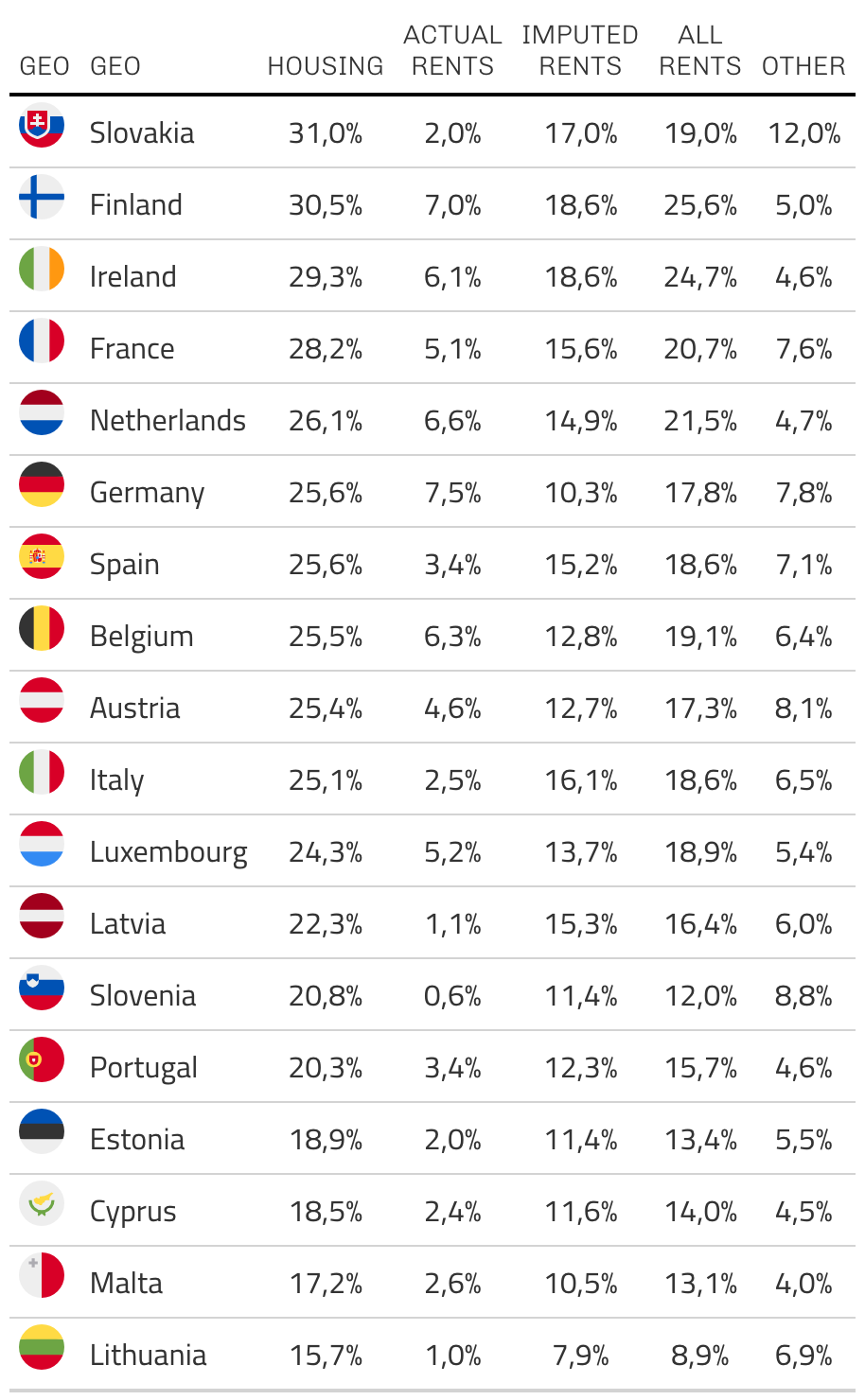
Code
include_graphics3b("bib/eurostat/nama_10_co3_p3_ex1-0.png")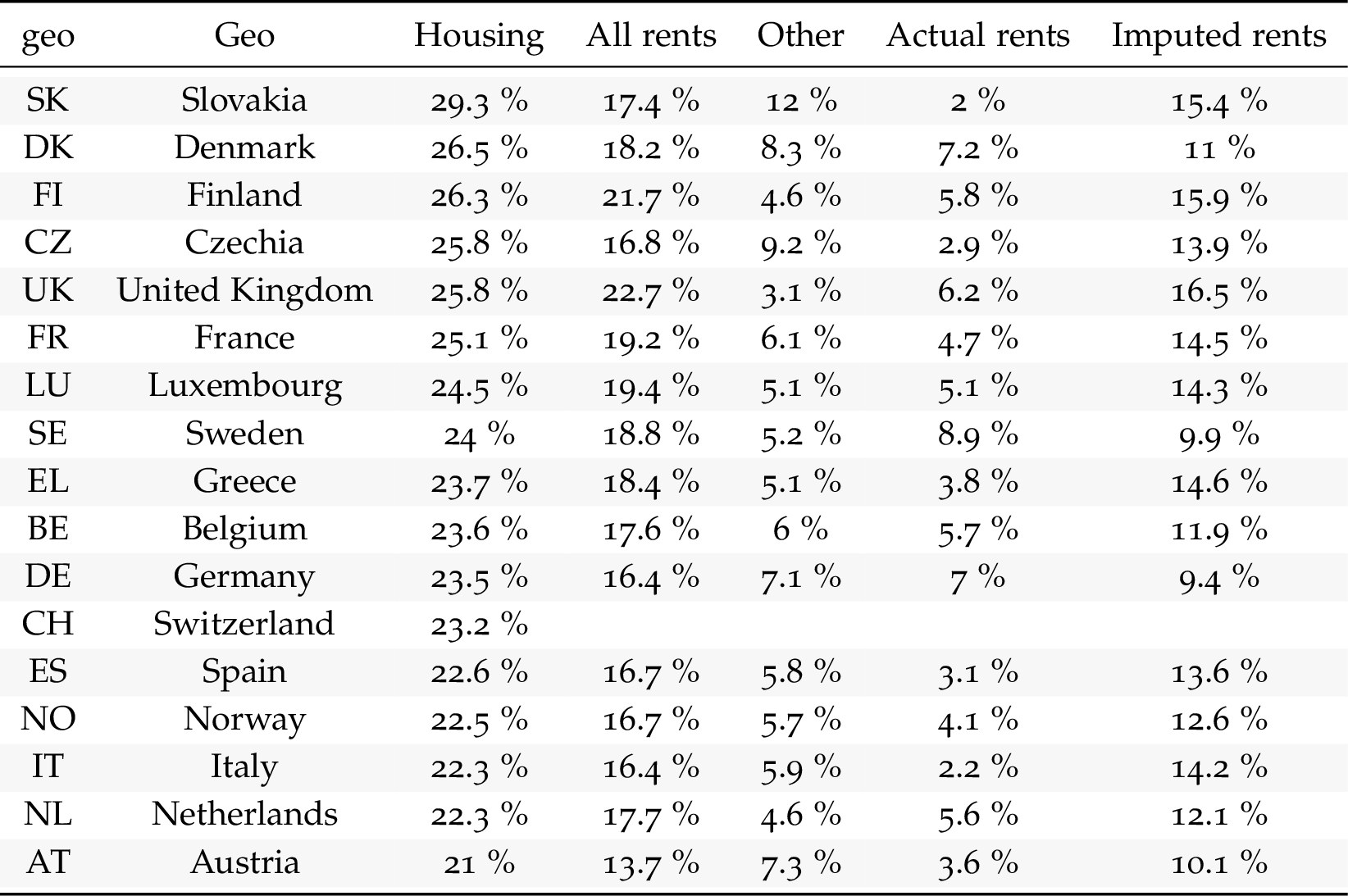
Code
include_graphics3b("bib/eurostat/nama_10_co3_p3_ex1-1.png")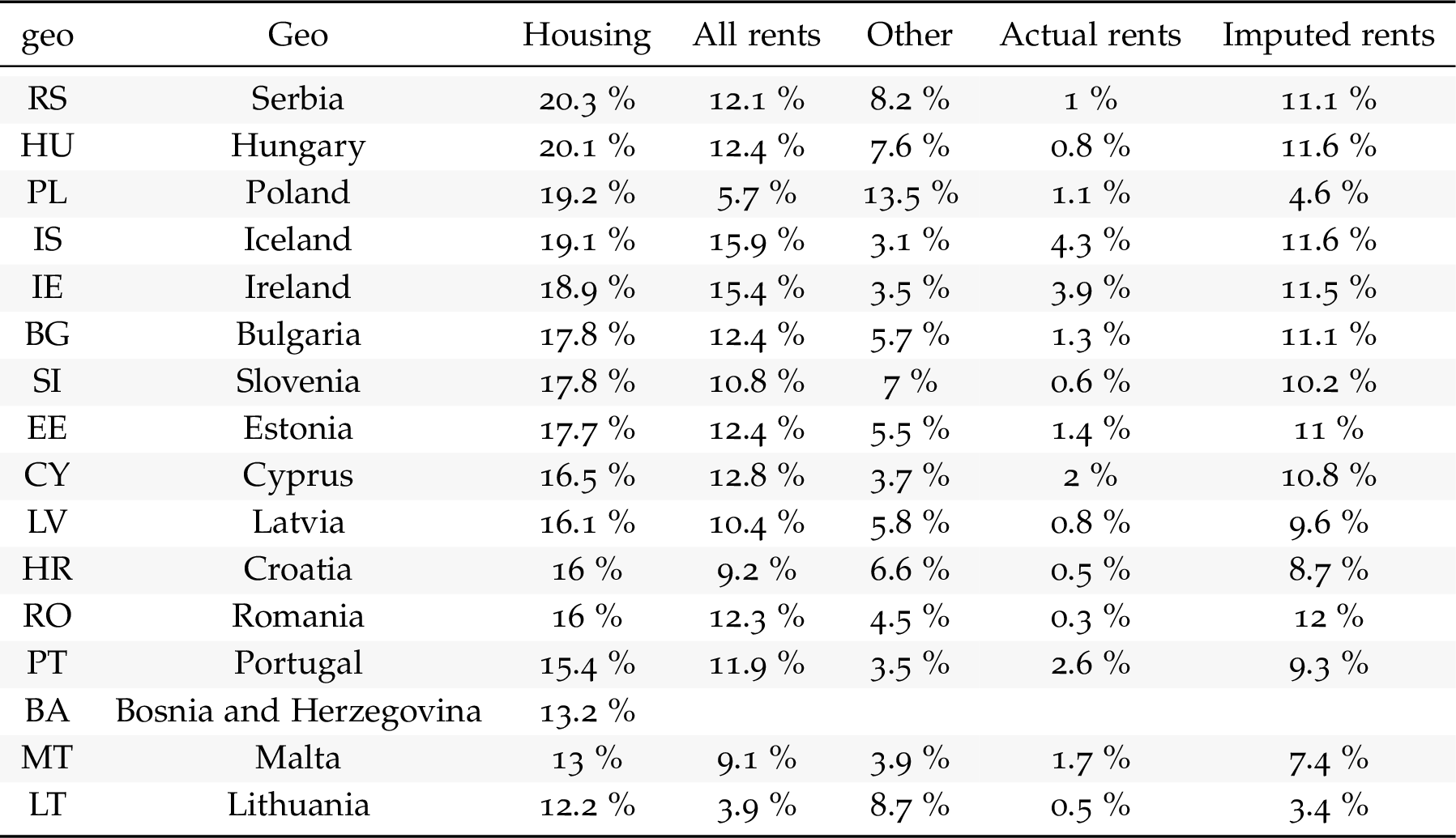
Javascript
Code
nama_10_co3_p3 %>%
  filter(unit == "CLV10_MEUR",
         time == "2018",
         grepl("CP04", coicop)) %>%
  left_join(nama_10_co3_p3 %>%
              filter(coicop == "TOTAL",
                     unit == "CLV10_MEUR") %>%
              select(geo, time, aggregate_c = values),
            by = c("geo", "time")) %>%
  left_join(geo, by = "geo") %>%
  left_join(tibble(coicop = c("CP04", "CP041", "CP042",
                              "CP043", "CP044", "CP045"),
                   Coicop = c("Housing", "Actual rents", "Imputed rents",
                              "Maintainance", "Electricity", "Water")),
            by = "coicop") %>%
  mutate(values = round(100*values/aggregate_c, 1)) %>%
  select(geo, Geo, Coicop, values) %>%
  spread(Coicop, values) %>%
  transmute(geo, Geo, Housing, `All rents` = `Actual rents` + `Imputed rents`,
            `Actual rents`, `Imputed rents`,
            `Other` = `Maintainance` + `Water` + Electricity) %>%
  arrange(-`All rents`) %>%
  mutate(Geo = ifelse(geo == "DE", "Germany", Geo)) %>%
  mutate(Flag = gsub(" ", "-", str_to_lower(Geo)),
         Flag = paste0('<img src="../../bib/flags/vsmall/', Flag, '.png" alt="Flag">')) %>%
  select(Flag, everything()) %>%
  {if (is_html_output()) datatable(., filter = 'top', rownames = F, escape = F) else .}
Table
62 Items
Code
nama_10_co3_p3 %>%
  filter(unit == "CLV10_MEUR",
         time == "2017",
         geo %in% c("FR", "UK", "ES", "IT")) %>%
  left_join(nama_10_gdp %>%
              filter(na_item == "B1GQ",
                     unit == "CLV10_MEUR") %>%
              select(geo, time, gdp = values),
            by = c("geo", "time")) %>%
  mutate(values = round(100*values/gdp, 2)) %>%
  left_join(geo, by = "geo") %>%
  select(Geo, values, coicop) %>%
  left_join(coicop, by = "coicop") %>%
  spread(Geo, values) %>%
  {if (is_html_output()) datatable(., filter = 'top', rownames = F) else .}
2 Digit - 12 Items
Code
nama_10_co3_p3 %>%
  filter(unit == "CLV10_MEUR",
         time == "2017",
         geo %in% c("FR", "UK", "ES", "IT"),
         nchar(coicop) == 4) %>%
  left_join(nama_10_gdp %>%
              filter(na_item == "B1GQ",
                     unit == "CLV10_MEUR") %>%
              select(geo, time, gdp = values),
            by = c("geo", "time")) %>%
  mutate(values = round(100*values/gdp, 2)) %>%
  left_join(geo, by = "geo") %>%
  select(Geo, values, coicop) %>%
  left_join(coicop, by = "coicop") %>%
  spread(Geo, values) %>%
  arrange(-`France`) %>%
  {if (is_html_output()) datatable(., filter = 'top', rownames = F) else .}
3 Digit - 48 Items
Code
nama_10_co3_p3 %>%
  filter(unit == "CLV10_MEUR",
         time == "2017",
         geo %in% c("FR", "UK", "ES", "IT"),
         nchar(coicop) == 5) %>%
  left_join(nama_10_gdp %>%
              filter(na_item == "B1GQ",
                     unit == "CLV10_MEUR") %>%
              select(geo, time, gdp = values),
            by = c("geo", "time")) %>%
  mutate(values = round(100*values/gdp, 2)) %>%
  left_join(geo, by = "geo") %>%
  select(Geo, values, coicop) %>%
  left_join(coicop, by = "coicop") %>%
  spread(Geo, values) %>%
  {if (is_html_output()) datatable(., filter = 'top', rownames = F) else .}
France, Italy, United Kingdom, Spain, Germany
TOTAL consumption
Real
Code
nama_10_co3_p3 %>%
  filter(unit == "CLV10_MEUR",
         geo %in% c("FR", "NL", "IT", "ES", "DE"),
         coicop == "TOTAL") %>%
  left_join(nama_10_gdp %>%
              filter(na_item == "B1GQ",
                     unit == "CLV10_MEUR") %>%
              select(geo, time, gdp = values),
            by = c("geo", "time")) %>%
  left_join(geo, by = "geo") %>%
  year_to_date %>%
  filter(date >= as.Date("1995-01-01")) %>%
  left_join(colors, by = c("Geo" = "country")) %>%
  mutate(values = values/gdp) %>%
  ggplot + geom_line(aes(x = date, y = values, color = color)) +
  theme_minimal()  + add_5flags +
  scale_color_identity() + xlab("") + ylab("% of GDP") +
  scale_x_date(breaks = as.Date(paste0(seq(1960, 2100, 5), "-01-01")),
               labels = date_format("%Y")) +
  theme(legend.position = c(0.2, 0.85),
        legend.title = element_blank()) +
  scale_y_continuous(breaks = 0.01*seq(0, 200, 1),
                     labels = scales::percent_format(accuracy = 1))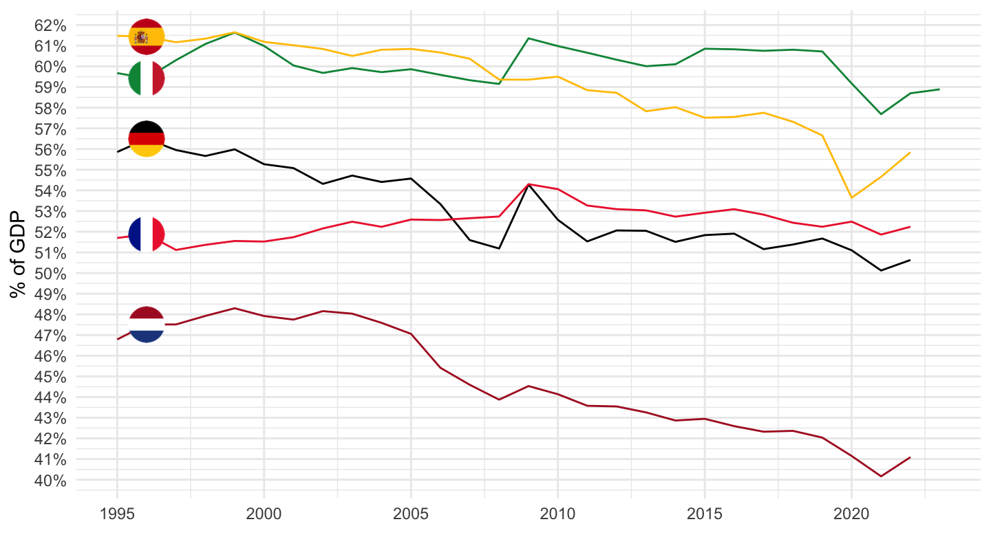
Nominal
Code
nama_10_co3_p3 %>%
  filter(unit == "CP_MEUR",
         geo %in% c("FR", "UK", "IT", "ES", "DE"),
         coicop == "TOTAL") %>%
  left_join(nama_10_gdp %>%
              filter(na_item == "B1GQ",
                     unit == "CP_MEUR") %>%
              select(geo, time, gdp = values),
            by = c("geo", "time")) %>%
  left_join(geo, by = "geo") %>%
  year_to_date %>%
  filter(date >= as.Date("1995-01-01")) %>%
  left_join(colors, by = c("Geo" = "country")) %>%
  mutate(values = values/gdp) %>%
  ggplot + geom_line(aes(x = date, y = values, color = color)) +
  theme_minimal()  + add_5flags +
  scale_color_identity() + xlab("") + ylab("% of GDP") +
  scale_x_date(breaks = as.Date(paste0(seq(1960, 2100, 5), "-01-01")),
               labels = date_format("%Y")) +
  theme(legend.position = c(0.2, 0.85),
        legend.title = element_blank()) +
  scale_y_continuous(breaks = 0.01*seq(0, 200, 1),
                     labels = scales::percent_format(accuracy = 1))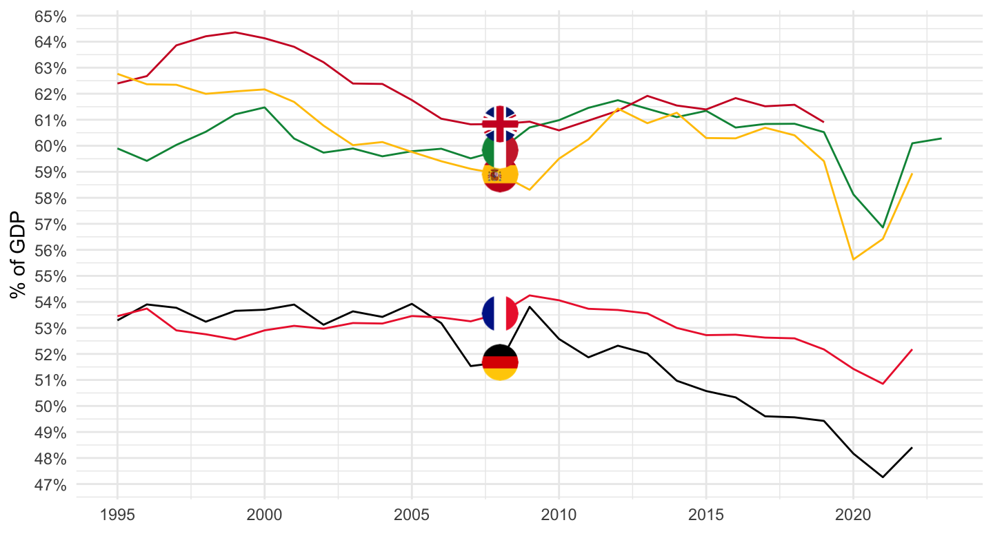
CP041
Nominal
Code
nama_10_co3_p3 %>%
  filter(unit == "CP_MEUR",
         geo %in% c("FR", "UK", "IT", "ES", "DE"),
         coicop == "CP041") %>%
  left_join(nama_10_gdp %>%
              filter(na_item == "B1GQ",
                     unit == "CP_MEUR") %>%
              select(geo, time, gdp = values),
            by = c("geo", "time")) %>%
  left_join(geo, by = "geo") %>%
  year_to_date %>%
  filter(date >= as.Date("1995-01-01")) %>%
  left_join(colors, by = c("Geo" = "country")) %>%
  mutate(values = values/gdp) %>%
  ggplot + geom_line(aes(x = date, y = values, color = color)) +
  theme_minimal()  + add_5flags +
  scale_color_identity() + xlab("") + ylab("% of GDP") +
  scale_x_date(breaks = as.Date(paste0(seq(1960, 2100, 5), "-01-01")),
               labels = date_format("%Y")) +
  theme(legend.position = c(0.2, 0.85),
        legend.title = element_blank()) +
  scale_y_continuous(breaks = 0.01*seq(0, 200, .1),
                     labels = scales::percent_format(accuracy = .1))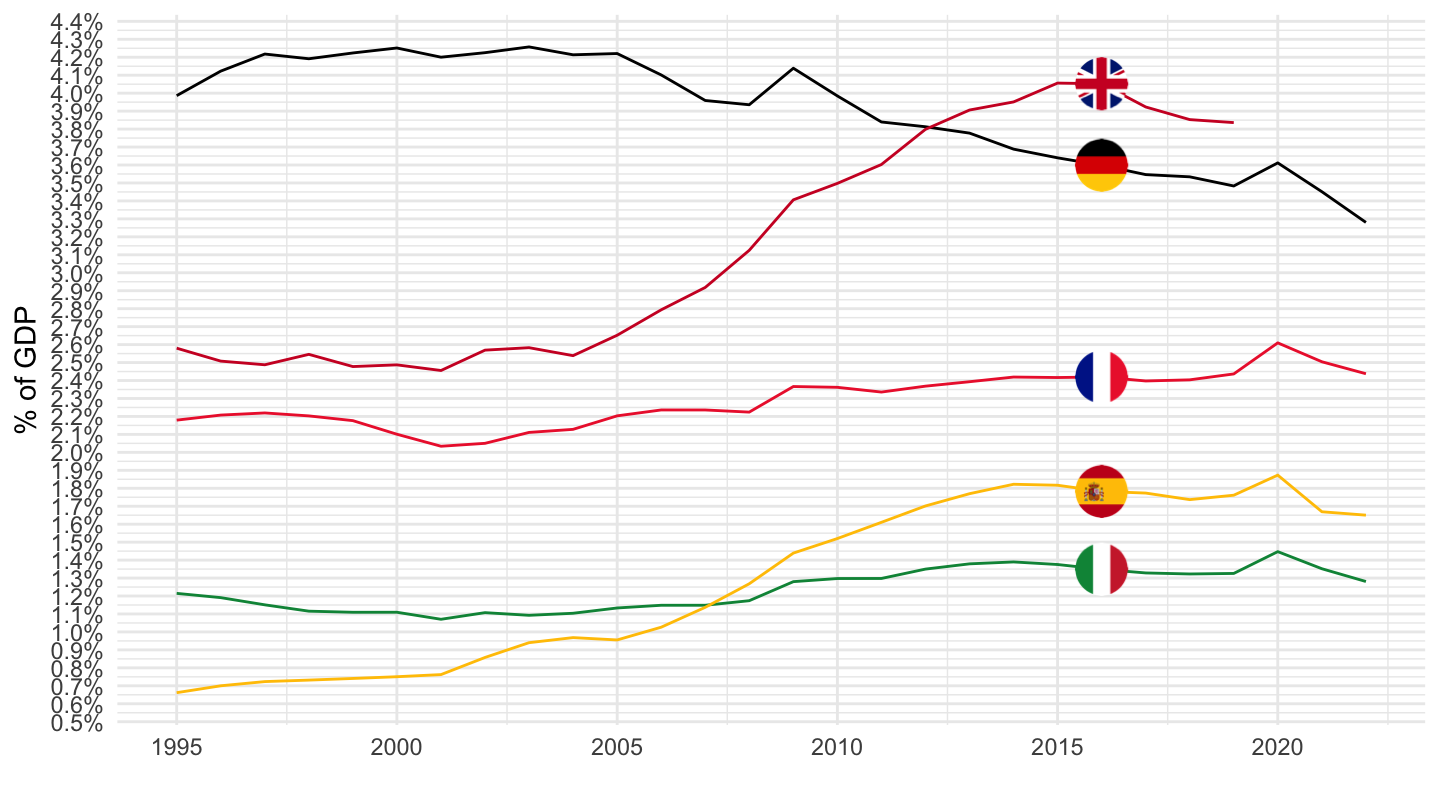
CP042
Nominal
Code
nama_10_co3_p3 %>%
  filter(unit == "CP_MEUR",
         geo %in% c("FR", "UK", "IT", "ES", "DE"),
         coicop == "CP042") %>%
  left_join(nama_10_gdp %>%
              filter(na_item == "B1GQ",
                     unit == "CP_MEUR") %>%
              select(geo, time, gdp = values),
            by = c("geo", "time")) %>%
  left_join(geo, by = "geo") %>%
  year_to_date %>%
  filter(date >= as.Date("1995-01-01")) %>%
  left_join(colors, by = c("Geo" = "country")) %>%
  mutate(values = values/gdp) %>%
  ggplot + geom_line(aes(x = date, y = values, color = color)) +
  theme_minimal()  + add_5flags +
  scale_color_identity() + xlab("") + ylab("% of GDP") +
  scale_x_date(breaks = as.Date(paste0(seq(1960, 2100, 5), "-01-01")),
               labels = date_format("%Y")) +
  theme(legend.position = c(0.2, 0.85),
        legend.title = element_blank()) +
  scale_y_continuous(breaks = 0.01*seq(0, 200, 1),
                     labels = scales::percent_format(accuracy = 1))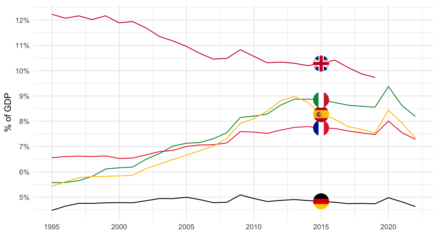
CP091
Real
Code
nama_10_co3_p3 %>%
  filter(unit == "CLV10_MEUR",
         geo %in% c("FR", "NL", "IT", "ES", "DE"),
         coicop == "CP091") %>%
  left_join(nama_10_gdp %>%
              filter(na_item == "B1GQ",
                     unit == "CLV10_MEUR") %>%
              select(geo, time, gdp = values),
            by = c("geo", "time")) %>%
  left_join(geo, by = "geo") %>%
  year_to_date %>%
  filter(date >= as.Date("1995-01-01")) %>%
  left_join(colors, by = c("Geo" = "country")) %>%
  mutate(values = values/gdp) %>%
  ggplot + geom_line(aes(x = date, y = values, color = color)) +
  theme_minimal()  + add_5flags +
  scale_color_identity() + xlab("") + ylab("% of GDP") +
  scale_x_date(breaks = as.Date(paste0(seq(1960, 2100, 5), "-01-01")),
               labels = date_format("%Y")) +
  theme(legend.position = c(0.2, 0.85),
        legend.title = element_blank()) +
  scale_y_continuous(breaks = 0.01*seq(0, 200, .1),
                     labels = scales::percent_format(accuracy = .1))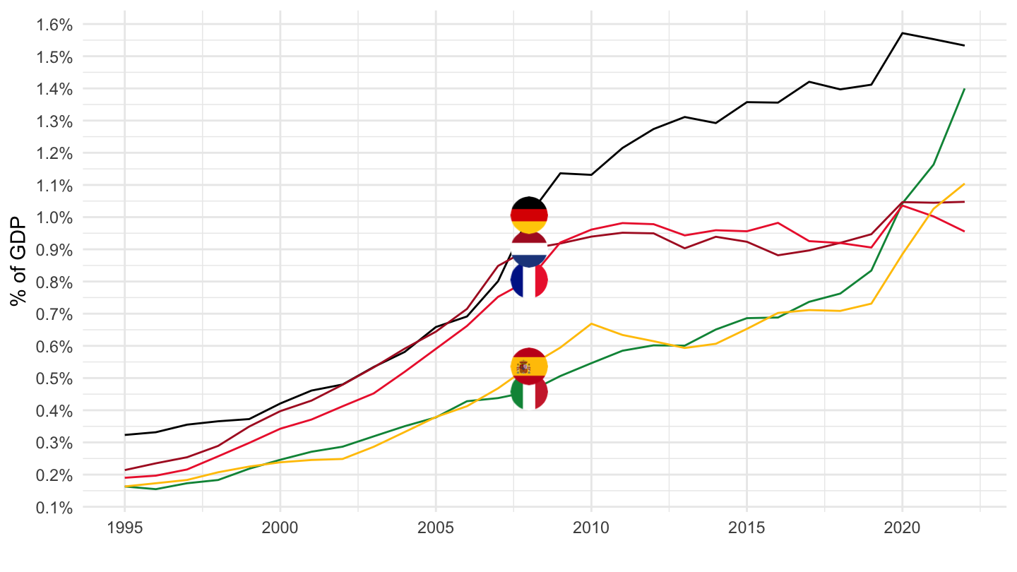
Nominal
Code
nama_10_co3_p3 %>%
  filter(unit == "CP_MEUR",
         geo %in% c("FR", "UK", "IT", "ES", "DE"),
         coicop == "CP091") %>%
  left_join(nama_10_gdp %>%
              filter(na_item == "B1GQ",
                     unit == "CP_MEUR") %>%
              select(geo, time, gdp = values),
            by = c("geo", "time")) %>%
  left_join(geo, by = "geo") %>%
  year_to_date %>%
  filter(date >= as.Date("1995-01-01")) %>%
  left_join(colors, by = c("Geo" = "country")) %>%
  mutate(values = values/gdp) %>%
  ggplot + geom_line(aes(x = date, y = values, color = color)) +
  theme_minimal()  + add_5flags +
  scale_color_identity() + xlab("") + ylab("% of GDP") +
  scale_x_date(breaks = as.Date(paste0(seq(1960, 2100, 5), "-01-01")),
               labels = date_format("%Y")) +
  theme(legend.position = c(0.2, 0.85),
        legend.title = element_blank()) +
  scale_y_continuous(breaks = 0.01*seq(0, 200, .1),
                     labels = scales::percent_format(accuracy = .1))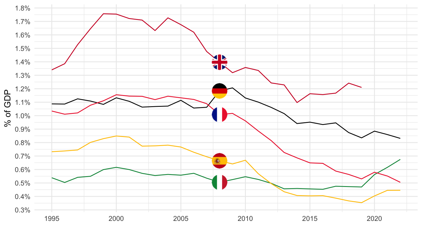
CP081 - Postal Services
Real
Code
nama_10_co3_p3 %>%
  filter(unit == "CLV10_MEUR",
         geo %in% c("FR", "UK", "IT", "ES", "DE"),
         coicop == "CP081") %>%
  left_join(nama_10_gdp %>%
              filter(na_item == "B1GQ",
                     unit == "CLV10_MEUR") %>%
              select(geo, time, gdp = values),
            by = c("geo", "time")) %>%
  left_join(geo, by = "geo") %>%
  year_to_date %>%
  filter(date >= as.Date("1995-01-01")) %>%
  left_join(colors, by = c("Geo" = "country")) %>%
  mutate(values = values/gdp) %>%
  ggplot + geom_line(aes(x = date, y = values, color = color)) +
  theme_minimal()  + add_5flags +
  scale_color_identity() + xlab("") + ylab("% of GDP") +
  scale_x_date(breaks = as.Date(paste0(seq(1960, 2100, 5), "-01-01")),
               labels = date_format("%Y")) +
  theme(legend.position = c(0.2, 0.85),
        legend.title = element_blank()) +
  scale_y_continuous(breaks = 0.01*seq(0, 200, .05),
                     labels = scales::percent_format(accuracy = .01))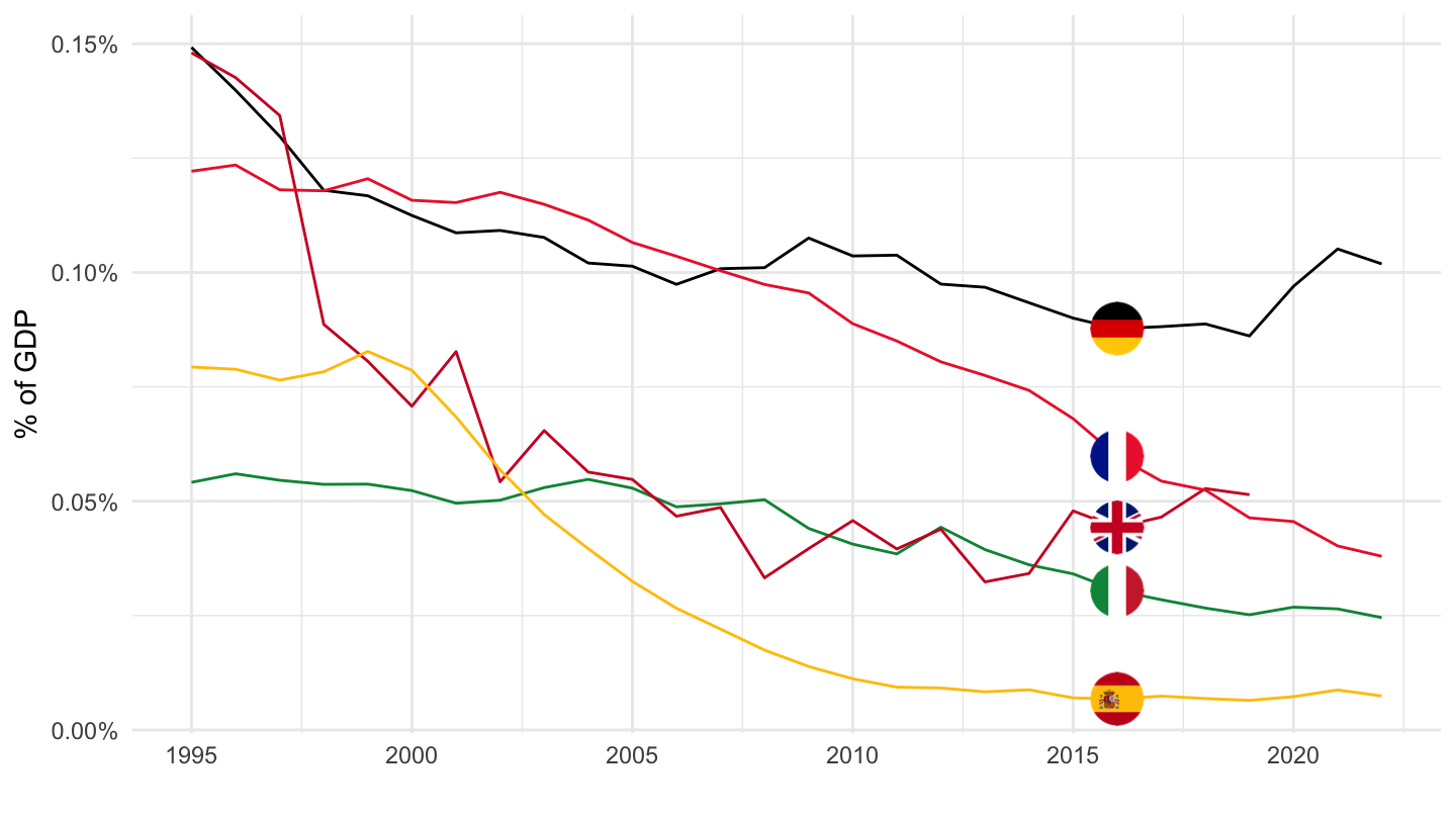
Nominal
Code
nama_10_co3_p3 %>%
  filter(unit == "CP_MEUR",
         geo %in% c("FR", "UK", "IT", "ES", "DE"),
         coicop == "CP081") %>%
  left_join(nama_10_gdp %>%
              filter(na_item == "B1GQ",
                     unit == "CP_MEUR") %>%
              select(geo, time, gdp = values),
            by = c("geo", "time")) %>%
  left_join(geo, by = "geo") %>%
  year_to_date %>%
  filter(date >= as.Date("1995-01-01")) %>%
  left_join(colors, by = c("Geo" = "country")) %>%
  mutate(values = values/gdp) %>%
  ggplot + geom_line(aes(x = date, y = values, color = color)) +
  theme_minimal()  + add_5flags +
  scale_color_identity() + xlab("") + ylab("% of GDP") +
  scale_x_date(breaks = as.Date(paste0(seq(1960, 2100, 5), "-01-01")),
               labels = date_format("%Y")) +
  theme(legend.position = c(0.2, 0.85),
        legend.title = element_blank()) +
  scale_y_continuous(breaks = 0.01*seq(0, 200, .05),
                     labels = scales::percent_format(accuracy = .01))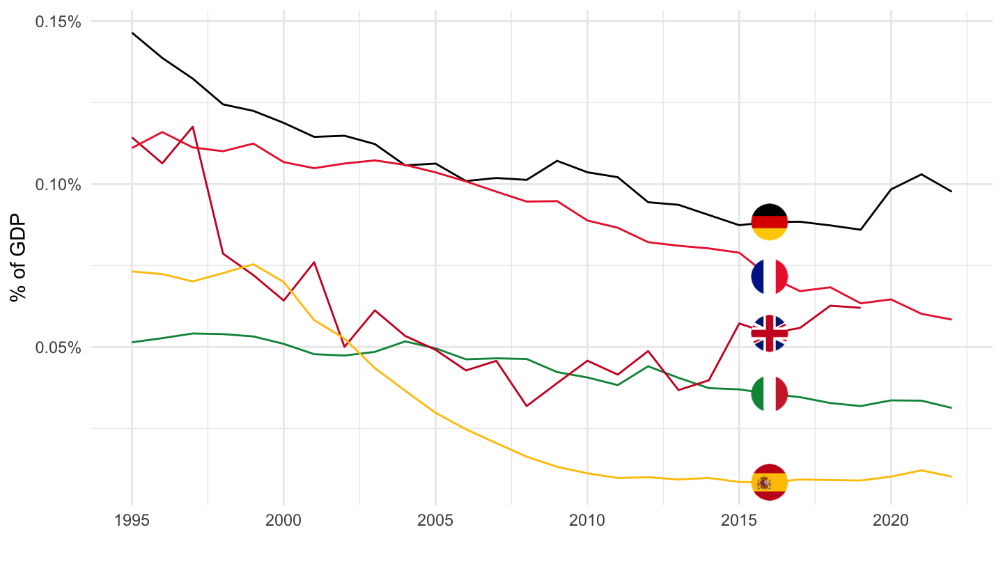
CP082 - Telephone and telefax equipment
Real
Code
nama_10_co3_p3 %>%
  filter(unit == "CLV10_MEUR",
         geo %in% c("FR", "NL", "IT", "ES", "DE"),
         coicop == "CP082") %>%
  left_join(nama_10_gdp %>%
              filter(na_item == "B1GQ",
                     unit == "CLV10_MEUR") %>%
              select(geo, time, gdp = values),
            by = c("geo", "time")) %>%
  left_join(geo, by = "geo") %>%
  year_to_date %>%
  filter(date >= as.Date("1995-01-01")) %>%
  left_join(colors, by = c("Geo" = "country")) %>%
  mutate(values = values/gdp) %>%
  ggplot + geom_line(aes(x = date, y = values, color = color)) +
  theme_minimal()  + add_5flags +
  scale_color_identity() + xlab("") + ylab("% of GDP") +
  scale_x_date(breaks = as.Date(paste0(seq(1960, 2100, 5), "-01-01")),
               labels = date_format("%Y")) +
  theme(legend.position = c(0.2, 0.85),
        legend.title = element_blank()) +
  scale_y_continuous(breaks = 0.01*seq(0, 200, .1),
                     labels = scales::percent_format(accuracy = .1))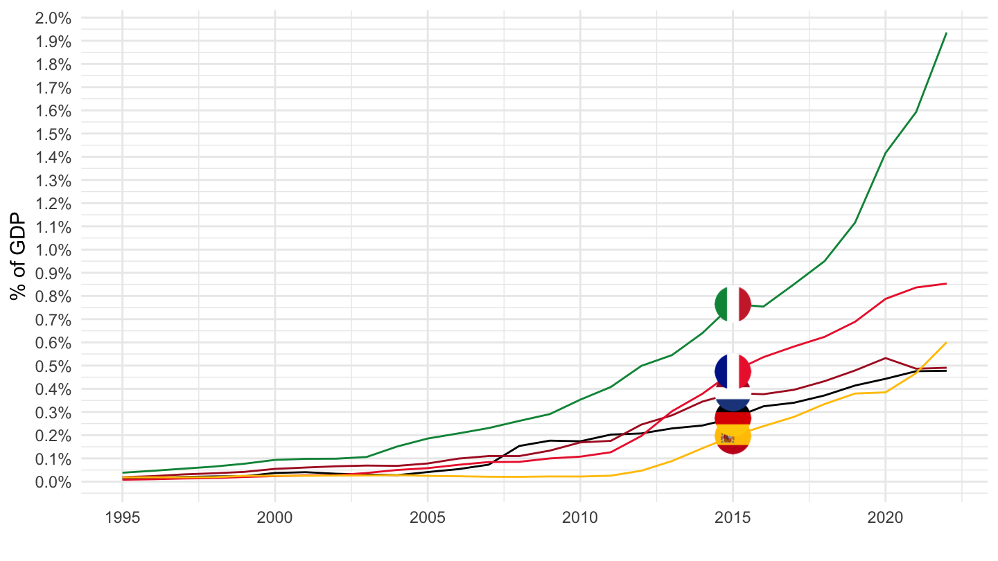
Nominal
Code
nama_10_co3_p3 %>%
  filter(unit == "CP_MEUR",
         geo %in% c("FR", "UK", "IT", "ES", "DE"),
         coicop == "CP082") %>%
  left_join(nama_10_gdp %>%
              filter(na_item == "B1GQ",
                     unit == "CP_MEUR") %>%
              select(geo, time, gdp = values),
            by = c("geo", "time")) %>%
  left_join(geo, by = "geo") %>%
  year_to_date %>%
  filter(date >= as.Date("1995-01-01")) %>%
  left_join(colors, by = c("Geo" = "country")) %>%
  mutate(values = values/gdp) %>%
  ggplot + geom_line(aes(x = date, y = values, color = color)) +
  theme_minimal()  + add_5flags +
  scale_color_identity() + xlab("") + ylab("% of GDP") +
  scale_x_date(breaks = as.Date(paste0(seq(1960, 2100, 5), "-01-01")),
               labels = date_format("%Y")) +
  theme(legend.position = c(0.2, 0.85),
        legend.title = element_blank()) +
  scale_y_continuous(breaks = 0.01*seq(0, 200, .1),
                     labels = scales::percent_format(accuracy = .1))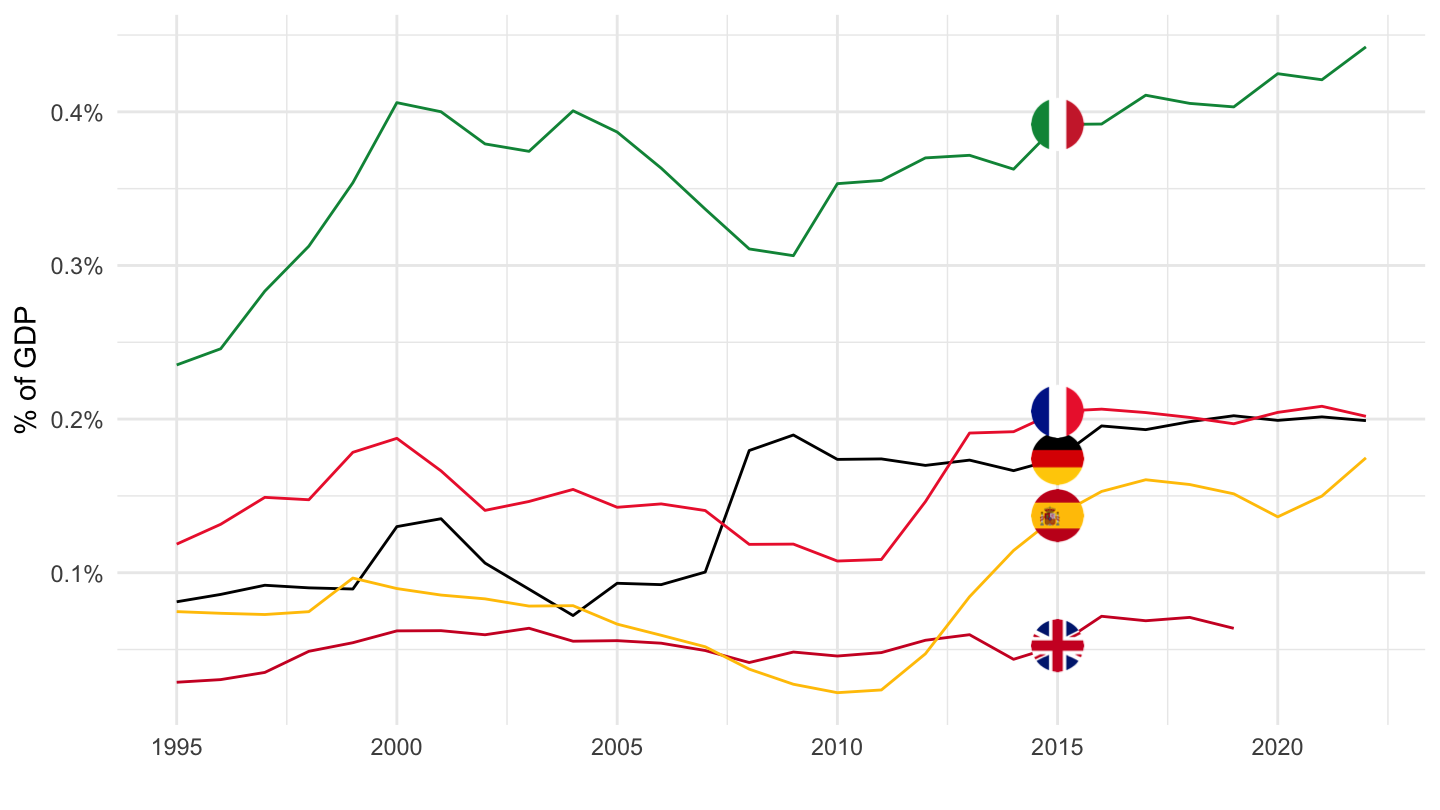
CP071- Cars
1995-
Code
nama_10_co3_p3 %>%
  filter(unit == "CP_MEUR",
         geo %in% c("FR", "UK", "IT", "ES", "DE"),
         coicop == "CP071") %>%
  left_join(nama_10_gdp %>%
              filter(na_item == "B1GQ",
                     unit == "CP_MEUR") %>%
              select(geo, time, gdp = values),
            by = c("geo", "time")) %>%
  left_join(geo, by = "geo") %>%
  year_to_date %>%
  filter(date >= as.Date("1995-01-01")) %>%
  left_join(colors, by = c("Geo" = "country")) %>%
  mutate(values = values/gdp) %>%
  ggplot + geom_line(aes(x = date, y = values, color = color)) +
  theme_minimal()  + add_5flags +
  scale_color_identity() + xlab("") + ylab("% of GDP") +
  scale_x_date(breaks = as.Date(paste0(seq(1960, 2100, 5), "-01-01")),
               labels = date_format("%Y")) +
  theme(legend.position = c(0.2, 0.85),
        legend.title = element_blank()) +
  scale_y_continuous(breaks = 0.01*seq(0, 200, .1),
                     labels = scales::percent_format(accuracy = .1))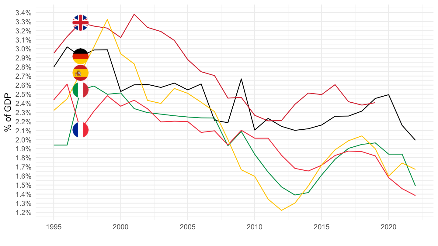
CP083 - Telephone and telefax services
Real (% of GDP)
1995-
Code
nama_10_co3_p3 %>%
  filter(unit == "CLV10_MEUR",
         geo %in% c("FR", "NL", "IT", "ES", "DE"),
         coicop == "CP083") %>%
  left_join(nama_10_gdp %>%
              filter(na_item == "B1GQ",
                     unit == "CLV10_MEUR") %>%
              select(geo, time, gdp = values),
            by = c("geo", "time")) %>%
  left_join(geo, by = "geo") %>%
  year_to_date %>%
  filter(date >= as.Date("1995-01-01")) %>%
  left_join(colors, by = c("Geo" = "country")) %>%
  mutate(values = values/gdp) %>%
  ggplot + geom_line(aes(x = date, y = values, color = color)) +
  theme_minimal()  + add_5flags +
  scale_color_identity() + xlab("") + ylab("% of GDP") +
  scale_x_date(breaks = as.Date(paste0(seq(1960, 2100, 5), "-01-01")),
               labels = date_format("%Y")) +
  theme(legend.position = c(0.2, 0.85),
        legend.title = element_blank()) +
  scale_y_continuous(breaks = 0.01*seq(0, 200, .1),
                     labels = scales::percent_format(accuracy = .1))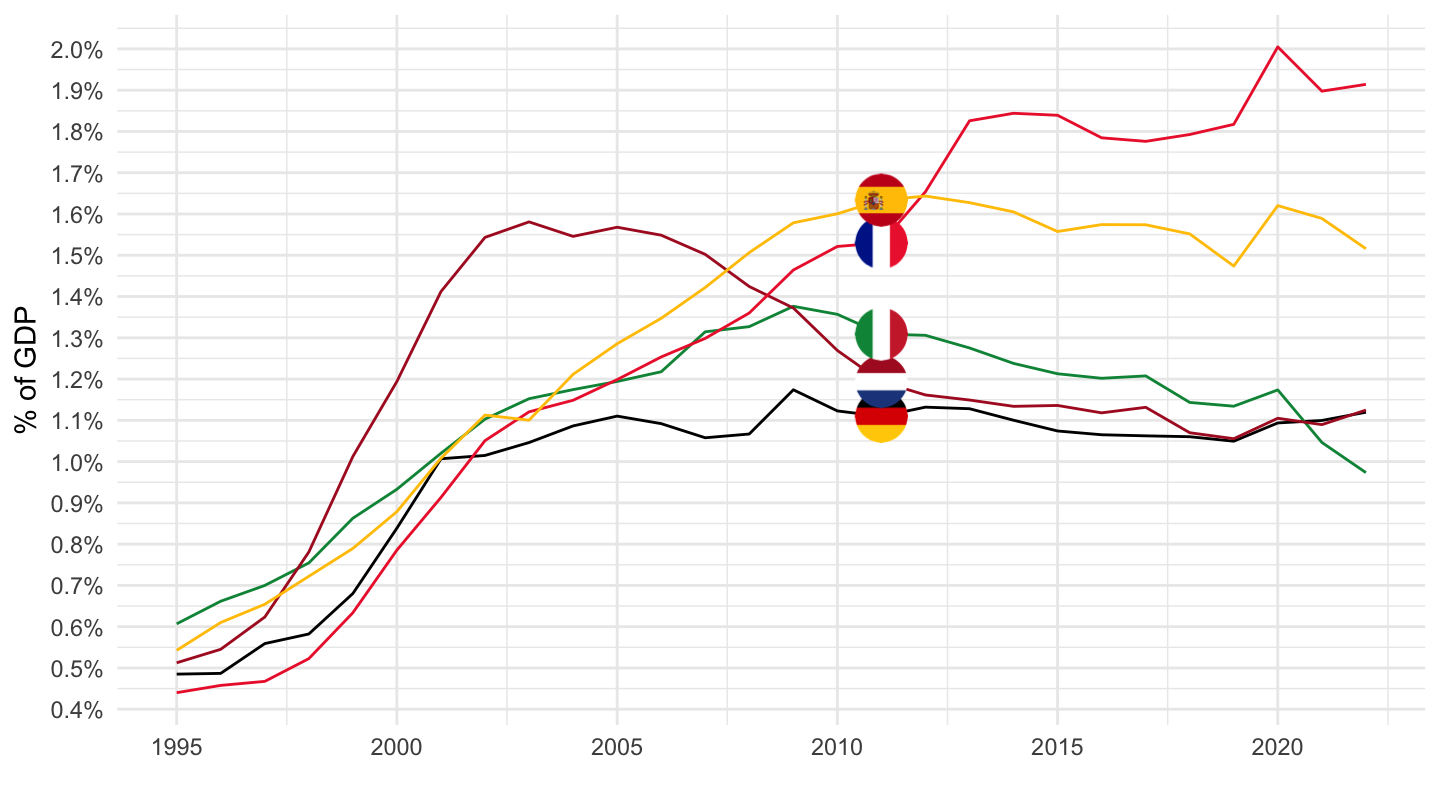
2005-2015
Code
nama_10_co3_p3 %>%
  filter(unit == "CLV10_MEUR",
         geo %in% c("FR", "NL", "IT", "ES", "DE"),
         coicop == "CP083") %>%
  left_join(nama_10_gdp %>%
              filter(na_item == "B1GQ",
                     unit == "CLV10_MEUR") %>%
              select(geo, time, gdp = values),
            by = c("geo", "time")) %>%
  left_join(geo, by = "geo") %>%
  year_to_date %>%
  filter(date >= as.Date("2005-01-01"),
         date <= as.Date("2016-01-01")) %>%
  left_join(colors, by = c("Geo" = "country")) %>%
  mutate(values = values/gdp) %>%
  ggplot + geom_line(aes(x = date, y = values, color = color)) +
  theme_minimal()  + add_5flags +
  scale_color_identity() + xlab("") + ylab("% of GDP") +
  scale_x_date(breaks = as.Date(paste0(seq(1960, 2100, 1), "-01-01")),
               labels = date_format("%Y")) +
  theme(legend.position = c(0.2, 0.85),
        legend.title = element_blank()) +
  scale_y_continuous(breaks = 0.01*seq(0, 200, .1),
                     labels = scales::percent_format(accuracy = .1))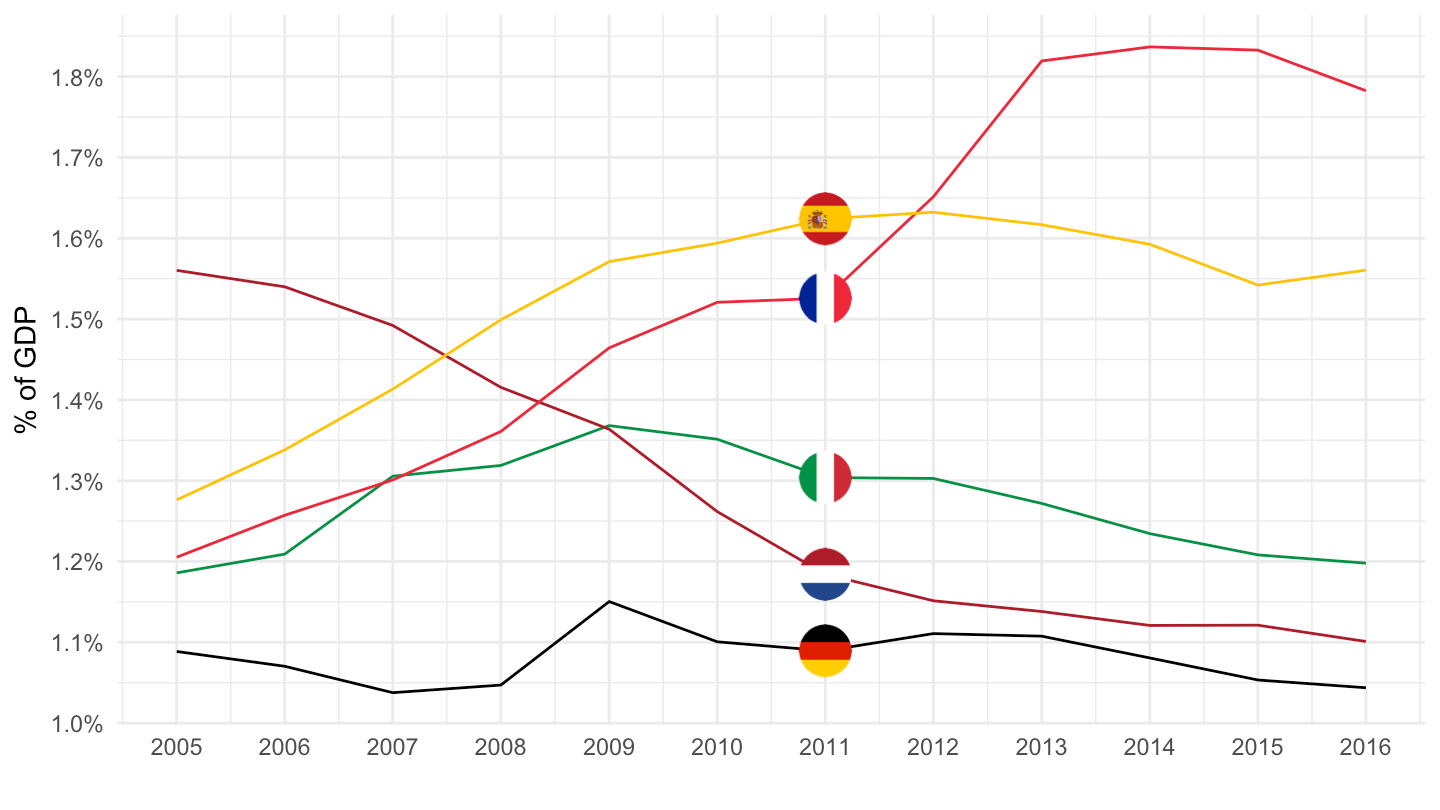
2010-2014
Code
nama_10_co3_p3 %>%
  filter(unit == "CLV10_MEUR",
         geo %in% c("FR", "NL", "IT", "ES", "DE"),
         coicop == "CP083") %>%
  left_join(nama_10_gdp %>%
              filter(na_item == "B1GQ",
                     unit == "CLV10_MEUR") %>%
              select(geo, time, gdp = values),
            by = c("geo", "time")) %>%
  left_join(geo, by = "geo") %>%
  year_to_date %>%
  filter(date >= as.Date("2010-01-01"),
         date <= as.Date("2014-12-01")) %>%
  left_join(colors, by = c("Geo" = "country")) %>%
  mutate(values = values/gdp) %>%
  ggplot + geom_line(aes(x = date, y = values, color = color)) +
  theme_minimal()  + add_5flags +
  scale_color_identity() + xlab("") + ylab("% of GDP") +
  scale_x_date(breaks = as.Date(paste0(seq(1960, 2100, 1), "-01-01")),
               labels = date_format("%Y")) +
  theme(legend.position = c(0.2, 0.85),
        legend.title = element_blank()) +
  scale_y_continuous(breaks = 0.01*seq(0, 200, .05),
                     labels = scales::percent_format(accuracy = .01))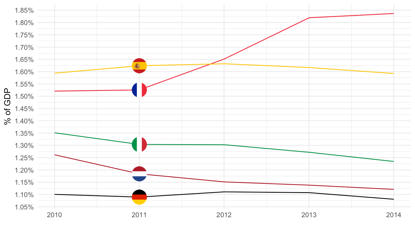
2011-2013
Code
nama_10_co3_p3 %>%
  filter(unit == "CLV10_MEUR",
         geo %in% c("FR", "NL", "IT", "ES", "DE"),
         coicop == "CP083") %>%
  left_join(nama_10_gdp %>%
              filter(na_item == "B1GQ",
                     unit == "CLV10_MEUR") %>%
              select(geo, time, gdp = values),
            by = c("geo", "time")) %>%
  left_join(geo, by = "geo") %>%
  year_to_date %>%
  filter(date >= as.Date("2011-01-01"),
         date <= as.Date("2013-12-01")) %>%
  left_join(colors, by = c("Geo" = "country")) %>%
  mutate(values = values/gdp) %>%
  ggplot + geom_line(aes(x = date, y = values, color = color)) +
  theme_minimal()  + add_5flags +
  scale_color_identity() + xlab("") + ylab("% of GDP") +
  scale_x_date(breaks = as.Date(paste0(seq(1960, 2100, 1), "-01-01")),
               labels = date_format("%Y")) +
  theme(legend.position = c(0.2, 0.85),
        legend.title = element_blank()) +
  scale_y_continuous(breaks = 0.01*seq(0, 200, .05),
                     labels = scales::percent_format(accuracy = .01))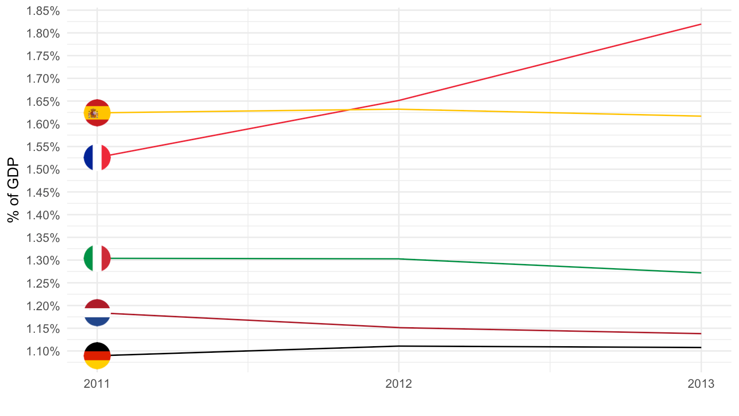
Real (% of Consumption)
Code
nama_10_co3_p3 %>%
  filter(unit == "CLV10_MEUR",
         geo %in% c("FR", "UK", "IT", "ES", "DE"),
         coicop == "CP083") %>%
  left_join(nama_10_gdp %>%
              filter(na_item == "P31_S14",
                     unit == "CLV10_MEUR") %>%
              select(geo, time, cons = values),
            by = c("geo", "time")) %>%
  left_join(geo, by = "geo") %>%
  year_to_date %>%
  filter(date >= as.Date("1995-01-01")) %>%
  left_join(colors, by = c("Geo" = "country")) %>%
  mutate(values = values/cons) %>%
  ggplot + geom_line(aes(x = date, y = values, color = color)) +
  theme_minimal()  + add_5flags +
  scale_color_identity() + xlab("") + ylab("Telephone and telefax services (% of Cons.)") +
  scale_x_date(breaks = as.Date(paste0(seq(1960, 2100, 5), "-01-01")),
               labels = date_format("%Y")) +
  theme(legend.position = c(0.2, 0.85),
        legend.title = element_blank()) +
  scale_y_continuous(breaks = 0.01*seq(0, 200, .2),
                     labels = scales::percent_format(accuracy = .1))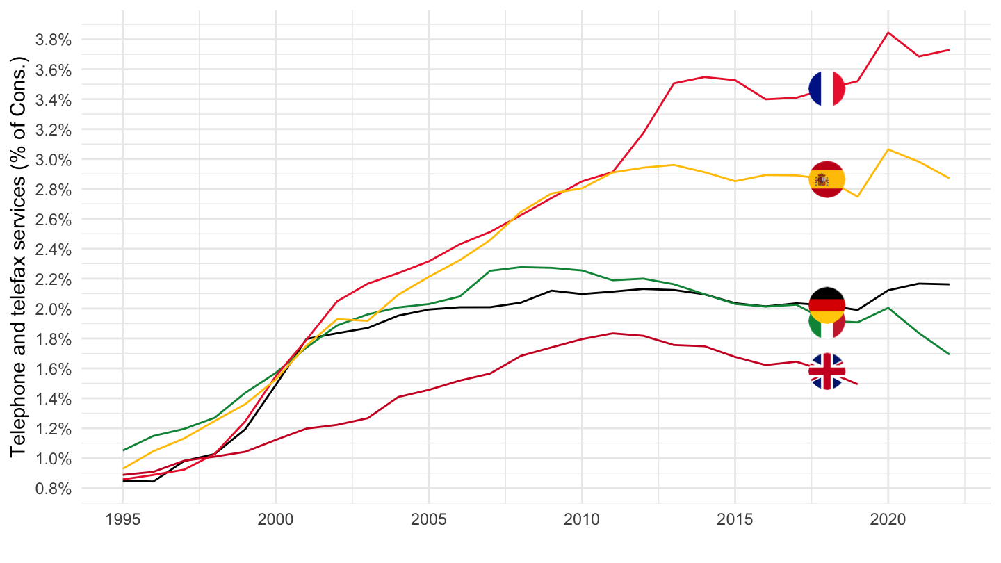
Nominal
1995-
Code
nama_10_co3_p3 %>%
  filter(unit == "CP_MEUR",
         geo %in% c("FR", "UK", "IT", "ES", "DE"),
         coicop == "CP083") %>%
  left_join(nama_10_gdp %>%
              filter(na_item == "B1GQ",
                     unit == "CP_MEUR") %>%
              select(geo, time, gdp = values),
            by = c("geo", "time")) %>%
  left_join(geo, by = "geo") %>%
  year_to_date %>%
  filter(date >= as.Date("1995-01-01")) %>%
  left_join(colors, by = c("Geo" = "country")) %>%
  mutate(values = values/gdp) %>%
  ggplot + geom_line(aes(x = date, y = values, color = color)) +
  theme_minimal()  + add_5flags +
  scale_color_identity() + xlab("") + ylab("% of GDP") +
  scale_x_date(breaks = as.Date(paste0(seq(1960, 2100, 5), "-01-01")),
               labels = date_format("%Y")) +
  theme(legend.position = c(0.2, 0.85),
        legend.title = element_blank()) +
  scale_y_continuous(breaks = 0.01*seq(0, 200, .1),
                     labels = scales::percent_format(accuracy = .1))
2005-2015
Code
nama_10_co3_p3 %>%
  filter(unit == "CP_MEUR",
         geo %in% c("FR", "UK", "IT", "ES", "DE"),
         coicop == "CP083") %>%
  left_join(nama_10_gdp %>%
              filter(na_item == "B1GQ",
                     unit == "CP_MEUR") %>%
              select(geo, time, gdp = values),
            by = c("geo", "time")) %>%
  left_join(geo, by = "geo") %>%
  year_to_date %>%
  filter(date >= as.Date("2005-01-01"),
         date <= as.Date("2016-01-01")) %>%
  left_join(colors, by = c("Geo" = "country")) %>%
  mutate(values = values/gdp) %>%
  ggplot + geom_line(aes(x = date, y = values, color = color)) +
  theme_minimal()  + add_5flags +
  scale_color_identity() + xlab("") + ylab("% of GDP") +
  scale_x_date(breaks = as.Date(paste0(seq(1960, 2100, 1), "-01-01")),
               labels = date_format("%Y")) +
  theme(legend.position = c(0.2, 0.85),
        legend.title = element_blank()) +
  scale_y_continuous(breaks = 0.01*seq(0, 200, .1),
                     labels = scales::percent_format(accuracy = .1))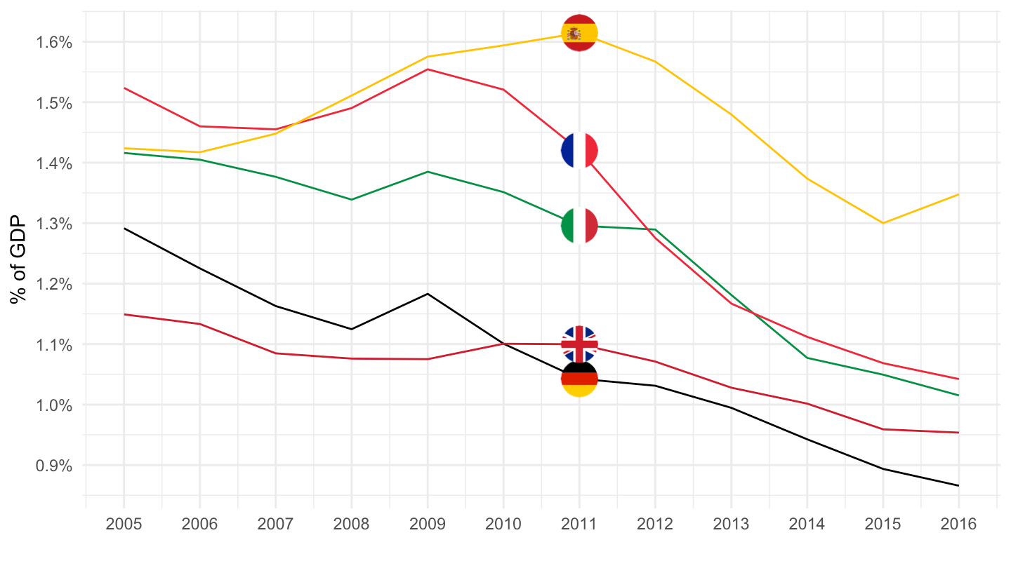
2011-2013
Code
nama_10_co3_p3 %>%
  filter(unit == "CP_MEUR",
         geo %in% c("FR", "UK", "IT", "ES", "DE"),
         coicop == "CP083") %>%
  left_join(nama_10_gdp %>%
              filter(na_item == "B1GQ",
                     unit == "CP_MEUR") %>%
              select(geo, time, gdp = values),
            by = c("geo", "time")) %>%
  left_join(geo, by = "geo") %>%
  year_to_date %>%
  filter(date >= as.Date("2011-01-01"),
         date <= as.Date("2013-01-01")) %>%
  left_join(colors, by = c("Geo" = "country")) %>%
  mutate(values = values/gdp) %>%
  ggplot + geom_line(aes(x = date, y = values, color = color)) +
  theme_minimal()  + add_5flags +
  scale_color_identity() + xlab("") + ylab("% of GDP") +
  scale_x_date(breaks = as.Date(paste0(seq(1960, 2100, 1), "-01-01")),
               labels = date_format("%Y")) +
  theme(legend.position = c(0.2, 0.85),
        legend.title = element_blank()) +
  scale_y_continuous(breaks = 0.01*seq(0, 200, .1),
                     labels = scales::percent_format(accuracy = .1))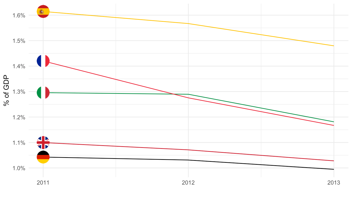
CP08 - Communications
Real
Code
nama_10_co3_p3 %>%
  filter(unit == "CLV10_MEUR",
         geo %in% c("FR", "UK", "IT", "ES", "DE"),
         coicop == "CP08") %>%
  left_join(nama_10_gdp %>%
              filter(na_item == "B1GQ",
                     unit == "CLV10_MEUR") %>%
              select(geo, time, gdp = values),
            by = c("geo", "time")) %>%
  left_join(geo, by = "geo") %>%
  year_to_date %>%
  filter(date >= as.Date("1995-01-01")) %>%
  left_join(colors, by = c("Geo" = "country")) %>%
  mutate(values = values/gdp) %>%
  ggplot + geom_line(aes(x = date, y = values, color = color)) +
  theme_minimal()  + add_5flags +
  scale_color_identity() + xlab("") + ylab("% of GDP") +
  scale_x_date(breaks = as.Date(paste0(seq(1960, 2100, 5), "-01-01")),
               labels = date_format("%Y")) +
  theme(legend.position = c(0.2, 0.85),
        legend.title = element_blank()) +
  scale_y_continuous(breaks = 0.01*seq(0, 200, .1),
                     labels = scales::percent_format(accuracy = .1))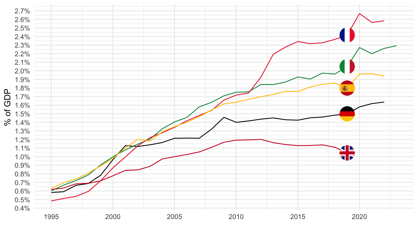
Nominal
Code
nama_10_co3_p3 %>%
  filter(unit == "CP_MEUR",
         geo %in% c("FR", "UK", "IT", "ES", "DE"),
         coicop == "CP08") %>%
  left_join(nama_10_gdp %>%
              filter(na_item == "B1GQ",
                     unit == "CP_MEUR") %>%
              select(geo, time, gdp = values),
            by = c("geo", "time")) %>%
  left_join(geo, by = "geo") %>%
  year_to_date %>%
  filter(date >= as.Date("1995-01-01")) %>%
  left_join(colors, by = c("Geo" = "country")) %>%
  mutate(values = values/gdp) %>%
  ggplot + geom_line(aes(x = date, y = values, color = color)) +
  theme_minimal()  + add_5flags +
  scale_color_identity() + xlab("") + ylab("% of GDP") +
  scale_x_date(breaks = as.Date(paste0(seq(1960, 2100, 5), "-01-01")),
               labels = date_format("%Y")) +
  theme(legend.position = c(0.2, 0.85),
        legend.title = element_blank()) +
  scale_y_continuous(breaks = 0.01*seq(0, 200, .1),
                     labels = scales::percent_format(accuracy = .1))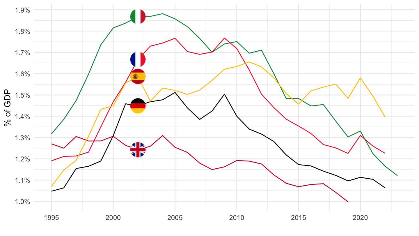
CP09 - Recreation and Culture
Real
Code
nama_10_co3_p3 %>%
  filter(unit == "CLV10_MEUR",
         geo %in% c("FR", "UK", "IT", "ES", "DE"),
         coicop == "CP09") %>%
  left_join(nama_10_gdp %>%
              filter(na_item == "B1GQ",
                     unit == "CLV10_MEUR") %>%
              select(geo, time, gdp = values),
            by = c("geo", "time")) %>%
  left_join(geo, by = "geo") %>%
  year_to_date %>%
  filter(date >= as.Date("1995-01-01")) %>%
  left_join(colors, by = c("Geo" = "country")) %>%
  mutate(values = values/gdp) %>%
  ggplot + geom_line(aes(x = date, y = values, color = color)) +
  theme_minimal()  + add_5flags +
  scale_color_identity() + xlab("") + ylab("% of GDP") +
  scale_x_date(breaks = as.Date(paste0(seq(1960, 2100, 5), "-01-01")),
               labels = date_format("%Y")) +
  theme(legend.position = c(0.2, 0.85),
        legend.title = element_blank()) +
  scale_y_continuous(breaks = 0.01*seq(0, 200, .1),
                     labels = scales::percent_format(accuracy = .1))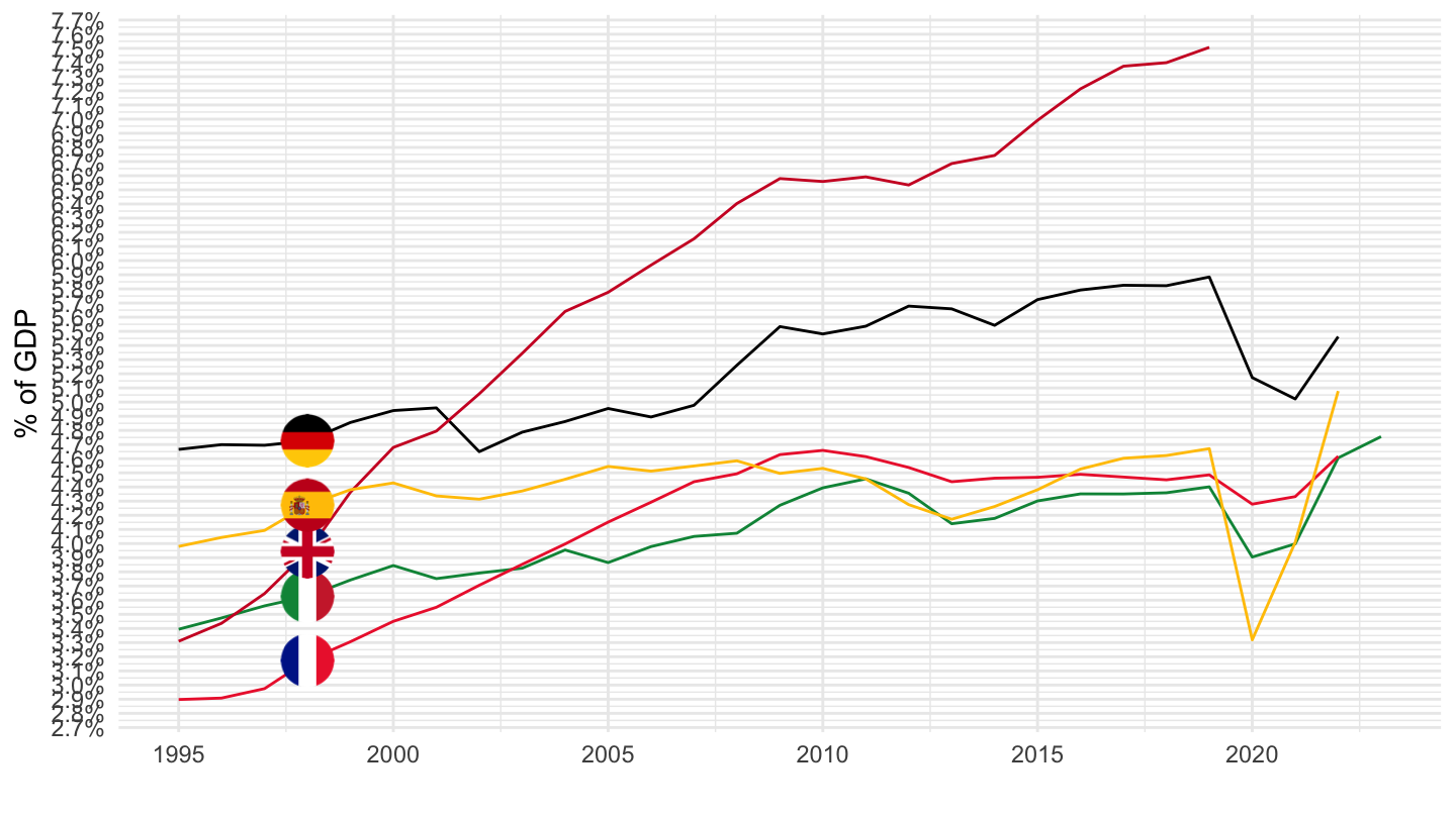
Nominal
Code
nama_10_co3_p3 %>%
  filter(unit == "CP_MEUR",
         geo %in% c("FR", "UK", "IT", "ES", "DE"),
         coicop == "CP09") %>%
  left_join(nama_10_gdp %>%
              filter(na_item == "B1GQ",
                     unit == "CP_MEUR") %>%
              select(geo, time, gdp = values),
            by = c("geo", "time")) %>%
  left_join(geo, by = "geo") %>%
  year_to_date %>%
  filter(date >= as.Date("1995-01-01")) %>%
  left_join(colors, by = c("Geo" = "country")) %>%
  mutate(values = values/gdp) %>%
  ggplot + geom_line(aes(x = date, y = values, color = color)) +
  theme_minimal()  + add_5flags +
  scale_color_identity() + xlab("") + ylab("% of GDP") +
  scale_x_date(breaks = as.Date(paste0(seq(1960, 2100, 5), "-01-01")),
               labels = date_format("%Y")) +
  theme(legend.position = c(0.2, 0.85),
        legend.title = element_blank()) +
  scale_y_continuous(breaks = 0.01*seq(0, 200, .1),
                     labels = scales::percent_format(accuracy = .1))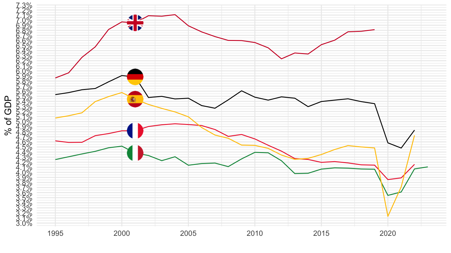
CP126 - Financial Services
Real
Code
nama_10_co3_p3 %>%
  filter(unit == "CLV10_MEUR",
         geo %in% c("FR", "UK", "IT", "ES", "DE"),
         coicop == "CP126") %>%
  left_join(nama_10_gdp %>%
              filter(na_item == "B1GQ",
                     unit == "CLV10_MEUR") %>%
              select(geo, time, gdp = values),
            by = c("geo", "time")) %>%
  left_join(geo, by = "geo") %>%
  year_to_date %>%
  filter(date >= as.Date("1995-01-01")) %>%
  left_join(colors, by = c("Geo" = "country")) %>%
  mutate(values = values/gdp) %>%
  ggplot + geom_line(aes(x = date, y = values, color = color)) +
  theme_minimal()  + add_5flags +
  scale_color_identity() + xlab("") + ylab("% of GDP") +
  scale_x_date(breaks = as.Date(paste0(seq(1960, 2100, 5), "-01-01")),
               labels = date_format("%Y")) +
  theme(legend.position = c(0.2, 0.85),
        legend.title = element_blank()) +
  scale_y_continuous(breaks = 0.01*seq(0, 200, .1),
                     labels = scales::percent_format(accuracy = .1))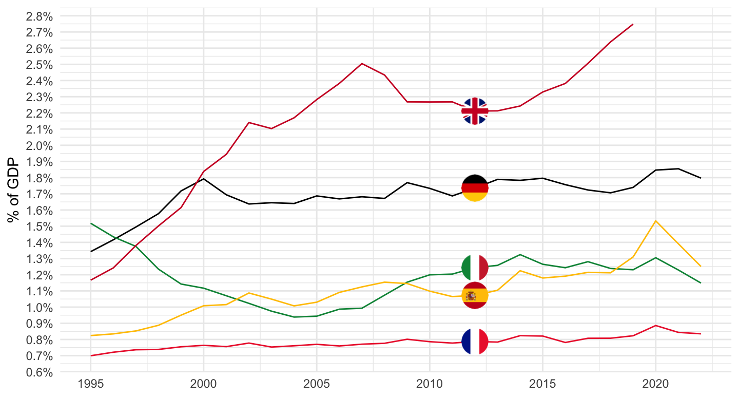
Nominal
Code
nama_10_co3_p3 %>%
  filter(unit == "CP_MEUR",
         geo %in% c("FR", "UK", "IT", "ES", "DE"),
         coicop == "CP126") %>%
  left_join(nama_10_gdp %>%
              filter(na_item == "B1GQ",
                     unit == "CP_MEUR") %>%
              select(geo, time, gdp = values),
            by = c("geo", "time")) %>%
  left_join(geo, by = "geo") %>%
  year_to_date %>%
  filter(date >= as.Date("1995-01-01")) %>%
  left_join(colors, by = c("Geo" = "country")) %>%
  mutate(values = values/gdp) %>%
  ggplot + geom_line(aes(x = date, y = values, color = color)) +
  theme_minimal()  + add_5flags +
  scale_color_identity() + xlab("") + ylab("% of GDP") +
  scale_x_date(breaks = as.Date(paste0(seq(1960, 2100, 5), "-01-01")),
               labels = date_format("%Y")) +
  theme(legend.position = c(0.2, 0.85),
        legend.title = element_blank()) +
  scale_y_continuous(breaks = 0.01*seq(0, 200, .1),
                     labels = scales::percent_format(accuracy = .1))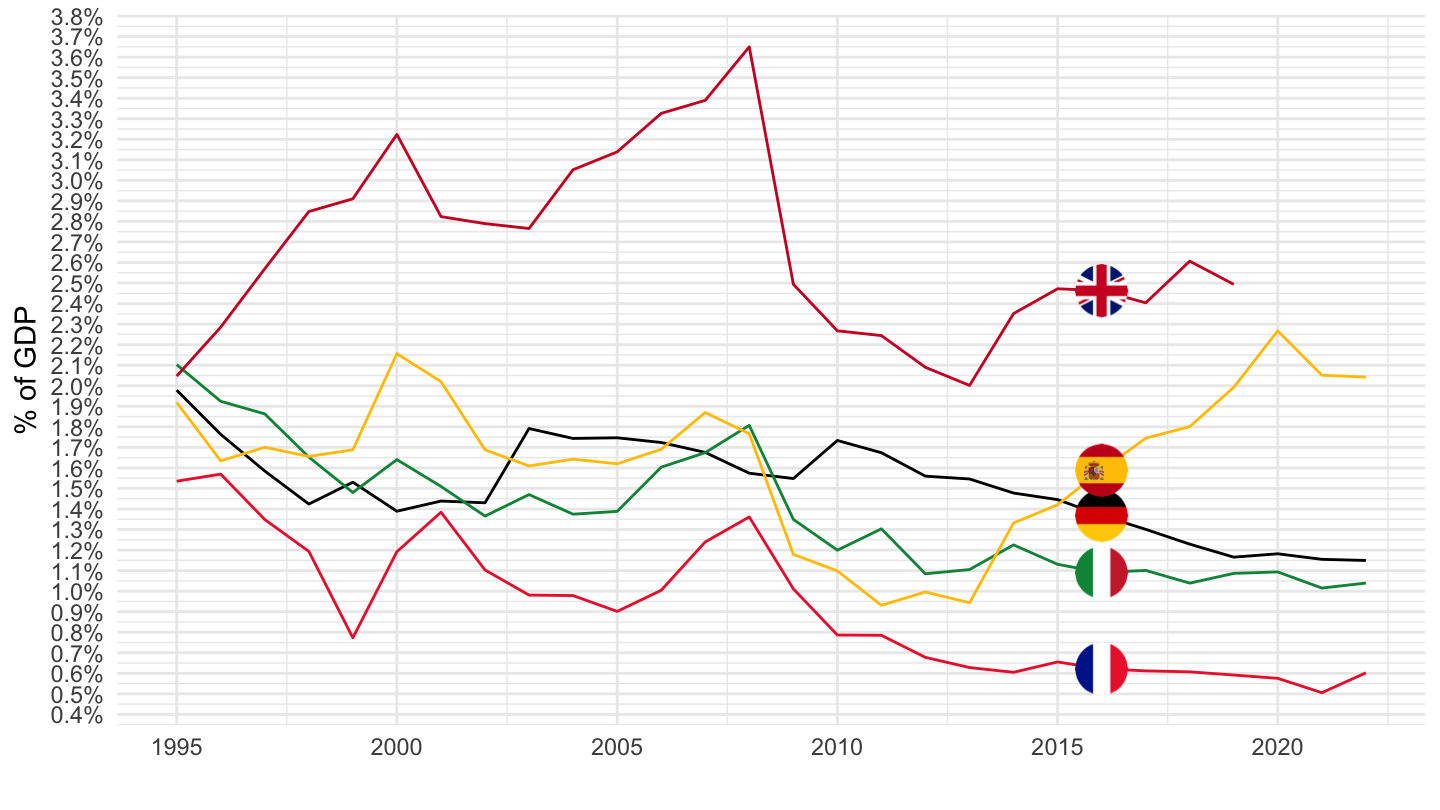
Aggregate Consumption (Nominal)
Table - Nominal - CP_MEUR
Code
nama_10_co3_p3 %>%
  filter(unit == "CP_MEUR",
         time %in% c("1995", "2005", "2019"),
         coicop == "TOTAL") %>%
  left_join(nama_10_gdp %>%
              filter(na_item == "B1GQ",
                     unit == "CP_MEUR") %>%
              select(geo, time, gdp = values),
            by = c("geo", "time")) %>%
  left_join(geo, by = "geo") %>%
  transmute(time, geo, Geo, values = 100*values/gdp) %>%
  spread(time, values) %>%
  mutate(Geo = ifelse(geo == "DE", "Germany", Geo)) %>%
  mutate(Flag = gsub(" ", "-", str_to_lower(Geo)),
         Flag = paste0('<img src="../../bib/flags/vsmall/', Flag, '.png" alt="Flag">')) %>%
  select(Flag, everything()) %>%
  arrange(`2019`) %>%
  {if (is_html_output()) datatable(., filter = 'top', rownames = F, escape = F) else .}
Table - Real - CLV15_MEUR
Code
nama_10_co3_p3 %>%
  filter(unit == "CLV15_MEUR",
         time %in% c("1995", "2005", "2019"),
         coicop == "TOTAL") %>%
  left_join(nama_10_gdp %>%
              filter(na_item == "B1GQ",
                     unit == "CLV15_MEUR") %>%
              select(geo, time, gdp = values),
            by = c("geo", "time")) %>%
  left_join(geo, by = "geo") %>%
  transmute(time, geo, Geo, values = 100*values/gdp) %>%
  spread(time, values) %>%
  mutate(Geo = ifelse(geo == "DE", "Germany", Geo)) %>%
  mutate(Flag = gsub(" ", "-", str_to_lower(Geo)),
         Flag = paste0('<img src="../../bib/flags/vsmall/', Flag, '.png" alt="Flag">')) %>%
  select(Flag, everything()) %>%
  arrange(`2019`) %>%
  {if (is_html_output()) datatable(., filter = 'top', rownames = F, escape = F) else .}
Denmark, Portugal, Sweden
All
Code
nama_10_co3_p3 %>%
  filter(unit == "CLV10_MEUR",
         geo %in% c("DK", "PT", "SE"),
         coicop == "TOTAL") %>%
  left_join(nama_10_gdp %>%
              filter(na_item == "B1GQ",
                     unit == "CLV10_MEUR") %>%
              select(geo, time, gdp = values),
            by = c("geo", "time")) %>%
  left_join(geo, by = "geo") %>%
  year_to_date %>%
  left_join(colors, by = c("Geo" = "country")) %>%
  mutate(values = values/gdp) %>%
  ggplot + geom_line(aes(x = date, y = values, color = color)) +
  theme_minimal()  + add_3flags +
  scale_color_identity() + xlab("") + ylab("% of GDP") +
  scale_x_date(breaks = as.Date(paste0(seq(1960, 2100, 2), "-01-01")),
               labels = date_format("%Y")) +
  theme(legend.position = c(0.2, 0.85),
        legend.title = element_blank()) +
  scale_y_continuous(breaks = 0.01*seq(0, 200, 1),
                     labels = scales::percent_format(accuracy = 1))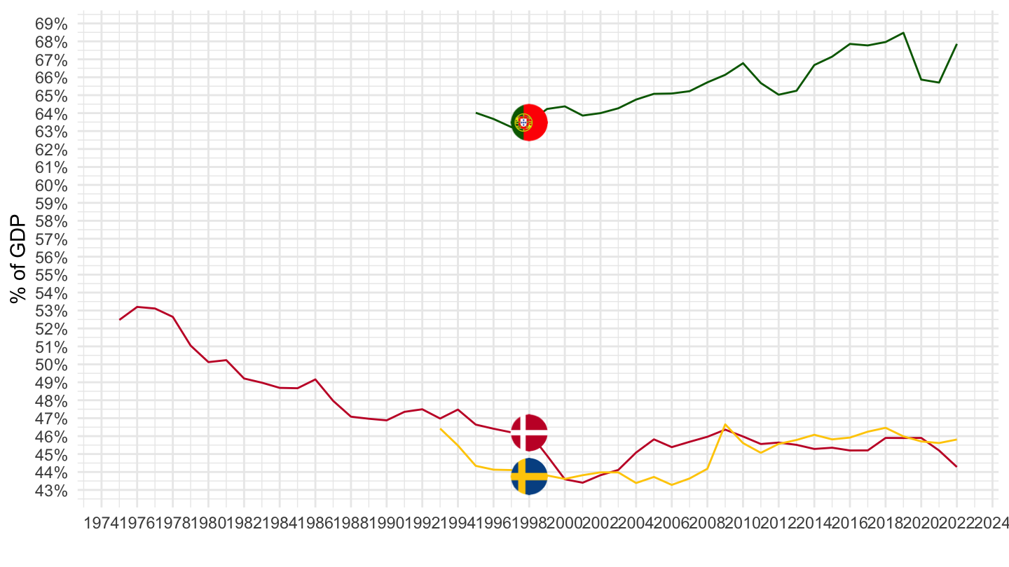
1995-
Code
nama_10_co3_p3 %>%
  filter(unit == "CLV10_MEUR",
         geo %in% c("DK", "PT", "SE"),
         coicop == "TOTAL") %>%
  left_join(nama_10_gdp %>%
              filter(na_item == "B1GQ",
                     unit == "CLV10_MEUR") %>%
              select(geo, time, gdp = values),
            by = c("geo", "time")) %>%
  left_join(geo, by = "geo") %>%
  year_to_date %>%
  filter(date >= as.Date("1995-01-01")) %>%
  left_join(colors, by = c("Geo" = "country")) %>%
  mutate(values = values/gdp) %>%
  ggplot + geom_line(aes(x = date, y = values, color = color)) +
  theme_minimal()  + add_3flags +
  scale_color_identity() + xlab("") + ylab("% of GDP") +
  scale_x_date(breaks = as.Date(paste0(seq(1960, 2100, 2), "-01-01")),
               labels = date_format("%Y")) +
  theme(legend.position = c(0.2, 0.85),
        legend.title = element_blank()) +
  scale_y_continuous(breaks = 0.01*seq(0, 200, 1),
                     labels = scales::percent_format(accuracy = 1))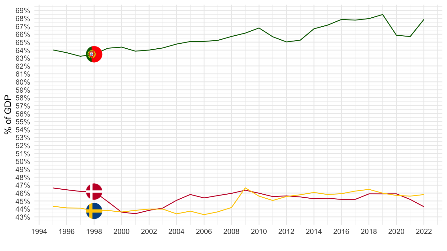
France - 2 digit
Housing, Transport, Food
% of GDP Volume
Code
nama_10_co3_p3 %>%
  filter(unit == "CLV10_MEUR",
         geo %in% c("FR"),
         coicop %in% c("CP04", "CP07", "CP01")) %>%
  left_join(nama_10_gdp %>%
              filter(na_item == "B1GQ") %>%
              select(geo, time, unit, gdp = values),
            by = c("geo", "time", "unit")) %>%
  left_join(coicop, by = "coicop") %>%
  year_to_date %>%
  ggplot + geom_line() + theme_minimal()  +
  aes(x = date, y = values/gdp, color = Coicop) +

  scale_x_date(breaks = as.Date(paste0(seq(1960, 2100, 5), "-01-01")),
               labels = date_format("%Y")) +
  theme(legend.position = c(0.3, 0.55),
        legend.title = element_blank()) +
  xlab("") + ylab("% of GDP") +
  scale_y_continuous(breaks = 0.01*seq(0, 200, 1),
                     labels = scales::percent_format(accuracy = 1))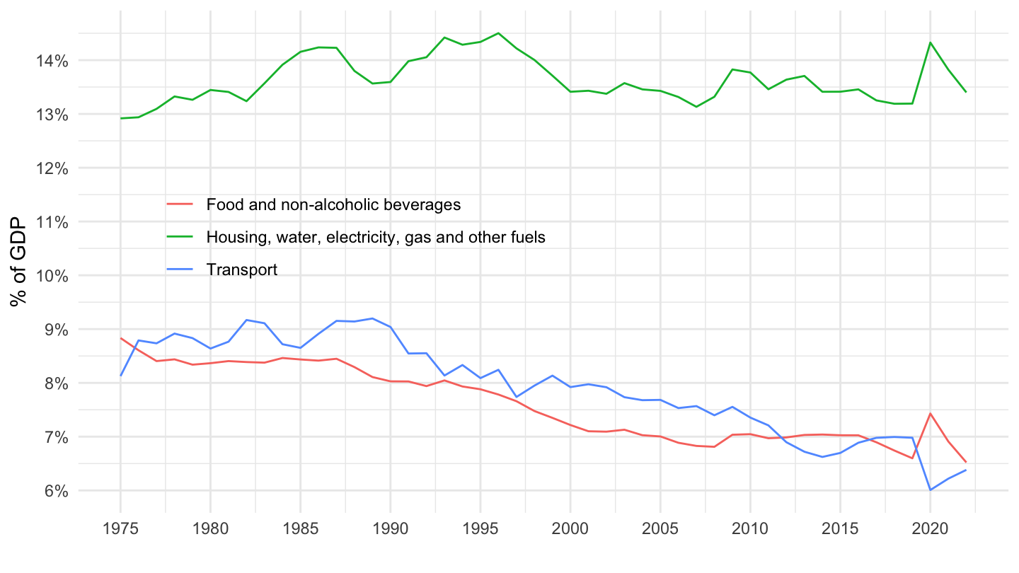
% of GDP Value
Code
nama_10_co3_p3 %>%
  filter(unit == "CP_MEUR",
         geo %in% c("FR"),
         coicop %in% c("CP04", "CP07", "CP01")) %>%
  left_join(nama_10_gdp %>%
              filter(na_item == "B1GQ") %>%
              select(geo, time, unit, gdp = values),
            by = c("geo", "time", "unit")) %>%
  left_join(coicop, by = "coicop") %>%
  year_to_date %>%
  ggplot + geom_line() + theme_minimal()  +
  aes(x = date, y = values/gdp, color = Coicop) +

  scale_x_date(breaks = as.Date(paste0(seq(1960, 2100, 5), "-01-01")),
               labels = date_format("%Y")) +
  theme(legend.position = c(0.3, 0.55),
        legend.title = element_blank()) +
  xlab("") + ylab("% of GDP") +
  scale_y_continuous(breaks = 0.01*seq(0, 200, 1),
                     labels = scales::percent_format(accuracy = 1))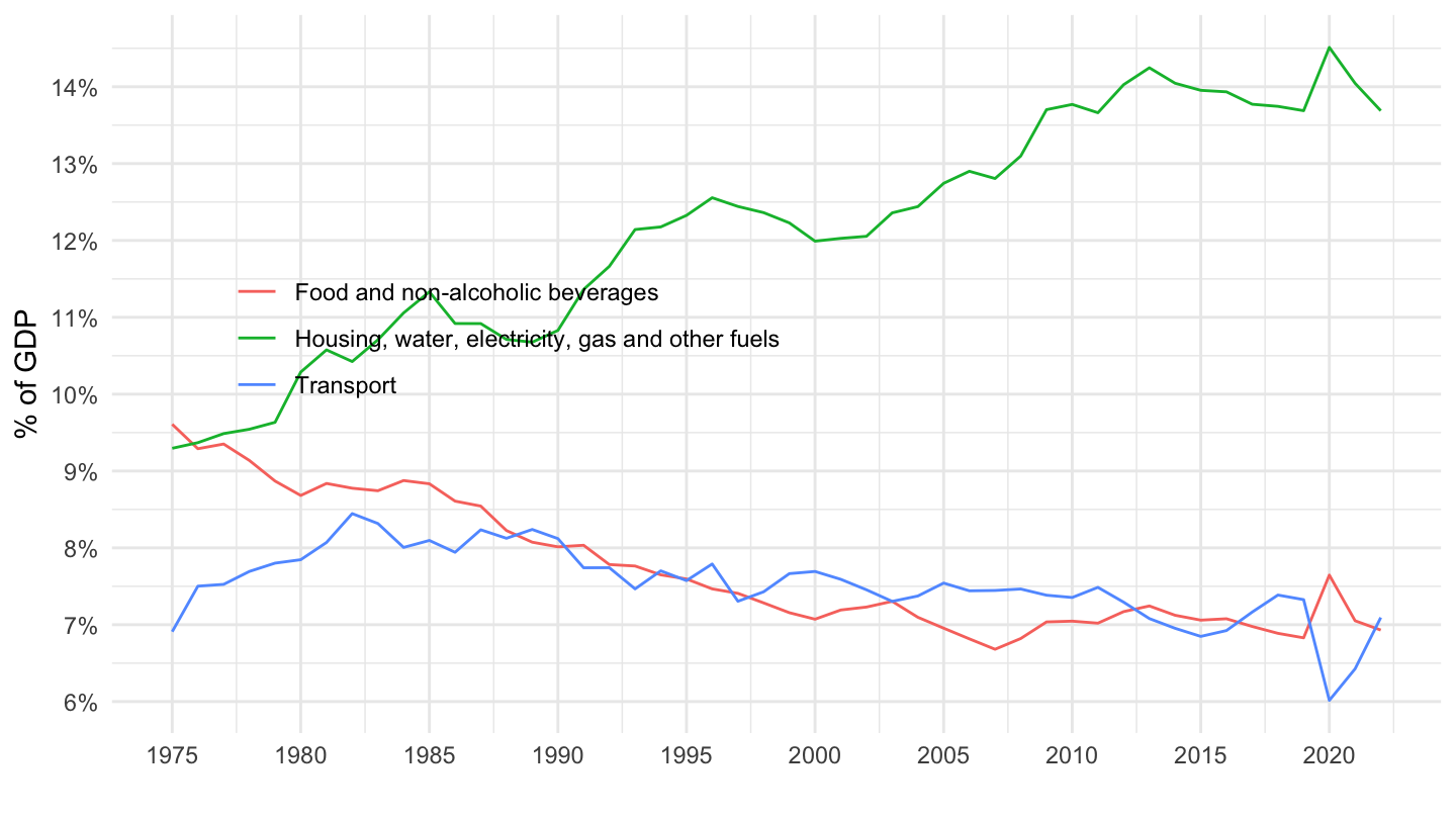
% of TOT
Code
nama_10_co3_p3 %>%
  filter(unit == "PC_TOT",
         geo %in% c("FR"),
         coicop %in% c("CP04", "CP07", "CP01")) %>%
  left_join(coicop, by = "coicop") %>%
  year_to_date %>%
  ggplot + geom_line() + theme_minimal()  +
  aes(x = date, y = values/100, color = Coicop) +

  scale_x_date(breaks = as.Date(paste0(seq(1960, 2100, 5), "-01-01")),
               labels = date_format("%Y")) +
  theme(legend.position = c(0.3, 0.85),
        legend.title = element_blank()) +
  xlab("") + ylab("% of GDP") +
  scale_y_continuous(breaks = 0.01*seq(0, 200, 1),
                     labels = scales::percent_format(accuracy = 1))
Misc, Recreation, Restaurants
Code
nama_10_co3_p3 %>%
  filter(unit == "CLV10_MEUR",
         geo %in% c("FR"),
         coicop %in% c("CP12", "CP09", "CP11")) %>%
  left_join(nama_10_gdp %>%
              filter(na_item == "B1GQ") %>%
              select(geo, time, unit, gdp = values),
            by = c("geo", "time", "unit")) %>%
  left_join(coicop, by = "coicop") %>%
  year_to_date %>%
  ggplot + geom_line() + theme_minimal()  +
  aes(x = date, y = values/gdp, color = Coicop) +

  scale_x_date(breaks = as.Date(paste0(seq(1960, 2100, 2), "-01-01")),
               labels = date_format("%Y")) +
  theme(legend.position = c(0.3, 0.9),
        legend.title = element_blank()) +
  xlab("") + ylab("% of GDP") +
  scale_y_continuous(breaks = 0.01*seq(0, 200, 0.5),
                     labels = scales::percent_format(accuracy = 0.1),
                     limits = c(0.02, 0.07))
Furnishings, Health, Communication
Code
nama_10_co3_p3 %>%
  filter(unit == "CLV10_MEUR",
         geo %in% c("FR"),
         coicop %in% c("CP05", "CP06", "CP08")) %>%
  left_join(nama_10_gdp %>%
              filter(na_item == "B1GQ") %>%
              select(geo, time, unit, gdp = values),
            by = c("geo", "time", "unit")) %>%
  left_join(coicop, by = "coicop") %>%
  year_to_date %>%
  ggplot + geom_line() + theme_minimal()  +
  aes(x = date, y = values/gdp, color = Coicop) +

  scale_x_date(breaks = as.Date(paste0(seq(1960, 2100, 2), "-01-01")),
               labels = date_format("%Y")) +
  theme(legend.position = c(0.35, 0.6),
        legend.title = element_blank()) +
  xlab("") + ylab("% of GDP") +
  scale_y_continuous(breaks = 0.01*seq(0, 200, 0.5),
                     labels = scales::percent_format(accuracy = 0.1))
Clothing, Alcohol, Education
Code
nama_10_co3_p3 %>%
  filter(unit == "CLV10_MEUR",
         geo %in% c("FR"),
         coicop %in% c("CP03", "CP02", "CP10")) %>%
  left_join(nama_10_gdp %>%
              filter(na_item == "B1GQ") %>%
              select(geo, time, unit, gdp = values),
            by = c("geo", "time", "unit")) %>%
  left_join(coicop, by = "coicop") %>%
  year_to_date %>%
  ggplot + geom_line() + theme_minimal()  +
  aes(x = date, y = values/gdp, color = Coicop) +

  scale_x_date(breaks = as.Date(paste0(seq(1960, 2100, 2), "-01-01")),
               labels = date_format("%Y")) +
  theme(legend.position = c(0.75, 0.9),
        legend.title = element_blank()) +
  xlab("") + ylab("% of GDP") +
  scale_y_continuous(breaks = 0.01*seq(0, 200, 0.5),
                     labels = scales::percent_format(accuracy = 0.1))
France - 2 digit (in French)
Housing, Transport, Food
Code
load_data("eurostat/coicop_fr.RData")
nama_10_co3_p3 %>%
  filter(unit == "CLV10_MEUR",
         geo %in% c("FR"),
         coicop %in% c("CP04", "CP07", "CP01")) %>%
  left_join(nama_10_gdp %>%
              filter(na_item == "B1GQ") %>%
              select(geo, time, unit, gdp = values),
            by = c("geo", "time", "unit")) %>%
  left_join(coicop, by = "coicop") %>%
  year_to_date %>%
  ggplot + geom_line() + theme_minimal()  +
  aes(x = date, y = values/gdp, color = Coicop) +

  scale_x_date(breaks = as.Date(paste0(seq(1960, 2100, 2), "-01-01")),
               labels = date_format("%Y")) +
  theme(legend.position = c(0.3, 0.55),
        legend.title = element_blank()) +
  xlab("") + ylab("% du PIB") +
  scale_y_continuous(breaks = 0.01*seq(0, 200, 1),
                     labels = scales::percent_format(accuracy = 1))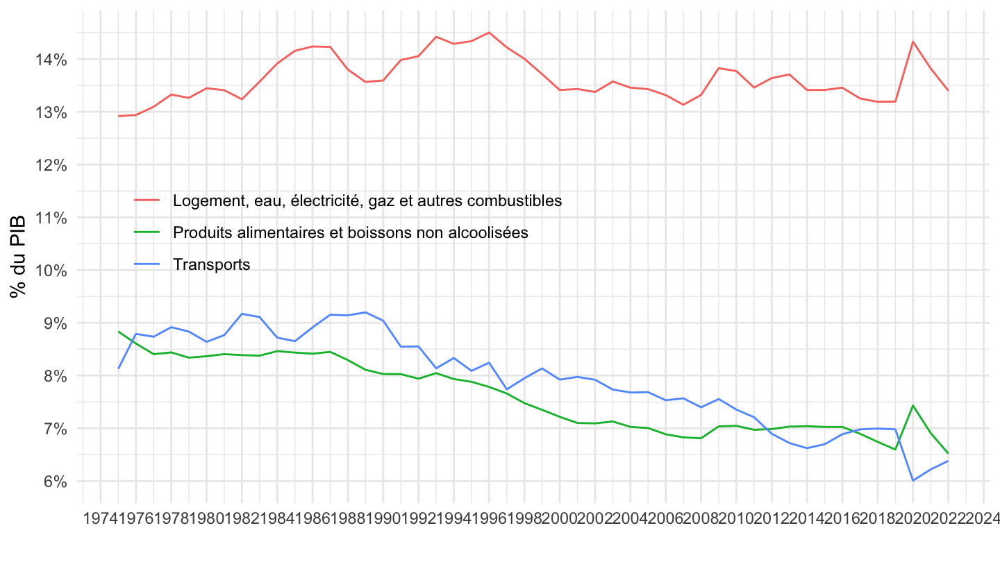
Misc, Recreation, Restaurants
Code
nama_10_co3_p3 %>%
  filter(unit == "CLV10_MEUR",
         geo %in% c("FR"),
         coicop %in% c("CP12", "CP09", "CP11")) %>%
  left_join(nama_10_gdp %>%
              filter(na_item == "B1GQ") %>%
              select(geo, time, unit, gdp = values),
            by = c("geo", "time", "unit")) %>%
  left_join(coicop, by = "coicop") %>%
  year_to_date %>%
  ggplot + geom_line() + theme_minimal()  +
  aes(x = date, y = values/gdp, color = Coicop) +

  scale_x_date(breaks = as.Date(paste0(seq(1960, 2100, 2), "-01-01")),
               labels = date_format("%Y")) +
  theme(legend.position = c(0.3, 0.9),
        legend.title = element_blank()) +
  xlab("") + ylab("% du PIB") +
  scale_y_continuous(breaks = 0.01*seq(0, 200, 0.5),
                     labels = scales::percent_format(accuracy = 0.1),
                     limits = c(0.02, 0.07))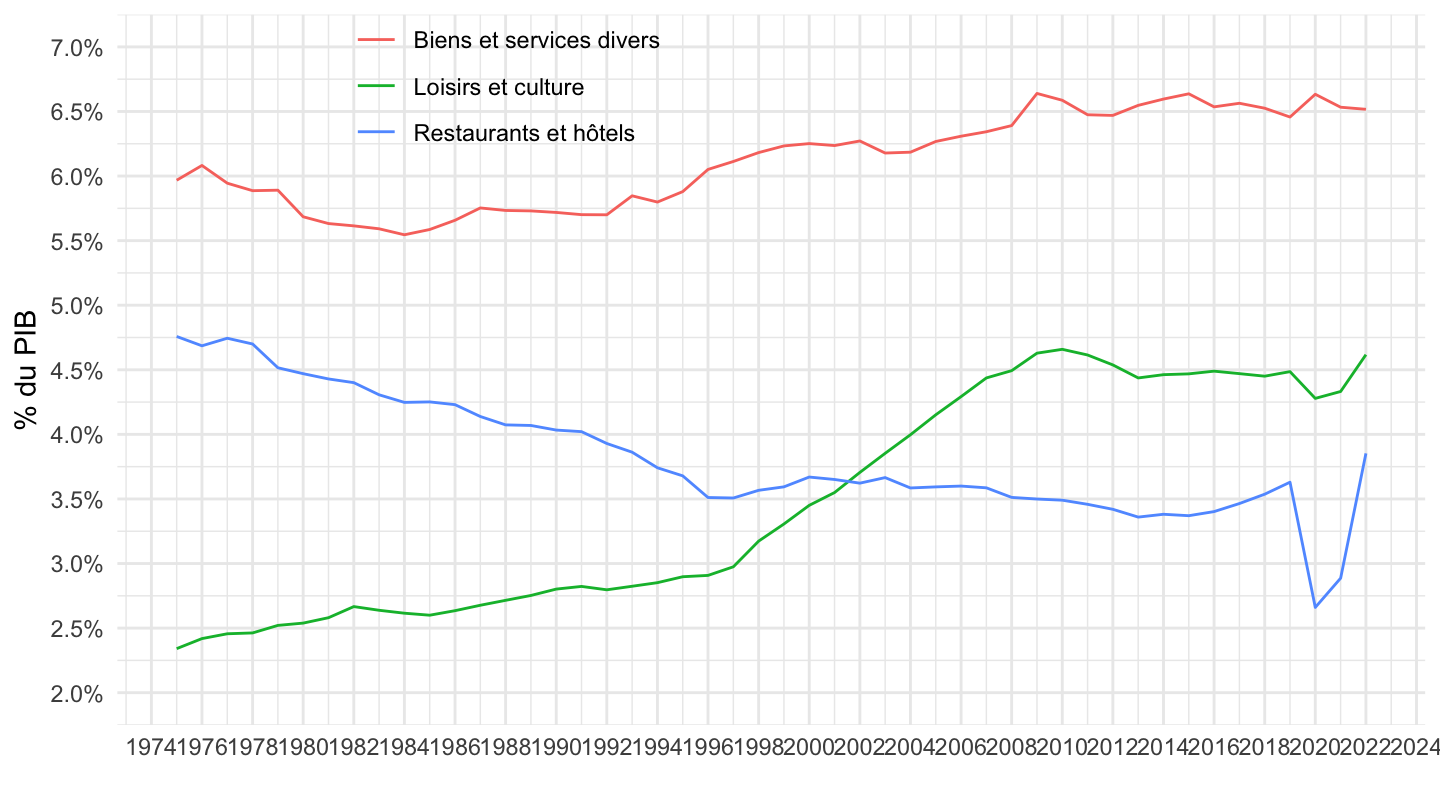
Furnishings, Health, Communication
Code
nama_10_co3_p3 %>%
  filter(unit == "CLV10_MEUR",
         geo %in% c("FR"),
         coicop %in% c("CP05", "CP06", "CP08")) %>%
  left_join(nama_10_gdp %>%
              filter(na_item == "B1GQ") %>%
              select(geo, time, unit, gdp = values),
            by = c("geo", "time", "unit")) %>%
  left_join(coicop, by = "coicop") %>%
  year_to_date %>%
  ggplot + geom_line() + theme_minimal()  +
  aes(x = date, y = values/gdp, color = Coicop) +

  scale_x_date(breaks = as.Date(paste0(seq(1960, 2100, 2), "-01-01")),
               labels = date_format("%Y")) +
  theme(legend.position = c(0.35, 0.6),
        legend.title = element_blank()) +
  xlab("") + ylab("% du GDP") +
  scale_y_continuous(breaks = 0.01*seq(0, 200, 0.5),
                     labels = scales::percent_format(accuracy = 0.1))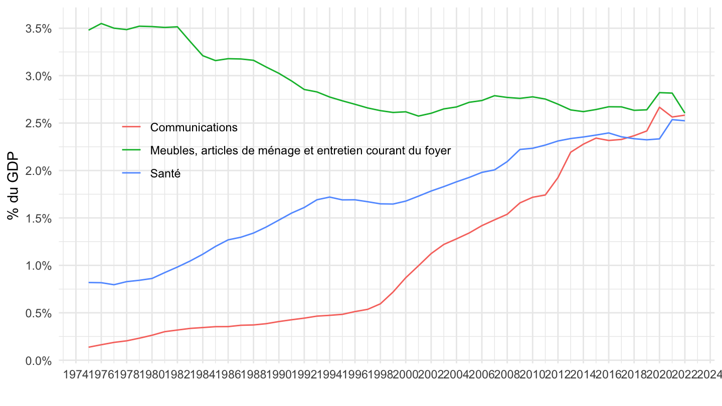
Clothing, Alcohol, Education
Code
nama_10_co3_p3 %>%
  filter(unit == "CLV10_MEUR",
         geo %in% c("FR"),
         coicop %in% c("CP03", "CP02", "CP10")) %>%
  left_join(nama_10_gdp %>%
              filter(na_item == "B1GQ") %>%
              select(geo, time, unit, gdp = values),
            by = c("geo", "time", "unit")) %>%
  left_join(coicop, by = "coicop") %>%
  year_to_date %>%
  ggplot + geom_line() + theme_minimal()  +
  aes(x = date, y = values/gdp, color = Coicop) +

  scale_x_date(breaks = as.Date(paste0(seq(1960, 2100, 2), "-01-01")),
               labels = date_format("%Y")) +
  theme(legend.position = c(0.75, 0.9),
        legend.title = element_blank()) +
  xlab("") + ylab("% du PIB") +
  scale_y_continuous(breaks = 0.01*seq(0, 200, 0.5),
                     labels = scales::percent_format(accuracy = 0.1))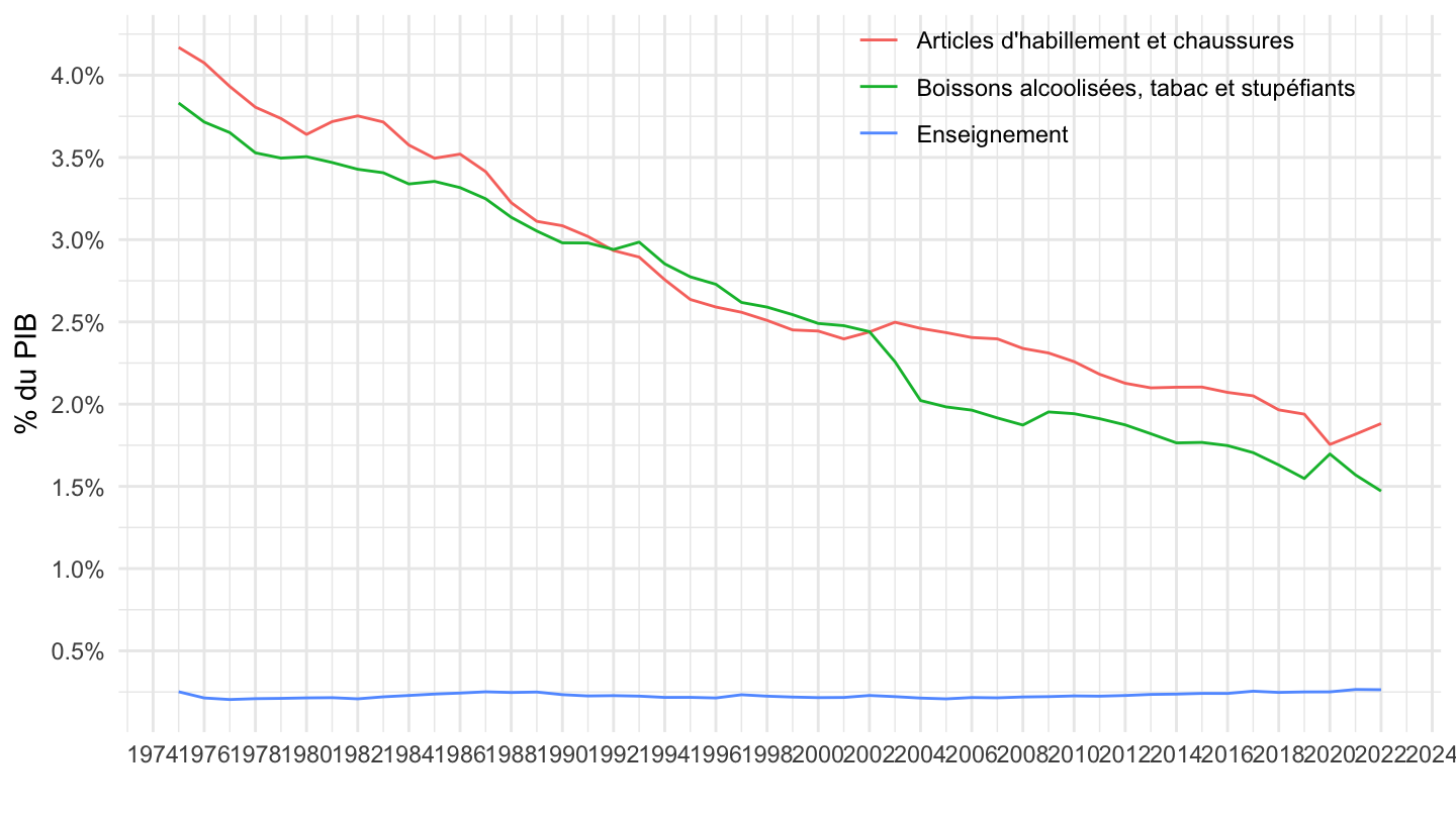
France - 3 digit
Food, non alcoholic
Code
load_data("eurostat/coicop.RData")
nama_10_co3_p3 %>%
  filter(unit == "CLV10_MEUR",
         geo %in% c("FR"),
         coicop %in% c("CP011", "CP012")) %>%
  left_join(nama_10_gdp %>%
              filter(na_item == "B1GQ") %>%
              select(geo, time, unit, gdp = values),
            by = c("geo", "time", "unit")) %>%
  left_join(coicop, by = "coicop") %>%
  year_to_date %>%
  ggplot + geom_line() + theme_minimal()  +
  aes(x = date, y = values/gdp, color = Coicop) +

  scale_x_date(breaks = as.Date(paste0(seq(1960, 2100, 2), "-01-01")),
               labels = date_format("%Y")) +
  theme(legend.position = c(0.3, 0.55),
        legend.title = element_blank()) +
  xlab("") + ylab("% of GDP") +
  scale_y_continuous(breaks = 0.01*seq(0, 200, 1),
                     labels = scales::percent_format(accuracy = 1))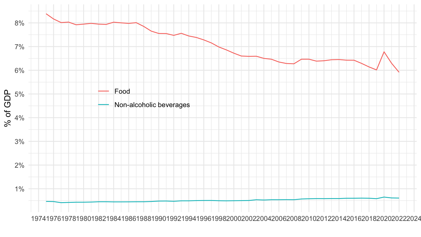
Alcohol, Tobacco, Narcotics
Code
nama_10_co3_p3 %>%
  filter(unit == "CLV10_MEUR",
         geo %in% c("FR"),
         coicop %in% c("CP021", "CP022", "CP023")) %>%
  left_join(nama_10_gdp %>%
              filter(na_item == "B1GQ") %>%
              select(geo, time, unit, gdp = values),
            by = c("geo", "time", "unit")) %>%
  left_join(coicop, by = "coicop") %>%
  year_to_date %>%
  ggplot + geom_line() + theme_minimal()  +
  aes(x = date, y = values/gdp, color = Coicop) +

  scale_x_date(breaks = as.Date(paste0(seq(1960, 2100, 2), "-01-01")),
               labels = date_format("%Y")) +
  theme(legend.position = c(0.8, 0.85),
        legend.title = element_blank()) +
  xlab("") + ylab("% of GDP") +
  scale_y_continuous(breaks = 0.01*seq(0, 200, 0.2),
                     labels = scales::percent_format(accuracy = 0.1))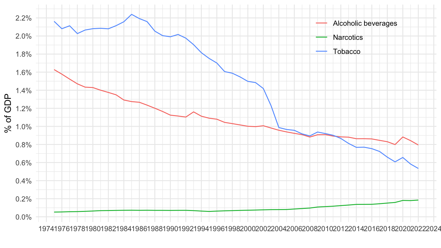
Clothing, Footware
Code
nama_10_co3_p3 %>%
  filter(unit == "CLV10_MEUR",
         geo %in% c("FR"),
         coicop %in% c("CP031", "CP032")) %>%
  left_join(nama_10_gdp %>%
              filter(na_item == "B1GQ") %>%
              select(geo, time, unit, gdp = values),
            by = c("geo", "time", "unit")) %>%
  left_join(coicop, by = "coicop") %>%
  year_to_date %>%
  ggplot + geom_line() + theme_minimal()  +
  aes(x = date, y = values/gdp, color = Coicop) +

  scale_x_date(breaks = as.Date(paste0(seq(1960, 2100, 2), "-01-01")),
               labels = date_format("%Y")) +
  theme(legend.position = c(0.9, 0.85),
        legend.title = element_blank()) +
  xlab("") + ylab("% of GDP") +
  scale_y_continuous(breaks = 0.01*seq(0, 200, 0.5),
                     labels = scales::percent_format(accuracy = 1))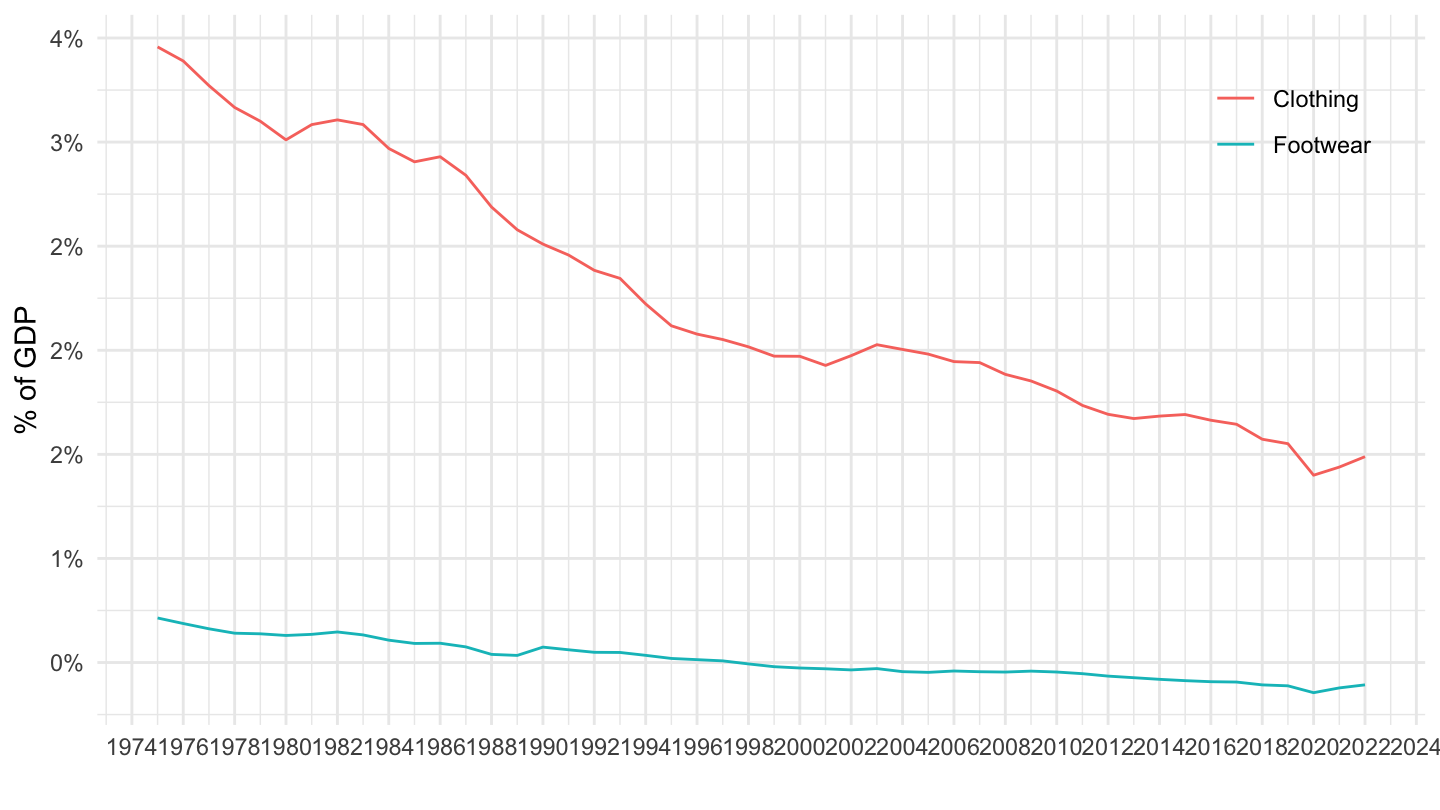
Housing 1/2
Code
nama_10_co3_p3 %>%
  filter(unit == "CLV10_MEUR",
         geo %in% c("FR"),
         coicop %in% c("CP041", "CP042", "CP043")) %>%
  left_join(nama_10_gdp %>%
              filter(na_item == "B1GQ") %>%
              select(geo, time, unit, gdp = values),
            by = c("geo", "time", "unit")) %>%
  left_join(coicop, by = "coicop") %>%
  year_to_date %>%
  ggplot + geom_line() + theme_minimal()  +
  aes(x = date, y = values/gdp, color = Coicop) +

  scale_x_date(breaks = as.Date(paste0(seq(1960, 2100, 2), "-01-01")),
               labels = date_format("%Y")) +
  theme(legend.position = c(0.7, 0.55),
        legend.title = element_blank()) +
  xlab("") + ylab("% of GDP") +
  scale_y_continuous(breaks = 0.01*seq(0, 200, 1),
                     labels = scales::percent_format(accuracy = 1))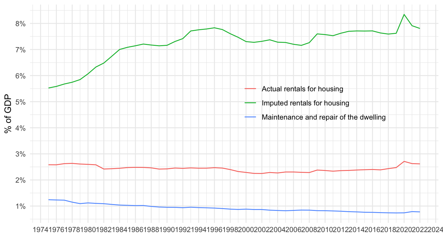
Housing 2/2
Code
nama_10_co3_p3 %>%
  filter(unit == "CLV10_MEUR",
         geo %in% c("FR"),
         coicop %in% c("CP044", "CP045", "CP046")) %>%
  left_join(nama_10_gdp %>%
              filter(na_item == "B1GQ") %>%
              select(geo, time, unit, gdp = values),
            by = c("geo", "time", "unit")) %>%
  left_join(coicop, by = "coicop") %>%
  year_to_date %>%
  ggplot + geom_line() + theme_minimal()  +
  aes(x = date, y = values/gdp, color = Coicop) +

  scale_x_date(breaks = as.Date(paste0(seq(1960, 2100, 2), "-01-01")),
               labels = date_format("%Y")) +
  theme(legend.position = c(0.4, 0.55),
        legend.title = element_blank()) +
  xlab("") + ylab("% of GDP") +
  scale_y_continuous(breaks = 0.01*seq(0, 200, .2),
                     labels = scales::percent_format(accuracy = .1))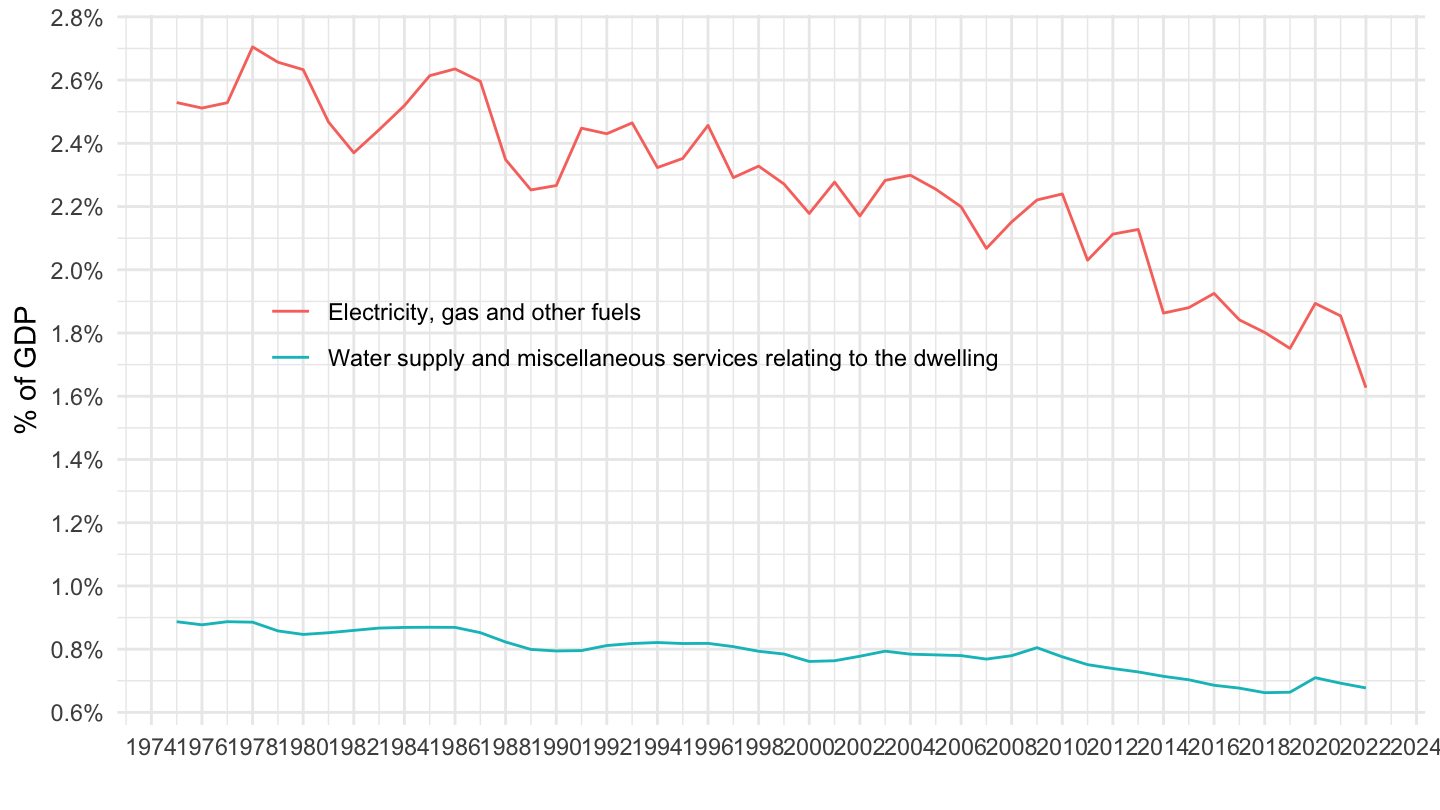
Furniture 1/2
Code
nama_10_co3_p3 %>%
  filter(unit == "CLV10_MEUR",
         geo %in% c("FR"),
         coicop %in% c("CP051", "CP052", "CP053")) %>%
  left_join(nama_10_gdp %>%
              filter(na_item == "B1GQ") %>%
              select(geo, time, unit, gdp = values),
            by = c("geo", "time", "unit")) %>%
  left_join(coicop, by = "coicop") %>%
  year_to_date %>%
  ggplot + geom_line() + theme_minimal()  +
  aes(x = date, y = values/gdp, color = Coicop) +

  scale_x_date(breaks = as.Date(paste0(seq(1960, 2100, 2), "-01-01")),
               labels = date_format("%Y")) +
  theme(legend.position = c(0.7, 0.85),
        legend.title = element_blank()) +
  xlab("") + ylab("% of GDP") +
  scale_y_continuous(breaks = 0.01*seq(0, 200, 0.1),
                     labels = scales::percent_format(accuracy = .1))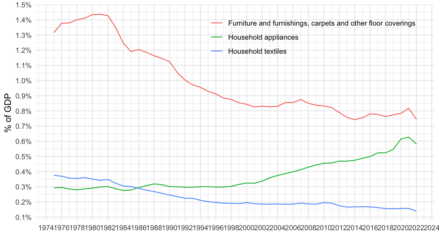
Furniture 1/2
Code
nama_10_co3_p3 %>%
  filter(unit == "CLV10_MEUR",
         geo %in% c("FR"),
         coicop %in% c("CP054", "CP055", "CP056")) %>%
  left_join(nama_10_gdp %>%
              filter(na_item == "B1GQ") %>%
              select(geo, time, unit, gdp = values),
            by = c("geo", "time", "unit")) %>%
  left_join(coicop, by = "coicop") %>%
  year_to_date %>%
  ggplot + geom_line() + theme_minimal()  +
  aes(x = date, y = values/gdp, color = Coicop) +

  scale_x_date(breaks = as.Date(paste0(seq(1960, 2100, 2), "-01-01")),
               labels = date_format("%Y")) +
  theme(legend.position = c(0.7, 0.9),
        legend.title = element_blank()) +
  xlab("") + ylab("% of GDP") +
  scale_y_continuous(breaks = 0.01*seq(0, 200, 0.1),
                     labels = scales::percent_format(accuracy = .1))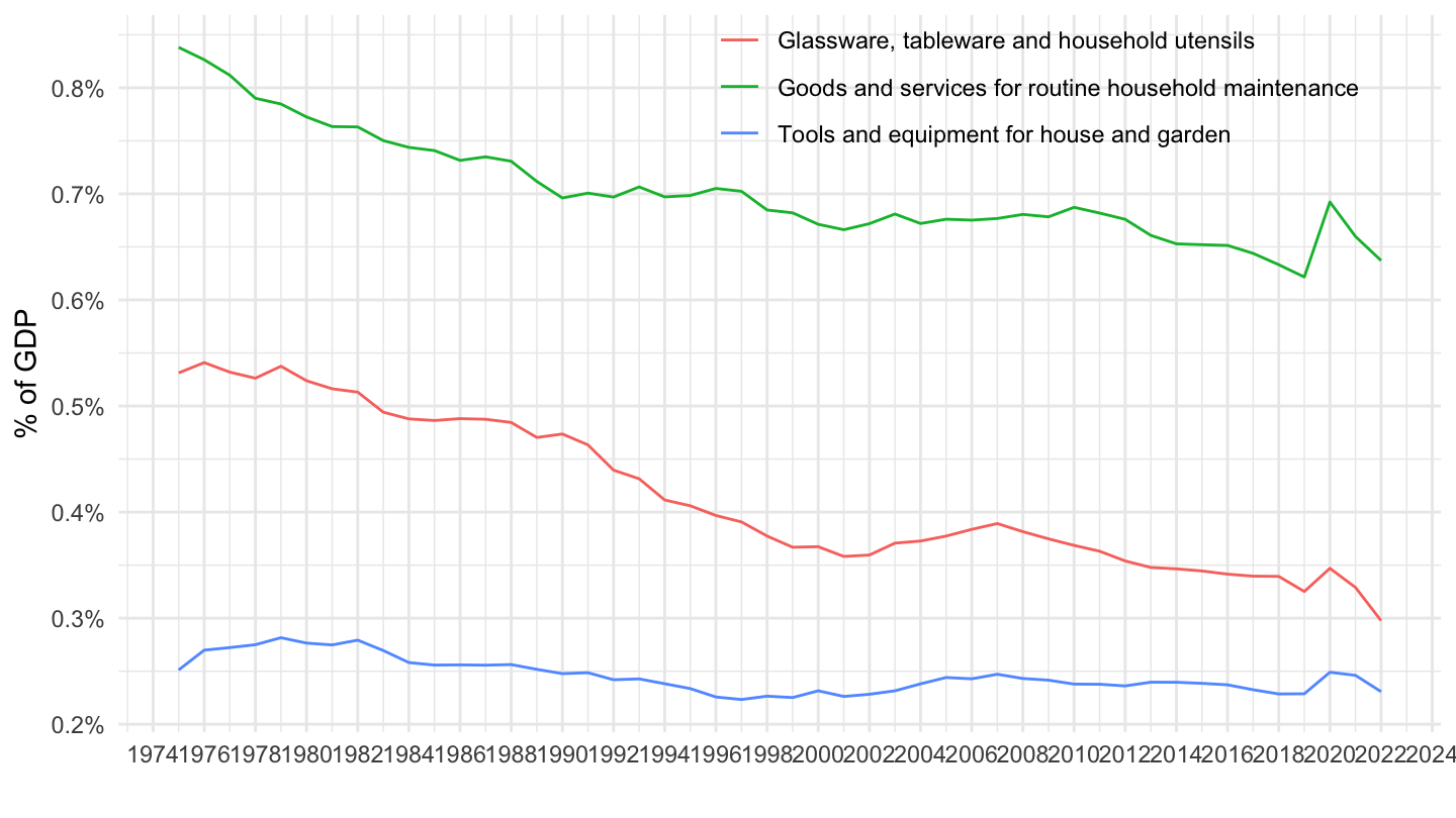
Medical
Code
nama_10_co3_p3 %>%
  filter(unit == "CLV10_MEUR",
         geo %in% c("FR"),
         coicop %in% c("CP061", "CP062", "CP063")) %>%
  left_join(nama_10_gdp %>%
              filter(na_item == "B1GQ") %>%
              select(geo, time, unit, gdp = values),
            by = c("geo", "time", "unit")) %>%
  left_join(coicop, by = "coicop") %>%
  year_to_date %>%
  ggplot + geom_line() + theme_minimal()  +
  aes(x = date, y = values/gdp, color = Coicop) +

  scale_x_date(breaks = as.Date(paste0(seq(1960, 2100, 2), "-01-01")),
               labels = date_format("%Y")) +
  theme(legend.position = c(0.3, 0.85),
        legend.title = element_blank()) +
  xlab("") + ylab("% of GDP") +
  scale_y_continuous(breaks = 0.01*seq(0, 200, 0.1),
                     labels = scales::percent_format(accuracy = .1))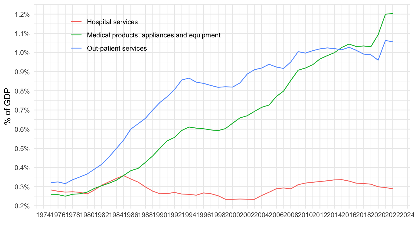
Operation, Vehicles, Transport
Code
nama_10_co3_p3 %>%
  filter(unit == "CLV10_MEUR",
         geo %in% c("FR"),
         coicop %in% c("CP071", "CP072", "CP073")) %>%
  left_join(nama_10_gdp %>%
              filter(na_item == "B1GQ") %>%
              select(geo, time, unit, gdp = values),
            by = c("geo", "time", "unit")) %>%
  left_join(coicop, by = "coicop") %>%
  year_to_date %>%
  ggplot + geom_line() + theme_minimal()  +
  aes(x = date, y = values/gdp, color = Coicop) +

  scale_x_date(breaks = as.Date(paste0(seq(1960, 2100, 2), "-01-01")),
               labels = date_format("%Y")) +
  theme(legend.position = c(0.8, 0.85),
        legend.title = element_blank()) +
  xlab("") + ylab("% of GDP") +
  scale_y_continuous(breaks = 0.01*seq(0, 200, 0.5),
                     labels = scales::percent_format(accuracy = .1))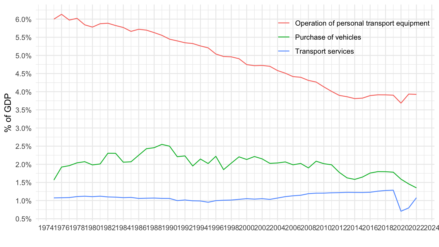
Postal, Telephone
Code
nama_10_co3_p3 %>%
  filter(unit == "CLV10_MEUR",
         geo %in% c("FR"),
         coicop %in% c("CP081", "CP082", "CP083")) %>%
  left_join(nama_10_gdp %>%
              filter(na_item == "B1GQ") %>%
              select(geo, time, unit, gdp = values),
            by = c("geo", "time", "unit")) %>%
  left_join(coicop, by = "coicop") %>%
  year_to_date %>%
  ggplot + geom_line() + theme_minimal()  +
  aes(x = date, y = values/gdp, color = Coicop) +

  scale_x_date(breaks = as.Date(paste0(seq(1960, 2100, 2), "-01-01")),
               labels = date_format("%Y")) +
  theme(legend.position = c(0.3, 0.85),
        legend.title = element_blank()) +
  xlab("") + ylab("% of GDP") +
  scale_y_continuous(breaks = 0.01*seq(0, 200, 0.2),
                     labels = scales::percent_format(accuracy = .1))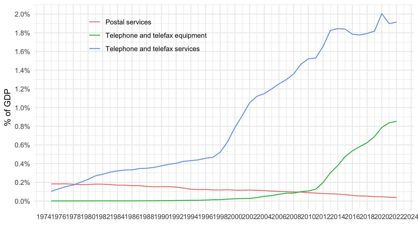
Audio-visual, other durables
Code
nama_10_co3_p3 %>%
  filter(unit == "CLV10_MEUR",
         geo %in% c("FR"),
         coicop %in% c("CP091", "CP092", "CP093")) %>%
  left_join(nama_10_gdp %>%
              filter(na_item == "B1GQ") %>%
              select(geo, time, unit, gdp = values),
            by = c("geo", "time", "unit")) %>%
  left_join(coicop, by = "coicop") %>%
  year_to_date %>%
  ggplot + geom_line() + theme_minimal()  +
  aes(x = date, y = values/gdp, color = Coicop) +

  scale_x_date(breaks = as.Date(paste0(seq(1960, 2100, 2), "-01-01")),
               labels = date_format("%Y")) +
  theme(legend.position = c(0.3, 0.85),
        legend.title = element_blank()) +
  xlab("") + ylab("% of GDP") +
  scale_y_continuous(breaks = 0.01*seq(0, 200, 0.2),
                     labels = scales::percent_format(accuracy = .1))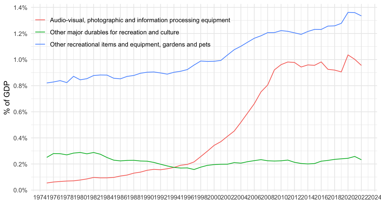
Newspapers, Package holidays
Code
nama_10_co3_p3 %>%
  filter(unit == "CLV10_MEUR",
         geo %in% c("FR"),
         coicop %in% c("CP094", "CP095", "CP096")) %>%
  left_join(nama_10_gdp %>%
              filter(na_item == "B1GQ") %>%
              select(geo, time, unit, gdp = values),
            by = c("geo", "time", "unit")) %>%
  left_join(coicop, by = "coicop") %>%
  year_to_date %>%
  ggplot + geom_line() + theme_minimal()  +
  aes(x = date, y = values/gdp, color = Coicop) +

  scale_x_date(breaks = as.Date(paste0(seq(1960, 2100, 2), "-01-01")),
               labels = date_format("%Y")) +
  theme(legend.position = c(0.2, 0.45),
        legend.title = element_blank()) +
  xlab("") + ylab("% of GDP") +
  scale_y_continuous(breaks = 0.01*seq(0, 200, 0.2),
                     labels = scales::percent_format(accuracy = .1))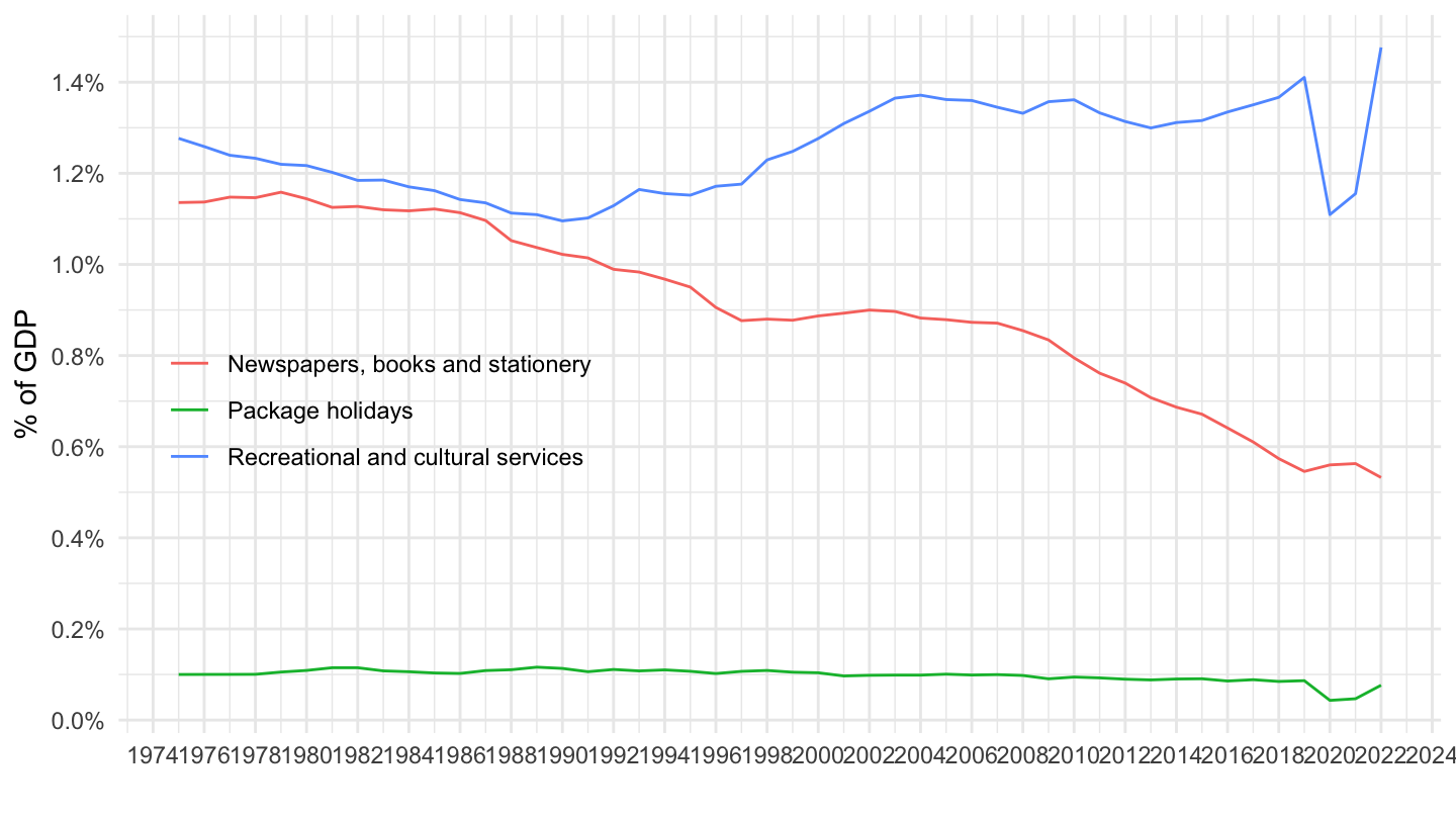
Education
Code
nama_10_co3_p3 %>%
  filter(unit == "CLV10_MEUR",
         geo %in% c("FR"),
         coicop %in% c("CP101", "CP102", "CP104", "CP105")) %>%
  left_join(nama_10_gdp %>%
              filter(na_item == "B1GQ") %>%
              select(geo, time, unit, gdp = values),
            by = c("geo", "time", "unit")) %>%
  left_join(coicop, by = "coicop") %>%
  year_to_date %>%
  ggplot + geom_line() + theme_minimal()  +
  aes(x = date, y = values/gdp, color = Coicop) +

  scale_x_date(breaks = as.Date(paste0(seq(1960, 2100, 2), "-01-01")),
               labels = date_format("%Y")) +
  theme(legend.position = c(0.8, 0.85),
        legend.title = element_blank()) +
  xlab("") + ylab("% of GDP") +
  scale_y_continuous(breaks = 0.01*seq(0, 200, 0.01),
                     labels = scales::percent_format(accuracy = .01))
Accommodation, catering
Code
nama_10_co3_p3 %>%
  filter(unit == "CLV10_MEUR",
         geo %in% c("FR"),
         coicop %in% c("CP111", "CP112")) %>%
  left_join(nama_10_gdp %>%
              filter(na_item == "B1GQ") %>%
              select(geo, time, unit, gdp = values),
            by = c("geo", "time", "unit")) %>%
  left_join(coicop, by = "coicop") %>%
  year_to_date %>%
  ggplot + geom_line() + theme_minimal()  +
  aes(x = date, y = values/gdp, color = Coicop) +

  scale_x_date(breaks = as.Date(paste0(seq(1960, 2100, 2), "-01-01")),
               labels = date_format("%Y")) +
  theme(legend.position = c(0.8, 0.85),
        legend.title = element_blank()) +
  xlab("") + ylab("% of GDP") +
  scale_y_continuous(breaks = 0.01*seq(0, 200, 0.5),
                     labels = scales::percent_format(accuracy = .1))
Finance, Insurance
Code
nama_10_co3_p3 %>%
  filter(unit == "CLV10_MEUR",
         geo %in% c("FR"),
         coicop %in% c("CP121", "CP124", "CP125", "CP126")) %>%
  left_join(nama_10_gdp %>%
              filter(na_item == "B1GQ") %>%
              select(geo, time, unit, gdp = values),
            by = c("geo", "time", "unit")) %>%
  left_join(coicop, by = "coicop") %>%
  year_to_date %>%
  ggplot + geom_line() + theme_minimal()  +
  aes(x = date, y = values/gdp, color = Coicop) +

  scale_x_date(breaks = as.Date(paste0(seq(1960, 2100, 2), "-01-01")),
               labels = date_format("%Y")) +
  theme(legend.position = c(0.2, 0.85),
        legend.title = element_blank()) +
  xlab("") + ylab("% of GDP") +
  scale_y_continuous(breaks = 0.01*seq(0, 200, 0.2),
                     labels = scales::percent_format(accuracy = .1))