Consumer Expectations Survey
Data - ECB
Info
Data on inflation
| source | dataset | Title | .html | .rData |
|---|---|---|---|---|
| ecb | CES | Consumer Expectations Survey | 2026-07-23 | 2026-07-19 |
| bis | CPI | Consumer Price Index | 2026-07-22 | 2026-07-22 |
| eurostat | nama_10_co3_p3 | Final consumption expenditure of households by consumption purpose (COICOP 3 digit) | 2026-07-18 | 2026-07-23 |
| eurostat | prc_hicp_cow | HICP - country weights | 2026-07-23 | 2026-07-23 |
| eurostat | prc_hicp_ctrb | Contributions to euro area annual inflation (in percentage points) | 2026-07-23 | 2026-07-23 |
| eurostat | prc_hicp_inw | HICP - item weights | 2026-07-23 | 2026-07-23 |
| eurostat | prc_hicp_manr | HICP (2015 = 100) - monthly data (annual rate of change) | 2026-07-23 | 2026-07-23 |
| eurostat | prc_hicp_midx | HICP (2015 = 100) - monthly data (index) | 2026-07-23 | 2026-07-23 |
| eurostat | prc_hicp_mmor | HICP (2015 = 100) - monthly data (monthly rate of change) | 2026-07-23 | 2026-07-23 |
| eurostat | prc_ppp_ind | Purchasing power parities (PPPs), price level indices and real expenditures for ESA 2010 aggregates | 2026-07-22 | 2026-07-23 |
| eurostat | sts_inpp_m | Producer prices in industry, total - monthly data | 2026-07-21 | 2026-07-23 |
| eurostat | sts_inppd_m | Producer prices in industry, domestic market - monthly data | 2026-07-21 | 2026-07-23 |
| eurostat | sts_inppnd_m | Producer prices in industry, non domestic market - monthly data | 2026-07-21 | 2026-07-23 |
| fred | cpi | Consumer Price Index | 2026-07-22 | 2026-07-22 |
| fred | inflation | Inflation | 2026-07-22 | 2026-07-22 |
| imf | CPI | Consumer Price Index (CPI) 2026 February - CPI_2026_FEB_VINTAGE | 2026-07-22 | 2026-04-13 |
| oecd | MEI_PRICES_PPI | Producer Prices - MEI_PRICES_PPI | 2026-07-23 | 2024-04-15 |
| oecd | PPP2017 | 2017 PPP Benchmark results | 2024-04-16 | 2023-07-25 |
| oecd | PRICES_CPI | Consumer price indices (CPIs) | 2024-04-16 | 2024-04-15 |
| wdi | FP.CPI.TOTL.ZG | Inflation, consumer prices (annual %) | 2026-07-22 | 2026-07-22 |
| wdi | NY.GDP.DEFL.KD.ZG | Inflation, GDP deflator (annual %) | 2026-07-22 | 2026-07-22 |
Données sur l’inflation en France
| source | dataset | Title | .html | .rData |
|---|---|---|---|---|
| insee | ILC-ILAT-ICC | Indices pour la révision d’un bail commercial ou professionnel | 2026-07-23 | 2026-07-23 |
| insee | INDICES_LOYERS | Indices des loyers d'habitation (ILH) | 2026-07-23 | 2026-07-23 |
| insee | IPC-1970-1980 | Indice des prix à la consommation - Base 1970, 1980 | 2026-07-23 | 2026-07-23 |
| insee | IPC-1990 | Indices des prix à la consommation - Base 1990 | 2026-07-23 | 2026-07-23 |
| insee | IPC-2015 | Indice des prix à la consommation - Base 2015 | 2026-07-23 | 2026-07-23 |
| insee | IPC-PM-2015 | Prix moyens de vente de détail | 2026-07-23 | 2026-07-23 |
| insee | IPCH-2015 | Indices des prix à la consommation harmonisés | 2026-07-23 | 2026-07-23 |
| insee | IPCH-IPC-2015-ensemble | Indices des prix à la consommation harmonisés | 2026-07-23 | 2026-07-23 |
| insee | IPGD-2015 | Indice des prix dans la grande distribution | 2026-07-23 | 2026-07-23 |
| insee | IPLA-IPLNA-2015 | Indices des prix des logements neufs et Indices Notaires-Insee des prix des logements anciens | 2026-07-23 | 2026-07-23 |
| insee | IPPI-2015 | Indices de prix de production et d'importation dans l'industrie | 2026-07-23 | 2026-07-23 |
| insee | IRL | Indice pour la révision d’un loyer d’habitation | 2026-07-23 | 2026-07-23 |
| insee | SERIES_LOYERS | Variation des loyers | 2026-07-23 | 2026-07-23 |
| insee | T_CONSO_EFF_FONCTION | Consommation effective des ménages par fonction | 2026-07-23 | 2025-12-22 |
| insee | bdf2017 | Budget de famille 2017 | 2026-07-23 | 2023-11-21 |
| insee | echantillon-agglomerations-IPC-2024 | Échantillon d’agglomérations enquêtées de l’IPC en 2024 | 2026-07-23 | 2026-01-27 |
| insee | echantillon-agglomerations-IPC-2025 | Échantillon d’agglomérations enquêtées de l’IPC en 2025 | 2026-07-23 | 2026-01-27 |
| insee | liste-varietes-IPC-2024 | Liste des variétés pour la mesure de l'IPC en 2024 | 2026-07-23 | 2025-04-02 |
| insee | liste-varietes-IPC-2025 | Liste des variétés pour la mesure de l'IPC en 2025 | 2026-07-23 | 2026-01-27 |
| insee | ponderations-elementaires-IPC-2024 | Pondérations élémentaires 2024 intervenant dans le calcul de l’IPC | 2026-07-23 | 2025-04-02 |
| insee | ponderations-elementaires-IPC-2025 | Pondérations élémentaires 2025 intervenant dans le calcul de l’IPC | 2026-07-23 | 2026-01-27 |
| insee | table_conso_moyenne_par_categorie_menages | Montants de consommation selon différentes catégories de ménages | 2026-07-23 | 2026-01-27 |
| insee | table_poste_au_sein_sous_classe_ecoicopv2_france_entiere_ | Ventilation de chaque sous-classe (niveau 4 de la COICOP v2) en postes et leurs pondérations | 2026-07-23 | 2026-01-27 |
| insee | tranches_unitesurbaines | Poids de chaque tranche d’unités urbaines dans la consommation | 2026-07-23 | 2026-01-27 |
LAST_COMPILE
| LAST_COMPILE |
|---|
| 2026-07-24 |
Last
Code
CES %>%
  wave_to_date %>%
  group_by(date) %>%
  summarise(Nobs = n()) %>%
  arrange(desc(date)) %>%
  head(1) %>%
print_table_conditional()| date | Nobs |
|---|---|
| 2026-05-01 | 180 |
Var_label
Code
CES %>%
  group_by(Var, Var_label) %>%
  summarise(Nobs = n()) %>%
  arrange(-Nobs) %>%
print_table_conditional()| Var | Var_label | Nobs |
|---|---|---|
| c1010 | Inflation perceptions over the previous 12 months (qualitative) | 1000 |
| c1020 | Inflation perceptions over the previous 12 months (% change) | 1000 |
| c1110 | Inflation expectations over the next 12 months (qualitative) | 1000 |
| c1120 | Inflation expectations over the next 12 months (% change) | 1000 |
| c1150 | Inflation expectations/uncertainty 12 months ahead (probabilistic bins) | 1000 |
| c1210 | Inflation expectations 3 years ahead (qualitative) | 1000 |
| c1220 | Inflation expectations 3 years ahead (% change) | 1000 |
| e2010 | Inflation expectations 5 years ahead (qualitative) | 920 |
| e2020 | Inflation expectations 5 years ahead (% change) | 920 |
Breakdown_label
All
Code
CES %>%
  group_by(Breakdown, Breakdown_label) %>%
  summarise(Nobs = n()) %>%
  arrange(-Nobs) %>%
print_table_conditional()| Breakdown | Breakdown_label | Nobs |
|---|---|---|
| Age | 18-34 years | 442 |
| Age | 35-54 years | 442 |
| Age | 55-70 years | 442 |
| Country | AT | 442 |
| Country | BE | 442 |
| Country | DE | 442 |
| Country | EL | 442 |
| Country | ES | 442 |
| Country | FI | 442 |
| Country | FR | 442 |
| Country | IE | 442 |
| Country | IT | 442 |
| Country | NL | 442 |
| Country | PT | 442 |
| Income | 1 | 442 |
| Income | 2 | 442 |
| Income | 3 | 442 |
| Income | 4 | 442 |
| Income | 5 | 442 |
| Wave | NA | 442 |
Country
Code
CES %>%
  filter(Breakdown == "Country") %>%
  rename(geo = Breakdown_label) %>%
  left_join(geo, by = "geo") %>%
  group_by(geo, Geo) %>%
  summarise(Nobs = n()) %>%
  arrange(-Nobs) %>%
print_table_conditional()| geo | Geo | Nobs |
|---|---|---|
| AT | Austria | 442 |
| BE | Belgium | 442 |
| DE | Germany | 442 |
| EL | Greece | 442 |
| ES | Spain | 442 |
| FI | Finland | 442 |
| FR | France | 442 |
| IE | Ireland | 442 |
| IT | Italy | 442 |
| NL | Netherlands | 442 |
| PT | Portugal | 442 |
wave
Code
CES %>%
  wave_to_date %>%
  group_by(date) %>%
  summarise(Nobs = n()) %>%
  arrange(desc(date)) %>%
  print_table_conditional()
All Europe (Wave)
% change
Mean
Code
CES %>%
  wave_to_date %>%
  filter(Breakdown == "Wave",
         Var %in% c("c1020", "c1120", "c1220")) %>%
  transmute(date, Var_label, OBS_VALUE = Mean/100) %>%
  ggplot(.) + geom_line(aes(x = date, y = OBS_VALUE, color = Var_label)) +
  theme_minimal() + xlab("") + ylab("Mean (%)") +
  scale_x_date(breaks = seq.Date(as.Date("2019-12-01"), Sys.Date(), "2 months"),
               labels = date_format("%b %y")) +
  scale_y_continuous(breaks = 0.01*seq(-20, 20, 1),
                     labels = percent_format(a = 1)) +
  theme(legend.position = c(0.33, 0.90),
        axis.text.x = element_text(angle = 45, vjust = 1, hjust = 1),
        legend.title = element_blank())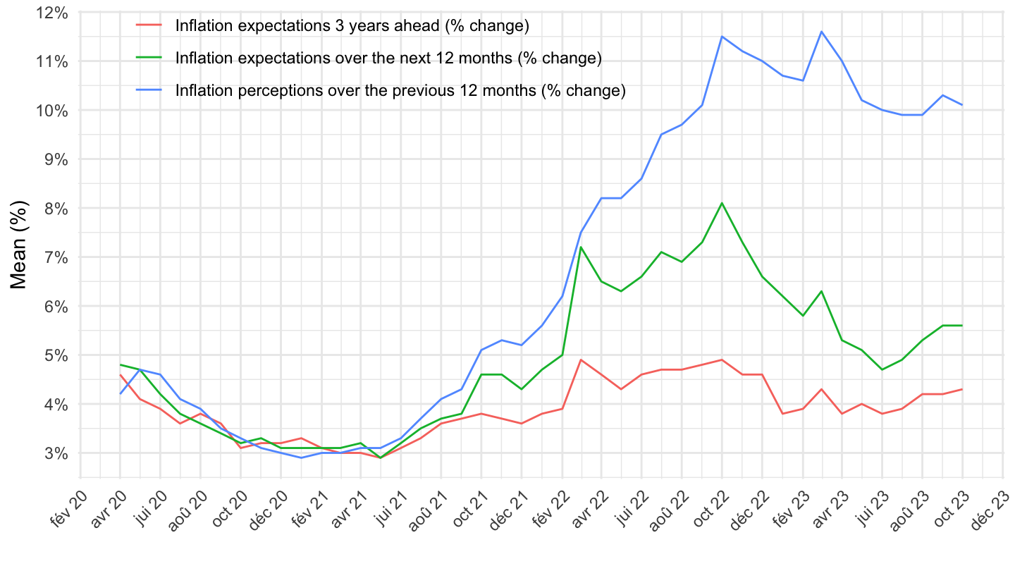
Median
Code
CES %>%
  wave_to_date %>%
  filter(Breakdown == "Wave",
         Var %in% c("c1020", "c1120", "c1220")) %>%
  transmute(date, Var_label, OBS_VALUE = Median/100) %>%
  ggplot(.) + geom_line(aes(x = date, y = OBS_VALUE, color = Var_label)) +
  theme_minimal() + xlab("") + ylab("Median (%)") +
  scale_x_date(breaks = seq.Date(as.Date("2019-12-01"), Sys.Date(), "2 months"),
               labels = date_format("%b %y")) +
  scale_y_continuous(breaks = 0.01*seq(-20, 20, 1),
                     labels = percent_format(a = 1)) +
  theme(legend.position = c(0.33, 0.90),
        axis.text.x = element_text(angle = 45, vjust = 1, hjust = 1),
        legend.title = element_blank())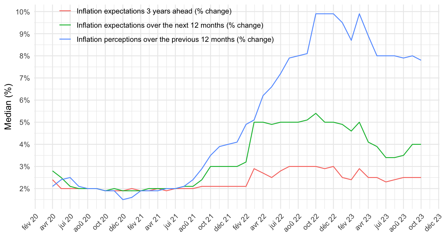
qualitative
Net percentage
Code
CES %>%
  wave_to_date %>%
  filter(Breakdown == "Wave",
         Var %in% c("c1010", "c1110", "c1210")) %>%
  transmute(date, Var_label, OBS_VALUE = Net_perc/100) %>%
  ggplot(.) + geom_line(aes(x = date, y = OBS_VALUE, color = Var_label)) +
  theme_minimal() + xlab("") + ylab("Net_perc (%)") +
  scale_x_date(breaks = seq.Date(as.Date("2019-12-01"), Sys.Date(), "2 months"),
               labels = date_format("%b %y")) +
  scale_y_continuous(breaks = 0.01*seq(-20, 100, 5),
                     labels = percent_format(a = 1)) +
  theme(legend.position = c(0.33, 0.90),
        axis.text.x = element_text(angle = 45, vjust = 1, hjust = 1),
        legend.title = element_blank())
Up
Code
CES %>%
  wave_to_date %>%
  filter(Breakdown == "Wave",
         Var %in% c("c1010", "c1110", "c1210")) %>%
  transmute(date, Var_label, OBS_VALUE = Net_perc/100) %>%
  ggplot(.) + geom_line(aes(x = date, y = OBS_VALUE, color = Var_label)) +
  theme_minimal() + xlab("") + ylab("Up (%)") +
  scale_x_date(breaks = seq.Date(as.Date("2019-12-01"), Sys.Date(), "2 months"),
               labels = date_format("%b %y")) +
  scale_y_continuous(breaks = 0.01*seq(-20, 100, 5),
                     labels = percent_format(a = 1)) +
  theme(legend.position = c(0.33, 0.90),
        axis.text.x = element_text(angle = 45, vjust = 1, hjust = 1),
        legend.title = element_blank())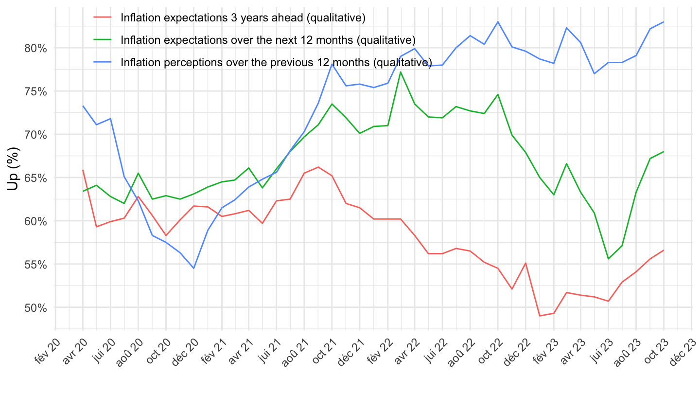
Down
Code
CES %>%
  wave_to_date %>%
  filter(Breakdown == "Wave",
         Var %in% c("c1010", "c1110", "c1210")) %>%
  transmute(date, Var_label, OBS_VALUE = Down/100) %>%
  ggplot(.) + geom_line(aes(x = date, y = OBS_VALUE, color = Var_label)) +
  theme_minimal() + xlab("") + ylab("Up (%)") +
  scale_x_date(breaks = seq.Date(as.Date("2019-12-01"), Sys.Date(), "2 months"),
               labels = date_format("%b %y")) +
  scale_y_continuous(breaks = 0.01*seq(-20, 100, 1),
                     labels = percent_format(a = 1)) +
  theme(legend.position = c(0.33, 0.90),
        axis.text.x = element_text(angle = 45, vjust = 1, hjust = 1),
        legend.title = element_blank())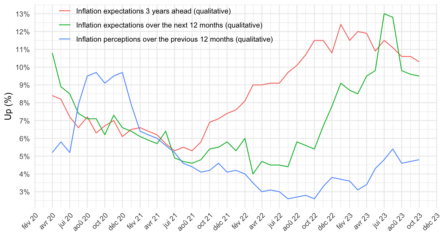
France, Germany, Italy, Spain
1-year
Mean
All
Code
CES %>%
  wave_to_date %>%
  filter(Breakdown == "Country",
         Var == "c1020") %>%
  rename(geo = Breakdown_label) %>%
  left_join(geo, by = "geo") %>%
  left_join(colors, by = c("Geo" = "country")) %>%
  mutate(OBS_VALUE = Mean/100) %>%
  rename(Ref_area = Geo) %>%
  ggplot(.) + geom_line(aes(x = date, y = OBS_VALUE, color = color)) +
  theme_minimal() + xlab("") + ylab("Inflation expectations over the next 12 months\n% change, Mean") +
  scale_x_date(breaks = seq.Date(as.Date("2019-12-01"), Sys.Date(), "2 months"),
               labels = date_format("%b %y")) +
  scale_y_continuous(breaks = 0.01*seq(-20, 20, 1),
                     labels = percent_format(a = 1)) +
  scale_color_identity() + add_flags +
  theme(legend.position = c(0.75, 0.90),
        axis.text.x = element_text(angle = 45, vjust = 1, hjust = 1),
        legend.title = element_blank())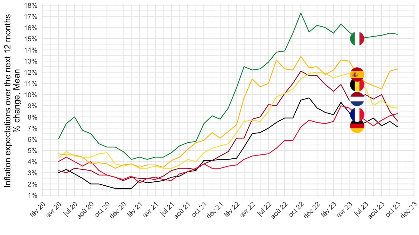
October 2021-
Code
CES %>%
  wave_to_date %>%
  filter(Breakdown == "Country",
         Var == "c1020") %>%
  rename(geo = Breakdown_label) %>%
  left_join(geo, by = "geo") %>%
  left_join(colors, by = c("Geo" = "country")) %>%
  mutate(OBS_VALUE = Mean/100) %>%
  filter(date >= as.Date("2021-10-01")) %>%
  rename(Ref_area = Geo) %>%
  ggplot(.) + geom_line(aes(x = date, y = OBS_VALUE, color = color)) +
  theme_minimal() + xlab("") + ylab("Inflation expectations over the next 12 months\n% change, Mean") +
  scale_x_date(breaks = seq.Date(as.Date("2019-12-01"), Sys.Date(), "1 month"),
               labels = date_format("%b %y")) +
  scale_y_continuous(breaks = 0.01*seq(-20, 20, 1),
                     labels = percent_format(a = 1)) +
  scale_color_identity() + add_flags +
  theme(legend.position = c(0.75, 0.90),
        axis.text.x = element_text(angle = 45, vjust = 1, hjust = 1),
        legend.title = element_blank())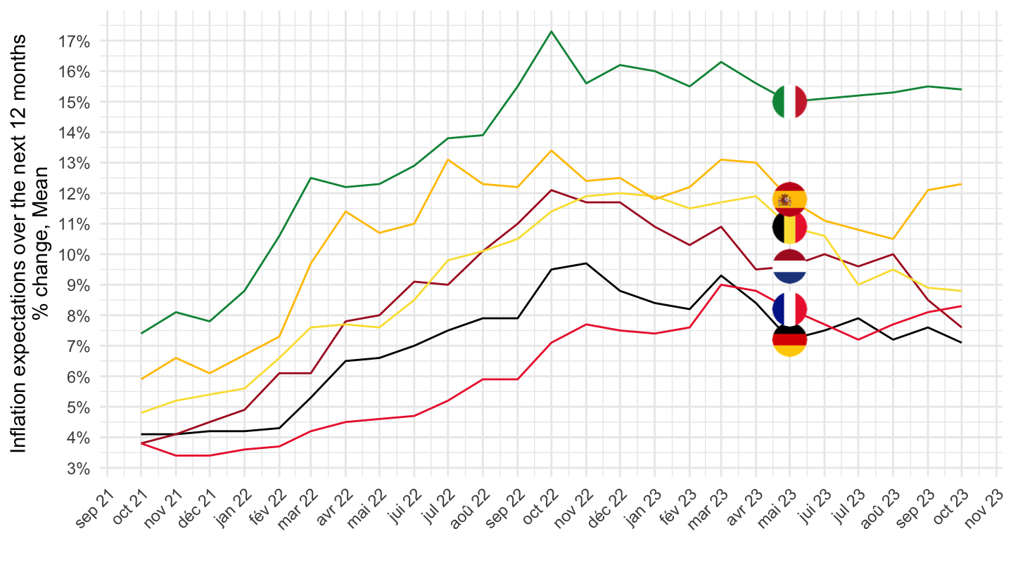
Median
All
Code
CES %>%
  wave_to_date %>%
  filter(Breakdown == "Country",
         Var == "c1020") %>%
  rename(geo = Breakdown_label) %>%
  left_join(geo, by = "geo") %>%
  left_join(colors, by = c("Geo" = "country")) %>%
  mutate(OBS_VALUE = Median/100) %>%
  rename(Ref_area = Geo) %>%
  ggplot(.) + geom_line(aes(x = date, y = OBS_VALUE, color = color)) +
  theme_minimal() + xlab("") + ylab("Inflation expectations over the next 12 months\n% change, Median") +
  scale_x_date(breaks = seq.Date(as.Date("2019-12-01"), Sys.Date(), "2 months"),
               labels = date_format("%b %y")) +
  scale_y_continuous(breaks = 0.01*seq(-20, 20, 1),
                     labels = percent_format(a = 1)) +
  scale_color_identity() + add_flags +
  theme(legend.position = c(0.75, 0.90),
        axis.text.x = element_text(angle = 45, vjust = 1, hjust = 1),
        legend.title = element_blank())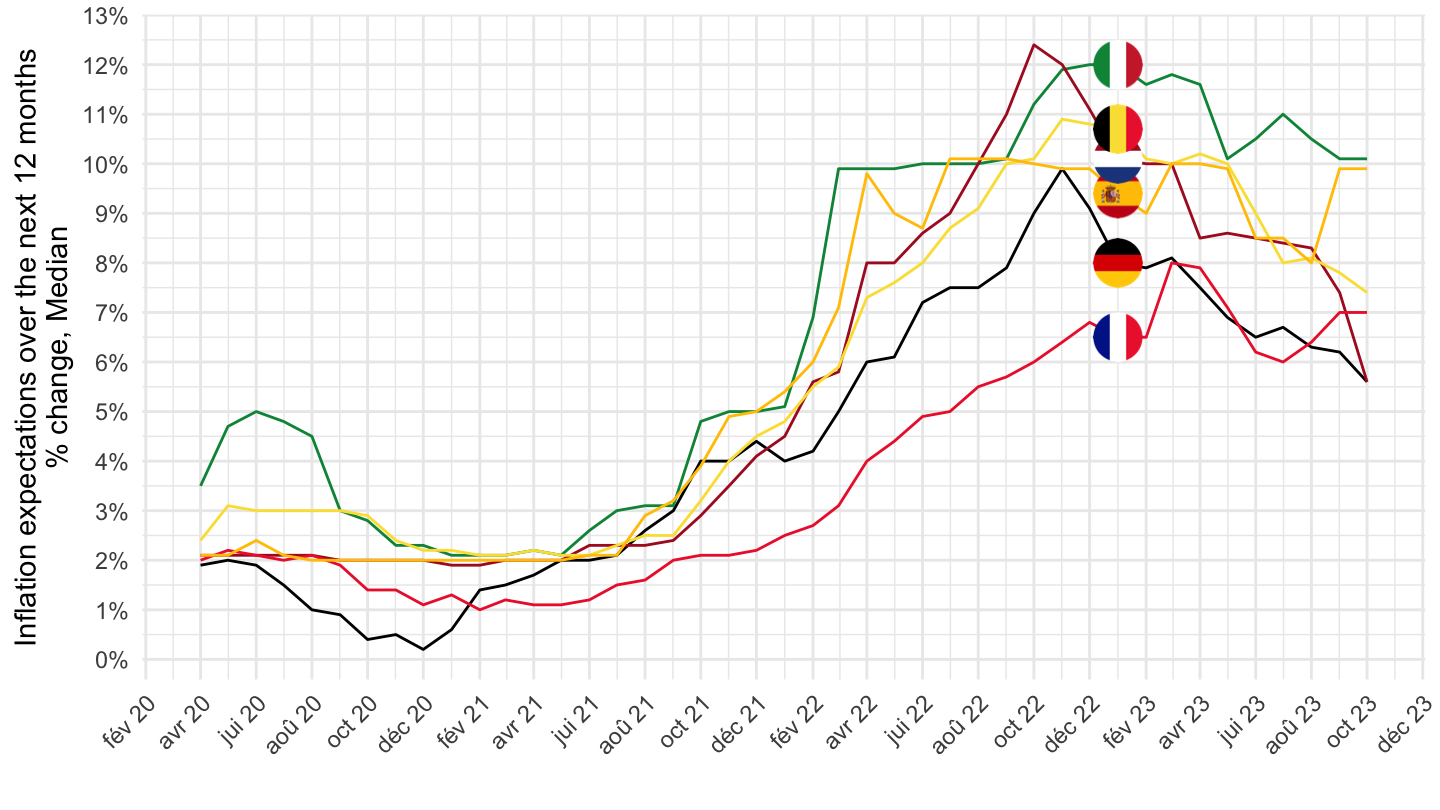
October 2021-
Code
CES %>%
  wave_to_date %>%
  filter(Breakdown == "Country",
         Var == "c1020") %>%
  rename(geo = Breakdown_label) %>%
  left_join(geo, by = "geo") %>%
  left_join(colors, by = c("Geo" = "country")) %>%
  mutate(OBS_VALUE = Median/100) %>%
  filter(date >= as.Date("2021-10-01")) %>%
  rename(Ref_area = Geo) %>%
  ggplot(.) + geom_line(aes(x = date, y = OBS_VALUE, color = color)) +
  theme_minimal() + xlab("") + ylab("Inflation expectations over the next 12 months\n% change, Median") +
  scale_x_date(breaks = seq.Date(as.Date("2019-12-01"), Sys.Date(), "1 month"),
               labels = date_format("%b %y")) +
  scale_y_continuous(breaks = 0.01*seq(-20, 20, 1),
                     labels = percent_format(a = 1)) +
  scale_color_identity() + add_flags +
  theme(legend.position = c(0.75, 0.90),
        axis.text.x = element_text(angle = 45, vjust = 1, hjust = 1),
        legend.title = element_blank())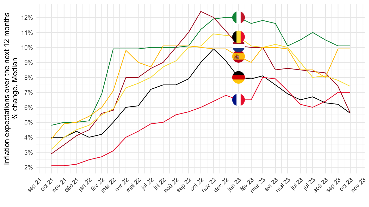
3-year
Mean
All
Code
CES %>%
  wave_to_date %>%
  filter(Breakdown == "Country",
         Var == "c1220") %>%
  rename(geo = Breakdown_label) %>%
  left_join(geo, by = "geo") %>%
  left_join(colors, by = c("Geo" = "country")) %>%
  mutate(OBS_VALUE = Mean/100) %>%
  rename(Ref_area = Geo) %>%
  ggplot(.) + geom_line(aes(x = date, y = OBS_VALUE, color = color)) +
  theme_minimal() + xlab("") + ylab("Inflation expectations 3 years ahead\n% change, Mean") +
  scale_x_date(breaks = seq.Date(as.Date("2019-12-01"), Sys.Date(), "2 months"),
               labels = date_format("%b %y")) +
  scale_y_continuous(breaks = 0.01*seq(-20, 20, 1),
                     labels = percent_format(a = 1)) +
  scale_color_identity() + add_flags +
  theme(legend.position = c(0.75, 0.90),
        axis.text.x = element_text(angle = 45, vjust = 1, hjust = 1),
        legend.title = element_blank())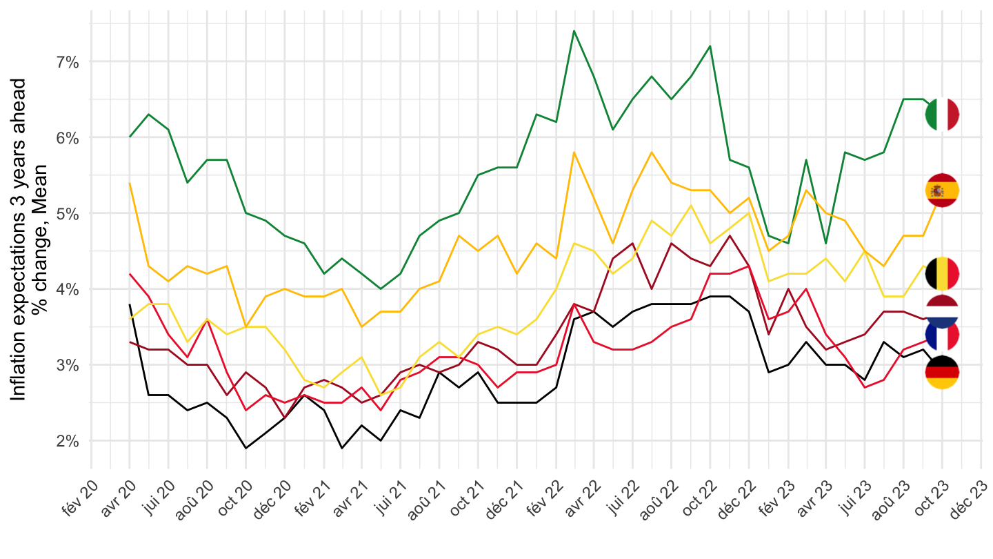
October 2021-
Code
CES %>%
  wave_to_date %>%
  filter(Breakdown == "Country",
         Var == "c1220",
         date >= as.Date("2021-10-01")) %>%
  rename(geo = Breakdown_label) %>%
  left_join(geo, by = "geo") %>%
  left_join(colors, by = c("Geo" = "country")) %>%
  mutate(OBS_VALUE = Mean/100) %>%
  rename(Ref_area = Geo) %>%
  ggplot(.) + geom_line(aes(x = date, y = OBS_VALUE, color = color)) +
  theme_minimal() + xlab("") + ylab("Inflation expectations 3 years ahead\n% change, Mean") +
  scale_x_date(breaks = seq.Date(as.Date("2019-12-01"), Sys.Date(), "1 month"),
               labels = date_format("%b %y")) +
  scale_y_continuous(breaks = 0.01*seq(-20, 20, 1),
                     labels = percent_format(a = 1)) +
  scale_color_identity() + add_flags +
  theme(legend.position = c(0.75, 0.90),
        axis.text.x = element_text(angle = 45, vjust = 1, hjust = 1),
        legend.title = element_blank())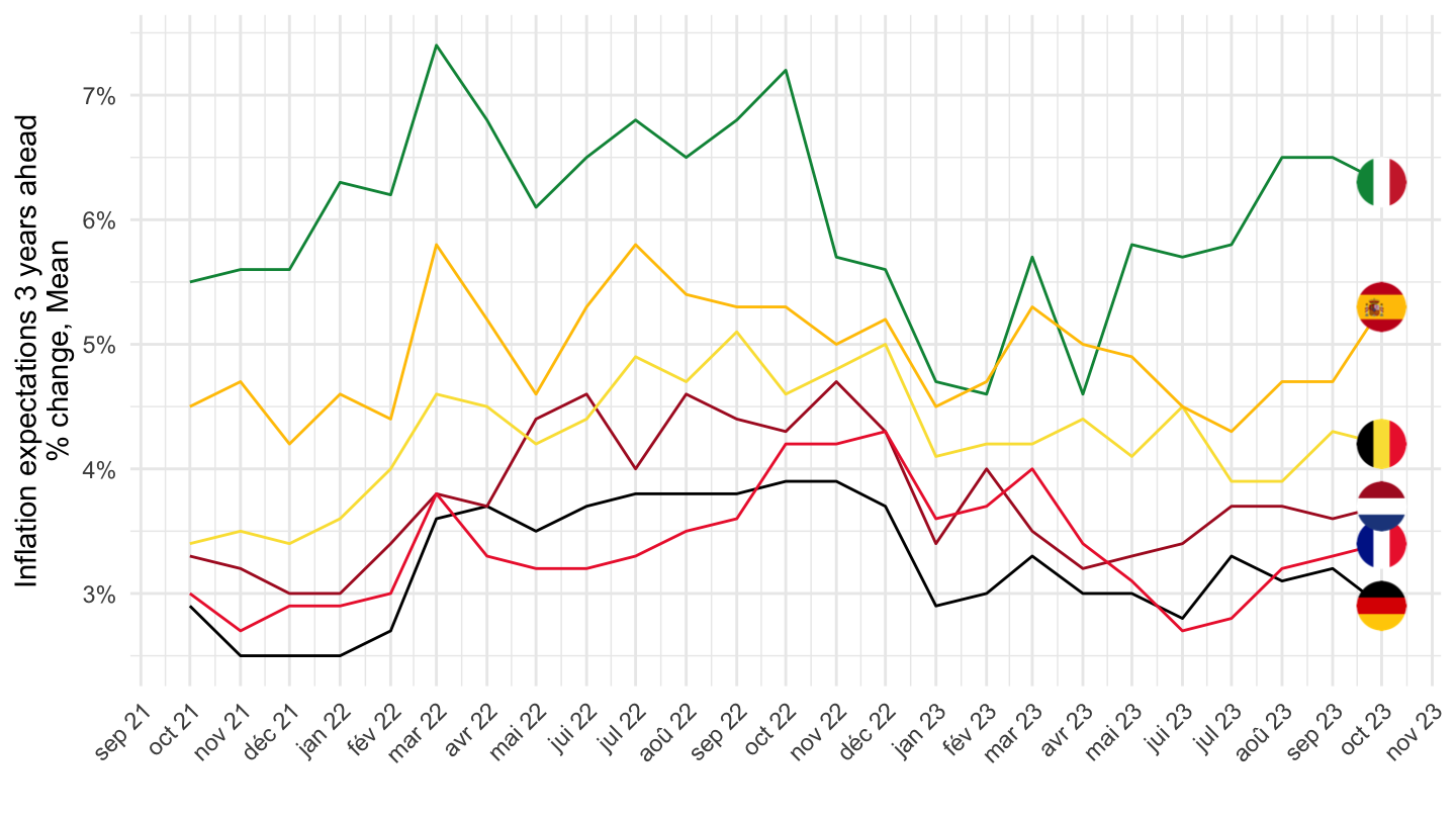
Median
All
Code
CES %>%
  wave_to_date %>%
  filter(Breakdown == "Country",
         Var == "c1220") %>%
  rename(geo = Breakdown_label) %>%
  left_join(geo, by = "geo") %>%
  left_join(colors, by = c("Geo" = "country")) %>%
  mutate(OBS_VALUE = Median/100) %>%
  rename(Ref_area = Geo) %>%
  ggplot(.) + geom_line(aes(x = date, y = OBS_VALUE, color = color)) +
  theme_minimal() + xlab("") + ylab("Inflation expectations 3 years ahead\n% change, Median") +
  scale_x_date(breaks = seq.Date(as.Date("2019-12-01"), Sys.Date(), "2 months"),
               labels = date_format("%b %y")) +
  scale_y_continuous(breaks = 0.01*seq(-20, 20, .2),
                     labels = percent_format(a = .1)) +
  scale_color_identity() + add_flags +
  theme(legend.position = c(0.75, 0.90),
        axis.text.x = element_text(angle = 45, vjust = 1, hjust = 1),
        legend.title = element_blank())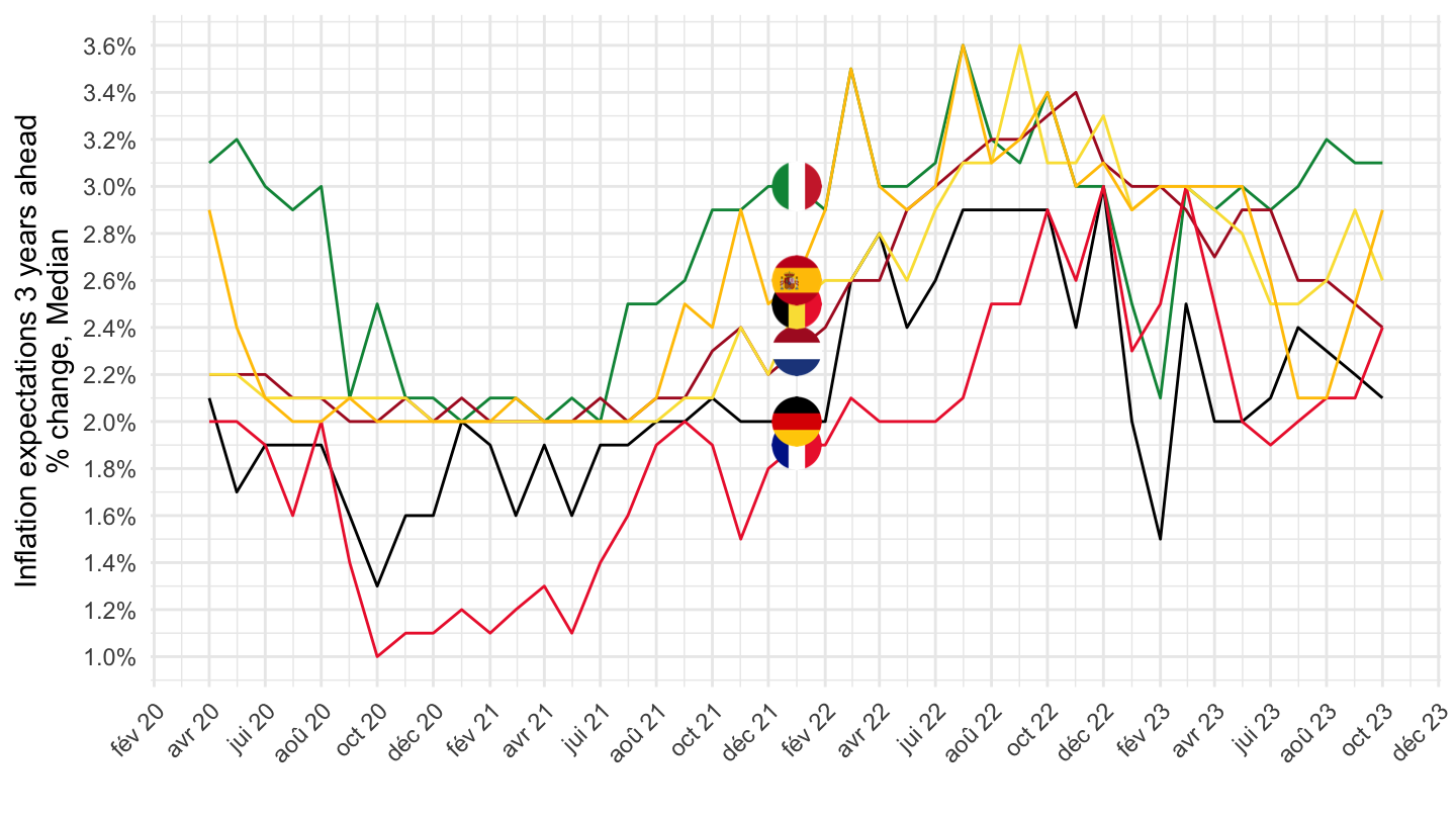
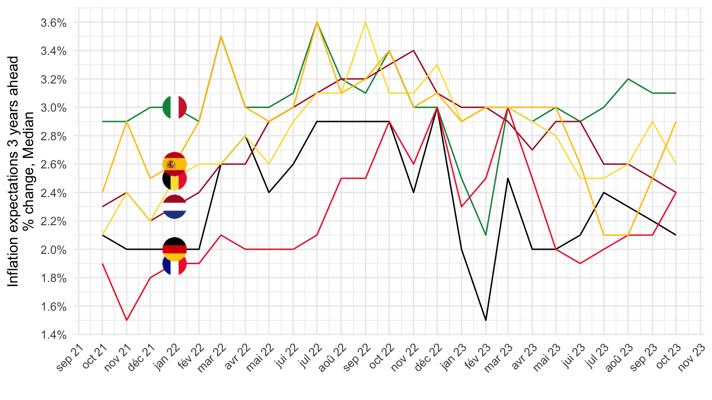
October 2021-
Code
CES %>%
  wave_to_date %>%
  filter(Breakdown == "Country",
         Var == "c1220",
         date >= as.Date("2021-10-01")) %>%
  rename(geo = Breakdown_label) %>%
  left_join(geo, by = "geo") %>%
  left_join(colors, by = c("Geo" = "country")) %>%
  mutate(OBS_VALUE = Median/100) %>%
  rename(Ref_area = Geo) %>%
  ggplot(.) + geom_line(aes(x = date, y = OBS_VALUE, color = color)) +
  theme_minimal() + xlab("") + ylab("Inflation expectations 3 years ahead\n% change, Median") +
  scale_x_date(breaks = seq.Date(as.Date("2019-12-01"), Sys.Date(), "1 month"),
               labels = date_format("%b %y")) +
  scale_y_continuous(breaks = 0.01*seq(-20, 20, .2),
                     labels = percent_format(a = .1)) +
  scale_color_identity() + add_flags +
  theme(legend.position = c(0.75, 0.90),
        axis.text.x = element_text(angle = 45, vjust = 1, hjust = 1),
        legend.title = element_blank())