| source | dataset | Title | .html | .rData |
|---|---|---|---|---|
| oecd | SNA_TABLE1 | Gross domestic product (GDP) | 2026-07-24 | 2025-05-24 |
Gross domestic product (GDP)
Data - OECD
Info
Data on main macro
| source | dataset | Title | .html | .rData |
|---|---|---|---|---|
| oecd | SNA_TABLE1 | Gross domestic product (GDP) | 2026-07-24 | 2025-05-24 |
| eurostat | nama_10_a10 | Gross value added and income by A*10 industry breakdowns | 2026-07-24 | 2026-07-23 |
| eurostat | nama_10_a10_e | Employment by A*10 industry breakdowns | 2026-07-24 | 2026-07-23 |
| eurostat | nama_10_gdp | GDP and main components (output, expenditure and income) | 2026-07-24 | 2026-07-23 |
| eurostat | nama_10_lp_ulc | Labour productivity and unit labour costs | 2026-07-22 | 2026-07-23 |
| eurostat | namq_10_a10 | Gross value added and income A*10 industry breakdowns | 2026-07-25 | 2026-07-24 |
| eurostat | namq_10_a10_e | Employment A*10 industry breakdowns | 2026-07-24 | 2026-07-24 |
| eurostat | namq_10_gdp | GDP and main components (output, expenditure and income) | 2026-07-24 | 2026-07-23 |
| eurostat | namq_10_lp_ulc | Labour productivity and unit labour costs | 2026-07-24 | 2026-07-24 |
| eurostat | namq_10_pc | Main GDP aggregates per capita | 2026-07-24 | 2026-07-24 |
| eurostat | nasa_10_nf_tr | Non-financial transactions | 2026-07-25 | 2026-07-23 |
| eurostat | nasq_10_nf_tr | Non-financial transactions | 2026-07-25 | 2026-07-23 |
| fred | gdp | Gross Domestic Product | 2026-07-24 | 2026-07-24 |
| oecd | QNA | Quarterly National Accounts | 2026-07-24 | 2026-07-24 |
| oecd | SNA_TABLE14A | Non-financial accounts by sectors | 2026-07-24 | 2024-06-30 |
| oecd | SNA_TABLE2 | Disposable income and net lending - net borrowing | 2024-07-01 | 2024-04-11 |
| oecd | SNA_TABLE6A | Value added and its components by activity, ISIC rev4 | 2024-07-01 | 2024-06-30 |
| wdi | NE.RSB.GNFS.ZS | External balance on goods and services (% of GDP) | 2026-07-25 | 2026-07-24 |
| wdi | NY.GDP.MKTP.CD | GDP (current USD) | 2026-07-25 | 2026-07-24 |
| wdi | NY.GDP.MKTP.PP.CD | GDP, PPP (current international D) | 2026-07-25 | 2026-07-24 |
| wdi | NY.GDP.PCAP.CD | GDP per capita (current USD) | 2026-07-25 | 2026-07-24 |
| wdi | NY.GDP.PCAP.KD | GDP per capita (constant 2015 USD) | 2026-07-25 | 2026-07-24 |
| wdi | NY.GDP.PCAP.PP.CD | GDP per capita, PPP (current international D) | 2026-07-25 | 2026-07-24 |
| wdi | NY.GDP.PCAP.PP.KD | GDP per capita, PPP (constant 2011 international D) | 2026-07-25 | 2026-07-24 |
Data on industry
| source | dataset | Title | .html | .rData |
|---|---|---|---|---|
| ec | INDUSTRY | Industry (sector data) | 2026-07-24 | 2026-07-24 |
| eurostat | ei_isin_m | Industry - monthly data - index (2015 = 100) (NACE Rev. 2) - ei_isin_m | 2026-07-22 | 2026-07-23 |
| eurostat | htec_trd_group4 | High-tech trade by high-tech group of products in million euro (from 2007, SITC Rev. 4) | 2026-07-22 | 2026-07-23 |
| eurostat | nama_10_a64 | National accounts aggregates by industry (up to NACE A*64) | 2026-07-17 | 2026-07-23 |
| eurostat | nama_10_a64_e | National accounts employment data by industry (up to NACE A*64) | 2026-07-24 | 2026-07-24 |
| eurostat | namq_10_a10_e | Employment A*10 industry breakdowns | 2026-07-24 | 2026-07-24 |
| eurostat | road_eqr_carmot | New registrations of passenger cars by type of motor energy and engine size - road_eqr_carmot | 2026-07-24 | 2026-07-23 |
| eurostat | sts_inpp_m | Producer prices in industry, total - monthly data | 2026-07-21 | 2026-07-24 |
| eurostat | sts_inppd_m | Producer prices in industry, domestic market - monthly data | 2026-07-21 | 2026-07-24 |
| eurostat | sts_inpr_m | Production in industry - monthly data | 2026-07-21 | 2026-07-23 |
| eurostat | sts_intvnd_m | Turnover in industry, non domestic market - monthly data - sts_intvnd_m | 2026-07-24 | 2026-07-24 |
| fred | industry | Manufacturing, Industry | 2026-07-24 | 2026-07-24 |
| oecd | ALFS_EMP | Employment by activities and status (ALFS) | 2026-07-24 | 2025-05-24 |
| oecd | BERD_MA_SOF | Business enterprise R&D expenditure by main activity (focussed) and source of funds | 2026-07-24 | 2023-09-09 |
| oecd | GBARD_NABS2007 | Government budget allocations for R and D | 2024-04-16 | 2023-11-22 |
| oecd | MEI_REAL | Production and Sales (MEI) | 2024-05-12 | 2025-05-24 |
| oecd | MSTI_PUB | Main Science and Technology Indicators | 2024-09-15 | 2025-05-24 |
| oecd | SNA_TABLE4 | PPPs and exchange rates | 2024-09-15 | 2025-05-24 |
| wdi | NV.IND.EMPL.KD | Industry, value added per worker (constant 2010 USD) | 2026-07-25 | 2026-07-24 |
| wdi | NV.IND.MANF.CD | Manufacturing, value added (current USD) | 2026-07-25 | 2026-07-24 |
| wdi | NV.IND.MANF.ZS | Manufacturing, value added (% of GDP) | 2026-07-25 | 2026-07-24 |
| wdi | NV.IND.TOTL.KD | Industry (including construction), value added (constant 2015 USD) - NV.IND.TOTL.KD | 2026-07-25 | 2026-07-24 |
| wdi | NV.IND.TOTL.ZS | Industry, value added (including construction) (% of GDP) | 2026-07-25 | 2026-07-24 |
| wdi | SL.IND.EMPL.ZS | Employment in industry (% of total employment) | 2026-07-25 | 2026-07-24 |
| wdi | TX.VAL.MRCH.CD.WT | Merchandise exports (current USD) | 2026-07-25 | 2026-07-24 |
LAST_COMPILE
| LAST_COMPILE |
|---|
| 2026-07-26 |
Last
| obsTime | Nobs |
|---|---|
| 2018 | 38400 |
Layout - By country
- OECD Website. html
Nobs - Javascript
Code
SNA_TABLE1 %>%
  left_join(SNA_TABLE1_var$TRANSACT, by = "TRANSACT") %>%
  left_join(SNA_TABLE1_var$MEASURE, by = "MEASURE") %>%
  group_by(TRANSACT, Transact, MEASURE, Measure) %>%
  summarise(nobs = n()) %>%
  arrange(-nobs) %>%
  {if (is_html_output()) datatable(., filter = 'top', rownames = F) else .}
TRANSACT
Code
SNA_TABLE1 %>%
  left_join(SNA_TABLE1_var$TRANSACT, by = "TRANSACT") %>%
  group_by(TRANSACT, Transact) %>%
  summarise(Nobs = n()) %>%
  arrange(-Nobs) %>%
  print_table_conditional()
MEASURE
Code
SNA_TABLE1 %>%
  left_join(SNA_TABLE1_var$MEASURE, by = "MEASURE") %>%
  group_by(MEASURE, Measure) %>%
  summarise(Nobs = n()) %>%
print_table_conditional()| MEASURE | Measure | Nobs |
|---|---|---|
| C | Current prices | 146635 |
| CPC | Current prices, current PPPs | 61110 |
| CXC | Current prices, current exchange rates | 146628 |
| DOB | Deflator | 79777 |
| G | Growth rate | 70321 |
| HCPC | Per head, current prices, current PPPs | 6423 |
| HCPIXOE | Per head, index using current prices and current PPPs | 2979 |
| HCXC | Per head, current prices, current exchange rates | 6631 |
| HVPIXOE | Per head, index using the price levels and PPPs of 2010 | 2960 |
| HVPVOB | Per head, constant prices, constant PPPs, OECD base year | 6344 |
| HVXVOB | Per head, constant prices, constant exchange rates, OECD base year | 6368 |
| PVP | Previous year prices and previous year PPPs | 45839 |
| V | Constant prices, national base year | 82479 |
| VIXOB | Volume index | 80700 |
| VOB | Constant prices, OECD base year | 82406 |
| VP | Constant prices, previous year prices | 65225 |
| VPCOB | Current prices, constant PPPs, OECD base year | 60626 |
| VPVOB | Constant prices, constant PPPs, OECD base year | 53413 |
| VXCOB | Current prices, constant exchange rates, OECD base year | 145416 |
| VXVOB | Constant prices, constant exchange rates, OECD base year | 81686 |
| XVP | Previous year prices and previous year exchange rates | 69473 |
| NA | NA | 93899 |
LOCATION
Code
SNA_TABLE1 %>%
  left_join(SNA_TABLE1_var$LOCATION, by = "LOCATION") %>%
  group_by(LOCATION, Location) %>%
  summarise(Nobs = n()) %>%
  arrange(-Nobs) %>%
  mutate(Flag = gsub(" ", "-", str_to_lower(gsub(" ", "-", Location))),
         Flag = paste0('<img src="../../icon/flag/vsmall/', Flag, '.png" alt="Flag">')) %>%
  select(Flag, everything()) %>%
  {if (is_html_output()) datatable(., filter = 'top', rownames = F, escape = F) else .}
Goods Net Exports
NX, Total, Goods, Services
Code
SNA_TABLE1 %>%
  filter(obsTime == "2018",
         MEASURE == "C",
         TRANSACT %in% c("B1_GE", "P61", "P71", "P62", "P72", "P6", "P7")) %>%
  left_join(SNA_TABLE1_var$LOCATION, by = "LOCATION") %>%
  group_by(Location) %>%
  mutate(obsValue = 100*obsValue / obsValue[TRANSACT == "B1_GE"]) %>%
  filter(TRANSACT != "B1_GE") %>%
  select(LOCATION, Location, TRANSACT, obsValue) %>%
  na.omit %>%
  spread(TRANSACT, obsValue) %>%
  mutate(NX = P6 - P7,
         `Goods NX` = P61 - P71,
         `Services NX` = P62 - P72) %>%
  select(LOCATION, Location, NX, `Goods NX`, `Services NX`) %>%
  arrange(-`Goods NX`) %>%
  mutate_at(vars(-1, -2), funs(ifelse(is.na(.), NA, paste0(round(., 1), "%")))) %>%
  mutate(Flag = gsub(" ", "-", str_to_lower(gsub(" ", "-", Location))),
         Flag = paste0('<img src="../../icon/flag/vsmall/', Flag, '.png" alt="Flag">')) %>%
  select(Flag, everything()) %>%
  {if (is_html_output()) datatable(., filter = 'top', rownames = F, escape = F) else .}
France, Germany, United Kingdom
Code
SNA_TABLE1 %>%
  filter(LOCATION %in% c("DEU", "FRA", "GBR"),
         MEASURE == "C",
         TRANSACT %in% c("B1_GE", "P61", "P71")) %>%
  year_to_date %>%
  left_join(SNA_TABLE1_var$LOCATION, by = "LOCATION") %>%
  select(date, Location, TRANSACT, obsValue) %>%
  spread(TRANSACT, obsValue) %>%
  mutate(obsValue = (P61 - P71)/B1_GE) %>%
  left_join(colors, by = c("Location" = "country")) %>%
  ggplot() + theme_minimal() + ylab("Goods Net Exports (% of GDP)") + xlab("") +
  geom_line(aes(x = date, y = obsValue, color = color)) +
  scale_color_identity() + add_3flags +
  scale_x_date(breaks = seq(1920, 2100, 10) %>% paste0("-01-01") %>% as.Date,
               labels = date_format("%Y")) +
  scale_y_continuous(breaks = 0.01*seq(-10, 100, 1),
                     labels = scales::percent_format(accuracy = 1)) +
  geom_hline(yintercept = 0, linetype = "dashed")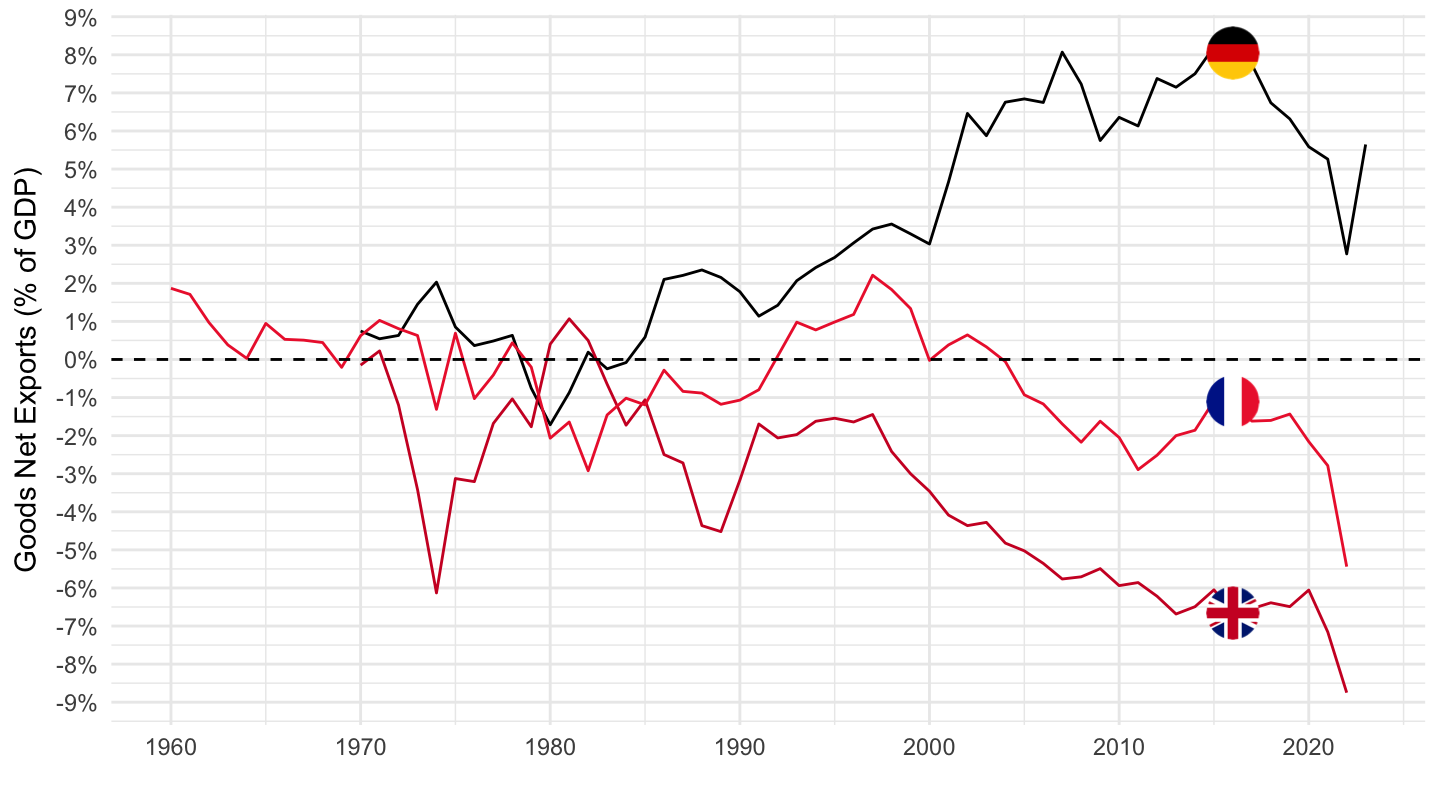
Italy, Portugal, Spain
Code
SNA_TABLE1 %>%
  filter(LOCATION %in% c("ITA", "PRT", "ESP"),
         MEASURE == "C",
         TRANSACT %in% c("B1_GE", "P61", "P71")) %>%
  year_to_date %>%
  left_join(SNA_TABLE1_var$LOCATION, by = "LOCATION") %>%
  select(date, Location, TRANSACT, obsValue) %>%
  spread(TRANSACT, obsValue) %>%
  mutate(obsValue = (P61 - P71)/B1_GE) %>%
  left_join(colors, by = c("Location" = "country")) %>%
  ggplot() + theme_minimal() + ylab("Goods Net Exports (% of GDP)") + xlab("") +
  geom_line(aes(x = date, y = obsValue, color = color)) +
  scale_color_identity() + add_3flags +
  scale_x_date(breaks = seq(1920, 2100, 10) %>% paste0("-01-01") %>% as.Date,
               labels = date_format("%Y")) +
  scale_y_continuous(breaks = 0.01*seq(-30, 100, 1),
                     labels = scales::percent_format(accuracy = 1)) +
  geom_hline(yintercept = 0, linetype = "dashed")
Netherlands, Russia, Switzerland
Code
SNA_TABLE1 %>%
  filter(LOCATION %in% c("RUS", "NLD", "CHE"),
         MEASURE == "C",
         TRANSACT %in% c("B1_GE", "P61", "P71")) %>%
  year_to_date %>%
  left_join(SNA_TABLE1_var$LOCATION, by = "LOCATION") %>%
  select(date, Location, TRANSACT, obsValue) %>%
  spread(TRANSACT, obsValue) %>%
  mutate(obsValue = (P61 - P71)/B1_GE) %>%
  left_join(colors, by = c("Location" = "country")) %>%
  ggplot() + theme_minimal() + ylab("Goods Net Exports (% of GDP)") + xlab("") +
  geom_line(aes(x = date, y = obsValue, color = color)) +
  scale_color_identity() + add_3flags +
  scale_x_date(breaks = seq(1920, 2100, 10) %>% paste0("-01-01") %>% as.Date,
               labels = date_format("%Y")) +
  scale_y_continuous(breaks = 0.01*seq(-10, 100, 1),
                     labels = scales::percent_format(accuracy = 1)) +
  geom_hline(yintercept = 0, linetype = "dashed")
Industry/ Manufacturing Decline and Trade Deficits
Industry
Code
SNA_TABLE1 %>%
  mutate(date = paste0(obsTime, "-12-31") %>% as.Date) %>%
  filter(MEASURE == "C",
         TRANSACT %in% c("B1_GE", "B1GVB_E", "B11", "P61", "P71"),
         date >= as.Date("2016-01-01"),
         date <= as.Date("2020-01-01")) %>%
  select(date, LOCATION, TRANSACT, obsValue) %>%
  spread(TRANSACT, obsValue) %>%
  group_by(LOCATION) %>%
  summarise(NX_mean = mean((P61-P71) / B1_GE, na.rm = T),
            IND_mean = mean(B1GVB_E / B1_GE, na.rm = T)) %>%
  left_join(SNA_TABLE1_var$LOCATION, by = "LOCATION") %>%
  ggplot(.) + theme_minimal() + geom_point(aes(x = NX_mean, y = IND_mean)) +
  xlab("Goods Trade Balance 2015-2020 (% of GDP)") +
  ylab("Industry VA 2015-2020 (% of GDP)") +
  scale_x_continuous(breaks = 0.01*seq(-100, 100, 5),
                     labels = percent_format(accuracy = 1)) +
  scale_y_continuous(breaks = 0.01*seq(-100, 100, 5),
                     labels = percent_format(accuracy = 1)) +
  stat_smooth(aes(x = NX_mean, y = IND_mean),
              linetype = 2, method = "lm", color = viridis(3)[2]) +
  geom_text_repel(aes(x = NX_mean, y = IND_mean, label = Location), vjust = 0)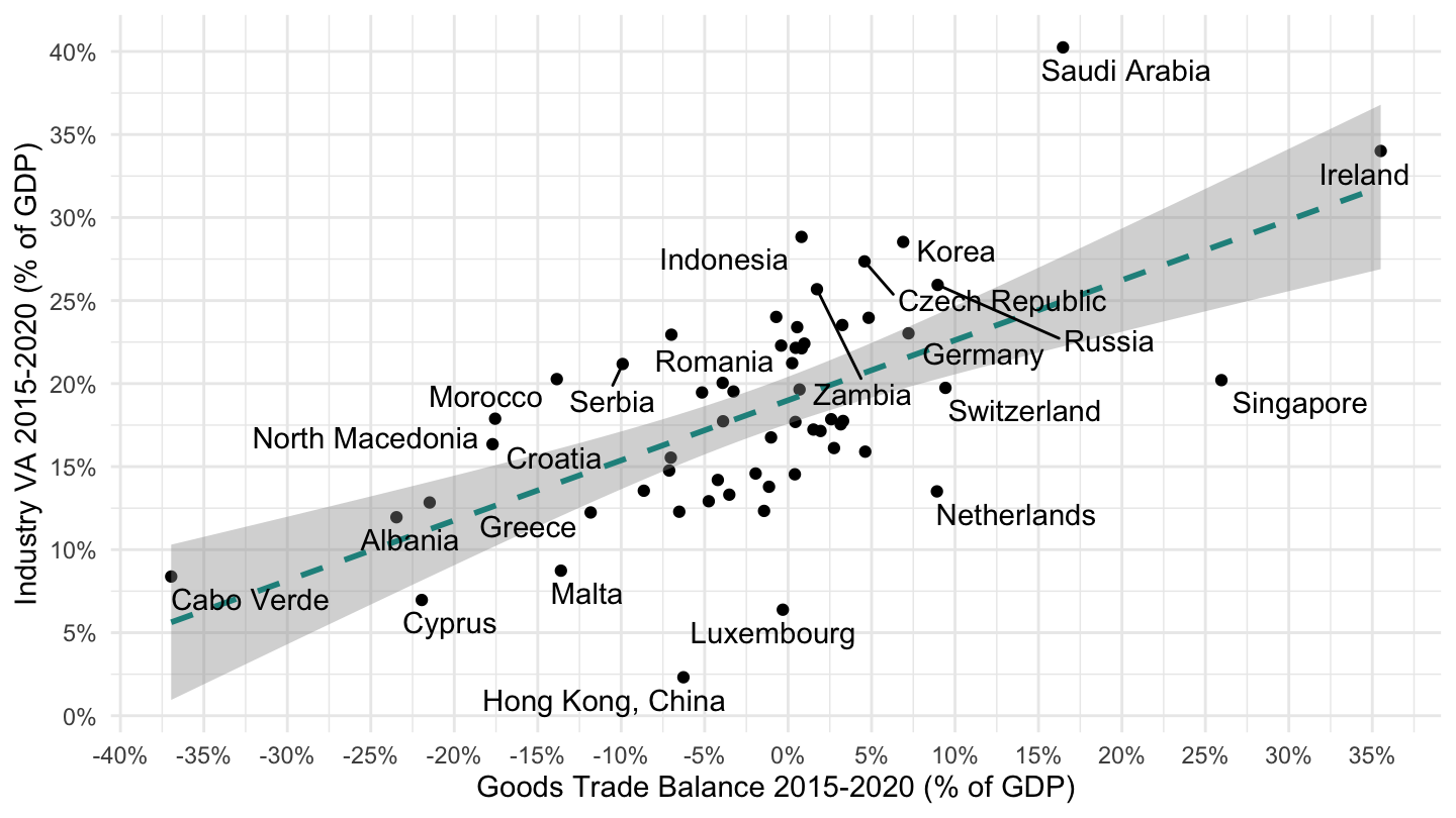
Industry
Code
SNA_TABLE1 %>%
  filter(MEASURE == "C",
         TRANSACT %in% c("B1_GE", "B1GVC", "B11", "P61", "P71")) %>%
  year_to_date %>%
  filter(date >= as.Date("2000-01-01"),
         date <= as.Date("2004-01-01")) %>%
  select(date, LOCATION, TRANSACT, obsValue) %>%
  spread(TRANSACT, obsValue) %>%
  mutate(IND = B1GVC / B1_GE,
         NX = (P61-P71) / B1_GE) %>%
  group_by(LOCATION) %>%
  summarise(NX_mean = mean(NX, na.rm = T),
            IND_mean = mean(IND, na.rm = T)) %>%
  left_join(SNA_TABLE1_var$LOCATION, by = "LOCATION") %>%
  lm(IND_mean ~ NX_mean, data = .) %>%
  summary
#
# Call:
# lm(formula = IND_mean ~ NX_mean, data = .)
#
# Residuals:
# Min 1Q Median 3Q Max
# -0.144795 -0.028173 0.001434 0.023485 0.090271
#
# Coefficients:
# Estimate Std. Error t value Pr(>|t|)
# (Intercept) 0.162048 0.007204 22.494 <2e-16 ***
# NX_mean 0.141768 0.065857 2.153 0.0366 *
# ---
# Signif. codes: 0 '***' 0.001 '**' 0.01 '*' 0.05 '.' 0.1 ' ' 1
#
# Residual standard error: 0.04696 on 46 degrees of freedom
# (10 observations effacées parce que manquantes)
# Multiple R-squared: 0.09152, Adjusted R-squared: 0.07177
# F-statistic: 4.634 on 1 and 46 DF, p-value: 0.03662Code
SNA_TABLE1 %>%
  mutate(date = paste0(obsTime, "-12-31") %>% as.Date) %>%
  filter(MEASURE == "C",
         TRANSACT %in% c("B1_GE", "B1GVB_E", "B11", "P61", "P71"),
         date >= as.Date("2016-01-01"),
         date <= as.Date("2020-01-01"),
         LOCATION != "IRL") %>%
  select(date, LOCATION, TRANSACT, obsValue) %>%
  spread(TRANSACT, obsValue) %>%
  group_by(LOCATION) %>%
  summarise(NX_mean = mean((P61-P71) / B1_GE, na.rm = T),
            IND_mean = mean(B1GVB_E / B1_GE, na.rm = T)) %>%
  left_join(SNA_TABLE1_var$LOCATION, by = "LOCATION") %>%
  ggplot(.) + theme_minimal() + geom_point(aes(x = NX_mean, y = IND_mean)) +
  xlab("Goods Trade Balance 2015-2020 (% of GDP)") +
  ylab("Industry VA 2015-2020 (% of GDP)") +
  scale_x_continuous(breaks = 0.01*seq(-100, 100, 5),
                     labels = percent_format(accuracy = 1)) +
  scale_y_continuous(breaks = 0.01*seq(-100, 100, 5),
                     labels = percent_format(accuracy = 1)) +
  stat_smooth(aes(x = NX_mean, y = IND_mean),
              linetype = 2, method = "lm", color = viridis(3)[2]) +
  geom_text_repel(aes(x = NX_mean, y = IND_mean, label = Location), vjust = 0)
Code
var1 <- SNA_TABLE1 %>%
  mutate(date = paste0(obsTime, "-12-31") %>% as.Date) %>%
  filter(MEASURE == "C",
         TRANSACT %in% c("B1_GE", "B1GVB_E", "B11", "P61", "P71"),
         date >= as.Date("2000-01-01"),
         date <= as.Date("2018-01-01"),
         LOCATION != "IRL") %>%
  select(date, LOCATION, TRANSACT, obsValue) %>%
  spread(TRANSACT, obsValue) %>%
  group_by(LOCATION) %>%
  summarise(NX_mean = mean((P61-P71) / B1_GE, na.rm = T),
            IND_mean = mean(B1GVB_E / B1_GE, na.rm = T))

var2 <- SNA_TABLE1 %>%
  mutate(date = paste0(obsTime, "-12-31") %>% as.Date) %>%
  filter(MEASURE == "C",
         TRANSACT %in% c("B1_GE", "B1GVB_E"),
         date %in% c(as.Date("2018-12-31"), as.Date("2000-12-31")),
         LOCATION != "IRL") %>%
  select(date, LOCATION, TRANSACT, obsValue) %>%
  spread(TRANSACT, obsValue) %>%
  mutate(B1GVB_E_share = B1GVB_E/B1_GE) %>%
  group_by(LOCATION) %>%
  filter(n() == 2) %>%
  summarise(D1_B1GVB_E_share = B1GVB_E_share[date == as.Date("2018-12-31")]
            - B1GVB_E_share[date == as.Date("2000-12-31")])

var1 %>%
  inner_join(var2, by = "LOCATION") %>%
  left_join(SNA_TABLE1_var$LOCATION, by = "LOCATION") %>%
  ggplot(.) + theme_minimal() + geom_point(aes(x = NX_mean, y = D1_B1GVB_E_share)) +
  xlab("Goods Trade Balance 2000-2018 (% of GDP)") +
  ylab("Industry VA 2018 (% of GDP)") +
  scale_x_continuous(breaks = 0.01*seq(-100, 100, 5),
                     labels = percent_format(accuracy = 1)) +
  scale_y_continuous(breaks = 0.01*seq(-100, 100, 5),
                     labels = percent_format(accuracy = 1)) +
  stat_smooth(aes(x = NX_mean, y = D1_B1GVB_E_share),
              linetype = 2, method = "lm", color = viridis(3)[2]) +
  geom_text_repel(aes(x = NX_mean, y = D1_B1GVB_E_share, label = LOCATION), vjust = 0)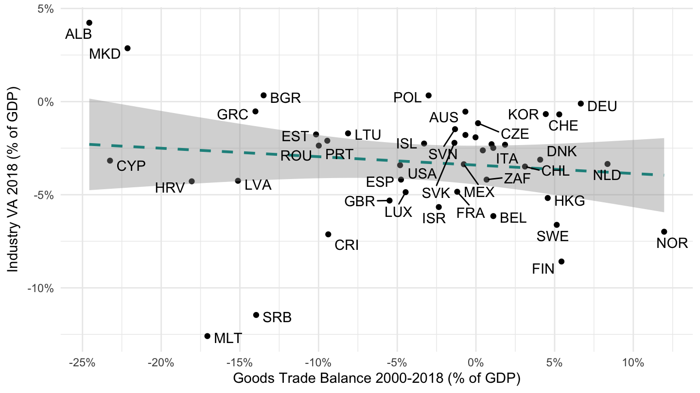
Industry (without Ireland)
Code
SNA_TABLE1 %>%
  filter(MEASURE == "C",
         TRANSACT %in% c("B1_GE", "B1GVB_E", "B11", "P61", "P71"),
         !(LOCATION == "IRL")) %>%
  year_to_date %>%
  filter(date >= as.Date("2016-01-01"),
         date <= as.Date("2020-01-01")) %>%
  select(date, LOCATION, TRANSACT, obsValue) %>%
  spread(TRANSACT, obsValue) %>%
  mutate(IND = B1GVB_E / B1_GE,
         NX = (P61-P71) / B1_GE) %>%
  group_by(LOCATION) %>%
  summarise(NX_mean = mean(NX, na.rm = T),
            IND_mean = mean(IND, na.rm = T)) %>%
  left_join(SNA_TABLE1_var$LOCATION, by = "LOCATION") %>%
  ggplot(.) + theme_minimal() + geom_point(aes(x = NX_mean, y = IND_mean)) +
  xlab("Goods Trade Balance 2015-2020 (% of GDP)") + ylab("Industry VA 2015-2020 (% of GDP)") +
  scale_x_continuous(breaks = 0.01*seq(-100, 100, 5),
                     labels = percent_format(accuracy = 1)) +
  geom_text_repel(aes(x = NX_mean, y = IND_mean, label = Location), vjust = 0) +
  scale_y_continuous(breaks = 0.01*seq(-100, 100, 5),
                     labels = percent_format(accuracy = 1)) +
  stat_smooth(aes(x = NX_mean, y = IND_mean), linetype = 2,
              method = "lm", color = viridis(3)[2])
Manufacturing
Code
SNA_TABLE1 %>%
  filter(MEASURE == "C",
         TRANSACT %in% c("B1_GE", "B1GVC", "B11", "P61", "P71")) %>%
  year_to_date %>%
  filter(date >= as.Date("2016-01-01"),
         date <= as.Date("2020-01-01")) %>%
  select(date, LOCATION, TRANSACT, obsValue) %>%
  spread(TRANSACT, obsValue) %>%
  mutate(IND = B1GVC / B1_GE,
         NX = (P61-P71) / B1_GE) %>%
  group_by(LOCATION) %>%
  summarise(NX_mean = mean(NX, na.rm = T),
            IND_mean = mean(IND, na.rm = T)) %>%
  left_join(SNA_TABLE1_var$LOCATION, by = "LOCATION") %>%
  ggplot(.) + theme_minimal() + geom_point(aes(x = NX_mean, y = IND_mean)) +
  xlab("Goods Trade Balance 2015-2020 (% of GDP)") + ylab("Manufacturing VA 2015-2020 (% of GDP)") +
  scale_x_continuous(breaks = 0.01*seq(-100, 100, 5),
                     labels = percent_format(accuracy = 1)) +
  geom_text_repel(aes(x = NX_mean, y = IND_mean, label = Location), vjust = 0) +
  scale_y_continuous(breaks = 0.01*seq(-100, 100, 5),
                     labels = percent_format(accuracy = 1)) +
  stat_smooth(aes(x = NX_mean, y = IND_mean), linetype = 2,
              method = "lm", color = viridis(3)[2])
Manufacturing (without Ireland)
Code
SNA_TABLE1 %>%
  filter(MEASURE == "C",
         TRANSACT %in% c("B1_GE", "B1GVC", "B11", "P61", "P71"),
         !(LOCATION == "IRL")) %>%
  year_to_date %>%
  filter(date >= as.Date("2016-01-01"),
         date <= as.Date("2020-01-01")) %>%
  select(date, LOCATION, TRANSACT, obsValue) %>%
  spread(TRANSACT, obsValue) %>%
  mutate(IND = B1GVC / B1_GE,
         NX = (P61-P71) / B1_GE) %>%
  group_by(LOCATION) %>%
  summarise(NX_mean = mean(NX, na.rm = T),
            IND_mean = mean(IND, na.rm = T)) %>%
  left_join(SNA_TABLE1_var$LOCATION, by = "LOCATION") %>%
  ggplot(.) + theme_minimal() + geom_point(aes(x = NX_mean, y = IND_mean)) +
  xlab("Goods Trade Balance 2015-2020 (% of GDP)") +
  ylab("Manufacturing VA 2015-2020 (% of GDP)") +
  scale_x_continuous(breaks = 0.01*seq(-100, 100, 5),
                     labels = percent_format(accuracy = 1)) +
  geom_text_repel(aes(x = NX_mean, y = IND_mean, label = Location), vjust = 0) +
  scale_y_continuous(breaks = 0.01*seq(-100, 100, 5),
                     labels = percent_format(accuracy = 1)) +
  stat_smooth(aes(x = NX_mean, y = IND_mean), linetype = 2,
              method = "lm", color = viridis(3)[2])
Manufacturing (without Ireland)
Code
SNA_TABLE1 %>%
  filter(MEASURE == "C",
         TRANSACT %in% c("B1_GE", "B1GVC", "B11", "P61", "P71"),
         !(LOCATION == "IRL")) %>%
  year_to_date %>%
  filter(date >= as.Date("2002-01-01"),
         date <= as.Date("2007-01-01")) %>%
  select(date, LOCATION, TRANSACT, obsValue) %>%
  spread(TRANSACT, obsValue) %>%
  mutate(IND = B1GVC / B1_GE,
         NX = (P61-P71) / B1_GE) %>%
  group_by(LOCATION) %>%
  summarise(NX_mean = mean(NX, na.rm = T),
            IND_mean = mean(IND, na.rm = T)) %>%
  left_join(SNA_TABLE1_var$LOCATION, by = "LOCATION") %>%
  ggplot(.) + theme_minimal() + geom_point(aes(x = NX_mean, y = IND_mean)) +
  xlab("Goods Trade Balance 2002-2007 (% of GDP)") +
  ylab("Manufacturing VA 2002-2007 (% of GDP)") +
  scale_x_continuous(breaks = 0.01*seq(-100, 100, 5),
                     labels = percent_format(accuracy = 1)) +
  geom_text_repel(aes(x = NX_mean, y = IND_mean, label = Location), vjust = 0) +
  scale_y_continuous(breaks = 0.01*seq(-100, 100, 5),
                     labels = percent_format(accuracy = 1)) +
  stat_smooth(aes(x = NX_mean, y = IND_mean), linetype = 2,
              method = "lm", color = viridis(3)[2])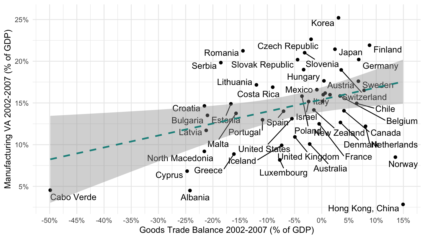
Industry: Change 1991-2018
Code
SNA_TABLE1 %>%
  year_to_date %>%
  filter(MEASURE == "C",
         TRANSACT %in% c("B1_GE", "B1GVB_E", "B11", "P61", "P71")) %>%
  filter(date %in% (paste0(c(1995, 2018), "-01-01") %>% as.Date)) %>%
  select(date, LOCATION, TRANSACT, obsValue) %>%
  spread(TRANSACT, obsValue) %>%
  mutate(IND = B1GVB_E / B1_GE,
         NX = (P61-P71) / B1_GE) %>%
  group_by(LOCATION) %>%
  summarise(NX_mean = NX[2] - NX[1],
            IND_mean = IND[2] - IND[1]) %>%
  na.omit %>%
  left_join(SNA_TABLE1_var$LOCATION, by = "LOCATION") %>%
  ggplot(.) + theme_minimal() + geom_point(aes(x = NX_mean, y = IND_mean)) +
  xlab(expression(Delta~"Goods Trade Balance 1995-2018 (% of GDP)")) +
  ylab(expression(Delta~"Industry VA 1995-2018 (% of GDP)")) +
  scale_x_continuous(breaks = 0.01*seq(-100, 100, 5),
                     labels = percent_format(accuracy = 1)) +
  geom_text_repel(aes(x = NX_mean, y = IND_mean, label = Location), vjust = 0) +
  scale_y_continuous(breaks = 0.01*seq(-100, 100, 5),
                     labels = percent_format(accuracy = 1)) +
  stat_smooth(aes(x = NX_mean, y = IND_mean), linetype = 2,
              method = "lm", color = viridis(3)[2])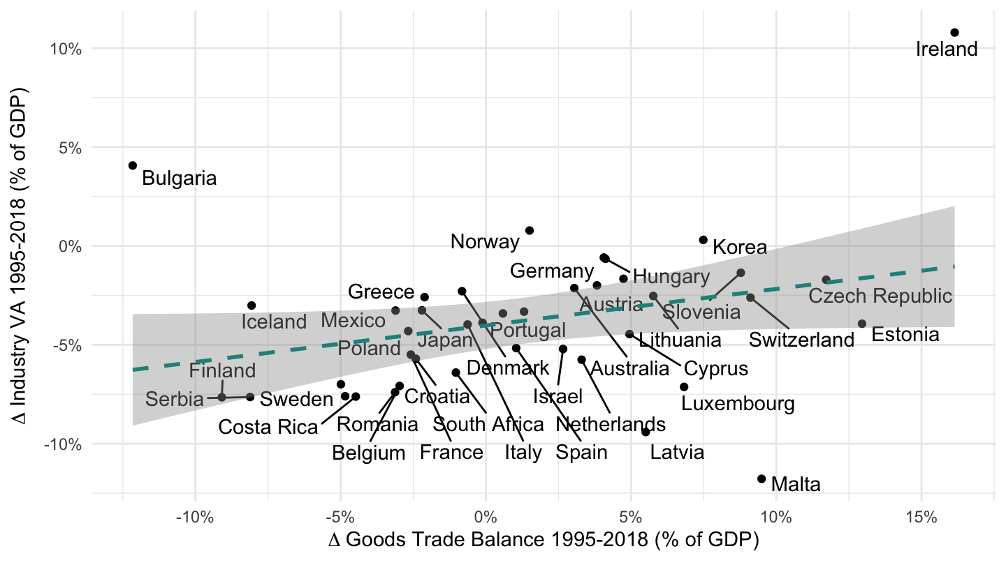
B1_GE - Gross domestic product
“P” Decomposition
Code
SNA_TABLE1 %>%
  filter(LOCATION %in% c("FRA", "DEU", "USA", "GBR"),
         obsTime == "2018",
         MEASURE == "C",
         grepl("^P", TRANSACT) | TRANSACT == "B1_GE") %>%
  select(LOCATION, TRANSACT, obsValue) %>%
  left_join(SNA_TABLE1_var$TRANSACT, by = "TRANSACT") %>%
  spread(LOCATION, obsValue) %>%
  mutate_at(vars(-1, -2), funs(ifelse(is.na(.), "", paste0(round(100*./.[TRANSACT == "B1_GE"], 1), " %")))) %>%
  {if (is_html_output()) datatable(., filter = 'top', rownames = F) else .}
“B” Decomposition
Code
SNA_TABLE1 %>%
  filter(LOCATION %in% c("FRA", "DEU", "USA", "GBR"),
         obsTime == "2018",
         MEASURE == "C",
         grepl("^B", TRANSACT) | TRANSACT == "B1_GE") %>%
  select(LOCATION, TRANSACT, obsValue) %>%
  left_join(SNA_TABLE1_var$TRANSACT, by = "TRANSACT") %>%
  spread(LOCATION, obsValue) %>%
  mutate_at(vars(-1, -2), funs(ifelse(is.na(.), "", paste0(round(100*./.[TRANSACT == "B1_GE"], 1), " %")))) %>%
  {if (is_html_output()) datatable(., filter = 'top', rownames = F) else .}
“D” Decomposition
Code
SNA_TABLE1 %>%
  filter(LOCATION %in% c("FRA", "DEU", "USA", "GBR"),
         obsTime == "2018",
         MEASURE == "C",
         grepl("^D", TRANSACT) | TRANSACT == "B1_GE") %>%
  select(LOCATION, TRANSACT, obsValue) %>%
  left_join(SNA_TABLE1_var$TRANSACT, by = "TRANSACT") %>%
  spread(LOCATION, obsValue) %>%
  mutate_at(vars(-1, -2), funs(ifelse(is.na(.), "", paste0(round(100*./.[TRANSACT == "B1_GE"], 1), " %")))) %>%
  {if (is_html_output()) datatable(., filter = 'top', rownames = F) else .}
All Decomposition
Code
SNA_TABLE1 %>%
  filter(LOCATION %in% c("FRA", "DEU", "USA", "GBR"),
         obsTime == "2018",
         MEASURE == "C") %>%
  select(LOCATION, TRANSACT, obsValue) %>%
  left_join(SNA_TABLE1_var$TRANSACT, by = "TRANSACT") %>%
  spread(LOCATION, obsValue) %>%
  mutate_at(vars(-1, -2), funs(ifelse(is.na(.), "", paste0(round(100*./.[TRANSACT == "B1_GE"], 1), " %")))) %>%
  {if (is_html_output()) datatable(., filter = 'top', rownames = F) else .}
How much data
Code
SNA_TABLE1 %>%
  filter(TRANSACT == "B1_GE",
         MEASURE == "C") %>%
  left_join(SNA_TABLE1_var$LOCATION, by = "LOCATION") %>%
  group_by(LOCATION, UNIT, Location) %>%
  summarise(year_first = first(obsTime),
            year_last = last(obsTime),
            value_last = last(round(obsValue))) %>%
  mutate(Flag = gsub(" ", "-", str_to_lower(gsub(" ", "-", Location))),
         Flag = paste0('<img src="../../icon/flag/vsmall/', Flag, '.png" alt="Flag">')) %>%
  select(Flag, everything()) %>%
  {if (is_html_output()) datatable(., filter = 'top', rownames = F, escape = F) else .}
Compare US and France
Code
SNA_TABLE1 %>%
  filter(LOCATION %in% c("FRA", "USA"),
         obsTime == "2018",
         MEASURE == "C",
         grepl("^P", TRANSACT) | TRANSACT == "B1_GE",
         !grepl("^P51N", TRANSACT)) %>%
  select(LOCATION, TRANSACT, obsValue) %>%
  left_join(SNA_TABLE1_var$TRANSACT, by = "TRANSACT") %>%
  spread(LOCATION, obsValue) %>%
  mutate_at(vars(-1, -2), funs(paste0(round(100*./.[TRANSACT == "B1_GE"], 1), " %"))) %>%
{if (is_html_output()) print_table(.) else .}| TRANSACT | Transact | FRA | USA |
|---|---|---|---|
| B1_GE | Gross domestic product (expenditure approach) | 100 % | 100 % |
| P3 | Final consumption expenditure | 77.2 % | 81.9 % |
| P3_P5 | Domestic demand | 101 % | 103 % |
| P31S13 | Individual consumption expenditure of general government | 15.2 % | 6 % |
| P31S14 | Final consumption expenditure of households | 51.8 % | 65.8 % |
| P31S14_S15 | Households and Non-profit institutions serving households | 53.9 % | 67.9 % |
| P31S15 | Final consumption expenditure of non-profit institutions serving households | 2.1 % | 2.1 % |
| P32S13 | Collective consumption expenditure of general government | 8.1 % | 8 % |
| P3S13 | Final consumption expenditure of general government | 23.3 % | 14 % |
| P41 | of which: Actual individual consumption | 69.1 % | 73.9 % |
| P5 | Gross capital formation | 23.9 % | 21 % |
| P51 | Gross fixed capital formation | 22.9 % | 20.8 % |
| P52 | Changes in inventories | 0.9 % | 0.3 % |
| P52_P53 | Changes in inventories and acquisitions less disposals of valuables | 1 % | 0.3 % |
| P53 | Acquisitions less disposals of valuables | 0 % | NA % |
| P6 | Exports of goods and services | 31.7 % | 12.3 % |
| P61 | Exports of goods | 22.1 % | 8.1 % |
| P62 | Exports of services | 9.6 % | 4.2 % |
| P7 | Imports of goods and services | 32.8 % | 15.2 % |
| P71 | Imports of goods | 23.7 % | 12.4 % |
| P72 | Imports of services | 9.1 % | 2.8 % |
France
Net Exports - Total, Goods, Services
Code
SNA_TABLE1 %>%
  filter(LOCATION == "FRA",
         MEASURE == "C",
         TRANSACT %in% c("B1_GE", "P61", "P71", "P62", "P72", "P6", "P7")) %>%
  left_join(SNA_TABLE1_var$TRANSACT, by = "TRANSACT") %>%
  left_join(SNA_TABLE1_var$LOCATION, by = "LOCATION") %>%
  year_to_date %>%
  group_by(date) %>%
  mutate(obsValue = obsValue / obsValue[TRANSACT == "B1_GE"]) %>%
  filter(TRANSACT != "B1_GE") %>%
  select(date, TRANSACT, obsValue) %>%
  na.omit %>%
  spread(TRANSACT, obsValue) %>%
  transmute(date,
            `Tous` = P6 - P7,
            `Biens` = P61 - P71,
            `Services` = P62 - P72) %>%
  gather(variable, value, -date) %>%
  ggplot() + geom_line(aes(x = date, y = value, color = variable)) +
  scale_color_manual(values = c("brown", "orange", "black")) + theme_minimal() +
  scale_x_date(breaks = seq(1920, 2100, 5) %>% paste0("-01-01") %>% as.Date,
               labels = date_format("%Y")) +
  theme(legend.position = c(0.85, 0.9),
        legend.title = element_blank()) +
  scale_y_continuous(breaks = 0.01*seq(-60, 60, 1),
                     labels = scales::percent_format(accuracy = 1)) +
  ylab("Exportations Nettes (% du PIB)") + xlab("") +
  geom_hline(yintercept = 0, linetype = "dotted")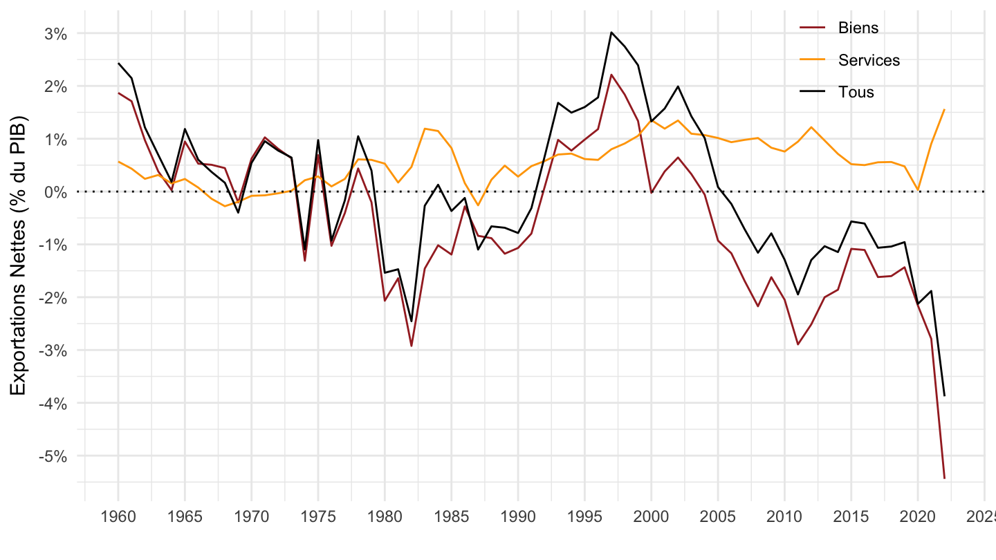
Exports, Imports - Goods, Services
Code
SNA_TABLE1 %>%
  filter(LOCATION == "FRA",
         MEASURE == "C",
         TRANSACT %in% c("B1_GE", "P61", "P71", "P62", "P72")) %>%
  left_join(SNA_TABLE1_var$TRANSACT, by = "TRANSACT") %>%
  year_to_date %>%
  group_by(date) %>%
  mutate(obsValue = obsValue / obsValue[TRANSACT == "B1_GE"]) %>%
  filter(TRANSACT != "B1_GE") %>%
  ggplot() + geom_line() + theme_minimal() +
  aes(x = date, y = obsValue, color = Transact, linetype = Transact) +
  scale_color_manual(values = c(viridis(3)[1], viridis(3)[2], viridis(3)[1], viridis(3)[2])) +
  scale_linetype_manual(values = c("solid", "solid", "dashed", "dashed")) +
  ylab("% of GDP") + xlab("") +
  scale_x_date(breaks = seq(1920, 2100, 5) %>% paste0("-01-01") %>% as.Date,
               labels = date_format("%Y")) +
  theme(legend.position = c(0.15, 0.9),
        legend.title = element_blank()) +
  scale_y_continuous(breaks = 0.01*seq(-60, 60, 1),
                     labels = scales::percent_format(accuracy = 1))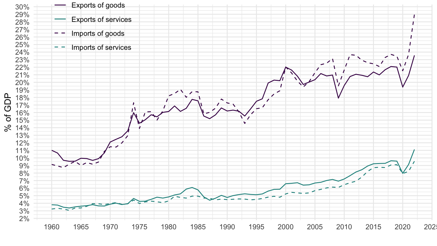
Manufacturing (Bn€)
France, Germany, Italy
Code
SNA_TABLE1 %>%
  filter(LOCATION %in% c("FRA", "ITA", "DEU"),
         MEASURE == "V",
         TRANSACT %in% c("B1GVC")) %>%
  year_to_date %>%
  filter(date >= as.Date("1980-01-01")) %>%
  left_join(SNA_TABLE1_var$LOCATION, by = "LOCATION") %>%
  select(date, Location, TRANSACT, obsValue) %>%
  spread(TRANSACT, obsValue) %>%
  mutate(obsValue = B1GVC/1000) %>%
  left_join(colors, by = c("Location" = "country")) %>%
  ggplot() + geom_line(aes(x = date, y = obsValue, color = color)) +
  scale_color_identity() + theme_minimal() + add_3flags +
  scale_x_date(breaks = seq(1920, 2100, 5) %>% paste0("-01-01") %>% as.Date,
               labels = date_format("%Y")) +
  scale_y_continuous(breaks = seq(0, 4000, 100),
                     labels = scales::dollar_format(accuracy = 1, su = "Bn€", p = "")) +
  ylab("Manufacturing Value Added (Bn)") + xlab("")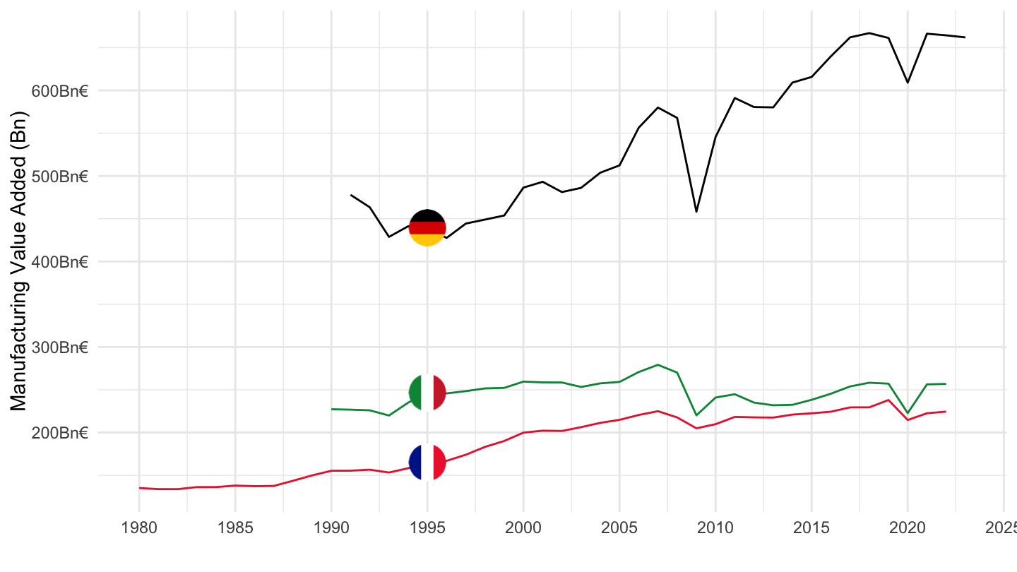
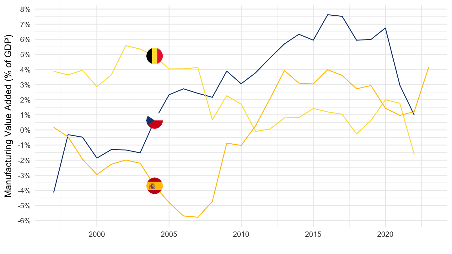
Manufacturing, Industry, Industry without Manufacturing (% of GDP)
Australia
Code
SNA_TABLE1 %>%
  filter(LOCATION %in% c("AUS"),
         MEASURE == "C",
         TRANSACT %in% c("B1_GE", "B1GVC", "B1GVB_E")) %>%
  year_to_date %>%
  select(date, TRANSACT, obsValue) %>%
  spread(TRANSACT, obsValue) %>%
  transmute(date,
            `Manufacturing` = B1GVC / B1_GE,
            `Industry` = B1GVB_E / B1_GE,
            `Industry excl. Manufacturing` = (B1GVB_E - B1GVC) / B1_GE) %>%
  gather(Transact, value, -date) %>%
  na.omit %>%
  ggplot() + geom_line() + theme_minimal() +
  aes(x = date, y = value, color = Transact, linetype = Transact) +
  scale_color_manual(values = viridis(4)[1:3]) +  ylab("% of GDP") + xlab("") +
  scale_x_date(breaks = seq(1920, 2100, 5) %>% paste0("-01-01") %>% as.Date,
               labels = date_format("%Y")) +
  theme(legend.position = c(0.2, 0.7),
        legend.title = element_blank()) +
  scale_y_continuous(breaks = 0.01*seq(-60, 60, 1),
                     labels = scales::percent_format(accuracy = 1))
France
Code
SNA_TABLE1 %>%
  filter(LOCATION %in% c("FRA"),
         MEASURE == "C",
         TRANSACT %in% c("B1_GE", "B1GVC", "B1GVB_E")) %>%
  year_to_date %>%
  select(date, TRANSACT, obsValue) %>%
  spread(TRANSACT, obsValue) %>%
  transmute(date,
            `Manufacturing` = B1GVC / B1_GE,
            `Industry` = B1GVB_E / B1_GE,
            `Industry excl. Manufacturing` = (B1GVB_E - B1GVC) / B1_GE) %>%
  gather(Transact, value, -date) %>%
  na.omit %>%
  ggplot() + geom_line() + theme_minimal() +
  aes(x = date, y = value, color = Transact, linetype = Transact) +
  scale_color_manual(values = viridis(4)[1:3]) +  ylab("% of GDP") + xlab("") +
  scale_x_date(breaks = seq(1920, 2100, 5) %>% paste0("-01-01") %>% as.Date,
               labels = date_format("%Y")) +
  theme(legend.position = c(0.2, 0.7),
        legend.title = element_blank()) +
  scale_y_continuous(breaks = 0.01*seq(-60, 60, 1),
                     labels = scales::percent_format(accuracy = 1))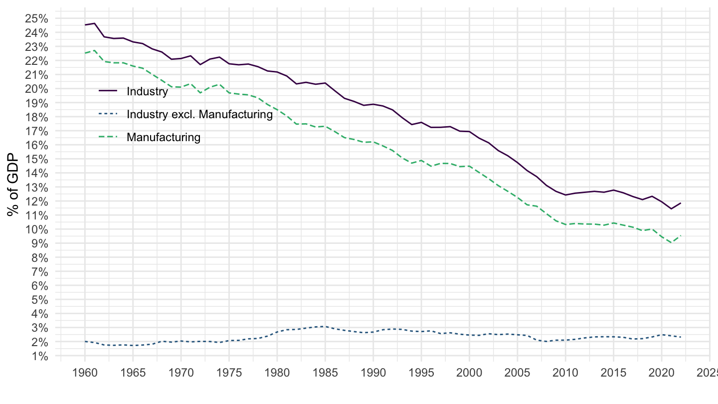
Germany
Code
SNA_TABLE1 %>%
  filter(LOCATION %in% c("DEU"),
         MEASURE == "C",
         TRANSACT %in% c("B1_GE", "B1GVC", "B1GVB_E")) %>%
  year_to_date %>%
  select(date, TRANSACT, obsValue) %>%
  spread(TRANSACT, obsValue) %>%
  transmute(date,
            `Manufacturing` = B1GVC / B1_GE,
            `Industry` = B1GVB_E / B1_GE,
            `Industry excl. Manufacturing` = (B1GVB_E - B1GVC) / B1_GE) %>%
  gather(Transact, value, -date) %>%
  na.omit %>%
  ggplot() + geom_line() + theme_minimal() +
  aes(x = date, y = value, color = Transact, linetype = Transact) +
  scale_color_manual(values = viridis(4)[1:3]) +  ylab("% of GDP") + xlab("") +
  scale_x_date(breaks = seq(1920, 2100, 5) %>% paste0("-01-01") %>% as.Date,
               labels = date_format("%Y")) +
  theme(legend.position = c(0.2, 0.7),
        legend.title = element_blank()) +
  scale_y_continuous(breaks = 0.01*seq(-60, 60, 1),
                     labels = scales::percent_format(accuracy = 1))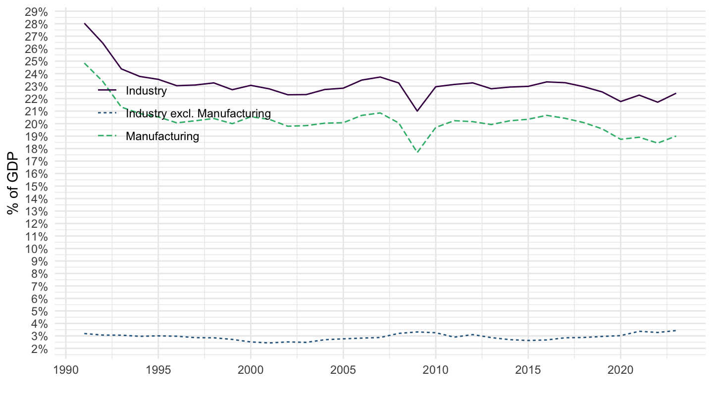
Netherlands
Code
SNA_TABLE1 %>%
  filter(LOCATION %in% c("NLD"),
         MEASURE == "C",
         TRANSACT %in% c("B1_GE", "B1GVC", "B1GVB_E")) %>%
  year_to_date %>%
  select(date, TRANSACT, obsValue) %>%
  spread(TRANSACT, obsValue) %>%
  transmute(date,
            `Manufacturing` = B1GVC / B1_GE,
            `Industry` = B1GVB_E / B1_GE,
            `Industry excl. Manufacturing` = (B1GVB_E - B1GVC) / B1_GE) %>%
  gather(Transact, value, -date) %>%
  na.omit %>%
  ggplot() + geom_line() + theme_minimal() +
  aes(x = date, y = value, color = Transact, linetype = Transact) +
  scale_color_manual(values = viridis(4)[1:3]) +  ylab("% of GDP") + xlab("") +
  scale_x_date(breaks = seq(1920, 2100, 5) %>% paste0("-01-01") %>% as.Date,
               labels = date_format("%Y")) +
  theme(legend.position = c(0.2, 0.7),
        legend.title = element_blank()) +
  scale_y_continuous(breaks = 0.01*seq(-60, 60, 1),
                     labels = scales::percent_format(accuracy = 1))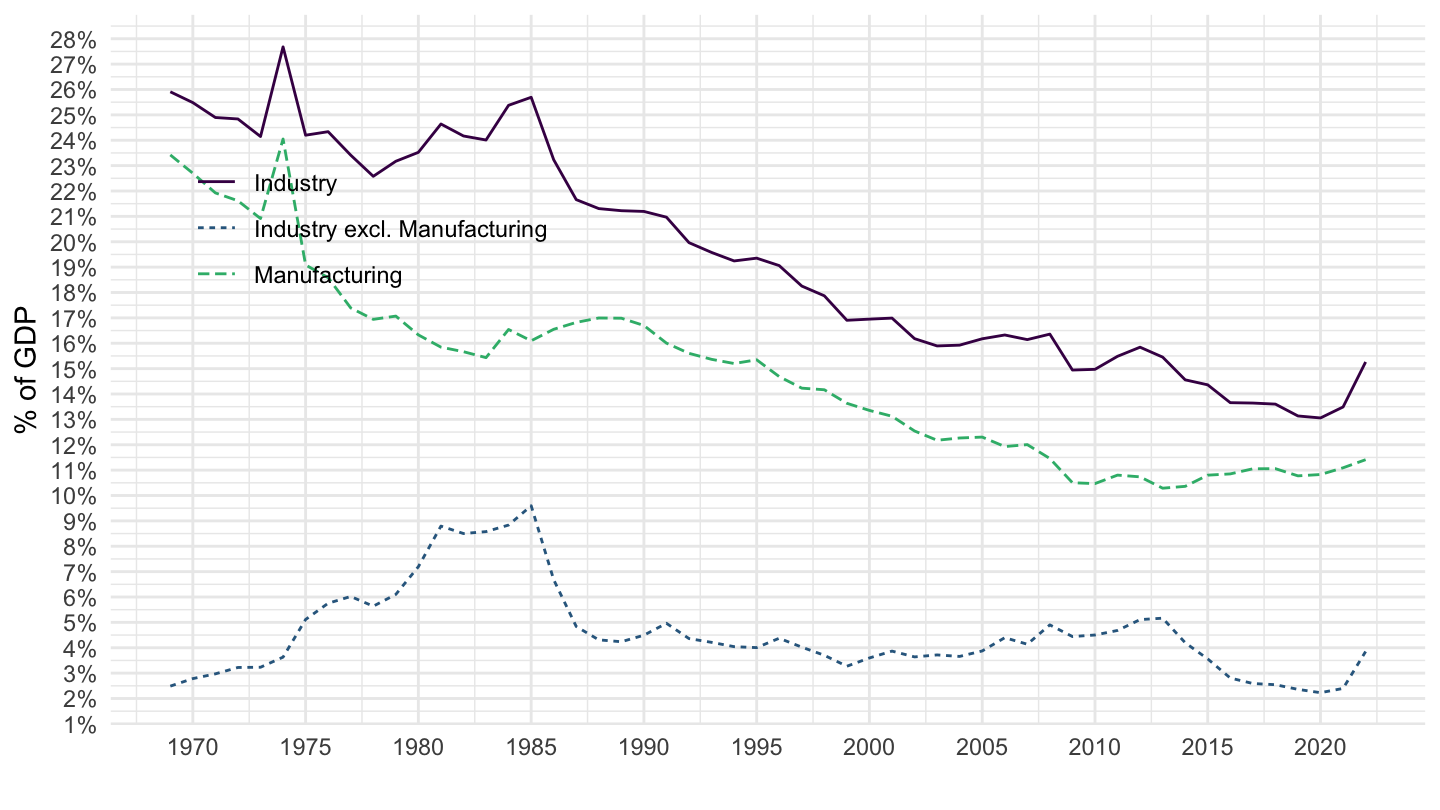
NOR
Code
SNA_TABLE1 %>%
  filter(LOCATION %in% c("NOR"),
         MEASURE == "C",
         TRANSACT %in% c("B1_GE", "B1GVC", "B1GVB_E")) %>%
  year_to_date %>%
  select(date, TRANSACT, obsValue) %>%
  spread(TRANSACT, obsValue) %>%
  transmute(date,
            `Manufacturing` = B1GVC / B1_GE,
            `Industry` = B1GVB_E / B1_GE,
            `Industry excl. Manufacturing` = (B1GVB_E - B1GVC) / B1_GE) %>%
  gather(Transact, value, -date) %>%
  na.omit %>%
  ggplot() + geom_line() + theme_minimal() +
  aes(x = date, y = value, color = Transact, linetype = Transact) +
  scale_color_manual(values = viridis(4)[1:3]) +  ylab("% of GDP") + xlab("") +
  scale_x_date(breaks = seq(1920, 2100, 5) %>% paste0("-01-01") %>% as.Date,
               labels = date_format("%Y")) +
  theme(legend.position = c(0.2, 0.7),
        legend.title = element_blank()) +
  scale_y_continuous(breaks = 0.01*seq(-60, 60, 1),
                     labels = scales::percent_format(accuracy = 1))
Manufacturing, Industry (% of GDP)
Australia
Code
SNA_TABLE1 %>%
  filter(LOCATION %in% c("AUS"),
         MEASURE == "C",
         TRANSACT %in% c("B1_GE", "B1GVC", "B1GVB_E")) %>%
  year_to_date %>%
  select(date, TRANSACT, obsValue) %>%
  spread(TRANSACT, obsValue) %>%
  transmute(date,
            `Manufacturing` = B1GVC / B1_GE,
            `Industry` = B1GVB_E / B1_GE) %>%
  gather(Transact, value, -date) %>%
  na.omit %>%
  ggplot() + geom_line() + theme_minimal() +
  aes(x = date, y = value, color = Transact, linetype = Transact) +
  scale_color_manual(values = viridis(3)[1:2]) +  ylab("% of GDP") + xlab("") +
  scale_x_date(breaks = seq(1920, 2100, 5) %>% paste0("-01-01") %>% as.Date,
               labels = date_format("%Y")) +
  theme(legend.position = c(0.2, 0.2),
        legend.title = element_blank()) +
  scale_y_continuous(breaks = 0.01*seq(-60, 60, 1),
                     labels = scales::percent_format(accuracy = 1))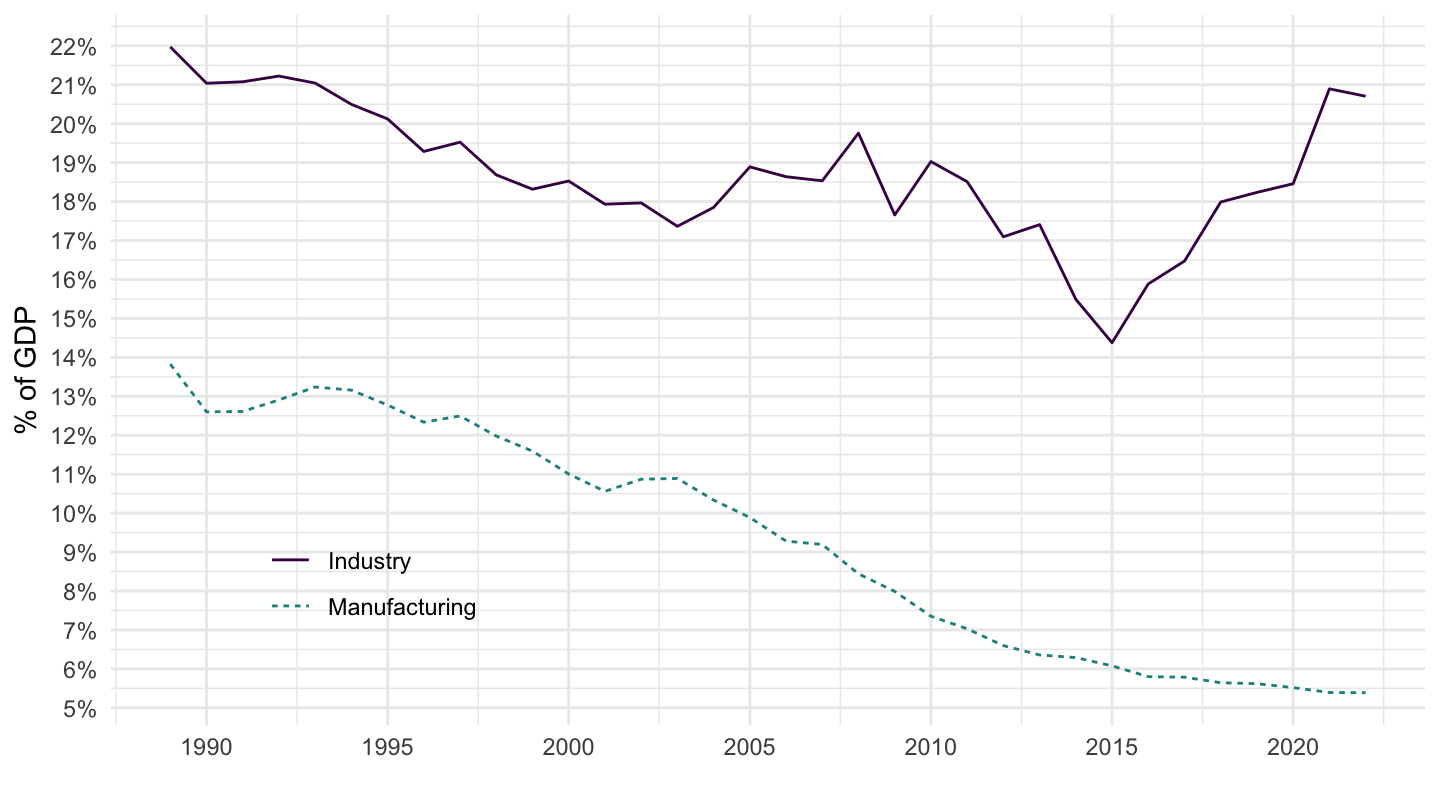
France
Code
SNA_TABLE1 %>%
  filter(LOCATION %in% c("FRA"),
         MEASURE == "C",
         TRANSACT %in% c("B1_GE", "B1GVC", "B1GVB_E")) %>%
  year_to_date %>%
  select(date, TRANSACT, obsValue) %>%
  spread(TRANSACT, obsValue) %>%
  transmute(date,
            `Manufacturing` = B1GVC / B1_GE,
            `Industry` = B1GVB_E / B1_GE) %>%
  gather(Transact, value, -date) %>%
  na.omit %>%
  ggplot() + geom_line() + theme_minimal() +
  aes(x = date, y = value, color = Transact, linetype = Transact) +
  scale_color_manual(values = viridis(3)[1:2]) +  ylab("% of GDP") + xlab("") +
  scale_x_date(breaks = seq(1920, 2100, 5) %>% paste0("-01-01") %>% as.Date,
               labels = date_format("%Y")) +
  theme(legend.position = c(0.8, 0.8),
        legend.title = element_blank()) +
  scale_y_continuous(breaks = 0.01*seq(-60, 60, 1),
                     labels = scales::percent_format(accuracy = 1))
Germany
Code
SNA_TABLE1 %>%
  filter(LOCATION %in% c("DEU"),
         MEASURE == "C",
         TRANSACT %in% c("B1_GE", "B1GVC", "B1GVB_E")) %>%
  year_to_date %>%
  select(date, TRANSACT, obsValue) %>%
  spread(TRANSACT, obsValue) %>%
  transmute(date,
            `Manufacturing` = B1GVC / B1_GE,
            `Industry` = B1GVB_E / B1_GE) %>%
  gather(Transact, value, -date) %>%
  na.omit %>%
  ggplot() + geom_line() + theme_minimal() +
  aes(x = date, y = value, color = Transact, linetype = Transact) +
  scale_color_manual(values = viridis(3)[1:2]) +  ylab("% of GDP") + xlab("") +
  scale_x_date(breaks = seq(1920, 2100, 5) %>% paste0("-01-01") %>% as.Date,
               labels = date_format("%Y")) +
  theme(legend.position = c(0.8, 0.8),
        legend.title = element_blank()) +
  scale_y_continuous(breaks = 0.01*seq(-60, 60, 1),
                     labels = scales::percent_format(accuracy = 1))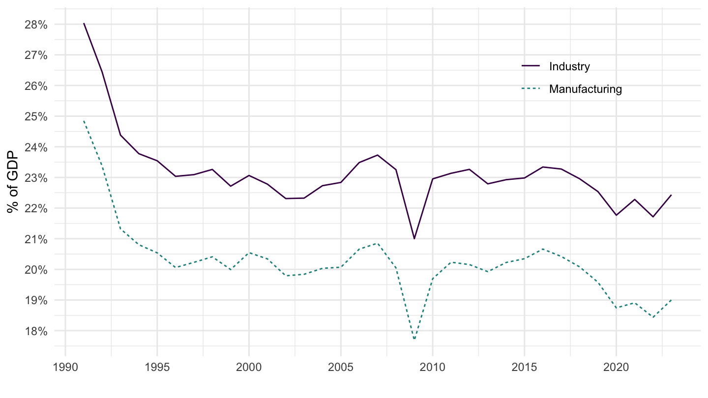
Greece
Code
SNA_TABLE1 %>%
  filter(LOCATION %in% c("GRC"),
         MEASURE == "C",
         TRANSACT %in% c("B1_GE", "B1GVC", "B1GVB_E")) %>%
  year_to_date %>%
  select(date, TRANSACT, obsValue) %>%
  spread(TRANSACT, obsValue) %>%
  transmute(date,
            `Manufacturing` = B1GVC / B1_GE,
            `Industry` = B1GVB_E / B1_GE) %>%
  gather(Transact, value, -date) %>%
  na.omit %>%
  ggplot() + geom_line() + theme_minimal() +
  aes(x = date, y = value, color = Transact, linetype = Transact) +
  scale_color_manual(values = viridis(3)[1:2]) +  ylab("% of GDP") + xlab("") +
  scale_x_date(breaks = seq(1920, 2100, 5) %>% paste0("-01-01") %>% as.Date,
               labels = date_format("%Y")) +
  theme(legend.position = c(0.8, 0.8),
        legend.title = element_blank()) +
  scale_y_continuous(breaks = 0.01*seq(-60, 60, 1),
                     labels = scales::percent_format(accuracy = 1))
Industry (% of GDP)
Number of observations
Code
SNA_TABLE1 %>%
  filter(MEASURE == "C",
         TRANSACT %in% c("B1GVB_E", "B1_GE")) %>%
  year_to_date %>%
  left_join(SNA_TABLE1_var$LOCATION, by = "LOCATION") %>%
  group_by(LOCATION, Location) %>%
  select(date, Location, LOCATION, TRANSACT, obsValue) %>%
  spread(TRANSACT, obsValue) %>%
  mutate(obsValue = B1GVB_E / B1_GE) %>%
  summarise(first = first(date),
            last = last(date),
            last_value = last(obsValue),
            Nobs = n()) %>%
  arrange(last_value) %>%
  mutate(Flag = gsub(" ", "-", str_to_lower(gsub(" ", "-", Location))),
         Flag = paste0('<img src="../../icon/flag/vsmall/', Flag, '.png" alt="Flag">')) %>%
  select(Flag, everything()) %>%
  {if (is_html_output()) datatable(., filter = 'top', rownames = F, escape = F) else .}
Spain, France, Germany, Italy, Greece
1980-
Code
SNA_TABLE1 %>%
  filter(LOCATION %in% c("FRA", "ITA", "DEU", "ESP", "GRC", "EA19"),
         MEASURE == "C",
         TRANSACT %in% c("B1_GE", "B1GVB_E")) %>%
  year_to_date %>%
  filter(date >= as.Date("1980-01-01")) %>%
  left_join(SNA_TABLE1_var$LOCATION, by = "LOCATION") %>%
  select(date, Location, LOCATION, TRANSACT, obsValue) %>%
  spread(TRANSACT, obsValue) %>%
  mutate(obsValue = B1GVB_E / B1_GE) %>%
  mutate(Location = ifelse(LOCATION == "EA19", "Europe", Location)) %>%
  left_join(colors, by = c("Location" = "country")) %>%
  ggplot() + geom_line(aes(x = date, y = obsValue, color = color)) +
  ylab("Industry Value Added (% of GDP)") + xlab("") +
  scale_color_identity() + theme_minimal() + add_6flags +
  scale_x_date(breaks = seq(1920, 2100, 5) %>% paste0("-01-01") %>% as.Date,
               labels = date_format("%Y")) +
  scale_y_continuous(breaks = 0.01*seq(-60, 60, 1),
                     labels = scales::percent_format(accuracy = 1))
1995-
Code
SNA_TABLE1 %>%
  filter(LOCATION %in% c("FRA", "ITA", "DEU", "ESP", "GRC", "EA19", "USA"),
         MEASURE == "C",
         TRANSACT %in% c("B1_GE", "B1GVB_E")) %>%
  year_to_date %>%
  filter(date >= as.Date("1995-01-01")) %>%
  left_join(SNA_TABLE1_var$LOCATION, by = "LOCATION") %>%
  select(date, Location, LOCATION, TRANSACT, obsValue) %>%
  spread(TRANSACT, obsValue) %>%
  mutate(obsValue = B1GVB_E / B1_GE) %>%
  mutate(Location = ifelse(LOCATION == "EA19", "Europe", Location)) %>%
  left_join(colors, by = c("Location" = "country")) %>%
  mutate(color = ifelse(LOCATION == "USA", color2, color)) %>%
  ggplot() + geom_line(aes(x = date, y = obsValue, color = color)) +
  ylab("Valeur ajoutée dans l'industrie (% du PIB)") + xlab("") +
  scale_color_identity() + theme_minimal() + add_7flags +
  scale_x_date(breaks = seq(1995, 2100, 2) %>% paste0("-01-01") %>% as.Date,
               labels = date_format("%Y")) +
  scale_y_continuous(breaks = 0.01*seq(-60, 60, 1),
                     labels = scales::percent_format(accuracy = 1))
1995-
Code
SNA_TABLE1 %>%
  filter(LOCATION %in% c("FRA", "ITA", "DEU", "ESP", "GRC", "EA19", "USA", "GBR"),
         MEASURE == "C",
         TRANSACT %in% c("B1_GE", "B1GVB_E")) %>%
  year_to_date %>%
  filter(date >= as.Date("1995-01-01")) %>%
  left_join(SNA_TABLE1_var$LOCATION, by = "LOCATION") %>%
  select(date, Location, LOCATION, TRANSACT, obsValue) %>%
  spread(TRANSACT, obsValue) %>%
  mutate(obsValue = B1GVB_E / B1_GE) %>%
  mutate(Location = ifelse(LOCATION == "EA19", "Europe", Location)) %>%
  left_join(colors, by = c("Location" = "country")) %>%
  mutate(color = ifelse(LOCATION == "USA", color2, color)) %>%
  ggplot() + geom_line(aes(x = date, y = obsValue, color = color)) +
  ylab("Valeur ajoutée dans l'industrie (% du PIB)") + xlab("") +
  scale_color_identity() + theme_minimal() + add_8flags +
  scale_x_date(breaks = seq(1995, 2100, 2) %>% paste0("-01-01") %>% as.Date,
               labels = date_format("%Y")) +
  scale_y_continuous(breaks = 0.01*seq(-60, 60, 1),
                     labels = scales::percent_format(accuracy = 1))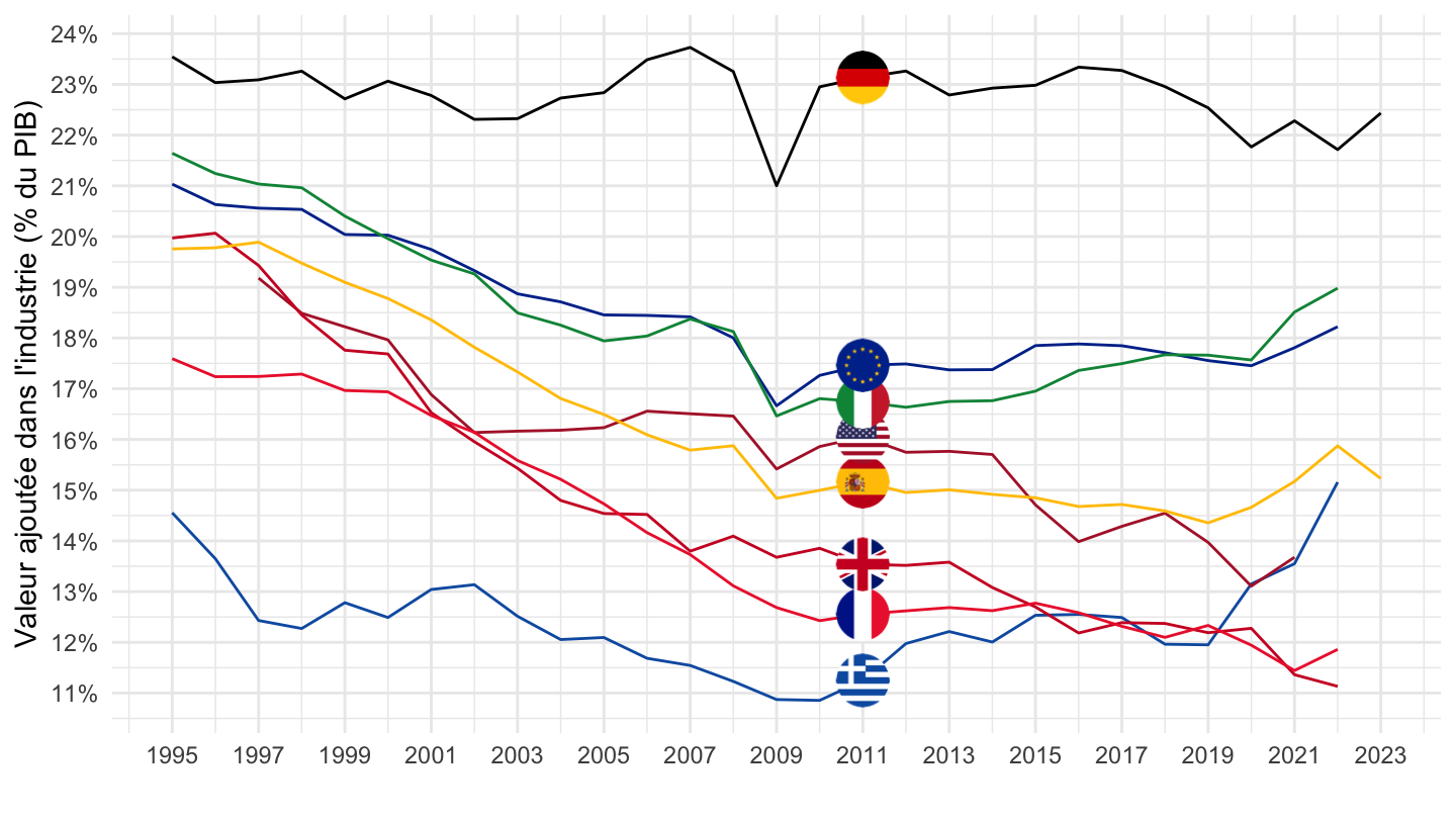
1995-
% of GDP
Code
SNA_TABLE1 %>%
  filter(LOCATION %in% c("FRA", "USA", "GBR", "EA19"),
         MEASURE == "C",
         TRANSACT %in% c("B1_GE", "B1GVB_E")) %>%
  year_to_date %>%
  filter(date >= as.Date("1995-01-01")) %>%
  left_join(SNA_TABLE1_var$LOCATION, by = "LOCATION") %>%
  select(date, Location, LOCATION, TRANSACT, obsValue) %>%
  spread(TRANSACT, obsValue) %>%
  mutate(obsValue = B1GVB_E / B1_GE) %>%
  mutate(Location = ifelse(LOCATION == "EA19", "Europe", Location)) %>%
  left_join(colors, by = c("Location" = "country")) %>%
  mutate(color = ifelse(LOCATION == "FRA", color2, color),
         color = ifelse(LOCATION == "EA19", color2, color)) %>%
  ggplot() + geom_line(aes(x = date, y = obsValue, color = color)) +
  ylab("Valeur ajoutée dans l'industrie (% du PIB)") + xlab("") +
  scale_color_identity() + theme_minimal() + add_4flags +
  scale_x_date(breaks = seq(1995, 2100, 2) %>% paste0("-01-01") %>% as.Date,
               labels = date_format("%Y")) +
  scale_y_continuous(breaks = 0.01*seq(-60, 60, 1),
                     labels = scales::percent_format(accuracy = 1))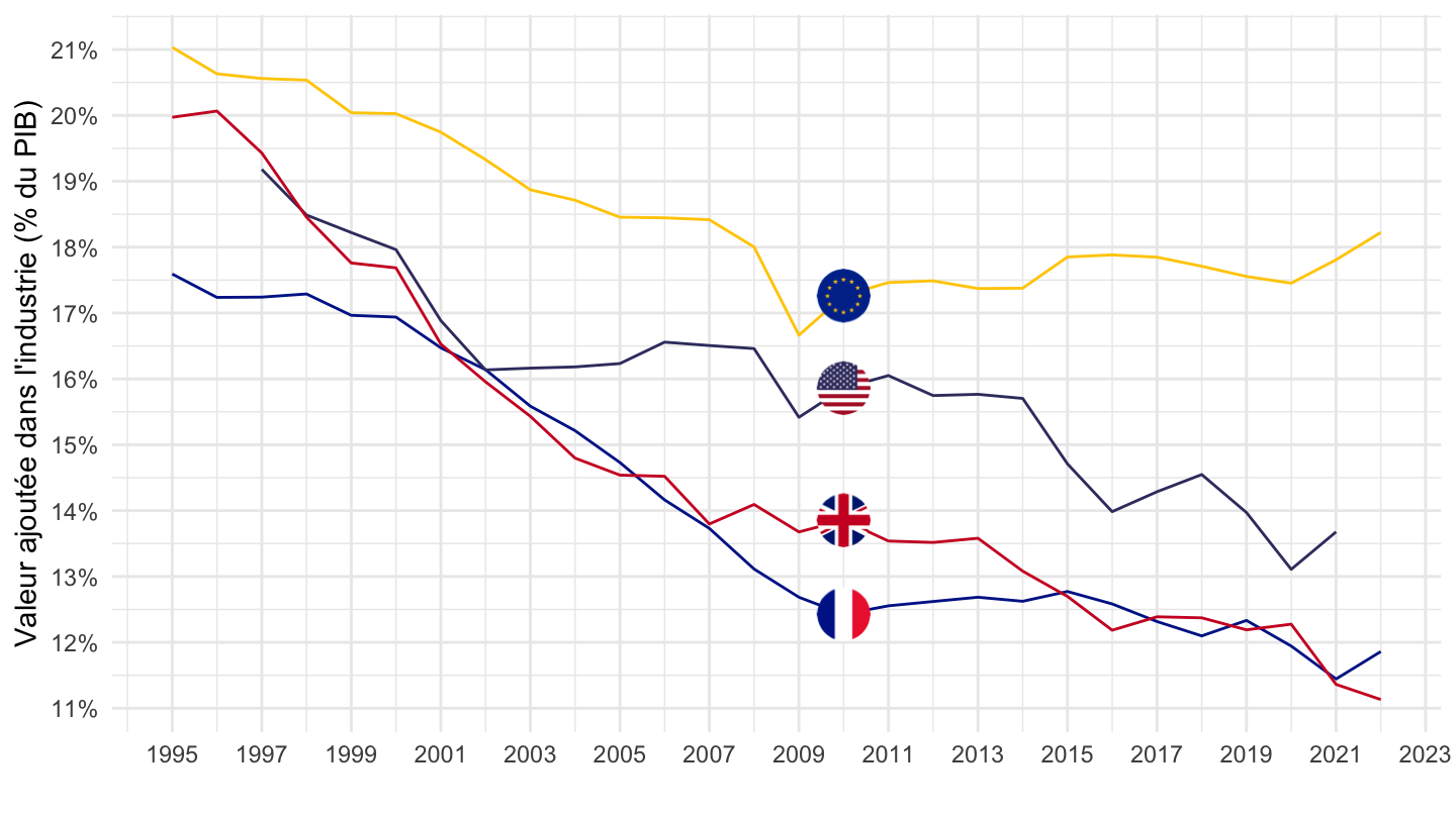
Valeur Ajoutée
Code
SNA_TABLE1 %>%
  filter(LOCATION %in% c("FRA", "USA", "GBR", "EA19"),
         MEASURE == "C",
         TRANSACT %in% c("B1GVB_E")) %>%
  year_to_date %>%
  filter(date >= as.Date("1997-01-01")) %>%
  left_join(SNA_TABLE1_var$LOCATION, by = "LOCATION") %>%
  select(date, Location, LOCATION, TRANSACT, obsValue) %>%
  group_by(Location) %>%
  arrange(date) %>%
  mutate(obsValue = 100*obsValue/obsValue[date == as.Date("1997-01-01")]) %>%
  mutate(Location = ifelse(LOCATION == "EA19", "Europe", Location)) %>%
  left_join(colors, by = c("Location" = "country")) %>%
  mutate(color = ifelse(LOCATION == "FRA", color2, color),
         color = ifelse(LOCATION == "EA19", color2, color)) %>%
  ggplot() + geom_line(aes(x = date, y = obsValue, color = color)) +
  ylab("Valeur ajoutée dans l'industrie (Indice)") + xlab("") +
  scale_color_identity() + theme_minimal() + add_4flags +
  scale_x_date(breaks = seq(1995, 2100, 2) %>% paste0("-01-01") %>% as.Date,
               labels = date_format("%Y")) +
  scale_y_continuous(breaks = seq(100, 400, 10))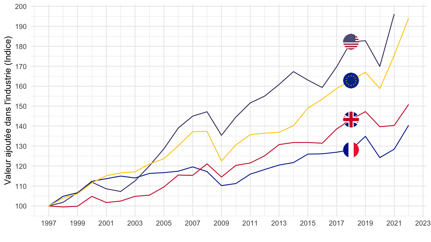
1995-
Code
SNA_TABLE1 %>%
  filter(LOCATION %in% c("FRA", "DEU", "EA19", "USA", "GBR"),
         MEASURE == "C",
         TRANSACT %in% c("B1_GE", "B1GVB_E")) %>%
  year_to_date %>%
  filter(date >= as.Date("1995-01-01")) %>%
  left_join(SNA_TABLE1_var$LOCATION, by = "LOCATION") %>%
  select(date, Location, LOCATION, TRANSACT, obsValue) %>%
  spread(TRANSACT, obsValue) %>%
  mutate(obsValue = B1GVB_E / B1_GE) %>%
  mutate(Location = ifelse(LOCATION == "EA19", "Europe", Location)) %>%
  left_join(colors, by = c("Location" = "country")) %>%
  mutate(color = ifelse(LOCATION == "USA", color2, color),
         color = ifelse(LOCATION == "FRA", color2, color)) %>%
  ggplot() + geom_line(aes(x = date, y = obsValue, color = color)) +
  ylab("Valeur ajoutée dans l'industrie (% du PIB)") + xlab("") +
  scale_color_identity() + theme_minimal() + add_5flags +
  scale_x_date(breaks = seq(1995, 2100, 2) %>% paste0("-01-01") %>% as.Date,
               labels = date_format("%Y")) +
  scale_y_continuous(breaks = 0.01*seq(-60, 60, 1),
                     labels = scales::percent_format(accuracy = 1))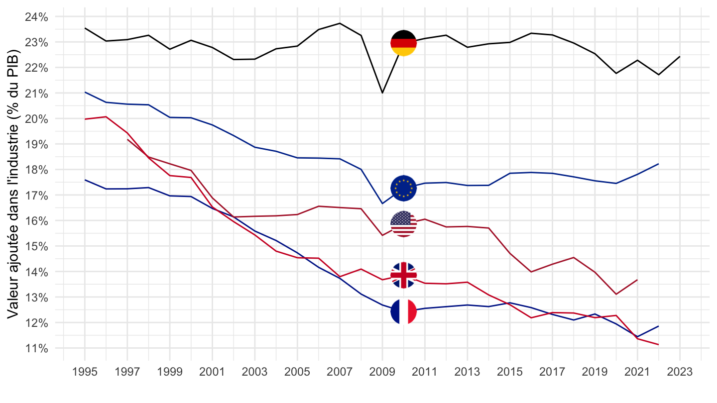
1995-
Code
SNA_TABLE1 %>%
  filter(LOCATION %in% c("FRA", "ITA", "DEU", "ESP", "GRC", "EA19", "USA"),
         MEASURE == "C",
         TRANSACT %in% c("B1_GE", "B1GVC")) %>%
  year_to_date %>%
  filter(date >= as.Date("1995-01-01")) %>%
  left_join(SNA_TABLE1_var$LOCATION, by = "LOCATION") %>%
  select(date, Location, LOCATION, TRANSACT, obsValue) %>%
  spread(TRANSACT, obsValue) %>%
  mutate(obsValue = B1GVC / B1_GE) %>%
  mutate(Location = ifelse(LOCATION == "EA19", "Europe", Location)) %>%
  left_join(colors, by = c("Location" = "country")) %>%
  mutate(color = ifelse(LOCATION == "USA", color2, color)) %>%
  ggplot() + geom_line(aes(x = date, y = obsValue, color = color)) +
  ylab("Valeur ajoutée dans l'industrie manufacturière (% du PIB)") + xlab("") +
  scale_color_identity() + theme_minimal() + add_7flags +
  scale_x_date(breaks = seq(1995, 2100, 2) %>% paste0("-01-01") %>% as.Date,
               labels = date_format("%Y")) +
  scale_y_continuous(breaks = 0.01*seq(-60, 60, 1),
                     labels = scales::percent_format(accuracy = 1))
Spain, France, Germany, Italy, Greece
Code
SNA_TABLE1 %>%
  filter(LOCATION %in% c("FRA", "GRC", "EA19"),
         MEASURE == "C",
         TRANSACT %in% c("B1_GE", "B1GVB_E")) %>%
  year_to_date %>%
  left_join(SNA_TABLE1_var$LOCATION, by = "LOCATION") %>%
  select(date, Location, LOCATION, TRANSACT, obsValue) %>%
  spread(TRANSACT, obsValue) %>%
  mutate(obsValue = B1GVB_E / B1_GE) %>%
  mutate(Location = ifelse(LOCATION == "EA19", "Europe", Location)) %>%
  left_join(colors, by = c("Location" = "country")) %>%
  ggplot() + geom_line(aes(x = date, y = obsValue, color = color)) +
  ylab("Industry Value Added (% of GDP)") + xlab("") +
  scale_color_identity() + theme_minimal() + add_3flags +
  geom_rect(data = data_frame(start = as.Date("1945-01-01"),
                                end = as.Date("1975-01-01")),
              aes(xmin = start, xmax = end, ymin = -Inf, ymax = +Inf),
              fill = viridis(4)[4], alpha = 0.2) +
  scale_x_date(breaks = seq(1920, 2100, 5) %>% paste0("-01-01") %>% as.Date,
               labels = date_format("%Y")) +
  scale_y_continuous(breaks = 0.01*seq(-60, 60, 1),
                     labels = scales::percent_format(accuracy = 1))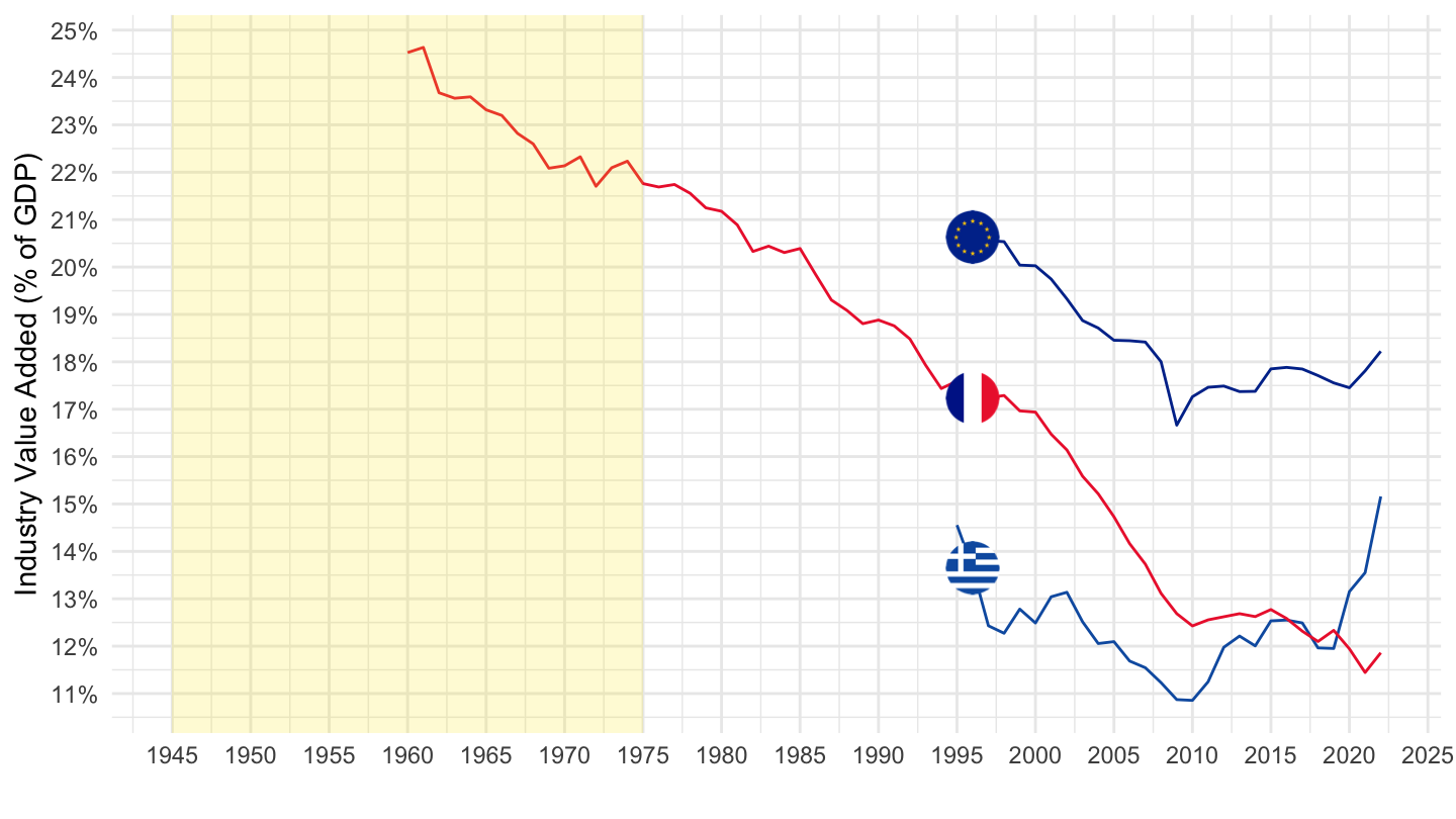
Manufacturing (% of GDP)
Number of observations
Code
SNA_TABLE1 %>%
  filter(MEASURE == "C",
         TRANSACT %in% c("B1GVC")) %>%
  year_to_date %>%
  left_join(SNA_TABLE1_var$LOCATION, by = "LOCATION") %>%
  group_by(LOCATION, Location) %>%
  summarise(first = first(date),
            last = last(date),
            Nobs = n()) %>%
  arrange(first) %>%
  mutate(Flag = gsub(" ", "-", str_to_lower(gsub(" ", "-", Location))),
         Flag = paste0('<img src="../../icon/flag/vsmall/', Flag, '.png" alt="Flag">')) %>%
  select(Flag, everything()) %>%
  {if (is_html_output()) datatable(., filter = 'top', rownames = F, escape = F) else .}
B1GVC - Manufacturing Value Added
United States, United Kingdom, France
All-
Code
SNA_TABLE1 %>%
  filter(LOCATION %in% c("FRA", "USA", "GBR"),
         MEASURE == "C",
         TRANSACT %in% c("B1_GE", "B1GVC")) %>%
  year_to_date %>%
  left_join(SNA_TABLE1_var$LOCATION, by = "LOCATION") %>%
  select(date, Location, TRANSACT, obsValue) %>%
  spread(TRANSACT, obsValue) %>%
  mutate(obsValue = B1GVC / B1_GE) %>%
  left_join(colors, by = c("Location" = "country")) %>%
  ggplot() + geom_line(aes(x = date, y = obsValue, color = color)) +
  ylab("Manufacturing Value Added (% of GDP)") + xlab("") +
  scale_color_identity() + theme_minimal() + add_3flags +
  scale_x_date(breaks = seq(1920, 2100, 5) %>% paste0("-01-01") %>% as.Date,
               labels = date_format("%Y")) +
  scale_y_continuous(breaks = 0.01*seq(-60, 60, 1),
                     labels = scales::percent_format(accuracy = 1))
1995-
Code
SNA_TABLE1 %>%
  filter(LOCATION %in% c("FRA", "USA", "GBR"),
         MEASURE == "C",
         TRANSACT %in% c("B1_GE", "B1GVC")) %>%
  year_to_date %>%
  filter(date >= as.Date("1995-01-01")) %>%
  left_join(SNA_TABLE1_var$LOCATION, by = "LOCATION") %>%
  select(date, Location, TRANSACT, obsValue) %>%
  spread(TRANSACT, obsValue) %>%
  mutate(obsValue = B1GVC / B1_GE) %>%
  left_join(colors, by = c("Location" = "country")) %>%
  ggplot() + geom_line(aes(x = date, y = obsValue, color = color)) +
  ylab("Manufacturing Value Added (% of GDP)") + xlab("") +
  scale_color_identity() + theme_minimal() + add_3flags +
  scale_x_date(breaks = seq(1920, 2100, 5) %>% paste0("-01-01") %>% as.Date,
               labels = date_format("%Y")) +
  scale_y_continuous(breaks = 0.01*seq(-60, 60, 1),
                     labels = scales::percent_format(accuracy = 1))
Korea, Singapore
Code
SNA_TABLE1 %>%
  filter(LOCATION %in% c("KOR", "SGP", "DNK"),
         MEASURE == "C",
         TRANSACT %in% c("B1_GE", "B1GVC")) %>%
  year_to_date %>%
  #filter(date >= as.Date("1995-01-01")) %>%
  left_join(SNA_TABLE1_var$LOCATION, by = "LOCATION") %>%
  select(date, Location, TRANSACT, obsValue) %>%
  spread(TRANSACT, obsValue) %>%
  mutate(obsValue = B1GVC / B1_GE) %>%
  left_join(colors, by = c("Location" = "country")) %>%
  ggplot() + geom_line(aes(x = date, y = obsValue, color = color)) +
  ylab("Manufacturing Value Added (% of GDP)") + xlab("") +
  scale_color_identity() + theme_minimal() + add_3flags +
  scale_x_date(breaks = seq(1920, 2100, 5) %>% paste0("-01-01") %>% as.Date,
               labels = date_format("%Y")) +
  scale_y_continuous(breaks = 0.01*seq(-60, 60, 1),
                     labels = scales::percent_format(accuracy = 1))
Australia, Eurozone, Japan
%
Code
SNA_TABLE1 %>%
  filter(LOCATION %in% c("AUS", "JPN", "EA19"),
         MEASURE == "C",
         TRANSACT %in% c("B1_GE", "B1GVC")) %>%
  year_to_date %>%
  filter(date >= as.Date("1980-01-01")) %>%
  left_join(SNA_TABLE1_var$LOCATION, by = "LOCATION") %>%
  select(date, Location, LOCATION, TRANSACT, obsValue) %>%
  spread(TRANSACT, obsValue) %>%
  mutate(obsValue = B1GVC / B1_GE) %>%
  mutate(Location = ifelse(LOCATION == "EA19", "Europe", Location)) %>%
  left_join(colors, by = c("Location" = "country")) %>%
  ggplot() + geom_line(aes(x = date, y = obsValue, color = color)) +
  ylab("Manufacturing Value Added (% of GDP)") + xlab("") +
  scale_color_identity() + theme_minimal() + add_3flags +
  scale_x_date(breaks = seq(1920, 2100, 5) %>% paste0("-01-01") %>% as.Date,
               labels = date_format("%Y")) +
  scale_y_continuous(breaks = 0.01*seq(-60, 60, 1),
                     labels = scales::percent_format(accuracy = 1))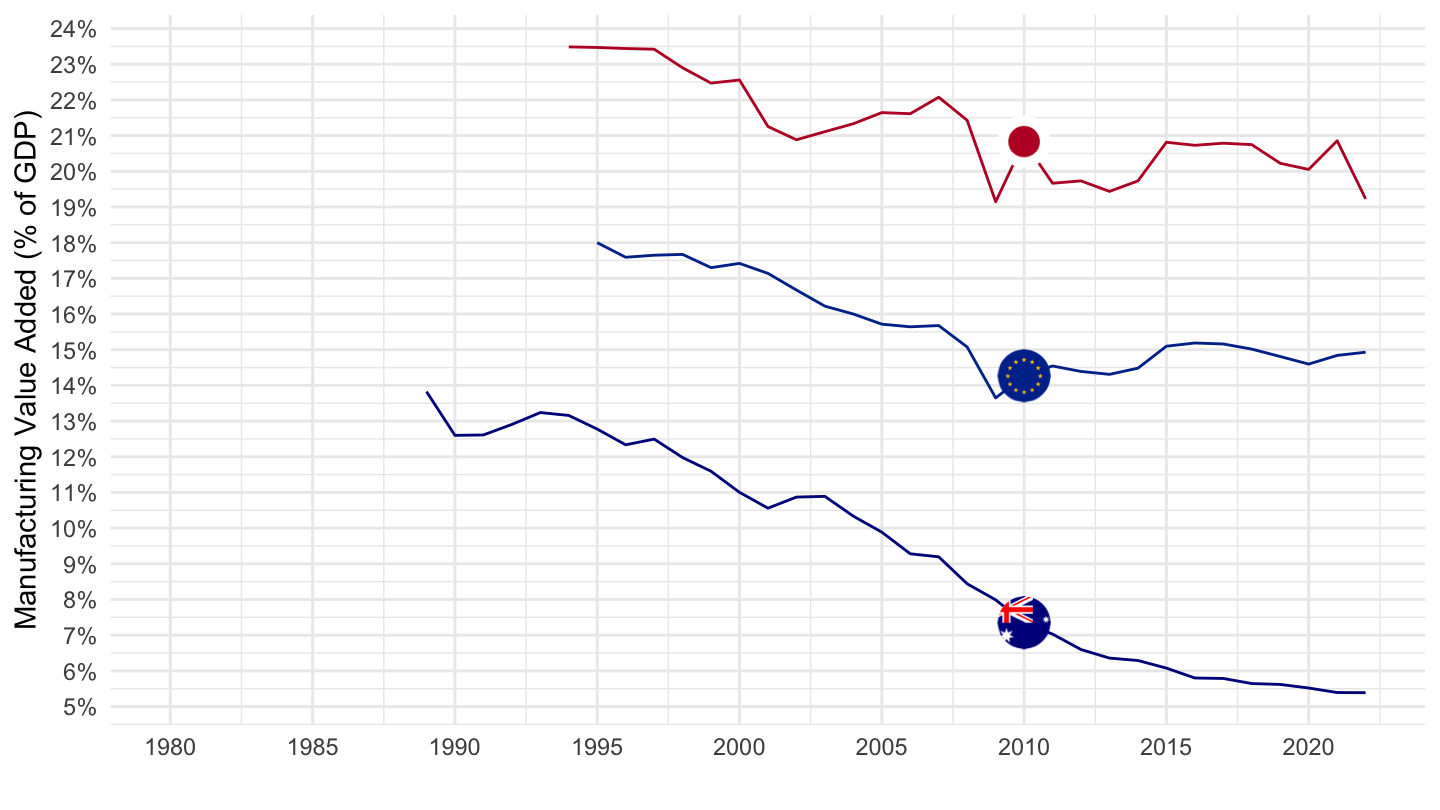
Log
Code
SNA_TABLE1 %>%
  filter(LOCATION %in% c("AUS", "JPN", "EA19"),
         MEASURE == "C",
         TRANSACT %in% c("B1_GE", "B1GVC")) %>%
  year_to_date %>%
  filter(date >= as.Date("1980-01-01")) %>%
  left_join(SNA_TABLE1_var$LOCATION, by = "LOCATION") %>%
  select(date, Location, LOCATION, TRANSACT, obsValue) %>%
  spread(TRANSACT, obsValue) %>%
  mutate(obsValue = B1GVC / B1_GE) %>%
  mutate(Location = ifelse(LOCATION == "EA19", "Europe", Location)) %>%
  left_join(colors, by = c("Location" = "country")) %>%
  ggplot() + geom_line(aes(x = date, y = obsValue, color = color)) +
  ylab("Manufacturing Value Added (% of GDP)") + xlab("") +
  scale_color_identity() + theme_minimal() + add_3flags +
  scale_x_date(breaks = seq(1920, 2100, 5) %>% paste0("-01-01") %>% as.Date,
               labels = date_format("%Y")) +
  scale_y_log10(breaks = 0.01*seq(-60, 60, 1),
                     labels = scales::percent_format(accuracy = 1))
France, Germany, Italy
Viridis
Code
SNA_TABLE1 %>%
  filter(LOCATION %in% c("FRA", "ITA", "DEU"),
         MEASURE == "C",
         TRANSACT %in% c("B1_GE", "B1GVC")) %>%
  year_to_date %>%
  filter(date >= as.Date("1980-01-01")) %>%
  left_join(SNA_TABLE1_var$LOCATION, by = "LOCATION") %>%
  select(date, Location, TRANSACT, obsValue) %>%
  spread(TRANSACT, obsValue) %>%
  mutate(B1GVC_B1_GE = B1GVC / B1_GE) %>%
  ggplot() + geom_line() +
  aes(x = date, y = B1GVC_B1_GE, color = Location) +
  scale_color_manual(values = viridis(4)[1:3]) +
  theme_minimal() +
  scale_x_date(breaks = seq(1920, 2100, 5) %>% paste0("-01-01") %>% as.Date,
               labels = date_format("%Y")) +
  theme(legend.position = c(0.15, 0.2),
        legend.title = element_blank()) +
  scale_y_continuous(breaks = 0.01*seq(-60, 60, 1),
                     labels = scales::percent_format(accuracy = 1)) +
  ylab("Manufacturing Value Added (% of GDP)") + xlab("")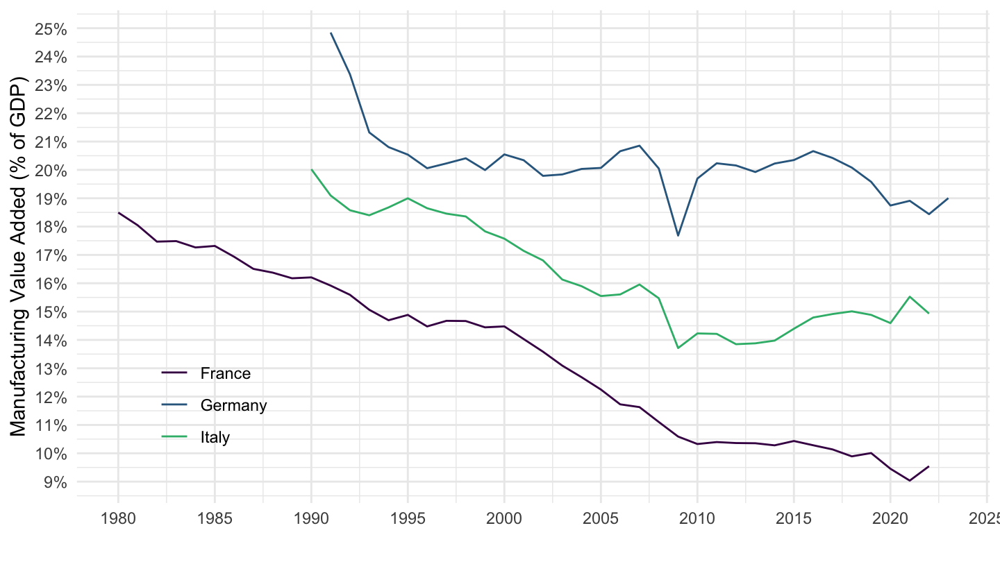
Flags
All
Code
SNA_TABLE1 %>%
  filter(LOCATION %in% c("FRA", "ITA", "DEU", "USA"),
         MEASURE == "C",
         TRANSACT %in% c("B1_GE", "B1GVC")) %>%
  year_to_date %>%
  #filter(date >= as.Date("1980-01-01")) %>%
  left_join(SNA_TABLE1_var$LOCATION, by = "LOCATION") %>%
  select(date, Location, TRANSACT, obsValue) %>%
  spread(TRANSACT, obsValue) %>%
  mutate(obsValue = B1GVC / B1_GE) %>%
  left_join(colors, by = c("Location" = "country")) %>%
  ggplot() + geom_line(aes(x = date, y = obsValue, color = color)) +
  ylab("Manufacturing Value Added (% of GDP)") + xlab("") +
  scale_color_identity() + theme_minimal() + add_4flags +
  scale_x_date(breaks = seq(1920, 2100, 5) %>% paste0("-01-01") %>% as.Date,
               labels = date_format("%Y")) +
  scale_y_continuous(breaks = 0.01*seq(-60, 60, 1),
                     labels = scales::percent_format(accuracy = 1))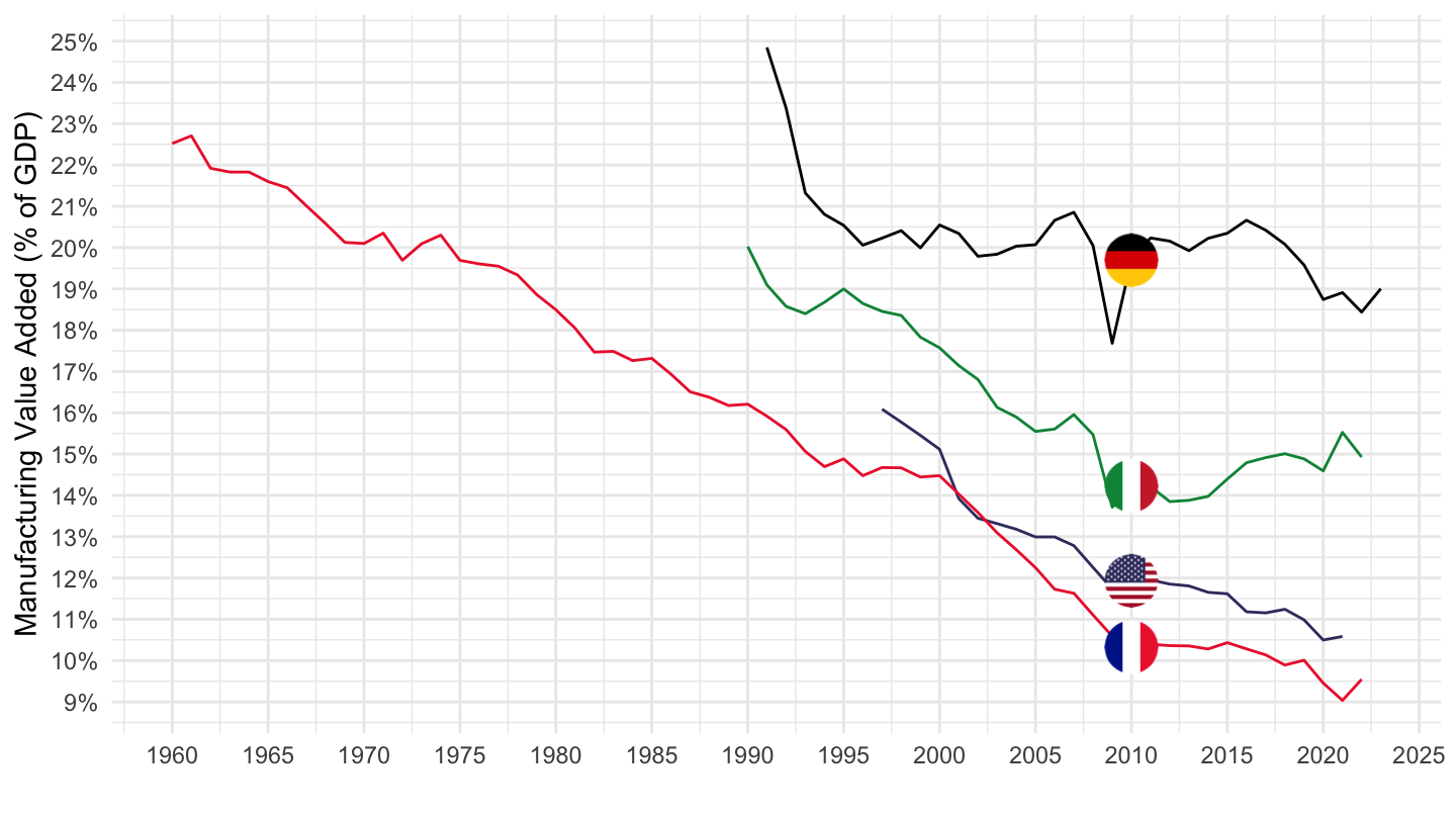
1990-
Code
SNA_TABLE1 %>%
  filter(LOCATION %in% c("FRA", "ITA", "DEU", "USA"),
         MEASURE == "C",
         TRANSACT %in% c("B1_GE", "B1GVC")) %>%
  year_to_date %>%
  filter(date >= as.Date("1990-01-01")) %>%
  left_join(SNA_TABLE1_var$LOCATION, by = "LOCATION") %>%
  select(date, Location, TRANSACT, obsValue) %>%
  spread(TRANSACT, obsValue) %>%
  mutate(obsValue = B1GVC / B1_GE) %>%
  left_join(colors, by = c("Location" = "country")) %>%
  filter(date >= as.Date("1990-01-01")) %>%
  ggplot() + geom_line(aes(x = date, y = obsValue, color = color)) +
  ylab("Manufacturing Value Added (% of GDP)") + xlab("") +
  scale_color_identity() + theme_minimal() + add_4flags +
  scale_x_date(breaks = seq(1920, 2100, 5) %>% paste0("-01-01") %>% as.Date,
               labels = date_format("%Y")) +
  scale_y_continuous(breaks = 0.01*seq(-60, 60, 1),
                     labels = scales::percent_format(accuracy = 1))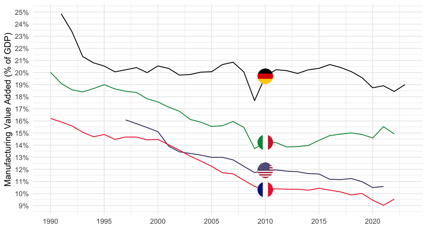
1995-
Code
SNA_TABLE1 %>%
  filter(LOCATION %in% c("FRA", "ITA", "DEU", "USA"),
         MEASURE == "C",
         TRANSACT %in% c("B1_GE", "B1GVC")) %>%
  year_to_date %>%
  filter(date >= as.Date("1980-01-01")) %>%
  left_join(SNA_TABLE1_var$LOCATION, by = "LOCATION") %>%
  select(date, Location, TRANSACT, obsValue) %>%
  spread(TRANSACT, obsValue) %>%
  mutate(obsValue = B1GVC / B1_GE) %>%
  left_join(colors, by = c("Location" = "country")) %>%
  filter(date >= as.Date("1995-01-01")) %>%
  ggplot() + geom_line(aes(x = date, y = obsValue, color = color)) +
  ylab("Manufacturing Value Added (% of GDP)") + xlab("") +
  scale_color_identity() + theme_minimal() + add_4flags +
  scale_x_date(breaks = seq(1920, 2100, 5) %>% paste0("-01-01") %>% as.Date,
               labels = date_format("%Y")) +
  scale_y_continuous(breaks = 0.01*seq(-60, 60, 1),
                     labels = scales::percent_format(accuracy = 1))
Spain, France, Germany, Italy
Code
SNA_TABLE1 %>%
  filter(LOCATION %in% c("FRA", "ITA", "DEU", "ESP"),
         MEASURE == "C",
         TRANSACT %in% c("B1_GE", "B1GVC")) %>%
  year_to_date %>%
  filter(date >= as.Date("1980-01-01")) %>%
  left_join(SNA_TABLE1_var$LOCATION, by = "LOCATION") %>%
  select(date, Location, TRANSACT, obsValue) %>%
  spread(TRANSACT, obsValue) %>%
  mutate(obsValue = B1GVC / B1_GE) %>%
  left_join(colors, by = c("Location" = "country")) %>%
  ggplot() + geom_line(aes(x = date, y = obsValue, color = color)) +
  ylab("Manufacturing Value Added (% of GDP)") + xlab("") +
  scale_color_identity() + theme_minimal() + add_4flags +
  scale_x_date(breaks = seq(1920, 2100, 5) %>% paste0("-01-01") %>% as.Date,
               labels = date_format("%Y")) +
  scale_y_continuous(breaks = 0.01*seq(-60, 60, 1),
                     labels = scales::percent_format(accuracy = 1))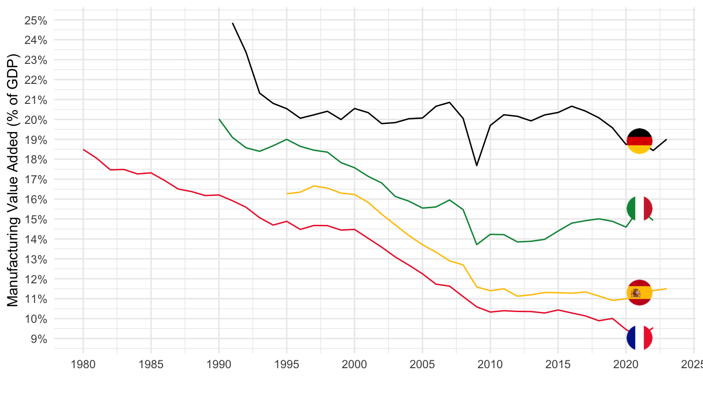
Greece, Portugal, Spain
Code
SNA_TABLE1 %>%
  filter(LOCATION %in% c("GRC", "PRT", "ESP"),
         MEASURE == "C",
         TRANSACT %in% c("B1_GE", "B1GVC")) %>%
  year_to_date %>%
  filter(date >= as.Date("1995-01-01")) %>%
  left_join(SNA_TABLE1_var$LOCATION, by = "LOCATION") %>%
  select(date, Location, TRANSACT, obsValue) %>%
  spread(TRANSACT, obsValue) %>%
  mutate(obsValue = B1GVC / B1_GE) %>%
  left_join(colors, by = c("Location" = "country")) %>%
  ggplot() + geom_line(aes(x = date, y = obsValue, color = color)) +
  ylab("Manufacturing Value Added (% of GDP)") + xlab("") +
  scale_color_identity() + theme_minimal() + add_3flags +
  scale_x_date(breaks = seq(1920, 2100, 5) %>% paste0("-01-01") %>% as.Date,
               labels = date_format("%Y")) +
  scale_y_continuous(breaks = 0.01*seq(-60, 60, 1),
                     labels = scales::percent_format(accuracy = 1))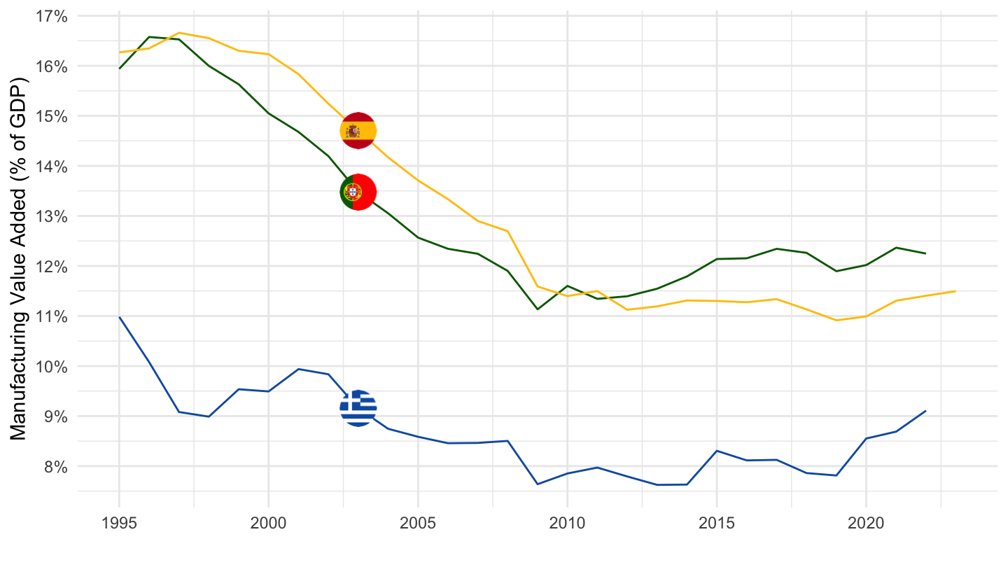
Greece, Portugal, Spain, Italy
Code
SNA_TABLE1 %>%
  filter(LOCATION %in% c("GRC", "PRT", "ESP", "ITA"),
         MEASURE == "C",
         TRANSACT %in% c("B1_GE", "B1GVC")) %>%
  year_to_date %>%
  filter(date >= as.Date("1995-01-01")) %>%
  left_join(SNA_TABLE1_var$LOCATION, by = "LOCATION") %>%
  select(date, Location, TRANSACT, obsValue) %>%
  spread(TRANSACT, obsValue) %>%
  mutate(obsValue = B1GVC / B1_GE) %>%
  left_join(colors, by = c("Location" = "country")) %>%
  ggplot() + geom_line(aes(x = date, y = obsValue, color = color)) +
  ylab("Manufacturing Value Added (% of GDP)") + xlab("") +
  scale_color_identity() + theme_minimal() + add_4flags +
  scale_x_date(breaks = seq(1920, 2100, 5) %>% paste0("-01-01") %>% as.Date,
               labels = date_format("%Y")) +
  scale_y_continuous(breaks = 0.01*seq(-60, 60, 1),
                     labels = scales::percent_format(accuracy = 1))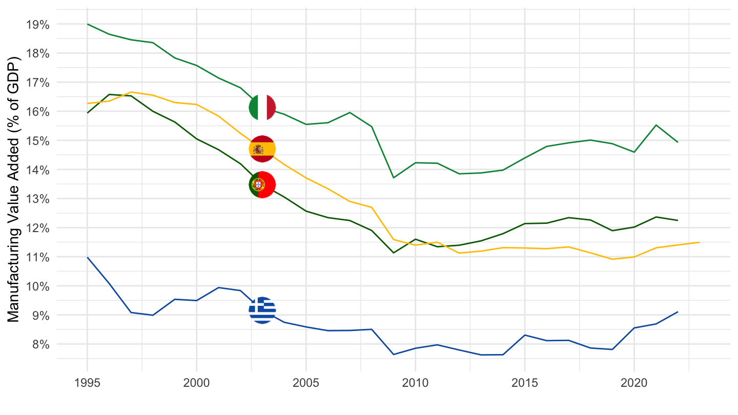
France, Germany, United States
Code
SNA_TABLE1 %>%
  filter(LOCATION %in% c("FRA", "USA", "DEU"),
         MEASURE == "C",
         TRANSACT %in% c("B1_GE", "B1GVC")) %>%
  year_to_date %>%
  filter(date >= as.Date("1980-01-01")) %>%
  left_join(SNA_TABLE1_var$LOCATION, by = "LOCATION") %>%
  select(date, Location, TRANSACT, obsValue) %>%
  spread(TRANSACT, obsValue) %>%
  mutate(obsValue = B1GVC / B1_GE) %>%
  left_join(colors, by = c("Location" = "country")) %>%
  ggplot() + geom_line(aes(x = date, y = obsValue, color = color)) +
  ylab("Manufacturing Value Added (% of GDP)") + xlab("") +
  scale_color_identity() + theme_minimal() + add_3flags +
  scale_x_date(breaks = seq(1920, 2100, 5) %>% paste0("-01-01") %>% as.Date,
               labels = date_format("%Y")) +
  scale_y_continuous(breaks = 0.01*seq(-60, 60, 1),
                     labels = scales::percent_format(accuracy = 1))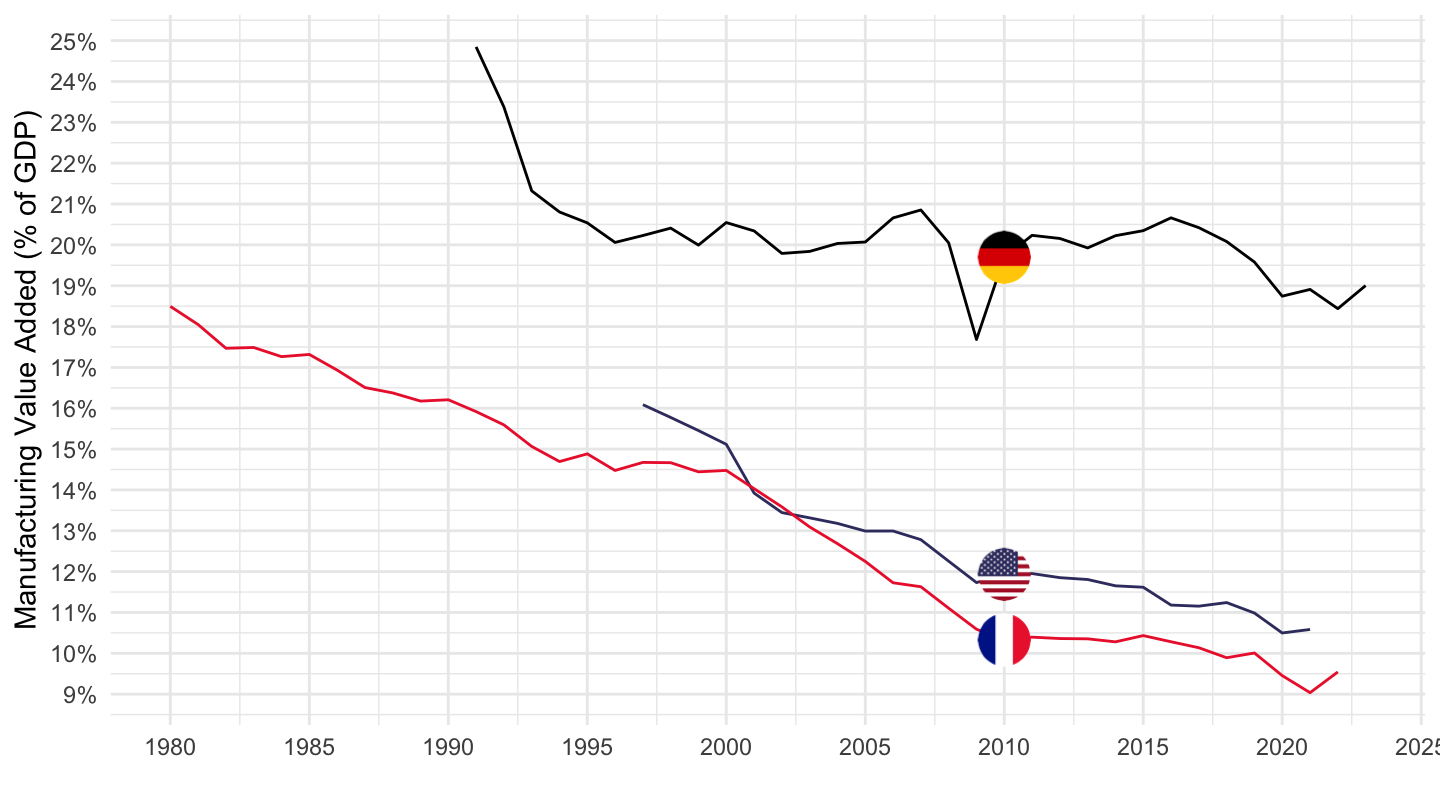
France, Germany, OECD
Code
SNA_TABLE1 %>%
  filter(LOCATION %in% c("FRA", "OECD", "DEU"),
         MEASURE == "C",
         TRANSACT %in% c("B1_GE", "B1GVC")) %>%
  year_to_date %>%
  filter(date >= as.Date("1980-01-01")) %>%
  left_join(SNA_TABLE1_var$LOCATION, by = "LOCATION") %>%
  select(date, Location, LOCATION, TRANSACT, obsValue) %>%
  spread(TRANSACT, obsValue) %>%
  mutate(obsValue = B1GVC / B1_GE) %>%
  mutate(Location = ifelse(LOCATION == "OECD", "OECD members", Location)) %>%
  left_join(colors, by = c("Location" = "country")) %>%
  ggplot() + geom_line(aes(x = date, y = obsValue, color = color)) +
  ylab("Manufacturing Value Added (% of GDP)") + xlab("") +
  scale_color_identity() + theme_minimal() + add_3flags +
  scale_x_date(breaks = seq(1920, 2100, 5) %>% paste0("-01-01") %>% as.Date,
               labels = date_format("%Y")) +
  scale_y_continuous(breaks = 0.01*seq(-60, 60, 1),
                     labels = scales::percent_format(accuracy = 1))
France, Denmark, Germany, Austria
Code
SNA_TABLE1 %>%
  filter(LOCATION %in% c("FRA", "DNK", "DEU", "AUT"),
         MEASURE == "C",
         TRANSACT %in% c("B1_GE", "B1GVC")) %>%
  year_to_date %>%
  filter(date >= as.Date("1980-01-01")) %>%
  left_join(SNA_TABLE1_var$LOCATION, by = "LOCATION") %>%
  select(date, Location, TRANSACT, obsValue) %>%
  spread(TRANSACT, obsValue) %>%
  mutate(obsValue = B1GVC / B1_GE) %>%
  left_join(colors, by = c("Location" = "country")) %>%
  ggplot() + geom_line(aes(x = date, y = obsValue, color = color)) +
  ylab("Manufacturing Value Added (% of GDP)") + xlab("") +
  scale_color_identity() + theme_minimal() + add_4flags +
  scale_x_date(breaks = seq(1920, 2100, 5) %>% paste0("-01-01") %>% as.Date,
               labels = date_format("%Y")) +
  scale_y_continuous(breaks = 0.01*seq(-60, 60, 1),
                     labels = scales::percent_format(accuracy = 1))
France, Germany, Italy
Code
SNA_TABLE1 %>%
  filter(LOCATION %in% c("FRA", "ITA", "DEU"),
         MEASURE == "C",
         TRANSACT %in% c("B1_GE", "B1GVC")) %>%
  year_to_date %>%
  filter(date >= as.Date("1994-01-01")) %>%
  left_join(SNA_TABLE1_var$LOCATION, by = "LOCATION") %>%
  select(date, Location, TRANSACT, obsValue) %>%
  spread(TRANSACT, obsValue) %>%
  mutate(obsValue = B1GVC / B1_GE) %>%
  left_join(colors, by = c("Location" = "country")) %>%
  ggplot() + geom_line(aes(x = date, y = obsValue, color = color)) +
  ylab("Manufacturing Value Added (% of GDP)") + xlab("") +
  scale_color_identity() + theme_minimal() + add_3flags +
  scale_x_date(breaks = seq(1920, 2100, 5) %>% paste0("-01-01") %>% as.Date,
               labels = date_format("%Y")) +
  scale_y_continuous(breaks = 0.01*seq(-60, 60, 1),
                     labels = scales::percent_format(accuracy = 1))
France, Germany, Euro Area (19 countries)
Code
SNA_TABLE1 %>%
  filter(LOCATION %in% c("FRA", "DEU", "EA19"),
         MEASURE == "C",
         TRANSACT %in% c("B1_GE", "B1GVC")) %>%
  year_to_date %>%
  filter(date >= as.Date("1980-01-01")) %>%
  left_join(SNA_TABLE1_var$LOCATION, by = "LOCATION") %>%
  select(date, Location, LOCATION, TRANSACT, obsValue) %>%
  spread(TRANSACT, obsValue) %>%
  mutate(obsValue = B1GVC / B1_GE,
         Location = ifelse(LOCATION == "EA19", "Europe", Location)) %>%
  left_join(colors, by = c("Location" = "country")) %>%
  ggplot() + geom_line(aes(x = date, y = obsValue, color = color)) +
  ylab("Manufacturing Value Added (% of GDP)") + xlab("") +
  scale_color_identity() + theme_minimal() + add_3flags +
  scale_x_date(breaks = seq(1920, 2100, 5) %>% paste0("-01-01") %>% as.Date,
               labels = date_format("%Y")) +
  scale_y_continuous(breaks = 0.01*seq(-60, 60, 1),
                     labels = scales::percent_format(accuracy = 1))
Denmark, Netherlands, Norway
Viridis
Code
SNA_TABLE1 %>%
  filter(LOCATION %in% c("DNK", "NLD", "NOR"),
         MEASURE == "C",
         TRANSACT %in% c("B1_GE", "B1GVC")) %>%
  year_to_date %>%
  filter(date >= as.Date("1980-01-01")) %>%
  left_join(SNA_TABLE1_var$LOCATION, by = "LOCATION") %>%
  select(date, Location, TRANSACT, obsValue) %>%
  spread(TRANSACT, obsValue) %>%
  mutate(obsValue = B1GVC / B1_GE) %>%
  left_join(colors, by = c("Location" = "country")) %>%
  ggplot() + geom_line(aes(x = date, y = obsValue, color = color)) +
  ylab("Manufacturing Value Added (% of GDP)") + xlab("") +
  scale_color_identity() + theme_minimal() + add_3flags +
  scale_x_date(breaks = seq(1920, 2100, 5) %>% paste0("-01-01") %>% as.Date,
               labels = date_format("%Y")) +
  scale_y_continuous(breaks = 0.01*seq(-60, 60, 1),
                     labels = scales::percent_format(accuracy = 1))
Flags
Code
SNA_TABLE1 %>%
  filter(LOCATION %in% c("DNK", "NLD", "NOR"),
         MEASURE == "C",
         TRANSACT %in% c("B1_GE", "B1GVC")) %>%
  year_to_date %>%
  filter(date >= as.Date("1980-01-01")) %>%
  left_join(SNA_TABLE1_var$LOCATION, by = "LOCATION") %>%
  select(date, Location, TRANSACT, obsValue) %>%
  spread(TRANSACT, obsValue) %>%
  mutate(obsValue = B1GVC / B1_GE) %>%
  left_join(colors, by = c("Location" = "country")) %>%
  ggplot() + geom_line(aes(x = date, y = obsValue, color = color)) +
  ylab("Manufacturing Value Added (% of GDP)") + xlab("") +
  scale_color_identity() + theme_minimal() + add_3flags +
  scale_x_date(breaks = seq(1920, 2100, 5) %>% paste0("-01-01") %>% as.Date,
               labels = date_format("%Y")) +
  scale_y_continuous(breaks = 0.01*seq(-60, 60, 1),
                     labels = scales::percent_format(accuracy = 1))
Austria, Finland, New Zealand
Code
SNA_TABLE1 %>%
  filter(LOCATION %in% c("NZL", "FIN", "AUT"),
         MEASURE == "C",
         TRANSACT %in% c("B1_GE", "B1GVC")) %>%
  year_to_date %>%
  filter(date >= as.Date("1980-01-01")) %>%
  left_join(SNA_TABLE1_var$LOCATION, by = "LOCATION") %>%
  select(date, Location, TRANSACT, obsValue) %>%
  spread(TRANSACT, obsValue) %>%
  mutate(obsValue = B1GVC / B1_GE) %>%
  left_join(colors, by = c("Location" = "country")) %>%
  ggplot() + geom_line(aes(x = date, y = obsValue, color = color)) +
  ylab("Manufacturing Value Added (% of GDP)") + xlab("") +
  scale_color_identity() + theme_minimal() + add_3flags +
  scale_x_date(breaks = seq(1920, 2100, 5) %>% paste0("-01-01") %>% as.Date,
               labels = date_format("%Y")) +
  scale_y_continuous(breaks = 0.01*seq(-60, 60, 1),
                     labels = scales::percent_format(accuracy = 1))
B1GVB_E - Industry Value Added
Code
SNA_TABLE1 %>%
  filter(MEASURE == "C",
         obsTime %in% c("1995", "2000", "2018"),
         TRANSACT %in% c("B1_GE", "B1GVB_E")) %>%
  left_join(SNA_TABLE1_var$LOCATION, by = "LOCATION") %>%
  select(LOCATION, Location, TRANSACT, obsTime, obsValue) %>%
  spread(TRANSACT, obsValue) %>%
  mutate(B1GVB_E_B1_GE = round(100*B1GVB_E / B1_GE, 1)) %>%
  select(-B1GVB_E, -B1_GE) %>%
  spread(obsTime, B1GVB_E_B1_GE) %>%
  arrange(-`2018`) %>%
  mutate(Flag = gsub(" ", "-", str_to_lower(gsub(" ", "-", Location))),
         Flag = paste0('<img src="../../icon/flag/vsmall/', Flag, '.png" alt="Flag">')) %>%
  select(Flag, everything()) %>%
  {if (is_html_output()) datatable(., filter = 'top', rownames = F, escape = F) else .}
Code
SNA_TABLE1 %>%
  filter(LOCATION %in% c("FRA", "ITA", "DEU"),
         MEASURE == "C",
         TRANSACT %in% c("B1_GE", "B1GVB_E")) %>%
  year_to_date %>%
  filter(date >= as.Date("1980-01-01")) %>%
  left_join(SNA_TABLE1_var$LOCATION, by = "LOCATION") %>%
  select(date, Location, TRANSACT, obsValue) %>%
  spread(TRANSACT, obsValue) %>%
  mutate(obsValue = B1GVB_E / B1_GE) %>%
  left_join(colors, by = c("Location" = "country")) %>%
  ggplot() + geom_line(aes(x = date, y = obsValue, color = color)) +
  ylab("Industry Value Added (% of GDP)") + xlab("") +
  scale_color_identity() + theme_minimal() + add_3flags +
  scale_x_date(breaks = seq(1920, 2100, 5) %>% paste0("-01-01") %>% as.Date,
               labels = date_format("%Y")) +
  scale_y_continuous(breaks = 0.01*seq(-60, 60, 1),
                     labels = scales::percent_format(accuracy = 1))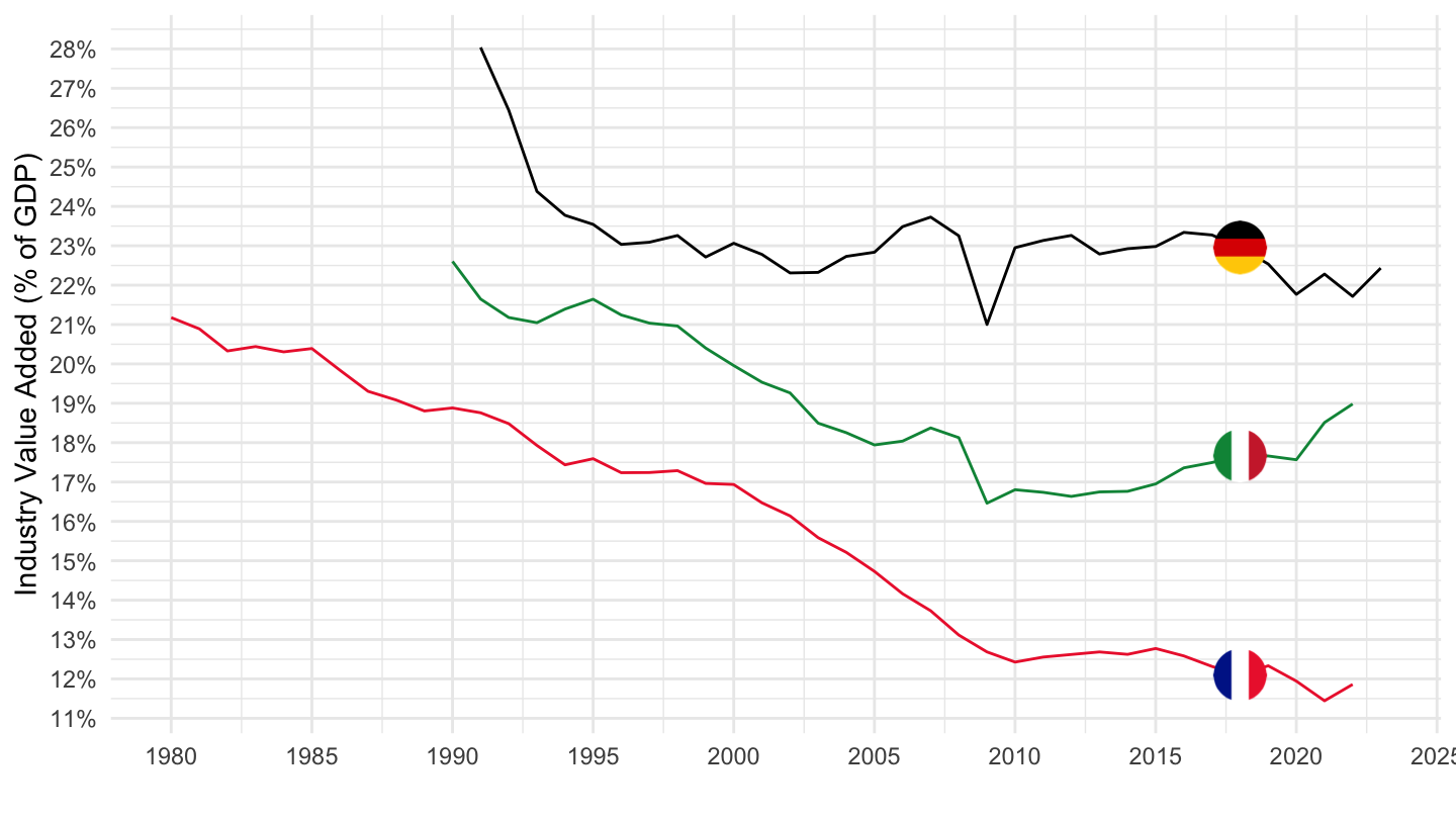
Australia, Eurozone, Japan
Code
SNA_TABLE1 %>%
  filter(LOCATION %in% c("AUS", "JPN", "EA19"),
         MEASURE == "C",
         TRANSACT %in% c("B1_GE", "B1GVB_E")) %>%
  year_to_date %>%
  filter(date >= as.Date("1994-01-01"),
         date <= as.Date("2020-01-01")) %>%
  left_join(SNA_TABLE1_var$LOCATION, by = "LOCATION") %>%
  select(date, Location, LOCATION, TRANSACT, obsValue) %>%
  spread(TRANSACT, obsValue) %>%
  mutate(obsValue = B1GVB_E / B1_GE) %>%
  mutate(Location = ifelse(LOCATION == "EA19", "Europe", Location)) %>%
  left_join(colors, by = c("Location" = "country")) %>%
  ggplot() + geom_line(aes(x = date, y = obsValue, color = color)) +
  ylab("Industry Value Added (% of GDP)") + xlab("") +
  scale_color_identity() + theme_minimal() + add_3flags +
  scale_x_date(breaks = seq(1920, 2100, 5) %>% paste0("-01-01") %>% as.Date,
               labels = date_format("%Y")) +
  scale_y_continuous(breaks = 0.01*seq(-60, 60, 1),
                     labels = scales::percent_format(accuracy = 1))
France, Germany, United States
Code
SNA_TABLE1 %>%
  filter(LOCATION %in% c("FRA", "DEU", "USA"),
         MEASURE == "C",
         TRANSACT %in% c("B1_GE", "B1GVB_E")) %>%
  year_to_date %>%
  filter(date >= as.Date("1994-01-01"),
         date <= as.Date("2020-01-01")) %>%
  left_join(SNA_TABLE1_var$LOCATION, by = "LOCATION") %>%
  select(date, Location, TRANSACT, obsValue) %>%
  spread(TRANSACT, obsValue) %>%
  mutate(B1GVB_E_B1_GE = B1GVB_E / B1_GE,
         Location = case_when(Location == "Germany" ~ "Allemagne",
                                   Location == "United States" ~ "Etats-Unis",
                                   Location == "France" ~ "France")) %>%
  ggplot() + geom_line() +
  aes(x = date, y = B1GVB_E_B1_GE, color = Location) +
  scale_color_manual(values = viridis(4)[1:3]) +
  theme_minimal() +
  scale_x_date(breaks = seq(1920, 2100, 2) %>% paste0("-01-01") %>% as.Date,
               labels = date_format("%Y")) +
  theme(legend.position = c(0.15, 0.2),
        legend.title = element_blank()) +
  scale_y_continuous(breaks = 0.01*seq(-60, 60, 1),
                     labels = scales::percent_format(accuracy = 1)) +
  ylab("Valeur Ajoutée dans l'Industrie (% du PIB)") + xlab("")
France, Germany, EA19
Code
SNA_TABLE1 %>%
  filter(LOCATION %in% c("FRA", "DEU", "EA19"),
         MEASURE == "C",
         TRANSACT %in% c("B1_GE", "B1GVB_E")) %>%
  year_to_date %>%
  filter(date >= as.Date("1994-01-01"),
         date <= as.Date("2020-01-01")) %>%
  left_join(SNA_TABLE1_var$LOCATION, by = "LOCATION") %>%
  select(date, Location, TRANSACT, obsValue) %>%
  spread(TRANSACT, obsValue) %>%
  mutate(B1GVB_E_B1_GE = B1GVB_E / B1_GE,
         Location = case_when(Location == "Germany" ~ "Allemagne",
                                   Location == "United States" ~ "Etats-Unis",
                                   Location == "France" ~ "France")) %>%
  ggplot() + geom_line() +
  aes(x = date, y = B1GVB_E_B1_GE, color = Location) +
  scale_color_manual(values = viridis(4)[1:3]) +
  theme_minimal() +
  scale_x_date(breaks = seq(1920, 2100, 2) %>% paste0("-01-01") %>% as.Date,
               labels = date_format("%Y")) +
  theme(legend.position = c(0.15, 0.2),
        legend.title = element_blank()) +
  scale_y_continuous(breaks = 0.01*seq(-60, 60, 1),
                     labels = scales::percent_format(accuracy = 1)) +
  ylab("Valeur Ajoutée dans l'Industrie (% du PIB)") + xlab("")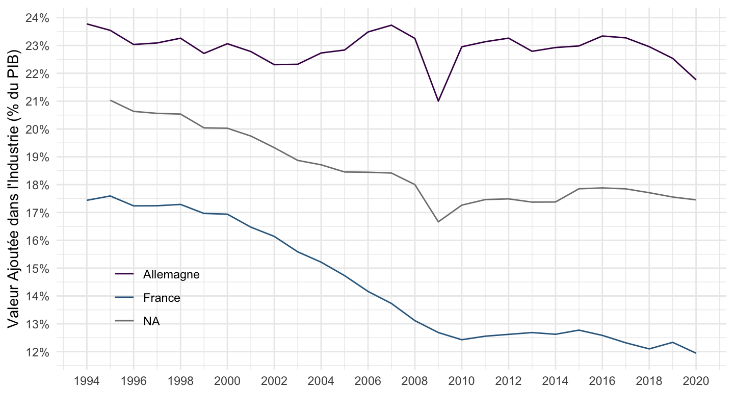
France, Germany, Italy
Code
SNA_TABLE1 %>%
  filter(LOCATION %in% c("FRA", "ITA", "DEU"),
         MEASURE == "C",
         TRANSACT %in% c("B1_GE", "B1GVB_E")) %>%
  year_to_date %>%
  filter(date >= as.Date("1994-01-01"),
         date <= as.Date("2020-01-01")) %>%
  left_join(SNA_TABLE1_var$LOCATION, by = "LOCATION") %>%
  select(date, Location, TRANSACT, obsValue) %>%
  spread(TRANSACT, obsValue) %>%
  mutate(obsValue = B1GVB_E / B1_GE) %>%
  left_join(colors, by = c("Location" = "country")) %>%
  ggplot() + geom_line(aes(x = date, y = obsValue, color = color)) +
  ylab("Industry Value Added (% of GDP)") + xlab("") +
  scale_color_identity() + theme_minimal() + add_3flags +
  scale_x_date(breaks = seq(1920, 2100, 5) %>% paste0("-01-01") %>% as.Date,
               labels = date_format("%Y")) +
  scale_y_continuous(breaks = 0.01*seq(-60, 60, 1),
                     labels = scales::percent_format(accuracy = 1))
France, Italy, Spain
Code
SNA_TABLE1 %>%
  filter(LOCATION %in% c("FRA", "ITA", "ESP"),
         MEASURE == "C",
         TRANSACT %in% c("B1_GE", "B1GVB_E")) %>%
  year_to_date %>%
  filter(date >= as.Date("1994-01-01"),
         date <= as.Date("2020-01-01")) %>%
  left_join(SNA_TABLE1_var$LOCATION, by = "LOCATION") %>%
  select(date, Location, TRANSACT, obsValue) %>%
  spread(TRANSACT, obsValue) %>%
  mutate(obsValue = B1GVB_E / B1_GE) %>%
  left_join(colors, by = c("Location" = "country")) %>%
  ggplot() + geom_line(aes(x = date, y = obsValue, color = color)) +
  ylab("Industry Value Added (% of GDP)") + xlab("") +
  scale_color_identity() + theme_minimal() + add_3flags +
  scale_x_date(breaks = seq(1920, 2100, 5) %>% paste0("-01-01") %>% as.Date,
               labels = date_format("%Y")) +
  scale_y_continuous(breaks = 0.01*seq(-60, 60, 1),
                     labels = scales::percent_format(accuracy = 1))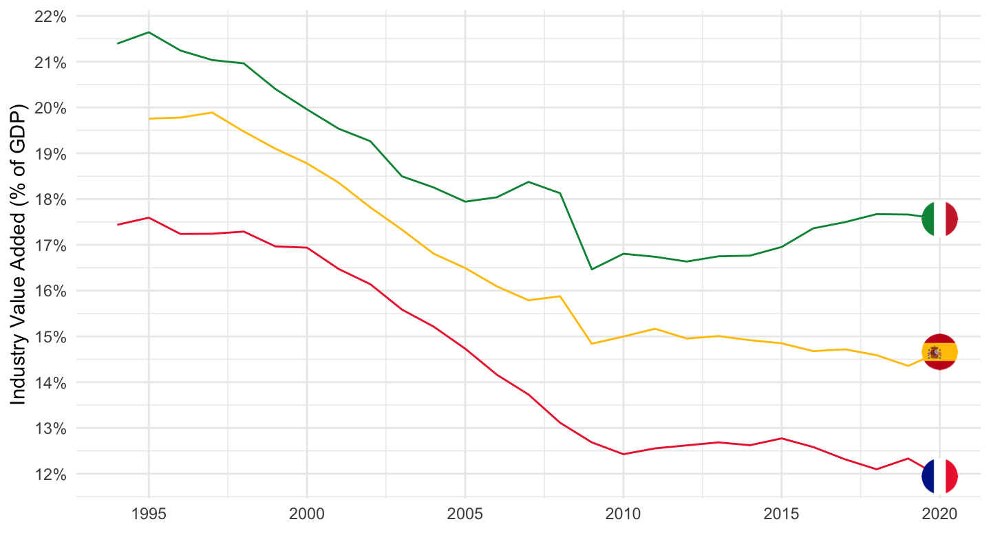
France, Allemagne, Italie
Code
SNA_TABLE1 %>%
  filter(LOCATION %in% c("FRA", "ITA", "DEU"),
         MEASURE == "C",
         TRANSACT %in% c("B1_GE", "B1GVC")) %>%
  year_to_date %>%
  filter(date >= as.Date("1994-01-01"),
         date <= as.Date("2020-01-01")) %>%
  left_join(SNA_TABLE1_var$LOCATION, by = "LOCATION") %>%
  select(date, Location, TRANSACT, obsValue) %>%
  spread(TRANSACT, obsValue) %>%
  mutate(B1GVC_B1_GE = B1GVC / B1_GE,
         Location = case_when(Location == "Germany" ~ "Allemagne",
                                   Location == "Italy" ~ "Italie",
                                   Location == "France" ~ "France")) %>%
  ggplot() + geom_line() +
  aes(x = date, y = B1GVC_B1_GE, color = Location) +
  scale_color_manual(values = viridis(4)[1:3]) +
  theme_minimal() +
  scale_x_date(breaks = seq(1920, 2100, 2) %>% paste0("-01-01") %>% as.Date,
               labels = date_format("%Y")) +
  theme(legend.position = c(0.15, 0.2),
        legend.title = element_blank()) +
  scale_y_continuous(breaks = 0.01*seq(-60, 60, 1),
                     labels = scales::percent_format(accuracy = 1)) +
  ylab("Valeur Ajoutée dans l'Industrie (% du PIB)") + xlab("")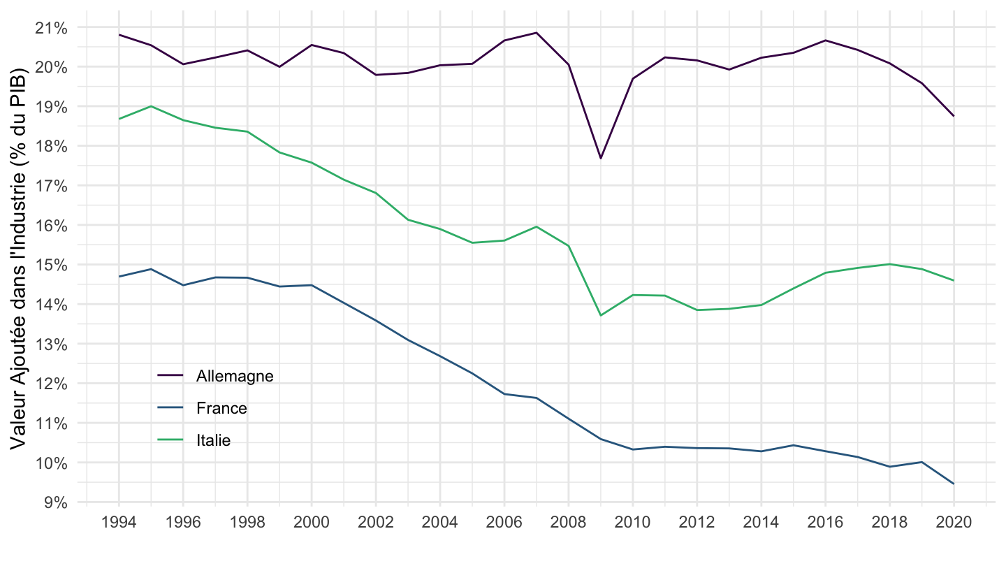
D11VC - Manufacturing Wages and Salaries (without contributions)
Code
SNA_TABLE1 %>%
  filter(LOCATION %in% c("FRA", "ITA", "DEU"),
         MEASURE == "C",
         TRANSACT %in% c("B1_GE", "D11VC")) %>%
  year_to_date %>%
  filter(date >= as.Date("1980-01-01")) %>%
  left_join(SNA_TABLE1_var$LOCATION, by = "LOCATION") %>%
  select(date, Location, TRANSACT, obsValue) %>%
  spread(TRANSACT, obsValue) %>%
  mutate(D11VC_B1_GE = D11VC / B1_GE) %>%
  ggplot() + geom_line() +
  aes(x = date, y = D11VC_B1_GE, color = Location) +
  scale_color_manual(values = viridis(4)[1:3]) +
  theme_minimal() +
  scale_x_date(breaks = seq(1920, 2100, 5) %>% paste0("-01-01") %>% as.Date,
               labels = date_format("%Y")) +
  theme(legend.position = c(0.15, 0.2),
        legend.title = element_blank()) +
  scale_y_continuous(breaks = 0.01*seq(-60, 60, 1),
                     labels = scales::percent_format(accuracy = 1)) +
  ylab("Manufacturing Wages (% of GDP)") + xlab("")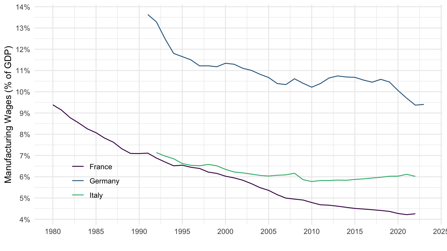
D1VC - Manufacturing Compensation of Employees (with contributions)
Code
SNA_TABLE1 %>%
  filter(LOCATION %in% c("FRA", "ITA", "DEU"),
         MEASURE == "C",
         TRANSACT %in% c("B1_GE", "D1VC")) %>%
  year_to_date %>%
  filter(date >= as.Date("1980-01-01")) %>%
  left_join(SNA_TABLE1_var$LOCATION, by = "LOCATION") %>%
  select(date, Location, TRANSACT, obsValue) %>%
  spread(TRANSACT, obsValue) %>%
  mutate(value = D1VC / B1_GE) %>%
  ggplot() + geom_line() +
  aes(x = date, y = value, color = Location) +
  scale_color_manual(values = viridis(4)[1:3]) +
  theme_minimal() +
  scale_x_date(breaks = seq(1920, 2100, 5) %>% paste0("-01-01") %>% as.Date,
               labels = date_format("%Y")) +
  theme(legend.position = c(0.15, 0.2),
        legend.title = element_blank()) +
  scale_y_continuous(breaks = 0.01*seq(-60, 60, 1),
                     labels = scales::percent_format(accuracy = 1)) +
  ylab("Manufacturing Compensation of Employees (% of GDP)") + xlab("")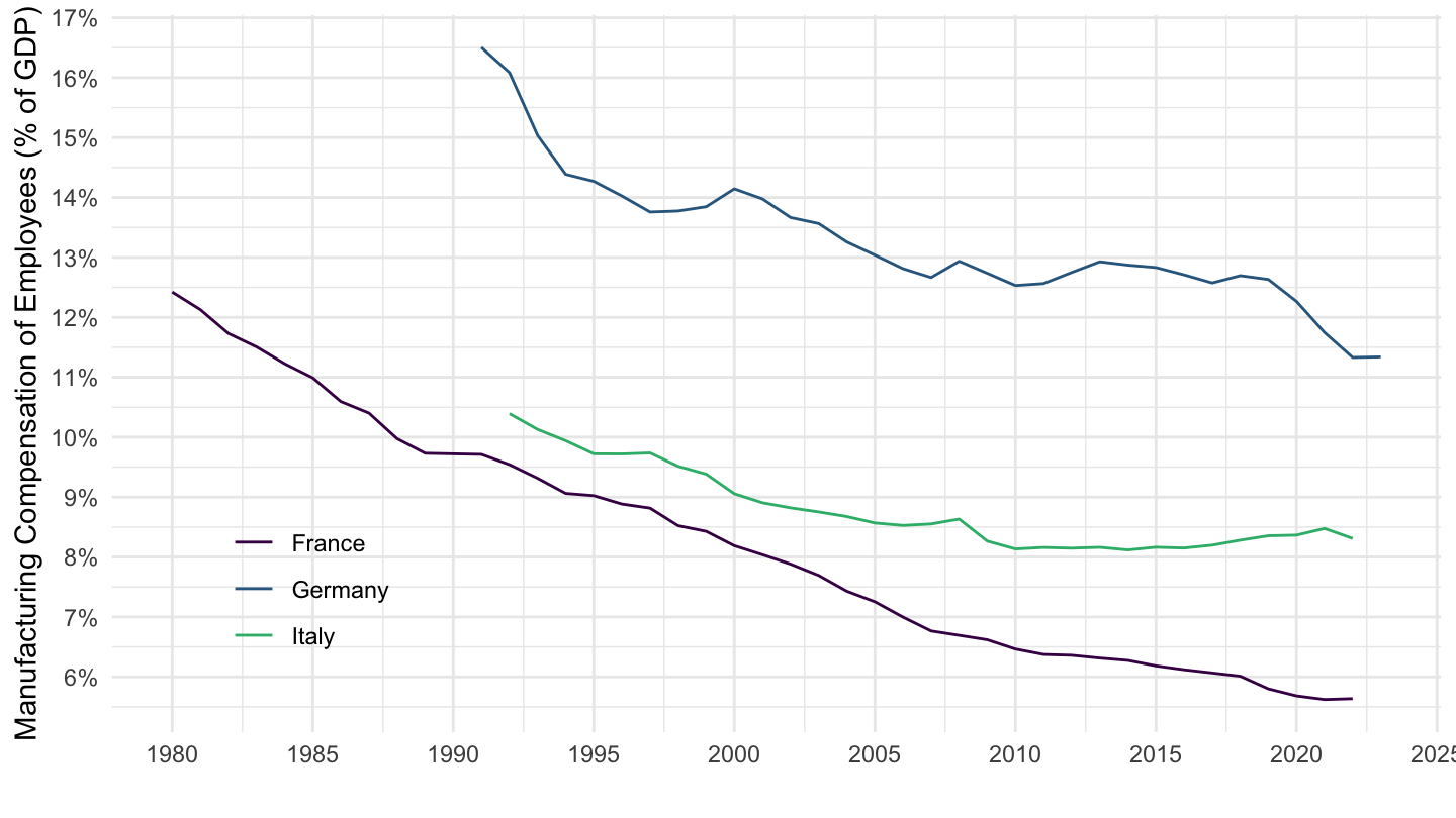
B1_GA - Gross domestic product (output approach)
Code
SNA_TABLE1 %>%
  filter(LOCATION %in% c("USA"),
         TRANSACT == "B1_GA",
         MEASURE %in% c("C", "V")) %>%
  mutate(date = paste0(obsTime, "-01-01") %>% as.Date,
         obsValue = obsValue / 10^6) %>%
  left_join(SNA_TABLE1_var$LOCATION, by = "LOCATION") %>%
  left_join(SNA_TABLE1_var$MEASURE, by = "MEASURE") %>%
  group_by(LOCATION) %>%
  arrange(date) %>%
  select(date, obsValue, Measure) %>%
  ggplot(.) + geom_line(aes(x = date, y = obsValue, linetype = Measure, color = Measure)) +
  theme_minimal() + xlab("") + ylab("") +
  scale_color_manual(values = viridis(4)[1:3]) +
  geom_rect(data = nber_recessions,
            aes(xmin = Peak, xmax = Trough, ymin = -Inf, ymax = +Inf),
            fill = 'grey', alpha = 0.5) +
  scale_x_date(breaks = seq(1960, 2100, 5) %>% paste0("-01-01") %>% as.Date,
               labels = date_format("%Y"),
               limits = c(1970, 2019) %>% paste0("-01-01") %>% as.Date) +
  scale_y_continuous(breaks = seq(0, 30, 1),
                     labels = dollar_format(suffix = "Tn", prefix = "$", accuracy = 1)) +
  theme(legend.position = c(0.3, 0.90),
        legend.title = element_blank())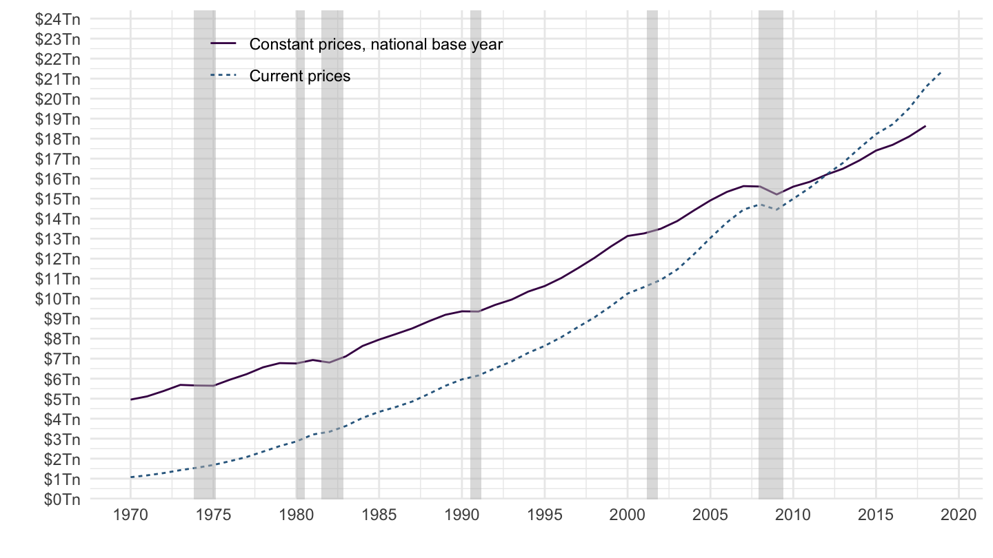
P3 - Final consumption expenditure
Code
SNA_TABLE1 %>%
  filter(LOCATION %in% c("USA"),
         TRANSACT == "P3",
         MEASURE %in% c("C", "V")) %>%
  mutate(date = paste0(obsTime, "-01-01") %>% as.Date,
         obsValue = obsValue / 10^6) %>%
  left_join(SNA_TABLE1_var$LOCATION, by = "LOCATION") %>%
  left_join(SNA_TABLE1_var$MEASURE, by = "MEASURE") %>%
  group_by(LOCATION) %>%
  arrange(date) %>%
  select(date, obsValue, Measure) %>%
  ggplot(.) +
  geom_line(aes(x = date, y = obsValue, linetype = Measure, color = Measure)) +
  theme_minimal() + xlab("") + ylab("") +
  scale_color_manual(values = viridis(4)[1:3]) +
  geom_rect(data = nber_recessions,
            aes(xmin = Peak, xmax = Trough, ymin = -Inf, ymax = +Inf),
            fill = 'grey', alpha = 0.5) +
  scale_x_date(breaks = seq(1960, 2100, 5) %>% paste0("-01-01") %>% as.Date,
               labels = date_format("%Y"),
               limits = c(1970, 2019) %>% paste0("-01-01") %>% as.Date) +
  scale_y_continuous(breaks = seq(0, 30, 1),
                     labels = dollar_format(suffix = "Tn", prefix = "$", accuracy = 1)) +
  theme(legend.position = c(0.3, 0.90),
        legend.title = element_blank())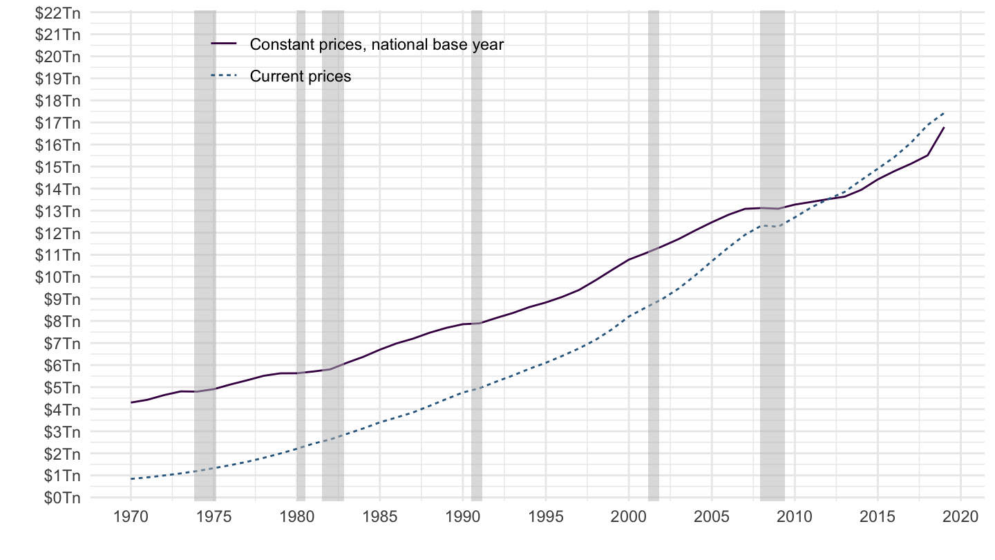
Individual Consumption / trend GDP
France, Germany, Italy
Code
SNA_TABLE1 %>%
  filter(MEASURE == "VXVOB",
         LOCATION %in% c("FRA", "DEU", "ITA"),
         TRANSACT %in% c("B1_GE", "P41")) %>%
  year_to_date %>%
  left_join(SNA_TABLE1_var$LOCATION %>%
              setNames(c("LOCATION", "Location")), by = "LOCATION") %>%
  select(Location, date, TRANSACT, obsValue) %>%
  spread(TRANSACT, obsValue) %>%
  group_by(Location) %>%
  mutate(B1_GE_trend = log(B1_GE) %>% hpfilter(1000000) %>% pluck("trend") %>% exp,
         P41_B1_GE_trend = P41 / B1_GE_trend,
         P41_B1_GE = P41 / B1_GE) %>%
  select(Location, date, P41_B1_GE_trend) %>%
  na.omit %>%
  ggplot() + geom_line(aes(x = date, y = P41_B1_GE_trend, color = Location)) +
  scale_color_manual(values = c("#0055a4", "#000000", "#008c45")) +
  theme_minimal() +
  scale_x_date(breaks = seq(1920, 2100, 10) %>% paste0("-01-01") %>% as.Date,
               labels = date_format("%Y")) +
  theme(legend.position = c(0.15, 0.9),
        legend.title = element_blank()) +
  scale_y_continuous(breaks = 0.01*seq(-10, 100, 5),
                     labels = scales::percent_format(accuracy = 1)) +
  ylab("Individual Consumption (% of trend GDP)") + xlab("")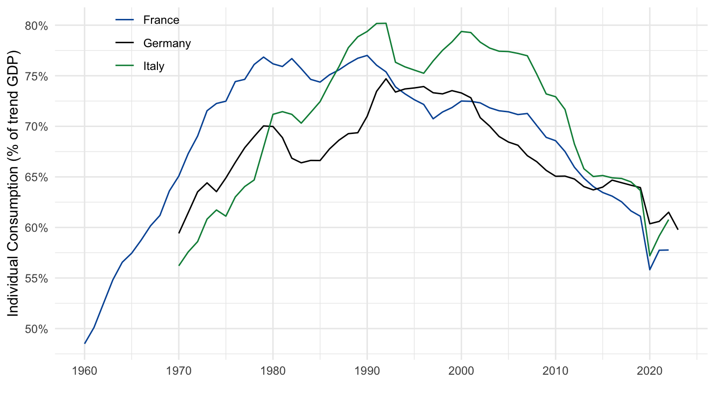
United Kingdom, Japan, United States
Code
SNA_TABLE1 %>%
  filter(MEASURE == "VXVOB",
         LOCATION %in% c("JPN", "GBR", "USA"),
         TRANSACT %in% c("B1_GE", "P41")) %>%
  year_to_date %>%
  left_join(SNA_TABLE1_var$LOCATION %>%
              setNames(c("LOCATION", "Location")), by = "LOCATION") %>%
  select(Location, date, TRANSACT, obsValue) %>%
  spread(TRANSACT, obsValue) %>%
  group_by(Location) %>%
  mutate(B1_GE_trend = log(B1_GE) %>% hpfilter(100000) %>% pluck("trend") %>% exp,
         P41_B1_GE_trend = P41 / B1_GE_trend,
         P41_B1_GE = P41 / B1_GE) %>%
  select(Location, date, P41_B1_GE_trend) %>%
  na.omit %>%
  ggplot() + geom_line(aes(x = date, y = P41_B1_GE_trend, color = Location)) +
  scale_color_manual(values = viridis(4)[1:3]) +
  theme_minimal() +
  scale_x_date(breaks = seq(1920, 2100, 10) %>% paste0("-01-01") %>% as.Date,
               labels = date_format("%Y")) +
  theme(legend.position = c(0.15, 0.9),
        legend.title = element_blank()) +
  scale_y_continuous(breaks = 0.01*seq(-10, 100, 5),
                     labels = scales::percent_format(accuracy = 1)) +
  ylab("Individual Consumption (% of trend GDP)") + xlab("")
Switzerland, Germany, Netherlands
Code
SNA_TABLE1 %>%
  filter(MEASURE == "VXVOB",
         LOCATION %in% c("NLD", "CHE", "DEU"),
         TRANSACT %in% c("B1_GE", "P41")) %>%
  year_to_date %>%
  left_join(SNA_TABLE1_var$LOCATION %>%
              setNames(c("LOCATION", "Location")), by = "LOCATION") %>%
  select(Location, date, TRANSACT, obsValue) %>%
  spread(TRANSACT, obsValue) %>%
  group_by(Location) %>%
  mutate(B1_GE_trend = log(B1_GE) %>% hpfilter(100000) %>% pluck("trend") %>% exp,
         P41_B1_GE_trend = P41 / B1_GE_trend,
         P41_B1_GE = P41 / B1_GE) %>%
  select(Location, date, P41_B1_GE_trend) %>%
  na.omit %>%
  ggplot() + geom_line(aes(x = date, y = P41_B1_GE_trend, color = Location)) +
  scale_color_manual(values = viridis(4)[1:3]) +
  theme_minimal() +
  scale_x_date(breaks = seq(1920, 2100, 10) %>% paste0("-01-01") %>% as.Date,
               labels = date_format("%Y")) +
  theme(legend.position = c(0.85, 0.8),
        legend.title = element_blank()) +
  scale_y_continuous(breaks = 0.01*seq(-10, 100, 2),
                     labels = scales::percent_format(accuracy = 1)) +
  ylab("Individual Consumption (% of trend GDP)") + xlab("")
Net Exports / trend GDP
France, Germany, Italy
Code
SNA_TABLE1 %>%
  filter(MEASURE == "VXVOB",
         LOCATION %in% c("FRA", "DEU", "ITA"),
         TRANSACT %in% c("B1_GE", "B11")) %>%
  year_to_date %>%
  left_join(SNA_TABLE1_var$LOCATION, by = "LOCATION") %>%
  select(Location, date, TRANSACT, obsValue) %>%
  spread(TRANSACT, obsValue) %>%
  group_by(Location) %>%
  mutate(B1_GE_trend = log(B1_GE) %>% hpfilter(1000000) %>% pluck("trend") %>% exp,
         B11_B1_GE_trend = B11 / B1_GE_trend,
         B11_B1_GE = B11 / B1_GE) %>%
  select(Location, date, B11_B1_GE_trend) %>%
  na.omit %>%
  ggplot() + geom_line() + theme_minimal() +
  aes(x = date, y = B11_B1_GE_trend, color = Location) +
  scale_color_manual(values = c("#0055a4", "#000000", "#008c45")) +
  scale_x_date(breaks = seq(1920, 2100, 10) %>% paste0("-01-01") %>% as.Date,
               labels = date_format("%Y")) +
  theme(legend.position = c(0.15, 0.9),
        legend.title = element_blank()) +
  scale_y_continuous(breaks = 0.01*seq(-10, 100, 1),
                     labels = scales::percent_format(accuracy = 1)) +
  ylab("External balance (% of trend GDP)") + xlab("")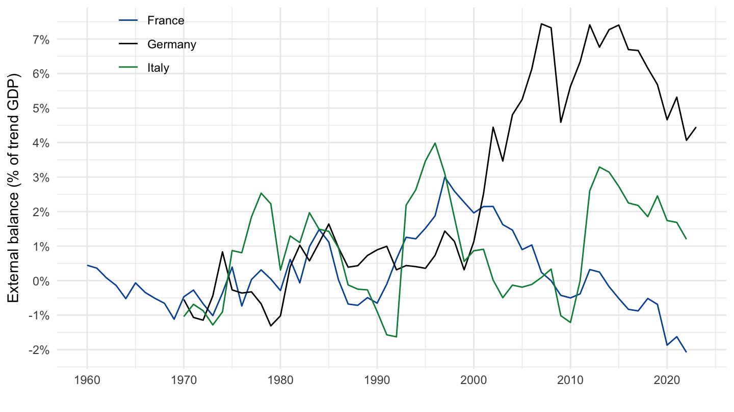
Austria, Finland, New Zealand
Code
SNA_TABLE1 %>%
  filter(MEASURE == "VXVOB",
         LOCATION %in% c("AUS", "FIN", "NLZ"),
         TRANSACT %in% c("B1_GE", "B11")) %>%
  year_to_date %>%
  left_join(SNA_TABLE1_var$LOCATION %>%
              setNames(c("LOCATION", "Location")), by = "LOCATION") %>%
  select(Location, date, TRANSACT, obsValue) %>%
  spread(TRANSACT, obsValue) %>%
  group_by(Location) %>%
  mutate(B1_GE_trend = log(B1_GE) %>% hpfilter(1000000) %>% pluck("trend") %>% exp,
         B11_B1_GE_trend = B11 / B1_GE_trend,
         B11_B1_GE = B11 / B1_GE) %>%
  select(Location, date, B11_B1_GE_trend) %>%
  na.omit %>%
  ggplot() + geom_line(aes(x = date, y = B11_B1_GE_trend, color = Location)) +
  scale_color_manual(values = viridis(4)[1:3]) +
  theme_minimal() +
  scale_x_date(breaks = seq(1920, 2100, 10) %>% paste0("-01-01") %>% as.Date,
               labels = date_format("%Y")) +
  theme(legend.position = c(0.15, 0.9),
        legend.title = element_blank()) +
  scale_y_continuous(breaks = 0.01*seq(-10, 100, 1),
                     labels = scales::percent_format(accuracy = 1)) +
  ylab("External balance (% of trend GDP)") + xlab("")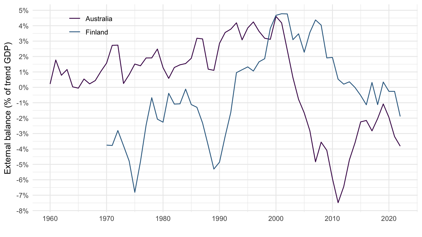
United Kingdom, Japan, United States
Code
SNA_TABLE1 %>%
  filter(MEASURE == "VXVOB",
         LOCATION %in% c("JPN", "GBR", "USA"),
         TRANSACT %in% c("B1_GE", "B11")) %>%
  year_to_date %>%
  left_join(SNA_TABLE1_var$LOCATION %>%
              setNames(c("LOCATION", "Location")), by = "LOCATION") %>%
  select(Location, date, TRANSACT, obsValue) %>%
  spread(TRANSACT, obsValue) %>%
  group_by(Location) %>%
  mutate(B1_GE_trend = log(B1_GE) %>% hpfilter(100000) %>% pluck("trend") %>% exp,
         B11_B1_GE_trend = B11 / B1_GE_trend,
         B11_B1_GE = B11 / B1_GE) %>%
  select(Location, date, B11_B1_GE_trend) %>%
  na.omit %>%
  ggplot() + geom_line(aes(x = date, y = B11_B1_GE_trend, color = Location)) +
  scale_color_manual(values = viridis(4)[1:3]) +
  theme_minimal() +
  scale_x_date(breaks = seq(1920, 2100, 10) %>% paste0("-01-01") %>% as.Date,
               labels = date_format("%Y")) +
  theme(legend.position = c(0.85, 0.9),
        legend.title = element_blank()) +
  scale_y_continuous(breaks = 0.01*seq(-10, 100, 1),
                     labels = scales::percent_format(accuracy = 1)) +
  ylab("External balance (% of trend GDP)") + xlab("")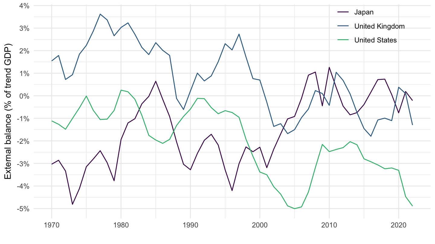
Switzerland, Germany, Netherlands
Code
SNA_TABLE1 %>%
  filter(MEASURE == "VXVOB",
         LOCATION %in% c("NLD", "CHE", "DEU"),
         TRANSACT %in% c("B1_GE", "B11")) %>%
  year_to_date %>%
  left_join(SNA_TABLE1_var$LOCATION %>%
              setNames(c("LOCATION", "Location")), by = "LOCATION") %>%
  select(Location, date, TRANSACT, obsValue) %>%
  spread(TRANSACT, obsValue) %>%
  group_by(Location) %>%
  mutate(B1_GE_trend = log(B1_GE) %>% hpfilter(100000) %>% pluck("trend") %>% exp,
         B11_B1_GE_trend = B11 / B1_GE_trend,
         B11_B1_GE = B11 / B1_GE) %>%
  select(Location, date, B11_B1_GE_trend) %>%
  na.omit %>%
  ggplot() + geom_line(aes(x = date, y = B11_B1_GE_trend, color = Location)) +
  scale_color_manual(values = viridis(4)[1:3]) +
  theme_minimal() +
  scale_x_date(breaks = seq(1920, 2100, 10) %>% paste0("-01-01") %>% as.Date,
               labels = date_format("%Y")) +
  theme(legend.position = c(0.15, 0.8),
        legend.title = element_blank()) +
  scale_y_continuous(breaks = 0.01*seq(-10, 100, 2),
                     labels = scales::percent_format(accuracy = 1)) +
  ylab("External balance (% of trend GDP)") + xlab("")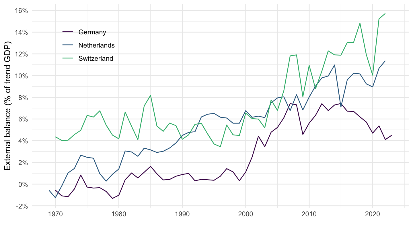
Chile, Denmark, Sweden
Code
SNA_TABLE1 %>%
  filter(MEASURE == "VXVOB",
         LOCATION %in% c("SWE", "DNK", "CHL"),
         TRANSACT %in% c("B1_GE", "B11")) %>%
  year_to_date %>%
  left_join(SNA_TABLE1_var$LOCATION %>%
              setNames(c("LOCATION", "Location")), by = "LOCATION") %>%
  select(Location, date, TRANSACT, obsValue) %>%
  spread(TRANSACT, obsValue) %>%
  group_by(Location) %>%
  mutate(B1_GE_trend = log(B1_GE) %>% hpfilter(1000000) %>% pluck("trend") %>% exp,
         B11_B1_GE_trend = B11 / B1_GE_trend,
         B11_B1_GE = B11 / B1_GE) %>%
  select(Location, date, B11_B1_GE_trend) %>%
  na.omit %>%
  ggplot() + geom_line(aes(x = date, y = B11_B1_GE_trend, color = Location)) +
  scale_color_manual(values = viridis(4)[1:3]) +
  theme_minimal() +
  scale_x_date(breaks = seq(1920, 2100, 10) %>% paste0("-01-01") %>% as.Date,
               labels = date_format("%Y")) +
  theme(legend.position = c(0.15, 0.8),
        legend.title = element_blank()) +
  scale_y_continuous(breaks = 0.01*seq(-10, 100, 1),
                     labels = scales::percent_format(accuracy = 1)) +
  ylab("External balance (% of trend GDP)") + xlab("")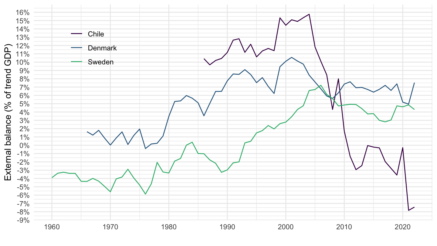
Argentina, Brazil, Chile
Code
SNA_TABLE1 %>%
  filter(MEASURE == "VXVOB",
         LOCATION %in% c("ARG", "BRA", "CHL"),
         TRANSACT %in% c("B1_GE", "B11")) %>%
  year_to_date %>%
  left_join(SNA_TABLE1_var$LOCATION %>%
              setNames(c("LOCATION", "Location")), by = "LOCATION") %>%
  select(Location, date, TRANSACT, obsValue) %>%
  spread(TRANSACT, obsValue) %>%
  group_by(Location) %>%
  mutate(B1_GE_trend = log(B1_GE) %>% hpfilter(1000000) %>% pluck("trend") %>% exp,
         B11_B1_GE_trend = B11 / B1_GE_trend,
         B11_B1_GE = B11 / B1_GE) %>%
  select(Location, date, B11_B1_GE_trend) %>%
  na.omit %>%
  ggplot() + geom_line(aes(x = date, y = B11_B1_GE_trend, color = Location)) +
  scale_color_manual(values = viridis(4)[1:3]) +
  theme_minimal() +
  scale_x_date(breaks = seq(1920, 2100, 10) %>% paste0("-01-01") %>% as.Date,
               labels = date_format("%Y")) +
  theme(legend.position = c(0.15, 0.2),
        legend.title = element_blank()) +
  scale_y_continuous(breaks = 0.01*seq(-10, 100, 1),
                     labels = scales::percent_format(accuracy = 1)) +
  ylab("External balance (% of trend GDP)") + xlab("")
Consumption / trend GDP
France, Germany, Italy
Code
SNA_TABLE1 %>%
  filter(MEASURE == "VXVOB",
         LOCATION %in% c("FRA", "DEU", "ITA"),
         TRANSACT %in% c("B1_GE", "P31S14")) %>%
  year_to_date %>%
  left_join(SNA_TABLE1_var$LOCATION %>%
              setNames(c("LOCATION", "Location")), by = "LOCATION") %>%
  select(Location, date, TRANSACT, obsValue) %>%
  spread(TRANSACT, obsValue) %>%
  group_by(Location) %>%
  mutate(B1_GE_trend = log(B1_GE) %>% hpfilter(1000000) %>% pluck("trend") %>% exp,
         P31S14_B1_GE_trend = P31S14 / B1_GE_trend,
         P31S14_B1_GE = P31S14 / B1_GE) %>%
  select(Location, date, P31S14_B1_GE_trend) %>%
  na.omit %>%
  ggplot() + geom_line(aes(x = date, y = P31S14_B1_GE_trend, color = Location)) +
  scale_color_manual(values = viridis(4)[1:3]) +
  theme_minimal() +
  scale_x_date(breaks = seq(1920, 2100, 10) %>% paste0("-01-01") %>% as.Date,
               labels = date_format("%Y")) +
  theme(legend.position = c(0.15, 0.9),
        legend.title = element_blank()) +
  scale_y_continuous(breaks = 0.01*seq(0, 100, 5),
                     labels = scales::percent_format(accuracy = 1)) +
  ylab("External balance (% of trend GDP)") + xlab("")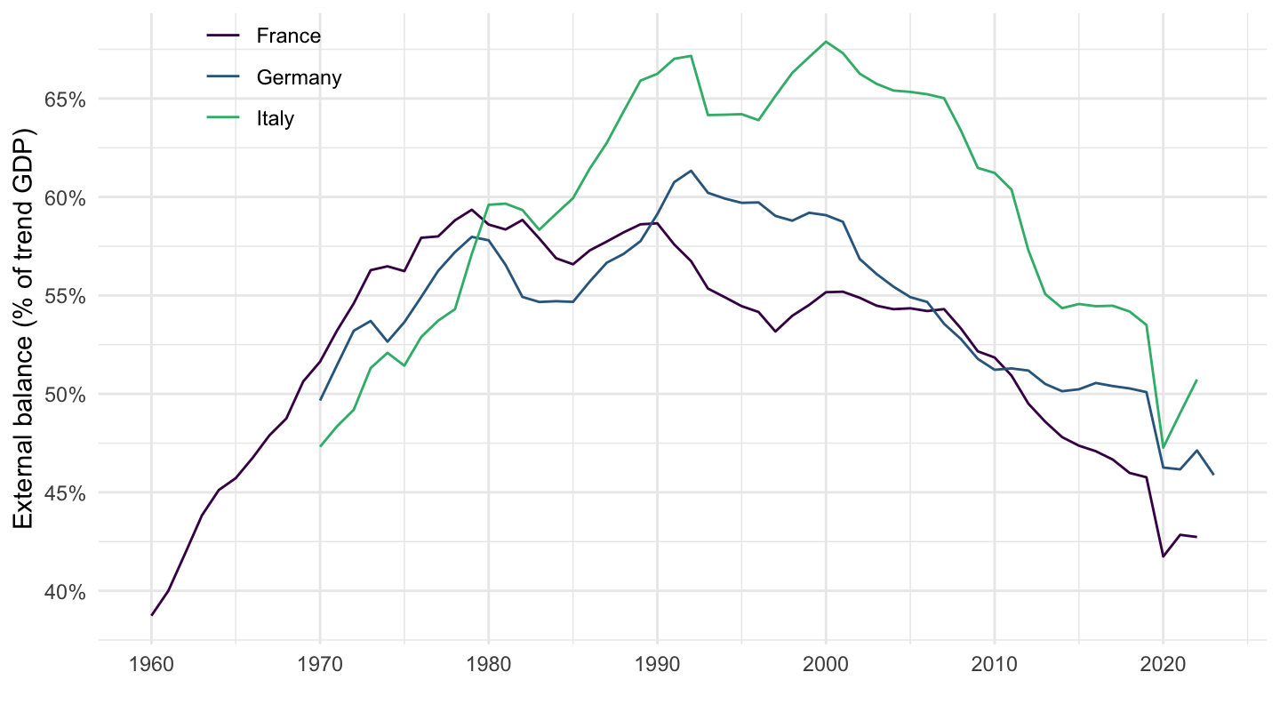
United Kingdom, Japan, United States
Code
SNA_TABLE1 %>%
  filter(MEASURE == "VXVOB",
         LOCATION %in% c("JPN", "GBR", "USA"),
         TRANSACT %in% c("B1_GE", "P31S14")) %>%
  year_to_date %>%
  left_join(SNA_TABLE1_var$LOCATION %>%
              setNames(c("LOCATION", "Location")), by = "LOCATION") %>%
  select(Location, date, TRANSACT, obsValue) %>%
  spread(TRANSACT, obsValue) %>%
  group_by(Location) %>%
  mutate(B1_GE_trend = log(B1_GE) %>% hpfilter(100000) %>% pluck("trend") %>% exp,
         P31S14_B1_GE_trend = P31S14 / B1_GE_trend,
         P31S14_B1_GE = P31S14 / B1_GE) %>%
  select(Location, date, P31S14_B1_GE_trend) %>%
  na.omit %>%
  ggplot() + geom_line(aes(x = date, y = P31S14_B1_GE_trend, color = Location)) +
  scale_color_manual(values = viridis(4)[1:3]) +
  theme_minimal() +
  scale_x_date(breaks = seq(1920, 2100, 10) %>% paste0("-01-01") %>% as.Date,
               labels = date_format("%Y")) +
  theme(legend.position = c(0.15, 0.9),
        legend.title = element_blank()) +
  scale_y_continuous(breaks = 0.01*seq(0, 100, 5),
                     labels = scales::percent_format(accuracy = 1)) +
  ylab("Consumption (% of trend GDP)") + xlab("")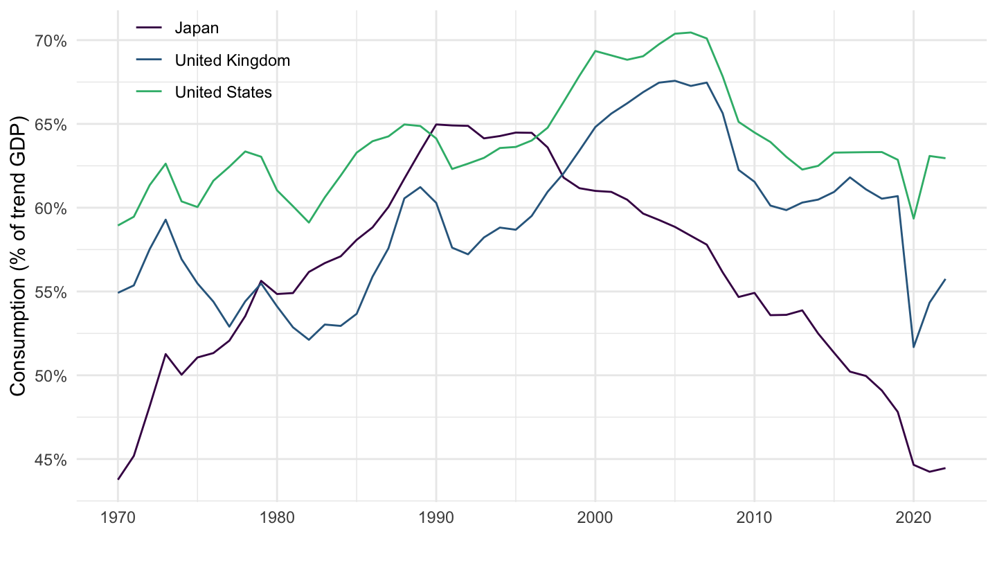
Switzerland, Germany, Netherlands
Code
SNA_TABLE1 %>%
  filter(MEASURE == "VXVOB",
         LOCATION %in% c("NLD", "CHE", "DEU"),
         TRANSACT %in% c("B1_GE", "P31S14")) %>%
  year_to_date %>%
  left_join(SNA_TABLE1_var$LOCATION %>%
              setNames(c("LOCATION", "Location")), by = "LOCATION") %>%
  select(Location, date, TRANSACT, obsValue) %>%
  spread(TRANSACT, obsValue) %>%
  group_by(Location) %>%
  mutate(B1_GE_trend = log(B1_GE) %>% hpfilter(100000) %>% pluck("trend") %>% exp,
         P31S14_B1_GE_trend = P31S14 / B1_GE_trend,
         P31S14_B1_GE = P31S14 / B1_GE) %>%
  select(Location, date, P31S14_B1_GE_trend) %>%
  na.omit %>%
  ggplot() + geom_line(aes(x = date, y = P31S14_B1_GE_trend, color = Location)) +
  scale_color_manual(values = viridis(4)[1:3]) +
  theme_minimal() +
  scale_x_date(breaks = seq(1920, 2100, 10) %>% paste0("-01-01") %>% as.Date,
               labels = date_format("%Y")) +
  theme(legend.position = c(0.15, 0.3),
        legend.title = element_blank()) +
  scale_y_continuous(breaks = 0.01*seq(0, 100, 5),
                     labels = scales::percent_format(accuracy = 1)) +
  ylab("Consumption (% of trend GDP)") + xlab("")
Government Spending / trend GDP
France, Germany, Italy
Code
SNA_TABLE1 %>%
  filter(MEASURE == "VXVOB",
         LOCATION %in% c("FRA", "DEU", "ITA"),
         TRANSACT %in% c("B1_GE", "P3S13")) %>%
  year_to_date %>%
  left_join(SNA_TABLE1_var$LOCATION %>%
              setNames(c("LOCATION", "Location")), by = "LOCATION") %>%
  select(Location, date, TRANSACT, obsValue) %>%
  spread(TRANSACT, obsValue) %>%
  group_by(Location) %>%
  mutate(B1_GE_trend = log(B1_GE) %>% hpfilter(1000000) %>% pluck("trend") %>% exp,
         P3S13_B1_GE_trend = P3S13 / B1_GE_trend,
         P3S13_B1_GE = P3S13 / B1_GE) %>%
  select(Location, date, P3S13_B1_GE_trend) %>%
  na.omit %>%
  ggplot() + geom_line(aes(x = date, y = P3S13_B1_GE_trend, color = Location)) +
  scale_color_manual(values = viridis(4)[1:3]) +
  theme_minimal() +
  scale_x_date(breaks = seq(1920, 2100, 10) %>% paste0("-01-01") %>% as.Date,
               labels = date_format("%Y")) +
  theme(legend.position = c(0.15, 0.9),
        legend.title = element_blank()) +
  scale_y_continuous(breaks = 0.01*seq(0, 100, 1),
                     labels = scales::percent_format(accuracy = 1)) +
  ylab("Spending (% of trend GDP)") + xlab("")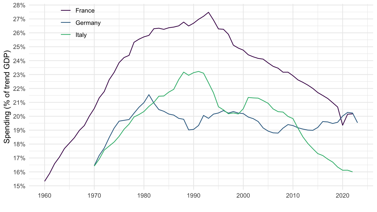
United Kingdom, Japan, United States
Code
SNA_TABLE1 %>%
  filter(MEASURE == "VXVOB",
         LOCATION %in% c("JPN", "GBR", "USA"),
         TRANSACT %in% c("B1_GE", "P3S13")) %>%
  year_to_date %>%
  left_join(SNA_TABLE1_var$LOCATION %>%
              setNames(c("LOCATION", "Location")), by = "LOCATION") %>%
  select(Location, date, TRANSACT, obsValue) %>%
  spread(TRANSACT, obsValue) %>%
  group_by(Location) %>%
  mutate(B1_GE_trend = log(B1_GE) %>% hpfilter(100000) %>% pluck("trend") %>% exp,
         P3S13_B1_GE_trend = P3S13 / B1_GE_trend,
         P3S13_B1_GE = P3S13 / B1_GE) %>%
  select(Location, date, P3S13_B1_GE_trend) %>%
  na.omit %>%
  ggplot() + geom_line(aes(x = date, y = P3S13_B1_GE_trend, color = Location)) +
  scale_color_manual(values = viridis(4)[1:3]) +
  theme_minimal() +
  scale_x_date(breaks = seq(1920, 2100, 10) %>% paste0("-01-01") %>% as.Date,
               labels = date_format("%Y")) +
  theme(legend.position = c(0.85, 0.9),
        legend.title = element_blank()) +
  scale_y_continuous(breaks = 0.01*seq(0, 100, 1),
                     labels = scales::percent_format(accuracy = 1)) +
  ylab("Government Spending (% of trend GDP)") + xlab("")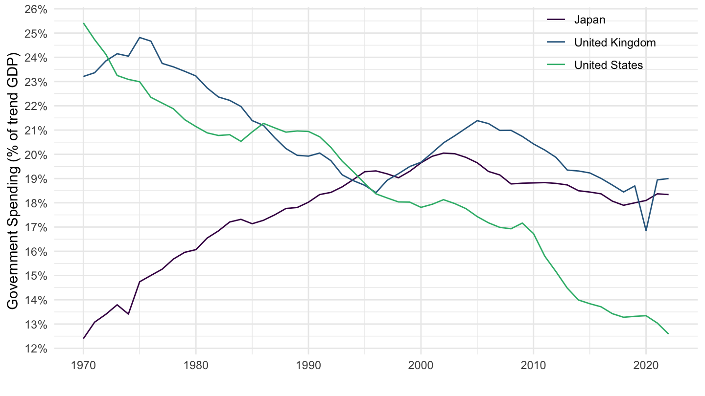
Switzerland, Germany, Netherlands
Code
SNA_TABLE1 %>%
  filter(MEASURE == "VXVOB",
         LOCATION %in% c("NLD", "CHE", "DEU"),
         TRANSACT %in% c("B1_GE", "P3S13")) %>%
  year_to_date %>%
  left_join(SNA_TABLE1_var$LOCATION %>%
              setNames(c("LOCATION", "Location")), by = "LOCATION") %>%
  select(Location, date, TRANSACT, obsValue) %>%
  spread(TRANSACT, obsValue) %>%
  group_by(Location) %>%
  mutate(B1_GE_trend = log(B1_GE) %>% hpfilter(100000) %>% pluck("trend") %>% exp,
         P3S13_B1_GE_trend = P3S13 / B1_GE_trend,
         P3S13_B1_GE = P3S13 / B1_GE) %>%
  select(Location, date, P3S13_B1_GE_trend) %>%
  na.omit %>%
  ggplot() + geom_line(aes(x = date, y = P3S13_B1_GE_trend, color = Location)) +
  scale_color_manual(values = viridis(4)[1:3]) +
  theme_minimal() +
  scale_x_date(breaks = seq(1920, 2100, 10) %>% paste0("-01-01") %>% as.Date,
               labels = date_format("%Y")) +
  theme(legend.position = c(0.15, 0.8),
        legend.title = element_blank()) +
  scale_y_continuous(breaks = 0.01*seq(0, 100, 1),
                     labels = scales::percent_format(accuracy = 1)) +
  ylab("Government Spending (% of trend GDP)") + xlab("")
Individual Government Spending / trend GDP
France, Germany, Italy
Code
SNA_TABLE1 %>%
  filter(MEASURE == "VXVOB",
         LOCATION %in% c("FRA", "DEU", "ITA"),
         TRANSACT %in% c("B1_GE", "P31S13")) %>%
  year_to_date %>%
  left_join(SNA_TABLE1_var$LOCATION %>%
              setNames(c("LOCATION", "Location")), by = "LOCATION") %>%
  select(Location, date, TRANSACT, obsValue) %>%
  spread(TRANSACT, obsValue) %>%
  group_by(Location) %>%
  mutate(B1_GE_trend = log(B1_GE) %>% hpfilter(1000000) %>% pluck("trend") %>% exp,
         P31S13_B1_GE_trend = P31S13 / B1_GE_trend,
         P31S13_B1_GE = P31S13 / B1_GE) %>%
  select(Location, date, P31S13_B1_GE_trend) %>%
  na.omit %>%
  ggplot() + geom_line(aes(x = date, y = P31S13_B1_GE_trend, color = Location)) +
  scale_color_manual(values = viridis(4)[1:3]) +
  theme_minimal() +
  scale_x_date(breaks = seq(1920, 2100, 10) %>% paste0("-01-01") %>% as.Date,
               labels = date_format("%Y")) +
  theme(legend.position = c(0.15, 0.9),
        legend.title = element_blank()) +
  scale_y_continuous(breaks = 0.01*seq(0, 100, 1),
                     labels = scales::percent_format(accuracy = 1)) +
  ylab("Individual Government Spending (% of trend GDP)") + xlab("")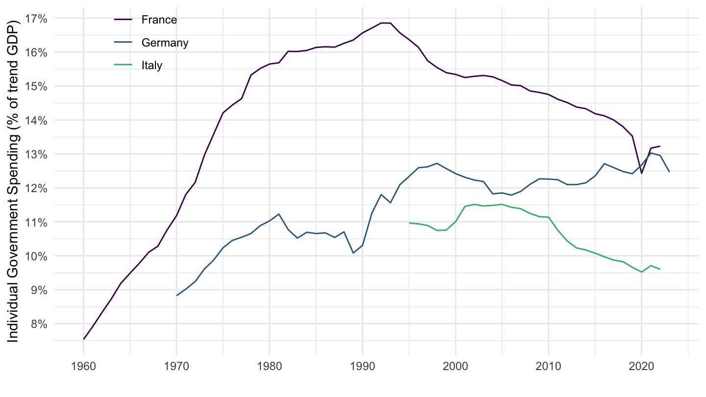
United Kingdom, Japan, United States
Code
SNA_TABLE1 %>%
  filter(MEASURE == "VXVOB",
         LOCATION %in% c("JPN", "GBR", "USA"),
         TRANSACT %in% c("B1_GE", "P31S13")) %>%
  year_to_date %>%
  left_join(SNA_TABLE1_var$LOCATION %>%
              setNames(c("LOCATION", "Location")), by = "LOCATION") %>%
  select(Location, date, TRANSACT, obsValue) %>%
  spread(TRANSACT, obsValue) %>%
  group_by(Location) %>%
  mutate(B1_GE_trend = log(B1_GE) %>% hpfilter(100000) %>% pluck("trend") %>% exp,
         P31S13_B1_GE_trend = P31S13 / B1_GE_trend,
         P31S13_B1_GE = P31S13 / B1_GE) %>%
  select(Location, date, P31S13_B1_GE_trend) %>%
  na.omit %>%
  ggplot() + geom_line(aes(x = date, y = P31S13_B1_GE_trend, color = Location)) +
  scale_color_manual(values = viridis(4)[1:3]) +
  theme_minimal() +
  scale_x_date(breaks = seq(1920, 2100, 10) %>% paste0("-01-01") %>% as.Date,
               labels = date_format("%Y")) +
  theme(legend.position = c(0.85, 0.9),
        legend.title = element_blank()) +
  scale_y_continuous(breaks = 0.01*seq(0, 100, 1),
                     labels = scales::percent_format(accuracy = 1)) +
  ylab("Individual Government Spending (% of trend GDP)") + xlab("")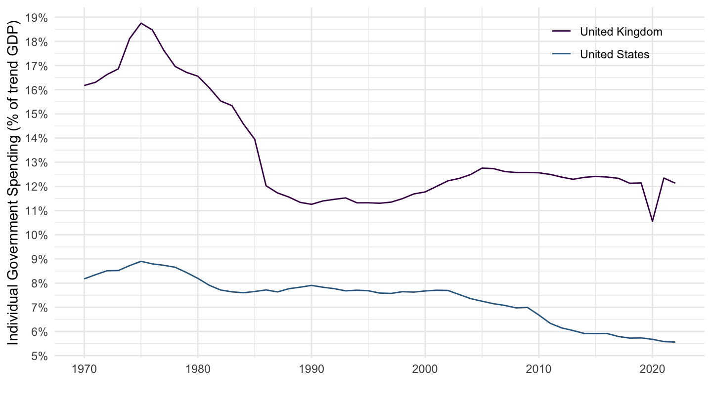
Switzerland, Germany, Netherlands
Code
SNA_TABLE1 %>%
  filter(MEASURE == "VXVOB",
         LOCATION %in% c("NLD", "CHE", "DEU"),
         TRANSACT %in% c("B1_GE", "P31S13")) %>%
  year_to_date %>%
  left_join(SNA_TABLE1_var$LOCATION %>%
              setNames(c("LOCATION", "Location")), by = "LOCATION") %>%
  select(Location, date, TRANSACT, obsValue) %>%
  spread(TRANSACT, obsValue) %>%
  group_by(Location) %>%
  mutate(B1_GE_trend = log(B1_GE) %>% hpfilter(100000) %>% pluck("trend") %>% exp,
         P31S13_B1_GE_trend = P31S13 / B1_GE_trend,
         P31S13_B1_GE = P31S13 / B1_GE) %>%
  select(Location, date, P31S13_B1_GE_trend) %>%
  na.omit %>%
  ggplot() + geom_line(aes(x = date, y = P31S13_B1_GE_trend, color = Location)) +
  scale_color_manual(values = viridis(4)[1:3]) +
  theme_minimal() +
  scale_x_date(breaks = seq(1920, 2100, 10) %>% paste0("-01-01") %>% as.Date,
               labels = date_format("%Y")) +
  theme(legend.position = c(0.15, 0.8),
        legend.title = element_blank()) +
  scale_y_continuous(breaks = 0.01*seq(0, 100, 1),
                     labels = scales::percent_format(accuracy = 1)) +
  ylab("Individual Government Spending (% of trend GDP)") + xlab("")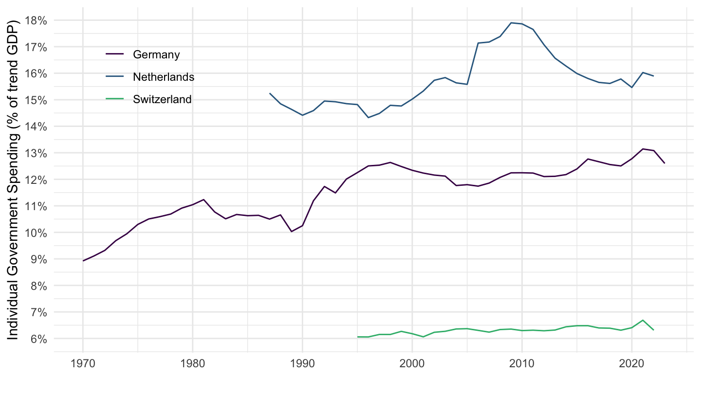
Collective Government Spending / trend GDP
France, Germany, Italy
Code
SNA_TABLE1 %>%
  filter(MEASURE == "VXVOB",
         LOCATION %in% c("FRA", "DEU", "ITA"),
         TRANSACT %in% c("B1_GE", "P32S13")) %>%
  year_to_date %>%
  left_join(SNA_TABLE1_var$LOCATION %>%
              setNames(c("LOCATION", "Location")), by = "LOCATION") %>%
  select(Location, date, TRANSACT, obsValue) %>%
  spread(TRANSACT, obsValue) %>%
  group_by(Location) %>%
  mutate(B1_GE_trend = log(B1_GE) %>% hpfilter(1000000) %>% pluck("trend") %>% exp,
         P32S13_B1_GE_trend = P32S13 / B1_GE_trend,
         P32S13_B1_GE = P32S13 / B1_GE) %>%
  select(Location, date, P32S13_B1_GE_trend) %>%
  na.omit %>%
  ggplot() + geom_line(aes(x = date, y = P32S13_B1_GE_trend, color = Location)) +
  scale_color_manual(values = viridis(4)[1:3]) +
  theme_minimal() +
  scale_x_date(breaks = seq(1920, 2100, 10) %>% paste0("-01-01") %>% as.Date,
               labels = date_format("%Y")) +
  theme(legend.position = c(0.15, 0.9),
        legend.title = element_blank()) +
  scale_y_continuous(breaks = 0.01*seq(0, 100, 1),
                     labels = scales::percent_format(accuracy = 1)) +
  ylab("Collective Government Spending (% of trend GDP)") + xlab("")
United Kingdom, Japan, United States
Code
SNA_TABLE1 %>%
  filter(MEASURE == "VXVOB",
         LOCATION %in% c("JPN", "GBR", "USA"),
         TRANSACT %in% c("B1_GE", "P32S13")) %>%
  year_to_date %>%
  left_join(SNA_TABLE1_var$LOCATION %>%
              setNames(c("LOCATION", "Location")), by = "LOCATION") %>%
  select(Location, date, TRANSACT, obsValue) %>%
  spread(TRANSACT, obsValue) %>%
  group_by(Location) %>%
  mutate(B1_GE_trend = log(B1_GE) %>% hpfilter(100000) %>% pluck("trend") %>% exp,
         P32S13_B1_GE_trend = P32S13 / B1_GE_trend,
         P32S13_B1_GE = P32S13 / B1_GE) %>%
  select(Location, date, P32S13_B1_GE_trend) %>%
  na.omit %>%
  ggplot() + geom_line(aes(x = date, y = P32S13_B1_GE_trend, color = Location)) +
  scale_color_manual(values = viridis(4)[1:3]) +
  theme_minimal() +
  scale_x_date(breaks = seq(1920, 2100, 10) %>% paste0("-01-01") %>% as.Date,
               labels = date_format("%Y")) +
  theme(legend.position = c(0.85, 0.9),
        legend.title = element_blank()) +
  scale_y_continuous(breaks = 0.01*seq(0, 100, 1),
                     labels = scales::percent_format(accuracy = 1)) +
  ylab("Collective Government Spending (% of trend GDP)") + xlab("")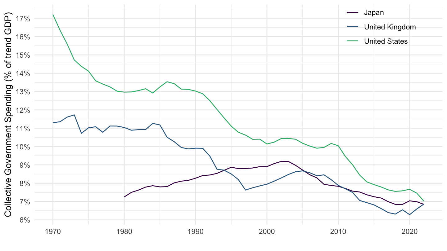
Switzerland, Germany, Netherlands
Code
SNA_TABLE1 %>%
  filter(MEASURE == "VXVOB",
         LOCATION %in% c("NLD", "CHE", "DEU"),
         TRANSACT %in% c("B1_GE", "P32S13")) %>%
  year_to_date %>%
  left_join(SNA_TABLE1_var$LOCATION %>%
              setNames(c("LOCATION", "Location")), by = "LOCATION") %>%
  select(Location, date, TRANSACT, obsValue) %>%
  spread(TRANSACT, obsValue) %>%
  group_by(Location) %>%
  mutate(B1_GE_trend = log(B1_GE) %>% hpfilter(100000) %>% pluck("trend") %>% exp,
         P32S13_B1_GE_trend = P32S13 / B1_GE_trend,
         P32S13_B1_GE = P32S13 / B1_GE) %>%
  select(Location, date, P32S13_B1_GE_trend) %>%
  na.omit %>%
  ggplot() + geom_line(aes(x = date, y = P32S13_B1_GE_trend, color = Location)) +
  scale_color_manual(values = viridis(4)[1:3]) +
  theme_minimal() +
  scale_x_date(breaks = seq(1920, 2100, 10) %>% paste0("-01-01") %>% as.Date,
               labels = date_format("%Y")) +
  theme(legend.position = c(0.15, 0.8),
        legend.title = element_blank()) +
  scale_y_continuous(breaks = 0.01*seq(0, 100, 1),
                     labels = scales::percent_format(accuracy = 1)) +
  ylab("Collective Government Spending (% of trend GDP)") + xlab("")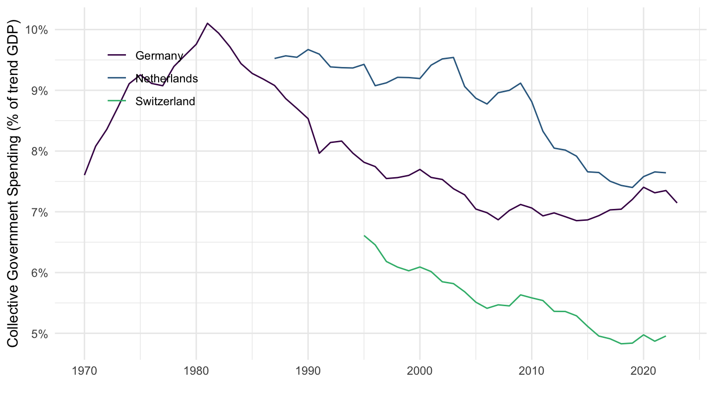
GDP / trend GDP
France, Germany, Italy
Code
SNA_TABLE1 %>%
  filter(MEASURE == "VXVOB",
         LOCATION %in% c("FRA", "DEU", "ITA"),
         TRANSACT %in% c("B1_GE", "B1_GE")) %>%
  year_to_date %>%
  left_join(SNA_TABLE1_var$LOCATION %>%
              setNames(c("LOCATION", "Location")), by = "LOCATION") %>%
  select(Location, date, TRANSACT, obsValue) %>%
  spread(TRANSACT, obsValue) %>%
  group_by(Location) %>%
  mutate(B1_GE_trend = log(B1_GE) %>% hpfilter(1000000) %>% pluck("trend") %>% exp,
         B1_GE_B1_GE_trend = B1_GE / B1_GE_trend,
         B1_GE_B1_GE = B1_GE / B1_GE) %>%
  select(Location, date, B1_GE_B1_GE_trend) %>%
  na.omit %>%
  ggplot() + geom_line(aes(x = date, y = B1_GE_B1_GE_trend, color = Location)) +
  scale_color_manual(values = viridis(4)[1:3]) +
  theme_minimal() +
  scale_x_date(breaks = seq(1920, 2100, 10) %>% paste0("-01-01") %>% as.Date,
               labels = date_format("%Y")) +
  theme(legend.position = c(0.85, 0.9),
        legend.title = element_blank()) +
  scale_y_continuous(breaks = 0.01*seq(0, 150, 5),
                     labels = scales::percent_format(accuracy = 1)) +
  ylab("GDP (% of trend GDP)") + xlab("")
United Kingdom, Japan, United States
Code
SNA_TABLE1 %>%
  filter(MEASURE == "VXVOB",
         LOCATION %in% c("JPN", "GBR", "USA"),
         TRANSACT %in% c("B1_GE", "B1_GE")) %>%
  year_to_date %>%
  left_join(SNA_TABLE1_var$LOCATION %>%
              setNames(c("LOCATION", "Location")), by = "LOCATION") %>%
  select(Location, date, TRANSACT, obsValue) %>%
  spread(TRANSACT, obsValue) %>%
  group_by(Location) %>%
  mutate(B1_GE_trend = log(B1_GE) %>% hpfilter(100000) %>% pluck("trend") %>% exp,
         B1_GE_B1_GE_trend = B1_GE / B1_GE_trend,
         B1_GE_B1_GE = B1_GE / B1_GE) %>%
  select(Location, date, B1_GE_B1_GE_trend) %>%
  na.omit %>%
  ggplot() + geom_line(aes(x = date, y = B1_GE_B1_GE_trend, color = Location)) +
  scale_color_manual(values = viridis(4)[1:3]) +
  theme_minimal() +
  scale_x_date(breaks = seq(1920, 2100, 10) %>% paste0("-01-01") %>% as.Date,
               labels = date_format("%Y")) +
  theme(legend.position = c(0.85, 0.9),
        legend.title = element_blank()) +
  scale_y_continuous(breaks = 0.01*seq(0, 200, 10),
                     labels = scales::percent_format(accuracy = 1)) +
  ylab("GDP (% of trend GDP)") + xlab("")
Switzerland, Germany, Netherlands
Code
SNA_TABLE1 %>%
  filter(MEASURE == "VXVOB",
         LOCATION %in% c("NLD", "CHE", "DEU"),
         TRANSACT %in% c("B1_GE", "B1_GE")) %>%
  year_to_date %>%
  left_join(SNA_TABLE1_var$LOCATION %>%
              setNames(c("LOCATION", "Location")), by = "LOCATION") %>%
  select(Location, date, TRANSACT, obsValue) %>%
  spread(TRANSACT, obsValue) %>%
  group_by(Location) %>%
  mutate(B1_GE_trend = log(B1_GE) %>% hpfilter(100000) %>% pluck("trend") %>% exp,
         B1_GE_B1_GE_trend = B1_GE / B1_GE_trend,
         B1_GE_B1_GE = B1_GE / B1_GE) %>%
  select(Location, date, B1_GE_B1_GE_trend) %>%
  na.omit %>%
  ggplot() + geom_line(aes(x = date, y = B1_GE_B1_GE_trend, color = Location)) +
  scale_color_manual(values = viridis(4)[1:3]) +
  theme_minimal() +
  scale_x_date(breaks = seq(1920, 2100, 10) %>% paste0("-01-01") %>% as.Date,
               labels = date_format("%Y")) +
  theme(legend.position = c(0.15, 0.3),
        legend.title = element_blank()) +
  scale_y_continuous(breaks = 0.01*seq(0, 200, 5),
                     labels = scales::percent_format(accuracy = 1)) +
  ylab("GDP (% of trend GDP)") + xlab("")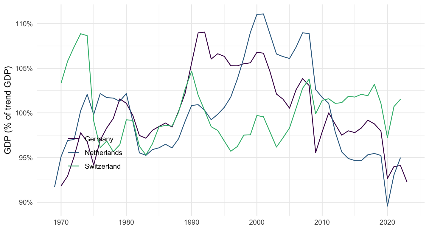
Japan
GDP: Nominal and Real
Code
SNA_TABLE1 %>%
  filter(LOCATION %in% c("JPN"),
         TRANSACT == "B1_GE",
         MEASURE %in% c("C", "V")) %>%
  mutate(date = paste0(obsTime, "-01-01") %>% as.Date) %>%
  left_join(SNA_TABLE1_var$LOCATION, by = "LOCATION") %>%
  left_join(SNA_TABLE1_var$MEASURE, by = "MEASURE") %>%
  group_by(LOCATION) %>%
  arrange(date) %>%
  select(date, obsValue, Measure) %>%
  ggplot(.) +
  geom_line(aes(x = date, y = obsValue / 10^6, linetype = Measure, color = Measure)) +
  theme_minimal() + xlab("") + ylab("") +
  scale_color_manual(values = viridis(4)[1:3]) +
  geom_rect(data = nber_recessions,
            aes(xmin = Peak, xmax = Trough, ymin = -Inf, ymax = +Inf),
            fill = 'grey', alpha = 0.5) +
  scale_x_date(breaks = seq(1960, 2100, 5) %>% paste0("-01-01") %>% as.Date,
               labels = date_format("%Y"),
               limits = c(1970, 2019) %>% paste0("-01-01") %>% as.Date) +
  scale_y_continuous(breaks = seq(0, 600, 50),
                     labels = dollar_format(suffix = " Tn", prefix = "¥", accuracy = 1)) +
  theme(legend.position = c(0.6, 0.20),
        legend.title = element_blank())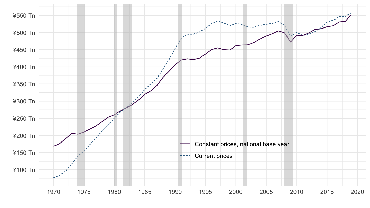
X and M
Code
SNA_TABLE1 %>%
  year_to_date %>%
  filter(TRANSACT %in% c("P6", "P7", "B1_GE"),
         MEASURE == "V",
         LOCATION == "JPN",
         date >= as.Date("1980-01-01"),
         date <= as.Date("1995-01-01")) %>%
  select(date, TRANSACT, obsValue) %>%
  spread(TRANSACT, obsValue) %>%
  mutate(`Real Exports (% of Real GDP)` = P6 / B1_GE,
         `Real Imports (% of Real GDP)` = P7 / B1_GE) %>%
  na.omit %>%
  select(-P6, -P7, -B1_GE) %>%
  gather(variable, value, - date) %>%
  ggplot() + geom_line(aes(x = date, y = value, color = variable)) +
  scale_color_manual(values = viridis(4)[1:3]) +
  theme_minimal() +
  scale_x_date(breaks = seq(1920, 2100, 1) %>% paste0("-01-01") %>% as.Date,
               labels = date_format("%Y")) +
  theme(legend.position = c(0.15, 0.9),
        legend.title = element_blank()) +
  scale_y_continuous(breaks = 0.01*seq(0, 60, 1),
                     labels = scales::percent_format(accuracy = 1)) +
  geom_vline(xintercept = as.Date("1985-09-22"), linetype = "dashed", color = viridis(4)[3]) +
  ylab("% of GDP (Japan)") + xlab("")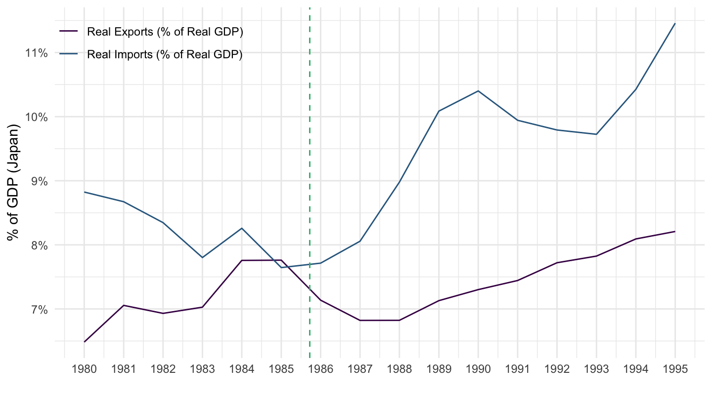
Nominal X and M
Code
SNA_TABLE1 %>%
  year_to_date %>%
  filter(TRANSACT %in% c("P6", "P7", "B1_GE"),
         MEASURE == "C",
         LOCATION == "JPN",
         date >= as.Date("1980-01-01"),
         date <= as.Date("1995-01-01")) %>%
  select(date, TRANSACT, obsValue) %>%
  spread(TRANSACT, obsValue) %>%
  mutate(`Exports (% of GDP)` = P6 / B1_GE,
         `Imports (% of GDP)` = P7 / B1_GE) %>%
  na.omit %>%
  select(-P6, -P7, -B1_GE) %>%
  gather(variable, value, - date) %>%
  ggplot() + geom_line(aes(x = date, y = value, color = variable)) +
  scale_color_manual(values = viridis(4)[1:3]) +
  theme_minimal() +
  scale_x_date(breaks = seq(1920, 2100, 1) %>% paste0("-01-01") %>% as.Date,
               labels = date_format("%Y")) +
  theme(legend.position = c(0.75, 0.9),
        legend.title = element_blank()) +
  scale_y_continuous(breaks = 0.01*seq(0, 60, 1),
                     labels = scales::percent_format(accuracy = 1)) +
  geom_vline(xintercept = as.Date("1985-09-22"), linetype = "dashed", color = viridis(4)[3]) +
  ylab("% of GDP (Japan)") + xlab("")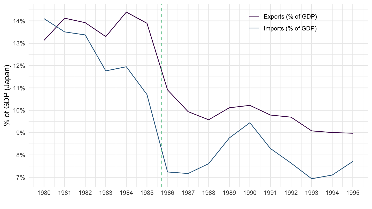
Around 1990
Code
SNA_TABLE1 %>%
  filter(LOCATION %in% c("JPN"),
         TRANSACT %in% c("B1_GE", "P31S14", "P5"),
         MEASURE == "C") %>%
  year_to_date %>%
  left_join(SNA_TABLE1_var$TRANSACT, by = "TRANSACT") %>%
  group_by(LOCATION) %>%
  arrange(date) %>%
  select(date, obsValue, Transact) %>%
  ggplot(.) +
  geom_line(aes(x = date, y = obsValue / 10^6, linetype = Transact, color = Transact)) +
  theme_minimal() + xlab("") + ylab("") +
  scale_color_manual(values = viridis(4)[1:3]) +
  geom_rect(data = nber_recessions,
            aes(xmin = Peak, xmax = Trough, ymin = -Inf, ymax = +Inf),
            fill = 'grey', alpha = 0.5) +
  scale_x_date(breaks = seq(1960, 2100, 5) %>% paste0("-01-01") %>% as.Date,
               labels = date_format("%Y"),
               limits = c(1970, 2019) %>% paste0("-01-01") %>% as.Date) +
  scale_y_continuous(breaks = seq(0, 1000, 100),
                     labels = dollar_format(suffix = " Tn", prefix = "¥", accuracy = 1),
                     limits = c(0, 800)) +
  theme(legend.position = c(0.4, 0.9),
        legend.title = element_blank())
Investment
Investment Rate - Compare
Code
SNA_TABLE1 %>%
  filter(obsTime == "2018",
         MEASURE == "C",
         grepl("^P51", TRANSACT) | TRANSACT == "B1_GE") %>%
  left_join(SNA_TABLE1_var$TRANSACT, by = "TRANSACT") %>%
  left_join(SNA_TABLE1_var$LOCATION, by = "LOCATION") %>%
  group_by(Location) %>%
  mutate(obsValue = 100*obsValue / obsValue[TRANSACT == "B1_GE"]) %>%
  filter(TRANSACT != "B1_GE") %>%
  select(Location, Transact, obsValue) %>%
  na.omit %>%
  spread(Transact, obsValue) %>%
  arrange(-`Gross fixed capital formation`) %>%
  mutate_at(vars(-1), funs(ifelse(is.na(.), NA, paste0(round(., 1), "%")))) %>%
  select(1, 4, 2, 3, 5, 6, 7) %>%
{if (is_html_output()) print_table(.) else .}| Location | Computer software and databases | Computer Hardware | Computer software | Cultivated biological resources | Dwellings | Entertainment, literary and artistic originals |
|---|---|---|---|---|---|---|
| China (People's Republic of) | NA | NA | NA | NA | NA | NA |
| Zambia | NA | NA | NA | NA | NA | NA |
| Indonesia | NA | NA | NA | 1.8% | 24% | NA |
| Korea | NA | NA | NA | NA | 5.8% | NA |
| Turkey | NA | NA | NA | NA | NA | NA |
| Morocco | NA | NA | NA | NA | NA | NA |
| Ireland | NA | NA | NA | 0% | 2.3% | NA |
| Czech Republic | NA | NA | NA | 0.1% | 4.3% | NA |
| Switzerland | NA | NA | NA | 0% | 4.8% | NA |
| Sweden | NA | NA | NA | 0% | 5.2% | NA |
| Hungary | NA | NA | NA | 0.1% | 3% | NA |
| Estonia | NA | NA | NA | 0.1% | 4.5% | NA |
| Finland | NA | NA | NA | 0% | 7.3% | NA |
| Japan | 1.9% | NA | 1.9% | 0% | 3.1% | NA |
| Austria | NA | NA | NA | 0% | 4.5% | NA |
| Norway | NA | NA | NA | 0% | 5.4% | NA |
| Albania | NA | NA | NA | 0.2% | 10.8% | NA |
| Belgium | NA | NA | NA | 0% | 5.9% | NA |
| New Zealand | NA | 0.8% | NA | NA | 7.4% | NA |
| Australia | 1.1% | 0.3% | NA | 0.2% | 5.7% | 0.1% |
| Singapore | NA | NA | NA | NA | 3.6% | NA |
| France | NA | NA | NA | 0% | 6.4% | NA |
| Canada | NA | NA | NA | NA | 7.6% | NA |
| Latvia | 0.7% | 0.9% | NA | 0.1% | 2.5% | 0.2% |
| Mexico | 0% | 0.4% | 0% | 0% | 6% | 0% |
| Denmark | NA | NA | NA | 0% | 4.8% | NA |
| Hong Kong, China | NA | NA | NA | NA | NA | NA |
| Iceland | NA | NA | NA | 0% | 4.3% | NA |
| Israel | NA | NA | NA | 0% | 6.6% | NA |
| Colombia | 0.3% | 0.4% | NA | 0.5% | 5% | 0% |
| Chile | NA | NA | NA | NA | NA | NA |
| Germany | NA | NA | NA | 0% | 6.3% | NA |
| Malta | NA | NA | NA | 0% | 5.1% | NA |
| Romania | NA | NA | NA | 0% | 2% | NA |
| Euro area (19 countries) | NA | NA | NA | 0.1% | 5.4% | NA |
| Saudi Arabia | NA | NA | NA | NA | NA | NA |
| Slovak Republic | NA | NA | NA | 0.7% | 3.4% | NA |
| Lithuania | NA | NA | NA | 0.2% | 2.7% | NA |
| Madagascar | NA | NA | NA | NA | NA | NA |
| United States | 2.1% | 0.6% | 2.1% | NA | 3.8% | 0.4% |
| Netherlands | NA | NA | NA | 0% | 4.9% | NA |
| Croatia | NA | NA | NA | NA | NA | NA |
| Serbia | NA | NA | NA | 0.3% | 1.4% | NA |
| North Macedonia | NA | NA | NA | 0.1% | 3.9% | NA |
| Russia | NA | NA | NA | NA | NA | NA |
| Spain | NA | NA | NA | 0.2% | 5.4% | NA |
| Slovenia | NA | NA | NA | 0.1% | 2.1% | NA |
| Cyprus | NA | NA | NA | 0% | 6.5% | NA |
| Bulgaria | NA | NA | NA | 0.2% | 2.7% | NA |
| Poland | NA | NA | NA | 0% | 1.9% | NA |
| South Africa | NA | NA | NA | 0.2% | 1.8% | NA |
| Italy | NA | NA | NA | 0% | 4.1% | NA |
| United Kingdom | NA | NA | NA | 0.1% | 4% | NA |
| Costa Rica | NA | NA | NA | 0.2% | 3.5% | NA |
| Portugal | NA | NA | NA | 0.2% | 3.1% | NA |
| Luxembourg | NA | NA | NA | 0% | 3.8% | NA |
| Argentina | NA | NA | NA | NA | NA | NA |
| Greece | NA | NA | NA | 0% | 0.7% | NA |
P51 - Investment
Code
SNA_TABLE1 %>%
  filter(LOCATION %in% c("USA"),
         TRANSACT == "P51",
         MEASURE %in% c("C", "V")) %>%
  mutate(date = paste0(obsTime, "-01-01") %>% as.Date,
         obsValue = obsValue / 10^6) %>%
  left_join(SNA_TABLE1_var$LOCATION, by = "LOCATION") %>%
  left_join(SNA_TABLE1_var$MEASURE, by = "MEASURE") %>%
  group_by(LOCATION) %>%
  arrange(date) %>%
  select(date, obsValue, Measure) %>%
  ggplot(.) + geom_line(aes(x = date, y = obsValue, linetype = Measure, color = Measure)) +
  theme_minimal() + xlab("") + ylab("") +
  scale_color_manual(values = viridis(4)[1:3]) +
  geom_rect(data = nber_recessions,
            aes(xmin = Peak, xmax = Trough, ymin = -Inf, ymax = +Inf),
            fill = 'grey', alpha = 0.5) +
  scale_x_date(breaks = seq(1960, 2100, 5) %>% paste0("-01-01") %>% as.Date,
               labels = date_format("%Y"),
               limits = c(1970, 2019) %>% paste0("-01-01") %>% as.Date) +
  scale_y_continuous(breaks = seq(0, 10, 0.5),
                     labels = dollar_format(suffix = "Tn", prefix = "$", accuracy = 0.1)) +
  theme(legend.position = c(0.3, 0.90),
        legend.title = element_blank())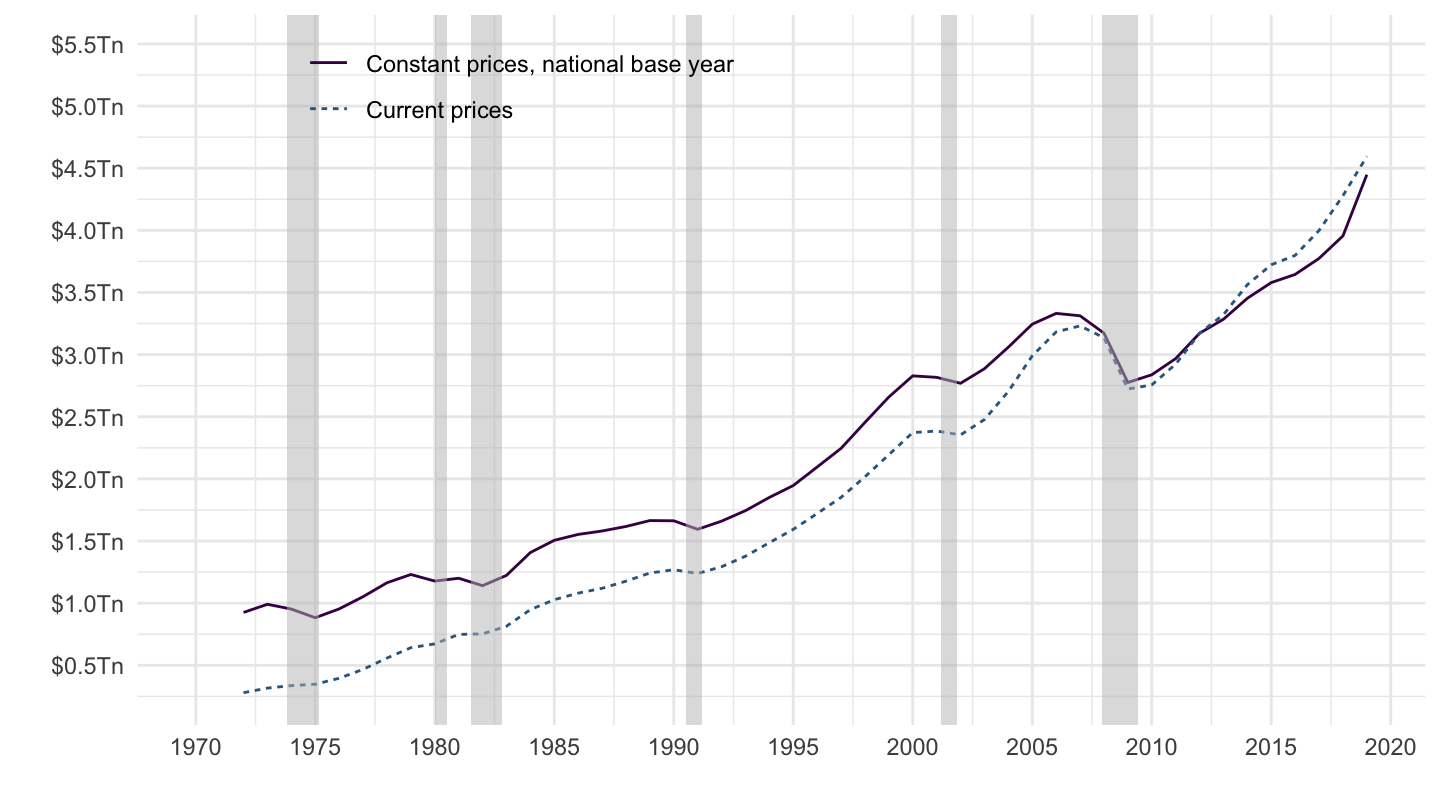
P51N1113 - Machinery and equipment and weapon system
Code
SNA_TABLE1 %>%
  filter(LOCATION %in% c("USA"),
         TRANSACT == "P51N1113",
         MEASURE %in% c("C", "V")) %>%
  mutate(date = paste0(obsTime, "-01-01") %>% as.Date,
         obsValue = obsValue / 10^6) %>%
  left_join(SNA_TABLE1_var$LOCATION, by = "LOCATION") %>%
  left_join(SNA_TABLE1_var$MEASURE, by = "MEASURE") %>%
  group_by(LOCATION) %>%
  arrange(date) %>%
  select(date, obsValue, Measure) %>%
  ggplot(.) + geom_line(aes(x = date, y = obsValue, linetype = Measure, color = Measure)) +
  theme_minimal() + xlab("") + ylab("") +
  scale_color_manual(values = viridis(4)[1:3]) +
  geom_rect(data = nber_recessions,
            aes(xmin = Peak, xmax = Trough, ymin = -Inf, ymax = +Inf),
            fill = 'grey', alpha = 0.5) +
  scale_x_date(breaks = seq(1960, 2100, 5) %>% paste0("-01-01") %>% as.Date,
               labels = date_format("%Y"),
               limits = c(1970, 2019) %>% paste0("-01-01") %>% as.Date) +
  scale_y_continuous(breaks = seq(0, 2, 0.2),
                     labels = dollar_format(suffix = "Tn", prefix = "$", accuracy = 0.1)) +
  theme(legend.position = c(0.3, 0.90),
        legend.title = element_blank())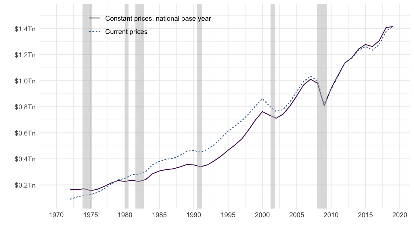
Net Exports
X - M, Total, Goods, Services
Code
SNA_TABLE1 %>%
  filter(obsTime == "2018",
         MEASURE == "C",
         TRANSACT %in% c("B1_GE", "P61", "P71", "P62", "P72", "P6", "P7")) %>%
  left_join(SNA_TABLE1_var$LOCATION, by = "LOCATION") %>%
  left_join(SNA_TABLE1_var$MEASURE, by = "MEASURE") %>%
  group_by(LOCATION, Location) %>%
  mutate(obsValue = 100*obsValue / obsValue[TRANSACT == "B1_GE"]) %>%
  filter(TRANSACT != "B1_GE") %>%
  select(LOCATION, Location, TRANSACT, obsValue) %>%
  na.omit %>%
  spread(TRANSACT, obsValue) %>%
  mutate_at(vars(-1, -2), funs(ifelse(is.na(.), NA, paste0(round(., 1), "%")))) %>%
  mutate(Flag = gsub(" ", "-", str_to_lower(gsub(" ", "-", Location))),
         Flag = paste0('<img src="../../icon/flag/vsmall/', Flag, '.png" alt="Flag">')) %>%
  select(Flag, everything()) %>%
  {if (is_html_output()) datatable(., filter = 'top', rownames = F, escape = F) else .}
Code
include_graphics3b("bib/oecd/SNA_TABLE1_X_M.png")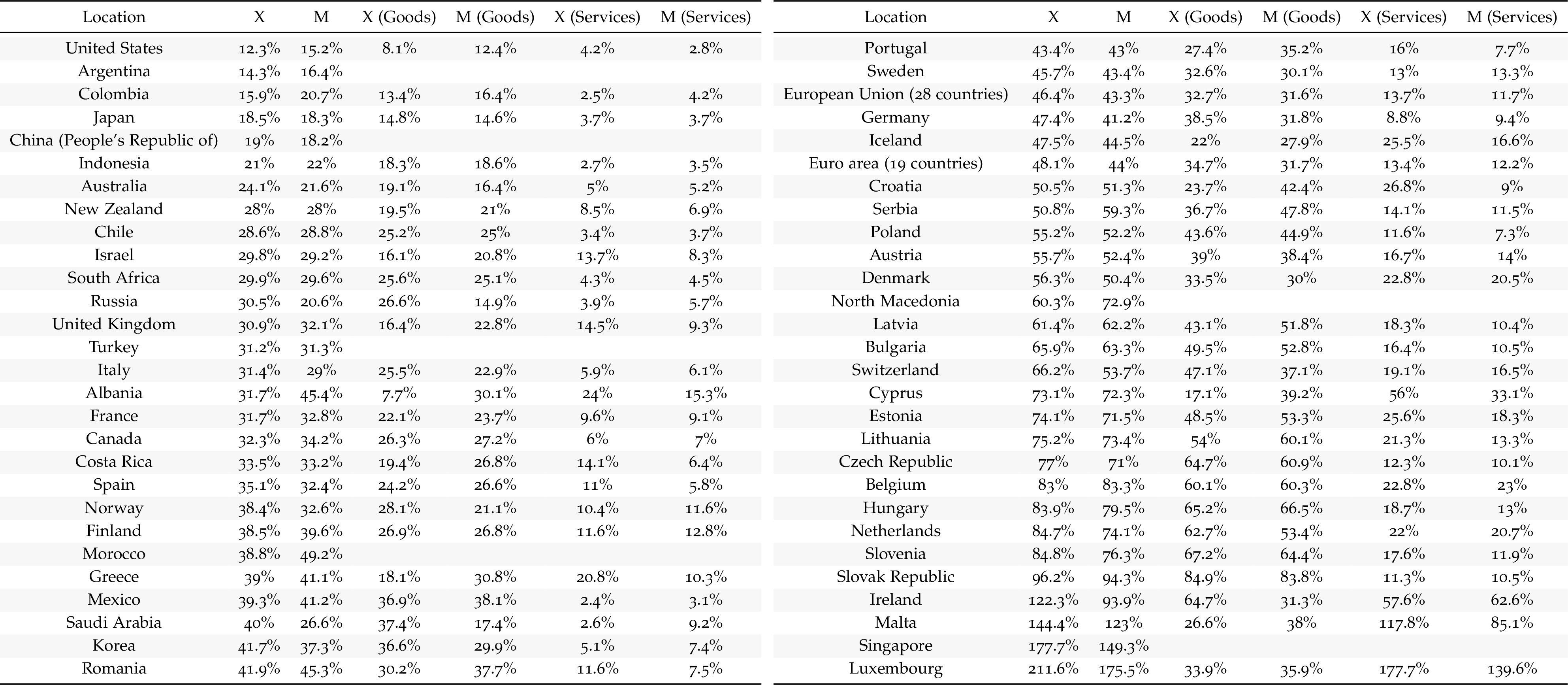
France, Germany, United Kingdom
NX
Code
SNA_TABLE1 %>%
  filter(LOCATION %in% c("DEU", "FRA", "GBR"),
         MEASURE == "C",
         TRANSACT %in% c("B1_GE", "P61", "P71", "P62", "P72", "P6", "P7")) %>%
  year_to_date %>%
  left_join(SNA_TABLE1_var$LOCATION, by = "LOCATION") %>%
  left_join(SNA_TABLE1_var$MEASURE, by = "MEASURE") %>%
  group_by(Location, date) %>%
  mutate(obsValue = 100*obsValue / obsValue[TRANSACT == "B1_GE"]) %>%
  filter(TRANSACT != "B1_GE") %>%
  select(Location, TRANSACT, obsValue) %>%
  na.omit %>%
  spread(TRANSACT, obsValue) %>%
  mutate(NX = P6 - P7,
         `Goods NX` = P61 - P71,
         `Services NX` = P62 - P72) %>%
  select(Location, NX, `Goods NX`, `Services NX`) %>%
  arrange(-`Goods NX`) %>%
  na.omit %>%
  mutate(obsValue = `NX`/100) %>%
  left_join(colors, by = c("Location" = "country")) %>%
  ggplot() + geom_line(aes(x = date, y = obsValue, color = color)) +
  ylab("Manufacturing Value Added (% of GDP)") + xlab("") +
  scale_color_identity() + theme_minimal() + add_3flags +
  scale_x_date(breaks = seq(1920, 2100, 5) %>% paste0("-01-01") %>% as.Date,
               labels = date_format("%Y")) +
  scale_y_continuous(breaks = 0.01*seq(-60, 60, 1),
                     labels = scales::percent_format(accuracy = 1))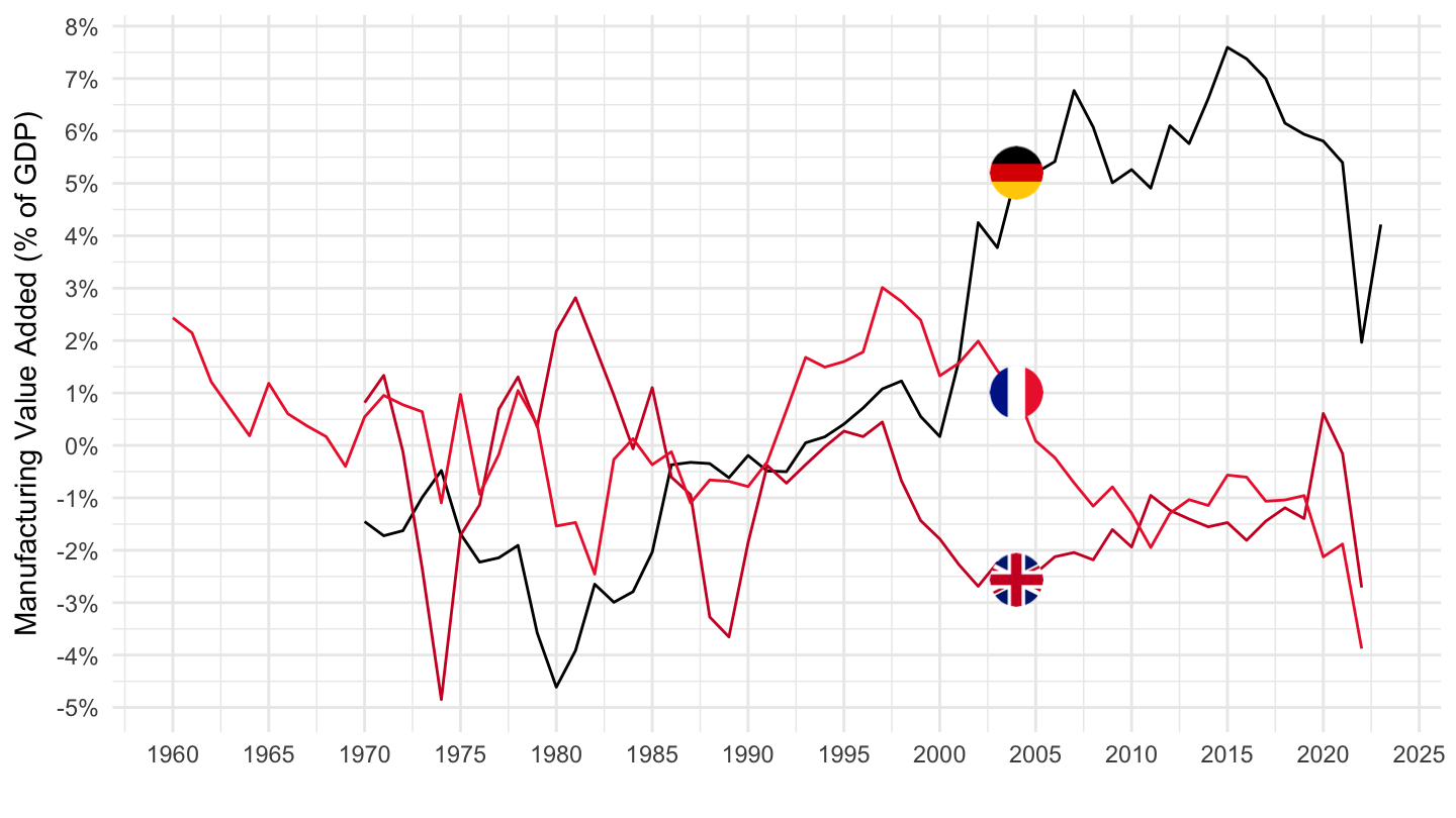
NX
Code
SNA_TABLE1 %>%
  filter(LOCATION %in% c("DEU", "FRA"),
         MEASURE == "C",
         TRANSACT %in% c("B1_GE", "P61", "P71", "P62", "P72", "P6", "P7")) %>%
  year_to_date %>%
  left_join(SNA_TABLE1_var$LOCATION, by = "LOCATION") %>%
  group_by(Location, date) %>%
  mutate(obsValue = 100*obsValue / obsValue[TRANSACT == "B1_GE"]) %>%
  filter(TRANSACT != "B1_GE",
         date >= as.Date("1990-01-01")) %>%
  select(Location, TRANSACT, obsValue) %>%
  na.omit %>%
  spread(TRANSACT, obsValue) %>%
  left_join(tibble(Location = c("France", "Germany"),
                   LocationF = c("France", "Allemagne")), by = "Location") %>%
  mutate(NX = P6 - P7,
         `Goods NX` = P61 - P71,
         `Services NX` = P62 - P72) %>%
  na.omit %>%
  mutate(obsValue = `NX`/100) %>%
  left_join(colors, by = c("Location" = "country")) %>%
  ggplot() + geom_line(aes(x = date, y = obsValue, color = color)) +
  ylab("Manufacturing Value Added (% of GDP)") + xlab("") +
  scale_color_identity() + theme_minimal() + add_2flags +
  scale_x_date(breaks = seq(1920, 2100, 5) %>% paste0("-01-01") %>% as.Date,
               labels = date_format("%Y")) +
  scale_y_continuous(breaks = 0.01*seq(-60, 60, 1),
                     labels = scales::percent_format(accuracy = 1))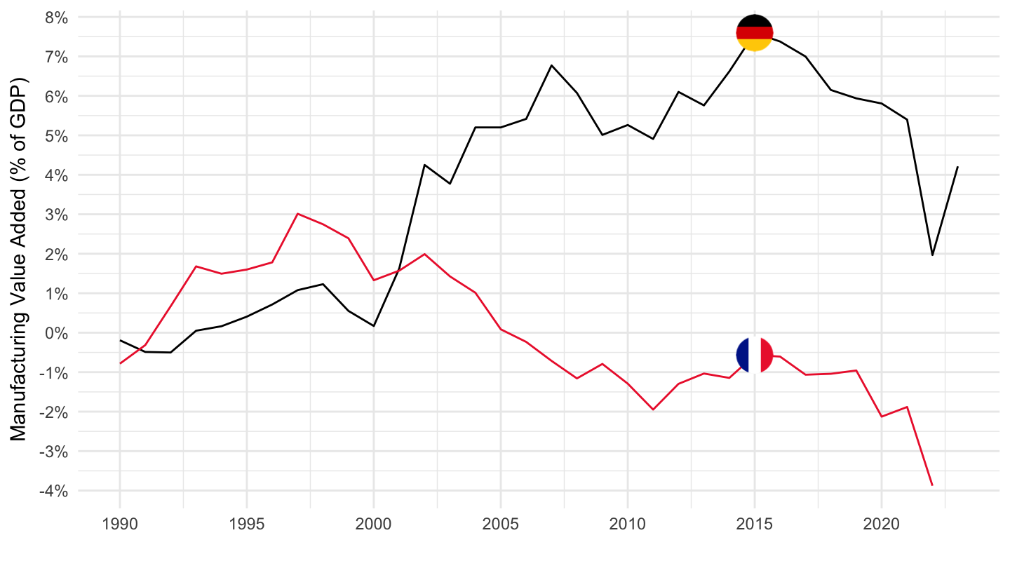
Goods NX
Code
SNA_TABLE1 %>%
  filter(LOCATION %in% c("DEU", "FRA", "GBR"),
         MEASURE == "C",
         TRANSACT %in% c("B1_GE", "P61", "P71", "P62", "P72", "P6", "P7")) %>%
  year_to_date %>%
  left_join(SNA_TABLE1_var$LOCATION, by = "LOCATION") %>%
  group_by(Location, date) %>%
  mutate(obsValue = 100*obsValue / obsValue[TRANSACT == "B1_GE"]) %>%
  filter(TRANSACT != "B1_GE") %>%
  select(Location, TRANSACT, obsValue) %>%
  na.omit %>%
  spread(TRANSACT, obsValue) %>%
  mutate(NX = P6 - P7,
         `Goods NX` = P61 - P71,
         `Services NX` = P62 - P72) %>%
  select(Location, NX, `Goods NX`, `Services NX`) %>%
  arrange(-`Goods NX`) %>%
  na.omit %>%
  mutate(obsValue = `NX`/100) %>%
  left_join(colors, by = c("Location" = "country")) %>%
  ggplot() + geom_line(aes(x = date, y = obsValue, color = color)) +
  ylab("Manufacturing Value Added (% of GDP)") + xlab("") +
  scale_color_identity() + theme_minimal() + add_3flags +
  scale_x_date(breaks = seq(1920, 2100, 5) %>% paste0("-01-01") %>% as.Date,
               labels = date_format("%Y")) +
  scale_y_continuous(breaks = 0.01*seq(-60, 60, 1),
                     labels = scales::percent_format(accuracy = 1))
Code
SNA_TABLE1 %>%
  filter(LOCATION %in% c("DEU", "FRA"),
         MEASURE == "C",
         TRANSACT %in% c("B1_GE", "P61", "P71", "P62", "P72", "P6", "P7")) %>%
  year_to_date %>%
  left_join(SNA_TABLE1_var$LOCATION, by = "LOCATION") %>%
  group_by(Location, date) %>%
  mutate(obsValue = 100*obsValue / obsValue[TRANSACT == "B1_GE"]) %>%
  filter(TRANSACT != "B1_GE",
         date >= as.Date("1990-01-01")) %>%
  select(Location, TRANSACT, obsValue) %>%
  na.omit %>%
  spread(TRANSACT, obsValue) %>%
  left_join(tibble(Location = c("France", "Germany"),
                   LocationF = c("France", "Allemagne")), by = "Location") %>%
  mutate(NX = P6 - P7,
         `Goods NX` = P61 - P71,
         `Services NX` = P62 - P72) %>%
  na.omit %>%
  mutate(obsValue = `Goods NX`/100) %>%
  left_join(colors, by = c("Location" = "country")) %>%
  ggplot() + geom_line(aes(x = date, y = obsValue, color = color)) +
  ylab("Goods Net Exports (% of GDP)") + xlab("") +
  scale_color_identity() + theme_minimal() + add_2flags +
  scale_x_date(breaks = seq(1920, 2100, 5) %>% paste0("-01-01") %>% as.Date,
               labels = date_format("%Y")) +
  scale_y_continuous(breaks = 0.01*seq(-60, 60, 1),
                     labels = scales::percent_format(accuracy = 1))
Services NX
Code
SNA_TABLE1 %>%
  filter(LOCATION %in% c("DEU", "FRA", "GBR"),
         MEASURE == "C",
         TRANSACT %in% c("B1_GE", "P61", "P71", "P62", "P72", "P6", "P7")) %>%
  year_to_date %>%
  left_join(SNA_TABLE1_var$LOCATION, by = "LOCATION") %>%
  group_by(Location, date) %>%
  mutate(obsValue = 100*obsValue / obsValue[TRANSACT == "B1_GE"]) %>%
  filter(TRANSACT != "B1_GE") %>%
  select(Location, TRANSACT, obsValue) %>%
  na.omit %>%
  spread(TRANSACT, obsValue) %>%
  mutate(NX = P6 - P7,
         `Goods NX` = P61 - P71,
         `Services NX` = P62 - P72) %>%
  select(Location, NX, `Goods NX`, `Services NX`) %>%
  arrange(-`Goods NX`) %>%
  na.omit %>%
  mutate(obsValue = `Services NX`/100) %>%
  left_join(colors, by = c("Location" = "country")) %>%
  ggplot() + geom_line(aes(x = date, y = obsValue, color = color)) +
  ylab("Services Net Exports (% of GDP)") + xlab("") +
  scale_color_identity() + theme_minimal() + add_3flags +
  scale_x_date(breaks = seq(1920, 2100, 5) %>% paste0("-01-01") %>% as.Date,
               labels = date_format("%Y")) +
  scale_y_continuous(breaks = 0.01*seq(-60, 60, 1),
                     labels = scales::percent_format(accuracy = 1))
Code
SNA_TABLE1 %>%
  filter(LOCATION %in% c("DEU", "FRA"),
         MEASURE == "C",
         TRANSACT %in% c("B1_GE", "P61", "P71", "P62", "P72", "P6", "P7")) %>%
  year_to_date %>%
  left_join(SNA_TABLE1_var$LOCATION, by = "LOCATION") %>%
  group_by(Location, date) %>%
  mutate(obsValue = 100*obsValue / obsValue[TRANSACT == "B1_GE"]) %>%
  filter(TRANSACT != "B1_GE",
         date >= as.Date("1990-01-01")) %>%
  select(Location, TRANSACT, obsValue) %>%
  na.omit %>%
  spread(TRANSACT, obsValue) %>%
  left_join(tibble(Location = c("France", "Germany"),
                   LocationF = c("France", "Allemagne")), by = "Location") %>%
  mutate(NX = P6 - P7,
         `Goods NX` = P61 - P71,
         `Services NX` = P62 - P72) %>%
  na.omit %>%
  ggplot() + geom_line(aes(x = date, y = `Services NX`/100, color = Location)) +
  scale_color_manual(values = viridis(4)[1:3]) +
  theme_minimal() +
  geom_hline(yintercept = 0, linetype = "dashed",  color = viridis(4)[3]) +
  scale_x_date(breaks = seq(1920, 2100, 2) %>% paste0("-01-01") %>% as.Date,
               labels = date_format("%Y")) +
  theme(legend.position = c(0.15, 0.5),
        legend.title = element_blank()) +
  scale_y_continuous(breaks = 0.01*seq(-10, 100, 1),
                     labels = scales::percent_format(accuracy = 1)) +
  ylab("Exportations Nettes de Services (% of PIB)") + xlab("")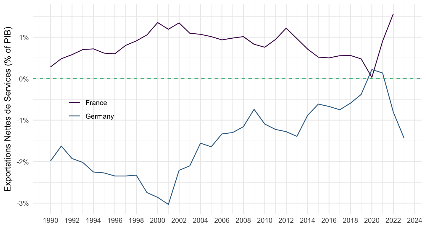
Deindustrialization and Financial Services
United Kingdom
Code
SNA_TABLE1 %>%
  filter(LOCATION %in% c("GBR"),
         MEASURE == "C",
         TRANSACT %in% c("B1_GE", "P61", "P71", "P62", "P72", "P6", "P7")) %>%
  year_to_date %>%
  select(date, TRANSACT, obsValue) %>%
  spread(TRANSACT, obsValue) %>%
  transmute(date,
            NX = P6/B1_GE - P7/B1_GE,
            NX1 = P61/B1_GE - P71/B1_GE,
            NX2 = P62/B1_GE - P72/B1_GE) %>%
  gather(variable, value, -date) %>%
  mutate(variable = factor(variable,
                           levels=c("NX2", "NX", "NX1"),
                           labels=c("Services", "Biens et Services", "Biens"))) %>%
  na.omit %>%
  ggplot() + geom_line() + theme_minimal() +
  aes(x = date, y = value, color = variable) +
  scale_color_manual(values = viridis(4)[1:3]) +
  scale_x_date(breaks = seq(1920, 2100, 10) %>% paste0("-01-01") %>% as.Date,
               labels = date_format("%Y")) +
  theme(legend.position = c(0.2, 0.9),
        legend.title = element_blank()) +
  scale_y_continuous(breaks = 0.01*seq(-10, 100, 1),
                     labels = scales::percent_format(accuracy = 1),
                     limits = c(-0.07, 0.06)) +
  labs(x = "",
       y = "Balance Commerciale, Royaume-Uni (% du PIB)")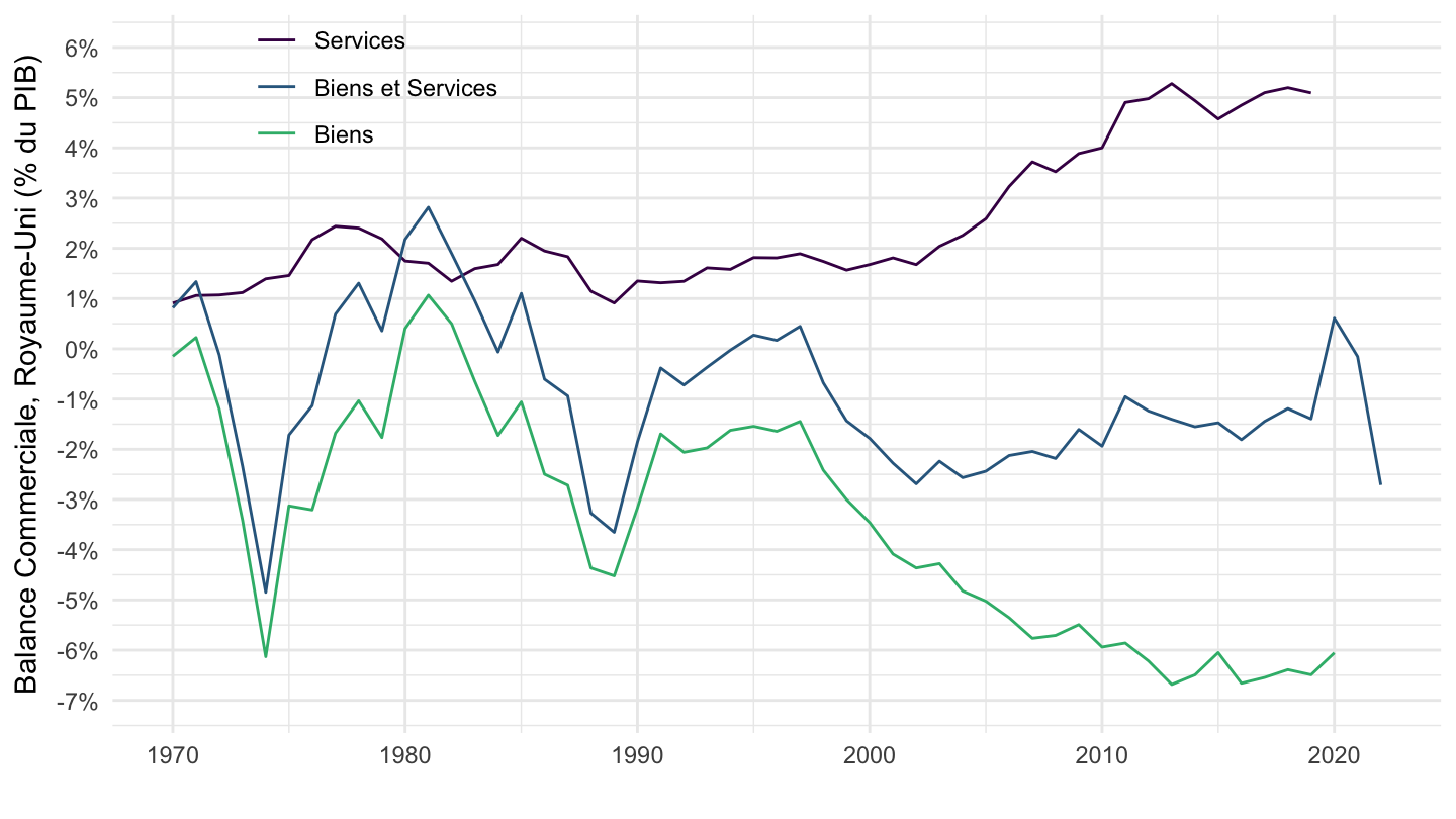
France
Code
SNA_TABLE1 %>%
  filter(LOCATION %in% c("FRA"),
         MEASURE == "C",
         TRANSACT %in% c("B1_GE", "P61", "P71", "P62", "P72", "P6", "P7")) %>%
  year_to_date %>%
  select(date, TRANSACT, obsValue) %>%
  spread(TRANSACT, obsValue) %>%
  transmute(date,
            NX = P6/B1_GE - P7/B1_GE,
            NX1 = P61/B1_GE - P71/B1_GE,
            NX2 = P62/B1_GE - P72/B1_GE) %>%
  gather(variable, value, -date) %>%
  mutate(variable = factor(variable,
                           levels=c("NX2", "NX", "NX1"),
                           labels=c("Services", "Biens et Services", "Biens"))) %>%
  na.omit %>%
  ggplot() + geom_line() + theme_minimal() +
  aes(x = date, y = value, color = variable) +
  scale_color_manual(values = viridis(4)[1:3]) +
  scale_x_date(breaks = seq(1920, 2100, 10) %>% paste0("-01-01") %>% as.Date,
               labels = date_format("%Y")) +
  theme(legend.position = c(0.2, 0.9),
        legend.title = element_blank()) +
  scale_y_continuous(breaks = 0.01*seq(-10, 100, 1),
                     labels = scales::percent_format(accuracy = 1),
                     limits = c(-0.07, 0.06)) +
  labs(x = "",
       y = "Balance Commerciale, France (% du PIB)")
Imports, Exports
France
Code
SNA_TABLE1 %>%
  filter(LOCATION == "FRA",
         MEASURE == "C",
         TRANSACT %in% c("B1_GE", "P61", "P71", "P62", "P72")) %>%
  left_join(SNA_TABLE1_var$TRANSACT, by = "TRANSACT") %>%
  year_to_date %>%
  group_by(date) %>%
  mutate(obsValue = obsValue / obsValue[TRANSACT == "B1_GE"]) %>%
  mutate(TRANSACT = factor(TRANSACT,
                           levels=c("P71", "P61", "P72", "P62"),
                           labels=c("Importations - Biens", "Exportations - Biens",
                                    "Importations - Services", "Exportations - Services"))) %>%
  filter(TRANSACT != "B1_GE") %>%
  ggplot() + theme_minimal() + ylab("% du PIB") + xlab("") +
  geom_line(aes(x = date, y = obsValue, color = TRANSACT, linetype = TRANSACT)) +
  scale_color_manual(values = c(viridis(3)[1], viridis(3)[1], viridis(3)[2], viridis(3)[2])) +
  scale_linetype_manual(values = c("solid",  "dashed", "solid", "dashed")) +
  scale_x_date(breaks = seq(1920, 2100, 5) %>% paste0("-01-01") %>% as.Date,
               labels = date_format("%Y")) +
  theme(legend.position = c(0.15, 0.85),
        legend.title = element_blank()) +
  scale_y_continuous(breaks = 0.01*seq(-60, 60, 2),
                     labels = scales::percent_format(accuracy = 1))
United States
Code
SNA_TABLE1 %>%
  filter(LOCATION == "USA",
         MEASURE == "C",
         TRANSACT %in% c("B1_GE", "P61", "P71", "P62", "P72")) %>%
  left_join(SNA_TABLE1_var$TRANSACT, by = "TRANSACT") %>%
  year_to_date %>%
  group_by(date) %>%
  mutate(obsValue = obsValue / obsValue[TRANSACT == "B1_GE"]) %>%
  mutate(TRANSACT = factor(TRANSACT,
                           levels=c("P71", "P61", "P72", "P62"),
                           labels=c("Importations - Biens", "Exportations - Biens",
                                    "Importations - Services", "Exportations - Services"))) %>%
  filter(TRANSACT != "B1_GE") %>%
  ggplot() + theme_minimal() + ylab("% of GDP") + xlab("") +
  geom_line(aes(x = date, y = obsValue, color = TRANSACT, linetype = TRANSACT)) +
  scale_color_manual(values = c(viridis(3)[1], viridis(3)[1], viridis(3)[2], viridis(3)[2])) +
  scale_linetype_manual(values = c("solid",  "dashed", "solid", "dashed")) +
  scale_x_date(breaks = seq(1920, 2100, 5) %>% paste0("-01-01") %>% as.Date,
               labels = date_format("%Y")) +
  theme(legend.position = c(0.15, 0.85),
        legend.title = element_blank()) +
  scale_y_continuous(breaks = 0.01*seq(-60, 60, 2),
                     labels = scales::percent_format(accuracy = 1))
China
Code
SNA_TABLE1 %>%
  filter(LOCATION == "CHN",
         MEASURE == "C",
         TRANSACT %in% c("B1_GE", "P61", "P71", "P62", "P72")) %>%
  left_join(SNA_TABLE1_var$TRANSACT, by = "TRANSACT") %>%
  year_to_date %>%
  group_by(date) %>%
  mutate(obsValue = obsValue / obsValue[TRANSACT == "B1_GE"]) %>%
  mutate(TRANSACT = factor(TRANSACT,
                           levels=c("P71", "P61", "P72", "P62"),
                           labels=c("Importations - Biens", "Exportations - Biens",
                                    "Importations - Services", "Exportations - Services"))) %>%
  filter(TRANSACT != "B1_GE") %>%
  ggplot() + theme_minimal() + ylab("% of GDP") + xlab("") +
  geom_line(aes(x = date, y = obsValue, color = TRANSACT, linetype = TRANSACT)) +
  scale_color_manual(values = c(viridis(3)[1], viridis(3)[1], viridis(3)[2], viridis(3)[2])) +
  scale_linetype_manual(values = c("solid",  "dashed", "solid", "dashed")) +
  scale_x_date(breaks = seq(1920, 2100, 5) %>% paste0("-01-01") %>% as.Date,
               labels = date_format("%Y")) +
  theme(legend.position = c(0.15, 0.85),
        legend.title = element_blank()) +
  scale_y_continuous(breaks = 0.01*seq(-60, 60, 2),
                     labels = scales::percent_format(accuracy = 1))
Germany External Demand
U.S., France, China
Code
SNA_TABLE1 %>%
  filter(LOCATION %in% c("USA", "FRA", "CHN"),
         MEASURE == "C",
         TRANSACT %in% c("B1_GE", "P6", "P7")) %>%
  year_to_date %>%
  filter(date >= as.Date("1997-01-01")) %>%
  left_join(SNA_TABLE1_var$LOCATION, by = "LOCATION") %>%
  group_by(Location, date) %>%
  mutate(obsValue = 100*obsValue / obsValue[TRANSACT == "B1_GE"]) %>%
  select(Location, LOCATION, TRANSACT, obsValue) %>%
  spread(TRANSACT, obsValue) %>%
  select(Location, LOCATION, P6, P7) %>%
  mutate(obsValue = (P6 - P7)/100,
         Location = ifelse(LOCATION == "CHN", "China", Location)) %>%
  left_join(colors, by = c("Location" = "country")) %>%
  ggplot() + geom_line(aes(x = date, y = obsValue, color = color)) +
  ylab("Manufacturing Value Added (% of GDP)") + xlab("") +
  scale_color_identity() + theme_minimal() + add_3flags +
  scale_x_date(breaks = seq(1920, 2100, 5) %>% paste0("-01-01") %>% as.Date,
               labels = date_format("%Y")) +
  scale_y_continuous(breaks = 0.01*seq(-60, 60, 1),
                     labels = scales::percent_format(accuracy = 1))
Netherlands, UK, Italy
Code
SNA_TABLE1 %>%
  filter(LOCATION %in% c("NLD", "GBR", "ITA"),
         MEASURE == "C",
         TRANSACT %in% c("B1_GE", "P6", "P7")) %>%
  year_to_date %>%
  filter(date >= as.Date("1997-01-01")) %>%
  left_join(SNA_TABLE1_var$LOCATION, by = "LOCATION") %>%
  group_by(Location, date) %>%
  mutate(obsValue = 100*obsValue / obsValue[TRANSACT == "B1_GE"]) %>%
  select(Location, TRANSACT, obsValue) %>%
  spread(TRANSACT, obsValue) %>%
  select(Location, P6, P7) %>%
  mutate(obsValue = (P6 - P7)/100) %>%
  left_join(colors, by = c("Location" = "country")) %>%
  ggplot() + geom_line(aes(x = date, y = obsValue, color = color)) +
  ylab("Manufacturing Value Added (% of GDP)") + xlab("") +
  scale_color_identity() + theme_minimal() + add_3flags +
  scale_x_date(breaks = seq(1920, 2100, 5) %>% paste0("-01-01") %>% as.Date,
               labels = date_format("%Y")) +
  scale_y_continuous(breaks = 0.01*seq(-60, 60, 1),
                     labels = scales::percent_format(accuracy = 1))
Austria, Poland, Switzerland
Code
SNA_TABLE1 %>%
  filter(LOCATION %in% c("AUT", "POL", "CHE"),
         MEASURE == "C",
         TRANSACT %in% c("B1_GE", "P6", "P7")) %>%
  year_to_date %>%
  filter(date >= as.Date("1997-01-01")) %>%
  left_join(SNA_TABLE1_var$LOCATION, by = "LOCATION") %>%
  group_by(Location, date) %>%
  mutate(obsValue = 100*obsValue / obsValue[TRANSACT == "B1_GE"]) %>%
  select(Location, TRANSACT, obsValue) %>%
  spread(TRANSACT, obsValue) %>%
  select(Location, P6, P7) %>%
  mutate(obsValue = (P6 - P7)/100) %>%
  left_join(colors, by = c("Location" = "country")) %>%
  ggplot() + geom_line(aes(x = date, y = obsValue, color = color)) +
  ylab("Manufacturing Value Added (% of GDP)") + xlab("") +
  scale_color_identity() + theme_minimal() + add_3flags +
  scale_x_date(breaks = seq(1920, 2100, 5) %>% paste0("-01-01") %>% as.Date,
               labels = date_format("%Y")) +
  scale_y_continuous(breaks = 0.01*seq(-60, 60, 1),
                     labels = scales::percent_format(accuracy = 1))
Belgium, Spain, Czechia
Code
SNA_TABLE1 %>%
  filter(LOCATION %in% c("BEL", "ESP", "CZE"),
         MEASURE == "C",
         TRANSACT %in% c("B1_GE", "P6", "P7")) %>%
  year_to_date %>%
  filter(date >= as.Date("1997-01-01")) %>%
  left_join(SNA_TABLE1_var$LOCATION, by = "LOCATION") %>%
  group_by(Location, date) %>%
  mutate(obsValue = 100*obsValue / obsValue[TRANSACT == "B1_GE"]) %>%
  select(Location, TRANSACT, obsValue) %>%
  spread(TRANSACT, obsValue) %>%
  select(Location, P6, P7) %>%
  mutate(obsValue = (P6 - P7)/100) %>%
  left_join(colors, by = c("Location" = "country")) %>%
  ggplot() + geom_line(aes(x = date, y = obsValue, color = color)) +
  ylab("Manufacturing Value Added (% of GDP)") + xlab("") +
  scale_color_identity() + theme_minimal() + add_3flags +
  scale_x_date(breaks = seq(1920, 2100, 5) %>% paste0("-01-01") %>% as.Date,
               labels = date_format("%Y")) +
  scale_y_continuous(breaks = 0.01*seq(-60, 60, 1),
                     labels = scales::percent_format(accuracy = 1))