Gross Domestic Product

Data - Fred

Author

Info

Related main macro datasets

source	dataset	Title	Download	Compile
fred	gdp	Gross Domestic Product	2024-08-29	[2024-08-28]
eurostat	nama_10_a10	Gross value added and income by A*10 industry breakdowns	2024-08-21	[2024-08-21]
eurostat	nama_10_a10_e	Employment by A*10 industry breakdowns	2024-08-25	[2024-08-21]
eurostat	nama_10_gdp	GDP and main components (output, expenditure and income)	2024-08-21	[2024-08-21]
eurostat	nama_10_lp_ulc	Labour productivity and unit labour costs	2024-08-21	[2024-08-21]
eurostat	namq_10_a10	Gross value added and income A*10 industry breakdowns	2024-08-25	[2024-08-21]
eurostat	namq_10_a10_e	Employment A*10 industry breakdowns	2024-08-21	[2024-08-21]
eurostat	namq_10_gdp	GDP and main components (output, expenditure and income)	2024-08-21	[2024-08-21]
eurostat	namq_10_lp_ulc	Labour productivity and unit labour costs	2024-08-21	[2024-08-21]
eurostat	namq_10_pc	Main GDP aggregates per capita	2024-08-21	[2024-08-21]
eurostat	nasa_10_nf_tr	Non-financial transactions	2024-08-21	[2024-08-21]
eurostat	nasq_10_nf_tr	Non-financial transactions	2024-08-21	[2024-08-21]
oecd	QNA	Quarterly National Accounts, Per Capita	2024-06-30	[2024-06-06]
oecd	SNA_TABLE1	Gross domestic product (GDP)	2024-06-30	[2024-07-01]
oecd	SNA_TABLE14A	Non-financial accounts by sectors	2024-06-30	[2024-07-01]
oecd	SNA_TABLE2	Disposable income and net lending - net borrowing	2024-04-11	[2024-07-01]
oecd	SNA_TABLE6A	Value added and its components by activity, ISIC rev4	2024-06-30	[2024-07-01]
wdi	NE.RSB.GNFS.ZS	External balance on goods and services (% of GDP)	2024-08-09	[2024-08-09]
wdi	NY.GDP.MKTP.CD	GDP (current USD)	2024-08-09	[2024-08-09]
wdi	NY.GDP.MKTP.PP.CD	GDP, PPP (current international D)	2024-08-09	[2024-08-09]
wdi	NY.GDP.PCAP.CD	GDP per capita (current USD)	2024-08-09	[2024-08-09]
wdi	NY.GDP.PCAP.KD	GDP per capita (constant 2015 USD)	2024-08-09	[2024-08-09]
wdi	NY.GDP.PCAP.PP.CD	GDP per capita, PPP (current international D)	2024-08-09	[2024-08-09]
wdi	NY.GDP.PCAP.PP.KD	GDP per capita, PPP (constant 2011 international D)	2024-08-09	[2024-08-09]

LAST_COMPILE

LAST_COMPILE
2024-08-29

Last

date	Nobs
2034-10-01	1

variable

variable	Variable	Nobs
DSPI	Disposable Personal Income	786
PCE	Personal Consumption Expenditures	786
PCEDG	Personal Consumption Expenditures: Durable Goods	786
TCU	Capacity Utilization: Total Index	691
GDPPOT	Real Potential Gross Domestic Product	344
PCESV	Personal Consumption Expenditures: Services	314
PCND	Personal Consumption Expenditures: Nondurable Goods	314
A939RX0Q048SBEA	Real gross domestic product per capita	310
GDPC1	Real Gross Domestic Product	310
GDI	Gross Domestic Income	309
DHSGRC0	Personal Consumption Expenditures by Type of Product: Services: Household Consumption Expenditures: Housing	262
GDINOS	Gross Domestic Income: Net Operating Surplus	261
USSTHPI	All-Transactions House Price Index for the United States	198
MDSP	Mortgage Debt Service Payments as a Percent of Disposable Personal Income	177
FYFSD	Federal Surplus or Deficit [-]	123
DCAFRC1A027NBEA	Personal consumption expenditures: Clothing, footwear, and related services	95
DOWNRC1A027NBEA	Personal consumption expenditures: Services: Housing: Imputed rental of owner-occupied nonfarm housing	95
GDPA	Gross Domestic Product	95
GDPCA	Real Gross Domestic Product	95
HDTGPDUSQ163N	Household Debt to GDP for United States	77
USPCEHLTHCARE	Personal Consumption Expenditures: Services: Health Care for United States	26

Real GDP

Annual

Linear

Code

plot_linear <- gdp %>%
  filter(variable == "GDPCA") %>%
  ggplot + geom_line(aes(x = date, y = value)) +
  scale_y_continuous(breaks = seq(0, 100000, 2000),
                     labels = dollar_format()) +
  scale_x_date(breaks = seq(1900, 2100, 20) %>% paste0("-01-01") %>% as.Date,
               labels = date_format("%Y")) +
  theme_minimal() + xlab("") + ylab("Real GDP")

plot_linear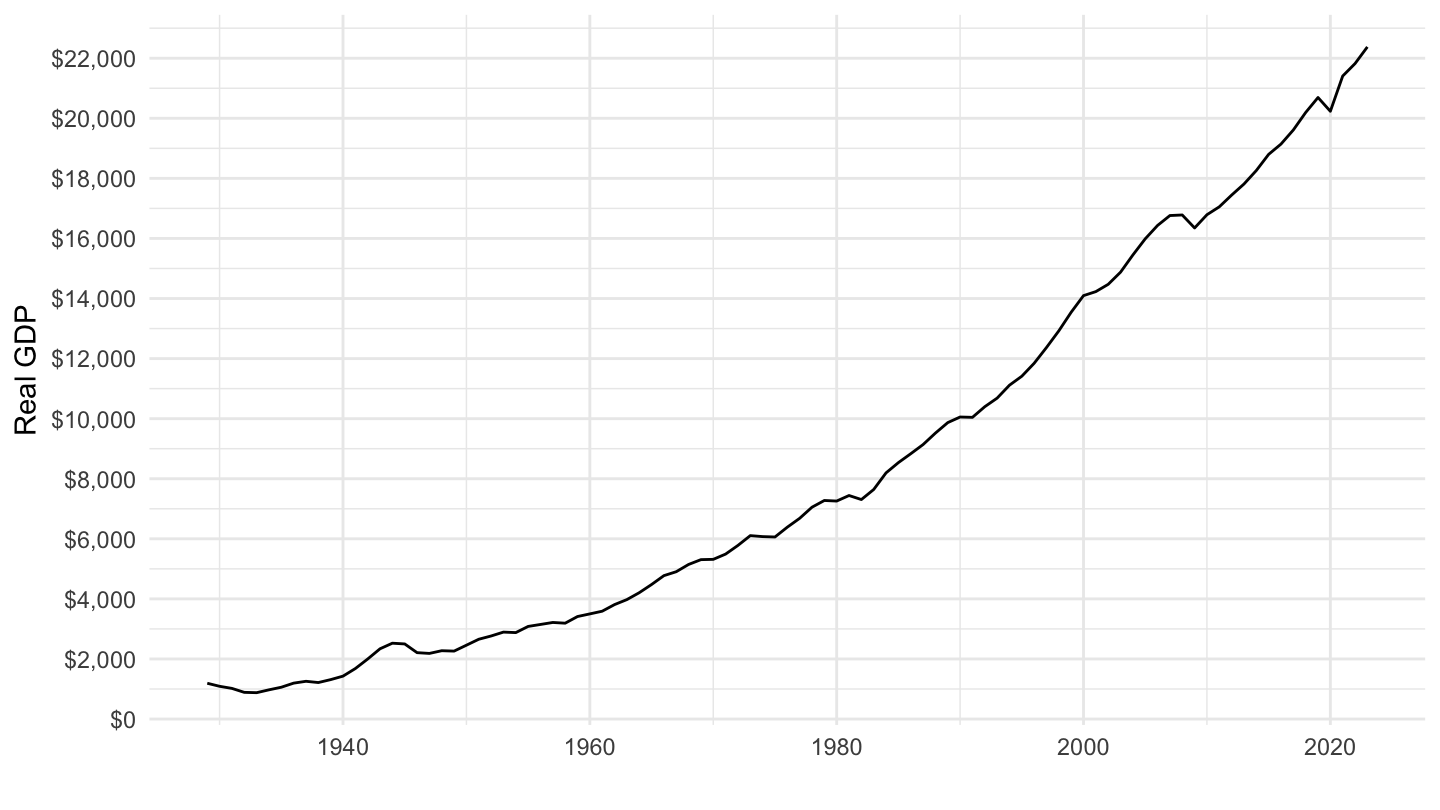

Log

Code

plot_log <- plot_linear +
  scale_y_log10(breaks = seq(0, 100000, 2000),
                     labels = dollar_format(acc = 1))

plot_log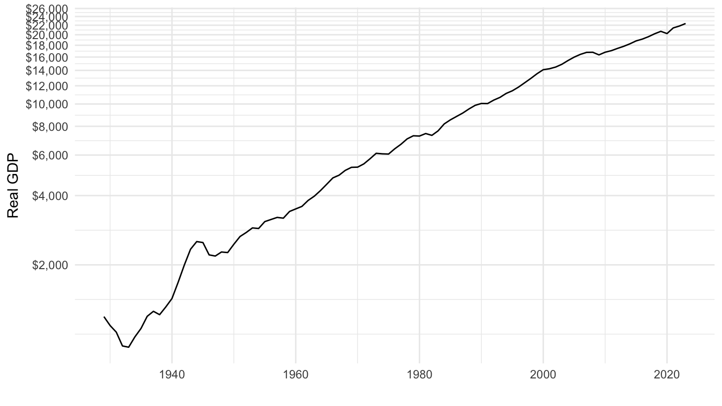

Linear, Log

Code

ggarrange(plot_linear + ggtitle("Linear Scale"), plot_log + ylab("") + ggtitle("Log Scale"))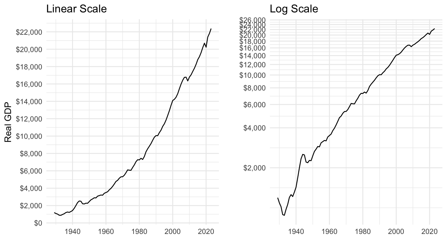

Quarterly

Linear

Code

plot_linear <- gdp %>%
  filter(variable == "GDPC1") %>%
  ggplot + geom_line(aes(x = date, y = value)) +
  scale_y_continuous(breaks = seq(0, 100000, 2000),
                     labels = dollar_format()) +
  scale_x_date(breaks = seq(1950, 2100, 10) %>% paste0("-01-01") %>% as.Date,
               labels = date_format("%Y")) +
  theme_minimal() + xlab("") + ylab("Real GDP")

plot_linear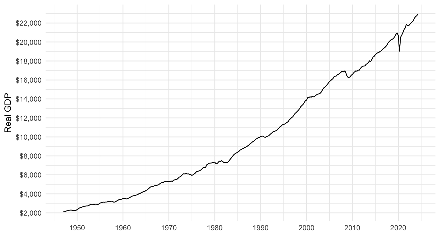

Log

Code

plot_log <- plot_linear +
  scale_y_log10(breaks = seq(0, 100000, 2000),
                     labels = dollar_format(acc = 1))

plot_log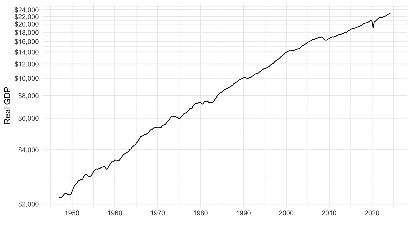

Linear, Log

Code

ggarrange(plot_linear, plot_log + ylab(""))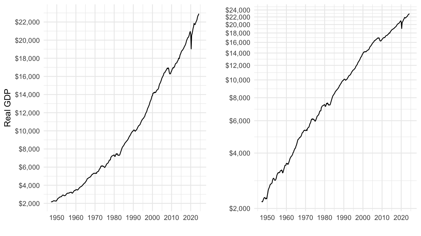

Real GDP per capita

Linear

Code

plot_linear <- gdp %>%
  filter(variable == "A939RX0Q048SBEA") %>%
  ggplot + geom_line(aes(x = date, y = value)) +
  scale_y_continuous(breaks = seq(0, 100000, 10000),
                     labels = dollar_format()) +
  scale_x_date(breaks = seq(1950, 2100, 10) %>% paste0("-01-01") %>% as.Date,
               labels = date_format("%Y")) +
  theme_minimal() + xlab("") + ylab("Real GDP per capita")

plot_linear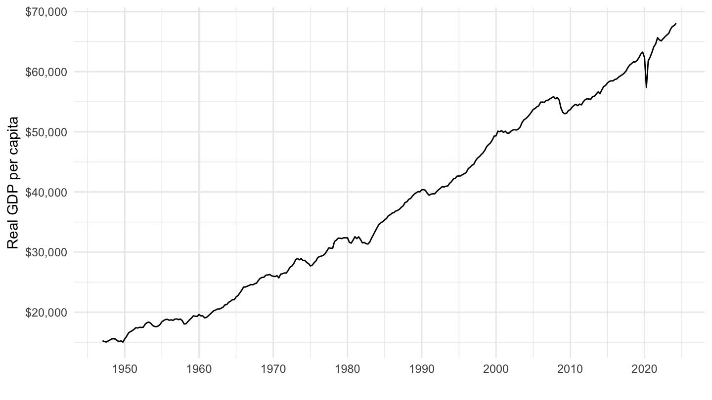

Log

Code

plot_log <- plot_linear +
  scale_y_log10(breaks = seq(0, 100000, 10000),
                     labels = dollar_format(acc = 1))

plot_log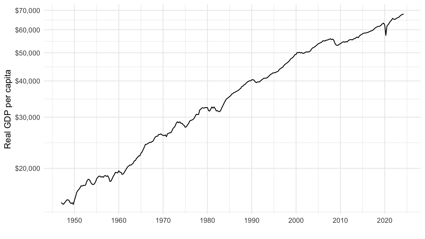

Linear, Log

Code

ggarrange(plot_linear, plot_log + ylab(""))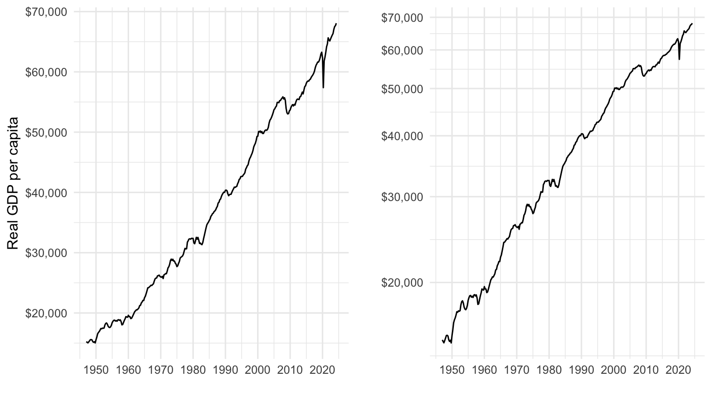

Output Gap (%)

1945-2020

Code

gdp %>%
  spread(variable, value) %>%
  mutate(output_gap = (GDPC1 - GDPPOT)/GDPPOT) %>%
  select(date, output_gap) %>%
  na.omit %>%
  ggplot(.) + xlab("") + ylab("Output Gap (% of Potential Output)") +
  theme_minimal() +
  geom_line(aes(x = date, y = output_gap)) +
  geom_rect(data = nber_recessions %>%
              filter(Peak > as.Date("1948-01-01")), 
            aes(xmin = Peak, xmax = Trough, ymin = -Inf, ymax = +Inf), 
            fill = 'grey', alpha = 0.5) +
  theme(legend.title = element_blank(),
        legend.position = c(0.4, 0.8)) +
  scale_x_date(breaks = as.Date(paste0(seq(1920, 2020, 5), "-01-01")),
               labels = date_format("%Y")) +
  scale_y_continuous(breaks = 0.01*seq(-20, 20, 1),
                     labels = scales::percent_format(accuracy = 1))

1965-2020

Code

gdp %>%
  filter(date >= as.Date("1965-01-01")) %>%
  spread(variable, value) %>%
  mutate(output_gap = (GDPC1 - GDPPOT)/GDPPOT) %>%
  select(date, output_gap) %>%
  na.omit %>%
  ggplot(.) + xlab("") + ylab("Output Gap (% of Potential Output)") +
  theme_minimal() +
  geom_line(aes(x = date, y = output_gap)) +
  geom_rect(data = nber_recessions %>%
              filter(Peak > as.Date("1965-01-01")), 
            aes(xmin = Peak, xmax = Trough, ymin = -Inf, ymax = +Inf), 
            fill = 'grey', alpha = 0.5) +
  theme(legend.title = element_blank(),
        legend.position = c(0.4, 0.8)) +
  scale_x_date(breaks = as.Date(paste0(seq(1920, 2025, 5), "-01-01")),
               labels = date_format("%Y")) +
  scale_y_continuous(breaks = 0.01*seq(-20, 20, 1),
                     labels = scales::percent_format(accuracy = 1))

Deficits

All

(ref:surplus-gdp-1929-2019) Budget Surplus, 1929-2019 (% of GDP).

Code

US_presidents_extract <- US_presidents %>%
  filter(start >= as.Date("1929-01-01"))
gdp %>%
  filter(variable %in% c("FYFSD", "GDPA")) %>%
  mutate(date = date %>% year,
         date = as.Date(paste0(date, "-12-31"))) %>%
  spread(variable, value) %>%
  mutate(value = FYFSD / (GDPA*1000)) %>%
  filter(date >= as.Date("1929-01-01")) %>%
  ggplot(.) + 
  geom_line(aes(x = date, y = value)) + theme_minimal() +
  theme(legend.title = element_blank(),
        legend.position = c(0.3, 0.8)) +
  scale_x_date(breaks = as.Date(US_presidents_extract$start),
               labels = date_format("%Y")) +
  geom_vline(aes(xintercept = as.numeric(start)), 
             data = US_presidents_extract,
             colour = "grey50", alpha = 0.5) +
  geom_rect(aes(xmin = start, xmax = end, fill = party),
         ymin = -Inf, ymax = Inf, alpha = 0.1, data = US_presidents_extract) +
  geom_text(aes(x = start, y = new, label = name), 
            data = US_presidents_extract %>% mutate(new = -0.27 + 0.01 * (1:n() %% 2)),
            size = 2.5, vjust = 0, hjust = 0, nudge_x = 50) +
  # scale_fill_manual(values = viridis(3)[2:1]) +
  scale_fill_manual(values = c("white", "grey")) +
  xlab("") + ylab("Budget Surplus (% of GDP)") +
  guides(color = guide_legend("party"), fill = FALSE) +
  scale_y_continuous(breaks = 0.01*seq(-30, 6, 2),
                     labels = scales::percent_format(accuracy = 1),
                     limits = c(-0.27, 0.05)) + 
  geom_hline(yintercept = 0, linetype = "dashed",  color = viridis(3)[2])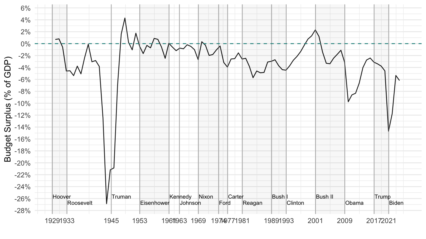

1945-2021

Code

gdp %>%
  filter(variable %in% c("FYFSD", "GDPA")) %>%
  mutate(date = date %>% year,
         date = as.Date(paste0(date, "-12-31"))) %>%
  spread(variable, value) %>%
  mutate(value = FYFSD / (GDPA*1000)) %>%
  ggplot(.) + 
  geom_line(aes(x = date, y = value)) + theme_minimal() +
  theme(legend.title = element_blank(),
        legend.position = c(0.3, 0.8)) +
  scale_x_date(breaks = as.Date(US_presidents$start),
               labels = date_format("%Y"),
               limits = c(as.Date("1929-01-01"), as.Date("2023-04-01"))) +
  geom_vline(aes(xintercept = as.numeric(start)), 
             data = US_presidents,
             colour = "grey50", alpha = 0.5) +
  geom_rect(aes(xmin = start, xmax = end, fill = party),
         ymin = -Inf, ymax = Inf, alpha = 0.1, data = US_presidents) +
  geom_text(aes(x = start, y = new, label = name), 
            data = US_presidents %>% mutate(new = -0.27 + 0.01 * (1:n() %% 2)),
            size = 2.5, vjust = 0, hjust = 0, nudge_x = 50) +
  # scale_fill_manual(values = viridis(3)[2:1]) +
  scale_fill_manual(values = c("white", "grey")) +
  xlab("") + ylab("Budget Surplus (% of GDP)") +
  guides(color = guide_legend("party"), fill = FALSE) +
  scale_y_continuous(breaks = 0.01*seq(-30, 6, 2),
                     labels = scales::percent_format(accuracy = 1),
                     limits = c(-0.27, 0.05)) + 
  geom_hline(yintercept = 0, linetype = "dashed",  color = viridis(3)[2])

Financial Crisis Macroeconomic Aggregates

Household Debt to GDP (% of GDP)

(ref:HDTGPDUSQ163N) Mortgage Debt Service Payments, in Billions (2000-2012)

Code

gdp %>%
  filter(variable == "HDTGPDUSQ163N") %>%
  spread(variable, value) %>%
  na.omit %>%
  mutate(value = HDTGPDUSQ163N / 100) %>% 
  select(date, value) %>%
  filter(date >= as.Date("2000-01-01"), 
         date <= as.Date("2012-01-01")) %>%
  ggplot(.) + geom_line(aes(x = date, y = value)) + theme_minimal() +
  scale_x_date(breaks = seq(1870, 2020, 1) %>% paste0("-01-01") %>% as.Date,
               labels = date_format("%Y")) + 
  scale_y_continuous(breaks = 0.01* seq(10, 120, 1),
                     labels = percent_format(accuracy = 1)) + 
  xlab("") + ylab("Household Debt (% of GDP)") + 
  geom_vline(xintercept = as.Date("2008-09-15"), linetype = "dashed", color = viridis(3)[2]) + 
    geom_rect(data = data_frame(start = as.Date("2004-06-01"), 
                                end = as.Date("2007-08-01")), 
              aes(xmin = start, xmax = end, ymin = -Inf, ymax = +Inf), 
              fill = viridis(4)[4], alpha = 0.2) +
    geom_vline(xintercept = as.Date("2004-06-01"), linetype = "dashed", color = viridis(4)[4]) + 
    geom_vline(xintercept = as.Date("2007-08-01"), linetype = "dashed", color = viridis(4)[4])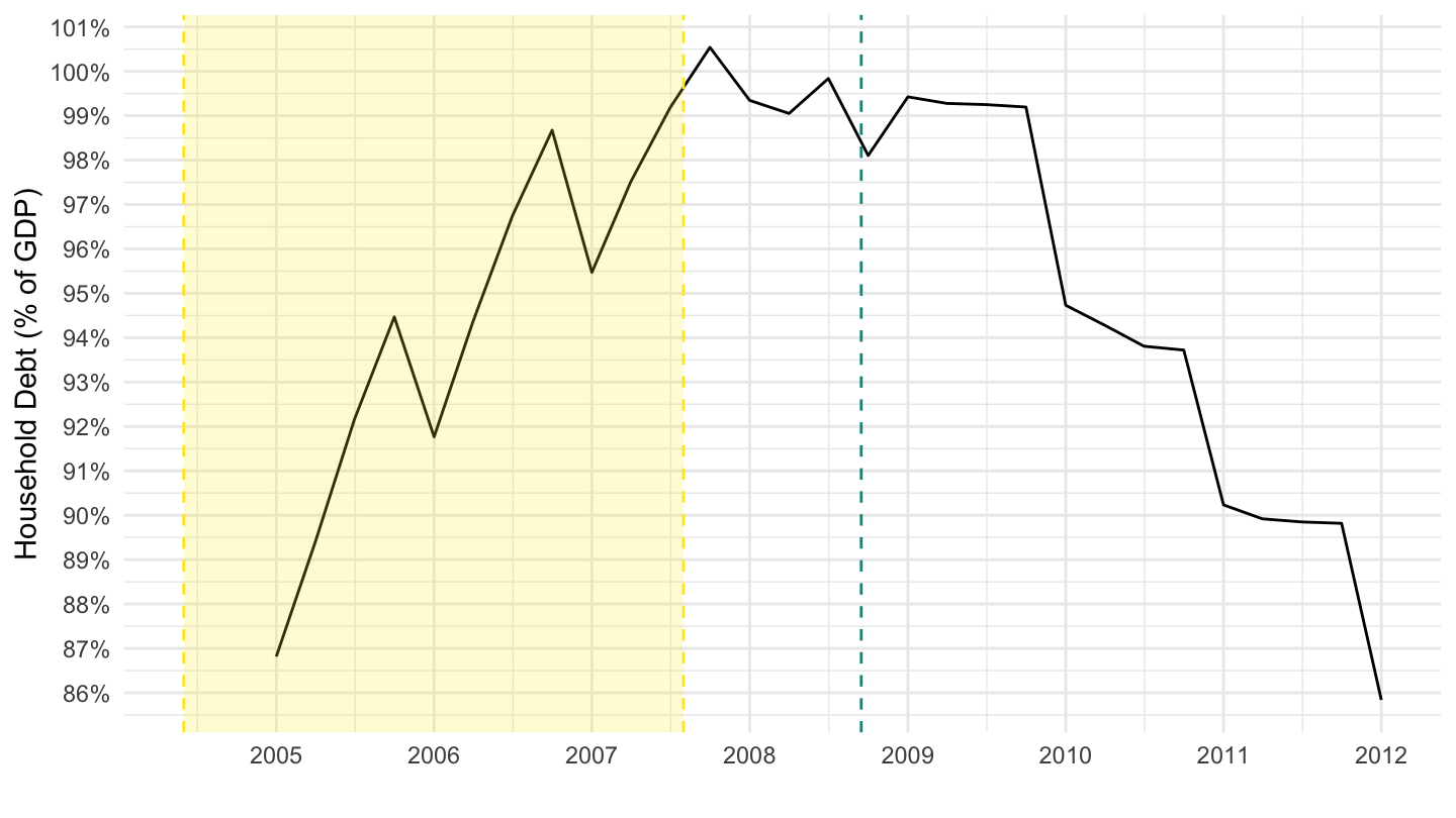

Mortgage Debt Service Payments (in Billion Dollars)

(ref:MDSP-DSPI) Mortgage Debt Service Payments, in Billions (2000-2012)

Code

gdp %>%
  filter(variable %in% c("DSPI", "MDSP")) %>%
  spread(variable, value) %>%
  na.omit %>%
  mutate(value = MDSP * DSPI / 100) %>% 
  select(date, value) %>%
  filter(date >= as.Date("2000-01-01"), 
         date <= as.Date("2012-01-01")) %>%
  ggplot(.) + geom_line(aes(x = date, y = value)) + theme_minimal() +
  scale_x_date(breaks = seq(1870, 2020, 1) %>% paste0("-01-01") %>% as.Date,
               labels = date_format("%Y")) + 
  scale_y_continuous(breaks = seq(100, 16000, 50),
                     labels = dollar_format(suffix = "Bn", prefix = "$")) + 
  xlab("") + ylab("Mortgage Debt Service Payments") + 
  geom_vline(xintercept = as.Date("2008-09-15"), linetype = "dashed", color = viridis(3)[2]) + 
    geom_rect(data = data_frame(start = as.Date("2004-06-01"), 
                                end = as.Date("2007-08-01")), 
              aes(xmin = start, xmax = end, ymin = -Inf, ymax = +Inf), 
              fill = viridis(4)[4], alpha = 0.2) +
    geom_vline(xintercept = as.Date("2004-06-01"), linetype = "dashed", color = viridis(4)[4]) + 
    geom_vline(xintercept = as.Date("2007-08-01"), linetype = "dashed", color = viridis(4)[4])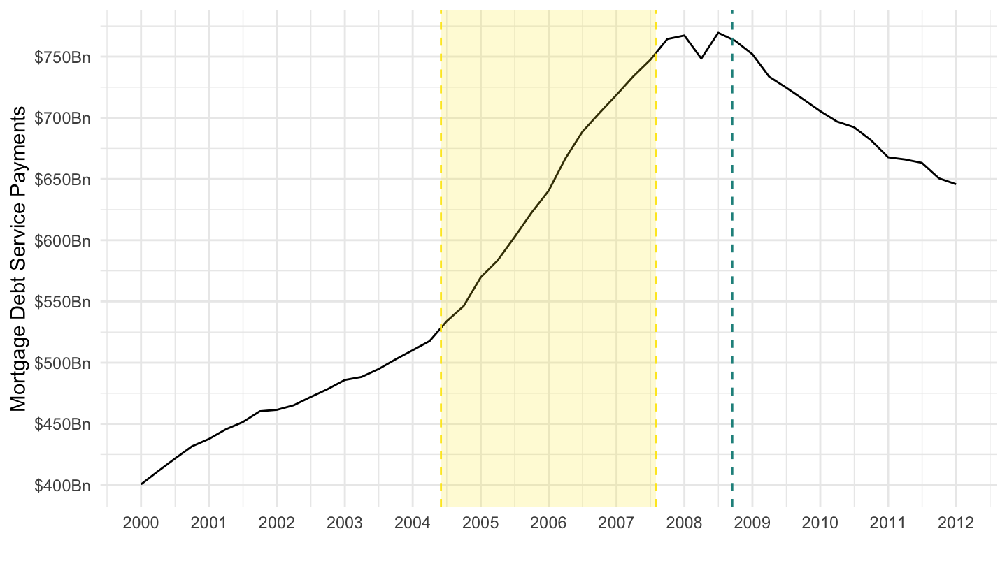

Mortgage Debt Service Payments (% Disposable Personal Income)

(ref:MDSP) Mortgage Debt Service Payments (2000-2019)

Code

gdp %>%
  filter(variable %in% c("MDSP")) %>%
  filter(date >= as.Date("2000-01-01"), 
         date <= as.Date("2012-01-01")) %>%
  mutate(value = value / 100) %>%
  ggplot(.) + geom_line(aes(x = date, y = value)) + theme_minimal() +
  scale_x_date(breaks = seq(1870, 2020, 1) %>% paste0("-01-01") %>% as.Date,
               labels = date_format("%Y")) + 
  scale_y_continuous(breaks = 0.01*seq(0, 15, 0.2),
                     labels = scales::percent_format(accuracy = 0.1)) + 
  xlab("") + ylab("% of Disposable Income") + 
  geom_vline(xintercept = as.Date("2008-09-15"), linetype = "dashed", color = viridis(3)[2]) + 
    geom_rect(data = data_frame(start = as.Date("2004-06-01"), 
                                end = as.Date("2007-08-01")), 
              aes(xmin = start, xmax = end, ymin = -Inf, ymax = +Inf), 
              fill = viridis(4)[4], alpha = 0.2) +
    geom_vline(xintercept = as.Date("2004-06-01"), linetype = "dashed", color = viridis(4)[4]) + 
    geom_vline(xintercept = as.Date("2007-08-01"), linetype = "dashed", color = viridis(4)[4])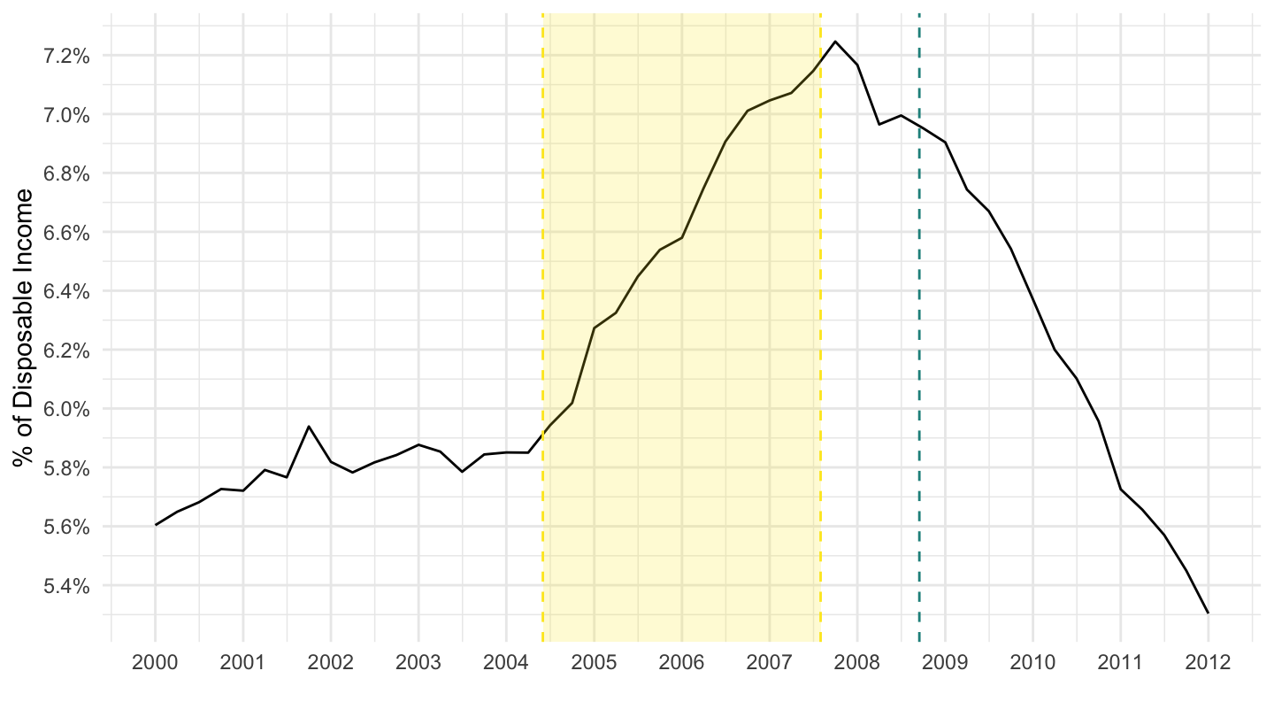

House Prices

(ref:USSTHPI) House Prices (Index)

Code

gdp %>%
  filter(variable %in% c("USSTHPI")) %>%
  filter(date >= as.Date("2000-01-01"), 
         date <= as.Date("2010-01-01")) %>%
  ggplot(.) + geom_line(aes(x = date, y = value)) + theme_minimal() +
  scale_x_date(breaks = seq(1870, 2020, 1) %>% paste0("-01-01") %>% as.Date,
               labels = date_format("%Y")) + 
  scale_y_continuous(breaks = seq(0, 600, 10)) + 
  xlab("") + ylab("House Price Index") + 
  geom_vline(xintercept = as.Date("2008-09-15"), linetype = "dashed", color = viridis(3)[2]) + 
    geom_rect(data = data_frame(start = as.Date("2004-06-01"), 
                                end = as.Date("2007-08-01")), 
              aes(xmin = start, xmax = end, ymin = -Inf, ymax = +Inf), 
              fill = viridis(4)[4], alpha = 0.2) +
    geom_vline(xintercept = as.Date("2004-06-01"), linetype = "dashed", color = viridis(4)[4]) + 
    geom_vline(xintercept = as.Date("2007-08-01"), linetype = "dashed", color = viridis(4)[4])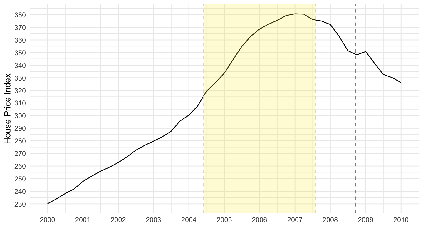

Disposable Income

(ref:DSPI-3) Disposable Income (2000-2019)

Code

gdp %>%
  filter(variable %in% c("DSPI")) %>%
  filter(date >= as.Date("2004-01-01"), 
         date <= as.Date("2010-01-01")) %>%
  ggplot(.) + geom_line(aes(x = date, y = value)) + theme_minimal() +
  scale_x_date(breaks = seq(1870, 2020, 1) %>% paste0("-01-01") %>% as.Date,
               labels = date_format("%Y")) + 
  scale_y_continuous(breaks = seq(6000, 16000, 500),
                     labels = dollar_format(suffix = "Bn", prefix = "$")) + 
  xlab("") + ylab("Disposable Income") + 
  geom_vline(xintercept = as.Date("2008-09-15"), linetype = "dashed", color = viridis(3)[2]) + 
    geom_rect(data = data_frame(start = as.Date("2004-06-01"), 
                                end = as.Date("2007-08-01")), 
              aes(xmin = start, xmax = end, ymin = -Inf, ymax = +Inf), 
              fill = viridis(4)[4], alpha = 0.2) +
    geom_vline(xintercept = as.Date("2004-06-01"), linetype = "dashed", color = viridis(4)[4]) + 
    geom_vline(xintercept = as.Date("2007-08-01"), linetype = "dashed", color = viridis(4)[4])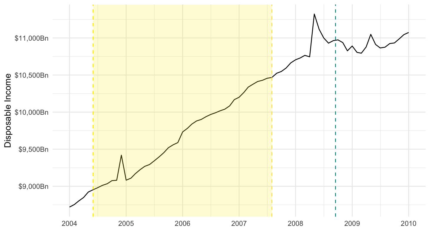

Consumption

Code

gdp %>%
  filter(variable %in% c("PCE")) %>%
  filter(date >= as.Date("2006-01-01"), 
         date <= as.Date("2020-01-01")) %>%
  ggplot(.) + geom_line(aes(x = date, y = value)) + theme_minimal() +
  scale_x_date(breaks = seq(1870, 2020, 1) %>% paste0("-01-01") %>% as.Date,
               labels = date_format("%Y")) + 
  scale_y_continuous(breaks = seq(8000, 20000, 500),
                     labels = dollar_format(suffix = "Bn", prefix = "$")) + 
  xlab("") + ylab("Consumption") + 
  geom_vline(xintercept = as.Date("2008-09-15"), linetype = "dashed", color = viridis(3)[2])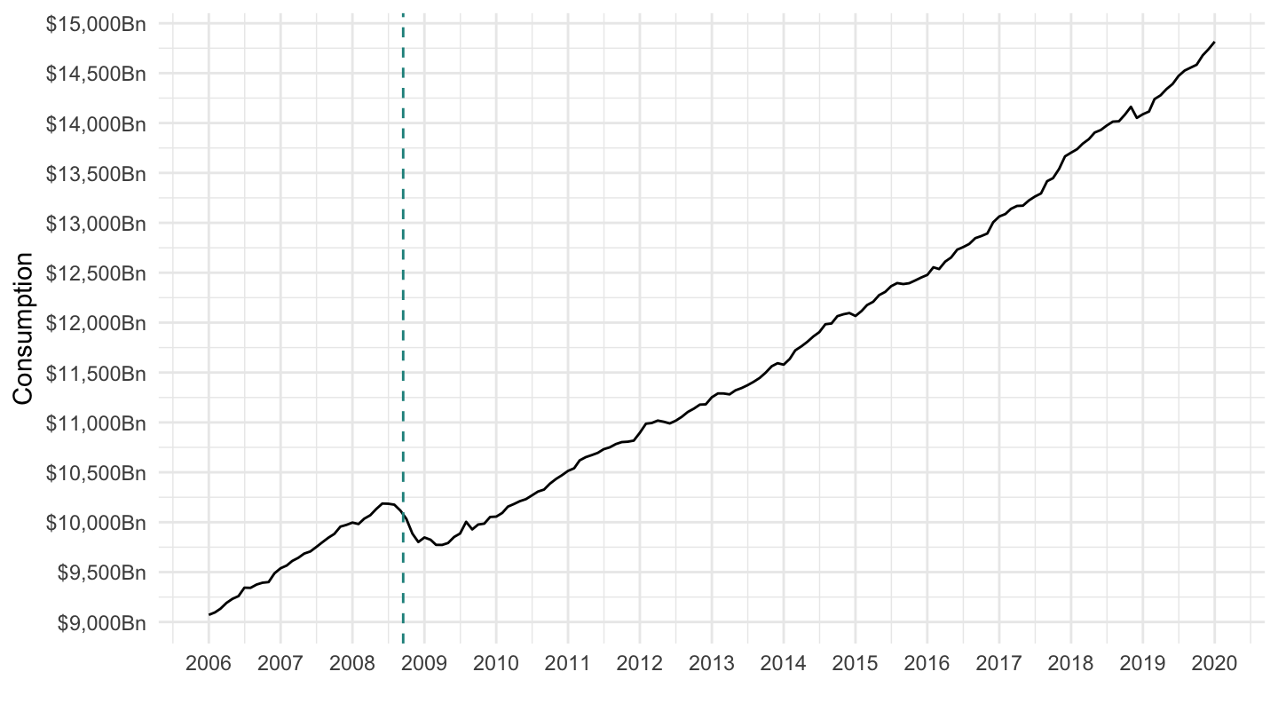

Durable, Non-Durable, Services

(ref:PCND-06-20) Non-durable Expenditures

Code

gdp %>%
  filter(variable %in% c("PCND")) %>%
  filter(date >= as.Date("2006-01-01"), 
         date <= as.Date("2020-01-01")) %>%
  ggplot(.) + geom_line(aes(x = date, y = value)) + theme_minimal() +
  scale_x_date(breaks = seq(1870, 2020, 1) %>% paste0("-01-01") %>% as.Date,
               labels = date_format("%Y")) + 
  scale_y_continuous(breaks = seq(0, 20000, 100),
                     labels = dollar_format(suffix = "Bn", prefix = "$")) + 
  xlab("") + ylab("Non-durable Expenditures") + 
  geom_vline(xintercept = as.Date("2008-09-15"), linetype = "dashed", color = viridis(3)[2])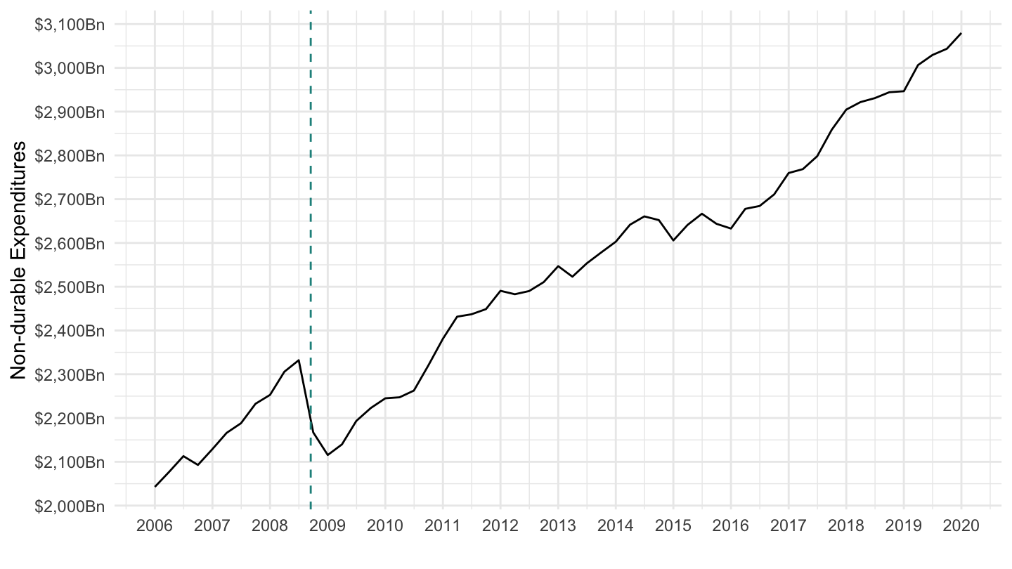

Durable Expenditures

(ref:PCEDG-06-20) Durable Expenditures

Code

gdp %>%
  filter(variable %in% c("PCEDG")) %>%
  filter(date >= as.Date("2001-01-01"), 
         date <= as.Date("2015-01-01")) %>%
  ggplot(.) + geom_line(aes(x = date, y = value)) + theme_minimal() +
  scale_x_date(breaks = seq(1870, 2020, 1) %>% paste0("-01-01") %>% as.Date,
               labels = date_format("%Y")) + 
  scale_y_continuous(breaks = seq(0, 20000, 50),
                     labels = dollar_format(suffix = "Bn", prefix = "$")) + 
  xlab("") + ylab("Durable Expenditures") + 
  geom_vline(xintercept = as.Date("2008-09-15"), linetype = "dashed", color = viridis(3)[2])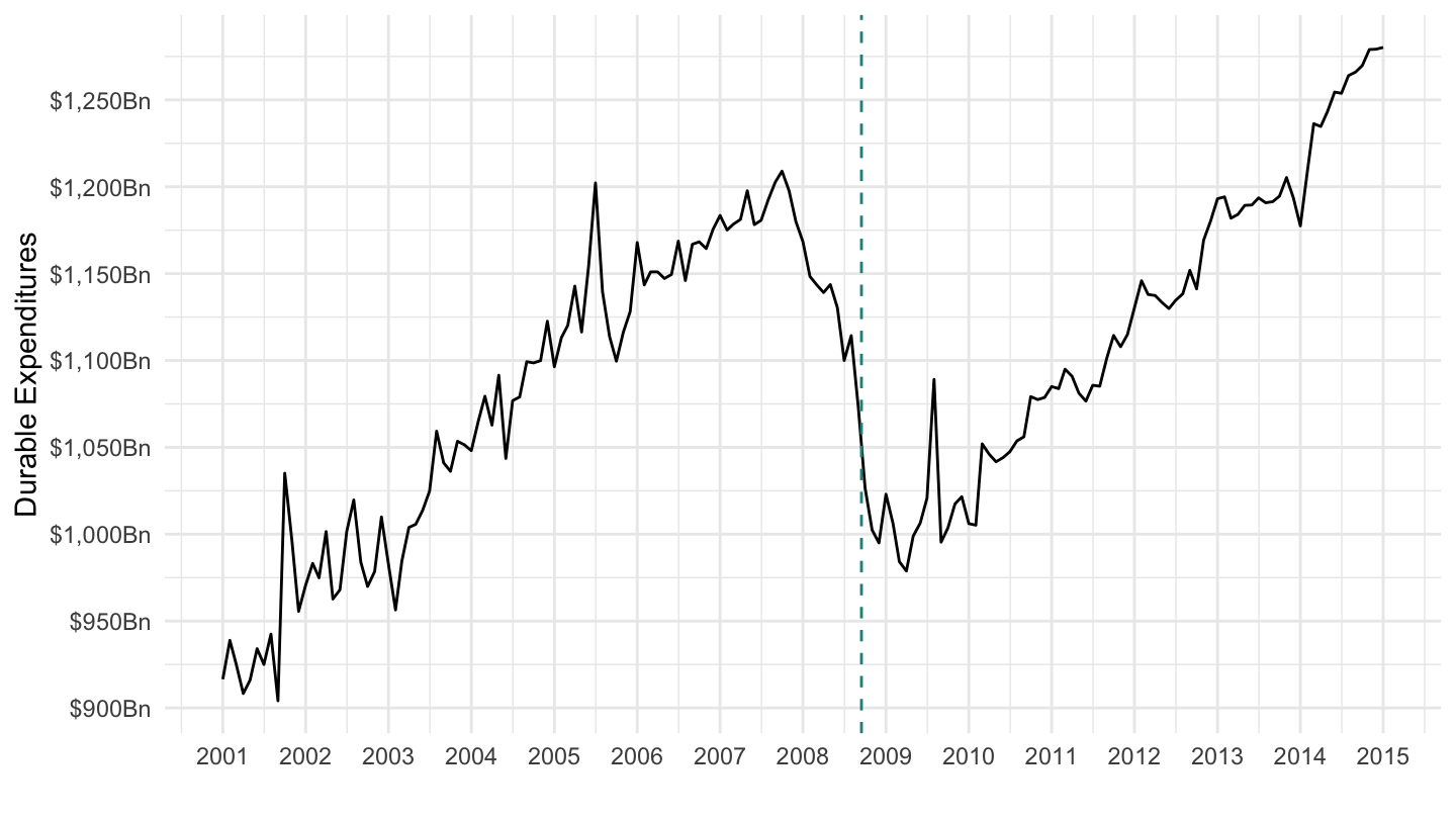

Service Expenditures

(ref:PCESV-06-20) Service Expenditures

Code

gdp %>%
  filter(variable %in% c("PCESV")) %>%
  filter(date >= as.Date("2006-01-01"), 
         date <= as.Date("2020-01-01")) %>%
  ggplot(.) + geom_line(aes(x = date, y = value)) + theme_minimal() +
  scale_x_date(breaks = seq(1870, 2020, 1) %>% paste0("-01-01") %>% as.Date,
               labels = date_format("%Y")) + 
  scale_y_continuous(breaks = 1000*seq(0, 20, 0.5),
                     labels = dollar_format(suffix = "Bn", prefix = "$")) + 
  xlab("") + ylab("Service Expenditures") + 
  geom_vline(xintercept = as.Date("2008-09-15"), linetype = "dashed", color = viridis(3)[2])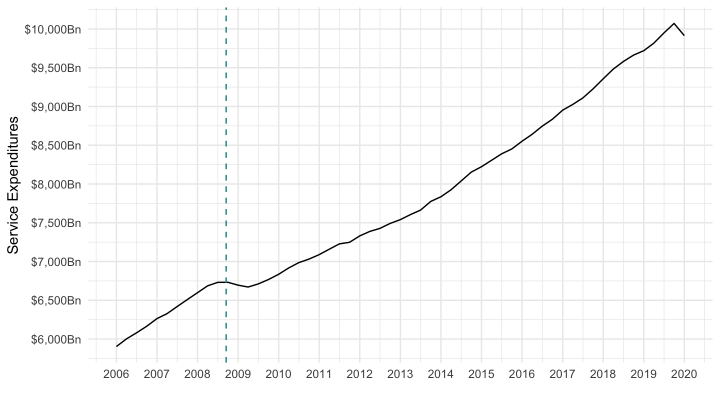

Imputed rental

(ref:DOWNRC1A027NBEA) Imputed rental

Code

gdp %>%
  filter(variable %in% c("DOWNRC1A027NBEA")) %>%
  filter(date >= as.Date("2006-01-01"), 
         date <= as.Date("2020-01-01")) %>%
  ggplot(.) + geom_line(aes(x = date, y = value)) + theme_minimal() +
  scale_x_date(breaks = seq(1870, 2020, 1) %>% paste0("-01-01") %>% as.Date,
               labels = date_format("%Y")) + 
  scale_y_continuous(breaks = seq(0, 20000, 100),
                     labels = dollar_format(suffix = "Bn", prefix = "$")) + 
  xlab("") + ylab("Imputed rental") + 
  geom_vline(xintercept = as.Date("2008-09-15"), linetype = "dashed", color = viridis(3)[2])

Health Care

(ref:USPCEHLTHCARE) Health Care

Code

gdp %>%
  filter(variable %in% c("USPCEHLTHCARE")) %>%
  filter(date >= as.Date("2006-01-01"), 
         date <= as.Date("2020-01-01")) %>%
  mutate(value = value / 10^3) %>%
  ggplot(.) + geom_line(aes(x = date, y = value)) + theme_minimal() +
  scale_x_date(breaks = seq(1870, 2020, 1) %>% paste0("-01-01") %>% as.Date,
               labels = date_format("%Y")) + 
  scale_y_continuous(breaks = seq(0, 20000, 100),
                     labels = dollar_format(suffix = "Bn", prefix = "$")) + 
  xlab("") + ylab("Imputed rental") + 
  geom_vline(xintercept = as.Date("2008-09-15"), linetype = "dashed", color = viridis(3)[2])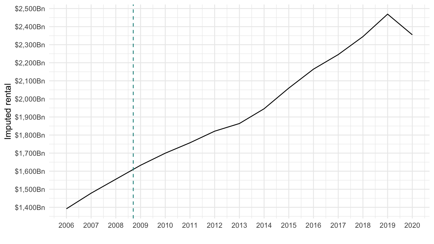

Housing

(ref:DHSGRC0-06-20) Housing

Code

gdp %>%
  filter(variable %in% c("DHSGRC0")) %>%
  filter(date >= as.Date("2006-01-01"), 
         date <= as.Date("2020-01-01")) %>%
  mutate(value = value / 10^3) %>%
  ggplot(.) + geom_line(aes(x = date, y = value)) + theme_minimal() +
  scale_x_date(breaks = seq(1870, 2020, 1) %>% paste0("-01-01") %>% as.Date,
               labels = date_format("%Y")) + 
  scale_y_continuous(breaks = seq(0, 20000, 100),
                     labels = dollar_format(suffix = "Bn", prefix = "$")) + 
  xlab("") + ylab("Housing") + 
  geom_vline(xintercept = as.Date("2008-09-15"), linetype = "dashed", color = viridis(3)[2])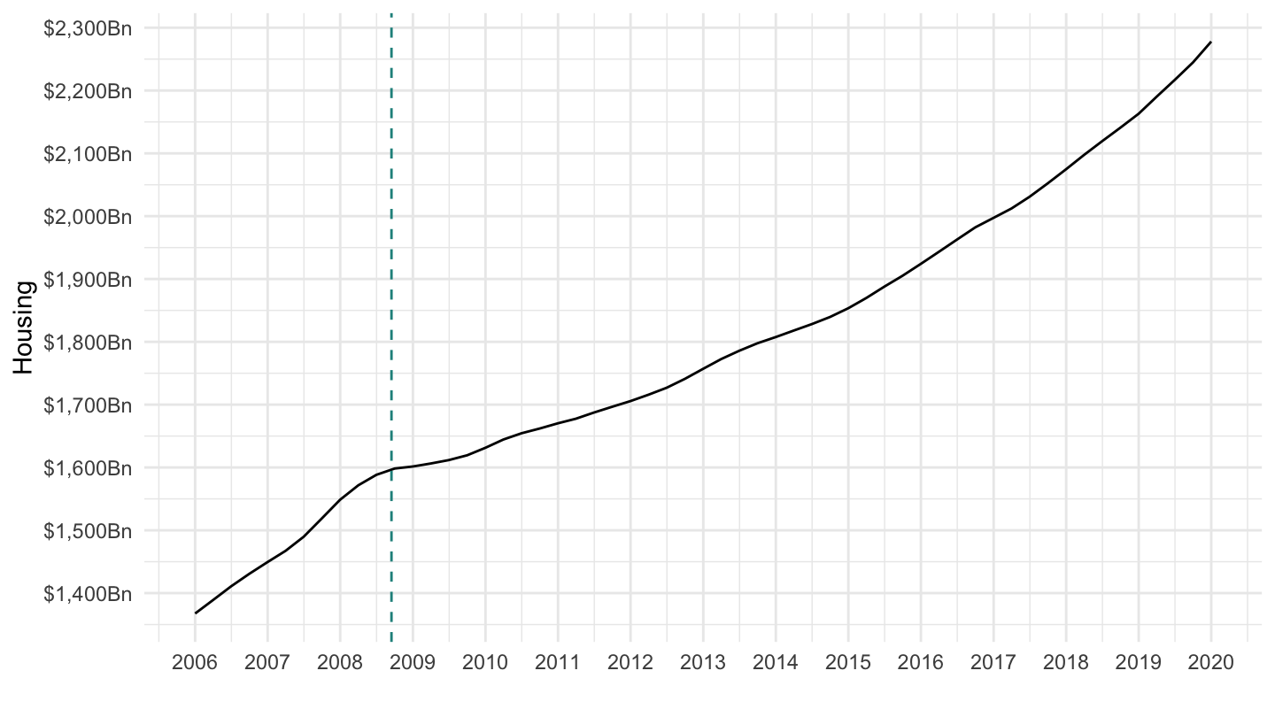

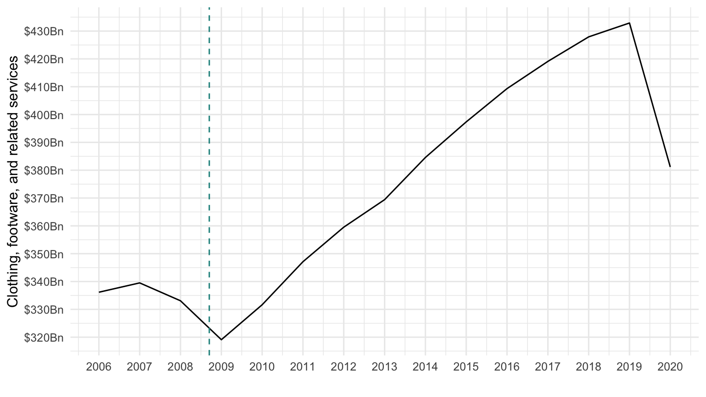
Clothing

(ref:DCAFRC1A027NBEA-06-20) Clothing

Code

gdp %>%
  filter(variable %in% c("DCAFRC1A027NBEA")) %>%
  filter(date >= as.Date("2006-01-01"), 
         date <= as.Date("2020-01-01")) %>%
  mutate(value = value) %>%
  ggplot(.) + geom_line(aes(x = date, y = value)) + theme_minimal() +
  scale_x_date(breaks = seq(1870, 2020, 1) %>% paste0("-01-01") %>% as.Date,
               labels = date_format("%Y")) + 
  scale_y_continuous(breaks = seq(0, 600, 10),
                     labels = dollar_format(suffix = "Bn", prefix = "$")) + 
  xlab("") + ylab("Clothing, footware, and related services") + 
  geom_vline(xintercept = as.Date("2008-09-15"), linetype = "dashed", color = viridis(3)[2])