| source | dataset | Title | .html | .rData |
|---|---|---|---|---|
| wdi | NY.GDP.MKTP.CD | GDP (current USD) | 2026-07-25 | 2026-07-24 |
GDP (current USD)
Data - WDI
Info
Data on macro
| source | dataset | Title | .html | .rData |
|---|---|---|---|---|
| wdi | NY.GDP.MKTP.CD | GDP (current USD) | 2026-07-25 | 2026-07-24 |
| eurostat | nama_10_a10 | Gross value added and income by A*10 industry breakdowns | 2026-07-24 | 2026-07-23 |
| eurostat | nama_10_a10_e | Employment by A*10 industry breakdowns | 2026-07-24 | 2026-07-23 |
| eurostat | nama_10_gdp | GDP and main components (output, expenditure and income) | 2026-07-24 | 2026-07-23 |
| eurostat | nama_10_lp_ulc | Labour productivity and unit labour costs | 2026-07-22 | 2026-07-23 |
| eurostat | namq_10_a10 | Gross value added and income A*10 industry breakdowns | 2026-07-25 | 2026-07-24 |
| eurostat | namq_10_a10_e | Employment A*10 industry breakdowns | 2026-07-24 | 2026-07-24 |
| eurostat | namq_10_gdp | GDP and main components (output, expenditure and income) | 2026-07-24 | 2026-07-23 |
| eurostat | namq_10_lp_ulc | Labour productivity and unit labour costs | 2026-07-24 | 2026-07-24 |
| eurostat | namq_10_pc | Main GDP aggregates per capita | 2026-07-24 | 2026-07-24 |
| eurostat | nasa_10_nf_tr | Non-financial transactions | 2026-07-25 | 2026-07-23 |
| eurostat | nasq_10_nf_tr | Non-financial transactions | 2026-07-25 | 2026-07-23 |
| fred | gdp | Gross Domestic Product | 2026-07-24 | 2026-07-24 |
| oecd | QNA | Quarterly National Accounts | 2026-07-24 | 2026-07-24 |
| oecd | SNA_TABLE1 | Gross domestic product (GDP) | 2026-07-24 | 2025-05-24 |
| oecd | SNA_TABLE14A | Non-financial accounts by sectors | 2026-07-24 | 2024-06-30 |
| oecd | SNA_TABLE2 | Disposable income and net lending - net borrowing | 2024-07-01 | 2024-04-11 |
| oecd | SNA_TABLE6A | Value added and its components by activity, ISIC rev4 | 2024-07-01 | 2024-06-30 |
| wdi | NE.RSB.GNFS.ZS | External balance on goods and services (% of GDP) | 2026-07-25 | 2026-07-24 |
| wdi | NY.GDP.MKTP.PP.CD | GDP, PPP (current international D) | 2026-07-25 | 2026-07-24 |
| wdi | NY.GDP.PCAP.CD | GDP per capita (current USD) | 2026-07-25 | 2026-07-24 |
| wdi | NY.GDP.PCAP.KD | GDP per capita (constant 2015 USD) | 2026-07-25 | 2026-07-24 |
| wdi | NY.GDP.PCAP.PP.CD | GDP per capita, PPP (current international D) | 2026-07-25 | 2026-07-24 |
| wdi | NY.GDP.PCAP.PP.KD | GDP per capita, PPP (constant 2011 international D) | 2026-07-25 | 2026-07-24 |
LAST_COMPILE
| LAST_COMPILE |
|---|
| 2026-07-26 |
Last
Code
NY.GDP.MKTP.CD %>%
  group_by(year) %>%
  summarise(Nobs = n()) %>%
  arrange(desc(year)) %>%
  head(1) %>%
print_table_conditional()| year | Nobs |
|---|---|
| 2025 | 233 |
Nobs - Javascript
Code
NY.GDP.MKTP.CD %>%
left_join(iso2c, by = "iso2c") %>%
group_by(iso2c, Iso2c) %>%
mutate(value = round(value/(10^9))) %>%
summarise(Nobs = n(),
`Year 1` = first(year),
`GDP 1 (Bn)` = first(value) %>% paste0("$ ", .),
`Year 2` = last(year),
`GDP 2 (Bn)` = last(value) %>% paste0("$ ", .)) %>%
arrange(-Nobs) %>%
mutate(Flag = gsub(" ", "-", str_to_lower(Iso2c)),
Flag = paste0('<img src="../../bib/flags/vsmall/', Flag, '.png" alt="Flag">')) %>%
select(Flag, everything()) %>%
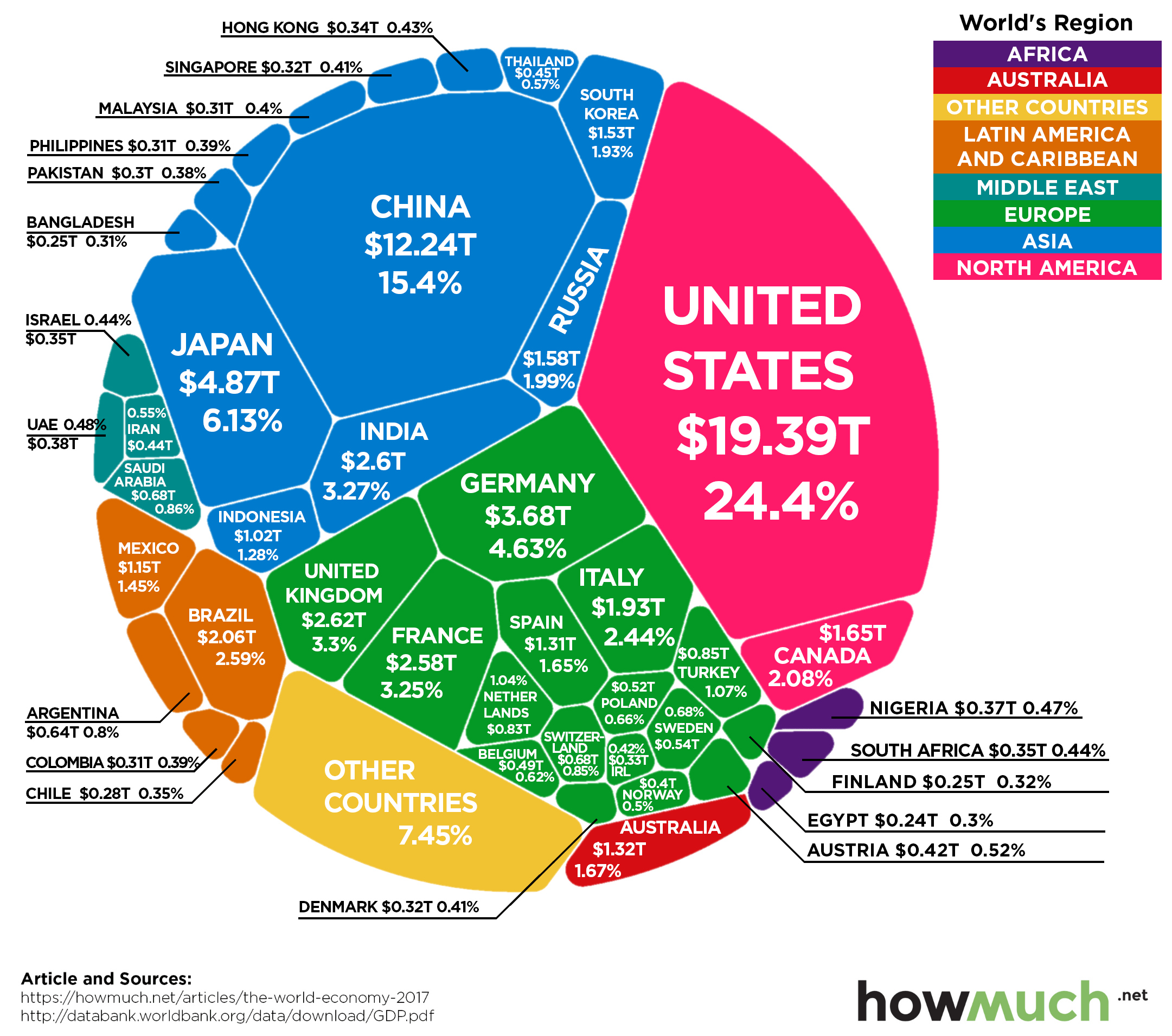
{if (is_html_output()) datatable(., filter = 'top', rownames = F, escape = F) else .}2018 GDP by Country
Code
NY.GDP.MKTP.CD %>%
  right_join(iso2c %>%
              filter((region != "Aggregates") & (region != "NA")),
             by = "iso2c") %>%
  group_by(iso2c, Iso2c) %>%

  mutate(value = round(value/(10^9))) %>%
  summarise(`GDP (Bn)` = last(value)) %>%
  arrange(-`GDP (Bn)`) %>%
  mutate(`GDP (Bn)` = `GDP (Bn)` %>% paste0("$ ", ., " Bn")) %>%
  mutate(Flag = gsub(" ", "-", str_to_lower(Iso2c)),
         Flag = paste0('<img src="../../bib/flags/vsmall/', Flag, '.png" alt="Flag">')) %>%
  select(Flag, everything()) %>%
  {if (is_html_output()) datatable(., filter = 'top', rownames = F, escape = F) else .}
2018 GDP by Country and Aggregates
Code
NY.GDP.MKTP.CD %>%
  right_join(iso2c, by = "iso2c") %>%
  group_by(iso2c, Iso2c) %>%

  mutate(value = round(value/(10^9))) %>%
  summarise(`GDP (Bn)` = last(value)) %>%
  arrange(-`GDP (Bn)`) %>%
  mutate(`GDP (Bn)` = `GDP (Bn)` %>% paste0("$ ", ., " Bn")) %>%
  {if (is_html_output()) datatable(., filter = 'top', rownames = F) else .}
Illustration
Netherlands, Belgium, Switzerland, Turkey, Poland, Sweden
Code
NY.GDP.MKTP.CD %>%
  right_join(iso2c, by = "iso2c") %>%
  filter(iso2c %in% c("1W", "CH", "BE", "NL", "PO", "SE", "TR")) %>%
  year_to_date %>%
  group_by(date) %>%
  mutate(value = value/value[iso2c == "1W"]) %>%
  filter(!(iso2c == "1W")) %>%
  left_join(colors, by = c("Iso2c" = "country")) %>%
  ggplot(.) + theme_minimal() + scale_color_identity() + xlab("") + ylab("% of World GDP") +
  geom_line(aes(x = date, y = value, color = color)) + add_flags +
  scale_x_date(breaks = seq(1950, 2100, 5) %>% paste0("-01-01") %>% as.Date,
               labels = date_format("%Y")) +
  scale_y_continuous(breaks = 0.01*seq(0, 70, 0.2),
                     labels = scales::percent_format(accuracy = .1),
                     limits = 0.01*c(0, 2))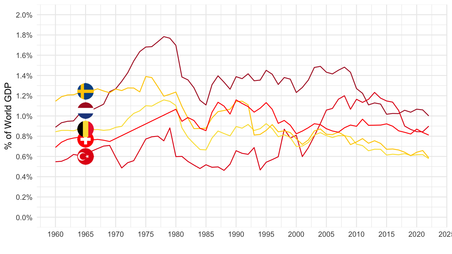
Germany, France, Italy, United Kingdom, Spain
Code
NY.GDP.MKTP.CD %>%
  right_join(iso2c, by = "iso2c") %>%
  filter(iso2c %in% c("1W", "DE", "FR", "IT", "ES", "GB")) %>%
  year_to_date %>%
  group_by(date) %>%
  mutate(value = value/value[iso2c == "1W"]) %>%
  filter(!(iso2c == "1W")) %>%
  left_join(colors, by = c("Iso2c" = "country")) %>%
  ggplot(.) + theme_minimal() + scale_color_identity() + xlab("") + ylab("% of World GDP") +
  geom_line(aes(x = date, y = value, color = color)) + add_flags +
  scale_x_date(breaks = seq(1950, 2100, 5) %>% paste0("-01-01") %>% as.Date,
               labels = date_format("%Y")) +
  scale_y_continuous(breaks = 0.01*seq(0, 70, 2),
                     labels = scales::percent_format(accuracy = 1),
                     limits = 0.01*c(0, 9))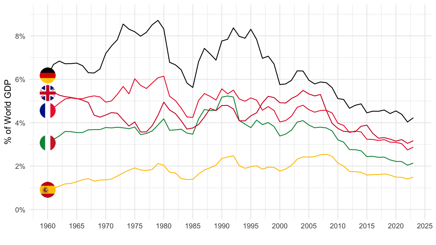
Brazil, Mexico, Argentina
Code
NY.GDP.MKTP.CD %>%
  right_join(iso2c, by = "iso2c") %>%
  filter(iso2c %in% c("1W", "BR", "MX", "AR")) %>%
  year_to_date %>%
  group_by(date) %>%
  mutate(value = value/value[iso2c == "1W"]) %>%
  filter(!(iso2c == "1W")) %>%
  left_join(colors, by = c("Iso2c" = "country")) %>%
  mutate(color = ifelse(iso2c == "MX", color2, color)) %>%
  ggplot(.) + theme_minimal() + scale_color_identity() + xlab("") + ylab("% of World GDP") +
  geom_line(aes(x = date, y = value, color = color)) + add_flags +
  scale_x_date(breaks = seq(1950, 2100, 5) %>% paste0("-01-01") %>% as.Date,
               labels = date_format("%Y")) +
  scale_y_continuous(breaks = 0.01*seq(0, 70, 0.5),
                     labels = scales::percent_format(accuracy = .1),
                     limits = 0.01*c(0, 3.8))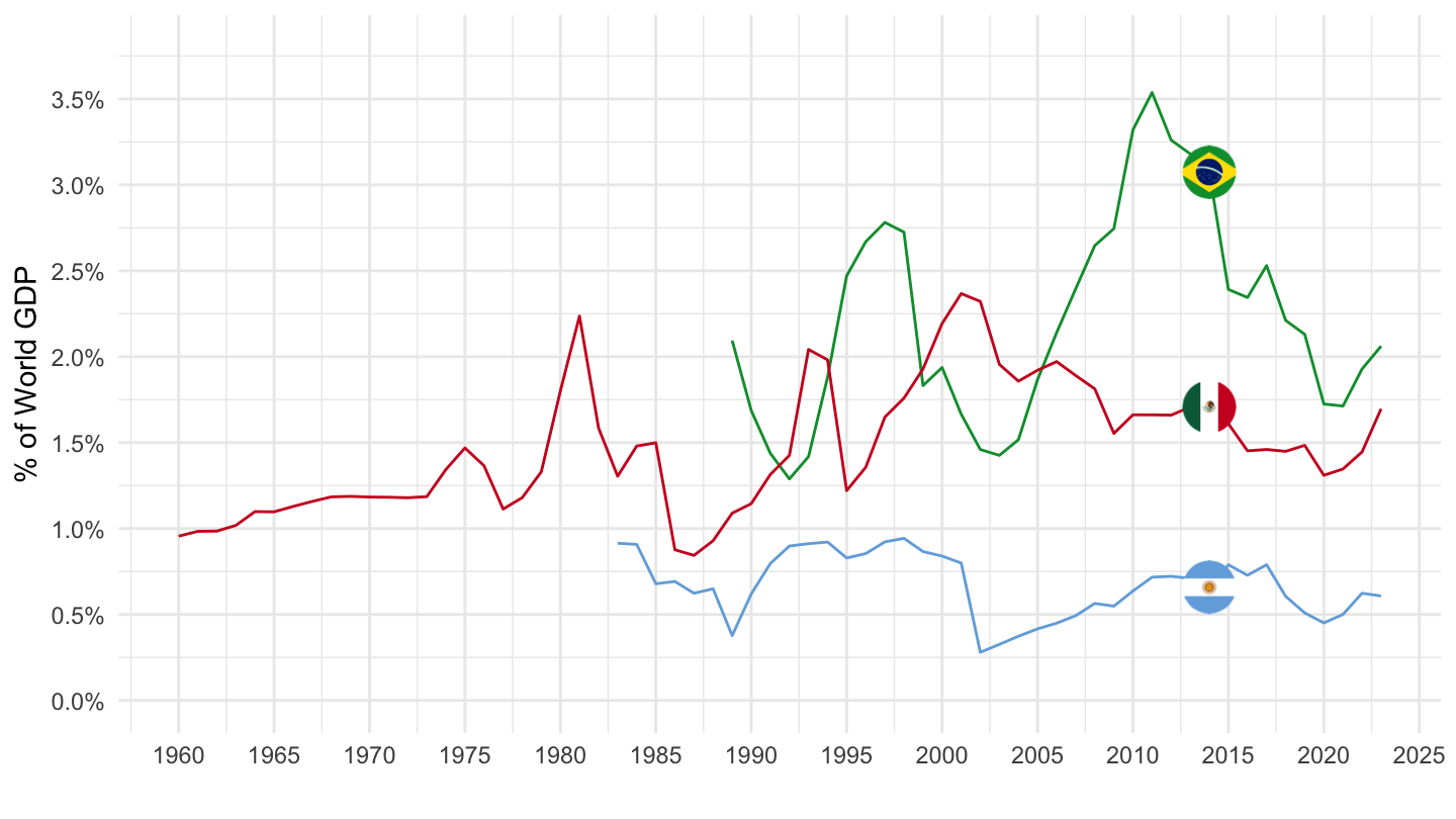
China, E.U., U.S.
All
Code
NY.GDP.MKTP.CD %>%
  right_join(iso2c, by = "iso2c") %>%
  filter(iso2c %in% c("1W", "US", "CN", "EU", "JP")) %>%
  group_by(year) %>%
  mutate(value = value/value[iso2c == "1W"]) %>%
  year_to_date %>%
  filter(!(iso2c == "1W")) %>%
  mutate(Iso2c = ifelse(iso2c == "EU", "Europe", Iso2c)) %>%
  left_join(colors, by = c("Iso2c" = "country")) %>%
  mutate(color = ifelse(iso2c == "US", color2, color)) %>%
  ggplot(.) + theme_minimal() + scale_color_identity() +
  geom_line(aes(x = date, y = value, color = color)) +
  add_flags +
  scale_x_date(breaks = seq(1950, 2100, 5) %>% paste0("-01-01") %>% as.Date,
               labels = date_format("%Y")) +
  scale_y_continuous(breaks = 0.01*seq(0, 70, 5),
                     labels = scales::percent_format(accuracy = 1),
                     limits = 0.01*c(0, 40)) +
  xlab("") + ylab("% du PIB mondial")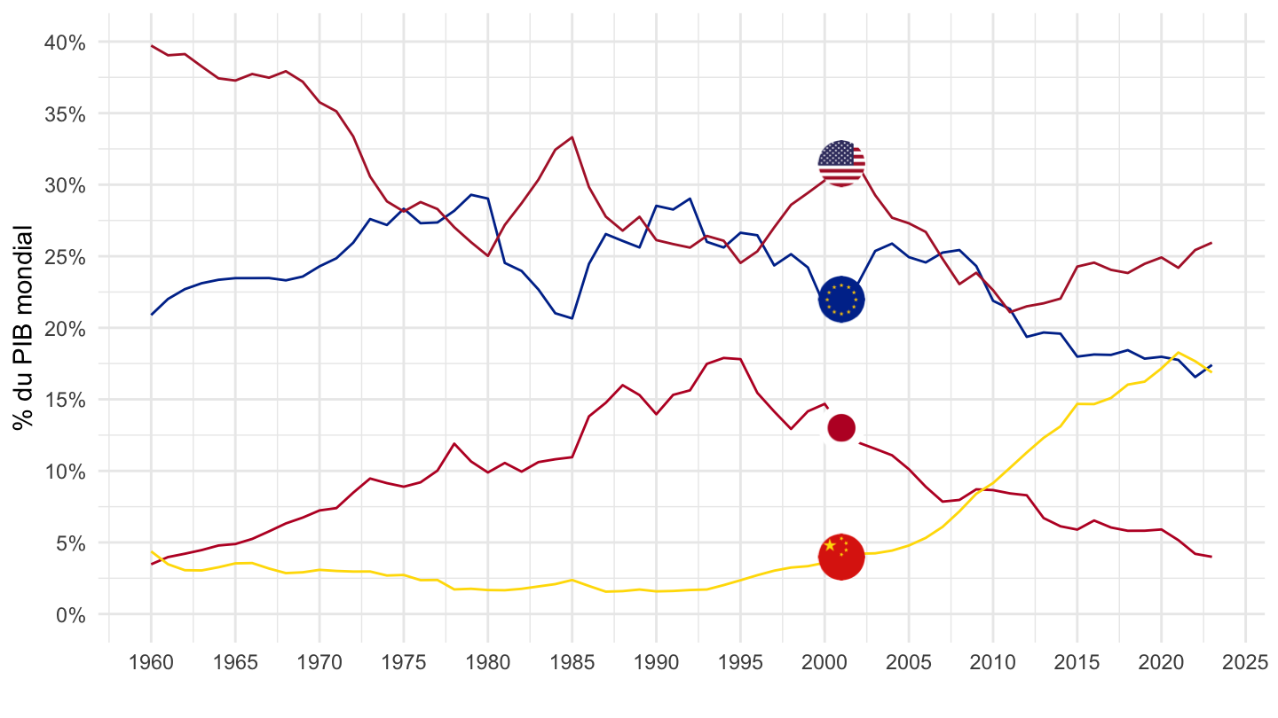
China, E.U., U.S.
All
English
Code
NY.GDP.MKTP.CD %>%
  right_join(iso2c, by = "iso2c") %>%
  filter(iso2c %in% c("1W", "US", "CN", "EU")) %>%
  group_by(year) %>%
  mutate(value = value/value[iso2c == "1W"]) %>%
  year_to_date %>%
  filter(!(iso2c == "1W")) %>%
  mutate(Iso2c = ifelse(iso2c == "EU", "Europe", Iso2c)) %>%
  left_join(colors, by = c("Iso2c" = "country")) %>%
  mutate(color = ifelse(iso2c == "US", color2, color)) %>%
  ggplot(.) + theme_minimal() + scale_color_identity() +
  geom_line(aes(x = date, y = value, color = color)) +
  add_flags +
  scale_x_date(breaks = seq(1950, 2100, 5) %>% paste0("-01-01") %>% as.Date,
               labels = date_format("%Y")) +
  scale_y_continuous(breaks = 0.01*seq(0, 70, 5),
                     labels = scales::percent_format(accuracy = 1),
                     limits = 0.01*c(0, 40)) +
  xlab("") + ylab("% of World GDP")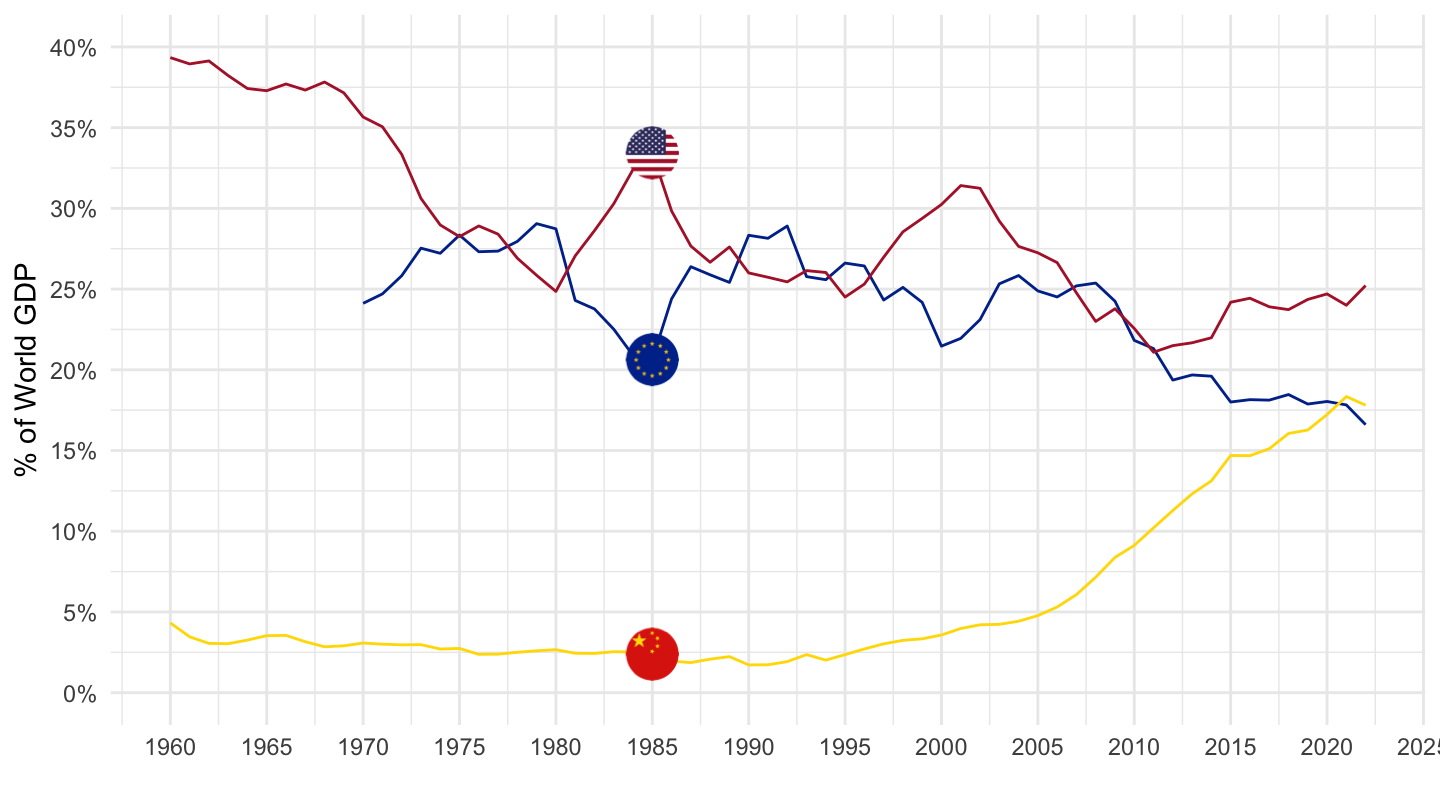
French
Code
NY.GDP.MKTP.CD %>%
  right_join(iso2c, by = "iso2c") %>%
  filter(iso2c %in% c("1W", "US", "CN", "EU")) %>%
  group_by(year) %>%
  mutate(value = value/value[iso2c == "1W"]) %>%
  year_to_date %>%
  filter(!(iso2c == "1W")) %>%
  mutate(Iso2c = ifelse(iso2c == "EU", "Europe", Iso2c)) %>%
  left_join(colors, by = c("Iso2c" = "country")) %>%
  mutate(color = ifelse(iso2c == "US", color2, color)) %>%
  ggplot(.) + theme_minimal() + scale_color_identity() +
  geom_line(aes(x = date, y = value, color = color)) +
  add_flags +
  scale_x_date(breaks = seq(1950, 2100, 5) %>% paste0("-01-01") %>% as.Date,
               labels = date_format("%Y")) +
  scale_y_continuous(breaks = 0.01*seq(0, 70, 5),
                     labels = scales::percent_format(accuracy = 1),
                     limits = 0.01*c(0, 40)) +
  xlab("") + ylab("% du PIB mondial")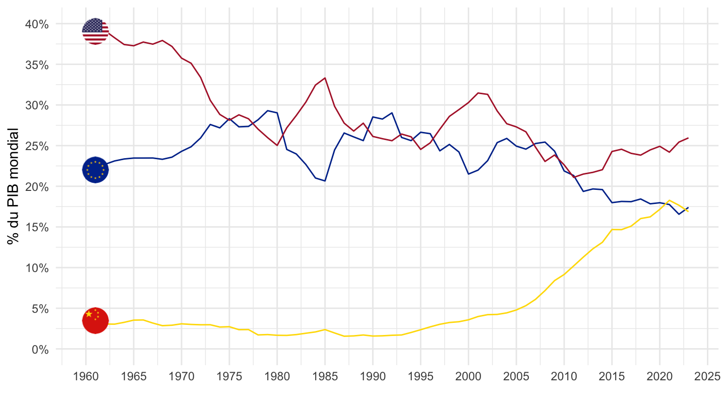
1990-
Code
NY.GDP.MKTP.CD %>%
  right_join(iso2c, by = "iso2c") %>%
  filter(iso2c %in% c("1W", "US", "CN", "EU")) %>%
  group_by(year) %>%
  mutate(value = value/value[iso2c == "1W"]) %>%
  year_to_date %>%
  filter(!(iso2c == "1W")) %>%
  mutate(Iso2c = ifelse(iso2c == "EU", "Europe", Iso2c)) %>%
  filter(date >= as.Date("1990-01-01")) %>%
  left_join(colors, by = c("Iso2c" = "country")) %>%
  mutate(color = ifelse(iso2c == "US", color2, color)) %>%
  ggplot(.) + theme_minimal() + scale_color_identity() +
  geom_line(aes(x = date, y = value, color = color)) +
  add_flags +
  theme(legend.title = element_blank(),
        legend.position = c(0.85, 0.85)) +
  scale_x_date(breaks = seq(1950, 2100, 5) %>% paste0("-01-01") %>% as.Date,
               labels = date_format("%Y")) +
  scale_y_continuous(breaks = 0.01*seq(0, 70, 2),
                     labels = scales::percent_format(accuracy = 1),
                     limits = 0.01*c(0, 35)) +
  xlab("") + ylab("% of World GDP")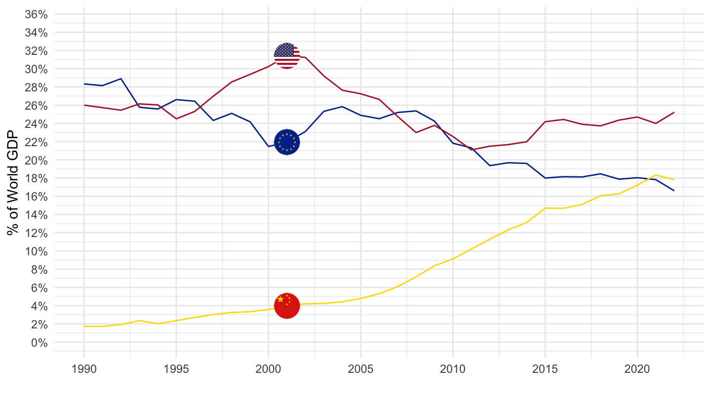
1995-
Code
NY.GDP.MKTP.CD %>%
  right_join(iso2c, by = "iso2c") %>%
  filter(iso2c %in% c("1W", "US", "CN", "EU")) %>%
  group_by(year) %>%
  mutate(value = value/value[iso2c == "1W"]) %>%
  year_to_date %>%
  filter(!(iso2c == "1W")) %>%
  mutate(Iso2c = ifelse(iso2c == "EU", "Europe", Iso2c)) %>%
  filter(date >= as.Date("1995-01-01")) %>%
  left_join(colors, by = c("Iso2c" = "country")) %>%
  mutate(color = ifelse(iso2c != "US", color2, color)) %>%
  ggplot(.) + theme_minimal() + scale_color_identity() +
  geom_line(aes(x = date, y = value, color = color)) +
  add_flags +
  theme(legend.title = element_blank(),
        legend.position = c(0.85, 0.85)) +
  scale_x_date(breaks = seq(1950, 2100, 5) %>% paste0("-01-01") %>% as.Date,
               labels = date_format("%Y")) +
  scale_y_continuous(breaks = 0.01*seq(0, 70, 2),
                     labels = scales::percent_format(accuracy = 1),
                     limits = 0.01*c(0, 35)) +
  xlab("") + ylab("% du PIB mondial")  +
  geom_label_repel(data = . %>% group_by(Iso2c) %>% filter(date %in% c(min(date), max(date))),
                   aes(x = date, y = value, label = percent(value, acc = 0.1), color = color))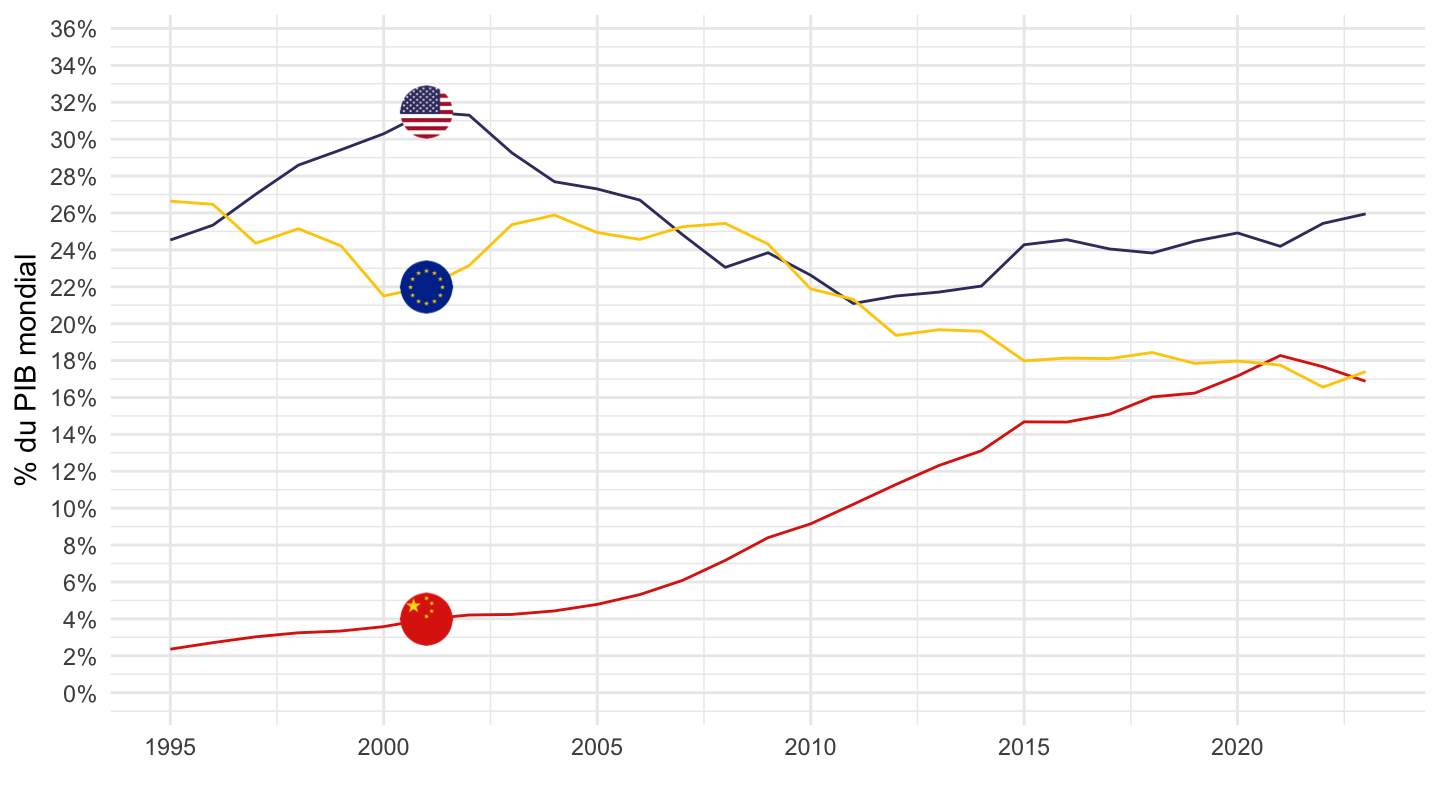
1996-
Code
NY.GDP.MKTP.CD %>%
  right_join(iso2c, by = "iso2c") %>%
  filter(iso2c %in% c("1W", "US", "CN", "EU")) %>%
  group_by(year) %>%
  mutate(value = value/value[iso2c == "1W"]) %>%
  year_to_date %>%
  filter(!(iso2c == "1W")) %>%
  mutate(Iso2c = ifelse(iso2c == "EU", "Europe", Iso2c)) %>%
  filter(date >= as.Date("1996-01-01")) %>%
  left_join(colors, by = c("Iso2c" = "country")) %>%
  mutate(color = ifelse(iso2c != "US", color2, color)) %>%
  ggplot(.) + theme_minimal() + scale_color_identity() +
  geom_line(aes(x = date, y = value, color = color)) +
  add_flags +
  theme(legend.title = element_blank(),
        legend.position = c(0.85, 0.85)) +
  scale_x_date(breaks = seq(1996, 2100, 5) %>% paste0("-01-01") %>% as.Date,
               labels = date_format("%Y")) +
  scale_y_continuous(breaks = 0.01*seq(0, 70, 2),
                     labels = scales::percent_format(accuracy = 1),
                     limits = 0.01*c(0, 35)) +
  xlab("") + ylab("% du PIB mondial")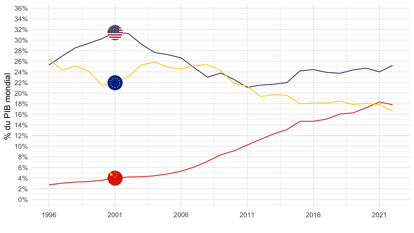
2005-
Code
NY.GDP.MKTP.CD %>%
  right_join(iso2c, by = "iso2c") %>%
  filter(iso2c %in% c("1W", "US", "CN", "EU")) %>%
  group_by(year) %>%
  mutate(value = value/value[iso2c == "1W"]) %>%
  year_to_date %>%
  filter(!(iso2c == "1W")) %>%
  mutate(Iso2c = ifelse(iso2c == "EU", "Europe", Iso2c)) %>%
  filter(date >= as.Date("2005-01-01")) %>%
  left_join(colors, by = c("Iso2c" = "country")) %>%
  mutate(color = ifelse(iso2c == "US", color2, color)) %>%
  ggplot(.) + theme_minimal() + scale_color_identity() +
  geom_line(aes(x = date, y = value, color = color)) +
  add_flags +
  theme(legend.title = element_blank(),
        legend.position = c(0.85, 0.85)) +
  scale_x_date(breaks = seq(1950, 2100, 2) %>% paste0("-01-01") %>% as.Date,
               labels = date_format("%Y")) +
  scale_y_continuous(breaks = 0.01*seq(0, 70, 5),
                     labels = scales::percent_format(accuracy = 1),
                     limits = 0.01*c(0, 30)) +
  xlab("") + ylab("% of World GDP")
Russia, Germany, France
Code
NY.GDP.MKTP.CD %>%
  right_join(iso2c, by = "iso2c") %>%
  filter(iso2c %in% c("1W", "FR", "DE", "RU")) %>%
  group_by(year) %>%
  mutate(value = value/value[iso2c == "1W"]) %>%
  year_to_date %>%
  filter(!(iso2c == "1W")) %>%
  mutate(Iso2c = ifelse(iso2c == "KR", "South Korea", Iso2c)) %>%
  mutate(Iso2c = ifelse(iso2c == "RU", "Russia", Iso2c)) %>%
  left_join(colors, by = c("Iso2c" = "country")) %>%
  mutate(color = ifelse(iso2c == "FR", color2, color)) %>%
  ggplot(.) + theme_minimal() + scale_color_identity() + xlab("") + ylab("% of World GDP") +
  geom_line(aes(x = date, y = value, color = color)) +
  add_flags +
  scale_x_date(breaks = seq(1950, 2100, 5) %>% paste0("-01-01") %>% as.Date,
               labels = date_format("%Y")) +
  scale_y_continuous(breaks = 0.01*seq(0, 70, 1),
                     labels = scales::percent_format(accuracy = 1))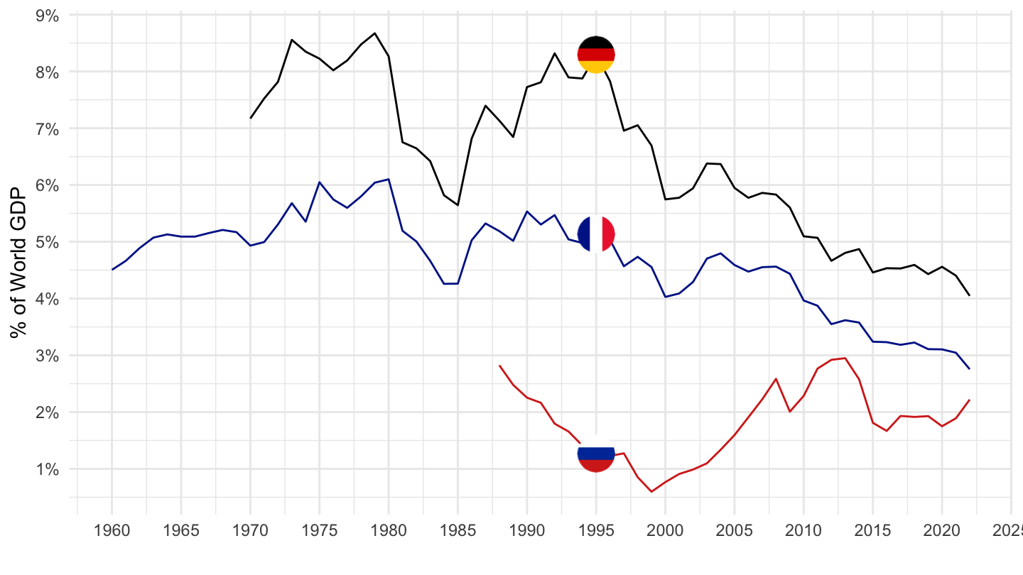
South Korea, Russia, Indonesia
Code
NY.GDP.MKTP.CD %>%
  right_join(iso2c, by = "iso2c") %>%
  filter(iso2c %in% c("1W", "ID", "KR", "RU")) %>%
  group_by(year) %>%
  mutate(value = value/value[iso2c == "1W"]) %>%
  year_to_date %>%
  filter(!(iso2c == "1W")) %>%
  mutate(Iso2c = ifelse(iso2c == "KR", "South Korea", Iso2c)) %>%
  mutate(Iso2c = ifelse(iso2c == "RU", "Russia", Iso2c)) %>%
  left_join(colors, by = c("Iso2c" = "country")) %>%
  ggplot(.) + theme_minimal() + scale_color_identity() + xlab("") + ylab("% of World GDP") +
  geom_line(aes(x = date, y = value, color = color)) +
  add_flags +
  scale_x_date(breaks = seq(1950, 2100, 5) %>% paste0("-01-01") %>% as.Date,
               labels = date_format("%Y")) +
  scale_y_continuous(breaks = 0.01*seq(0, 70, 1),
                     labels = scales::percent_format(accuracy = 1),
                     limits = 0.01*c(0, 4))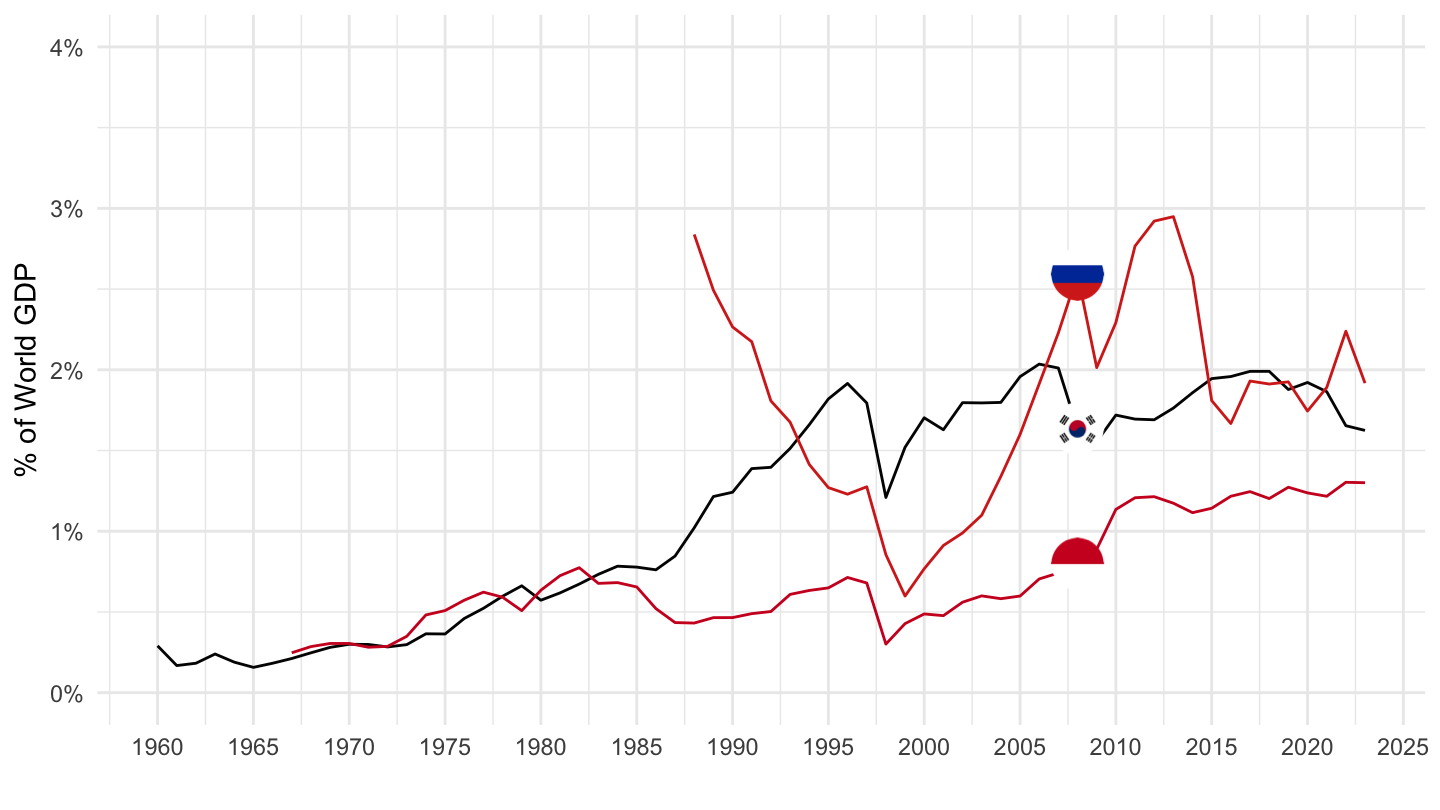
Japan, India, United Kingdom
Code
NY.GDP.MKTP.CD %>%
  right_join(iso2c, by = "iso2c") %>%
  filter(iso2c %in% c("1W", "IN", "JP", "GB")) %>%
  group_by(year) %>%
  mutate(value = value/value[iso2c == "1W"]) %>%
  year_to_date %>%
  filter(!(iso2c == "1W")) %>%
  left_join(colors, by = c("Iso2c" = "country")) %>%
  ggplot(.) + theme_minimal() + scale_color_identity() +
  geom_line(aes(x = date, y = value, color = color)) +
  add_flags +
  theme(legend.title = element_blank(),
        legend.position = c(0.85, 0.85)) +
  scale_x_date(breaks = seq(1950, 2100, 5) %>% paste0("-01-01") %>% as.Date,
               labels = date_format("%Y")) +
  scale_y_continuous(breaks = 0.01*seq(0, 70, 2),
                     labels = scales::percent_format(accuracy = 1),
                     limits = 0.01*c(0, 20)) +
  xlab("") + ylab("% of World GDP")
Germany, France, Italy
Code
NY.GDP.MKTP.CD %>%
  right_join(iso2c, by = "iso2c") %>%
  filter(iso2c %in% c("1W", "DE", "FR", "IT")) %>%
  group_by(year) %>%
  mutate(value = value/value[iso2c == "1W"]) %>%
  year_to_date %>%
  filter(!(iso2c == "1W")) %>%
  left_join(colors, by = c("Iso2c" = "country")) %>%
  ggplot(.) + theme_minimal() + scale_color_identity() +
  geom_line(aes(x = date, y = value, color = color)) +
  add_flags +
  theme(legend.title = element_blank(),
        legend.position = c(0.85, 0.85)) +
  scale_x_date(breaks = seq(1950, 2100, 5) %>% paste0("-01-01") %>% as.Date,
               labels = date_format("%Y")) +
  scale_y_continuous(breaks = 0.01*seq(0, 70, 2),
                     labels = scales::percent_format(accuracy = 1),
                     limits = 0.01*c(0, 10)) +
  xlab("") + ylab("% of World GDP")
United States
All
Code
NY.GDP.MKTP.CD %>%
  right_join(iso2c, by = "iso2c") %>%
  filter(iso2c %in% c("1W", "XC", "US")) %>%
  group_by(year) %>%
  mutate(value = value/value[iso2c == "1W"]) %>%
  year_to_date %>%
  filter(!(iso2c == "1W")) %>%
  mutate(Iso2c = ifelse(iso2c == "XC", "Europe", Iso2c)) %>%
  left_join(colors, by = c("Iso2c" = "country")) %>%
  mutate(color = ifelse(iso2c == "US", color2, color)) %>%
  ggplot(.) + theme_minimal() + scale_color_identity() +
  geom_line(aes(x = date, y = value, color = color)) +
  add_flags +
  theme(legend.title = element_blank(),
        legend.position = c(0.85, 0.85)) +
  scale_x_date(breaks = seq(1950, 2100, 5) %>% paste0("-01-01") %>% as.Date,
               labels = date_format("%Y")) +
  scale_y_continuous(breaks = 0.01*seq(0, 70, 5),
                     labels = scales::percent_format(accuracy = 1)) +
  xlab("") + ylab("% of World GDP") +
  geom_vline(xintercept = as.Date("1980-01-01"))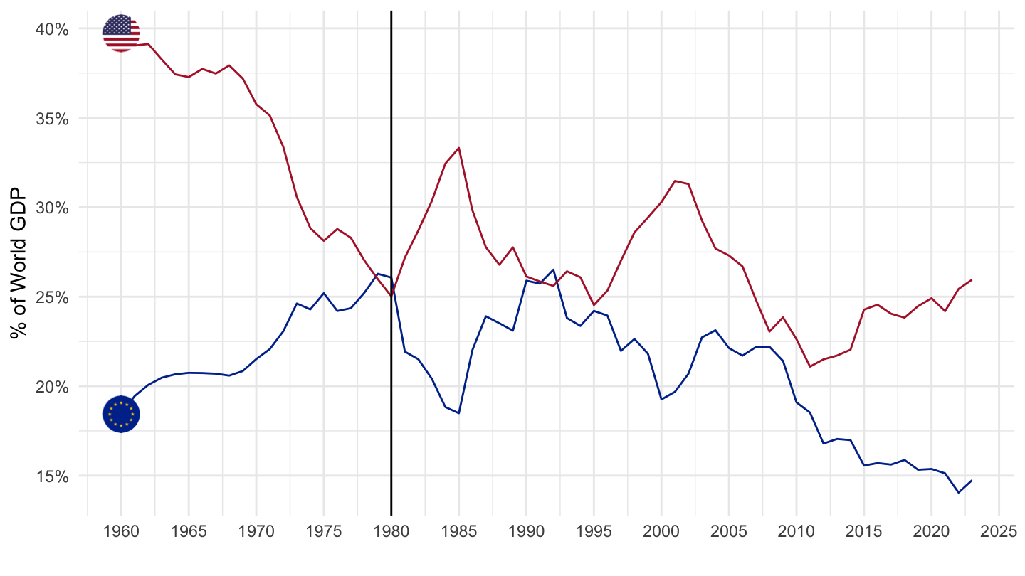
Eurozone, United States
All
Code
NY.GDP.MKTP.CD %>%
  right_join(iso2c, by = "iso2c") %>%
  filter(iso2c %in% c("1W", "XC", "US")) %>%
  group_by(year) %>%
  mutate(value = value/value[iso2c == "1W"]) %>%
  year_to_date %>%
  filter(!(iso2c == "1W")) %>%
  mutate(Iso2c = ifelse(iso2c == "XC", "Europe", Iso2c)) %>%
  left_join(colors, by = c("Iso2c" = "country")) %>%
  mutate(color = ifelse(iso2c == "US", color2, color)) %>%
  ggplot(.) + theme_minimal() + scale_color_identity() +
  geom_line(aes(x = date, y = value, color = color)) +
  add_flags +
  theme(legend.title = element_blank(),
        legend.position = c(0.85, 0.85)) +
  scale_x_date(breaks = seq(1950, 2100, 5) %>% paste0("-01-01") %>% as.Date,
               labels = date_format("%Y")) +
  scale_y_continuous(breaks = 0.01*seq(0, 70, 5),
                     labels = scales::percent_format(accuracy = 1)) +
  xlab("") + ylab("% of World GDP")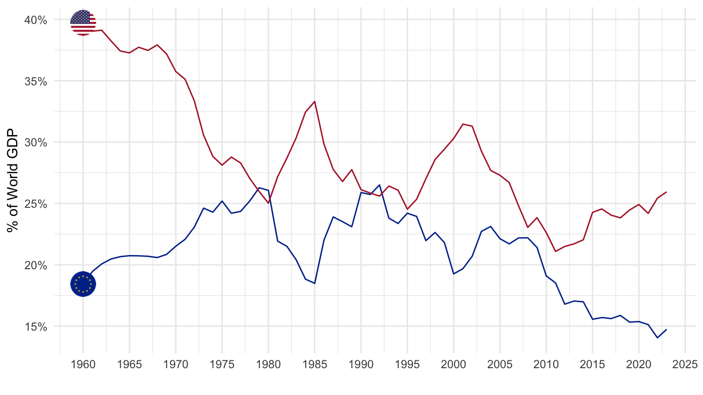
1990-
Code
NY.GDP.MKTP.CD %>%
  right_join(iso2c, by = "iso2c") %>%
  filter(iso2c %in% c("1W", "XC", "US")) %>%
  group_by(year) %>%
  mutate(value = value/value[iso2c == "1W"]) %>%
  year_to_date %>%
  filter(!(iso2c == "1W"),
         date >= as.Date("1990-01-01")) %>%
  mutate(Iso2c = ifelse(iso2c == "XC", "Europe", Iso2c)) %>%
  left_join(colors, by = c("Iso2c" = "country")) %>%
  mutate(color = ifelse(iso2c == "US", color2, color)) %>%
  ggplot(.) + theme_minimal() + scale_color_identity() +
  geom_line(aes(x = date, y = value, color = color)) +
  add_flags +
  theme(legend.title = element_blank(),
        legend.position = c(0.85, 0.85)) +
  scale_x_date(breaks = seq(1950, 2100, 5) %>% paste0("-01-01") %>% as.Date,
               labels = date_format("%Y")) +
  scale_y_continuous(breaks = 0.01*seq(0, 70, 5),
                     labels = scales::percent_format(accuracy = 1),
                     limits = 0.01*c(0, 35)) +
  xlab("") + ylab("% of World GDP")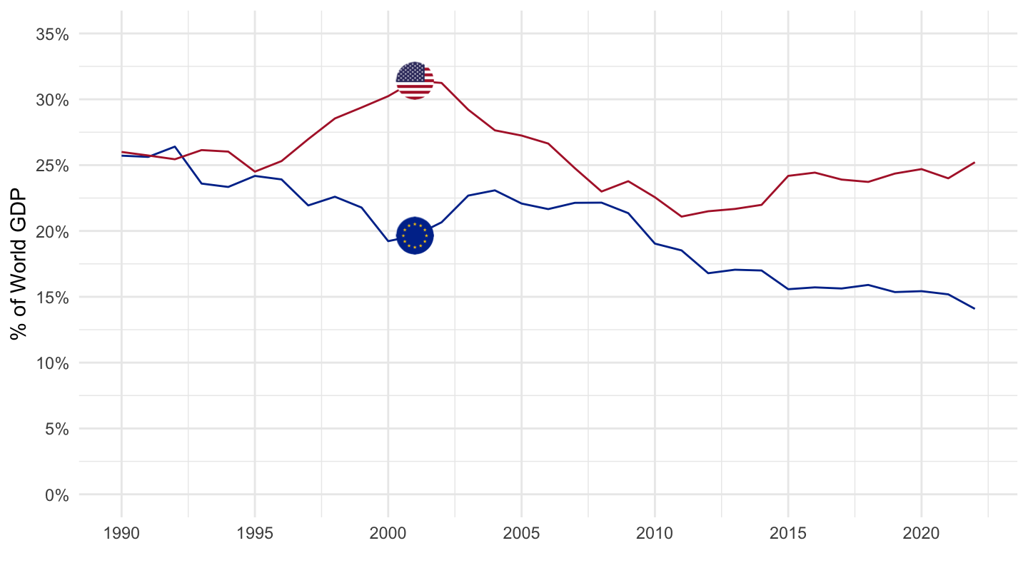
2005-
Code
NY.GDP.MKTP.CD %>%
  right_join(iso2c, by = "iso2c") %>%
  filter(iso2c %in% c("1W", "XC", "US")) %>%
  group_by(year) %>%
  mutate(value = value/value[iso2c == "1W"]) %>%
  year_to_date %>%
  filter(!(iso2c == "1W"),
         date >= as.Date("2005-01-01")) %>%
  mutate(Iso2c = ifelse(iso2c == "XC", "Europe", Iso2c)) %>%
  left_join(colors, by = c("Iso2c" = "country")) %>%
  mutate(color = ifelse(iso2c == "US", color2, color)) %>%
  ggplot(.) + theme_minimal() + scale_color_identity() + add_flags +
  geom_line(aes(x = date, y = value, color = color)) +
  scale_x_date(breaks = seq(1950, 2100, 1) %>% paste0("-01-01") %>% as.Date,
               labels = date_format("%Y")) +
  scale_y_continuous(breaks = 0.01*seq(0, 70, 5),
                     labels = scales::percent_format(accuracy = 1),
                     limits = 0.01*c(0, 35)) +
  xlab("") + ylab("% of World GDP")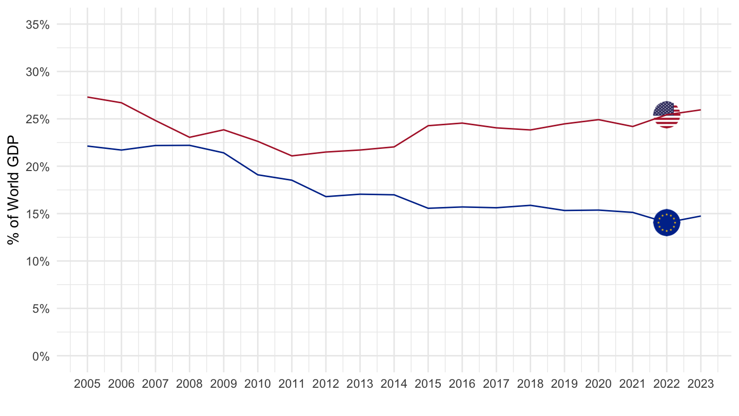
Germany, Japan, United Kingdom
Code
NY.GDP.MKTP.CD %>%
  right_join(iso2c, by = "iso2c") %>%
  filter(iso2c %in% c("1W", "JP", "DE", "GB")) %>%
  group_by(year) %>%
  mutate(value = value/value[iso2c == "1W"]) %>%
  year_to_date %>%
  filter(!(iso2c == "1W")) %>%
  left_join(colors, by = c("Iso2c" = "country")) %>%
  ggplot(.) + theme_minimal() + scale_color_identity() +
  geom_line(aes(x = date, y = value, color = color)) +
  add_flags +
  theme(legend.title = element_blank(),
        legend.position = c(0.85, 0.85)) +
  scale_x_date(breaks = seq(1950, 2100, 5) %>% paste0("-01-01") %>% as.Date,
               labels = date_format("%Y")) +
  scale_y_continuous(breaks = 0.01*seq(0, 70, 3),
                     labels = scales::percent_format(accuracy = 1),
                     limits = 0.01*c(0, 20)) +
  xlab("") + ylab("% of World GDP")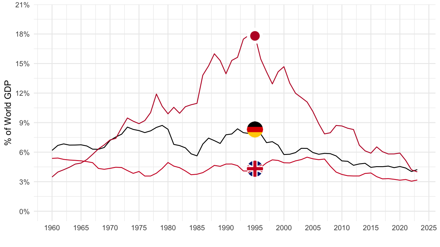
United Kingdom, France, Italy
Code
NY.GDP.MKTP.CD %>%
  right_join(iso2c, by = "iso2c") %>%
  filter(iso2c %in% c("1W", "GB", "FR", "IT")) %>%
  group_by(year) %>%
  mutate(value = value/value[iso2c == "1W"]) %>%
  year_to_date %>%
  filter(!(iso2c == "1W")) %>%
  left_join(colors, by = c("Iso2c" = "country")) %>%
  ggplot(.) + theme_minimal() + scale_color_identity() +
  geom_line(aes(x = date, y = value, color = color)) +
  add_flags +
  theme(legend.title = element_blank(),
        legend.position = c(0.85, 0.85)) +
  scale_x_date(breaks = seq(1950, 2100, 5) %>% paste0("-01-01") %>% as.Date,
               labels = date_format("%Y")) +
  scale_y_continuous(breaks = 0.01*seq(0, 70, 1),
                     labels = scales::percent_format(accuracy = 1),
                     limits = 0.01*c(0, 8)) +
  xlab("") + ylab("% of World GDP")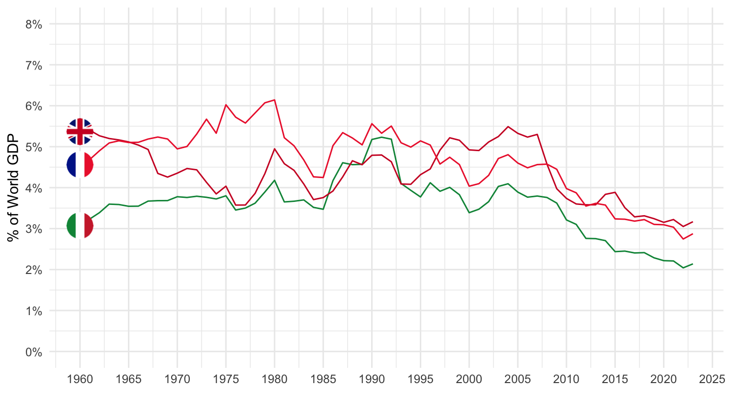
Brazil, Russia, India
Code
NY.GDP.MKTP.CD %>%
  right_join(iso2c, by = "iso2c") %>%
  filter(iso2c %in% c("1W", "BR", "RU", "IN")) %>%
  group_by(year) %>%
  mutate(value = value/value[iso2c == "1W"]) %>%
  year_to_date %>%
  filter(!(iso2c == "1W")) %>%
  mutate(Iso2c = ifelse(iso2c == "RU", "Russia", Iso2c)) %>%
  left_join(colors, by = c("Iso2c" = "country")) %>%
  ggplot(.) + theme_minimal() + scale_color_identity() +
  geom_line(aes(x = date, y = value, color = color)) +
  add_flags +
  theme(legend.title = element_blank(),
        legend.position = c(0.3, 0.85)) +
  scale_x_date(breaks = seq(1950, 2100, 5) %>% paste0("-01-01") %>% as.Date,
               labels = date_format("%Y")) +
  scale_y_continuous(breaks = 0.01*seq(0, 70, 1),
                     labels = scales::percent_format(accuracy = 1),
                     limits = 0.01*c(0, 5)) +
  xlab("") + ylab("% of World GDP")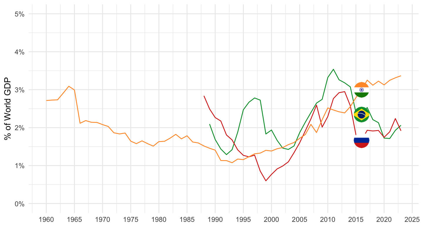
Euro Area vs. US
Base 100
Code
NY.GDP.MKTP.CD %>%
  left_join(iso2c, by = "iso2c") %>%
  year_to_date %>%
  filter(iso2c %in% c("XC", "US"),
         date >= as.Date("2008-01-01")) %>%
  group_by(iso2c) %>%
  arrange(date) %>%
  mutate(value = 100*value/value[1]) %>%
  mutate(Iso2c = ifelse(iso2c == "XC", "Europe", Iso2c)) %>%
  left_join(colors, by = c("Iso2c" = "country")) %>%
  mutate(color = ifelse(iso2c == "US", color2, color)) %>%
  ggplot(.) + theme_minimal() + scale_color_identity() +
  geom_line(aes(x = date, y = value, color = color)) +
  add_flags +
  scale_x_date(breaks = seq(1950, 2100, 2) %>% paste0("-01-01") %>% as.Date,
               labels = date_format("%Y")) +
  scale_y_log10(breaks = seq(70, 200, 5)) +
  xlab("") + ylab("PIB en $ (100 = 2008)")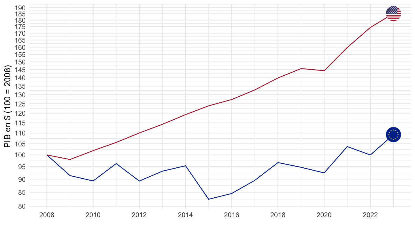
Avec dollars
Code
NY.GDP.MKTP.CD %>%
  left_join(iso2c, by = "iso2c") %>%
  year_to_date %>%
  filter(iso2c %in% c("XC", "US"),
         date >= as.Date("2008-01-01")) %>%
  group_by(iso2c) %>%
  arrange(date) %>%
  mutate(Iso2c = ifelse(iso2c == "XC", "Europe", Iso2c)) %>%
  left_join(colors, by = c("Iso2c" = "country")) %>%
  mutate(color = ifelse(iso2c == "US", color2, color)) %>%
  ungroup %>%
  mutate(dollar = value/10^9,
         value = 100*value/value[2]) %>%
  ggplot(.) + theme_minimal() + scale_color_identity() +
  geom_line(aes(x = date, y = value, color = color)) +
  add_flags +
  scale_x_date(breaks = seq(1950, 2100, 2) %>% paste0("-01-01") %>% as.Date,
               labels = date_format("%Y")) +
  scale_y_log10(breaks = seq(10, 200, 5)) +
  xlab("") + ylab("PIB en $ (100 = Zone Euro, 2008)") +
  geom_text_repel(data = . %>% filter(year(date) %in% seq(2008, 2022, 2)),
                                      aes(x = date, y = value, label = paste0("$", round(dollar, digits = -2), " Md")))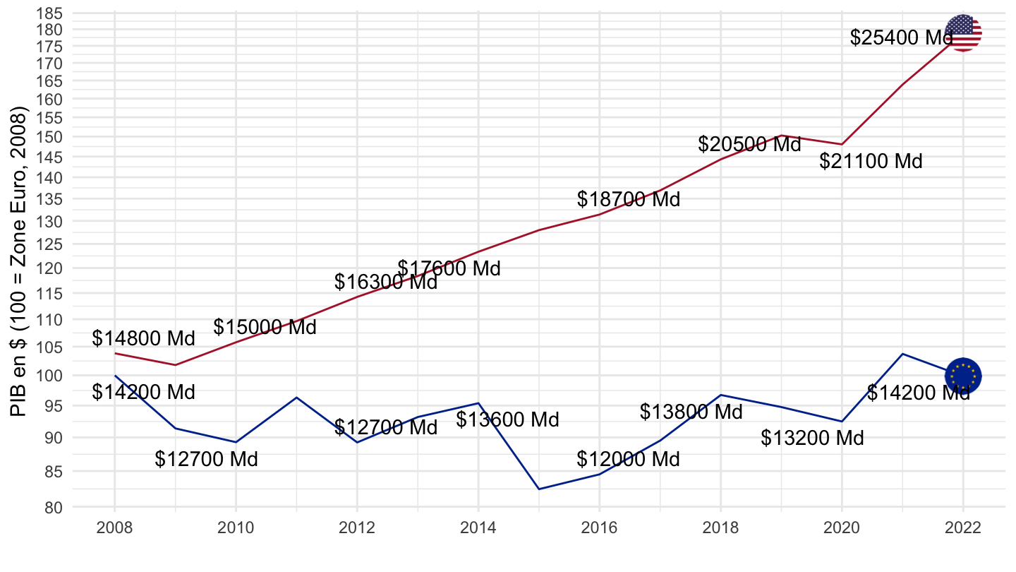
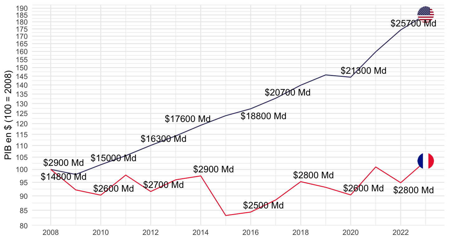
France vs. US
Avec dollars
Code
NY.GDP.MKTP.CD %>%
  left_join(iso2c, by = "iso2c") %>%
  year_to_date %>%
  filter(iso2c %in% c("FR", "US"),
         date >= as.Date("2008-01-01")) %>%
  group_by(iso2c) %>%
  arrange(date) %>%
  mutate(Iso2c = ifelse(iso2c == "FR", "France", Iso2c)) %>%
  left_join(colors, by = c("Iso2c" = "country")) %>%
  #mutate(color = ifelse(iso2c == "US", color2, color)) %>%
  #ungroup %>%
  mutate(dollar = value/10^9,
         value = 100*value/value[1]) %>%
  ggplot(.) + theme_minimal() + scale_color_identity() +
  geom_line(aes(x = date, y = value, color = color)) +
  add_flags +
  scale_x_date(breaks = seq(1950, 2100, 2) %>% paste0("-01-01") %>% as.Date,
               labels = date_format("%Y")) +
  scale_y_log10(breaks = seq(10, 200, 5)) +
  xlab("") + ylab("PIB en $ (100 = 2008)") +
  geom_text_repel(data = . %>% filter(year(date) %in% seq(2008, 2022, 2)),
                                      aes(x = date, y = value, label = paste0("$", round(dollar, digits = -2), " Md")))