Gross value added and income by A*10 industry breakdowns

Data - Eurostat

Author

Info

source	dataset	.html	.RData
eurostat	nama_10_a10	2024-09-15	2024-09-15

Data on macro

source	dataset	.html	.RData
eurostat	nama_10_a10	2024-09-15	2024-09-15
eurostat	nama_10_a10_e	2024-09-19	2024-09-18
eurostat	nama_10_gdp	2024-09-15	2024-09-15
eurostat	nama_10_lp_ulc	2024-09-15	2024-09-15
eurostat	namq_10_a10	2024-09-15	2024-09-18
eurostat	namq_10_a10_e	2024-09-15	2024-09-15
eurostat	namq_10_gdp	2024-09-04	2024-09-15
eurostat	namq_10_lp_ulc	2024-09-15	2024-09-15
eurostat	namq_10_pc	2024-08-21	2024-09-18
eurostat	nasa_10_nf_tr	2024-09-15	2024-09-15
eurostat	nasq_10_nf_tr	2024-09-02	2024-09-02
fred	gdp	2024-08-29	2024-09-18
oecd	QNA	2024-06-06	2024-06-30
oecd	SNA_TABLE1	2024-09-15	2024-06-30
oecd	SNA_TABLE14A	2024-09-15	2024-06-30
oecd	SNA_TABLE2	2024-07-01	2024-04-11
oecd	SNA_TABLE6A	2024-07-01	2024-06-30
wdi	NE.RSB.GNFS.ZS	2024-09-18	2024-09-18
wdi	NY.GDP.MKTP.CD	2024-09-18	2024-09-18
wdi	NY.GDP.MKTP.PP.CD	2024-09-18	2024-09-18
wdi	NY.GDP.PCAP.CD	2024-09-18	2024-09-18
wdi	NY.GDP.PCAP.KD	2024-09-18	2024-09-18
wdi	NY.GDP.PCAP.PP.CD	2024-09-18	2024-09-18
wdi	NY.GDP.PCAP.PP.KD	2024-09-18	2024-09-18

LAST_COMPILE

LAST_COMPILE
2024-09-19

Last

Code

nama_10_a10 %>%
  group_by(time) %>%
  summarise(Nobs = n()) %>%
  arrange(desc(time)) %>%
  head(1) %>%
  print_table_conditional()

time	Nobs
2023	22443

na_item

Code

nama_10_a10 %>%
  left_join(na_item, by = "na_item") %>%
  group_by(na_item, Na_item) %>%
  summarise(Nobs = n()) %>%
  arrange(-Nobs) %>%
  print_table_conditional()

na_item	Na_item	Nobs
B1G	Value added, gross	427884
D1	Compensation of employees	102334
D11	Wages and salaries	98990
D12	Employers' social contributions	98990

nace_r2

Code

nama_10_a10 %>%
  left_join(nace_r2, by = "nace_r2") %>%
  group_by(nace_r2, Nace_r2) %>%
  summarise(Nobs = n()) %>%
  arrange(-Nobs) %>%
  print_table_conditional()

nace_r2	Nace_r2	Nobs
TOTAL	Total - all NACE activities	61523
A	Agriculture, forestry and fishing	60657
B-E	Industry (except construction)	60657
C	Manufacturing	60657
F	Construction	60657
K	Financial and insurance activities	60657
O-Q	Public administration, defence, education, human health and social work activities	60657
R-U	Arts, entertainment and recreation; other service activities; activities of household and extra-territorial organizations and bodies	60657
G-I	Wholesale and retail trade, transport, accommodation and food service activities	60534
M_N	Professional, scientific and technical activities; administrative and support service activities	60534
L	Real estate activities	60530
J	Information and communication	60478

geo

Code

nama_10_a10 %>%
  left_join(geo, by = "geo") %>%
  group_by(geo, Geo) %>%
  summarise(Nobs = n()) %>%
  arrange(-Nobs) %>%
  mutate(Geo = ifelse(geo == "DE", "Germany", Geo)) %>%
  mutate(Flag = gsub(" ", "-", str_to_lower(Geo)),
         Flag = paste0('<img src="../../bib/flags/vsmall/', Flag, '.png" alt="Flag">')) %>%
  select(Flag, everything()) %>%
  {if (is_html_output()) datatable(., filter = 'top', rownames = F, escape = F) else .}

unit

Code

nama_10_a10 %>%
  left_join(unit, by = "unit") %>%
  group_by(unit, Unit) %>%
  summarise(Nobs = n()) %>%
  arrange(-Nobs) %>%
  print_table_conditional()

unit	Unit	Nobs
CP_MEUR	Current prices, million euro	60568
CP_MNAC	Current prices, million units of national currency	60568
PC_GDP	Percentage of gross domestic product (GDP)	60427
PC_TOT	Percentage of total	60427
PC_EU27_2020_MEUR_CP	Percentage of EU27 (from 2020) total (based on million euro), current prices	56625
CP_MPPS_EU27_2020	Current prices, million purchasing power standards (PPS, EU27 from 2020)	55462
PC_EU27_2020_MPPS_CP	Percentage of EU27 (from 2020) total (based on million purchasing power standards), current prices	55462
CLV10_MEUR	Chain linked volumes (2010), million euro	15406
CLV10_MNAC	Chain linked volumes (2010), million units of national currency	15406
CLV15_MEUR	Chain linked volumes (2015), million euro	15406
CLV15_MNAC	Chain linked volumes (2015), million units of national currency	15406
CLV_I10	Chain linked volumes, index 2010=100	15406
CLV_I15	Chain linked volumes, index 2015=100	15406
PD10_EUR	Price index (implicit deflator), 2010=100, euro	15386
PD10_NAC	Price index (implicit deflator), 2010=100, national currency	15386
PD15_EUR	Price index (implicit deflator), 2015=100, euro	15386
PD15_NAC	Price index (implicit deflator), 2015=100, national currency	15386
PYP_MNAC	Previous year prices, million units of national currency	15186
PYP_MEUR	Previous year prices, million euro	15174
CLV05_MEUR	Chain linked volumes (2005), million euro	14998
CLV05_MNAC	Chain linked volumes (2005), million units of national currency	14998
CLV_I05	Chain linked volumes, index 2005=100	14998
PD05_EUR	Price index (implicit deflator), 2005=100, euro	14978
PD05_NAC	Price index (implicit deflator), 2005=100, national currency	14978
CLV_PCH_PRE	Chain linked volumes, percentage change on previous period	14927
PD_PCH_PRE_NAC	Price index (implicit deflator), percentage change on previous period, national currency	14906
PD_PCH_PRE_EUR	Price index (implicit deflator), percentage change on previous period, euro	14894
CON_PPCH_PRE	Contribution to GDP growth, percentage point change on previous period	14642

Gross Domestic Product

2019, Table

Code

nama_10_a10 %>%
  filter(geo %in% c("FR", "DE", "IT"),
         # B1GQ: Gross domestic product at market prices
         na_item == "B1G",
         nace_r2 == "TOTAL",
         time == "2019") %>%
  left_join(geo, by = "geo") %>%
  select(-geo) %>%
  left_join(unit, by = "unit") %>%
  select_if(~ n_distinct(.) > 1) %>%
  spread(Geo, values) %>%
  print_table_conditional()

unit	Unit	France	Germany	Italy
CLV_I05	Chain linked volumes, index 2005=100	118.651	123.997	100.669
CLV_I10	Chain linked volumes, index 2010=100	112.791	116.516	101.734
CLV_I15	Chain linked volumes, index 2015=100	106.511	107.258	104.453
CLV_PCH_PRE	Chain linked volumes, percentage change on previous period	2.100	0.700	0.500
CLV05_MEUR	Chain linked volumes (2005), million euro	1874285.400	2597952.400	1355114.800
CLV05_MNAC	Chain linked volumes (2005), million units of national currency	1874285.400	2597952.400	1355114.800
CLV10_MEUR	Chain linked volumes (2010), million euro	2021882.100	2728763.100	1474565.100
CLV10_MNAC	Chain linked volumes (2010), million units of national currency	2021882.100	2728763.100	1474565.100
CLV15_MEUR	Chain linked volumes (2015), million euro	2087958.100	2951672.100	1554314.600
CLV15_MNAC	Chain linked volumes (2015), million units of national currency	2087958.100	2951672.100	1554314.600
CON_PPCH_PRE	Contribution to GDP growth, percentage point change on previous period	1.860	0.630	0.440
CP_MEUR	Current prices, million euro	2150690.000	3159273.000	1611368.500
CP_MNAC	Current prices, million units of national currency	2150690.000	3159273.000	1611368.500
CP_MPPS_EU27_2020	Current prices, million purchasing power standards (PPS, EU27 from 2020)	1980961.200	2862127.000	1618691.500
PC_EU27_2020_MEUR_CP	Percentage of EU27 (from 2020) total (based on million euro), current prices	17.100	25.100	12.800
PC_EU27_2020_MPPS_CP	Percentage of EU27 (from 2020) total (based on million purchasing power standards), current prices	15.800	22.800	12.900
PC_GDP	Percentage of gross domestic product (GDP)	88.400	89.400	89.700
PC_TOT	Percentage of total	100.000	100.000	100.000
PD_PCH_PRE_EUR	Price index (implicit deflator), percentage change on previous period, euro	1.200	2.300	0.900
PD_PCH_PRE_NAC	Price index (implicit deflator), percentage change on previous period, national currency	1.200	2.300	0.900
PD05_EUR	Price index (implicit deflator), 2005=100, euro	114.747	121.606	118.910
PD05_NAC	Price index (implicit deflator), 2005=100, national currency	114.747	121.606	118.910
PD10_EUR	Price index (implicit deflator), 2010=100, euro	106.371	115.777	109.278
PD10_NAC	Price index (implicit deflator), 2010=100, national currency	106.371	115.777	109.278
PD15_EUR	Price index (implicit deflator), 2015=100, euro	103.004	107.033	103.671
PD15_NAC	Price index (implicit deflator), 2015=100, national currency	103.004	107.033	103.671
PYP_MEUR	Previous year prices, million euro	2125823.000	3087923.000	1597350.900
PYP_MNAC	Previous year prices, million units of national currency	2125823.000	3087923.000	1597350.900

Euros

Code

nama_10_a10 %>%
  filter(geo %in% c("FR", "DE", "IT"),
         # B1GQ: Gross domestic product at market prices
         na_item == "B1G",
         nace_r2 == "TOTAL",
         unit == "CLV10_MEUR") %>%
  left_join(geo, by = "geo") %>%
  year_to_date %>%
  left_join(colors, by = c("Geo" = "country")) %>%
  mutate(values = values/1000) %>%
  ggplot + geom_line(aes(x = date, y = values, color = color)) +
  scale_color_identity() + theme_minimal()  + add_3flags + xlab("") + ylab("") +
  scale_x_date(breaks = as.Date(paste0(seq(1960, 2020, 5), "-01-01")),
               labels = date_format("%Y")) +
  theme(legend.position = c(0.3, 0.85),
        legend.title = element_blank()) +
  scale_y_log10(breaks = seq(0, 3000, 100),
                labels = dollar_format(suffix = " Bn€", prefix = "", accuracy = 1))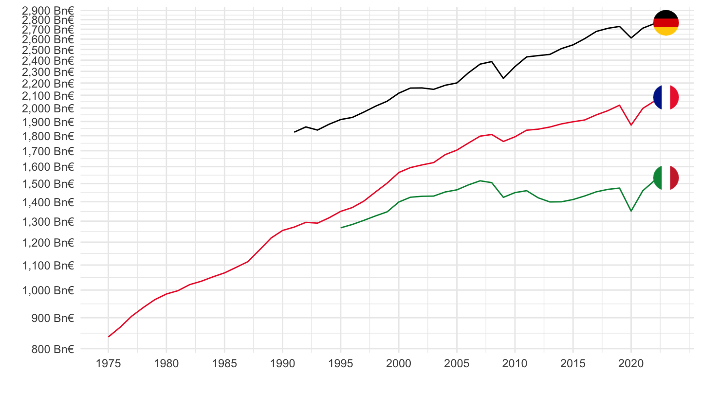

Manufacturing Compensation

Table

Code

nama_10_a10 %>%
  filter(geo %in% c("FR", "DE", "IT"),
         # B1GQ: Gross domestic product at market prices
         na_item == "D1",
         time == "2020",
         nace_r2 == "C") %>%
  left_join(unit, by = "unit") %>%
  left_join(geo, by = "geo") %>%
  select(-geo) %>%
  select_if(~ n_distinct(.) > 1) %>%
  mutate(Geo = gsub(" ", "-", str_to_lower(Geo)),
         Geo = paste0('<img src="../../bib/flags/vsmall/', Geo, '.png" alt="Flag">')) %>%
  spread(Geo, values) %>%
  {if (is_html_output()) datatable(., filter = 'top', rownames = F, escape = F) else .}

Nominal

Code

nama_10_a10 %>%
  filter(geo %in% c("FR", "DE", "IT"),
         # B1GQ: Gross domestic product at market prices
         na_item == "D1",
         nace_r2 == "C",
         unit == "CP_MEUR") %>%
  left_join(geo, by = "geo") %>%
  year_to_date %>%
  left_join(colors, by = c("Geo" = "country")) %>%
  mutate(values = values/1000) %>%
  ggplot + geom_line(aes(x = date, y = values, color = color)) +
  scale_color_identity() + theme_minimal()  + add_3flags + xlab("") + ylab("") +
  scale_x_date(breaks = as.Date(paste0(seq(1960, 2020, 5), "-01-01")),
               labels = date_format("%Y")) +
  theme(legend.position = c(0.3, 0.85),
        legend.title = element_blank()) +
  scale_y_log10(breaks = seq(0, 3000, 100),
                labels = dollar_format(suffix = " Bn€", prefix = "", accuracy = 1))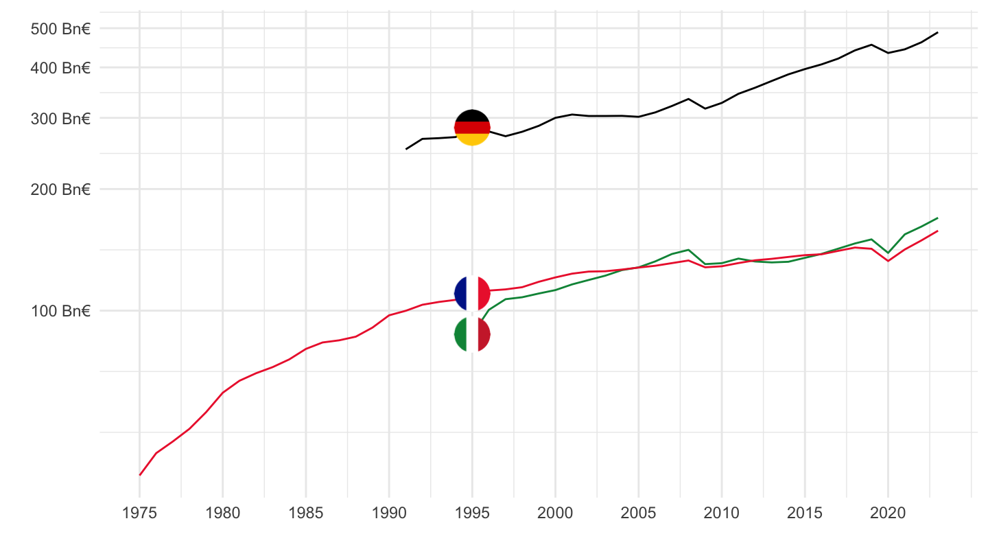

Manufacturing Value Added

Table

Code

nama_10_a10 %>%
  filter(geo %in% c("FR", "DE", "IT"),
         # B1GQ: Gross domestic product at market prices
         na_item == "B1G",
         time == "2020",
         nace_r2 == "C") %>%
  left_join(unit, by = "unit") %>%
  left_join(geo, by = "geo") %>%
  select(-geo) %>%
  select_if(~ n_distinct(.) > 1) %>%
  mutate(Geo = gsub(" ", "-", str_to_lower(Geo)),
         Geo = paste0('<img src="../../bib/flags/vsmall/', Geo, '.png" alt="Flag">')) %>%
  spread(Geo, values) %>%
  {if (is_html_output()) datatable(., filter = 'top', rownames = F, escape = F) else .}

Real

Code

nama_10_a10 %>%
  filter(geo %in% c("FR", "DE", "IT"),
         # B1GQ: Gross domestic product at market prices
         na_item == "B1G",
         nace_r2 == "C",
         unit == "CLV10_MEUR") %>%
  left_join(geo, by = "geo") %>%
  year_to_date %>%
  left_join(colors, by = c("Geo" = "country")) %>%
  mutate(values = values/1000) %>%
  ggplot + geom_line(aes(x = date, y = values, color = color)) +
  scale_color_identity() + theme_minimal()  + add_3flags + xlab("") + ylab("") +
  scale_x_date(breaks = as.Date(paste0(seq(1960, 2020, 5), "-01-01")),
               labels = date_format("%Y")) +
  theme(legend.position = c(0.3, 0.85),
        legend.title = element_blank()) +
  scale_y_log10(breaks = seq(0, 3000, 100),
                labels = dollar_format(suffix = " Bn€", prefix = "", accuracy = 1))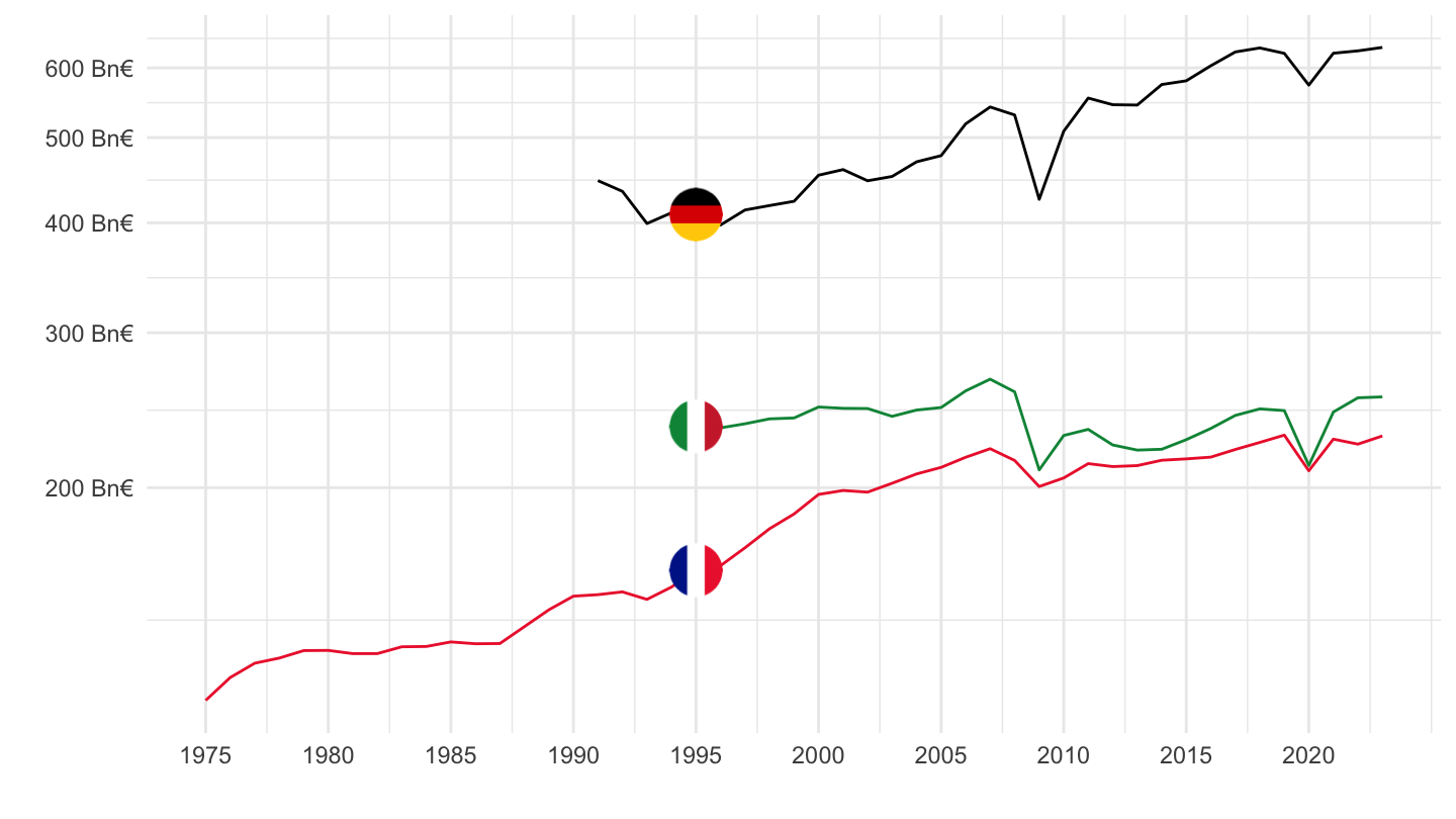

Nominal

Code

nama_10_a10 %>%
  filter(geo %in% c("FR", "DE", "IT"),
         # B1GQ: Gross domestic product at market prices
         na_item == "B1G",
         nace_r2 == "C",
         unit == "CP_MNAC") %>%
  left_join(geo, by = "geo") %>%
  year_to_date %>%
  left_join(colors, by = c("Geo" = "country")) %>%
  mutate(values = values/1000) %>%
  ggplot + geom_line(aes(x = date, y = values, color = color)) +
  scale_color_identity() + theme_minimal()  + add_3flags + xlab("") + ylab("") +
  scale_x_date(breaks = as.Date(paste0(seq(1960, 2020, 5), "-01-01")),
               labels = date_format("%Y")) +
  theme(legend.position = c(0.3, 0.85),
        legend.title = element_blank()) +
  scale_y_log10(breaks = seq(0, 3000, 100),
                labels = dollar_format(suffix = " Bn€", prefix = "", accuracy = 1))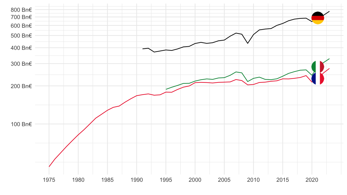

Manufacturing Value Added (% of GDP)

2019 France, Germany, Italy

Code

nama_10_a10 %>%
  filter(geo %in% c("FR", "DE", "IT"),
         unit == "CP_MNAC",
         na_item == "B1G",
         time == "2019") %>%
  left_join(nace_r2, by = "nace_r2") %>%
  select(geo, nace_r2, Nace_r2, values) %>%
  group_by(geo) %>%
  mutate(values = round(100*values /values[nace_r2 =="TOTAL"], 1)) %>%
  spread(geo, values) %>%
  filter(nace_r2 != "TOTAL") %>%
  arrange(-FR) %>%
  {if (is_html_output()) datatable(., filter = 'top', rownames = F) else .}

France: 2019, 1999, 1979

Code

nama_10_a10 %>%
  filter(geo %in% c("FR"),
         unit == "CP_MNAC",
         na_item == "B1G",
         time %in% c("2019",  "1999", 1979)) %>%
  left_join(nace_r2, by = "nace_r2") %>%
  select(time, nace_r2, Nace_r2, values) %>%
  group_by(time) %>%
  mutate(values = round(100*values /values[nace_r2 =="TOTAL"], 1)) %>%
  spread(time, values) %>%
  filter(nace_r2 != "TOTAL") %>%
  arrange(-`2019`) %>%
  {if (is_html_output()) datatable(., filter = 'top', rownames = F) else .}

France, Germany, United Kingdom

Code

nama_10_a10 %>%
  filter(na_item == "B1G",
         nace_r2 %in% c("C", "TOTAL"),
         geo %in% c("FR", "DE", "UK"),
         unit == "CP_MNAC") %>%
  year_to_date() %>%
  left_join(geo, by = "geo") %>%
  select(geo,  Geo, nace_r2, date, values) %>%
  spread(nace_r2, values) %>%
  mutate(values = `C`/TOTAL) %>%
  left_join(colors, by = c("Geo" = "country")) %>%
  ggplot(.) + geom_line(aes(x = date, y =values, color = color)) + 
  theme_minimal() + xlab("") + ylab("Manufacturing Value added (% of GDP)") +
  scale_color_identity() +
  scale_x_date(breaks = seq(1960, 2025, 5) %>% paste0("-01-01") %>% as.Date,
               labels = date_format("%Y")) +
  add_3flags +
  theme(legend.position = "none") +
  scale_y_continuous(breaks = 0.01*seq(-500, 200, 1),
                     labels = percent_format(accuracy = 1))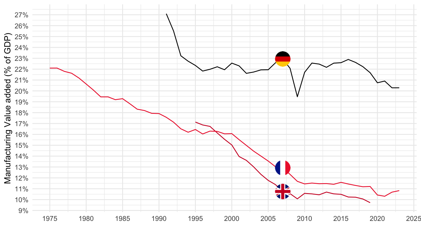

France, Germany, Greece, Italy, Portugal, Spain

All

Code

nama_10_a10 %>%
  filter(na_item == "B1G",
         nace_r2 %in% c("C", "TOTAL"),
         geo %in% c("FR", "DE", "EL", "ES", "IT", "PT"),
         unit == "CP_MNAC") %>%
  year_to_date() %>%
  filter(date >= as.Date("1995-01-01")) %>%
  left_join(geo, by = "geo") %>%
  select(geo,  Geo, nace_r2, date, values) %>%
  spread(nace_r2, values) %>%
  left_join(colors, by = c("Geo" = "country")) %>%
  mutate(values = C/TOTAL) %>%
  ggplot(.) + geom_line(aes(x = date, y = values, color = color)) + 
  theme_minimal() + xlab("") + ylab("Manufacturing Value added (% of GDP)") +
  scale_color_identity() +
  scale_x_date(breaks = seq(1960, 2100, 2) %>% paste0("-01-01") %>% as.Date,
               labels = date_format("%Y")) +
  add_6flags +
  theme(legend.position = "none") +
  scale_y_continuous(breaks = 0.01*seq(-500, 200, 1),
                     labels = percent_format(accuracy = 1))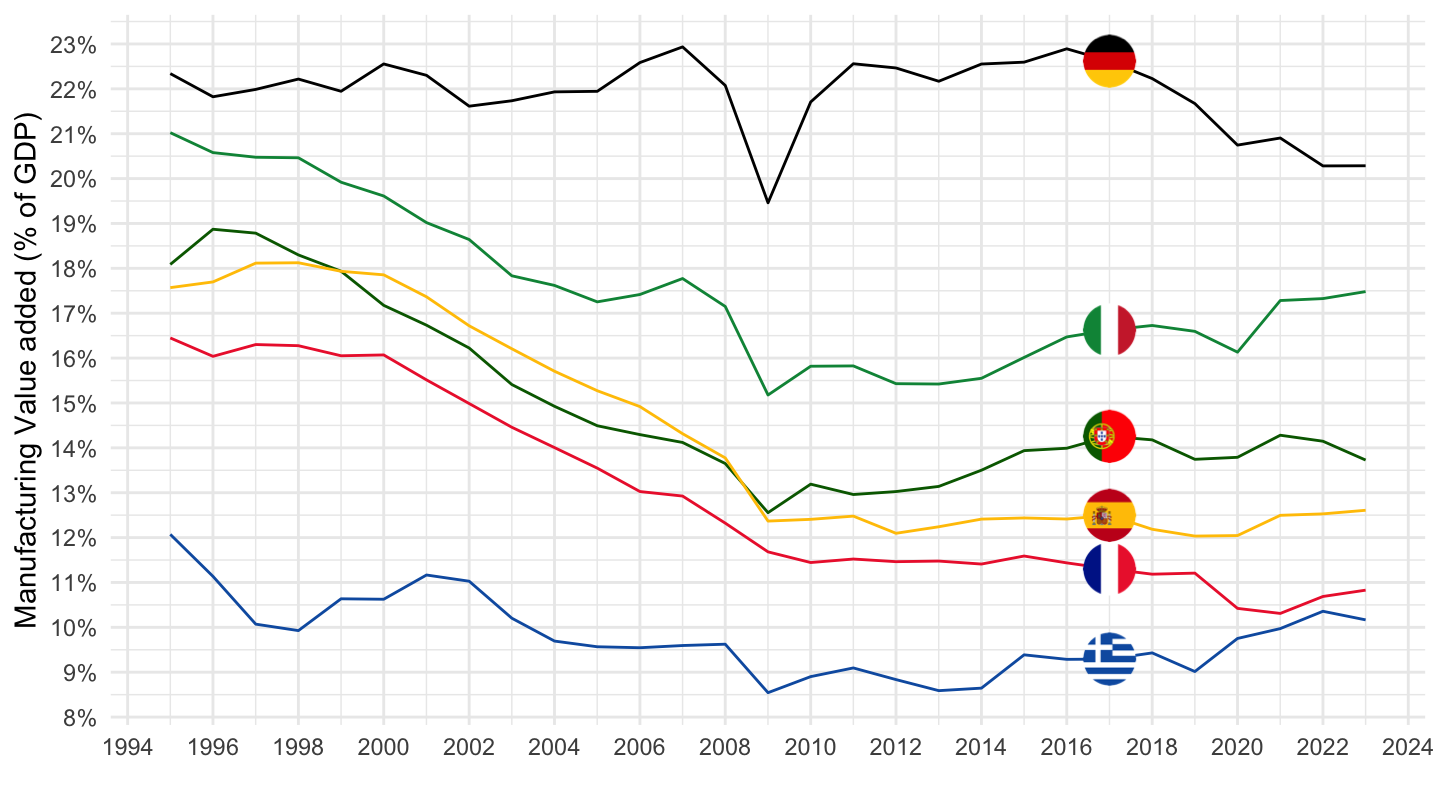

1995-

Code

nama_10_a10 %>%
  filter(na_item == "B1G",
         nace_r2 %in% c("C", "TOTAL"),
         geo %in% c("FR", "DE", "EL", "ES", "IT", "PT"),
         unit == "CP_MNAC") %>%
  year_to_date() %>%
  filter(date >= as.Date("1995-01-01")) %>%
  left_join(geo, by = "geo") %>%
  select(geo,  Geo, nace_r2, date, values) %>%
  spread(nace_r2, values) %>%
  left_join(colors, by = c("Geo" = "country")) %>%
  mutate(values = C/TOTAL) %>%
  ggplot(.) + geom_line(aes(x = date, y = values, color = color)) + 
  theme_minimal() + xlab("") + ylab("Manufacturing Value added (% of GDP)") +
  scale_color_identity() +
  scale_x_date(breaks = seq(1960, 2100, 5) %>% paste0("-01-01") %>% as.Date,
               labels = date_format("%Y")) +
  add_6flags +
  theme(legend.position = "none") +
  scale_y_continuous(breaks = 0.01*seq(-500, 200, 1),
                     labels = percent_format(accuracy = 1))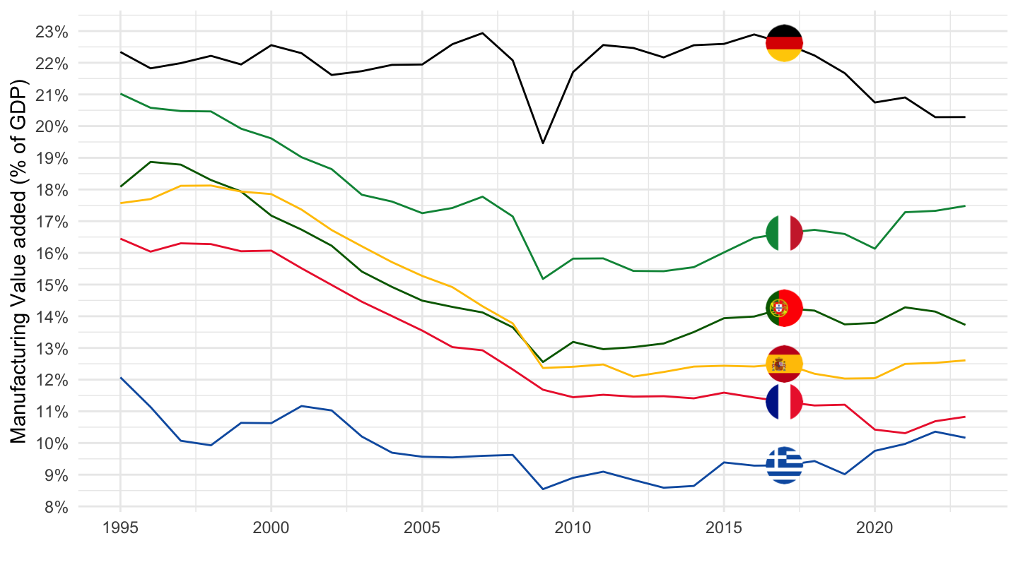

France, Luxembourg, Cyprus

1995-

Code

nama_10_a10 %>%
  filter(na_item == "B1G",
         nace_r2 %in% c("C", "TOTAL"),
         geo %in% c("FR", "ME", "LU", "CY", "MT", "EL"),
         unit == "CP_MNAC") %>%
  year_to_date() %>%
  filter(date >= as.Date("1995-01-01")) %>%
  left_join(geo, by = "geo") %>%
  select(geo,  Geo, nace_r2, date, values) %>%
  spread(nace_r2, values) %>%
  left_join(colors, by = c("Geo" = "country")) %>%
  mutate(values = C/TOTAL) %>%
  ggplot(.) + geom_line(aes(x = date, y = values, color = color)) + 
  theme_minimal() + xlab("") + ylab("Manufacturing Value added (% of GDP)") +
  scale_color_identity() +
  scale_x_date(breaks = seq(1960, 2100, 5) %>% paste0("-01-01") %>% as.Date,
               labels = date_format("%Y")) +
  add_6flags +
  theme(legend.position = "none") +
  scale_y_continuous(breaks = 0.01*seq(-500, 200, 1),
                     labels = percent_format(accuracy = 1))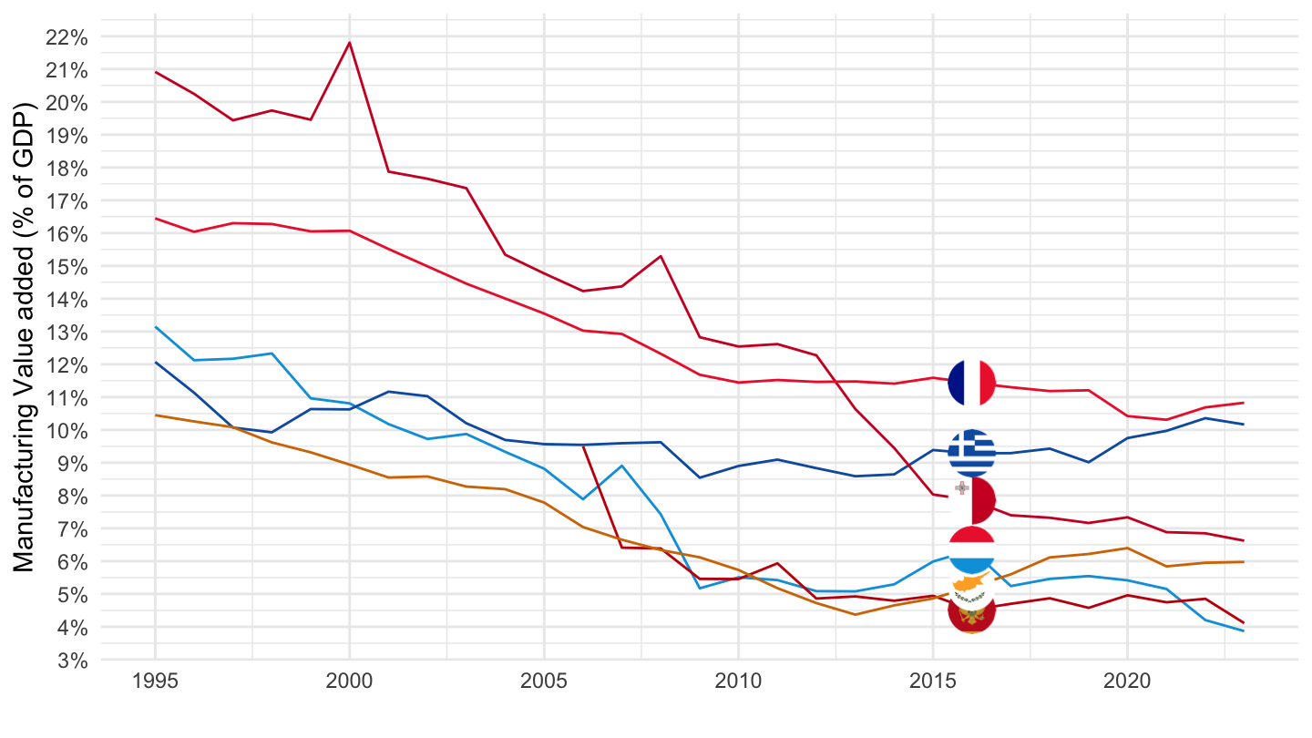

France, Italie, Allemagne, EA20

1995-

Code

load_data("eurostat/geo.RData")
nama_10_a10 %>%
  filter(na_item == "B1G",
         nace_r2 %in% c("C", "TOTAL"),
         geo %in% c("FR", "EA20", "IT", "DE"),
         unit == "CP_MNAC") %>%
  year_to_date() %>%
  filter(date >= as.Date("1995-01-01")) %>%
  left_join(geo, by = "geo") %>%
  mutate(Geo = ifelse(geo == "EA20", "Europe", Geo)) %>%
  select(geo,  Geo, nace_r2, date, values) %>%
  spread(nace_r2, values) %>%
  left_join(colors, by = c("Geo" = "country")) %>%
  mutate(values = C/TOTAL) %>%
  ggplot(.) + geom_line(aes(x = date, y = values, color = color)) + 
  theme_minimal() + xlab("") + ylab("Manufacturing Value added (% of GDP)") +
  scale_color_identity() +
  scale_x_date(breaks = seq(1960, 2100, 5) %>% paste0("-01-01") %>% as.Date,
               labels = date_format("%Y")) +
  add_4flags +
  theme(legend.position = "none") +
  scale_y_continuous(breaks = 0.01*seq(-500, 200, 1),
                     labels = percent_format(accuracy = 1))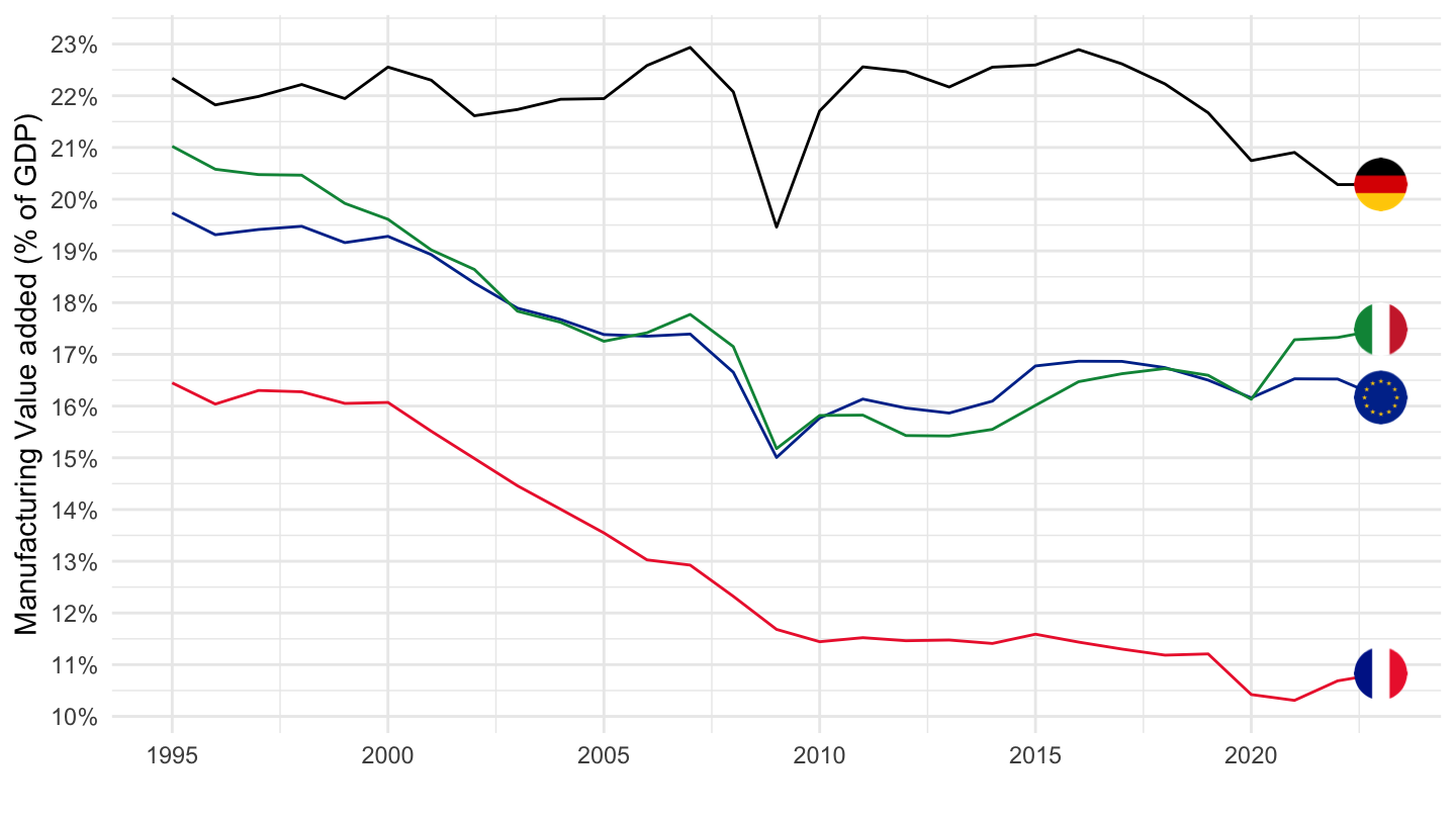

France, Greece, EA20

1995-

Code

nama_10_a10 %>%
  filter(na_item == "B1G",
         nace_r2 %in% c("C", "TOTAL"),
         geo %in% c("FR", "EA20", "EL"),
         unit == "CP_MNAC") %>%
  year_to_date() %>%
  filter(date >= as.Date("1995-01-01")) %>%
  left_join(geo, by = "geo") %>%
  mutate(Geo = ifelse(geo == "EA20", "Europe", Geo)) %>%
  select(geo,  Geo, nace_r2, date, values) %>%
  spread(nace_r2, values) %>%
  left_join(colors, by = c("Geo" = "country")) %>%
  mutate(values = C/TOTAL) %>%
  ggplot(.) + geom_line(aes(x = date, y = values, color = color)) + 
  theme_minimal() + xlab("") + ylab("Manufacturing Value added (% of GDP)") +
  scale_color_identity() +
  scale_x_date(breaks = seq(1960, 2100, 5) %>% paste0("-01-01") %>% as.Date,
               labels = date_format("%Y")) +
  add_3flags +
  theme(legend.position = "none") +
  scale_y_continuous(breaks = 0.01*seq(-500, 200, 1),
                     labels = percent_format(accuracy = 1))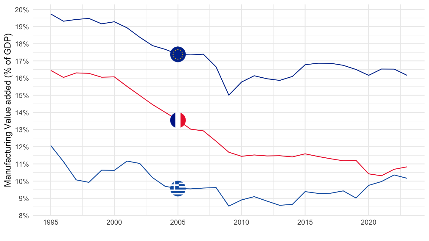

Greece, Portugal, Spain

Code

nama_10_a10 %>%
  filter(na_item == "B1G",
         nace_r2 %in% c("C", "TOTAL"),
         geo %in% c("EL", "PT", "ES"),
         unit == "CP_MNAC") %>%
  year_to_date() %>%
  left_join(geo, by = "geo") %>%
  select(Geo, nace_r2, date, values) %>%
  spread(nace_r2, values) %>%
  ggplot(.) + geom_line(aes(x = date, y = C/TOTAL, color = Geo)) + 
  theme_minimal() + xlab("") + ylab("Manufacturing Value added (% of GDP)") +
  scale_color_manual(values = c("#0D5EAF", "#006600", "#C60B1E")) +
  scale_x_date(breaks = seq(1960, 2025, 5) %>% paste0("-01-01") %>% as.Date,
               labels = date_format("%Y")) +
  geom_image(data = . %>%
               filter(date == as.Date("2016-01-01")) %>%
               mutate(date = as.Date("2016-01-01"),
                      image = paste0("../../icon/flag/", str_to_lower(Geo), ".png")),
             aes(x = date, y = C/TOTAL, image = image), asp = 1.5) +
  theme(legend.position = "none") +
  scale_y_continuous(breaks = 0.01*seq(-500, 200, 1),
                     labels = percent_format(accuracy = 1))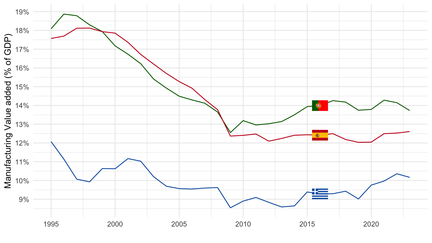

1995-2018

Code

nama_10_a10 %>%
  filter(na_item == "B1G",
         nace_r2 %in% c("C", "TOTAL"),
         geo %in% c("EA", "FR", "DE", "IT", "ES", "NL", "AT", "FI"),
         unit == "CP_MNAC") %>%
  year_to_date() %>%
  filter(date >= as.Date("1995-01-01"),
         date <= as.Date("2019-01-01")) %>%
  left_join(geo, by = "geo") %>%
  select(geo, Geo, nace_r2, date, values) %>%
  spread(nace_r2, values) %>%
  mutate(values = C/TOTAL) %>%
  group_by(date) %>%
  mutate(values = values /values[geo == "EA"]) %>%
  filter(geo != "EA") %>%
  group_by(geo) %>%
  mutate(values = 100*values / values[date == as.Date("1995-01-01")]) %>%
  left_join(colors, by = c("Geo" = "country")) %>%
  mutate(color = ifelse(geo == "FR", color2, color)) %>%
  ggplot(.) + geom_line(aes(x = date, y = values, color = color)) + 
  theme_minimal() + xlab("") + ylab("Valeur ajoutée manuf. par rapport à la Zone €") +
  scale_color_identity() + add_7flags +
  theme(legend.position = "none") +
  scale_x_date(breaks = seq(1995, 2025, 5) %>% paste0("-01-01") %>% as.Date,
               labels = date_format("%Y")) +
  scale_y_continuous(breaks = seq(0, 200, 5)) +
  theme(legend.position = "none") +
  geom_hline(yintercept = 100, linetype = "dashed")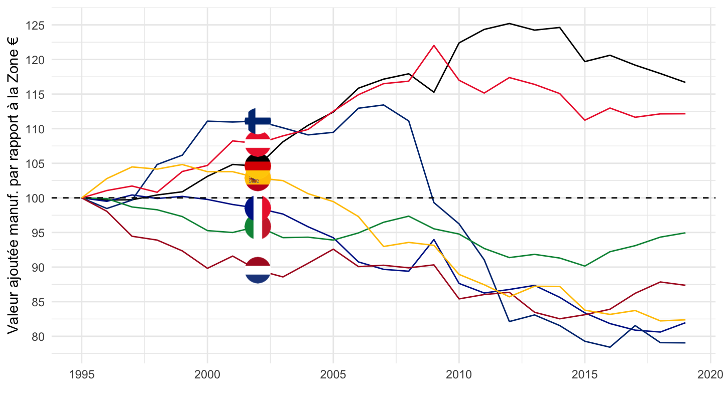

1995-

Code

nama_10_a10 %>%
  filter(na_item == "B1G",
         nace_r2 %in% c("C", "TOTAL"),
         geo %in% c("EA", "FR", "DE", "IT", "ES", "NL", "AT", "PL", "CZ"),
         unit == "CP_MNAC") %>%
  year_to_date() %>%
  filter(date >= as.Date("1995-01-01"),
         date <= as.Date("2019-01-01")) %>%
  left_join(geo, by = "geo") %>%
  select(geo, Geo, nace_r2, date, values) %>%
  spread(nace_r2, values) %>%
  mutate(values = C/TOTAL) %>%
  group_by(date) %>%
  mutate(values = values /values[geo == "EA"]) %>%
  filter(geo != "EA") %>%
  group_by(geo) %>%
  mutate(values = 100*values / values[date == as.Date("1995-01-01")]) %>%
  left_join(colors, by = c("Geo" = "country")) %>%
  mutate(color = ifelse(geo == "FR", color2, color)) %>%
  ggplot(.) + geom_line(aes(x = date, y = values, color = color)) + 
  theme_minimal() + xlab("") + ylab("Valeur ajoutée manuf. par rapport à la Zone €") +
  scale_color_identity() +
  add_8flags +
  theme(legend.position = "none") +
  scale_x_date(breaks = seq(1995, 2025, 5) %>% paste0("-01-01") %>% as.Date,
               labels = date_format("%Y")) +
  scale_y_log10(breaks = seq(0, 200, 5)) +
  theme(legend.position = "none") +
  geom_hline(yintercept = 100, linetype = "dashed")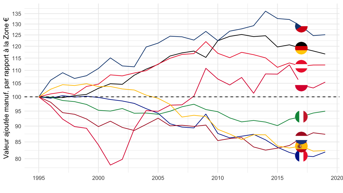

2000-2018

Code

nama_10_a10 %>%
  filter(na_item == "B1G",
         nace_r2 %in% c("C", "TOTAL"),
         geo %in% c("EA", "FR", "DE", "IT", "ES", "NL", "AT", "FI"),
         unit == "CP_MNAC") %>%
  year_to_date() %>%
  filter(date >= as.Date("2000-01-01"),
         date <= as.Date("2019-01-01")) %>%
  left_join(geo, by = "geo") %>%
  select(geo, Geo, nace_r2, date, values) %>%
  spread(nace_r2, values) %>%
  mutate(values = C/TOTAL) %>%
  group_by(date) %>%
  mutate(values = values /values[geo == "EA"]) %>%
  filter(geo != "EA") %>%
  group_by(geo) %>%
  mutate(values = 100*values / values[date == as.Date("2000-01-01")]) %>%
  left_join(colors, by = c("Geo" = "country")) %>%
  mutate(color = ifelse(geo == "FR", color2, color)) %>%
  ggplot(.) + geom_line(aes(x = date, y = values, color = color)) + 
  theme_minimal() + xlab("") + ylab("Valeur ajoutée manuf. par rapport à la Zone €") +
  scale_color_identity() + add_7flags +
  scale_x_date(breaks = seq(1960, 2020, 1) %>% paste0("-01-01") %>% as.Date,
               labels = date_format("%Y")) +
  scale_y_continuous(breaks = seq(0, 200, 5)) +
  theme(legend.position = "none") +
  geom_hline(yintercept = 100, linetype = "dashed")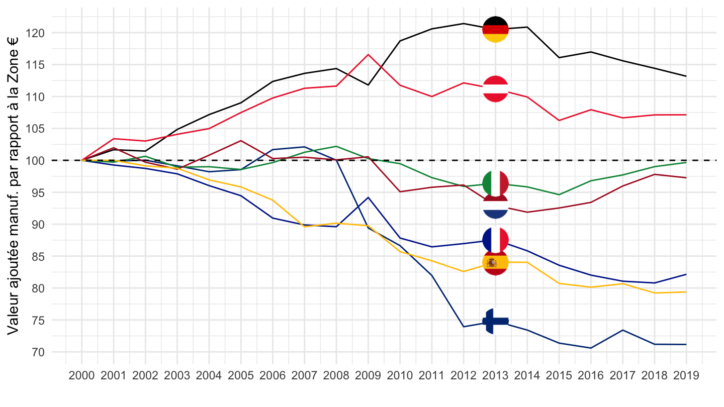

Industry Value Added (% of GDP)

2019 France, Germany, Italy

Code

nama_10_a10 %>%
  filter(geo %in% c("FR", "DE", "IT"),
         unit == "CP_MNAC",
         na_item == "B1G",
         time == "2019") %>%
  left_join(nace_r2, by = "nace_r2") %>%
  select(geo, nace_r2, Nace_r2, values) %>%
  group_by(geo) %>%
  mutate(values = round(100*values /values[nace_r2 =="TOTAL"], 1)) %>%
  spread(geo, values) %>%
  filter(nace_r2 != "TOTAL") %>%
  arrange(-FR) %>%
  {if (is_html_output()) datatable(., filter = 'top', rownames = F) else .}

France: 2019, 1999, 1979

Code

nama_10_a10 %>%
  filter(geo %in% c("FR"),
         unit == "CP_MNAC",
         na_item == "B1G",
         time %in% c("2019",  "1999", 1979)) %>%
  left_join(nace_r2, by = "nace_r2") %>%
  select(time, nace_r2, Nace_r2, values) %>%
  group_by(time) %>%
  mutate(values = round(100*values /values[nace_r2 =="TOTAL"], 1)) %>%
  spread(time, values) %>%
  filter(nace_r2 != "TOTAL") %>%
  arrange(-`2019`) %>%
  {if (is_html_output()) datatable(., filter = 'top', rownames = F) else .}

France, Germany, United Kingdom

Code

nama_10_a10 %>%
  filter(na_item == "B1G",
         nace_r2 %in% c("B-E", "TOTAL"),
         geo %in% c("FR", "DE", "UK"),
         unit == "CP_MNAC") %>%
  year_to_date() %>%
  left_join(geo, by = "geo") %>%
  select(geo,  Geo, nace_r2, date, values) %>%
  spread(nace_r2, values) %>%
  mutate(values = `B-E`/TOTAL) %>%
  left_join(colors, by = c("Geo" = "country")) %>%
  ggplot(.) + geom_line(aes(x = date, y =values, color = color)) + 
  theme_minimal() + xlab("") + ylab("Industry Value added (% of GDP)") +
  scale_color_identity() +
  scale_x_date(breaks = seq(1960, 2025, 5) %>% paste0("-01-01") %>% as.Date,
               labels = date_format("%Y")) +
  add_3flags +
  theme(legend.position = "none") +
  scale_y_continuous(breaks = 0.01*seq(-500, 200, 1),
                     labels = percent_format(accuracy = 1))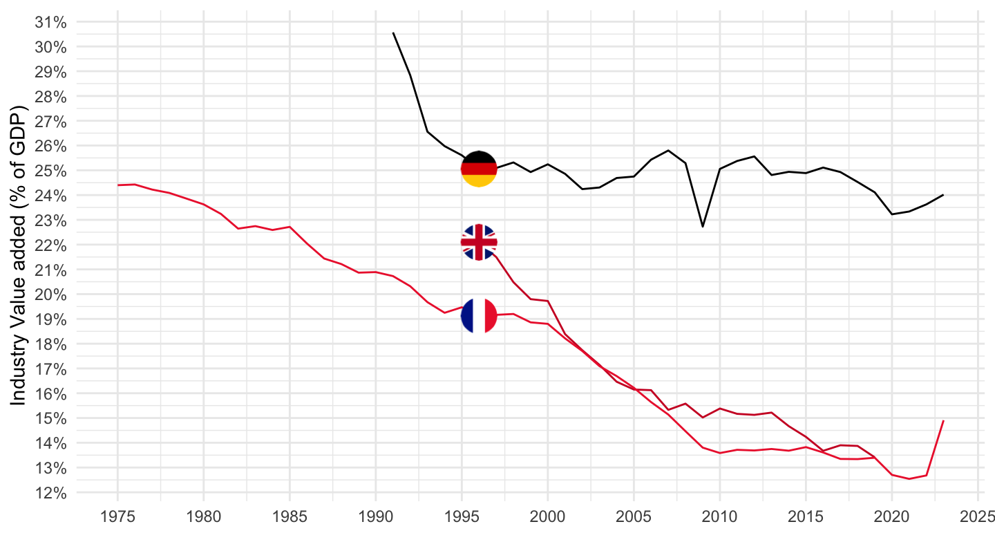

France, Greece, EA20

1995-

Code

nama_10_a10 %>%
  filter(na_item == "B1G",
         nace_r2 %in% c("B-E", "TOTAL"),
         geo %in% c("FR", "EA20", "EL"),
         unit == "CP_MNAC") %>%
  year_to_date() %>%
  filter(date >= as.Date("1995-01-01")) %>%
  left_join(geo, by = "geo") %>%
  mutate(Geo = ifelse(geo == "EA20", "Europe", Geo)) %>%
  select(geo,  Geo, nace_r2, date, values) %>%
  spread(nace_r2, values) %>%
  left_join(colors, by = c("Geo" = "country")) %>%
  mutate(values = `B-E`/TOTAL) %>%
  ggplot(.) + geom_line(aes(x = date, y = values, color = color)) + 
  theme_minimal() + xlab("") + ylab("Industry Value added (% of GDP)") +
  scale_color_identity() +
  scale_x_date(breaks = seq(1960, 2100, 5) %>% paste0("-01-01") %>% as.Date,
               labels = date_format("%Y")) +
  add_3flags +
  theme(legend.position = "none") +
  scale_y_continuous(breaks = 0.01*seq(-500, 200, 1),
                     labels = percent_format(accuracy = 1))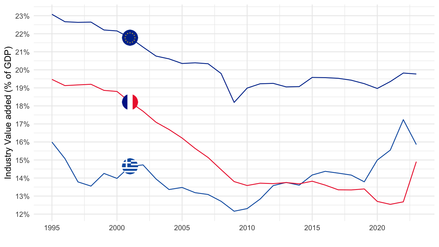

France, Greece, EA20

1995-

Code

nama_10_a10 %>%
  filter(na_item == "B1G",
         nace_r2 %in% c("B-E", "TOTAL"),
         geo %in% c("FR", "EA20", "EL", "DE", "IT"),
         unit == "CP_MNAC") %>%
  year_to_date() %>%
  filter(date >= as.Date("1995-01-01")) %>%
  left_join(geo, by = "geo") %>%
  mutate(Geo = ifelse(geo == "EA20", "Europe", Geo)) %>%
  select(geo,  Geo, nace_r2, date, values) %>%
  spread(nace_r2, values) %>%
  left_join(colors, by = c("Geo" = "country")) %>%
  mutate(values = `B-E`/TOTAL) %>%
  ggplot(.) + geom_line(aes(x = date, y = values, color = color)) + 
  theme_minimal() + xlab("") + ylab("Industry Value added (% of GDP)") +
  scale_color_identity() +
  scale_x_date(breaks = seq(1960, 2100, 5) %>% paste0("-01-01") %>% as.Date,
               labels = date_format("%Y")) +
  add_5flags +
  theme(legend.position = "none") +
  scale_y_continuous(breaks = 0.01*seq(-500, 200, 1),
                     labels = percent_format(accuracy = 1))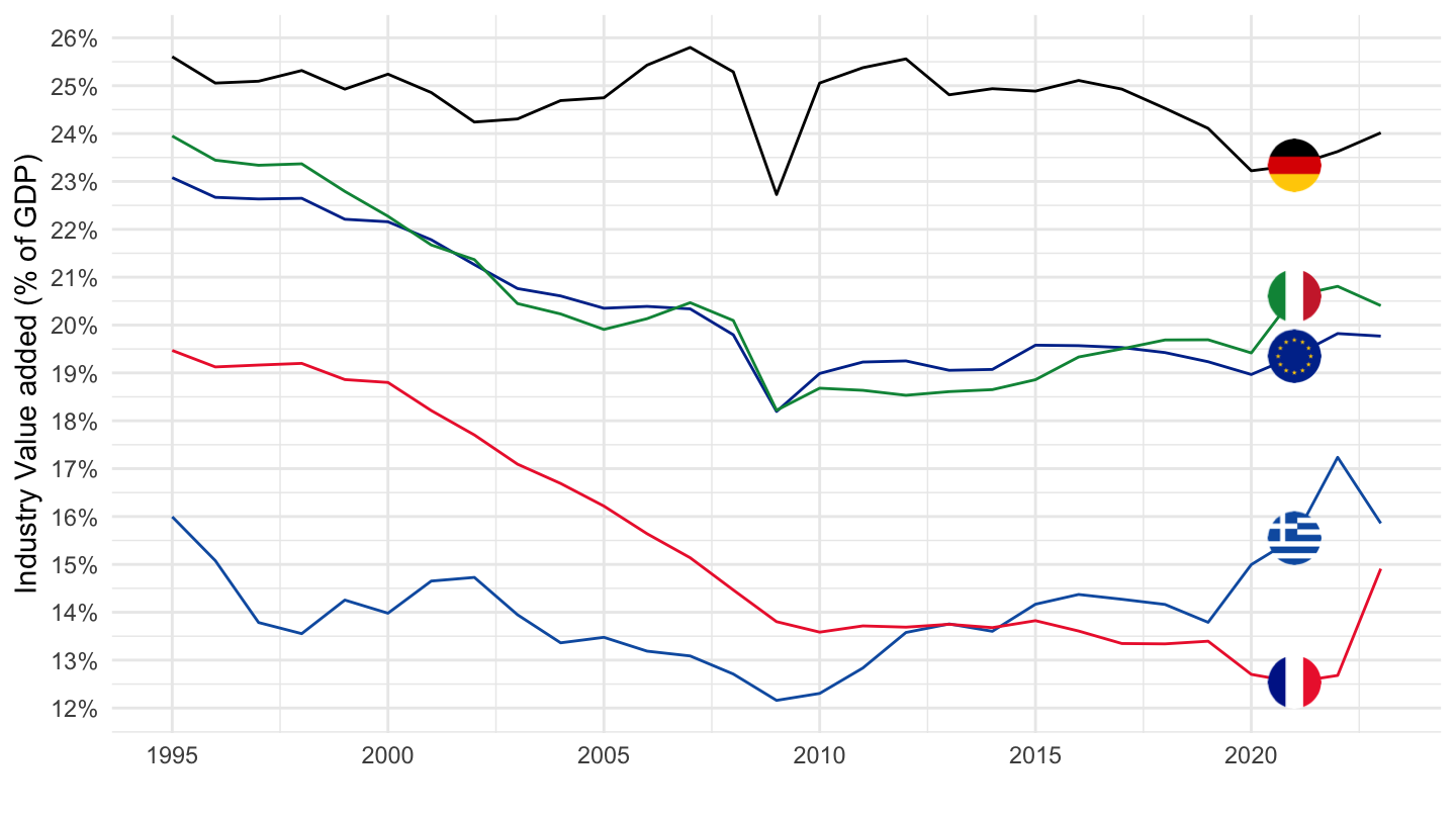

France, Germany, Greece, Italy, Portugal, Spain

All

Code

nama_10_a10 %>%
  filter(na_item == "B1G",
         nace_r2 %in% c("B-E", "TOTAL"),
         geo %in% c("FR", "DE", "EL", "ES", "IT", "PT"),
         unit == "CP_MNAC") %>%
  year_to_date() %>%
  filter(date >= as.Date("1995-01-01")) %>%
  left_join(geo, by = "geo") %>%
  select(geo,  Geo, nace_r2, date, values) %>%
  spread(nace_r2, values) %>%
  left_join(colors, by = c("Geo" = "country")) %>%
  mutate(values = `B-E`/TOTAL) %>%
  ggplot(.) + geom_line(aes(x = date, y = values, color = color)) + 
  theme_minimal() + xlab("") + ylab("Industry Value added (% of GDP)") +
  scale_color_identity() +
  scale_x_date(breaks = seq(1960, 2100, 2) %>% paste0("-01-01") %>% as.Date,
               labels = date_format("%Y")) +
  add_6flags +
  theme(legend.position = "none") +
  scale_y_continuous(breaks = 0.01*seq(-500, 200, 1),
                     labels = percent_format(accuracy = 1))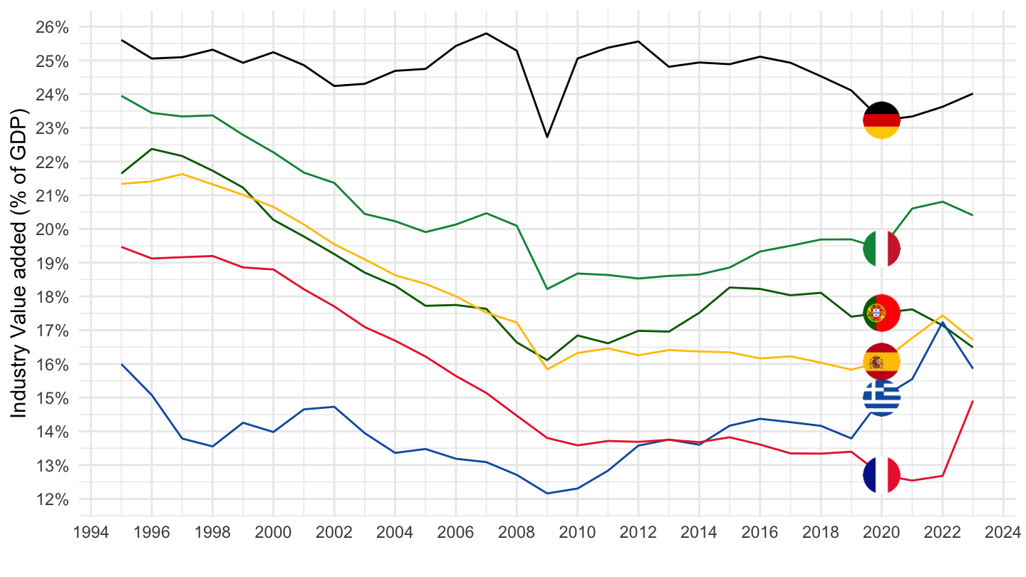

1995-

Code

nama_10_a10 %>%
  filter(na_item == "B1G",
         nace_r2 %in% c("B-E", "TOTAL"),
         geo %in% c("FR", "DE", "EL", "ES", "IT", "PT"),
         unit == "CP_MNAC") %>%
  year_to_date() %>%
  filter(date >= as.Date("1995-01-01")) %>%
  left_join(geo, by = "geo") %>%
  select(geo,  Geo, nace_r2, date, values) %>%
  spread(nace_r2, values) %>%
  left_join(colors, by = c("Geo" = "country")) %>%
  mutate(values = `B-E`/TOTAL) %>%
  ggplot(.) + geom_line(aes(x = date, y = values, color = color)) + 
  theme_minimal() + xlab("") + ylab("Industry Value added (% of GDP)") +
  scale_color_identity() +
  scale_x_date(breaks = seq(1960, 2100, 5) %>% paste0("-01-01") %>% as.Date,
               labels = date_format("%Y")) +
  add_6flags +
  theme(legend.position = "none") +
  scale_y_continuous(breaks = 0.01*seq(-500, 200, 1),
                     labels = percent_format(accuracy = 1))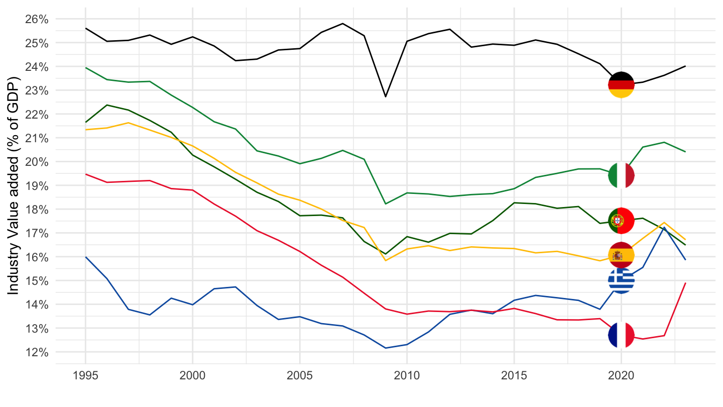

France, Luxembourg, Cyprus

1995-

Code

nama_10_a10 %>%
  filter(na_item == "B1G",
         nace_r2 %in% c("B-E", "TOTAL"),
         geo %in% c("FR", "ME", "LU", "CY", "MT", "EL"),
         unit == "CP_MNAC") %>%
  year_to_date() %>%
  filter(date >= as.Date("1995-01-01")) %>%
  left_join(geo, by = "geo") %>%
  select(geo,  Geo, nace_r2, date, values) %>%
  spread(nace_r2, values) %>%
  left_join(colors, by = c("Geo" = "country")) %>%
  mutate(values = `B-E`/TOTAL) %>%
  ggplot(.) + geom_line(aes(x = date, y = values, color = color)) + 
  theme_minimal() + xlab("") + ylab("Industry Value added (% of GDP)") +
  scale_color_identity() +
  scale_x_date(breaks = seq(1960, 2100, 5) %>% paste0("-01-01") %>% as.Date,
               labels = date_format("%Y")) +
  add_6flags +
  theme(legend.position = "none") +
  scale_y_continuous(breaks = 0.01*seq(-500, 200, 1),
                     labels = percent_format(accuracy = 1))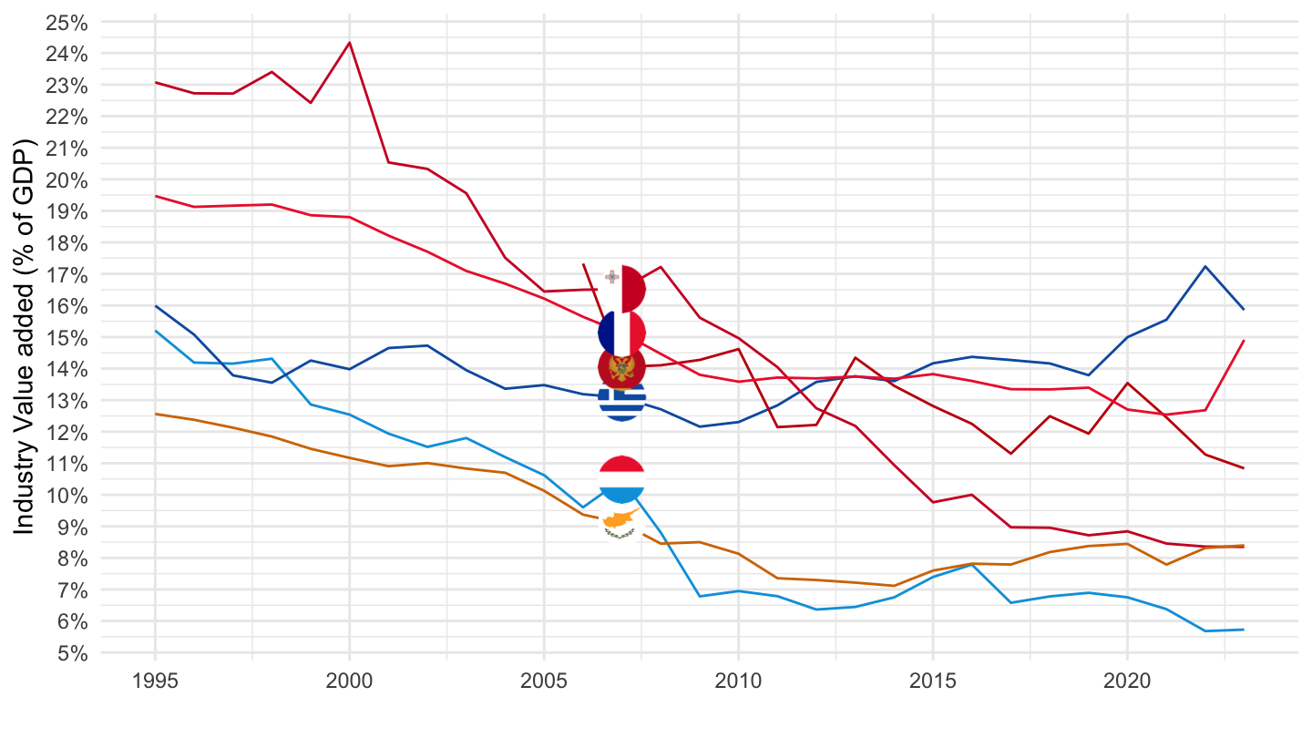

Greece, Portugal, Spain

Code

nama_10_a10 %>%
  filter(na_item == "B1G",
         nace_r2 %in% c("B-E", "TOTAL"),
         geo %in% c("EL", "PT", "ES"),
         unit == "CP_MNAC") %>%
  year_to_date() %>%
  left_join(geo, by = "geo") %>%
  select(Geo, nace_r2, date, values) %>%
  spread(nace_r2, values) %>%
  ggplot(.) + geom_line(aes(x = date, y = `B-E`/TOTAL, color = Geo)) + 
  theme_minimal() + xlab("") + ylab("Manufacturing Value added (% of GDP)") +
  scale_color_manual(values = c("#0D5EAF", "#006600", "#C60B1E")) +
  scale_x_date(breaks = seq(1960, 2025, 5) %>% paste0("-01-01") %>% as.Date,
               labels = date_format("%Y")) +
  geom_image(data = . %>%
               filter(date == as.Date("2016-01-01")) %>%
               mutate(date = as.Date("2016-01-01"),
                      image = paste0("../../icon/flag/", str_to_lower(Geo), ".png")),
             aes(x = date, y = `B-E`/TOTAL, image = image), asp = 1.5) +
  theme(legend.position = "none") +
  scale_y_continuous(breaks = 0.01*seq(-500, 200, 1),
                     labels = percent_format(accuracy = 1))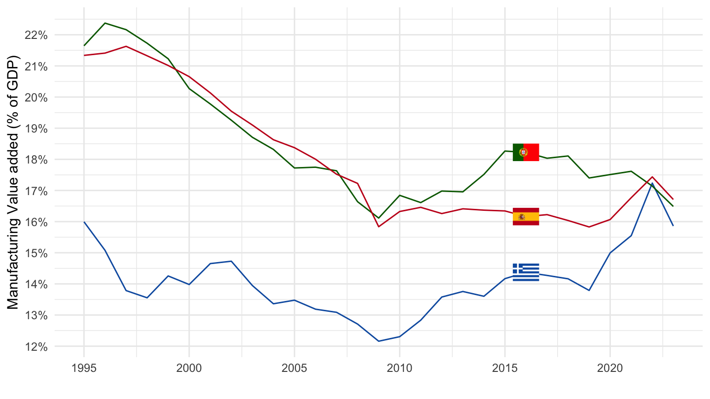

1995-2018

Code

nama_10_a10 %>%
  filter(na_item == "B1G",
         nace_r2 %in% c("B-E", "TOTAL"),
         geo %in% c("EA", "FR", "DE", "IT", "ES", "NL", "AT", "FI"),
         unit == "CP_MNAC") %>%
  year_to_date() %>%
  filter(date >= as.Date("1995-01-01"),
         date <= as.Date("2019-01-01")) %>%
  left_join(geo, by = "geo") %>%
  select(geo, Geo, nace_r2, date, values) %>%
  spread(nace_r2, values) %>%
  mutate(values = `B-E`/TOTAL) %>%
  group_by(date) %>%
  mutate(values = values /values[geo == "EA"]) %>%
  filter(geo != "EA") %>%
  group_by(geo) %>%
  mutate(values = 100*values / values[date == as.Date("1995-01-01")]) %>%
  left_join(colors, by = c("Geo" = "country")) %>%
  mutate(color = ifelse(geo == "FR", color2, color)) %>%
  ggplot(.) + geom_line(aes(x = date, y = values, color = color)) + 
  theme_minimal() + xlab("") + ylab("Valeur ajoutée manuf. par rapport à la Zone €") +
  scale_color_identity() + add_7flags +
  theme(legend.position = "none") +
  scale_x_date(breaks = seq(1995, 2025, 5) %>% paste0("-01-01") %>% as.Date,
               labels = date_format("%Y")) +
  scale_y_continuous(breaks = seq(0, 200, 5)) +
  theme(legend.position = "none") +
  geom_hline(yintercept = 100, linetype = "dashed")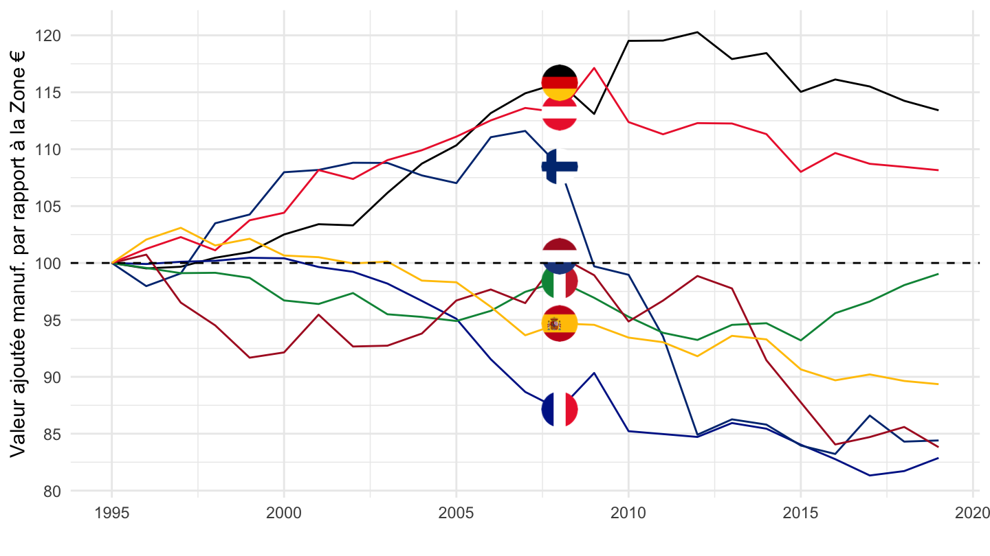

1995-

Code

nama_10_a10 %>%
  filter(na_item == "B1G",
         nace_r2 %in% c("B-E", "TOTAL"),
         geo %in% c("EA", "FR", "DE", "IT", "ES", "NL", "AT", "PL", "CZ"),
         unit == "CP_MNAC") %>%
  year_to_date() %>%
  filter(date >= as.Date("1995-01-01"),
         date <= as.Date("2019-01-01")) %>%
  left_join(geo, by = "geo") %>%
  select(geo, Geo, nace_r2, date, values) %>%
  spread(nace_r2, values) %>%
  mutate(values = `B-E`/TOTAL) %>%
  group_by(date) %>%
  mutate(values = values /values[geo == "EA"]) %>%
  filter(geo != "EA") %>%
  group_by(geo) %>%
  mutate(values = 100*values / values[date == as.Date("1995-01-01")]) %>%
  left_join(colors, by = c("Geo" = "country")) %>%
  mutate(color = ifelse(geo == "FR", color2, color)) %>%
  ggplot(.) + geom_line(aes(x = date, y = values, color = color)) + 
  theme_minimal() + xlab("") + ylab("Valeur ajoutée manuf. par rapport à la Zone €") +
  scale_color_identity() +
  add_8flags +
  theme(legend.position = "none") +
  scale_x_date(breaks = seq(1995, 2025, 5) %>% paste0("-01-01") %>% as.Date,
               labels = date_format("%Y")) +
  scale_y_log10(breaks = seq(0, 200, 5)) +
  theme(legend.position = "none") +
  geom_hline(yintercept = 100, linetype = "dashed")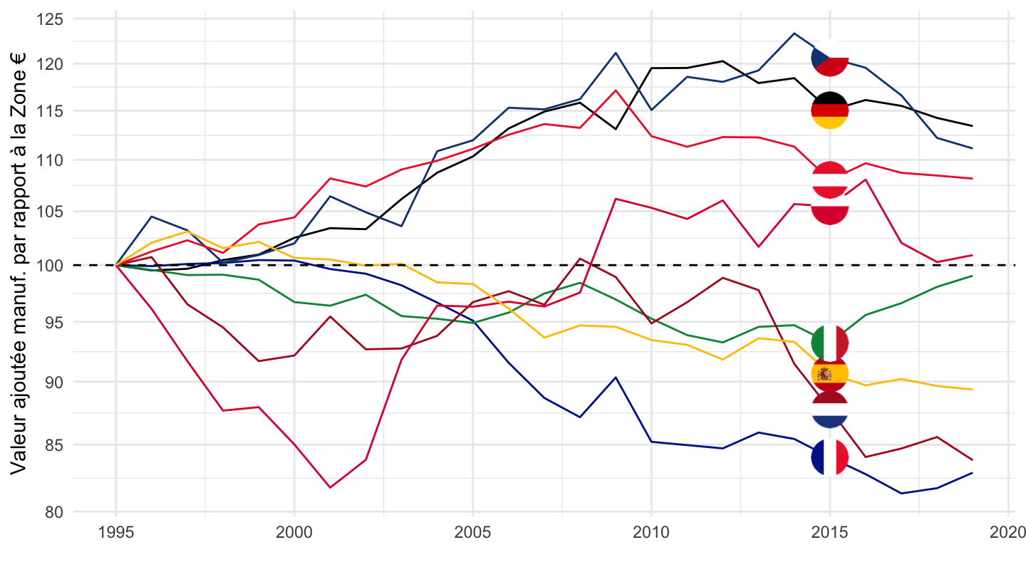

2000-2018

Code

nama_10_a10 %>%
  filter(na_item == "B1G",
         nace_r2 %in% c("B-E", "TOTAL"),
         geo %in% c("EA", "FR", "DE", "IT", "ES", "NL", "AT", "FI"),
         unit == "CP_MNAC") %>%
  year_to_date() %>%
  filter(date >= as.Date("2000-01-01"),
         date <= as.Date("2019-01-01")) %>%
  left_join(geo, by = "geo") %>%
  select(geo, Geo, nace_r2, date, values) %>%
  spread(nace_r2, values) %>%
  mutate(values = `B-E`/TOTAL) %>%
  group_by(date) %>%
  mutate(values = values /values[geo == "EA"]) %>%
  filter(geo != "EA") %>%
  group_by(geo) %>%
  mutate(values = 100*values / values[date == as.Date("2000-01-01")]) %>%
  left_join(colors, by = c("Geo" = "country")) %>%
  mutate(color = ifelse(geo == "FR", color2, color)) %>%
  ggplot(.) + geom_line(aes(x = date, y = values, color = color)) + 
  theme_minimal() + xlab("") + ylab("Valeur ajoutée manuf. par rapport à la Zone €") +
  scale_color_identity() + add_7flags +
  scale_x_date(breaks = seq(1960, 2020, 1) %>% paste0("-01-01") %>% as.Date,
               labels = date_format("%Y")) +
  scale_y_continuous(breaks = seq(0, 200, 5)) +
  theme(legend.position = "none") +
  geom_hline(yintercept = 100, linetype = "dashed")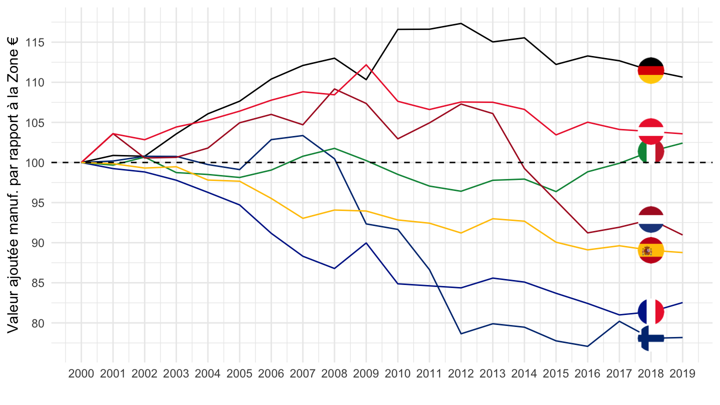

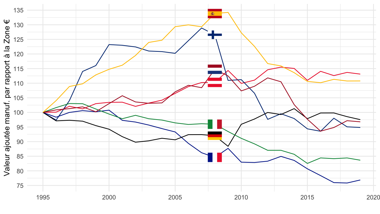
Industry

1995-2018

Code

nama_10_a10 %>%
  filter(na_item == "B1G",
         nace_r2 == "B-E",
         geo %in% c("EA", "FR", "DE", "IT", "ES", "NL", "AT", "FI"),
         unit == "CP_MNAC") %>%
  year_to_date() %>%
  filter(date >= as.Date("1995-01-01"),
         date <= as.Date("2019-01-01")) %>%
  left_join(geo, by = "geo") %>%
  group_by(date) %>%
  mutate(values = values /values[geo == "EA"]) %>%
  filter(geo != "EA") %>%
  group_by(geo) %>%
  mutate(values = 100*values/values[date == as.Date("1995-01-01")]) %>%
  ggplot(.) + geom_line(aes(x = date, y = values, color = Geo)) + 
  theme_minimal() + xlab("") + ylab("Valeur ajoutée manuf. par rapport à la Zone €") +
  scale_color_manual(values = c("#ED2939", "#003580", "#002395", "#000000",
                                "#009246", "#AE1C28", "#FFC400")) +
  scale_x_date(breaks = seq(1960, 2020, 5) %>% paste0("-01-01") %>% as.Date,
               labels = date_format("%Y")) +
  geom_image(data = . %>%
               filter(date == as.Date("2008-01-01")) %>%
               mutate(image = paste0("../../icon/flag/", str_to_lower(Geo), ".png")),
             aes(x = date, y = values, image = image), asp = 1.5) +
  scale_y_continuous(breaks = seq(0, 200, 5)) +
  theme(legend.position = "none")