Code
tibble(DOWNLOAD_TIME = as.Date(file.info("~/iCloud/website/data/eurostat/ei_isin_m.RData")$mtime)) %>%
print_table_conditional()| DOWNLOAD_TIME |
|---|
| 2026-04-14 |
Data - Eurostat
tibble(DOWNLOAD_TIME = as.Date(file.info("~/iCloud/website/data/eurostat/ei_isin_m.RData")$mtime)) %>%
print_table_conditional()| DOWNLOAD_TIME |
|---|
| 2026-04-14 |
ei_isin_m %>%
  group_by(time) %>%
  summarise(Nobs = n()) %>%
  arrange(desc(time)) %>%
  head(1) %>%
print_table_conditional()| time | Nobs |
|---|---|
| 2026M03 | 69 |
load_data("eurostat/indic_fr.RData")
ei_isin_m %>%
  left_join(indic, by = "indic") %>%
  group_by(indic, Indic) %>%
  summarise(Nobs = n()) %>%
  arrange(-Nobs) %>%
{if (is_html_output()) print_table(.) else .}| indic | Indic | Nobs |
|---|---|---|
| IS-IP | Indice de production | 614104 |
| IS-ITT | Indice du chiffre d'affaires - total | 584852 |
| IS-ITD | Indice du chiffre d'affaires - marché intérieur | 573620 |
| IS-ITND | Indice du chiffre d'affaires - marché extérieur | 370723 |
| IS-PPI | Prix à la production de l'indice du marché intérieur (indice des prix à la production) (NSA) | 266928 |
| IS-WSI | Indice des salaires et traitements bruts | 137202 |
| IS-IMPR | Indices des prix à l'importation (NSA) | 112676 |
| IS-EPI | Indice du nombre de personnes occupées | 112290 |
| IS-HWI | Indice des heures travaillées | 110070 |
| IS-IMPX | Indices des prix à l'importation - hors zone euro (NSA) | 71637 |
| IS-IMPZ | Indices des prix à l'importation - zone euro (NSA) | 65593 |
load_data("eurostat/indic.RData")
ei_isin_m %>%
  left_join(nace_r2, by = "nace_r2") %>%
  group_by(nace_r2, Nace_r2) %>%
  summarise(Nobs = n()) %>%
{if (is_html_output()) datatable(., filter = 'top', rownames = F) else .}ei_isin_m %>%
left_join(s_adj, by = "s_adj") %>%
group_by(s_adj, S_adj) %>%
summarise(Nobs = n()) %>%
arrange(-Nobs) %>%
{if (is_html_output()) print_table(.) else .}| s_adj | S_adj | Nobs |
|---|---|---|
| NSA | Unadjusted data (i.e. neither seasonally adjusted nor calendar adjusted data) | 1229714 |
| SCA | Seasonally and calendar adjusted data | 1081699 |
| CA | Calendar adjusted data, not seasonally adjusted data | 708282 |
ei_isin_m %>%
  left_join(unit, by = "unit") %>%
  group_by(unit, Unit) %>%
  summarise(Nobs = n()) %>%
  arrange(-Nobs) %>%
{if (is_html_output()) print_table(.) else .}| unit | Unit | Nobs |
|---|---|---|
| I2021 | Index, 2021=100 | 1554675 |
| I2015 | Index, 2015=100 | 1465020 |
ei_isin_m %>%
  left_join(geo, by = "geo") %>%
  group_by(geo, Geo) %>%
  summarise(Nobs = n()) %>%
  arrange(-Nobs) %>%
  mutate(Geo = ifelse(geo == "DE", "Germany", Geo)) %>%
  mutate(Flag = gsub(" ", "-", str_to_lower(Geo)),
         Flag = paste0('<img src="../../bib/flags/vsmall/', Flag, '.png" alt="Flag">')) %>%
  select(Flag, everything()) %>%
{if (is_html_output()) datatable(., filter = 'top', rownames = F, escape = F) else .}ei_isin_m %>%
group_by(time) %>%
summarise(Nobs = n()) %>%
arrange(desc(time)) %>%
{if (is_html_output()) datatable(., filter = 'top', rownames = F) else .}ei_isin_m %>%
filter(nace_r2 == "C",
indic == "IS-IP",
geo %in% c("FR", "DE", "IT"),
s_adj == "SCA") %>%
select(geo, time, values) %>%
group_by(geo) %>%
mutate(values = 100*values/values[time == "1997M01"]) %>%
left_join(geo, by = "geo") %>%
mutate(Geo = ifelse(geo == "DE", "Germany", Geo)) %>%
month_to_date %>%
ggplot() + ylab("Industrial Production") + xlab("") + theme_minimal() +
geom_line(aes(x = date, y = values, color = Geo)) + add_3flags +
scale_color_manual(values = c("#0055a4", "#000000", "#008c45")) +
scale_x_date(breaks = seq(1920, 2025, 2) %>% paste0("-01-01") %>% as.Date,
labels = date_format("%y")) +
scale_y_log10(breaks = seq(-60, 300, 10))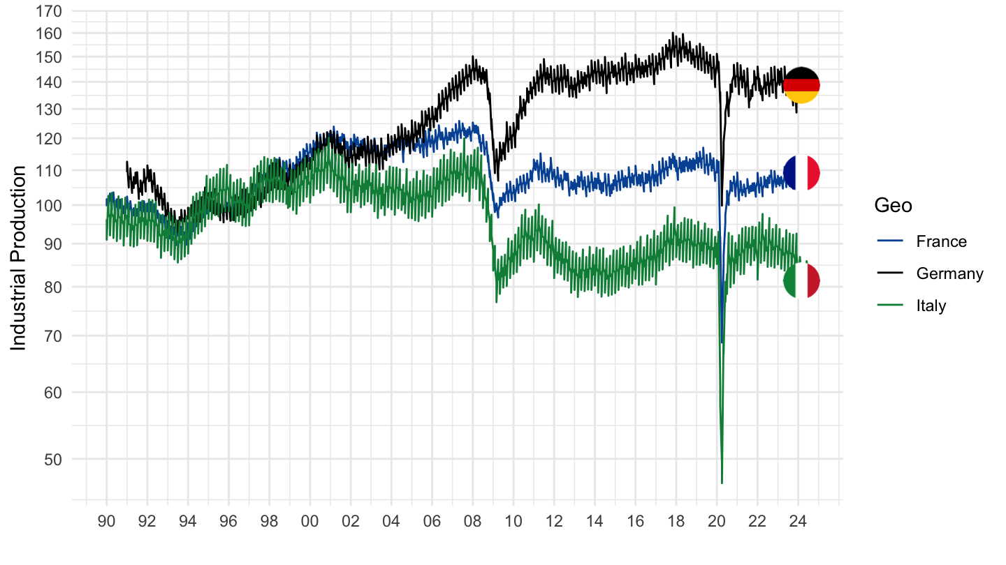
Turnover indices serve to provide a monthly measurement of trends in the activity of companies in the industrial, construction, retail, personal services, wholesale and miscellaneous services to enterprises sectors. They are elaborated each month from the monthly declarations (CA3) made by enterprises falling within the normal tax arrangements for the payment of value added tax (VAT). These indices are determined at the finest level of the French classification of activities (that is, the sub-classes of NAF rev.2) then aggregated to provide indices for the different levels of the composite nomenclatures (NA, NACE). The resultant indices are in volume in the retail and personal services sectors, and in value in the other sectors. The series are disseminated raw or seasonally and calendar effect adjusted.
ei_isin_m %>%
  filter(nace_r2 == "C",
         indic == "IS-ITT",
         geo %in% c("FR", "DE", "IT"),
         s_adj == "SCA") %>%
  filter(!is.na(values)) %>%
  select(geo, time, values) %>%
  group_by(geo) %>%
  mutate(values = 100*values/values[time == "2005M01"]) %>%
  left_join(geo, by = "geo") %>%
  mutate(Geo = ifelse(geo == "DE", "Germany", Geo)) %>%
  month_to_date %>%
  ggplot() + ylab("Turnover index - total") + xlab("") + theme_minimal() +
  geom_line(aes(x = date, y = values, color = Geo)) + add_3flags +
  scale_color_manual(values = c("#0055a4", "#000000", "#008c45")) +
  scale_x_date(breaks = seq(1920, 2025, 2) %>% paste0("-01-01") %>% as.Date,
               labels = date_format("%y")) +
  theme(legend.position = "none") +
  scale_y_log10(breaks = seq(-60, 300, 10))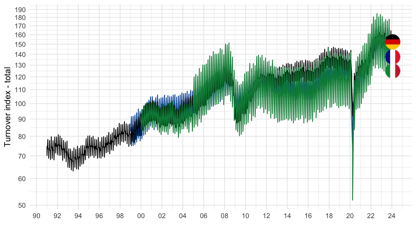
ei_isin_m %>%
  filter(nace_r2 == "C",
         indic == "IS-ITD",
         geo %in% c("FR", "DE", "IT"),
         s_adj == "SCA") %>%
  select(geo, time, values) %>%
  group_by(geo) %>%
  mutate(values = 100*values/values[time == "2005M01"]) %>%
  left_join(geo, by = "geo") %>%
  mutate(Geo = ifelse(geo == "DE", "Germany", Geo)) %>%
  month_to_date %>%
  ggplot() + ylab("Turnover index - domestic market") + xlab("") + theme_minimal() +
  geom_line(aes(x = date, y = values, color = Geo)) + add_3flags +
  scale_color_manual(values = c("#0055a4", "#000000", "#008c45")) +
  scale_x_date(breaks = seq(1920, 2025, 2) %>% paste0("-01-01") %>% as.Date,
               labels = date_format("%y")) +
  theme(legend.position = "none") +
  scale_y_log10(breaks = seq(-60, 300, 10))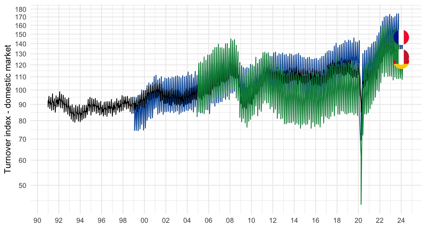
ei_isin_m %>%
  filter(nace_r2 == "C",
         indic == "IS-ITND",
         geo %in% c("FR", "DE", "IT"),
         s_adj == "SCA") %>%
  select(geo, time, values) %>%
  group_by(geo) %>%
  mutate(values = 100*values/values[time == "2005M01"]) %>%
  left_join(geo, by = "geo") %>%
  mutate(Geo = ifelse(geo == "DE", "Germany", Geo)) %>%
  month_to_date %>%
  ggplot() + ylab("Turnover index - non-domestic market") + xlab("") + theme_minimal() +
  geom_line(aes(x = date, y = values, color = Geo)) +  add_3flags +
  scale_color_manual(values = c("#0055a4", "#000000", "#008c45")) +
  scale_x_date(breaks = seq(1920, 2025, 2) %>% paste0("-01-01") %>% as.Date,
               labels = date_format("%y")) +
  theme(legend.position = "none") +
  scale_y_log10(breaks = seq(-60, 300, 10))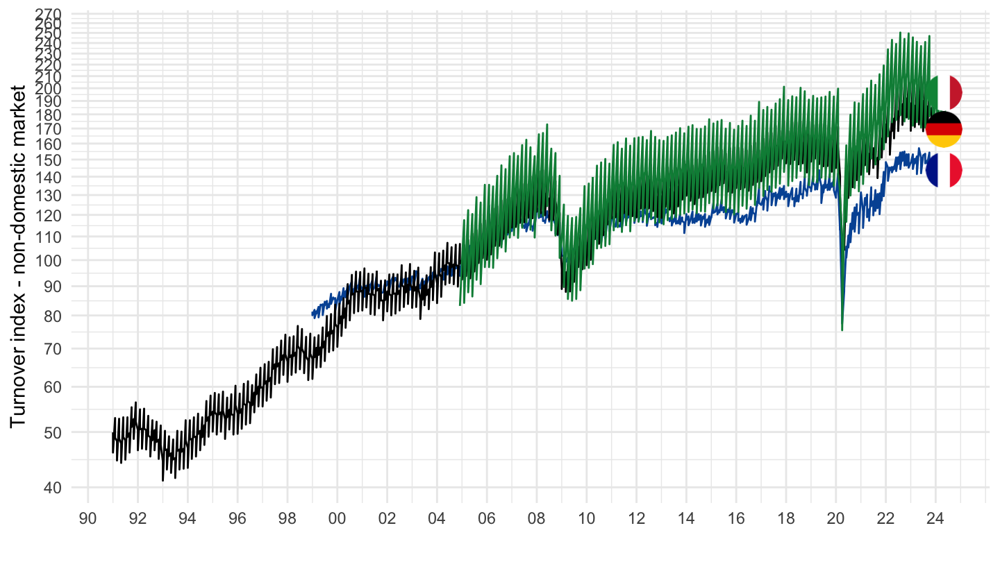
ei_isin_m %>%
  filter(nace_r2 == "MIG_DCOG",
         indic == "IS-IP",
         geo %in% c("FR", "DE", "IT"),
         s_adj == "SCA") %>%
  select(geo, time, values) %>%
  group_by(geo) %>%
  mutate(values = 100*values/values[time == "1997M01"]) %>%
  left_join(geo, by = "geo") %>%
  mutate(Geo = ifelse(geo == "DE", "Germany", Geo)) %>%
  month_to_date %>%
  left_join(colors, by = c("Geo" = "country")) %>%
  ggplot() + ylab("Durable Goods - Industrial Production") + xlab("") + theme_minimal() +
  geom_line(aes(x = date, y = values, color = color)) + add_3flags +
  scale_color_identity() +
  scale_x_date(breaks = seq(1920, 2025, 2) %>% paste0("-01-01") %>% as.Date,
               labels = date_format("%y")) +
  theme(legend.position = "none") +
  scale_y_log10(breaks = seq(-60, 300, 10))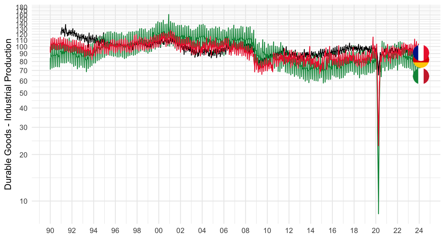
ei_isin_m %>%
  filter(nace_r2 == "MIG_COG",
         indic == "IS-IP",
         geo %in% c("FR", "DE", "IT"),
         s_adj == "SCA") %>%
  select(geo, time, values) %>%
  group_by(geo) %>%
  mutate(values = 100*values/values[time == "1997M01"]) %>%
  left_join(geo, by = "geo") %>%
  mutate(Geo = ifelse(geo == "DE", "Germany", Geo)) %>%
  month_to_date %>%
  ggplot() + ylab("Consumer Goods - Industrial Production") + xlab("") + theme_minimal() +
  geom_line(aes(x = date, y = values, color = Geo)) + add_3flags +
  scale_color_manual(values = c("#0055a4", "#000000", "#008c45")) +
  scale_x_date(breaks = seq(1920, 2025, 2) %>% paste0("-01-01") %>% as.Date,
               labels = date_format("%y")) +
  theme(legend.position = "none") +
  scale_y_log10(breaks = seq(-60, 300, 10))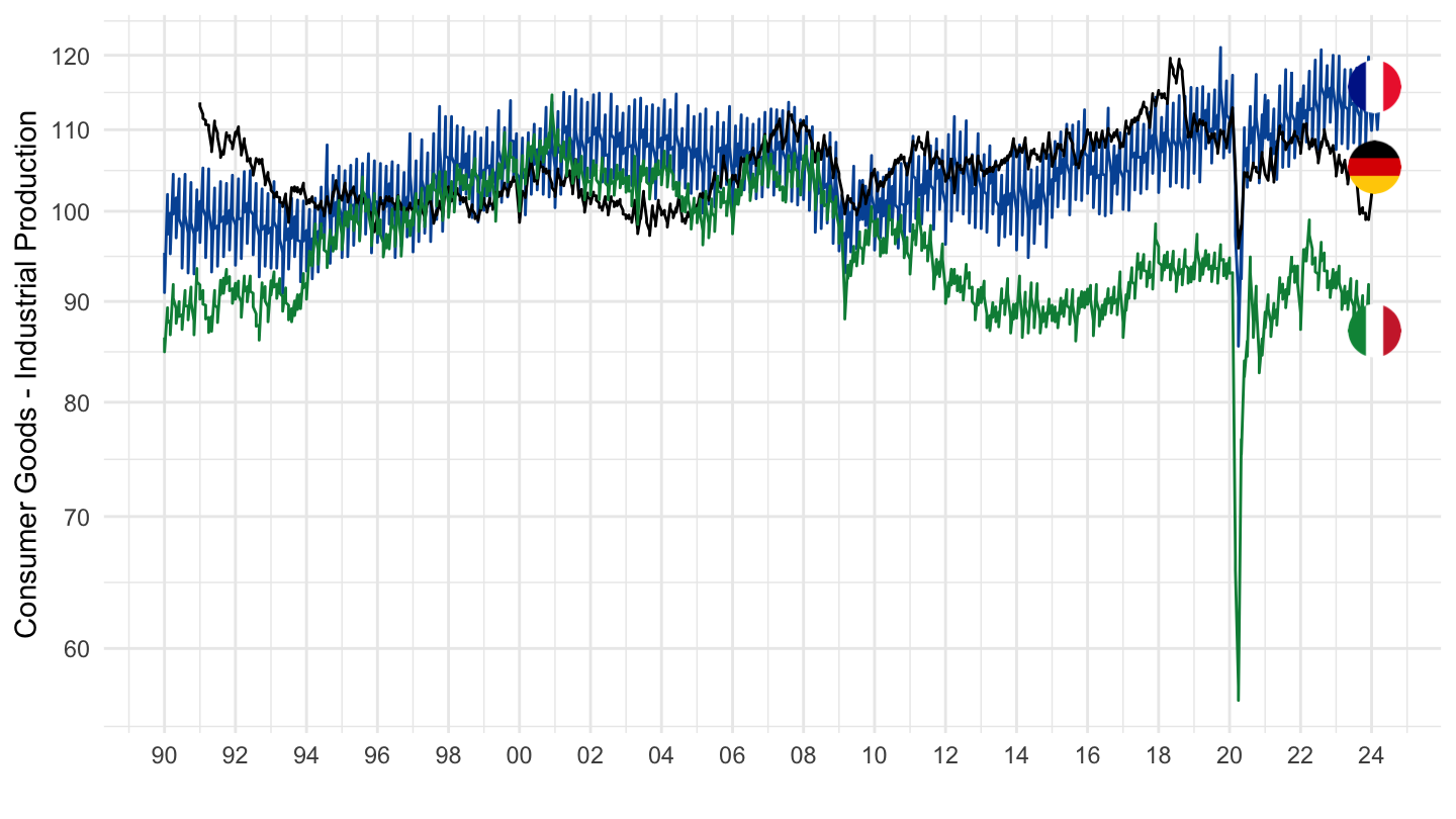
ei_isin_m %>%
  filter(nace_r2 == "MIG_CAG",
         indic == "IS-IP",
         geo %in% c("FR", "DE", "IT"),
         s_adj == "SCA") %>%
  select(geo, time, values) %>%
  group_by(geo) %>%
  mutate(values = 100*values/values[time == "1997M01"]) %>%
  left_join(geo, by = "geo") %>%
  mutate(Geo = ifelse(geo == "DE", "Germany", Geo)) %>%
  month_to_date %>%
  ggplot() + ylab("Capital Goods - Industrial Production") + xlab("") + theme_minimal() +
  geom_line(aes(x = date, y = values, color = Geo)) + add_3flags +
  scale_color_manual(values = c("#0055a4", "#000000", "#008c45")) +
  scale_x_date(breaks = seq(1920, 2025, 2) %>% paste0("-01-01") %>% as.Date,
               labels = date_format("%y")) +
  theme(legend.position = "none") +
  scale_y_log10(breaks = seq(-60, 300, 10))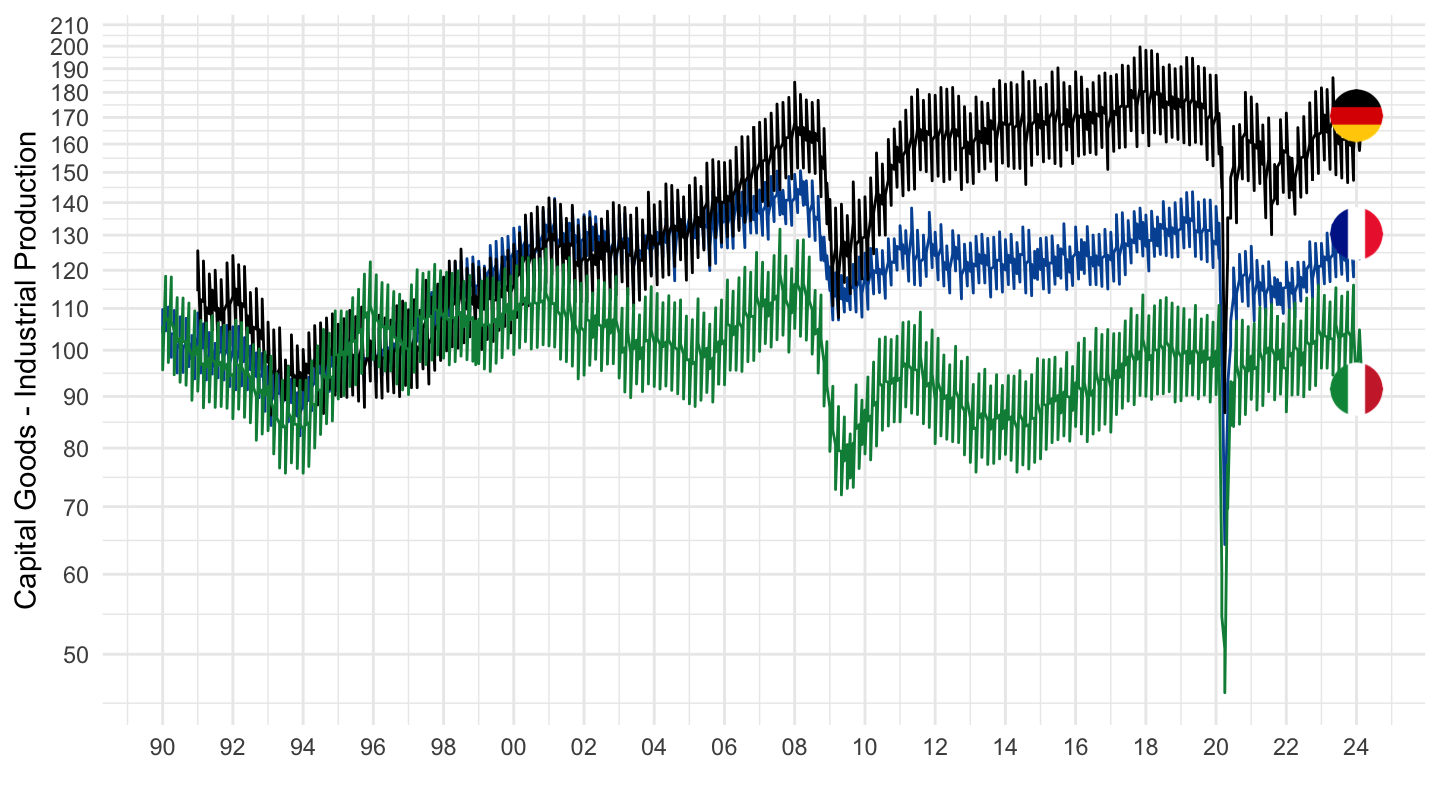
ei_isin_m %>%
  filter(nace_r2 == "C",
         indic == "IS-ITT",
         geo %in% c("FR", "DE", "IT", "ES"),
         s_adj == "SCA") %>%
  select(geo, time, values) %>%
  group_by(geo) %>%
  mutate(values = 100*values/values[time == "2020M02"]) %>%
  left_join(geo, by = "geo") %>%
  mutate(Geo = ifelse(geo == "DE", "Germany", Geo)) %>%
  month_to_date %>%
  filter(date >= as.Date("2020-02-01")) %>%
  ggplot() + ylab("Turnover index - all") + xlab("") + theme_minimal() +
  geom_line(aes(x = date, y = values, color = Geo)) + add_4flags +
  scale_color_manual(values = c("#0055a4", "#000000", "#008c45", "#C60B1E")) +
  scale_x_date(breaks = "2 months",
               labels = date_format("%b %y")) +
  theme(legend.position = "none") +
  scale_y_log10(breaks = seq(-60, 300, 10))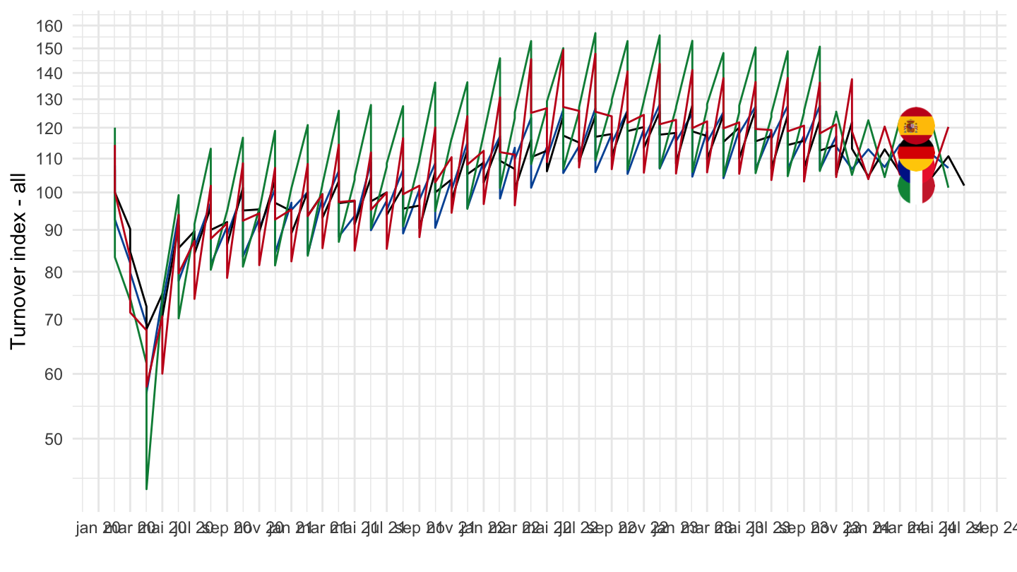
ei_isin_m %>%
  filter(nace_r2 == "C",
         indic == "IS-ITT",
         geo %in% c("FR", "DE", "IT", "ES"),
         s_adj == "SCA") %>%
  select(geo, time, values) %>%
  group_by(geo) %>%
  mutate(values = 100*values/values[time == "2020M02"]) %>%
  left_join(geo, by = "geo") %>%
  month_to_date %>%
  filter(date >= as.Date("2020-02-01")) %>%
  group_by(Geo) %>%
  arrange(date) %>%
  mutate(values = values-100,
         values = cumsum(values)) %>%
  ggplot() + ylab("Turnover index - all (Cum. Sum)") + xlab("") + theme_minimal() +
  geom_line(aes(x = date, y = values, color = Geo)) + add_4flags +
  scale_color_manual(values = c("#0055a4", "#000000", "#008c45", "#C60B1E")) +
  scale_x_date(breaks = "2 months",
               labels = date_format("%b %y")) +
  theme(legend.position = "none") +
  scale_y_continuous(breaks = seq(-300, 300, 10))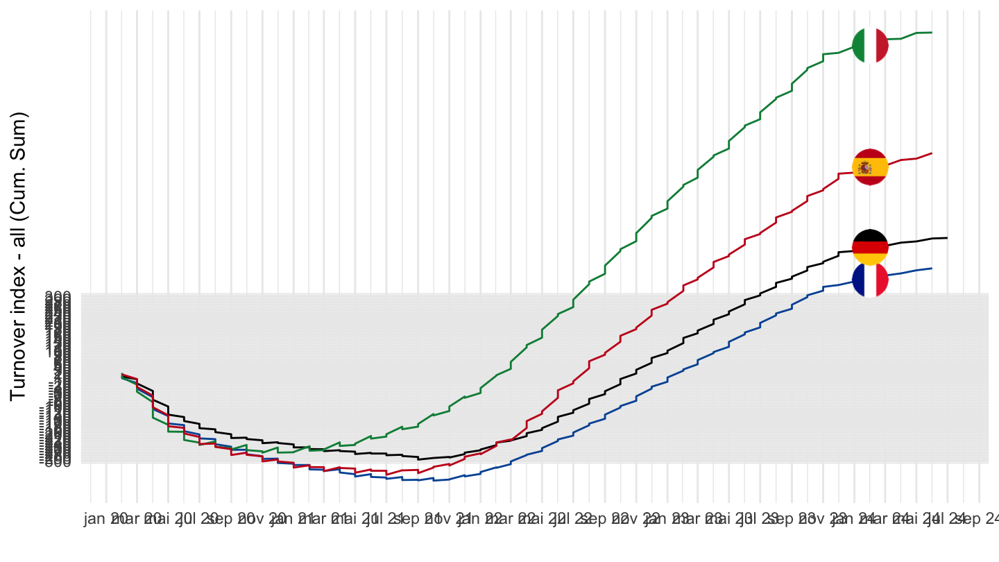
ei_isin_m %>%
  filter(nace_r2 == "C",
         indic == "IS-ITND",
         geo %in% c("FR", "DE", "IT", "ES"),
         s_adj == "SCA") %>%
  select(geo, time, values) %>%
  group_by(geo) %>%
  mutate(values = 100*values/values[time == "2020M02"]) %>%
  left_join(geo, by = "geo") %>%
  mutate(Geo = ifelse(geo == "DE", "Germany", Geo)) %>%
  month_to_date %>%
  filter(date >= as.Date("2020-02-01")) %>%
  ggplot() + ylab("Turnover index - external market") + xlab("") + theme_minimal() +
  geom_line(aes(x = date, y = values, color = Geo)) + add_3flags +
  scale_color_manual(values = c("#0055a4", "#000000", "#008c45", "#C60B1E")) +
  scale_x_date(breaks = "1 month",
               labels = date_format("%b %y")) +
  theme(legend.position = "none") +
  scale_y_log10(breaks = seq(-60, 300, 10))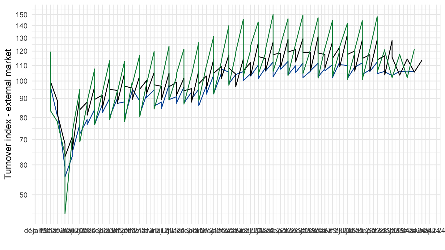
ei_isin_m %>%
  filter(nace_r2 == "C",
         indic == "IS-ITND",
         geo %in% c("FR", "DE", "IT", "ES"),
         s_adj == "SCA") %>%
  select(geo, time, values) %>%
  group_by(geo) %>%
  mutate(values = 100*values/values[time == "2020M02"]) %>%
  left_join(geo, by = "geo") %>%
  month_to_date %>%
  filter(date >= as.Date("2020-02-01")) %>%
  group_by(Geo) %>%
  arrange(date) %>%
  mutate(values = values-100,
         values = cumsum(values)) %>%
  ggplot() + ylab("Turnover index - external market (Cum. Sum)") + xlab("") + theme_minimal() +
  geom_line(aes(x = date, y = values, color = Geo)) + add_4flags +
  scale_color_manual(values = c("#0055a4", "#000000", "#008c45", "#C60B1E")) +
  scale_x_date(breaks = "1 month",
               labels = date_format("%b %y")) +
  theme(legend.position = "none") +
  scale_y_continuous(breaks = seq(-300, 300, 10))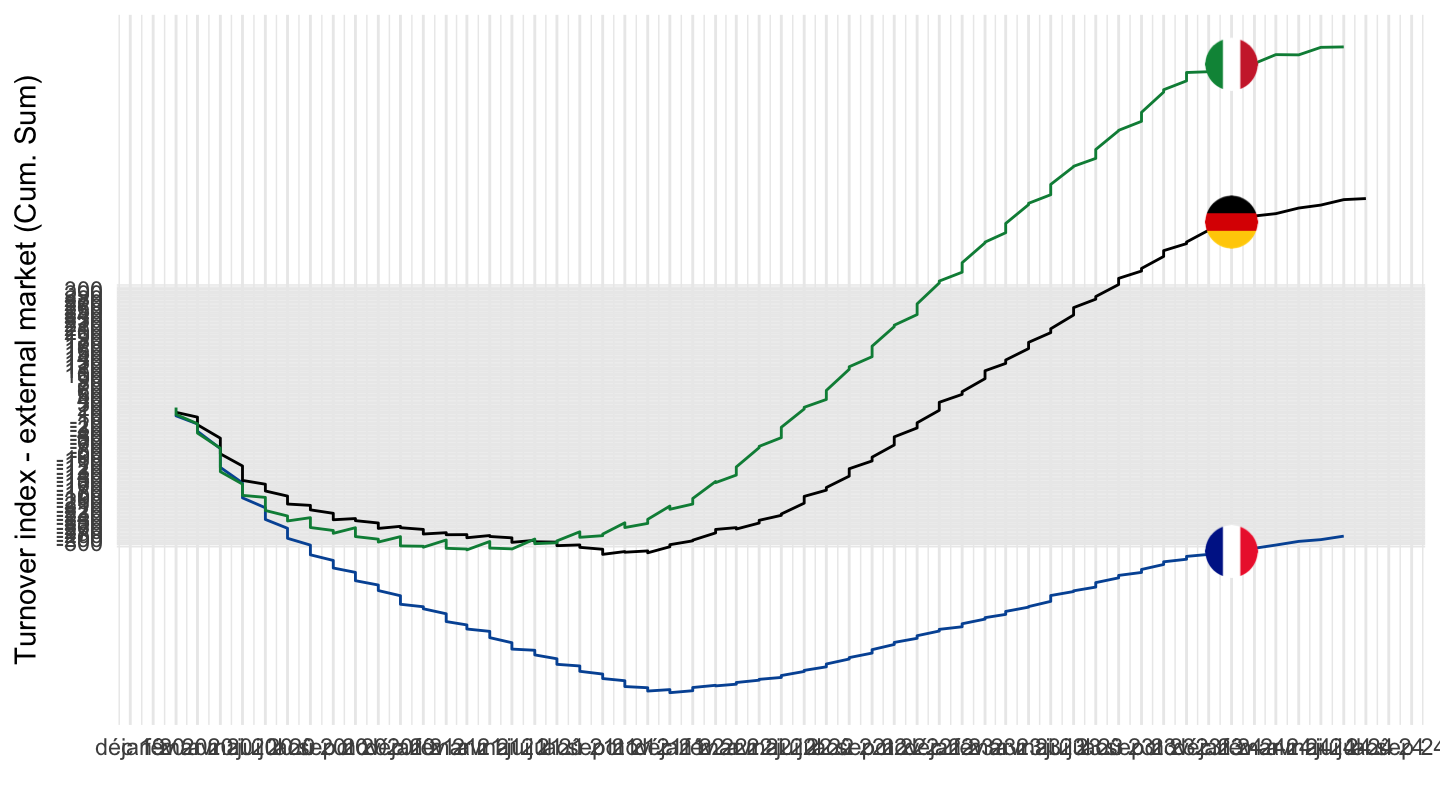
ei_isin_m %>%
  filter(nace_r2 == "C",
         indic == "IS-ITD",
         geo %in% c("FR", "DE", "IT", "ES"),
         s_adj == "SCA") %>%
  select(geo, time, values) %>%
  group_by(geo) %>%
  mutate(values = 100*values/values[time == "2020M02"]) %>%
  left_join(geo, by = "geo") %>%
  mutate(Geo = ifelse(geo == "DE", "Germany", Geo)) %>%
  month_to_date %>%
  filter(date >= as.Date("2020-02-01")) %>%
  ggplot() + ylab("Turnover index - internal market") + xlab("") + theme_minimal() +
  geom_line(aes(x = date, y = values, color = Geo)) + add_4flags +
  scale_color_manual(values = c("#0055a4", "#000000", "#008c45", "#C60B1E")) +
  scale_x_date(breaks = "1 month",
               labels = date_format("%b %y")) +
  theme(legend.position = "none") +
  scale_y_log10(breaks = seq(-60, 300, 10))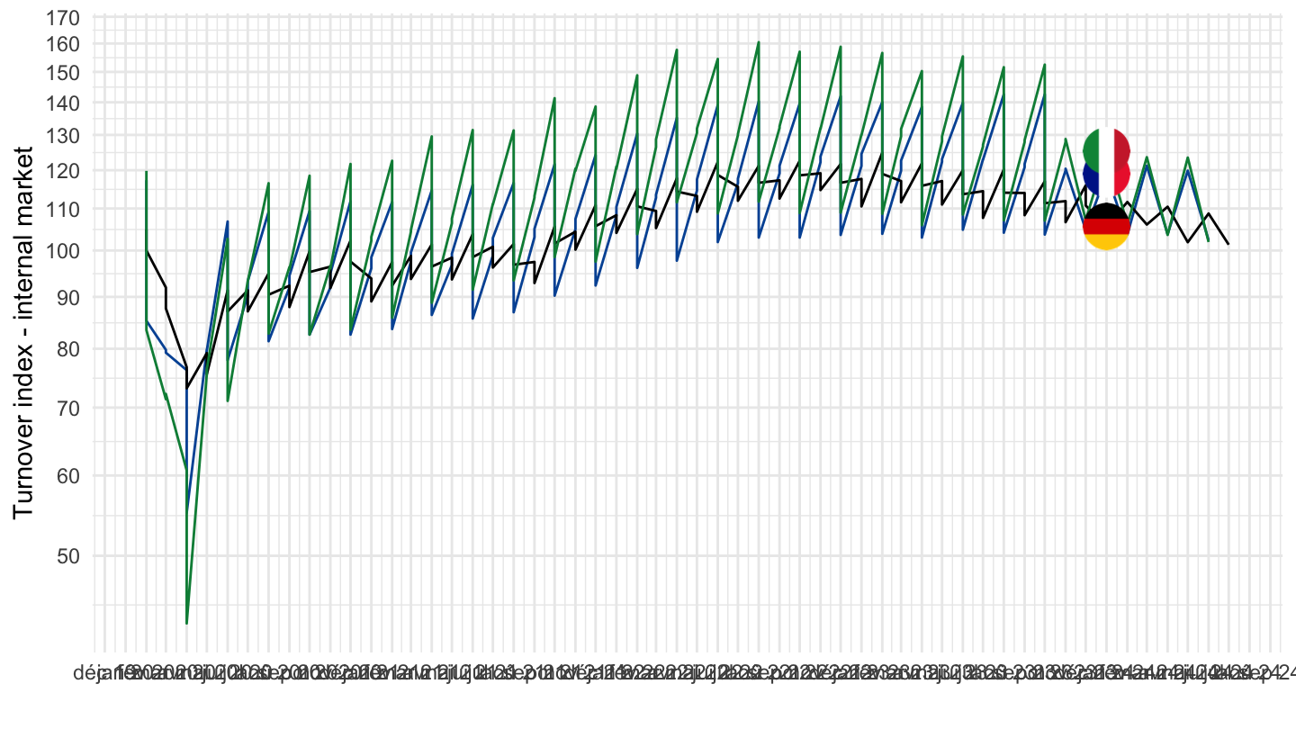
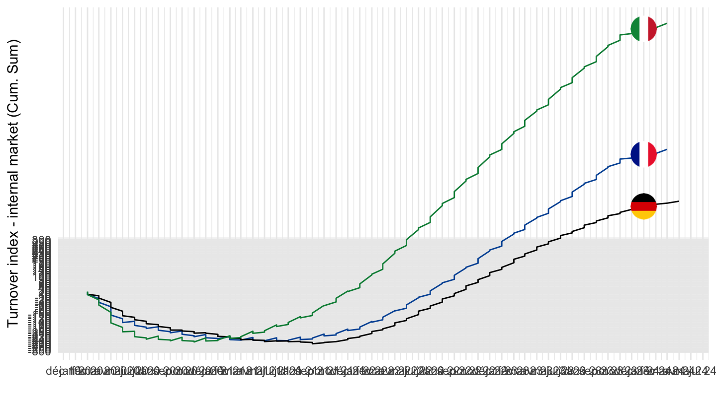
ei_isin_m %>%
  filter(nace_r2 == "C",
         indic == "IS-ITD",
         geo %in% c("FR", "DE", "IT", "ES"),
         s_adj == "SCA") %>%
  select(geo, time, values) %>%
  group_by(geo) %>%
  mutate(values = 100*values/values[time == "2020M02"]) %>%
  left_join(geo, by = "geo") %>%
  month_to_date %>%
  filter(date >= as.Date("2020-02-01")) %>%
  group_by(Geo) %>%
  arrange(date) %>%
  mutate(values = values-100,
         values = cumsum(values)) %>%
  ggplot() + ylab("Turnover index - internal market (Cum. Sum)") + xlab("") + theme_minimal() +
  geom_line(aes(x = date, y = values, color = Geo)) +
  scale_color_manual(values = c("#0055a4", "#000000", "#008c45", "#C60B1E")) +
  scale_x_date(breaks = "1 month",
               labels = date_format("%b %y")) + add_4flags +
  theme(legend.position = "none") +
  scale_y_continuous(breaks = seq(-300, 300, 10))