
Last observation: Q2 2026 (N = 3087)
First observation: Q1 1980 (N = 72)
Last data update: 23 oct. 2026, 00:25
Last compile: 25 oct. 2026, 23:13
namq_10_pc |>
  filter(geo %in% c("FR", "DE", "IT", "ES", "NL"),
         na_item == "B1GQ",
         unit == "CP_EUR_HAB") |>
  quarter_to_date() |>

  add_flag_color("Geo") |>
  ggplot() + geom_line(aes(x = date, y = values, color = color)) +
  theme_minimal() + scale_color_identity() + add_flags +
  scale_x_date(breaks = as.Date(paste0(seq(1980, 2100, 5), "-01-01")),
               labels = date_format("%Y")) +
  xlab("") + ylab("GDP per capita, current prices (€)")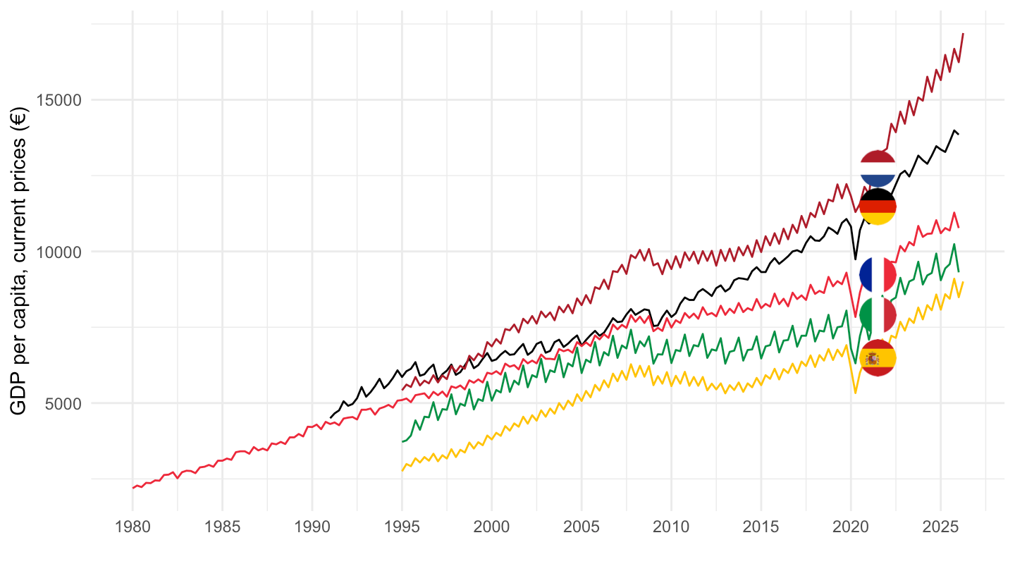
namq_10_pc |>
  filter(geo %in% c("FR", "DE", "IT", "ES", "NL"),
         na_item == "B1GQ",
         unit == "CLV_PCH_SM_HAB") |>
  quarter_to_date() |>

  add_flag_color("Geo") |>
  mutate(values = values/100) |>
  ggplot() + geom_line(aes(x = date, y = values, color = color)) +
  theme_minimal() + scale_color_identity() + add_flags +
  scale_x_date(breaks = as.Date(paste0(seq(1980, 2100, 5), "-01-01")),
               labels = date_format("%Y")) +
  xlab("") + ylab("GDP per capita, real growth (y-o-y)") +
  scale_y_continuous(labels = scales::percent_format(accuracy = 1)) +
  geom_hline(yintercept = 0, linetype = "dashed", color = "black")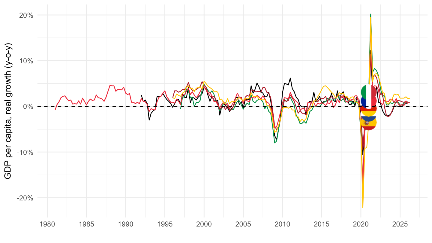
namq_10_pc |>
  filter(geo %in% c("FR", "DE", "IT", "ES", "EA20"),
         na_item == "B1GQ",
         # Chain linked volumes (2020), euro per capita; NSA only in this dataset
         unit == "CLV20_EUR_HAB") |>
  quarter_to_date() |>
  arrange(geo, date) |>
  group_by(geo) |>
  # 4-quarter moving average to remove seasonality (data are not seasonally adjusted)
  mutate(values = zoo::rollmeanr(values, 4, fill = NA)) |>
  filter(date >= as.Date("2017-10-01"), !is.na(values)) |>
  mutate(values = 100 * values / values[date == as.Date("2019-10-01")]) |>
  ungroup() |>
  mutate(Geo = ifelse(geo == "EA20", "Europe", Geo)) |>
  add_flag_color("Geo") |>
  ggplot() +
  # période Covid grisée
  annotate("rect", xmin = as.Date("2020-01-01"), xmax = as.Date("2021-12-31"),
           ymin = -Inf, ymax = Inf, fill = "grey60", alpha = 0.2) +
  annotate("text", x = as.Date("2021-01-01"), y = Inf, label = "Covid",
           vjust = 1.5, size = 3.5, color = "grey30") +
  geom_line(aes(x = date, y = values, color = color)) +
  theme_minimal() + scale_color_identity() + add_flags +
  scale_x_date(breaks = as.Date(paste0(seq(1980, 2100, 1), "-01-01")),
               labels = date_format("%Y")) +
  geom_hline(yintercept = 100, linetype = "dashed", color = "black") +
  xlab("") + ylab("PIB par habitant en volume\nmoyenne mobile sur 4 trimestres (base 100)")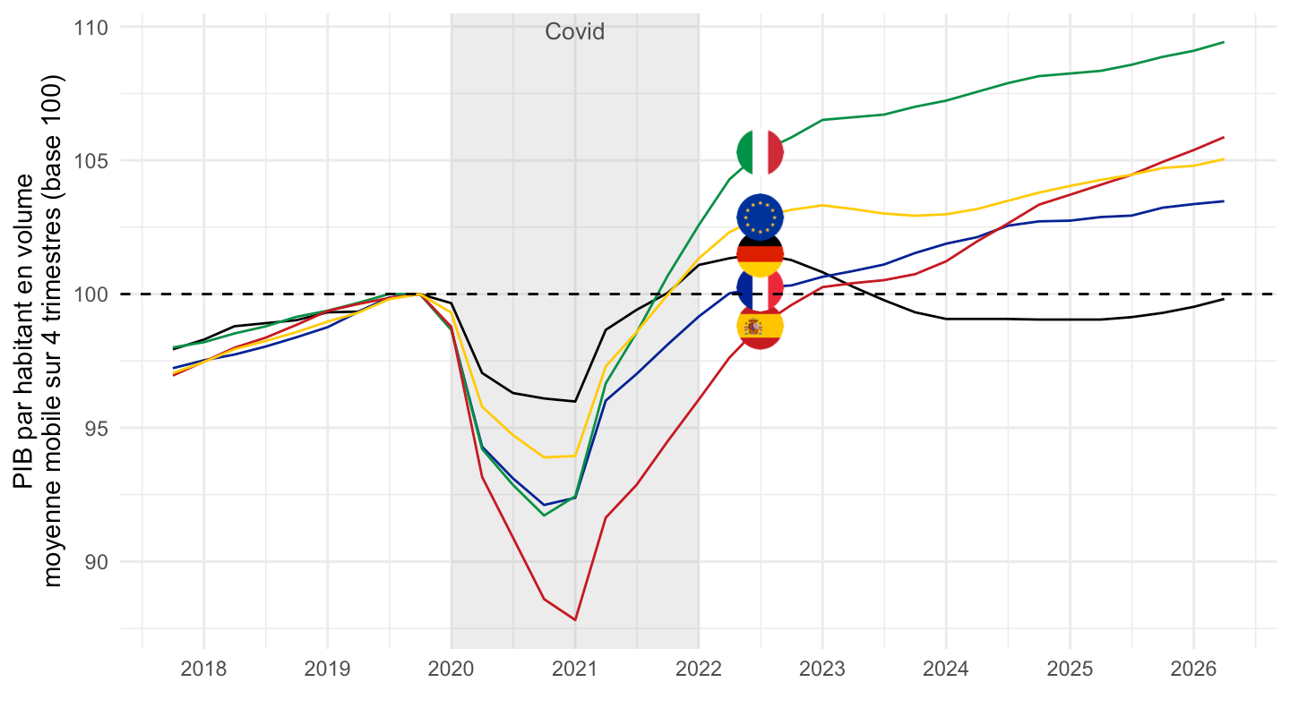
namq_10_pc |>
  filter(geo %in% c("FR", "DE", "IT", "ES", "EA20"),
         na_item == "B1GQ",
         # Chain linked volumes (2020), euro per capita; NSA only in this dataset
         unit == "CLV20_EUR_HAB") |>
  quarter_to_date() |>
  arrange(geo, date) |>
  group_by(geo) |>
  # 4-quarter moving average to remove seasonality (data are not seasonally adjusted)
  mutate(values = zoo::rollmeanr(values, 4, fill = NA)) |>
  filter(date >= as.Date("2007-10-01"), !is.na(values)) |>
  mutate(values = 100 * values / values[date == as.Date("2007-10-01")]) |>
  ungroup() |>
  mutate(Geo = ifelse(geo == "EA20", "Europe", Geo)) |>
  add_flag_color("Geo") |>
  ggplot() +
  # période Covid grisée
  annotate("rect", xmin = as.Date("2020-01-01"), xmax = as.Date("2021-12-31"),
           ymin = -Inf, ymax = Inf, fill = "grey60", alpha = 0.2) +
  annotate("text", x = as.Date("2021-01-01"), y = Inf, label = "Covid",
           vjust = 1.5, size = 3.5, color = "grey30") +
  geom_line(aes(x = date, y = values, color = color)) +
  theme_minimal() + scale_color_identity() + add_flags +
  scale_x_date(breaks = as.Date(paste0(seq(1980, 2100, 1), "-01-01")),
               labels = date_format("%Y")) +
  geom_hline(yintercept = 100, linetype = "dashed", color = "black") +
  xlab("") + ylab("PIB par habitant en volume\nmoyenne mobile sur 4 trimestres (base 100)")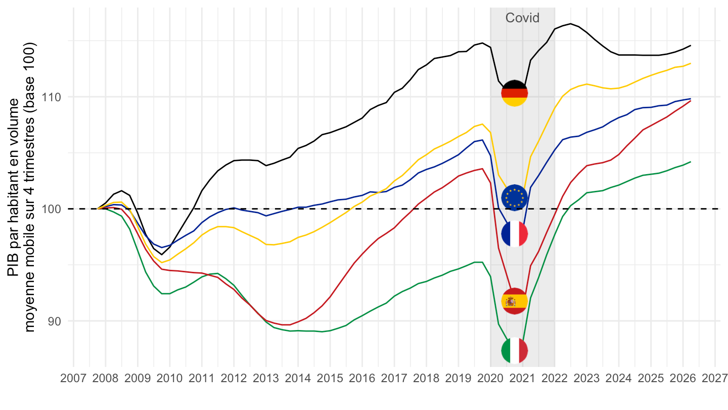
pays_fr <- c("DE" = "Allemagne", "EA20" = "Zone euro", "FR" = "France",
             "ES" = "Espagne", "IT" = "Italie")
d <- namq_10_pc |>
  filter(geo %in% names(pays_fr),
         na_item == "B1GQ",
         unit == "CLV20_EUR_HAB") |>
  quarter_to_date() |>
  arrange(geo, date) |>
  group_by(geo) |>
  mutate(values = zoo::rollmeanr(values, 4, fill = NA)) |>
  filter(date >= as.Date("2007-10-01"), !is.na(values)) |>
  mutate(values = 100 * values / values[date == as.Date("2007-10-01")]) |>
  ungroup() |>
  mutate(Geo = ifelse(geo == "EA20", "Europe", Geo)) |>
  add_flag_color("Geo") |>
  mutate(pays = factor(pays_fr[geo], levels = pays_fr))
pal <- d |> distinct(pays, color) |> tibble::deframe()
d |>
  ggplot(aes(x = date, y = values, color = pays)) +
  annotate("rect", xmin = as.Date("2020-01-01"), xmax = as.Date("2021-12-31"),
           ymin = -Inf, ymax = Inf, fill = "grey60", alpha = 0.2) +
  annotate("text", x = as.Date("2021-01-01"), y = Inf, label = "Covid",
           vjust = 1.5, size = 3.5, color = "grey30") +
  geom_hline(yintercept = 100, linewidth = 0.3, color = "grey40") +
  geom_line(linewidth = 0.6) +
  ggrepel::geom_text_repel(data = d |> slice_max(date, by = pays),
                           aes(label = pays), nudge_x = 250, hjust = 0,
                           direction = "y", segment.size = 0.3, min.segment.length = 0,
                           arrow = arrow(length = unit(0.015, "npc")),
                           size = 3.5, show.legend = FALSE) +
  theme_minimal() + xlab("") +
  ylab("PIB par habitant en volume\n(moy. mobile 4 trim., base 100 = T4 2007)") +
  scale_x_date(breaks = seq(as.Date("2008-01-01"), max(d$date), "2 years"),
               labels = scales::label_date("%Y"),
               expand = expansion(mult = c(0.01, 0.15))) +
  scale_y_continuous(breaks = seq(80, 130, 5)) +
  scale_color_manual(values = pal) +
  theme(legend.position = "none", panel.grid.minor = element_blank())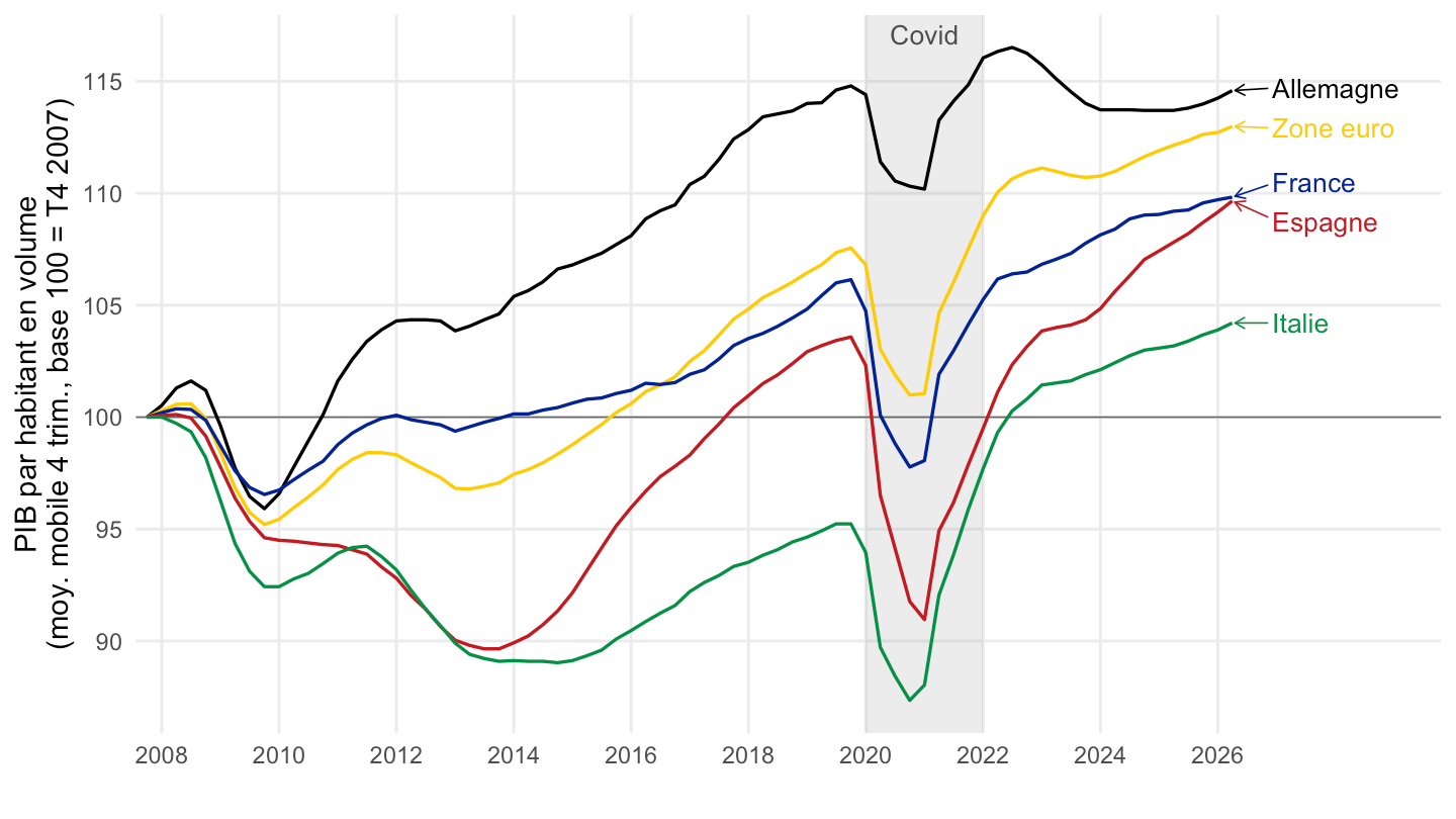
latest_q_pc <- namq_10_pc |>
  filter(na_item == "B1GQ",
         unit == "CP_EUR_HAB",
         geo %in% c("FR", "DE", "IT", "ES", "NL"),
         !is.na(values)) |>
  summarise(m = max(time)) |>
  pull(m)

namq_10_pc |>
  filter(na_item == "B1GQ",
         unit %in% c("CP_EUR_HAB", "CLV_PCH_SM_HAB"),
         geo %in% c("FR", "DE", "IT", "ES", "NL"),
         time == latest_q_pc) |>
  select(unit, Unit, Geo, values) |>
  spread(Geo, values) |>
print_table_conditional()| unit | Unit | France | Germany | Italy | Netherlands | Spain |
|---|---|---|---|---|---|---|
| CLV_PCH_SM_HAB | Chain linked volumes, percentage change compared to same period in previous year, per capita | 0.5 | 1.2 | 1.2 | 1.2 | 1.8 |
| CP_EUR_HAB | Current prices, euro per capita | 10970.0 | 13810.0 | 9700.0 | 17260.0 | 8990.0 |