National accounts employment data by industry (up to NACE A*64)
Data - Eurostat
Info
Last observation: Annual: 2025 (N = 10,058)
First observation: Annual: 1975 (N = 2,193)
Last data update: 23 jul 2026, 22:09. Last compile: 24 jul 2026, 02:38
Structure
Number of employees
Code
nama_10_a64_e %>%

  filter(geo %in% c("FR", "DE", "IT"),
         nace_r2 == "C",
         unit == "THS_HW",
         na_item == "EMP_DC") %>%
  year_to_date() %>%
  arrange(date) %>%
  ggplot(.) + geom_line(aes(x = date, y = values/1000, color = Geo)) +
  theme_minimal() + xlab("") + ylab("Number of Hours Worked") +
  geom_image(data = . %>%
               filter(date == as.Date("2010-01-01")) %>%
               mutate(image = paste0("../../icon/flag/round/", str_to_lower(Geo), ".png")),
             aes(x = date, y = values/1000, image = image), asp = 1.5) +
  scale_x_date(breaks = seq(1960, 2100, 5) %>% paste0("-01-01") %>% as.Date,
               labels = date_format("%Y")) +
  scale_y_continuous(breaks = seq(0, 1000000, 1000),
                     labels = dollar_format(accuracy = 1, prefix = "", suffix = "M")) +
  scale_color_manual(values = c("#0055a4", "#000000", "#008c45")) +
  theme(legend.position = c(0.2, 0.80),
        legend.title = element_blank())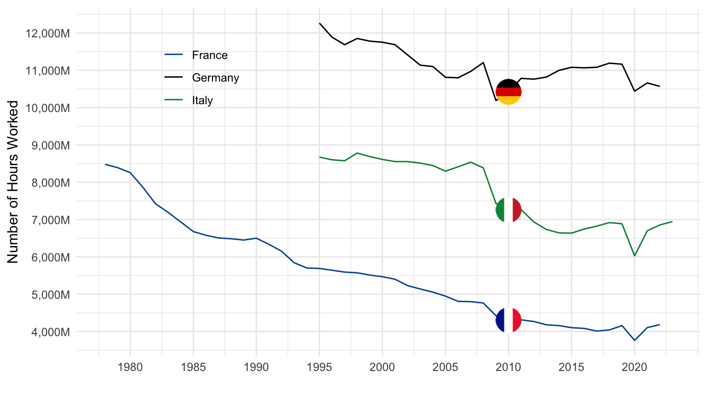
Number of hours worked
Code
nama_10_a64_e %>%

  filter(geo %in% c("FR", "DE", "IT"),
         nace_r2 == "TOTAL",
         unit == "THS_PER",
         na_item == "EMP_DC") %>%
  year_to_date() %>%
  arrange(date) %>%
  mutate(values = values/1000) %>%
  ggplot(.) + geom_line(aes(x = date, y = values, color = Geo)) +
  theme_minimal() + xlab("") + ylab("Number of Hours Worked") +
  add_3flags +
  scale_x_date(breaks = seq(1960, 2100, 5) %>% paste0("-01-01") %>% as.Date,
               labels = date_format("%Y")) +
  scale_color_manual(values = c("#0055a4", "#000000", "#008c45")) +
  theme(legend.position = c(0.2, 0.80),
        legend.title = element_blank())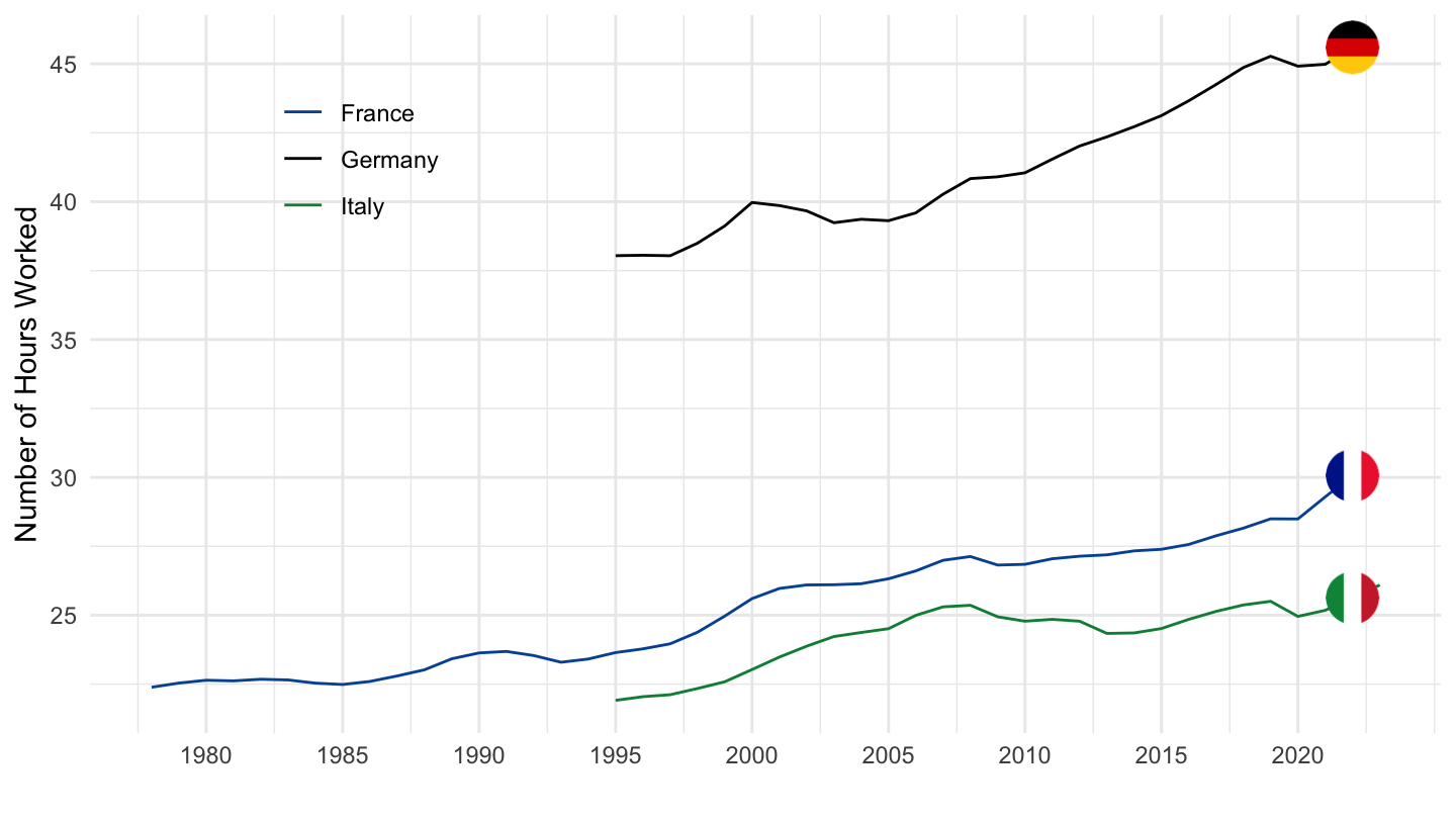
France VS Europe
Manufacture, Industrie
% de l’emploi
Code
nama_10_a64_e %>%
  filter(na_item == "EMP_DC",
         nace_r2 %in% c("C", "TOTAL", "B-E"),
         geo %in% c("FR", "EA19"),
         unit== "THS_PER") %>%
  year_to_date() %>%

  mutate(Geo = ifelse(geo == "EA19", "Europe", Geo)) %>%

  group_by(date) %>%
  mutate(values = values/ values[nace_r2 == "TOTAL"]) %>%
  filter(nace_r2 != "TOTAL",
         date >= as.Date("1995-01-01")) %>%
  mutate(Geo = ifelse(geo == "DE", "Germany", Geo)) %>%
  left_join(colors, by = c("Geo" = "country")) %>%
  ggplot(.) + geom_line(aes(x = date, y = values, color = color, linetype = Nace_r2)) +
  scale_color_identity() +
  scale_linetype_manual(values = c("solid", "dashed")) +
  theme_minimal() +
  scale_x_date(breaks = seq(1920, 2100, 5) %>% paste0("-01-01") %>% as.Date,
               labels = date_format("%Y")) +
  theme(legend.position = c(0.8, 0.9),
        legend.title = element_blank()) +
  add_4flags +
  scale_y_continuous(breaks = 0.01*seq(-60, 60, 2),
                     labels = scales::percent_format(accuracy = 1)) +
  ylab("Emploi Manufacturier, Industriel (% de l'Emploi)") + xlab("")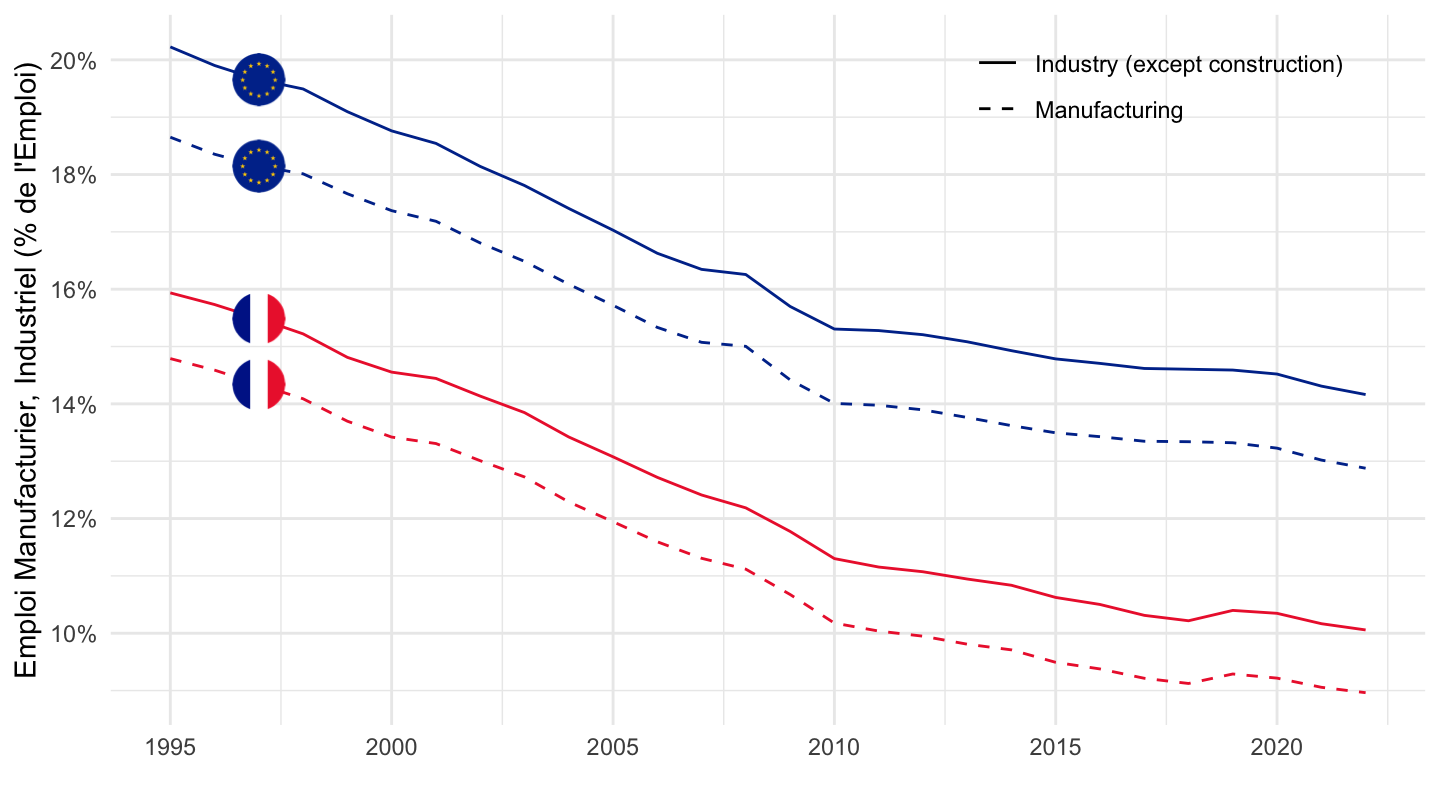
THS_PER, Nombre d’emplois
Code
nama_10_a64_e %>%
  filter(na_item == "EMP_DC",
         nace_r2 %in% c("C", "B-E"),
         geo %in% c("FR", "EA19", "DE"),
         unit== "THS_PER") %>%
  year_to_date() %>%

  mutate(Geo = ifelse(geo == "EA19", "Europe", Geo)) %>%

  #filter(date >= as.Date("1995-01-01")) %>%
  left_join(colors, by = c("Geo" = "country")) %>%
  ggplot(.) + geom_line(aes(x = date, y = values, color = color, linetype = Nace_r2)) +
  scale_color_identity() +
  scale_linetype_manual(values = c("solid", "dashed")) +
  theme_minimal() +
  scale_x_date(breaks = seq(1920, 2100, 5) %>% paste0("-01-01") %>% as.Date,
               labels = date_format("%Y")) +
  theme(legend.position = c(0.2, 0.9),
        legend.title = element_blank()) +
  add_6flags +
  scale_y_log10(breaks = 100*seq(0, 1000, 10)) +
  ylab("Emploi Manufacturier, Industriel (Milliers d'emplois)") + xlab("")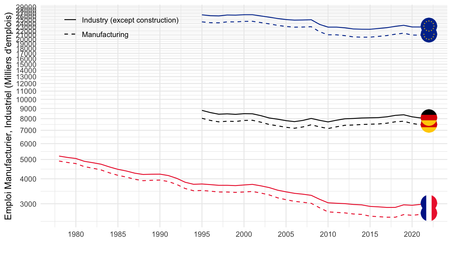
France VS Germany
Table
Code
load_data("eurostat/nace_r2_fr.RData")
nama_10_a64_e %>%
  filter(geo %in% c("FR", "DE"),
         unit == "THS_PER",
         na_item == "EMP_DC",
         time %in% c("2019")) %>%
  filter(!grepl("C", nace_r2) | nace_r2 == "TOTAL") %>%
  select(-na_item, -unit, -time) %>%


  select(nace_r2, Nace_r2, Geo, values) %>%
  group_by(Geo) %>%
  mutate(values = round(100*values/ values[nace_r2 == "TOTAL"], 1)) %>%
  filter(nace_r2 != "TOTAL")  %>%
  spread(Geo, values) %>%
  mutate(difference = `France` - `Germany`) %>%
  arrange(-difference) %>%
  {if (is_html_output()) datatable(., filter = 'top', rownames = F, escape = F) else .}
Table 1995, 2019
Code
load_data("eurostat/nace_r2_fr.RData")
nama_10_a64_e %>%
  filter(geo %in% c("FR", "DE"),
         unit == "THS_PER",
         na_item == "EMP_DC",
         time %in% c("1995", "2019")) %>%


  select(-na_item, -unit) %>%
  transmute(nace_r2, Nace_r2, variable = paste(Geo, time), values) %>%
  group_by(variable) %>%
  mutate(values = round(100*values/ values[nace_r2 == "TOTAL"], 1)) %>%
  filter(nace_r2 != "TOTAL")  %>%
  spread(variable, values) %>%
  mutate(difference = `France 2019` - `France 1995` - (`Germany 2019` - `Germany 1995`)) %>%
  arrange(-abs(difference)) %>%
  {if (is_html_output()) datatable(., filter = 'top', rownames = F, escape = F) else .}
Manufacture, Industrie
% de l’emploi
Code
nama_10_a64_e %>%
  filter(na_item == "EMP_DC",
         nace_r2 %in% c("C", "TOTAL", "B-E"),
         geo %in% c("FR", "DE"),
         unit== "THS_PER") %>%
  year_to_date() %>%


  group_by(date) %>%
  mutate(values = values/ values[nace_r2 == "TOTAL"]) %>%
  filter(nace_r2 != "TOTAL",
         date >= as.Date("1995-01-01")) %>%
  mutate(Geo = ifelse(geo == "DE", "Germany", Geo)) %>%
  left_join(colors, by = c("Geo" = "country")) %>%
  ggplot(.) + geom_line(aes(x = date, y = values, color = color, linetype = Nace_r2)) +
  scale_color_identity() +
  scale_linetype_manual(values = c("solid", "dashed")) +
  theme_minimal() +
  scale_x_date(breaks = seq(1920, 2100, 5) %>% paste0("-01-01") %>% as.Date,
               labels = date_format("%Y")) +
  theme(legend.position = c(0.8, 0.9),
        legend.title = element_blank()) +
  add_4flags +
  scale_y_continuous(breaks = 0.01*seq(-60, 60, 2),
                     labels = scales::percent_format(accuracy = 1)) +
  ylab("Emploi Manufacturier, Industriel (% de l'Emploi)") + xlab("")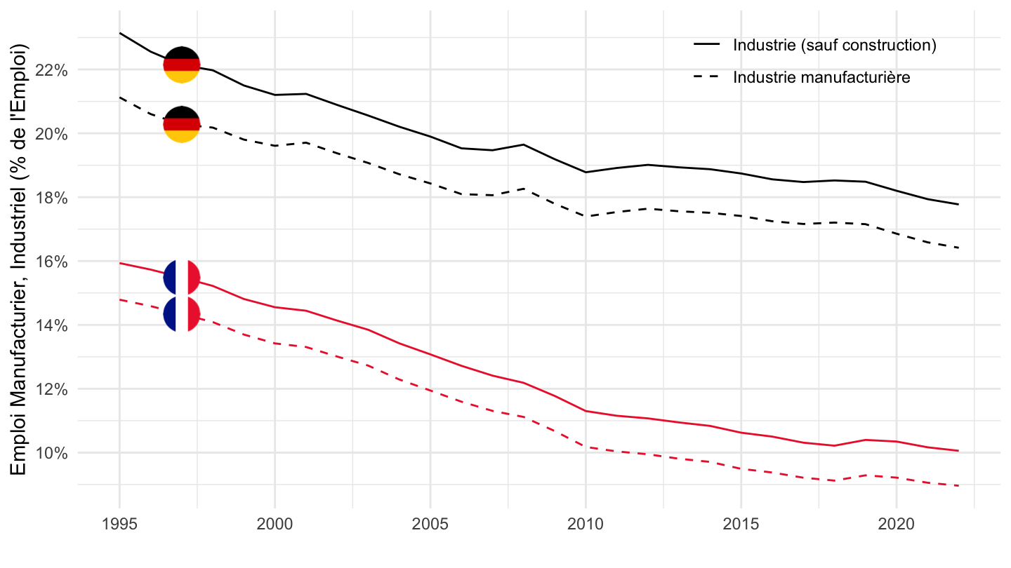
% des heures (THS_HW)
Code
nama_10_a64_e %>%
  filter(na_item == "EMP_DC",
         nace_r2 %in% c("C", "TOTAL", "B-E"),
         geo %in% c("FR", "DE"),
         unit== "THS_HW") %>%
  year_to_date() %>%


  group_by(date) %>%
  mutate(values = values/ values[nace_r2 == "TOTAL"]) %>%
  filter(nace_r2 != "TOTAL",
         date >= as.Date("1995-01-01")) %>%
  mutate(Geo = ifelse(geo == "DE", "Germany", Geo)) %>%
  left_join(colors, by = c("Geo" = "country")) %>%
  ggplot(.) + geom_line(aes(x = date, y = values, color = color, linetype = Nace_r2)) +
  scale_color_identity() +
  scale_linetype_manual(values = c("solid", "dashed")) +
  theme_minimal() +
  scale_x_date(breaks = seq(1920, 2100, 5) %>% paste0("-01-01") %>% as.Date,
               labels = date_format("%Y")) +
  theme(legend.position = c(0.8, 0.9),
        legend.title = element_blank()) +
  add_4flags +
  scale_y_continuous(breaks = 0.01*seq(-60, 60, 2),
                     labels = scales::percent_format(accuracy = 1)) +
  ylab("Emploi Manufacturier, Industriel (% des heures)") + xlab("")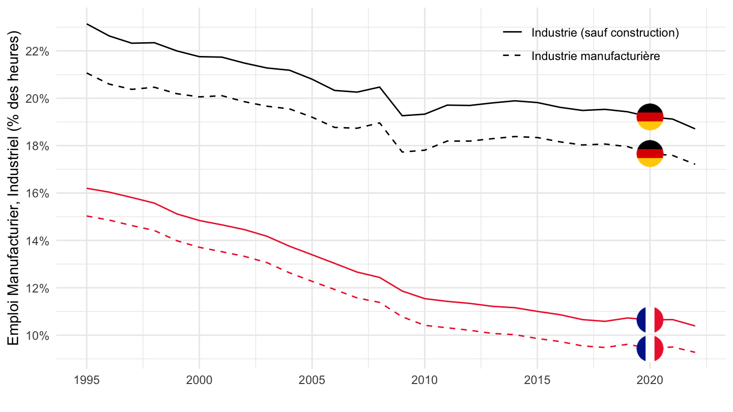
THS_PER, Nombre d’emplois
Code
nama_10_a64_e %>%
  filter(na_item == "EMP_DC",
         nace_r2 %in% c("C", "B-E"),
         geo %in% c("FR", "DE"),
         unit== "THS_PER") %>%
  year_to_date() %>%


  #filter(date >= as.Date("1995-01-01")) %>%
  mutate(Geo = ifelse(geo == "DE", "Germany", Geo)) %>%
  left_join(colors, by = c("Geo" = "country")) %>%
  ggplot(.) + geom_line(aes(x = date, y = values, color = color, linetype = Nace_r2)) +
  scale_color_identity() +
  scale_linetype_manual(values = c("solid", "dashed")) +
  theme_minimal() +
  scale_x_date(breaks = seq(1920, 2100, 5) %>% paste0("-01-01") %>% as.Date,
               labels = date_format("%Y")) +
  theme(legend.position = c(0.2, 0.9),
        legend.title = element_blank()) +
  add_4flags +
  scale_y_continuous(breaks = 100*seq(0, 1000, 10)) +
  ylab("Emploi Manufacturier, Industriel (Milliers d'emplois)") + xlab("")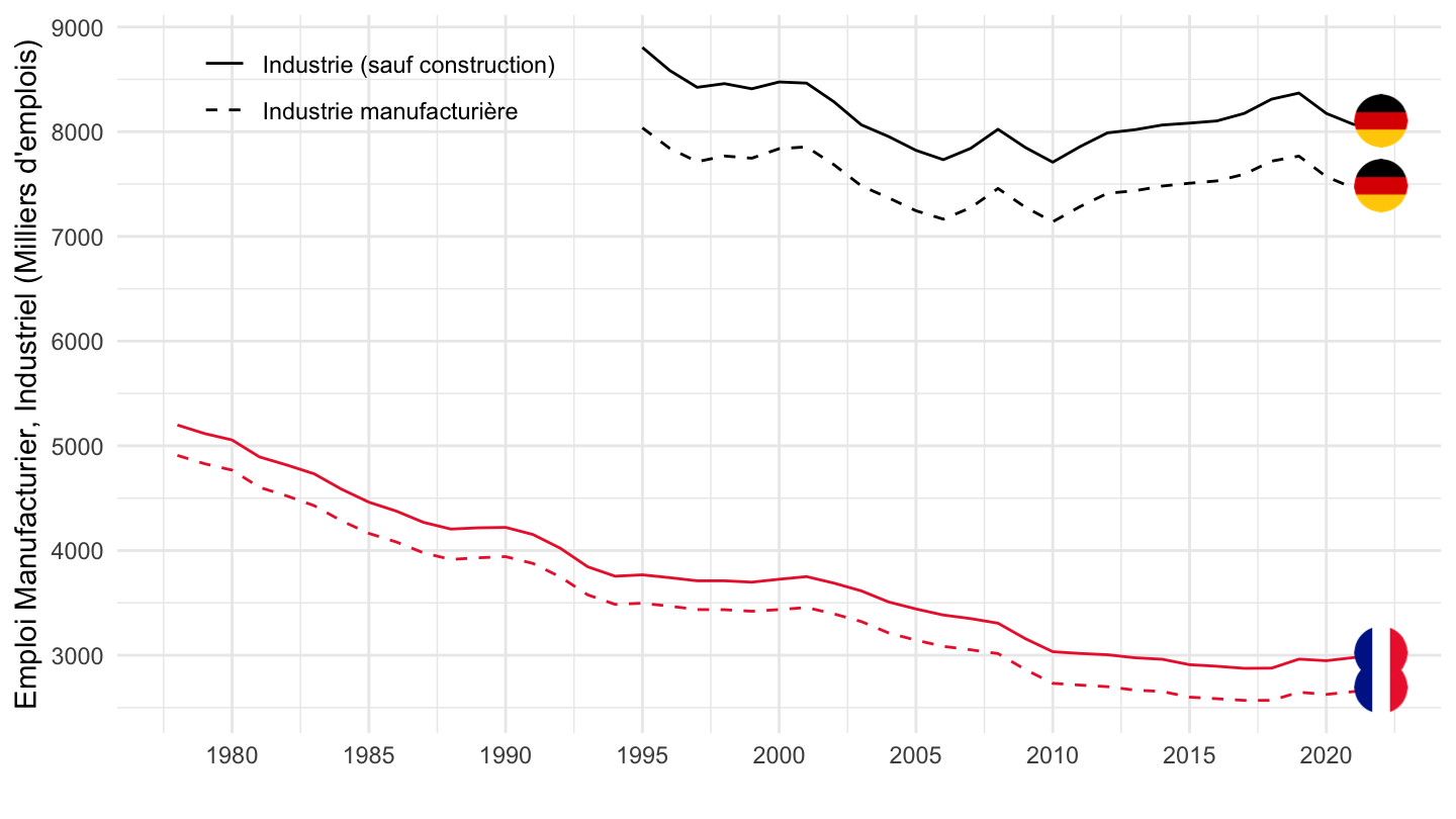
Manufacture, Administration
Code
nama_10_a64_e %>%
  filter(na_item == "EMP_DC",
         nace_r2 %in% c("O-Q", "TOTAL", "B-E"),
         geo %in% c("FR", "DE"),
         unit== "THS_HW") %>%
  year_to_date() %>%

  group_by(date) %>%
  mutate(values = values/ values[nace_r2 == "TOTAL"]) %>%
  filter(nace_r2 != "TOTAL",
         date >= as.Date("1995-01-01")) %>%
  mutate(Geo = ifelse(geo == "DE", "Germany", Geo)) %>%
  ggplot(.) + geom_line(aes(x = date, y = values, color = Geo, linetype = nace_r2)) +
  scale_color_manual(values = c("#0055a4", "#000000")) +
  scale_linetype_manual(values = c("solid", "dashed")) +
  theme_minimal() +
  scale_x_date(breaks = seq(1920, 2100, 5) %>% paste0("-01-01") %>% as.Date,
               labels = date_format("%Y")) +
  theme(legend.position = "none") +
  add_4flags +
  scale_y_continuous(breaks = 0.01*seq(-60, 60, 2),
                     labels = scales::percent_format(accuracy = 1)) +
  ylab("Emploi Manufacturier, Industriel (% de l'Emploi)") + xlab("")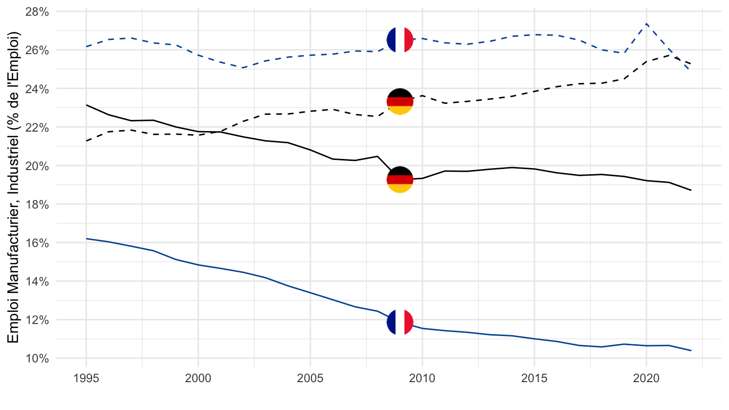
G, C, F
Code
nama_10_a64_e %>%
  filter(na_item == "EMP_DC",
         nace_r2 %in% c("G", "C", "F","TOTAL"),
         geo %in% c("FR", "DE"),
         unit== "THS_HW") %>%
  year_to_date() %>%


  group_by(date) %>%
  mutate(values = values/ values[nace_r2 == "TOTAL"]) %>%
  filter(nace_r2 != "TOTAL",
         date >= as.Date("1995-01-01")) %>%
  ggplot(.) + geom_line(aes(x = date, y = values, color = Geo, linetype = Nace_r2)) +
  scale_color_manual(values = c("#0055a4", "#000000")) +
  scale_linetype_manual(values = c("solid", "dashed", "longdash")) +
  theme_minimal() +
  scale_x_date(breaks = seq(1920, 2100, 5) %>% paste0("-01-01") %>% as.Date,
               labels = date_format("%Y")) +
  theme(legend.position = c(0.4, 0.5)) +
  add_6flags +
  scale_y_continuous(breaks = 0.01*seq(-60, 60, 2),
                     labels = scales::percent_format(accuracy = 1)) +
  ylab("") + xlab("")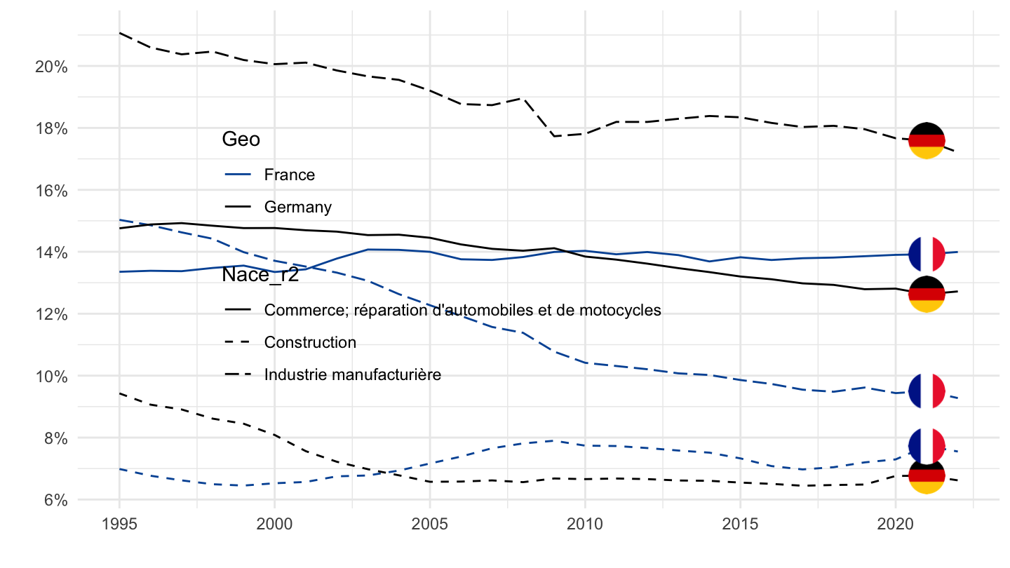
P, M, K
Code
nama_10_a64_e %>%
  filter(na_item == "EMP_DC",
         nace_r2 %in% c("P", "M", "K","TOTAL"),
         geo %in% c("FR", "DE"),
         unit== "THS_HW") %>%
  year_to_date() %>%


  group_by(date) %>%
  mutate(values = values/ values[nace_r2 == "TOTAL"]) %>%
  filter(nace_r2 != "TOTAL",
         date >= as.Date("1995-01-01")) %>%
  ggplot(.) + geom_line(aes(x = date, y = values, color = Geo, linetype = Nace_r2)) +
  scale_color_manual(values = c("#0055a4", "#000000")) +
  scale_linetype_manual(values = c("solid", "dashed", "longdash")) +
  theme_minimal() +
  scale_x_date(breaks = seq(1920, 2100, 5) %>% paste0("-01-01") %>% as.Date,
               labels = date_format("%Y")) +
  theme(legend.position = c(0.3, 0.7)) +
  add_6flags +
  scale_y_continuous(breaks = 0.01*seq(-60, 60, 1),
                     labels = scales::percent_format(accuracy = 1)) +
  ylab("Emploi Manufacturier, Industriel (% de l'Emploi)") + xlab("")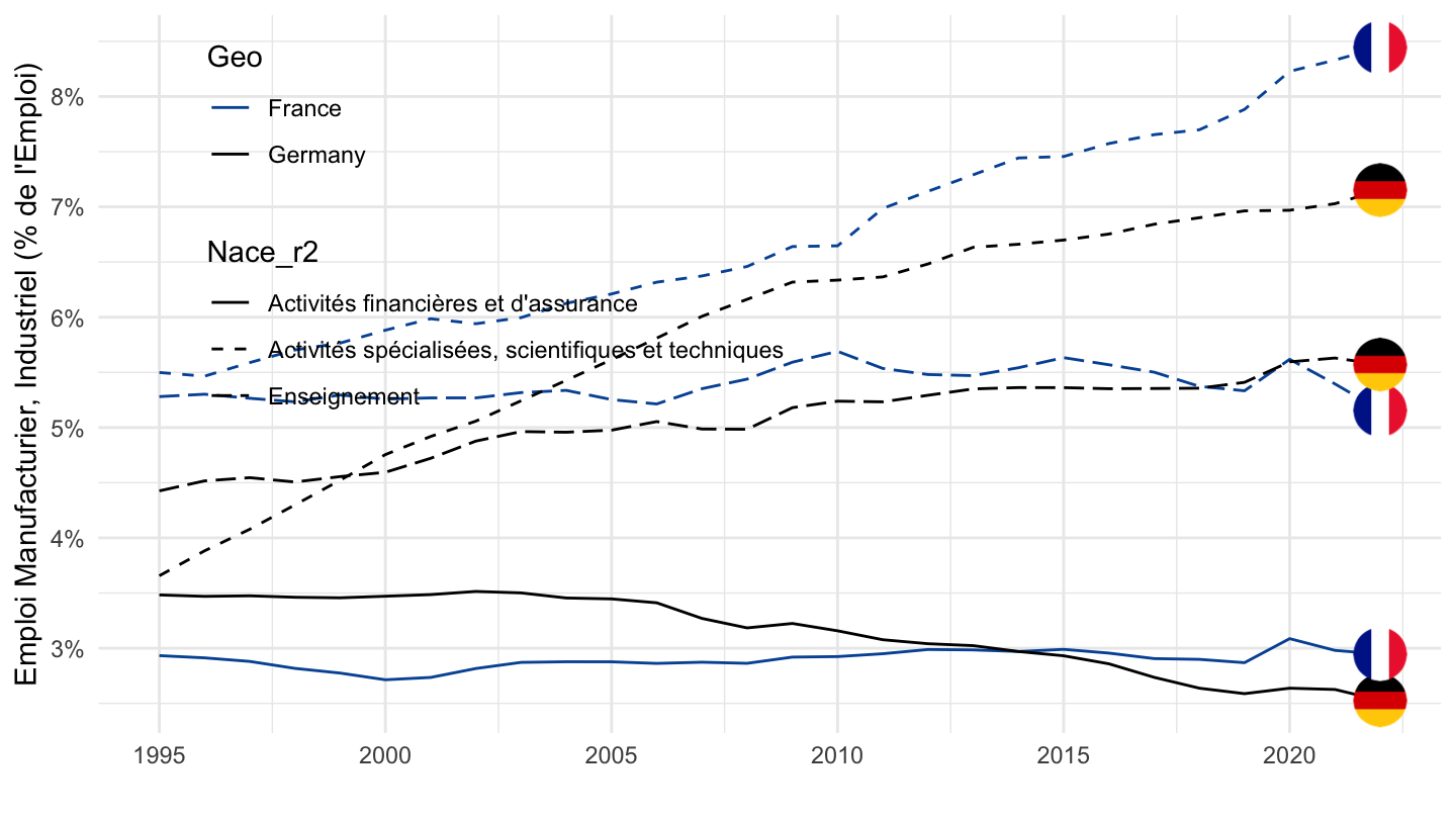
Germany, Italy, France, Spain
Table - Flags
Code
load_data("eurostat/nace_r2_fr.RData")
nama_10_a64_e %>%
  filter(geo %in% c("FR", "DE", "IT", "ES"),
         unit == "THS_PER",
         na_item == "EMP_DC",
         time %in% c("2018")) %>%
  filter(!grepl("C", nace_r2) | nace_r2 == "TOTAL") %>%
  select(-na_item, -unit, -time) %>%


  mutate(Flag = gsub(" ", "-", str_to_lower(Geo)),
         Flag = paste0('<img src="../../bib/flags/vsmall/', Flag, '.png" alt="Flag">')) %>%
  select(nace_r2, Nace_r2, Flag, values) %>%
  group_by(Flag) %>%
  mutate(values = round(100*values/ values[nace_r2 == "TOTAL"], 1)) %>%
  filter(nace_r2 != "TOTAL")  %>%
  spread(Flag, values) %>%
  {if (is_html_output()) datatable(., filter = 'top', rownames = F, escape = F) else .}
Table - Manufacturing
Code
load_data("eurostat/nace_r2_fr.RData")
nama_10_a64_e %>%
  filter(geo %in% c("FR", "DE", "IT", "ES"),
         unit == "THS_PER",
         na_item == "EMP_DC",
         time %in% c("2018")) %>%
  filter(grepl("C", nace_r2) | nace_r2 == "TOTAL") %>%
  select(-na_item, -unit, -time) %>%


  mutate(Flag = gsub(" ", "-", str_to_lower(Geo)),
         Flag = paste0('<img src="../../bib/flags/vsmall/', Flag, '.png" alt="Flag">')) %>%
  select(nace_r2, Nace_r2, Flag, values) %>%
  group_by(Flag) %>%
  mutate(values = round(100*values/ values[nace_r2 == "TOTAL"], 1)) %>%
  filter(nace_r2 != "TOTAL")  %>%
  spread(Flag, values) %>%
  {if (is_html_output()) datatable(., filter = 'top', rownames = F, escape = F) else .}
C - Manufacturing
Value
Code
nama_10_a64_e %>%
  filter(unit == "THS_PER",
         na_item == "EMP_DC",
         nace_r2 %in% c("C", "TOTAL"),
         geo %in% c("FR", "DE", "IT", "ES")) %>%
  year_to_date() %>%

  select(geo,  Geo, nace_r2, date, values) %>%
  spread(nace_r2, values) %>%
  mutate(values = `C`/TOTAL) %>%
  left_join(colors, by = c("Geo" = "country")) %>%
  ggplot(.) + geom_line(aes(x = date, y = values, color = color)) +
  theme_minimal() + xlab("") + ylab("Manufacturing (% of GDP)") +
  scale_color_identity() + add_4flags +
  scale_x_date(breaks = seq(1960, 2100, 5) %>% paste0("-01-01") %>% as.Date,
               labels = date_format("%Y")) +
  scale_y_continuous(breaks = 0.01*seq(-500, 200, 1),
                     labels = percent_format(accuracy = 1))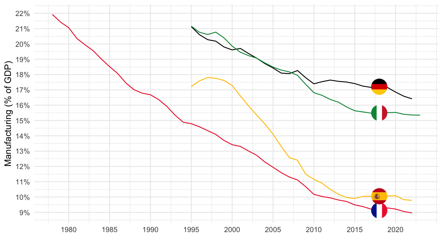
Productivity
Normal
Code
nama_10_a64 %>%
  filter(na_item == "B1G",
         nace_r2 %in% c("C"),
         geo %in% c("FR", "DE", "IT", "ES", "NL"),
         unit %in% c("CP_MNAC", "CLV10_MEUR")) %>%
  select_if(~ n_distinct(.) > 1) %>%
  rename(B1G = values) %>%
  left_join(nama_10_a64_e %>%
              filter(nace_r2 %in% c("C"),
                     geo %in% c("FR", "DE", "IT", "ES", "NL"),
                     unit == "THS_PER",
                     na_item == "EMP_DC") %>%
              select_if(~ n_distinct(.) > 1) %>%
              rename(EMP_DC = values), by = c("geo", "time", "Geo")) %>%
  mutate(values = B1G/EMP_DC) %>%
  year_to_date() %>%
  filter(date >= as.Date("1995-01-01")) %>%


  left_join(colors, by = c("Geo" = "country")) %>%
  mutate(color = ifelse(geo == "NL", color2, color)) %>%
  ggplot(.) + geom_line(aes(x = date, y = values, color = color, linetype = Unit)) +
  theme_minimal() + xlab("") + ylab("C - Manufacturing\n Labour Productivity = B1G / EMP_DC") +
  scale_color_identity() + add_flags +
  scale_x_date(breaks = seq(1960, 2100, 5) %>% paste0("-01-01") %>% as.Date,
               labels = date_format("%Y")) +
  theme(legend.position = c(0.3, 0.8)) +
  scale_y_continuous(breaks = seq(0, 2000, 10),
                     labels = dollar_format(pre = "", su = "k€", acc = 1))
Log
Code
nama_10_a64 %>%
  filter(na_item == "B1G",
         nace_r2 %in% c("C"),
         geo %in% c("FR", "DE", "IT", "ES", "NL"),
         unit %in% c("CP_MNAC", "CLV10_MEUR")) %>%
  select_if(~ n_distinct(.) > 1) %>%
  rename(B1G = values) %>%
  left_join(nama_10_a64_e %>%
              filter(nace_r2 %in% c("C"),
                     geo %in% c("FR", "DE", "IT", "ES", "NL"),
                     unit == "THS_PER",
                     na_item == "EMP_DC") %>%
              select_if(~ n_distinct(.) > 1) %>%
              rename(EMP_DC = values), by = c("geo", "Geo", "time")) %>%
  mutate(values = B1G/EMP_DC) %>%
  year_to_date() %>%
  filter(date >= as.Date("1995-01-01")) %>%


  left_join(colors, by = c("Geo" = "country")) %>%
  mutate(color = ifelse(geo == "NL", color2, color)) %>%
  ggplot(.) + geom_line(aes(x = date, y = values, color = color, linetype = Unit)) +
  theme_minimal() + xlab("") + ylab("C - Manufacturing\n Labour Productivity = B1G / EMP_DC") +
  scale_color_identity() + add_flags +
  scale_x_date(breaks = seq(1960, 2100, 5) %>% paste0("-01-01") %>% as.Date,
               labels = date_format("%Y")) +
  theme(legend.position = c(0.3, 0.8)) +
  scale_y_log10(breaks = seq(0, 2000, 50),
                     labels = dollar_format(pre = "", su = "k€", acc = 1))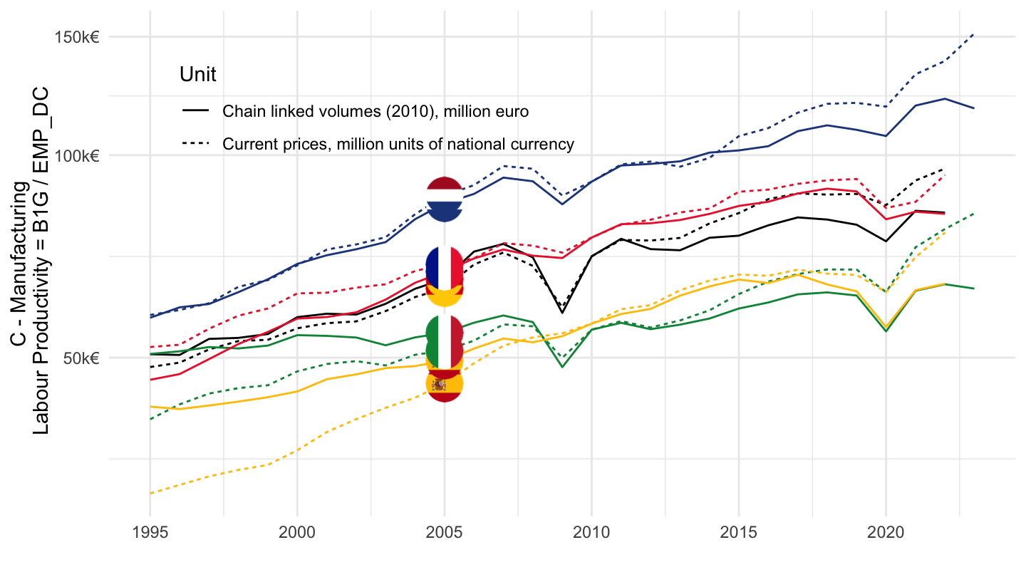
Base 100
Code
nama_10_a64 %>%
  filter(na_item == "B1G",
         nace_r2 %in% c("C"),
         geo %in% c("FR", "DE", "IT", "ES", "NL"),
         unit %in% c("CP_MNAC", "CLV10_MEUR")) %>%
  select_if(~ n_distinct(.) > 1) %>%
  rename(B1G = values) %>%
  left_join(nama_10_a64_e %>%
              filter(nace_r2 %in% c("C"),
                     geo %in% c("FR", "DE", "IT", "ES", "NL"),
                     unit == "THS_PER",
                     na_item == "EMP_DC") %>%
              select_if(~ n_distinct(.) > 1) %>%
              rename(EMP_DC = values), by = c("geo", "Geo", "time")) %>%
  mutate(values = B1G/EMP_DC) %>%
  year_to_date() %>%
  filter(date >= as.Date("1995-01-01")) %>%


  left_join(colors, by = c("Geo" = "country")) %>%
  mutate(color = ifelse(geo == "NL", color2, color)) %>%
  group_by(Geo, Unit) %>%
  arrange(date) %>%
  mutate(values = 100*values/values[1]) %>%
  ggplot(.) + geom_line(aes(x = date, y = values, color = color, linetype = Unit)) +
  theme_minimal() + xlab("") + ylab("C - Manufacturing\n Labour Productivity = B1G / EMP_DC") +
  scale_color_identity() + add_flags +
  scale_x_date(breaks = seq(1960, 2100, 5) %>% paste0("-01-01") %>% as.Date,
               labels = date_format("%Y")) +
  theme(legend.position = c(0.3, 0.8)) +
  scale_y_log10(breaks = seq(0, 2000, 20))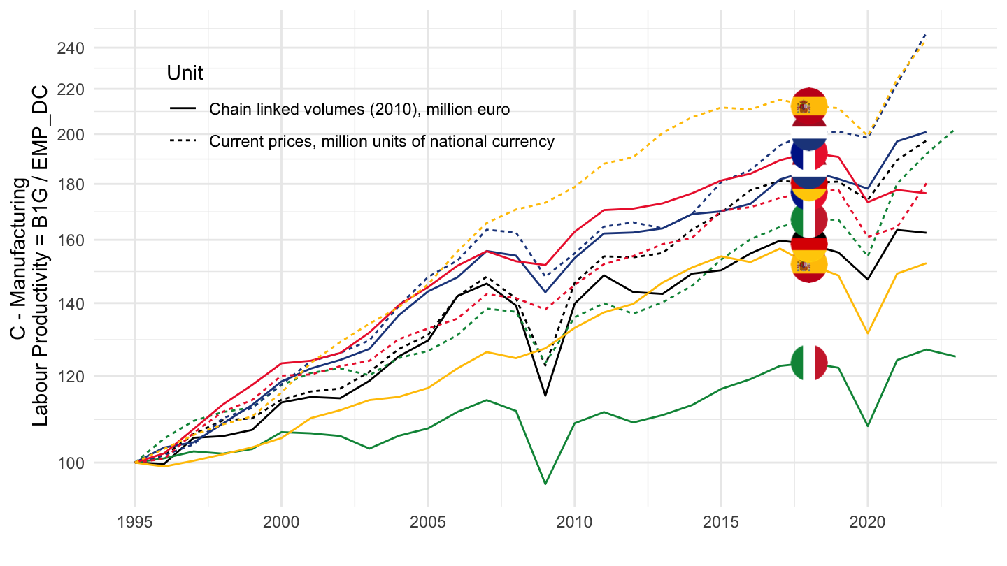
C10-C12 - Food products
Value
All
Code
nama_10_a64_e %>%
  filter(nace_r2 %in% c("C10-C12", "TOTAL"),
         geo %in% c("FR", "DE", "IT", "ES"),
         unit == "THS_PER",
         na_item == "EMP_DC") %>%
  year_to_date() %>%

  select(geo,  Geo, nace_r2, date, values) %>%
  spread(nace_r2, values) %>%
  mutate(values = `C10-C12`/TOTAL) %>%
  left_join(colors, by = c("Geo" = "country")) %>%
  ggplot(.) + geom_line(aes(x = date, y = values, color = color)) +
  theme_minimal() + xlab("") + ylab("Food products (% of GDP)") +
  scale_color_identity() + add_4flags +
  scale_x_date(breaks = seq(1960, 2100, 5) %>% paste0("-01-01") %>% as.Date,
               labels = date_format("%Y")) +
  scale_y_continuous(breaks = 0.01*seq(-500, 200, 0.1),
                     labels = percent_format(accuracy = .1))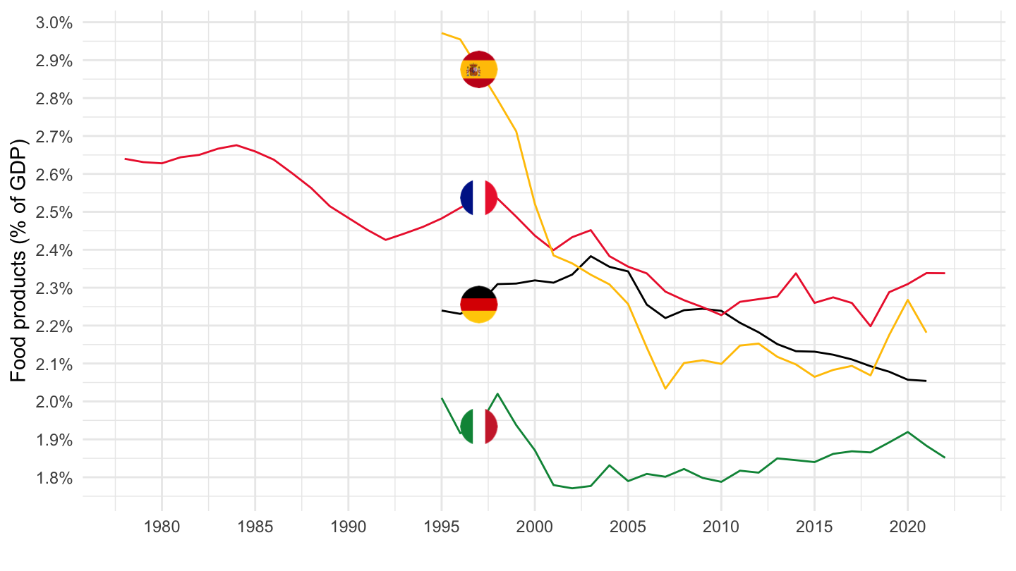
1995-
Code
nama_10_a64_e %>%
  filter(nace_r2 %in% c("C10-C12", "TOTAL"),
         geo %in% c("FR", "DE", "IT", "ES"),
         unit == "THS_PER",
         na_item == "EMP_DC") %>%
  year_to_date() %>%
  filter(date >= as.Date("1995-01-01")) %>%

  select(geo,  Geo, nace_r2, date, values) %>%
  spread(nace_r2, values) %>%
  ggplot(.) + geom_line(aes(x = date, y = `C10-C12`/TOTAL, color = Geo)) +
  theme_minimal() + xlab("") + ylab("Food products (% of GDP)") +
  scale_color_manual(values = c("#002395", "#000000", "#009246", "#C60B1E")) +
  scale_x_date(breaks = seq(1960, 2100, 2) %>% paste0("-01-01") %>% as.Date,
               labels = date_format("%Y")) +
  geom_image(data = . %>%
               filter(date == as.Date("2015-01-01")) %>%
               mutate(image = paste0("../../icon/flag/round/", str_to_lower(Geo), ".png")),
             aes(x = date, y = `C10-C12`/TOTAL, image = image), asp = 1.5) +
  theme(legend.position = "none") +
  scale_y_continuous(breaks = 0.01*seq(-500, 200, 0.1),
                     labels = percent_format(accuracy = .1))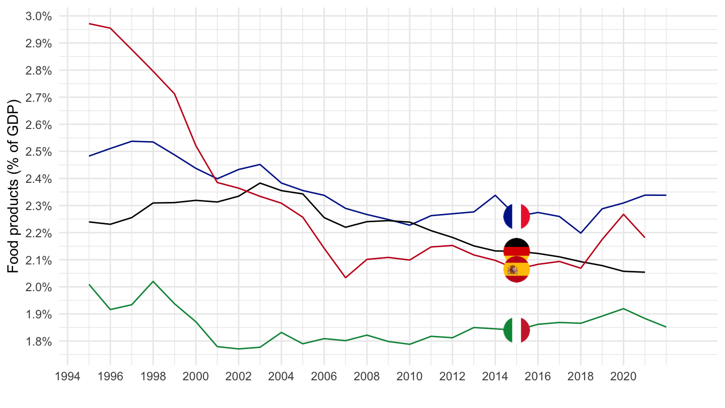
Productivity
Normal
Code
nama_10_a64 %>%
  filter(na_item == "B1G",
         nace_r2 %in% c("C10-C12"),
         geo %in% c("FR", "DE", "IT", "ES", "NL"),
         unit %in% c("CP_MNAC", "CLV10_MEUR")) %>%
  select_if(~ n_distinct(.) > 1) %>%
  rename(B1G = values) %>%
  left_join(nama_10_a64_e %>%
              filter(nace_r2 %in% c("C10-C12"),
                     geo %in% c("FR", "DE", "IT", "ES", "NL"),
                     unit == "THS_PER",
                     na_item == "EMP_DC") %>%
              select_if(~ n_distinct(.) > 1) %>%
              rename(EMP_DC = values), by = c("geo", "Geo", "time")) %>%
  mutate(values = B1G/EMP_DC) %>%
  year_to_date() %>%
  filter(date >= as.Date("1995-01-01")) %>%


  left_join(colors, by = c("Geo" = "country")) %>%
  mutate(color = ifelse(geo == "NL", color2, color)) %>%
  ggplot(.) + geom_line(aes(x = date, y = values, color = color, linetype = Unit)) +
  theme_minimal() + xlab("") + ylab("Labour Productivity = B1G / EMP_DC") +
  scale_color_identity() + add_flags +
  scale_x_date(breaks = seq(1960, 2100, 5) %>% paste0("-01-01") %>% as.Date,
               labels = date_format("%Y")) +
  theme(legend.position = c(0.3, 0.8)) +
  scale_y_continuous(breaks = seq(0, 2000, 50),
                     labels = dollar_format(pre = "", su = "k€", acc = 1))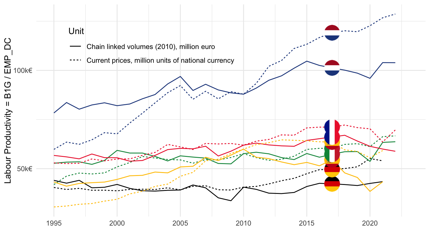
Log
Code
nama_10_a64 %>%
  filter(na_item == "B1G",
         nace_r2 %in% c("C10-C12"),
         geo %in% c("FR", "DE", "IT", "ES", "NL"),
         unit %in% c("CP_MNAC", "CLV10_MEUR")) %>%
  select_if(~ n_distinct(.) > 1) %>%
  rename(B1G = values) %>%
  left_join(nama_10_a64_e %>%
              filter(nace_r2 %in% c("C10-C12"),
                     geo %in% c("FR", "DE", "IT", "ES", "NL"),
                     unit == "THS_PER",
                     na_item == "EMP_DC") %>%
              select_if(~ n_distinct(.) > 1) %>%
              rename(EMP_DC = values), by = c("geo", "Geo", "time")) %>%
  mutate(values = B1G/EMP_DC) %>%
  year_to_date() %>%
  filter(date >= as.Date("1995-01-01")) %>%


  left_join(colors, by = c("Geo" = "country")) %>%
  mutate(color = ifelse(geo == "NL", color2, color)) %>%
  ggplot(.) + geom_line(aes(x = date, y = values, color = color, linetype = Unit)) +
  theme_minimal() + xlab("") + ylab("Labour Productivity = B1G / EMP_DC") +
  scale_color_identity() + add_flags +
  scale_x_date(breaks = seq(1960, 2100, 5) %>% paste0("-01-01") %>% as.Date,
               labels = date_format("%Y")) +
  theme(legend.position = c(0.3, 0.8)) +
  scale_y_log10(breaks = seq(0, 2000, 50),
                     labels = dollar_format(pre = "", su = "k€", acc = 1))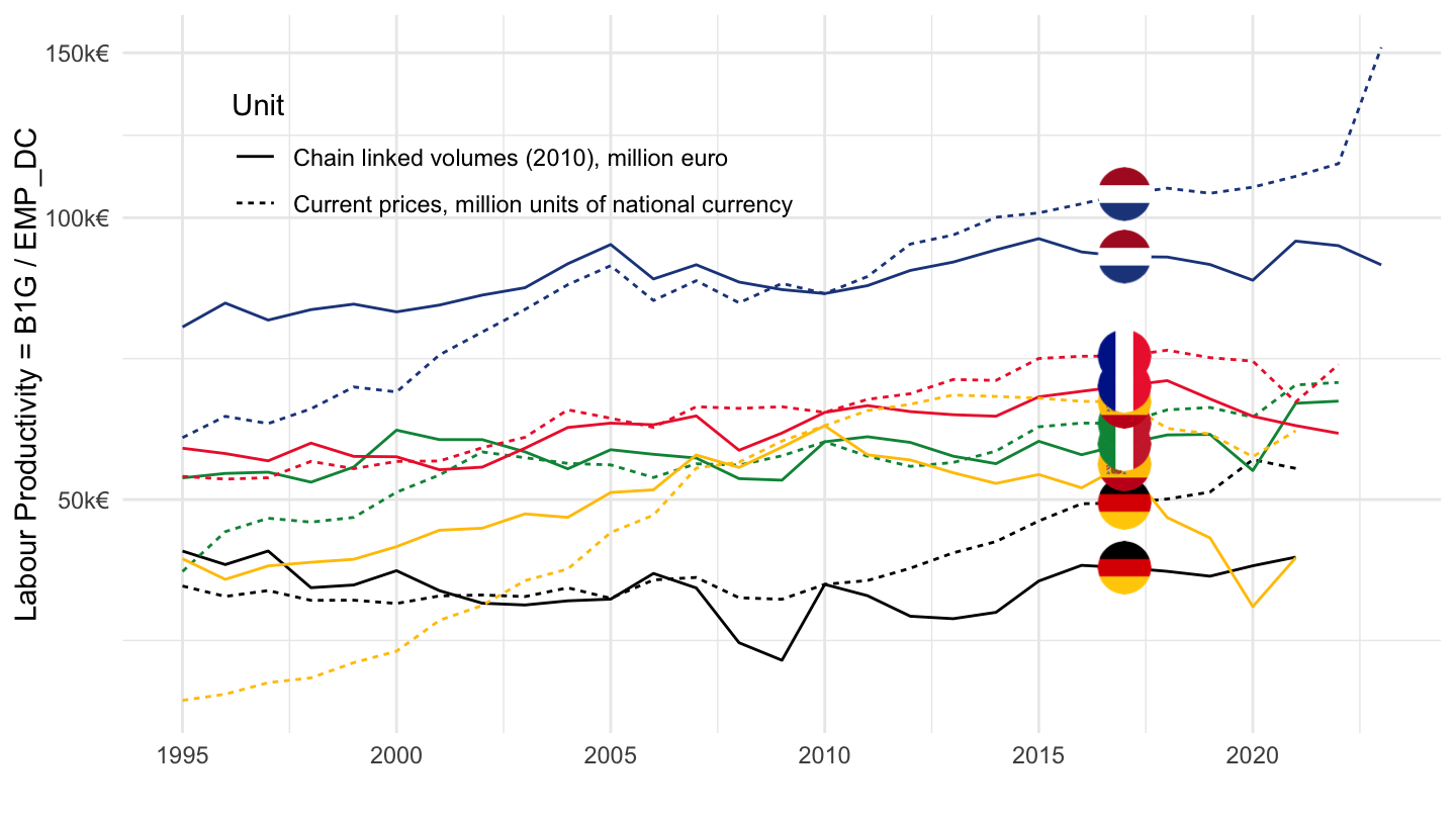
Base 100
Code
nama_10_a64 %>%
  filter(na_item == "B1G",
         nace_r2 %in% c("C10-C12"),
         geo %in% c("FR", "DE", "IT", "ES", "NL"),
         unit %in% c("CP_MNAC", "CLV10_MEUR")) %>%
  select_if(~ n_distinct(.) > 1) %>%
  rename(B1G = values) %>%
  left_join(nama_10_a64_e %>%
              filter(nace_r2 %in% c("C10-C12"),
                     geo %in% c("FR", "DE", "IT", "ES", "NL"),
                     unit == "THS_PER",
                     na_item == "EMP_DC") %>%
              select_if(~ n_distinct(.) > 1) %>%
              rename(EMP_DC = values), by = c("geo", "Geo", "time")) %>%
  mutate(values = B1G/EMP_DC) %>%
  year_to_date() %>%
  filter(date >= as.Date("1995-01-01")) %>%


  left_join(colors, by = c("Geo" = "country")) %>%
  mutate(color = ifelse(geo == "NL", color2, color)) %>%
  group_by(Geo, Unit) %>%
  arrange(date) %>%
  mutate(values = 100*values/values[1]) %>%
  ggplot(.) + geom_line(aes(x = date, y = values, color = color, linetype = Unit)) +
  theme_minimal() + xlab("") + ylab("Labour Productivity = B1G / EMP_DC") +
  scale_color_identity() + add_flags +
  scale_x_date(breaks = seq(1960, 2100, 5) %>% paste0("-01-01") %>% as.Date,
               labels = date_format("%Y")) +
  theme(legend.position = c(0.3, 0.8)) +
  scale_y_log10(breaks = seq(0, 2000, 20))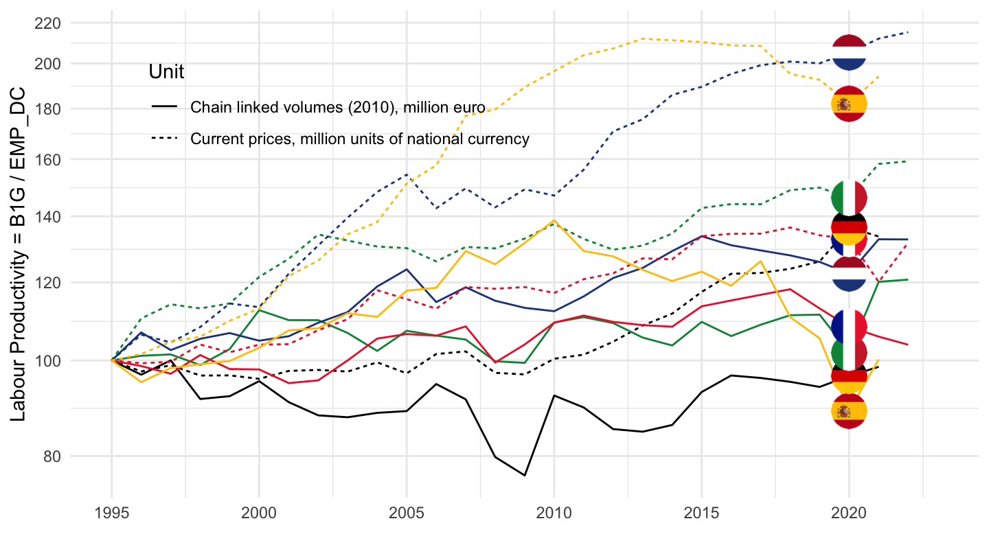
C13-C15 - Textiles
Value
All
Code
nama_10_a64_e %>%
  filter(nace_r2 %in% c("C13-C15", "TOTAL"),
         geo %in% c("FR", "DE", "IT", "ES"),
         unit == "THS_PER",
         na_item == "EMP_DC") %>%
  year_to_date() %>%

  select(geo,  Geo, nace_r2, date, values) %>%
  spread(nace_r2, values) %>%
  mutate(values = `C13-C15`/TOTAL) %>%
  left_join(colors, by = c("Geo" = "country")) %>%
  ggplot(.) + geom_line(aes(x = date, y = values, color = color)) +
  theme_minimal() + xlab("") + ylab("Textiles (% of GDP)") +
  scale_color_identity() + add_4flags +
  scale_x_date(breaks = seq(1960, 2100, 5) %>% paste0("-01-01") %>% as.Date,
               labels = date_format("%Y")) +
  theme(legend.position = "none") +
  scale_y_continuous(breaks = 0.01*seq(-500, 200, 0.1),
                     labels = percent_format(accuracy = .1))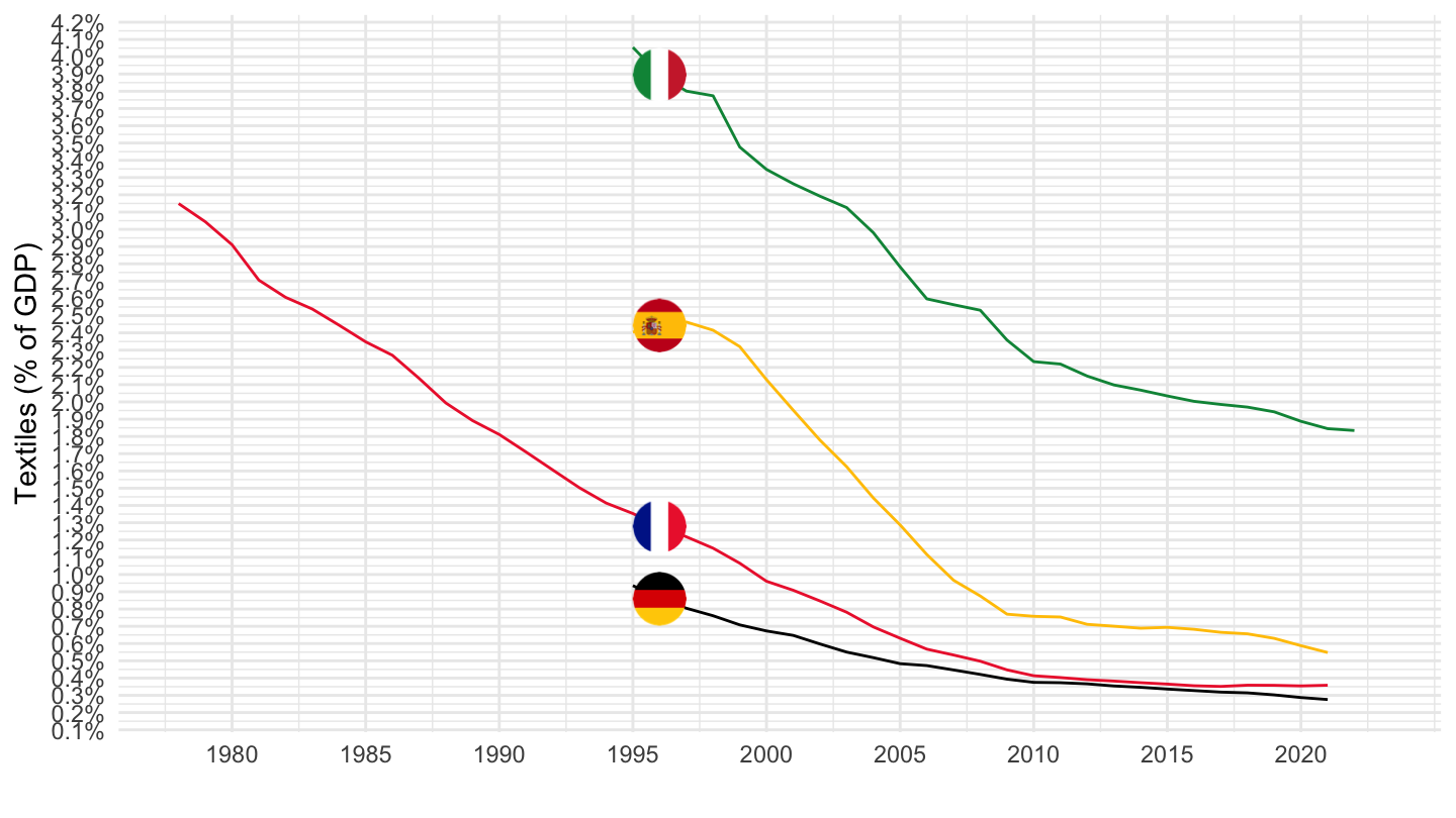
1995-
Code
nama_10_a64_e %>%
  filter(nace_r2 %in% c("C13-C15", "TOTAL"),
         geo %in% c("FR", "DE", "IT", "ES"),
         unit == "THS_PER",
         na_item == "EMP_DC") %>%
  year_to_date() %>%
  filter(date >= as.Date("1995-01-01")) %>%

  select(geo,  Geo, nace_r2, date, values) %>%
  spread(nace_r2, values) %>%
  mutate(values = `C13-C15`/TOTAL) %>%
  left_join(colors, by = c("Geo" = "country")) %>%
  ggplot(.) + geom_line(aes(x = date, y = values, color = color)) +
  theme_minimal() + xlab("") + ylab("Textiles (% of GDP)") +
  scale_color_identity() + add_4flags +
  scale_x_date(breaks = seq(1960, 2100, 5) %>% paste0("-01-01") %>% as.Date,
               labels = date_format("%Y")) +
  theme(legend.position = "none") +
  scale_y_continuous(breaks = 0.01*seq(-500, 200, 0.1),
                     labels = percent_format(accuracy = .1))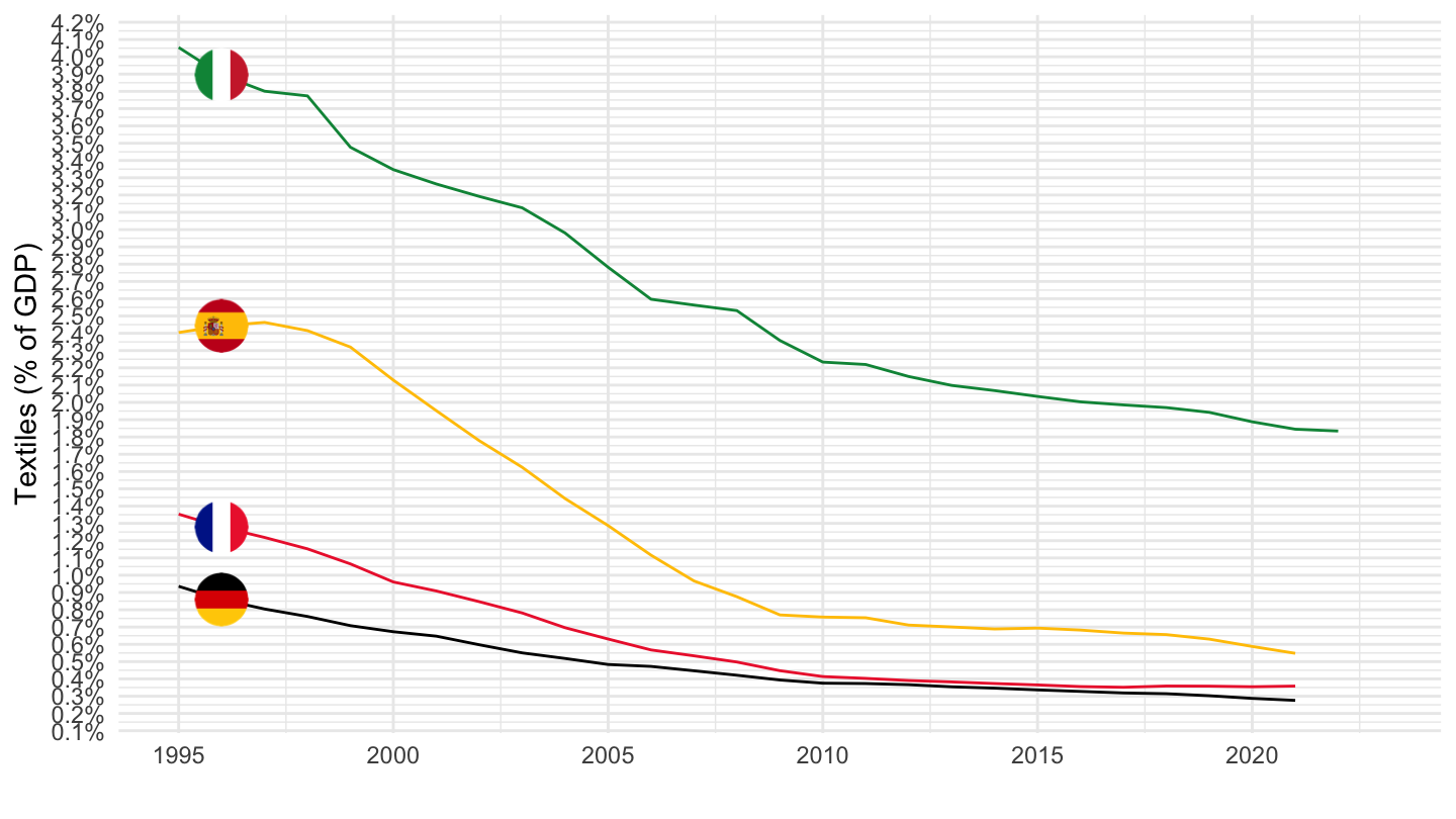
C21 - Manufacture of basic pharmaceutical products and pharmaceutical preparations
Value
All
Code
nama_10_a64_e %>%
  filter(nace_r2 %in% c("C21", "TOTAL"),
         geo %in% c("FR", "DE", "IT", "ES"),
         unit == "THS_PER",
         na_item == "EMP_DC") %>%
  year_to_date() %>%

  select(geo,  Geo, nace_r2, date, values) %>%
  spread(nace_r2, values) %>%
  mutate(values = `C21`/TOTAL) %>%
  left_join(colors, by = c("Geo" = "country")) %>%
  ggplot(.) + geom_line(aes(x = date, y = values, color = color)) +
  theme_minimal() + xlab("") + ylab("Manufacture of basic pharmaceutical products (% of GDP)") +
  scale_color_identity() + add_4flags +
  scale_x_date(breaks = seq(1960, 2100, 5) %>% paste0("-01-01") %>% as.Date,
               labels = date_format("%Y")) +
  theme(legend.position = "none") +
  scale_y_continuous(breaks = 0.01*seq(-500, 200, 0.02),
                     labels = percent_format(accuracy = .01))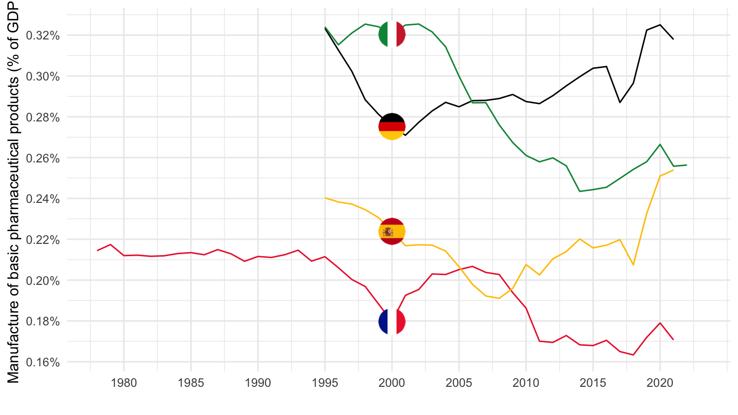
1995-
% of employment
Code
nama_10_a64_e %>%
  filter(nace_r2 %in% c("C21", "TOTAL"),
         geo %in% c("FR", "DE", "IT", "ES", "NL"),
         unit == "THS_PER",
         na_item == "EMP_DC") %>%
  year_to_date() %>%
  filter(date >= as.Date("1995-01-01")) %>%

  select(geo,  Geo, nace_r2, date, values) %>%
  spread(nace_r2, values) %>%
  mutate(values = `C21`/TOTAL) %>%
  left_join(colors, by = c("Geo" = "country")) %>%
  ggplot(.) + geom_line(aes(x = date, y = values, color = color)) +
  theme_minimal() + xlab("") + ylab("Manufacture of basic pharmaceutical products\n % of Employment") +
  scale_color_identity() + add_5flags +
  scale_x_date(breaks = seq(1960, 2100, 5) %>% paste0("-01-01") %>% as.Date,
               labels = date_format("%Y")) +
  theme(legend.position = "none") +
  scale_y_continuous(breaks = 0.01*seq(-500, 200, 0.02),
                     labels = percent_format(accuracy = .01))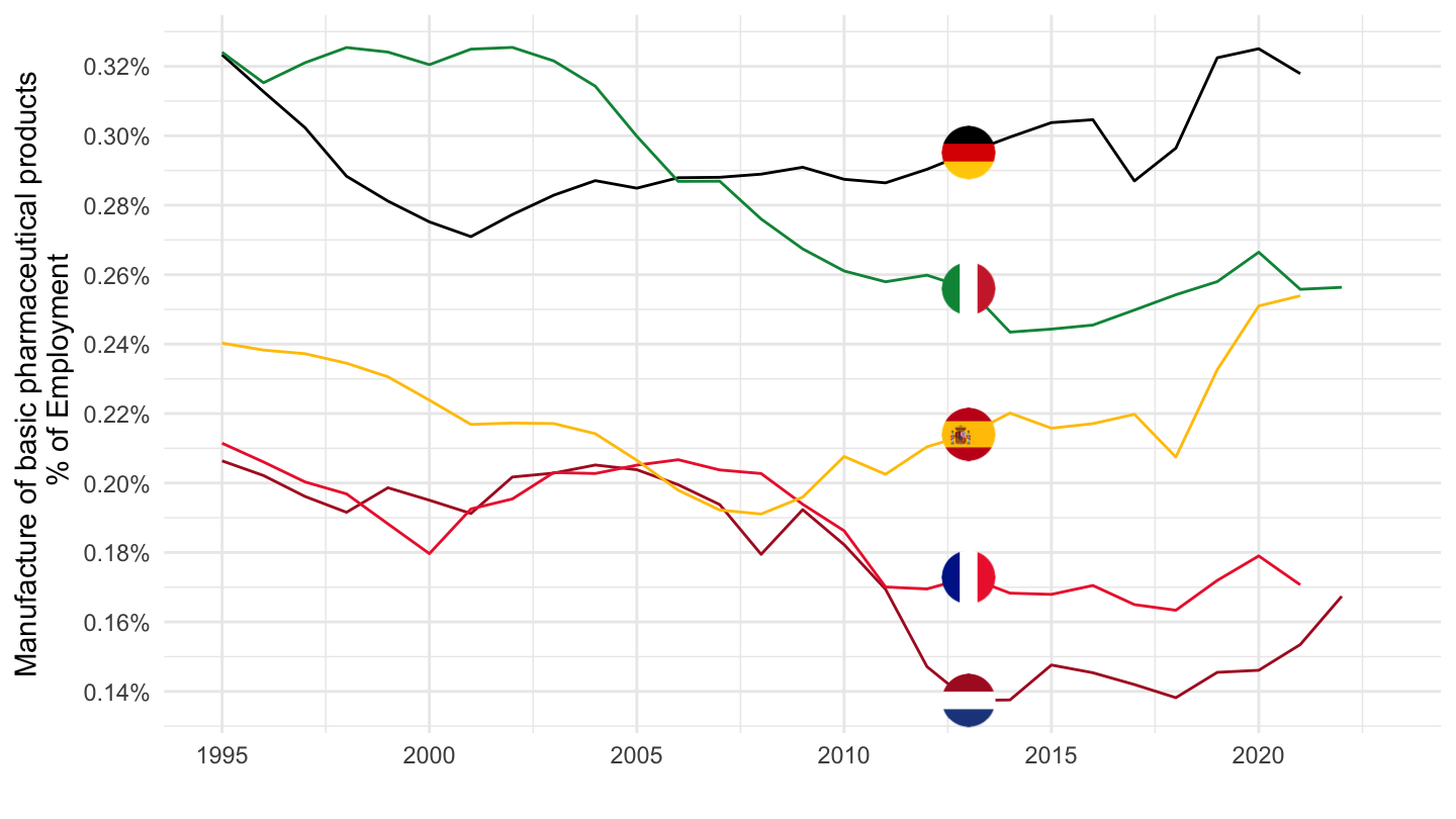
Productivity
Normal
Code
nama_10_a64 %>%
  filter(na_item == "B1G",
         nace_r2 %in% c("C21"),
         geo %in% c("FR", "DE", "IT", "ES", "NL"),
         unit %in% c("CP_MNAC", "CLV10_MEUR")) %>%
  select_if(~ n_distinct(.) > 1) %>%
  rename(B1G = values) %>%
  left_join(nama_10_a64_e %>%
              filter(nace_r2 %in% c("C21"),
                     geo %in% c("FR", "DE", "IT", "ES", "NL"),
                     unit == "THS_PER",
                     na_item == "EMP_DC") %>%
              select_if(~ n_distinct(.) > 1) %>%
              rename(EMP_DC = values), by = c("geo", "Geo", "time")) %>%
  mutate(values = B1G/EMP_DC) %>%
  year_to_date() %>%
  filter(date >= as.Date("1995-01-01")) %>%


  left_join(colors, by = c("Geo" = "country")) %>%
  mutate(color = ifelse(geo == "NL", color2, color)) %>%
  ggplot(.) + geom_line(aes(x = date, y = values, color = color, linetype = Unit)) +
  theme_minimal() + xlab("") + ylab("Manufacture of basic pharmaceutical products\n Labour Productivity = B1G / EMP_DC") +
  scale_color_identity() + add_flags +
  scale_x_date(breaks = seq(1960, 2100, 5) %>% paste0("-01-01") %>% as.Date,
               labels = date_format("%Y")) +
  theme(legend.position = c(0.3, 0.8)) +
  scale_y_continuous(breaks = seq(0, 2000, 50),
                     labels = dollar_format(pre = "", su = "k€", acc = 1))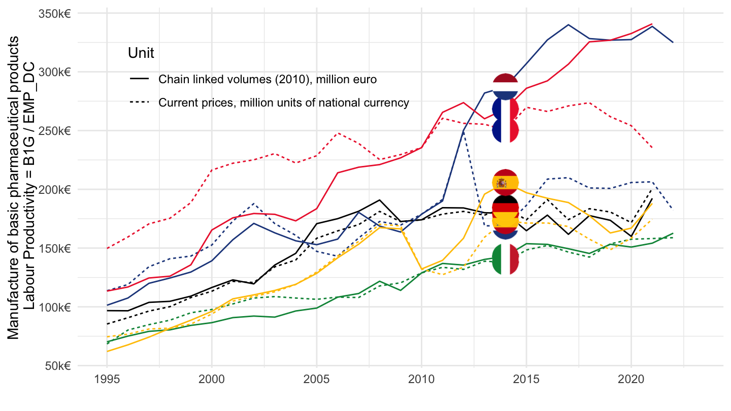
Log
Code
nama_10_a64 %>%
  filter(na_item == "B1G",
         nace_r2 %in% c("C21"),
         geo %in% c("FR", "DE", "IT", "ES", "NL"),
         unit %in% c("CP_MNAC", "CLV10_MEUR")) %>%
  select_if(~ n_distinct(.) > 1) %>%
  rename(B1G = values) %>%
  left_join(nama_10_a64_e %>%
              filter(nace_r2 %in% c("C21"),
                     geo %in% c("FR", "DE", "IT", "ES", "NL"),
                     unit == "THS_PER",
                     na_item == "EMP_DC") %>%
              select_if(~ n_distinct(.) > 1) %>%
              rename(EMP_DC = values), by = c("geo", "Geo", "time")) %>%
  mutate(values = B1G/EMP_DC) %>%
  year_to_date() %>%
  filter(date >= as.Date("1995-01-01")) %>%


  left_join(colors, by = c("Geo" = "country")) %>%
  mutate(color = ifelse(geo == "NL", color2, color)) %>%
  ggplot(.) + geom_line(aes(x = date, y = values, color = color, linetype = Unit)) +
  theme_minimal() + xlab("") + ylab("Manufacture of basic pharmaceutical products\n Labour Productivity = B1G / EMP_DC") +
  scale_color_identity() + add_flags +
  scale_x_date(breaks = seq(1960, 2100, 5) %>% paste0("-01-01") %>% as.Date,
               labels = date_format("%Y")) +
  theme(legend.position = c(0.3, 0.8)) +
  scale_y_log10(breaks = seq(0, 2000, 50),
                     labels = dollar_format(pre = "", su = "k€", acc = 1))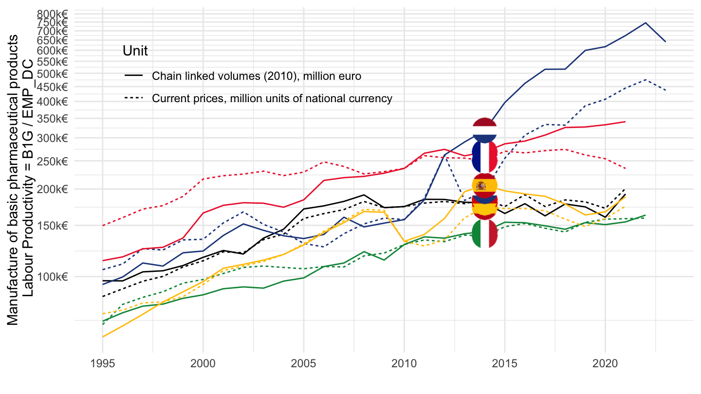
Base 100
Code
nama_10_a64 %>%
  filter(na_item == "B1G",
         nace_r2 %in% c("C21"),
         geo %in% c("FR", "DE", "IT", "ES", "NL"),
         unit %in% c("CP_MNAC", "CLV10_MEUR")) %>%
  select_if(~ n_distinct(.) > 1) %>%
  rename(B1G = values) %>%
  left_join(nama_10_a64_e %>%
              filter(nace_r2 %in% c("C21"),
                     geo %in% c("FR", "DE", "IT", "ES", "NL"),
                     unit == "THS_PER",
                     na_item == "EMP_DC") %>%
              select_if(~ n_distinct(.) > 1) %>%
              rename(EMP_DC = values), by = c("geo", "Geo", "time")) %>%
  mutate(values = B1G/EMP_DC) %>%
  year_to_date() %>%
  filter(date >= as.Date("1995-01-01")) %>%


  left_join(colors, by = c("Geo" = "country")) %>%
  mutate(color = ifelse(geo == "NL", color2, color)) %>%
  group_by(Geo, Unit) %>%
  arrange(date) %>%
  mutate(values = 100*values/values[1]) %>%
  ggplot(.) + geom_line(aes(x = date, y = values, color = color, linetype = Unit)) +
  theme_minimal() + xlab("") + ylab("Manufacture of basic pharmaceutical products\n Labour Productivity = B1G / EMP_DC") +
  scale_color_identity() + add_flags +
  scale_x_date(breaks = seq(1960, 2100, 5) %>% paste0("-01-01") %>% as.Date,
               labels = date_format("%Y")) +
  theme(legend.position = c(0.3, 0.8)) +
  scale_y_log10(breaks = seq(0, 2000, 20))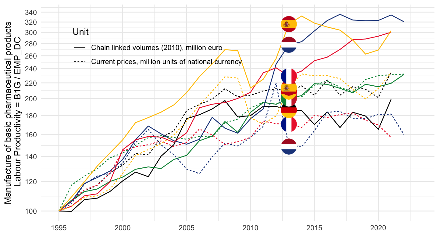
C16-C18 - Wood, Paper, Printing
All
Code
nama_10_a64_e %>%
  filter(nace_r2 %in% c("C16-C18", "TOTAL"),
         geo %in% c("FR", "DE", "IT", "ES"),
         unit == "THS_PER",
         na_item == "EMP_DC") %>%
  year_to_date() %>%

  select(geo,  Geo, nace_r2, date, values) %>%
  spread(nace_r2, values) %>%
  ggplot(.) + geom_line(aes(x = date, y = `C16-C18`/TOTAL, color = Geo)) +
  theme_minimal() + xlab("") + ylab("Wood, Paper, Printing (% of GDP)") +
  scale_color_manual(values = c("#002395", "#000000", "#009246", "#C60B1E")) +
  scale_x_date(breaks = seq(1960, 2100, 5) %>% paste0("-01-01") %>% as.Date,
               labels = date_format("%Y")) +
  geom_image(data = . %>%
               filter(date == as.Date("2017-01-01")) %>%
               mutate(image = paste0("../../icon/flag/round/", str_to_lower(Geo), ".png")),
             aes(x = date, y = `C16-C18`/TOTAL, image = image), asp = 1.5) +
  theme(legend.position = "none") +
  scale_y_continuous(breaks = 0.01*seq(-500, 200, 0.1),
                     labels = percent_format(accuracy = .1))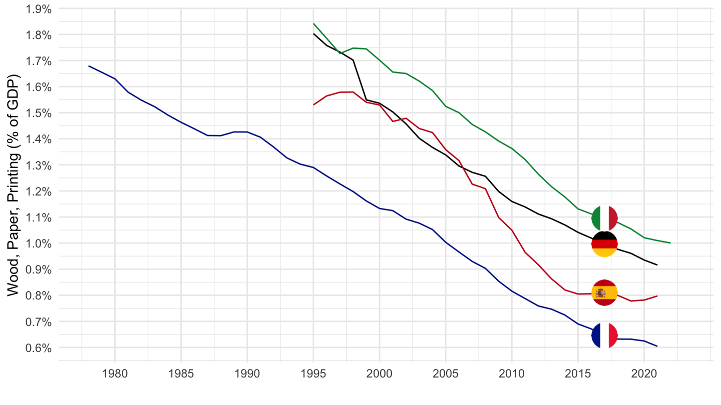
1995-
Code
nama_10_a64_e %>%
  filter(nace_r2 %in% c("C16-C18", "TOTAL"),
         geo %in% c("FR", "DE", "IT", "ES"),
         unit == "THS_PER",
         na_item == "EMP_DC") %>%
  year_to_date() %>%
  filter(date >= as.Date("1995-01-01")) %>%

  select(geo,  Geo, nace_r2, date, values) %>%
  spread(nace_r2, values) %>%
  ggplot(.) + geom_line(aes(x = date, y = `C16-C18`/TOTAL, color = Geo)) +
  theme_minimal() + xlab("") + ylab("Wood, Paper, Printing (% of GDP)") +
  scale_color_manual(values = c("#002395", "#000000", "#009246", "#C60B1E")) +
  scale_x_date(breaks = seq(1960, 2100, 2) %>% paste0("-01-01") %>% as.Date,
               labels = date_format("%Y")) +
  geom_image(data = . %>%
               filter(date == as.Date("2017-01-01")) %>%
               mutate(image = paste0("../../icon/flag/round/", str_to_lower(Geo), ".png")),
             aes(x = date, y = `C16-C18`/TOTAL, image = image), asp = 1.5) +
  theme(legend.position = "none") +
  scale_y_continuous(breaks = 0.01*seq(-500, 200, 0.1),
                     labels = percent_format(accuracy = .1))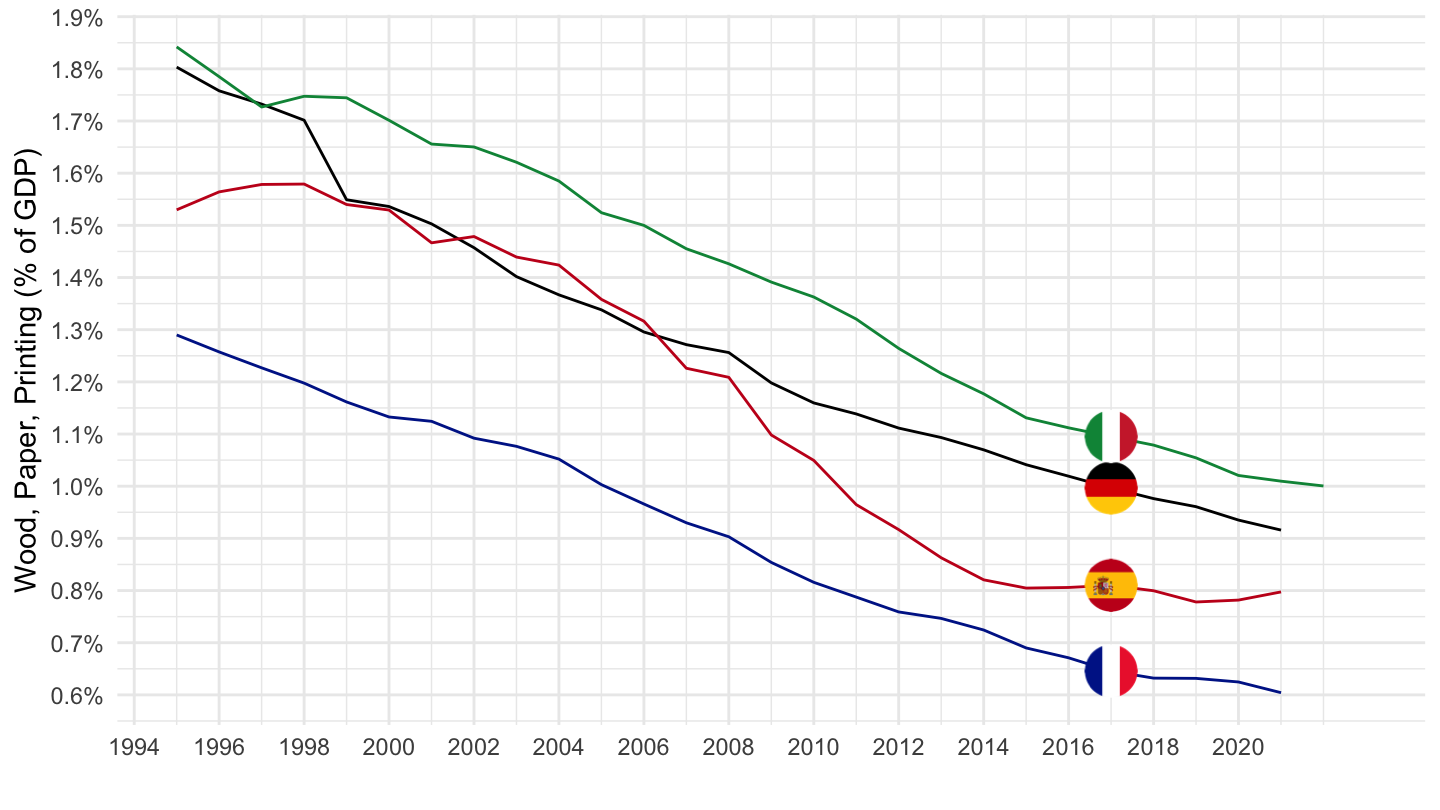
C29 - Motor vehicles
France, Europe
All
Code
# load_data("eurostat/nace_r2_fr.RData")
nama_10_a64_e %>%
  filter(nace_r2 %in% c("C29", "TOTAL"),
         geo %in% c("FR", "EA20"),
         unit == "THS_PER",
         na_item == "EMP_DC") %>%
  year_to_date() %>%
  #filter(date >= as.Date("1995-01-01")) %>%

  mutate(Geo = ifelse(geo == "EA20", "Europe", Geo)) %>%
  select(geo,  Geo, nace_r2, date, values) %>%
  spread(nace_r2, values) %>%
  mutate(values = `C29`/TOTAL) %>%
  filter(!is.na(values)) %>%
  left_join(colors, by = c("Geo" = "country")) %>%
  ggplot(.) + geom_line(aes(x = date, y = values, color = color)) +
  theme_minimal() + xlab("") + ylab("Industrie automobile (% de l'emploi)") +
  scale_color_identity() +
  scale_x_date(breaks = seq(1960, 2100, 5) %>% paste0("-01-01") %>% as.Date,
               labels = date_format("%Y")) + add_2flags +
  theme(legend.position = "none") +
  scale_y_continuous(breaks = 0.01*seq(-500, 200, 0.1),
                     labels = percent_format(accuracy = .1))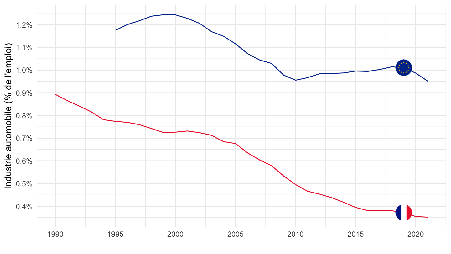
1995-
Code
# load_data("eurostat/nace_r2_fr.RData")
nama_10_a64_e %>%
  filter(nace_r2 %in% c("C29", "TOTAL"),
         geo %in% c("FR", "EA20"),
         unit == "THS_PER",
         na_item == "EMP_DC") %>%
  year_to_date() %>%
  filter(date >= as.Date("1995-01-01")) %>%

  mutate(Geo = ifelse(geo == "EA20", "Europe", Geo)) %>%
  select(geo,  Geo, nace_r2, date, values) %>%
  spread(nace_r2, values) %>%
  mutate(values = `C29`/TOTAL) %>%
  filter(!is.na(values)) %>%
  left_join(colors, by = c("Geo" = "country")) %>%
  ggplot(.) + geom_line(aes(x = date, y = values, color = color)) +
  theme_minimal() + xlab("") + ylab("Industrie automobile (% de l'emploi)") +
  scale_color_identity() +
  scale_x_date(breaks = seq(1960, 2100, 5) %>% paste0("-01-01") %>% as.Date,
               labels = date_format("%Y")) + add_2flags +
  theme(legend.position = "none") +
  scale_y_continuous(breaks = 0.01*seq(-500, 200, 0.1),
                     labels = percent_format(accuracy = .1))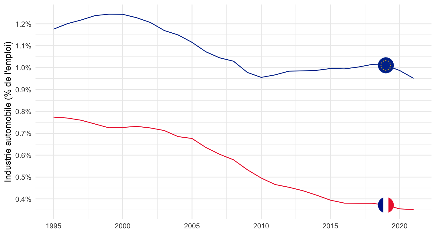
All
Code
nama_10_a64_e %>%
  filter(nace_r2 %in% c("C29", "TOTAL"),
         geo %in% c("FR", "DE", "IT", "ES"),
         unit == "THS_PER",
         na_item == "EMP_DC") %>%
  year_to_date() %>%

  select(geo,  Geo, nace_r2, date, values) %>%
  spread(nace_r2, values) %>%
  ggplot(.) + geom_line(aes(x = date, y = `C29`/TOTAL, color = Geo)) +
  theme_minimal() + xlab("") + ylab("Motor vehicles (% of GDP)") +
  scale_color_manual(values = c("#002395", "#000000", "#009246", "#C60B1E")) +
  scale_x_date(breaks = seq(1960, 2100, 5) %>% paste0("-01-01") %>% as.Date,
               labels = date_format("%Y")) +
  geom_image(data = . %>%
               filter(date == as.Date("2017-01-01")) %>%
               mutate(image = paste0("../../icon/flag/round/", str_to_lower(Geo), ".png")),
             aes(x = date, y = `C29`/TOTAL, image = image), asp = 1.5) +
  theme(legend.position = "none") +
  scale_y_continuous(breaks = 0.01*seq(-500, 200, 0.5),
                     labels = percent_format(accuracy = .1))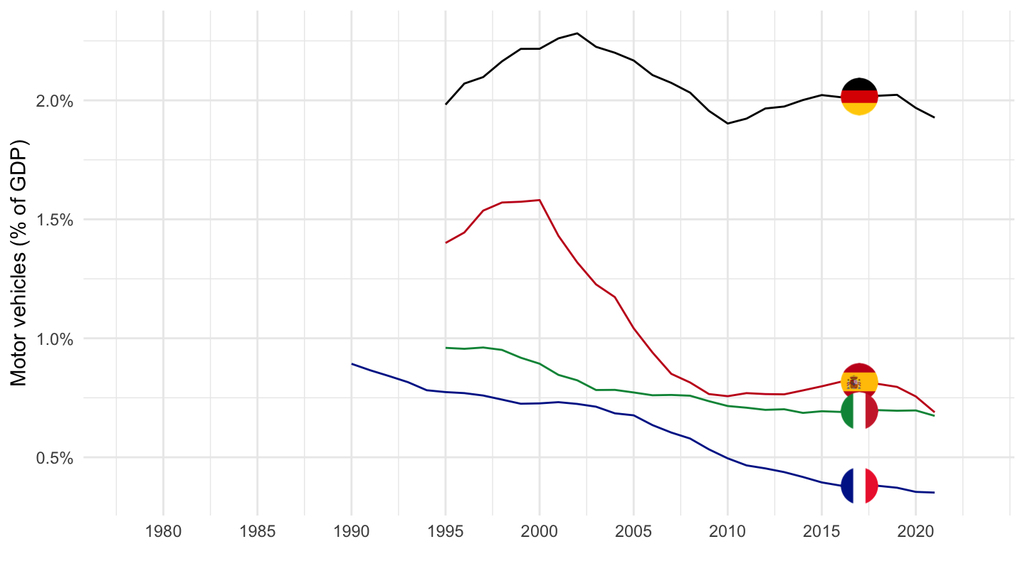
1995-
Code
nama_10_a64_e %>%
  filter(nace_r2 %in% c("C29", "TOTAL"),
         geo %in% c("FR", "DE", "IT", "ES"),
         unit == "THS_PER",
         na_item == "EMP_DC") %>%
  year_to_date() %>%
  filter(date >= as.Date("1995-01-01")) %>%

  select(geo,  Geo, nace_r2, date, values) %>%
  spread(nace_r2, values) %>%
  ggplot(.) + geom_line(aes(x = date, y = `C29`/TOTAL, color = Geo)) +
  theme_minimal() + xlab("") + ylab("Motor vehicles (% of GDP)") +
  scale_color_manual(values = c("#002395", "#000000", "#009246", "#C60B1E")) +
  scale_x_date(breaks = seq(1960, 2100, 2) %>% paste0("-01-01") %>% as.Date,
               labels = date_format("%Y")) +
  geom_image(data = . %>%
               filter(date == as.Date("2017-01-01")) %>%
               mutate(image = paste0("../../icon/flag/round/", str_to_lower(Geo), ".png")),
             aes(x = date, y = `C29`/TOTAL, image = image), asp = 1.5) +
  theme(legend.position = "none") +
  scale_y_continuous(breaks = 0.01*seq(-500, 200, 0.5),
                     labels = percent_format(accuracy = .1))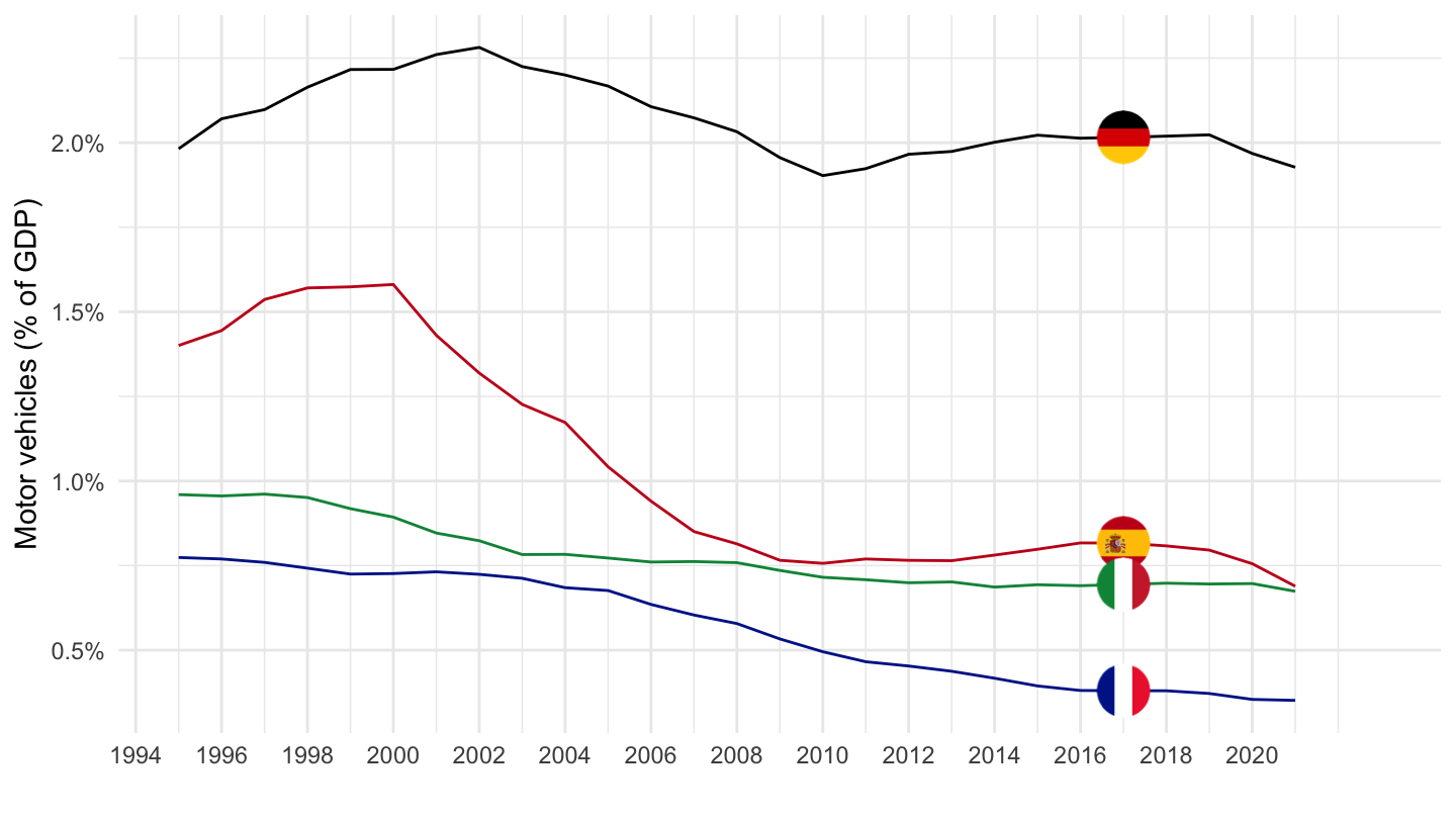
C29_C30 - Motor vehicles and other transport equipment
All
Code
nama_10_a64_e %>%
  filter(nace_r2 %in% c("C29_C30", "TOTAL"),
         geo %in% c("FR", "DE", "IT", "ES"),
         unit == "THS_PER",
         na_item == "EMP_DC") %>%
  year_to_date() %>%

  select(geo,  Geo, nace_r2, date, values) %>%
  spread(nace_r2, values) %>%
  mutate(values = `C29_C30`/TOTAL) %>%
  ggplot(.) + geom_line(aes(x = date, y = values, color = Geo)) +
  theme_minimal() + xlab("") + ylab("Motor vehicles and other transport equipment") +
  scale_color_manual(values = c("#002395", "#000000", "#009246", "#C60B1E")) +
  scale_x_date(breaks = seq(1960, 2100, 5) %>% paste0("-01-01") %>% as.Date,
               labels = date_format("%Y")) + add_4flags +
  theme(legend.position = "none") +
  scale_y_continuous(breaks = 0.01*seq(-500, 200, 0.5),
                     labels = percent_format(accuracy = .1))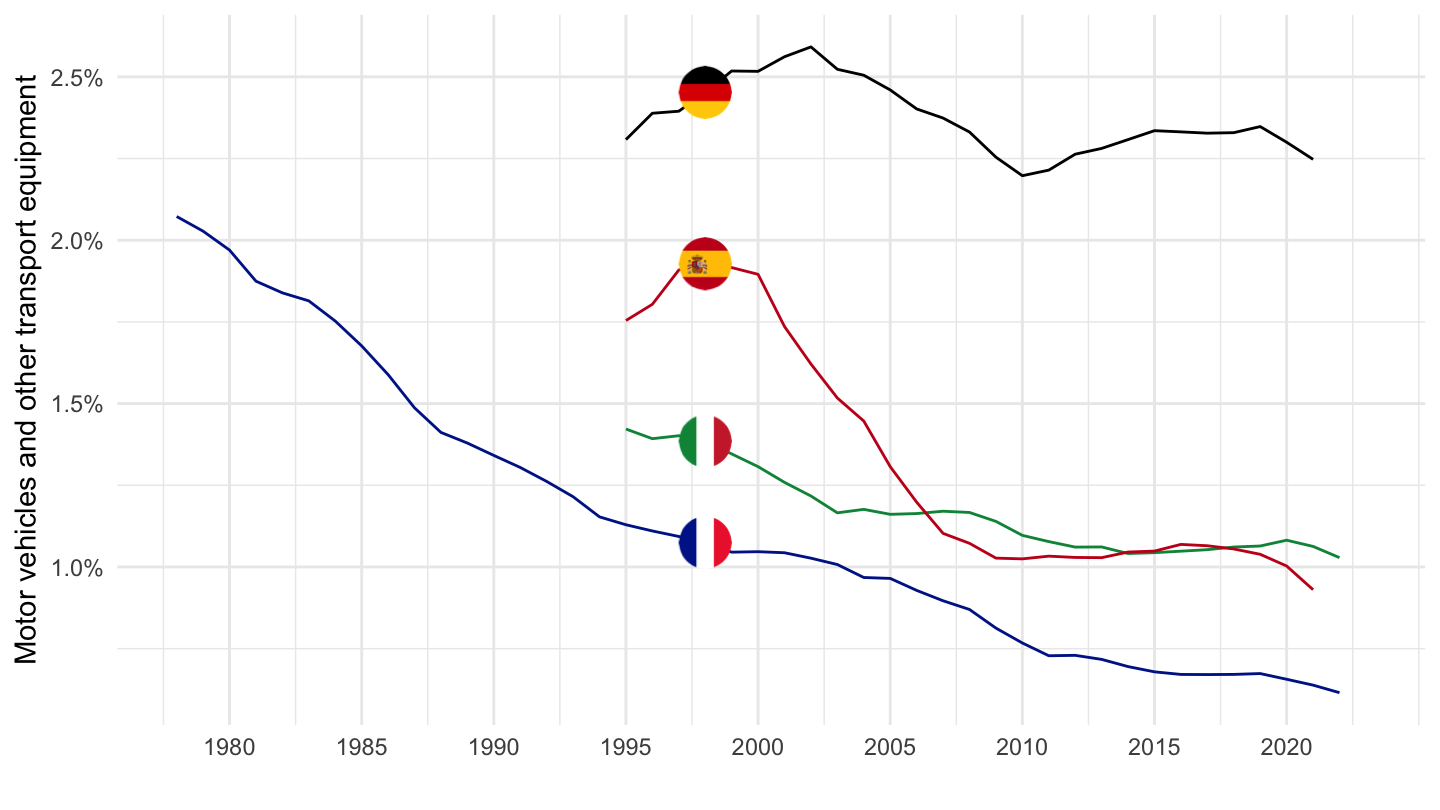
1995-
Code
nama_10_a64_e %>%
  filter(nace_r2 %in% c("C29_C30", "TOTAL"),
         geo %in% c("FR", "DE", "IT", "ES"),
         unit == "THS_PER",
         na_item == "EMP_DC") %>%
  year_to_date() %>%
  filter(date >= as.Date("1995-01-01")) %>%

  select(geo,  Geo, nace_r2, date, values) %>%
  spread(nace_r2, values) %>%
  ggplot(.) + geom_line(aes(x = date, y = `C29_C30`/TOTAL, color = Geo)) +
  theme_minimal() + xlab("") + ylab("Motor vehicles and other transport equipment (% of GDP)") +
  scale_color_manual(values = c("#002395", "#000000", "#009246", "#C60B1E")) +
  scale_x_date(breaks = seq(1960, 2100, 2) %>% paste0("-01-01") %>% as.Date,
               labels = date_format("%Y")) +
  geom_image(data = . %>%
               filter(date == as.Date("2017-01-01")) %>%
               mutate(image = paste0("../../icon/flag/round/", str_to_lower(Geo), ".png")),
             aes(x = date, y = `C29_C30`/TOTAL, image = image), asp = 1.5) +
  theme(legend.position = "none") +
  scale_y_continuous(breaks = 0.01*seq(-500, 200, 0.5),
                     labels = percent_format(accuracy = .1))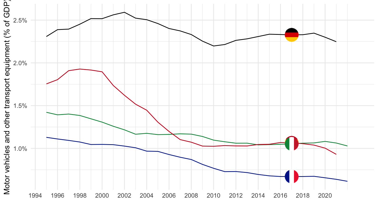
C28 - Machinery and equipment
All
Code
nama_10_a64_e %>%
  filter(nace_r2 %in% c("C28", "TOTAL"),
         geo %in% c("FR", "DE", "IT", "ES"),
         unit == "THS_PER",
         na_item == "EMP_DC") %>%
  year_to_date() %>%

  select(geo,  Geo, nace_r2, date, values) %>%
  spread(nace_r2, values) %>%
  mutate(values = `C28`/TOTAL) %>%
  ggplot(.) + geom_line(aes(x = date, y = values, color = Geo)) +
  theme_minimal() + xlab("") + ylab("Machinery and equipment (% of GDP)") +
  scale_color_manual(values = c("#002395", "#000000", "#009246", "#C60B1E")) +
  scale_x_date(breaks = seq(1960, 2100, 5) %>% paste0("-01-01") %>% as.Date,
               labels = date_format("%Y")) + add_4flags +
  theme(legend.position = "none") +
  scale_y_continuous(breaks = 0.01*seq(-500, 200, 0.1),
                     labels = percent_format(accuracy = .1))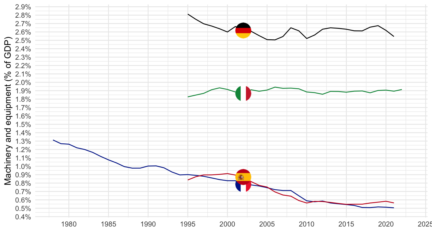
1995-
Code
nama_10_a64_e %>%
  filter(nace_r2 %in% c("C28", "TOTAL"),
         geo %in% c("FR", "DE", "IT", "ES"),
         unit == "THS_PER",
         na_item == "EMP_DC") %>%
  year_to_date() %>%
  filter(date >= as.Date("1995-01-01")) %>%

  select(geo,  Geo, nace_r2, date, values) %>%
  spread(nace_r2, values) %>%
  mutate(values = `C28`/TOTAL) %>%
  ggplot(.) + geom_line(aes(x = date, y = values, color = Geo)) +
  theme_minimal() + xlab("") + ylab("Machinery and equipment (% of GDP)") +
  scale_color_manual(values = c("#002395", "#000000", "#009246", "#C60B1E")) +
  scale_x_date(breaks = seq(1960, 2100, 2) %>% paste0("-01-01") %>% as.Date,
               labels = date_format("%Y")) + add_4flags +
  theme(legend.position = "none") +
  scale_y_continuous(breaks = 0.01*seq(-500, 200, 0.1),
                     labels = percent_format(accuracy = .1))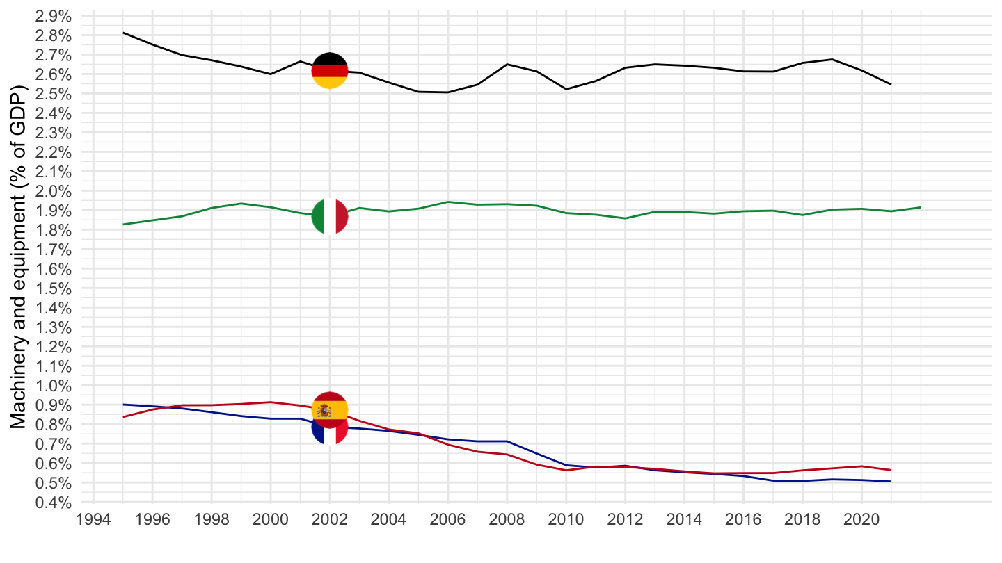
L - Real Estate
Value
Code
nama_10_a64_e %>%
  filter(nace_r2 %in% c("L", "TOTAL"),
         geo %in% c("FR", "DE", "IT", "ES"),
         unit == "THS_PER",
         na_item == "EMP_DC") %>%
  year_to_date() %>%

  select(geo,  Geo, nace_r2, date, values) %>%
  spread(nace_r2, values) %>%
  mutate(values = `L`/TOTAL) %>%
  left_join(colors, by = c("Geo" = "country")) %>%
  ggplot(.) + geom_line(aes(x = date, y = values, color = color)) +
  theme_minimal() + xlab("") + ylab("Real Estate (% of GDP)") +
  scale_color_identity() + add_4flags +
  scale_x_date(breaks = seq(1960, 2100, 5) %>% paste0("-01-01") %>% as.Date,
               labels = date_format("%Y")) +
  scale_y_continuous(breaks = 0.01*seq(-500, 200, .1),
                     labels = percent_format(accuracy = .1))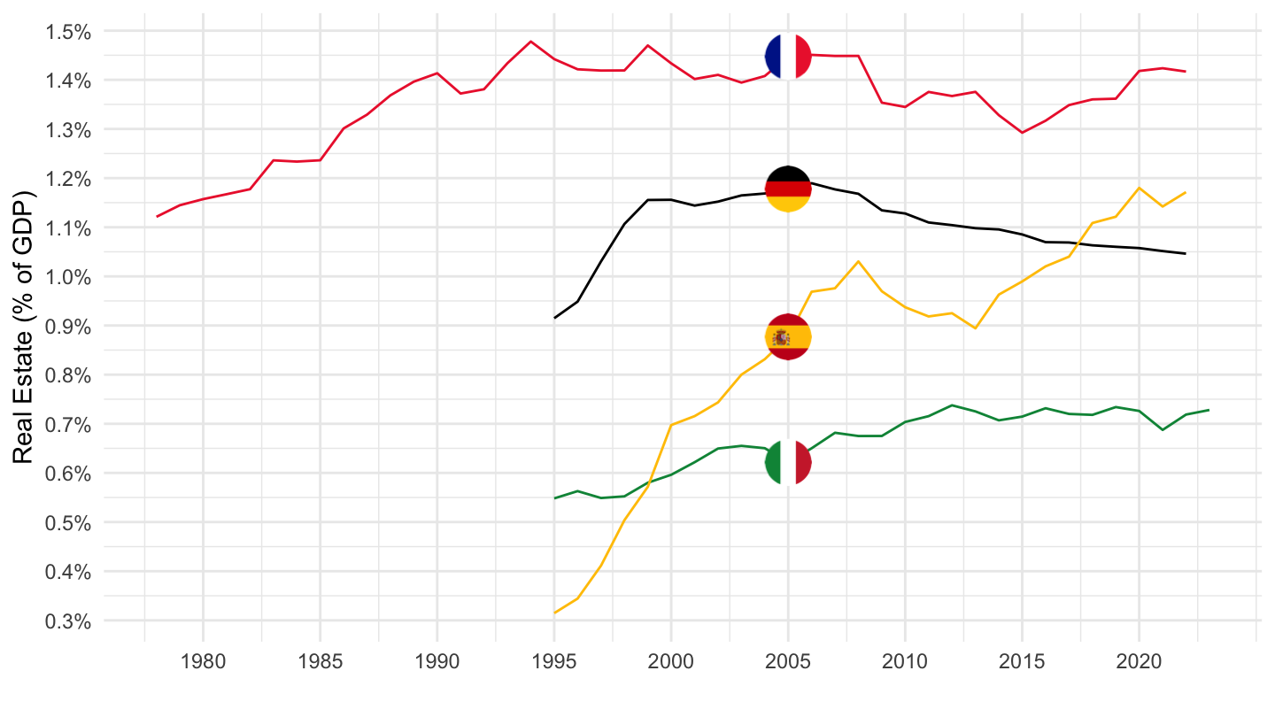
Productivity
Normal
Code
nama_10_a64 %>%
  filter(na_item == "B1G",
         nace_r2 %in% c("L"),
         geo %in% c("FR", "DE", "IT", "ES", "NL"),
         unit %in% c("CP_MNAC", "CLV10_MEUR")) %>%
  select_if(~ n_distinct(.) > 1) %>%
  rename(B1G = values) %>%
  left_join(nama_10_a64_e %>%
              filter(nace_r2 %in% c("L"),
                     geo %in% c("FR", "DE", "IT", "ES", "NL"),
                     unit == "THS_PER",
                     na_item == "EMP_DC") %>%
              select_if(~ n_distinct(.) > 1) %>%
              rename(EMP_DC = values), by = c("geo", "Geo", "time")) %>%
  mutate(values = B1G/EMP_DC) %>%
  year_to_date() %>%
  filter(date >= as.Date("1995-01-01")) %>%


  left_join(colors, by = c("Geo" = "country")) %>%
  mutate(color = ifelse(geo == "NL", color2, color)) %>%
  ggplot(.) + geom_line(aes(x = date, y = values, color = color, linetype = Unit)) +
  theme_minimal() + xlab("") + ylab("Labour Productivity = B1G / EMP_DC") +
  scale_color_identity() + add_flags +
  scale_x_date(breaks = seq(1960, 2100, 5) %>% paste0("-01-01") %>% as.Date,
               labels = date_format("%Y")) +
  theme(legend.position = c(0.3, 0.8)) +
  scale_y_continuous(breaks = seq(0, 2000, 50),
                     labels = dollar_format(pre = "", su = "k€", acc = 1))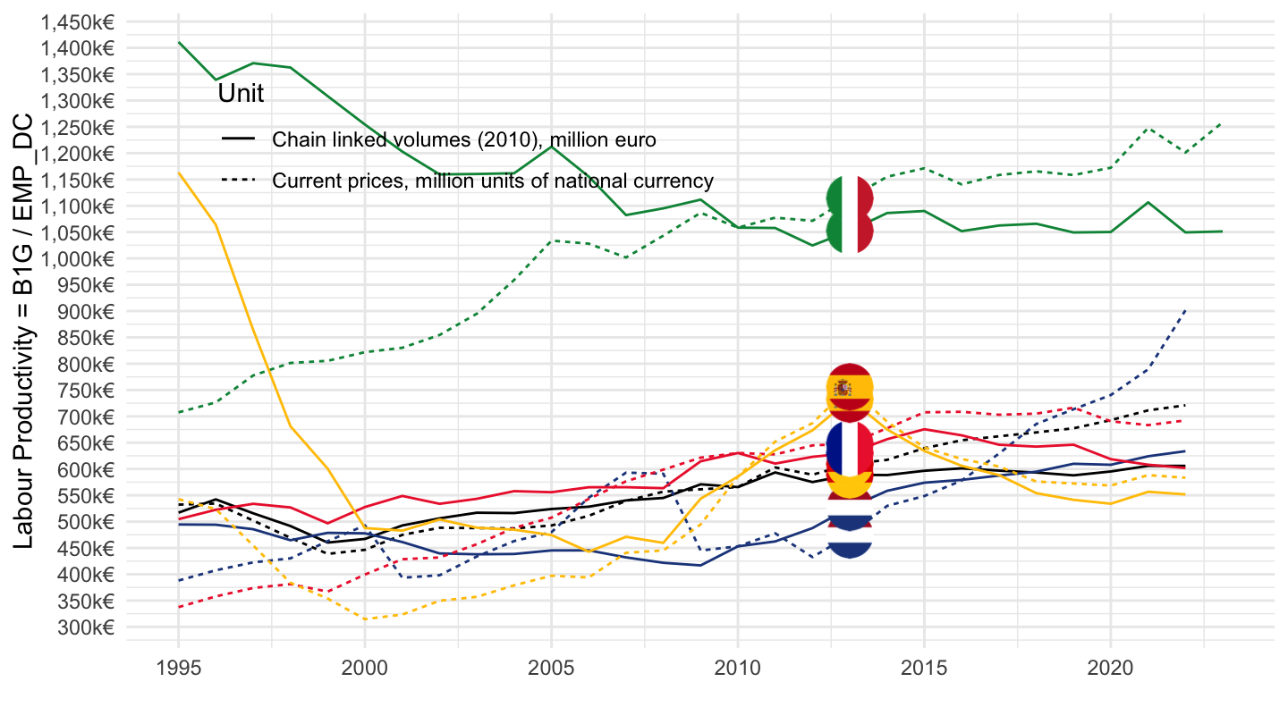
Log
Code
nama_10_a64 %>%
  filter(na_item == "B1G",
         nace_r2 %in% c("L"),
         geo %in% c("FR", "DE", "IT", "ES", "NL"),
         unit %in% c("CP_MNAC", "CLV10_MEUR")) %>%
  select_if(~ n_distinct(.) > 1) %>%
  rename(B1G = values) %>%
  left_join(nama_10_a64_e %>%
              filter(nace_r2 %in% c("L"),
                     geo %in% c("FR", "DE", "IT", "ES", "NL"),
                     unit == "THS_PER",
                     na_item == "EMP_DC") %>%
              select_if(~ n_distinct(.) > 1) %>%
              rename(EMP_DC = values), by = c("geo", "Geo", "time")) %>%
  mutate(values = B1G/EMP_DC) %>%
  year_to_date() %>%
  filter(date >= as.Date("1995-01-01")) %>%


  left_join(colors, by = c("Geo" = "country")) %>%
  mutate(color = ifelse(geo == "NL", color2, color)) %>%
  ggplot(.) + geom_line(aes(x = date, y = values, color = color, linetype = Unit)) +
  theme_minimal() + xlab("") + ylab("Labour Productivity = B1G / EMP_DC") +
  scale_color_identity() + add_flags +
  scale_x_date(breaks = seq(1960, 2100, 5) %>% paste0("-01-01") %>% as.Date,
               labels = date_format("%Y")) +
  theme(legend.position = c(0.3, 0.8)) +
  scale_y_log10(breaks = seq(0, 2000, 50),
                     labels = dollar_format(pre = "", su = "k€", acc = 1))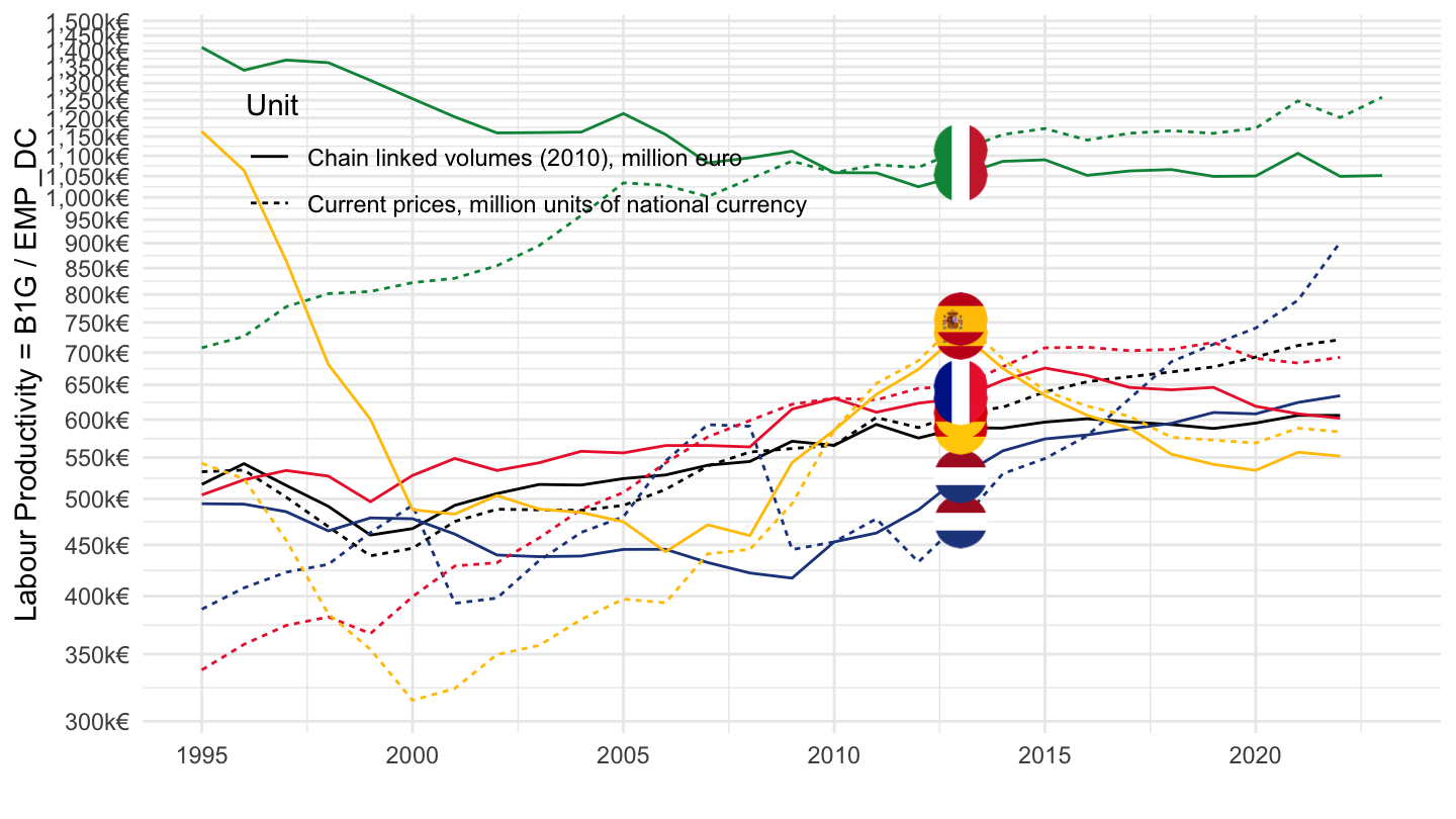
Base 100
Code
nama_10_a64 %>%
  filter(na_item == "B1G",
         nace_r2 %in% c("L"),
         geo %in% c("FR", "DE", "IT", "ES", "NL"),
         unit %in% c("CP_MNAC", "CLV10_MEUR")) %>%
  select_if(~ n_distinct(.) > 1) %>%
  rename(B1G = values) %>%
  left_join(nama_10_a64_e %>%
              filter(nace_r2 %in% c("L"),
                     geo %in% c("FR", "DE", "IT", "ES", "NL"),
                     unit == "THS_PER",
                     na_item == "EMP_DC") %>%
              select_if(~ n_distinct(.) > 1) %>%
              rename(EMP_DC = values), by = c("geo", "Geo", "time")) %>%
  mutate(values = B1G/EMP_DC) %>%
  year_to_date() %>%
  filter(date >= as.Date("1995-01-01")) %>%


  left_join(colors, by = c("Geo" = "country")) %>%
  mutate(color = ifelse(geo == "NL", color2, color)) %>%
  group_by(Geo, Unit) %>%
  arrange(date) %>%
  mutate(values = 100*values/values[1]) %>%
  ggplot(.) + geom_line(aes(x = date, y = values, color = color, linetype = Unit)) +
  theme_minimal() + xlab("") + ylab("Labour Productivity = B1G / EMP_DC") +
  scale_color_identity() + add_flags +
  scale_x_date(breaks = seq(1960, 2100, 5) %>% paste0("-01-01") %>% as.Date,
               labels = date_format("%Y")) +
  theme(legend.position = c(0.3, 0.8)) +
  scale_y_log10(breaks = seq(0, 2000, 20))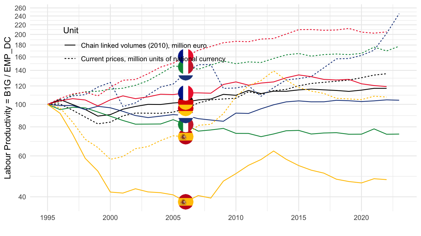
Germany, Italy, France, Spain
Table
Code
load_data("eurostat/nace_r2.RData")
nama_10_a64_e %>%
  filter(geo %in% c("FR", "DE", "IT", "ES"),
         unit == "THS_PER",
         na_item == "EMP_DC",
         time %in% c("2018")) %>%
  filter(!grepl("C", nace_r2) | nace_r2 == "TOTAL") %>%
  select(-na_item, -unit, -time) %>%


  mutate(Flag = gsub(" ", "-", str_to_lower(Geo)),
         Flag = paste0('<img src="../../bib/flags/vsmall/', Flag, '.png" alt="Flag">')) %>%
  select(nace_r2, Nace_r2, Flag, values) %>%
  group_by(Flag) %>%
  mutate(values = round(100*values/ values[nace_r2 == "TOTAL"], 1)) %>%
  filter(nace_r2 != "TOTAL")  %>%
  spread(Flag, values) %>%
  {if (is_html_output()) datatable(., filter = 'top', rownames = F, escape = F) else .}
Table - Manufacturing
Code
load_data("eurostat/nace_r2_fr.RData")
nama_10_a64_e %>%
  filter(geo %in% c("FR", "DE", "IT", "ES"),
         unit == "THS_PER",
         na_item == "EMP_DC",
         time %in% c("2018")) %>%
  filter(grepl("C", nace_r2) | nace_r2 == "TOTAL") %>%
  select(-na_item, -unit, -time) %>%


  mutate(Flag = gsub(" ", "-", str_to_lower(Geo)),
         Flag = paste0('<img src="../../bib/flags/vsmall/', Flag, '.png" alt="Flag">')) %>%
  select(nace_r2, Nace_r2, Flag, values) %>%
  group_by(Flag) %>%
  mutate(values = round(100*values/ values[nace_r2 == "TOTAL"], 1)) %>%
  filter(nace_r2 != "TOTAL")  %>%
  spread(Flag, values) %>%
  {if (is_html_output()) datatable(., filter = 'top', rownames = F, escape = F) else .}
C - Manufacturing
Persons
Code
nama_10_a64_e %>%
  filter(nace_r2 %in% c("C", "TOTAL"),
         geo %in% c("FR", "DE", "IT", "ES"),
         unit == "THS_PER",
         na_item == "EMP_DC") %>%
  year_to_date() %>%

  select(geo,  Geo, nace_r2, date, values) %>%
  spread(nace_r2, values) %>%
  mutate(values = `C`/TOTAL) %>%
  left_join(colors, by = c("Geo" = "country")) %>%
  ggplot(.) + geom_line(aes(x = date, y = values, color = color)) +
  theme_minimal() + xlab("") + ylab("Manufacturing (% of Employment)") +
  scale_color_identity() + add_4flags +
  scale_x_date(breaks = seq(1960, 2100, 5) %>% paste0("-01-01") %>% as.Date,
               labels = date_format("%Y")) +
  scale_y_continuous(breaks = 0.01*seq(-500, 200, 1),
                     labels = percent_format(accuracy = 1))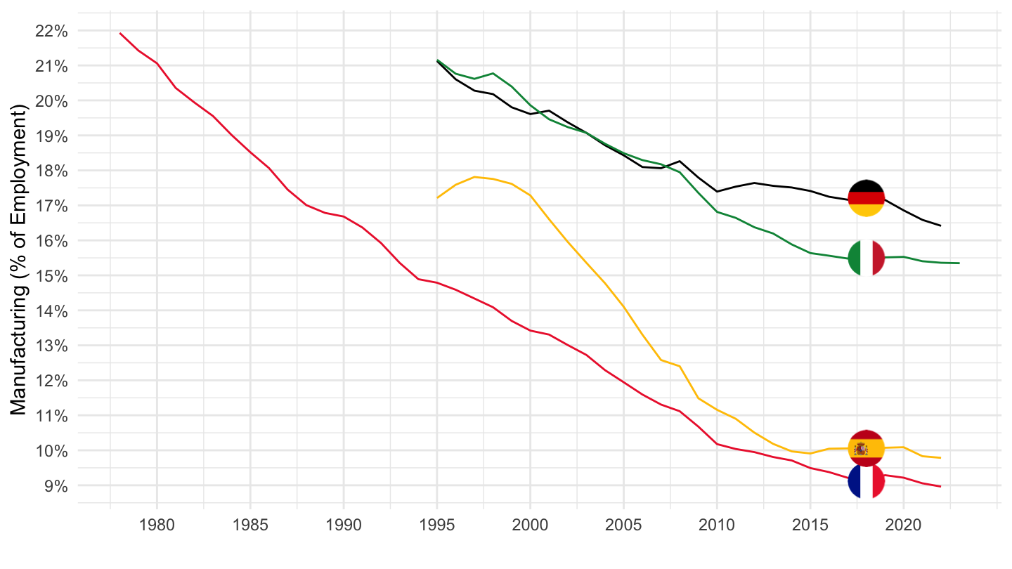
Hours worked
Code
nama_10_a64_e %>%
  filter(nace_r2 %in% c("C", "TOTAL"),
         geo %in% c("FR", "DE", "IT", "ES"),
         unit == "THS_HW",
         na_item == "EMP_DC") %>%
  year_to_date() %>%

  select(geo,  Geo, nace_r2, date, values) %>%
  spread(nace_r2, values) %>%
  mutate(values = `C`/TOTAL) %>%
  left_join(colors, by = c("Geo" = "country")) %>%
  ggplot(.) + geom_line(aes(x = date, y = values, color = color)) +
  theme_minimal() + xlab("") + ylab("Manufacturing (% of Hours worked)") +
  scale_color_identity() + add_4flags +
  scale_x_date(breaks = seq(1960, 2100, 5) %>% paste0("-01-01") %>% as.Date,
               labels = date_format("%Y")) +
  scale_y_continuous(breaks = 0.01*seq(-500, 200, 1),
                     labels = percent_format(accuracy = 1))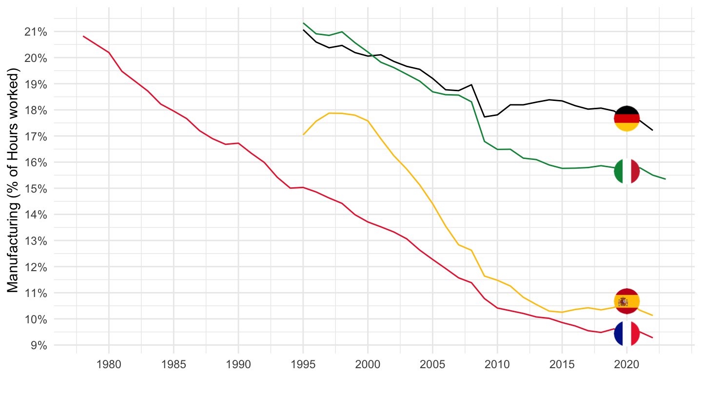
Q - Health
Persons
Code
nama_10_a64_e %>%
  filter(nace_r2 %in% c("Q", "TOTAL"),
         geo %in% c("FR", "DE", "IT", "ES"),
         unit == "THS_PER",
         na_item == "EMP_DC") %>%
  year_to_date() %>%

  select(geo,  Geo, nace_r2, date, values) %>%
  spread(nace_r2, values) %>%
  mutate(values = `Q`/TOTAL) %>%
  left_join(colors, by = c("Geo" = "country")) %>%
  ggplot(.) + geom_line(aes(x = date, y = values, color = color)) +
  theme_minimal() + xlab("") + ylab("Health (% of Employment)") +
  scale_color_identity() + add_4flags +
  scale_x_date(breaks = seq(1960, 2100, 5) %>% paste0("-01-01") %>% as.Date,
               labels = date_format("%Y")) +
  scale_y_continuous(breaks = 0.01*seq(-500, 200, 1),
                     labels = percent_format(accuracy = 1))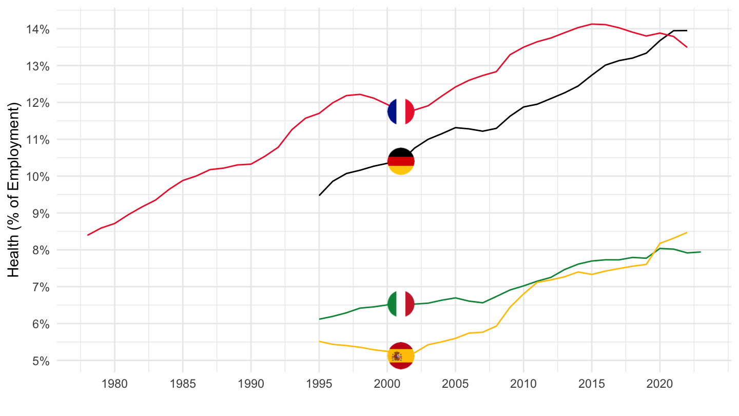
Hours worked
Code
nama_10_a64_e %>%
  filter(nace_r2 %in% c("Q", "TOTAL"),
         geo %in% c("FR", "DE", "IT", "ES"),
         unit == "THS_HW",
         na_item == "EMP_DC") %>%
  year_to_date() %>%

  select(geo,  Geo, nace_r2, date, values) %>%
  spread(nace_r2, values) %>%
  mutate(values = `Q`/TOTAL) %>%
  left_join(colors, by = c("Geo" = "country")) %>%
  ggplot(.) + geom_line(aes(x = date, y = values, color = color)) +
  theme_minimal() + xlab("") + ylab("Health (% of Hours worked)") +
  scale_color_identity() + add_4flags +
  scale_x_date(breaks = seq(1960, 2100, 5) %>% paste0("-01-01") %>% as.Date,
               labels = date_format("%Y")) +
  scale_y_continuous(breaks = 0.01*seq(-500, 200, 1),
                     labels = percent_format(accuracy = 1))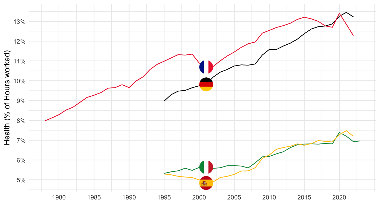
L - Real estate
Persons
Code
nama_10_a64_e %>%
  filter(nace_r2 %in% c("L", "TOTAL"),
         geo %in% c("FR", "DE", "IT", "ES"),
         unit == "THS_PER",
         na_item == "EMP_DC") %>%
  year_to_date() %>%

  select(geo,  Geo, nace_r2, date, values) %>%
  spread(nace_r2, values) %>%
  mutate(values = `L`/TOTAL) %>%
  left_join(colors, by = c("Geo" = "country")) %>%
  ggplot(.) + geom_line(aes(x = date, y = values, color = color)) +
  theme_minimal() + xlab("") + ylab("Real Estate (% of Employment)") +
  scale_color_identity() + add_4flags +
  scale_x_date(breaks = seq(1960, 2100, 5) %>% paste0("-01-01") %>% as.Date,
               labels = date_format("%Y")) +
  scale_y_continuous(breaks = 0.01*seq(-500, 200, .1),
                     labels = percent_format(accuracy = .1))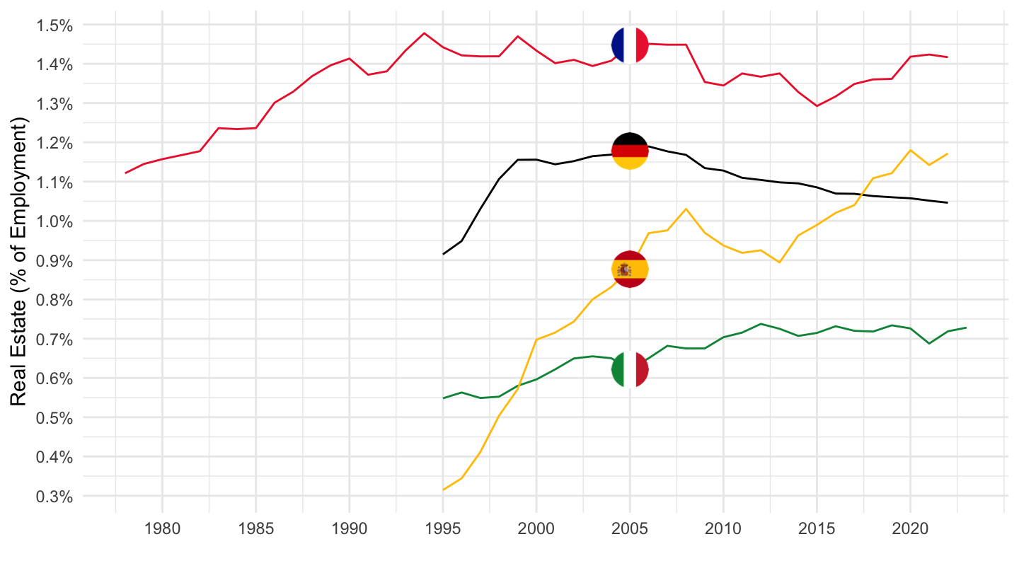
Hours worked
Code
nama_10_a64_e %>%
  filter(nace_r2 %in% c("L", "TOTAL"),
         geo %in% c("FR", "DE", "IT", "ES"),
         unit == "THS_HW",
         na_item == "EMP_DC") %>%
  year_to_date() %>%

  select(geo,  Geo, nace_r2, date, values) %>%
  spread(nace_r2, values) %>%
  mutate(values = `L`/TOTAL) %>%
  left_join(colors, by = c("Geo" = "country")) %>%
  ggplot(.) + geom_line(aes(x = date, y = values, color = color)) +
  theme_minimal() + xlab("") + ylab("Real Estate (% of Hours worked)") +
  scale_color_identity() + add_4flags +
  scale_x_date(breaks = seq(1960, 2100, 5) %>% paste0("-01-01") %>% as.Date,
               labels = date_format("%Y")) +
  scale_y_continuous(breaks = 0.01*seq(-500, 200, .1),
                     labels = percent_format(accuracy = .1))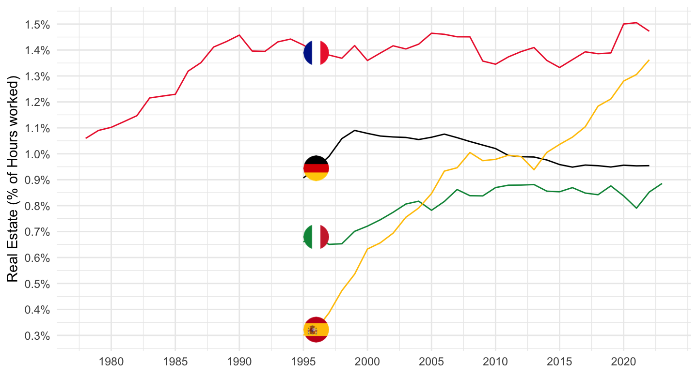
Individual Countries
France
Table
All
Code
nama_10_a64_e %>%
  filter(geo %in% c("FR"),
         unit == "THS_HW",
         na_item == "EMP_DC",
         time %in% c("1978", "1998",  "2008", "2018")) %>%

  select(nace_r2, Nace_r2, time, values) %>%
  group_by(time) %>%
  mutate(values = round(100*values/ values[nace_r2 == "TOTAL"], 1)) %>%
  filter(nace_r2 != "TOTAL")  %>%
  spread(time, values) %>%
  print_table_conditional
Manufacturing
Code
nama_10_a64_e %>%
  filter(geo %in% c("FR"),
         unit == "THS_HW",
         na_item == "EMP_DC",
         time %in% c("1978", "1998",  "2008", "2018")) %>%
  filter(grepl("C", nace_r2) | nace_r2 == "TOTAL") %>%

  select(nace_r2, Nace_r2, time, values) %>%
  group_by(time) %>%
  mutate(values = round(100*values/ values[nace_r2 == "TOTAL"], 1)) %>%
  filter(nace_r2 != "TOTAL")  %>%
  spread(time, values) %>%
  arrange(-`2018`) %>%
print_table_conditional| nace_r2 | Nace_r2 | 1978 | 1998 | 2008 | 2018 |
|---|---|---|---|---|---|
| C | Manufacturing | 22.3 | 15.1 | 11.8 | 9.9 |
| C10-C12 | Manufacture of food products; beverages and tobacco products | 2.8 | 2.7 | 2.3 | 2.3 |
| C31-C33 | Manufacture of furniture; jewellery, musical instruments, toys; repair and installation of machinery and equipment | 3.6 | 2.6 | 2.1 | 1.9 |
| C24_C25 | Manufacture of basic metals and fabricated metal products, except machinery and equipment | 3.0 | 1.9 | 1.6 | 1.3 |
| C22_C23 | Manufacture of rubber and plastic products and other non-metallic mineral products | 1.8 | 1.2 | 1.1 | 0.8 |
| C29_C30 | Manufacture of motor vehicles, trailers, semi-trailers and of other transport equipment | 2.2 | 1.2 | 1.0 | 0.8 |
| C16-C18 | Manufacture of wood, paper, printing and reproduction | 1.5 | 1.2 | 0.9 | 0.6 |
| C28 | Manufacture of machinery and equipment n.e.c. | 1.3 | 0.9 | 0.8 | 0.5 |
| C13-C15 | Manufacture of textiles, wearing apparel, leather and related products | 3.4 | 1.4 | 0.6 | 0.4 |
| C20 | Manufacture of chemicals and chemical products | 0.9 | 0.6 | 0.5 | 0.4 |
| C26 | Manufacture of computer, electronic and optical products | 0.7 | 0.6 | 0.4 | 0.3 |
| C27 | Manufacture of electrical equipment | 0.7 | 0.6 | 0.4 | 0.3 |
| C21 | Manufacture of basic pharmaceutical products and pharmaceutical preparations | 0.2 | 0.2 | 0.2 | 0.1 |
| C19 | Manufacture of coke and refined petroleum products | 0.1 | 0.0 | 0.0 | 0.0 |
Construction, Human health, Manufacturing, Real estate
All
Code
nama_10_a64_e %>%
  filter(nace_r2 %in% c("C", "TOTAL", "L", "Q", "F"),
         geo %in% c("FR"),
         unit == "THS_HW",
         na_item == "EMP_DC") %>%
  year_to_date() %>%

  select(nace_r2, Nace_r2, date, values) %>%
  group_by(date) %>%
  mutate(values = values/ values[nace_r2 == "TOTAL"]) %>%
  filter(nace_r2 != "TOTAL")  %>%
  ggplot(.) + geom_line(aes(x = date, y = values, color = Nace_r2)) +
  theme_minimal() + xlab("") + ylab("% of GDP") +
  scale_color_manual(values = viridis(5)[1:4]) +
  scale_x_date(breaks = seq(1960, 2100, 5) %>% paste0("-01-01") %>% as.Date,
               labels = date_format("%Y")) +
  scale_y_continuous(breaks = 0.01*seq(-500, 200, 1),
                     labels = percent_format(accuracy = 1)) +
  theme(legend.position = c(0.75, 0.85),
        legend.title = element_blank())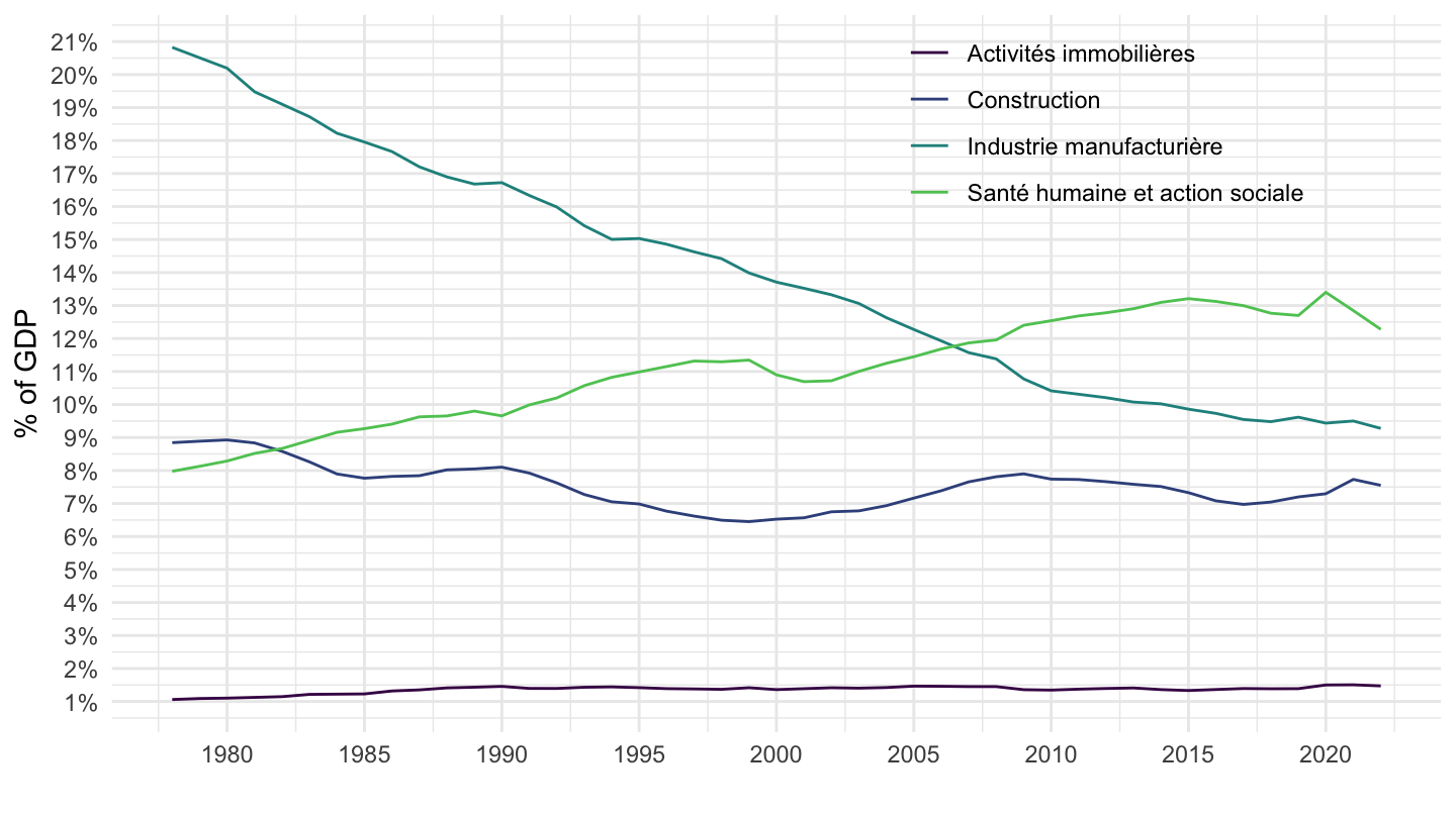
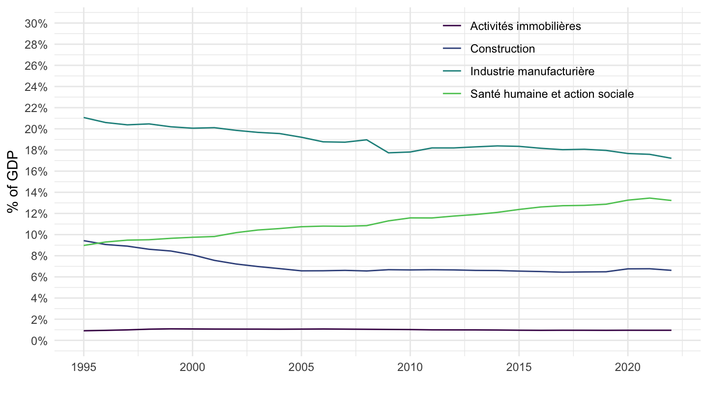
1995-
Code
nama_10_a64_e %>%
  filter(nace_r2 %in% c("C", "TOTAL", "L", "Q", "F"),
         geo %in% c("FR"),
         unit == "THS_HW",
         na_item == "EMP_DC") %>%
  year_to_date() %>%
  filter(date >= as.Date("1995-01-01")) %>%

  select(nace_r2, Nace_r2, date, values) %>%
  group_by(date) %>%
  mutate(values = values/ values[nace_r2 == "TOTAL"]) %>%
  filter(nace_r2 != "TOTAL")  %>%
  ggplot(.) + geom_line(aes(x = date, y = values, color = Nace_r2)) +
  theme_minimal() + xlab("") + ylab("% of GDP") +
  scale_color_manual(values = viridis(5)[1:4]) +
  scale_x_date(breaks = seq(1960, 2100, 5) %>% paste0("-01-01") %>% as.Date,
               labels = date_format("%Y")) +
  scale_y_continuous(breaks = 0.01*seq(0, 30, 2),
                     labels = percent_format(accuracy = 1),
                     limits = c(0, 0.3)) +
  theme(legend.position = c(0.75, 0.85),
        legend.title = element_blank())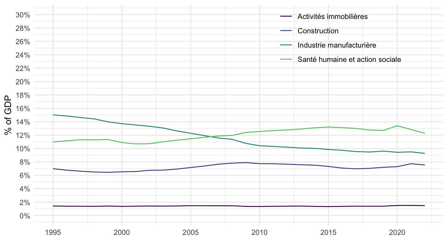
Germany
Table
All
Code
nama_10_a64_e %>%
  filter(geo %in% c("DE"),
         unit == "THS_HW",
         na_item == "EMP_DC",
         time %in% c("1978", "1998",  "2008", "2018")) %>%

  select(nace_r2, Nace_r2, time, values) %>%
  group_by(time) %>%
  mutate(values = round(100*values/ values[nace_r2 == "TOTAL"], 1)) %>%
  filter(nace_r2 != "TOTAL")  %>%
  spread(time, values) %>%
  print_table_conditional
Manufacturing
Code
nama_10_a64_e %>%
  filter(geo %in% c("DE"),
         unit == "THS_HW",
         na_item == "EMP_DC",
         time %in% c("1978", "1998",  "2008", "2018")) %>%
  filter(grepl("C", nace_r2) | nace_r2 == "TOTAL") %>%

  select(nace_r2, Nace_r2, time, values) %>%
  group_by(time) %>%
  mutate(values = round(100*values/ values[nace_r2 == "TOTAL"], 1)) %>%
  filter(nace_r2 != "TOTAL")  %>%
  spread(time, values) %>%
  arrange(-`2018`) %>%
print_table_conditional| nace_r2 | Nace_r2 | 1998 | 2008 | 2018 |
|---|---|---|---|---|
| C | Manufacturing | 20.5 | 19.0 | 18.1 |
| C24_C25 | Manufacture of basic metals and fabricated metal products, except machinery and equipment | 3.1 | 3.0 | 2.9 |
| C28 | Manufacture of machinery and equipment n.e.c. | 2.8 | 2.8 | 2.8 |
| C29_C30 | Manufacture of motor vehicles, trailers, semi-trailers and of other transport equipment | 2.5 | 2.4 | 2.4 |
| C10-C12 | Manufacture of food products; beverages and tobacco products | 2.3 | 2.3 | 2.1 |
| C22_C23 | Manufacture of rubber and plastic products and other non-metallic mineral products | 1.9 | 1.7 | 1.7 |
| C31-C33 | Manufacture of furniture; jewellery, musical instruments, toys; repair and installation of machinery and equipment | 1.8 | 1.6 | 1.6 |
| C27 | Manufacture of electrical equipment | 1.4 | 1.3 | 1.2 |
| C16-C18 | Manufacture of wood, paper, printing and reproduction | 1.7 | 1.3 | 1.0 |
| C20 | Manufacture of chemicals and chemical products | 1.0 | 0.9 | 0.9 |
| C26 | Manufacture of computer, electronic and optical products | 0.9 | 0.9 | 0.9 |
| C13-C15 | Manufacture of textiles, wearing apparel, leather and related products | 0.7 | 0.4 | 0.3 |
| C21 | Manufacture of basic pharmaceutical products and pharmaceutical preparations | 0.3 | 0.3 | 0.3 |
| C19 | Manufacture of coke and refined petroleum products | 0.1 | 0.0 | 0.0 |
Construction, Human health, Manufacturing, Real estate
Code
nama_10_a64_e %>%
  filter(nace_r2 %in% c("C", "TOTAL", "L", "Q", "F"),
         geo %in% c("DE"),
         unit == "THS_HW",
         na_item == "EMP_DC") %>%
  year_to_date() %>%

  select(nace_r2, Nace_r2, date, values) %>%
  group_by(date) %>%
  mutate(values = values/ values[nace_r2 == "TOTAL"]) %>%
  filter(nace_r2 != "TOTAL")  %>%
  ggplot(.) + geom_line(aes(x = date, y = values, color = Nace_r2)) +
  theme_minimal() + xlab("") + ylab("% of GDP") +
  scale_color_manual(values = viridis(5)[1:4]) +
  scale_x_date(breaks = seq(1960, 2100, 5) %>% paste0("-01-01") %>% as.Date,
               labels = date_format("%Y")) +
  scale_y_continuous(breaks = 0.01*seq(0, 30, 2),
                     labels = percent_format(accuracy = 1),
                     limits = c(0, 0.3)) +
  theme(legend.position = c(0.75, 0.85),
        legend.title = element_blank())