GDP and main components (output, expenditure and income)
Data - Eurostat
Info
Last observation: Annual: 2025 (N = 33,024)
First observation: Annual: 1975 (N = 1,402)
Last data update: 23 jul 2026, 22:29. Last compile: 24 jul 2026, 02:46
Structure
Latest GDP Numbers
2019, 2020 Values
Code
nama_10_gdp %>%
  filter(unit == "CP_MEUR",
         na_item == "B1GQ",
         time %in% c("2019", "2020")) %>%

  select(time, geo, Geo, values) %>%
  spread(time, values) %>%
  mutate(Geo = ifelse(geo == "DE", "Germany", Geo)) %>%
  mutate(Flag = gsub(" ", "-", str_to_lower(Geo)),
         Flag = paste0('<img src="../../bib/flags/vsmall/', Flag, '.png" alt="Flag">')) %>%
  select(Flag, everything()) %>%
  {if (is_html_output()) datatable(., filter = 'top', rownames = F, escape = F) else .}
2019, 2020 % increase
Code
nama_10_gdp %>%
  filter(unit == "CLV_PCH_PRE",
         na_item == "B1GQ",
         time %in% c("2019", "2020")) %>%

  select(time, geo, Geo, values) %>%
  spread(time, values) %>%
  mutate(Geo = ifelse(geo == "DE", "Germany", Geo)) %>%
  mutate(Flag = gsub(" ", "-", str_to_lower(Geo)),
         Flag = paste0('<img src="../../bib/flags/vsmall/', Flag, '.png" alt="Flag">')) %>%
  select(Flag, everything()) %>%
  arrange(`2020`) %>%
  {if (is_html_output()) datatable(., filter = 'top', rownames = F, escape = F) else .}
2019, 2020 All Units
Code
nama_10_gdp %>%
  filter(na_item == "B1GQ",
         time %in% c("2020")) %>%

  select(unit, geo, Geo, values) %>%
  spread(unit, values) %>%
  mutate(Geo = ifelse(geo == "DE", "Germany", Geo)) %>%
  mutate(Flag = gsub(" ", "-", str_to_lower(Geo)),
         Flag = paste0('<img src="../../bib/flags/vsmall/', Flag, '.png" alt="Flag">')) %>%
  select(Flag, everything()) %>%
  {if (is_html_output()) datatable(., filter = 'top', rownames = F, escape = F) else .}
France, Germany, Italy, UK
Billions
Code
nama_10_gdp %>%
  filter(unit == "CP_MEUR",
         time == "2019",
         geo %in% c("FR", "DE", "IT", "UK")) %>%

  mutate(Geo = ifelse(geo == "DE", "Germany", Geo)) %>%
  select(-geo) %>%
  mutate(Geo = gsub(" ", "-", str_to_lower(Geo)),
         Geo = paste0('<img src="../../bib/flags/vsmall/', Geo, '.png" alt="Flag">')) %>%
  spread(Geo, values) %>%
  {if (is_html_output()) datatable(., filter = 'top', rownames = F, escape = F) else .}
% of GDP
Code
nama_10_gdp %>%
  filter(unit == "PC_GDP",
         time == "2019",
         geo %in% c("FR", "DE", "IT", "UK")) %>%

  mutate(Geo = ifelse(geo == "DE", "Germany", Geo)) %>%
  select(-geo) %>%
  mutate(Geo = gsub(" ", "-", str_to_lower(Geo)),
         Geo = paste0('<img src="../../bib/flags/vsmall/', Geo, '.png" alt="Flag">')) %>%
  spread(Geo, values) %>%
  {if (is_html_output()) datatable(., filter = 'top', rownames = F, escape = F) else .}
Operating Surplus and Mixed Income / GDP (B1G)
Table
Code
nama_10_gdp %>%
  filter(na_item %in% c("B2A3G"),
         unit == "PC_GDP",
         time %in% c("1989", "1999", "2009", "2019")) %>%
  select(time, geo, Geo, values) %>%

  spread(time, values) %>%
  mutate(Geo = ifelse(geo == "DE", "Germany", Geo)) %>%
  mutate(Flag = gsub(" ", "-", str_to_lower(Geo)),
         Flag = paste0('<img src="../../bib/flags/vsmall/', Flag, '.png" alt="Flag">')) %>%
  select(Flag, everything()) %>%
  {if (is_html_output()) datatable(., filter = 'top', rownames = F, escape = F) else .}
Net Exports
Table
Code
nama_10_gdp %>%
  filter(na_item %in% c("P6", "P7"),
         unit == "PC_GDP",
         time %in% c("1989", "1999", "2009", "2019")) %>%
  spread(na_item, values) %>%
  mutate(NX = P6 - P7) %>%
  select(-P6, -P7) %>%
  mutate(NX = round(as.numeric(NX), 1)) %>%
  spread(time, NX) %>%
  mutate(Geo = ifelse(geo == "DE", "Germany", Geo)) %>%
  mutate(Flag = gsub(" ", "-", str_to_lower(Geo)),
         Flag = paste0('<img src="../../bib/flags/vsmall/', Flag, '.png" alt="Flag">')) %>%
  select(Flag, everything()) %>%
  {if (is_html_output()) datatable(., filter = 'top', rownames = F, escape = F) else .}
Greece, Portugal, Spain
Code
nama_10_gdp %>%
  filter(na_item %in% c("P6", "P7"),
         unit == "PC_GDP",
         geo %in% c("EL", "ES", "PT")) %>%
  year_to_date %>%
  select(geo, Geo, date, na_item, values) %>%
  mutate(Geo= ifelse(geo == "EA20", "Europe", Geo)) %>%
  spread(na_item, values) %>%
  mutate(values = (P6 - P7)/100) %>%
  left_join(colors, by = c("Geo" = "country")) %>%
  ggplot + geom_line(aes(x = date, y = values, color = color)) +
  scale_color_identity() + theme_minimal()  + add_3flags +
  scale_x_date(breaks = as.Date(paste0(seq(1960, 2100, 5), "-01-01")),
               labels = date_format("%Y")) +
  xlab("") + ylab("Net Exports (% of GDP)") +
  scale_y_continuous(breaks = 0.01*seq(-30, 30, 1),
                labels = percent_format(a = 1)) +
  geom_hline(yintercept = 0, linetype = "dashed",  color = "black")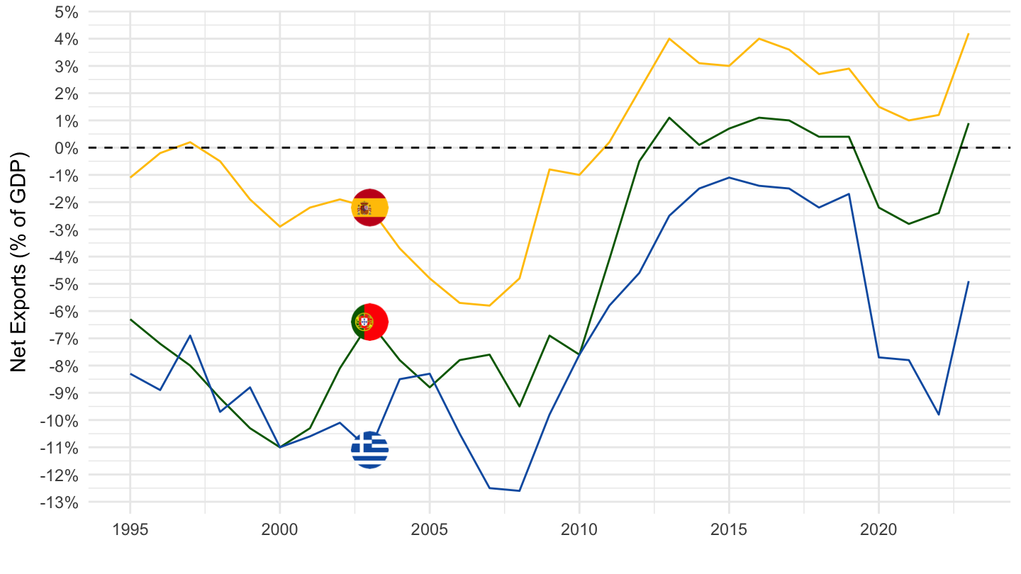
Germany, France, Eurozone
Code
nama_10_gdp %>%
  filter(na_item %in% c("P6", "P7"),
         unit == "PC_GDP",
         geo %in% c("FR", "DE", "EA20")) %>%
  select(time, na_item, geo, Geo, values) %>%
  year_to_date %>%

  mutate(Geo= ifelse(geo == "EA20", "Europe", Geo)) %>%
  spread(na_item, values) %>%
  mutate(values = (P6 - P7)/100) %>%
  left_join(colors, by = c("Geo" = "country")) %>%
  ggplot + geom_line(aes(x = date, y = values, color = color)) +
  scale_color_identity() + theme_minimal()  + add_3flags +
  scale_x_date(breaks = as.Date(paste0(seq(1960, 2100, 5), "-01-01")),
               labels = date_format("%Y")) +
  xlab("") + ylab("Net Exports (% of GDP)") +
  scale_y_continuous(breaks = 0.01*seq(-30, 30, 1),
                labels = percent_format(a = 1)) +
  geom_hline(yintercept = 0, linetype = "dashed",  color = "black")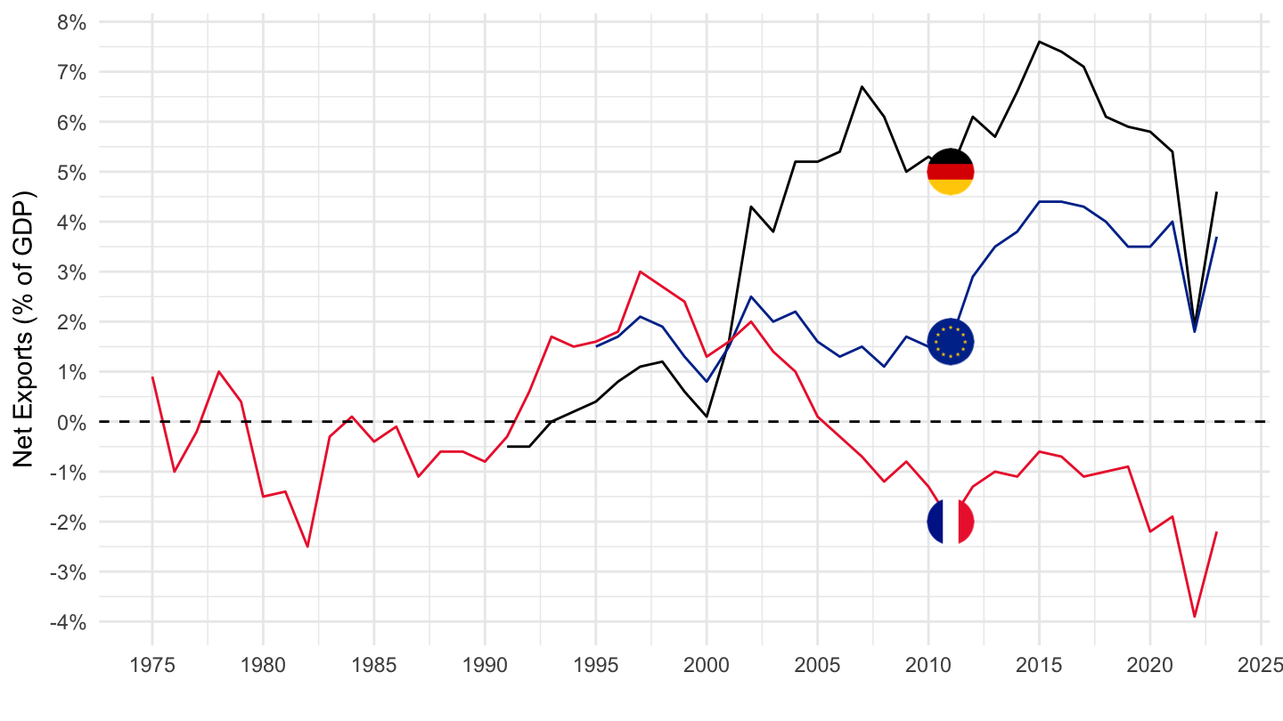
Germany, France, Italy, Eurozone
Code
nama_10_gdp %>%
  filter(na_item %in% c("P6", "P7"),
         unit == "PC_GDP",
         geo %in% c("FR", "DE", "IT", "EA20")) %>%
  select(time, na_item, geo, Geo, values) %>%
  year_to_date %>%

  mutate(Geo= ifelse(geo == "EA20", "Europe", Geo)) %>%
  spread(na_item, values) %>%
  mutate(values = (P6 - P7)/100) %>%
  left_join(colors, by = c("Geo" = "country")) %>%
  filter(date >= as.Date("1995-01-01")) %>%
  ggplot + geom_line(aes(x = date, y = values, color = color)) +
  scale_color_identity() + theme_minimal()  + add_4flags +
  scale_x_date(breaks = as.Date(paste0(seq(1960, 2100, 2), "-01-01")),
               labels = date_format("%Y")) +
  xlab("") + ylab("Net Exports (% of GDP)") +
  scale_y_continuous(breaks = 0.01*seq(-30, 30, 1),
                labels = percent_format(a = 1)) +
  geom_hline(yintercept = 0, linetype = "dashed",  color = "black")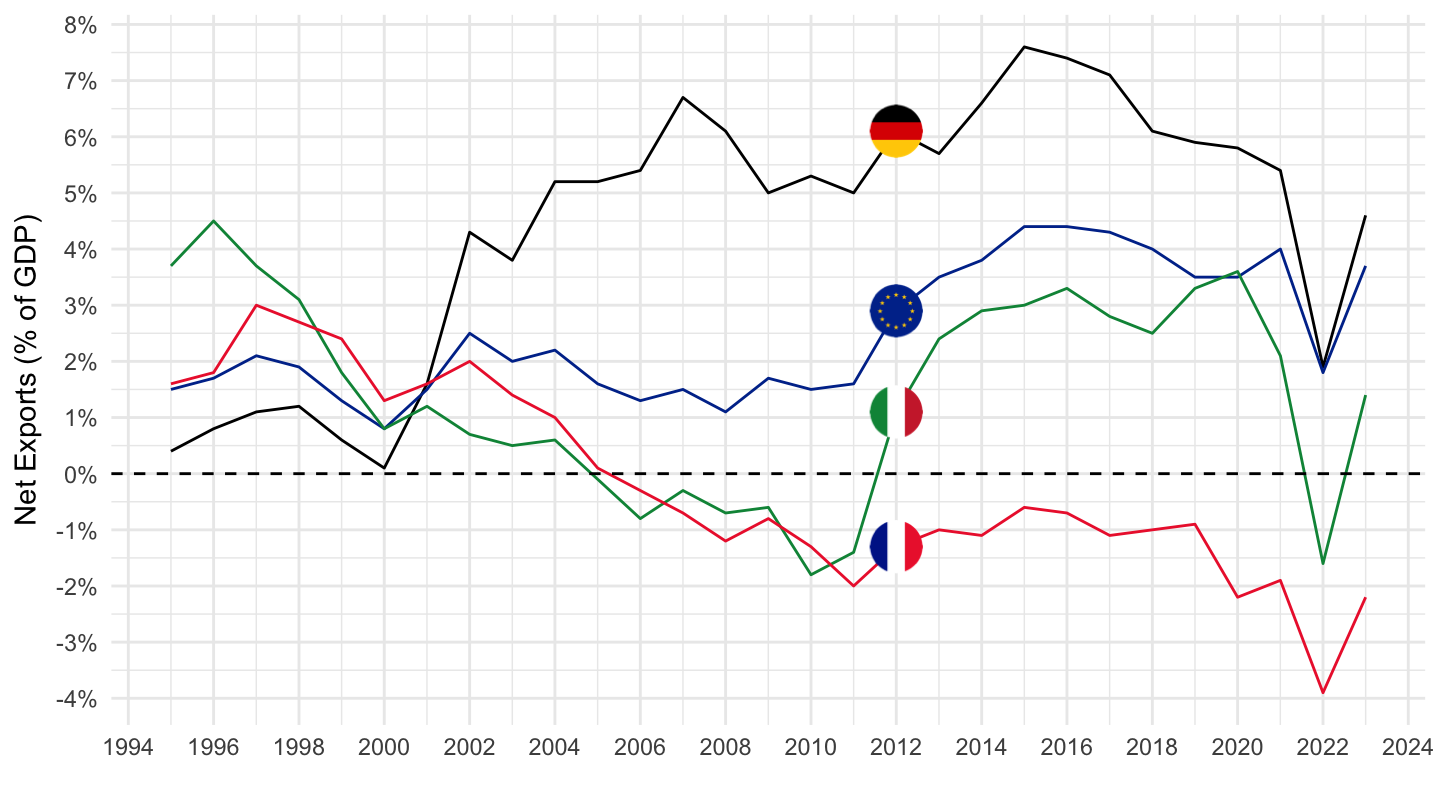
Germany, France, Eurozone, Netherlands
All
Code
nama_10_gdp %>%
  filter(na_item %in% c("P6", "P7"),
         unit == "PC_GDP",
         geo %in% c("FR", "DE", "EA20", "NL")) %>%
  select(time, na_item, geo, Geo, values) %>%
  year_to_date %>%

  mutate(Geo= ifelse(geo == "EA20", "Europe", Geo)) %>%
  spread(na_item, values) %>%
  mutate(values = (P6 - P7)/100) %>%
  left_join(colors, by = c("Geo" = "country")) %>%
  ggplot + geom_line(aes(x = date, y = values, color = color)) +
  scale_color_identity() + theme_minimal()  + add_4flags +
  scale_x_date(breaks = as.Date(paste0(seq(1960, 2100, 5), "-01-01")),
               labels = date_format("%Y")) +
  xlab("") + ylab("Net Exports (% of GDP)") +
  scale_y_continuous(breaks = 0.01*seq(-30, 30, 1),
                labels = percent_format(a = 1)) +
  geom_hline(yintercept = 0, linetype = "dashed",  color = "black")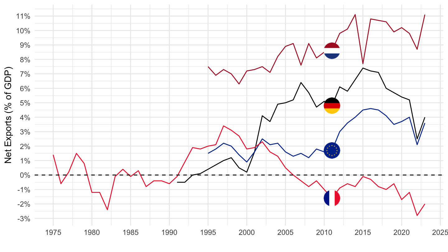
1995-
Code
nama_10_gdp %>%
  filter(na_item %in% c("P6", "P7"),
         unit == "PC_GDP",
         geo %in% c("FR", "DE", "EA20", "NL")) %>%
  select(time, na_item, geo, Geo, values) %>%
  year_to_date %>%
  filter(date >= as.Date("1995-01-01")) %>%

  mutate(Geo= ifelse(geo == "EA20", "Europe", Geo)) %>%
  spread(na_item, values) %>%
  mutate(values = (P6 - P7)/100) %>%
  left_join(colors, by = c("Geo" = "country")) %>%
  ggplot + geom_line(aes(x = date, y = values, color = color)) +
  scale_color_identity() + theme_minimal()  + add_4flags +
  scale_x_date(breaks = as.Date(paste0(seq(1960, 2100, 5), "-01-01")),
               labels = date_format("%Y")) +
  xlab("") + ylab("Net Exports (% of GDP)") +
  scale_y_continuous(breaks = 0.01*seq(-30, 30, 1),
                labels = percent_format(a = 1)) +
  geom_hline(yintercept = 0, linetype = "dashed",  color = "black")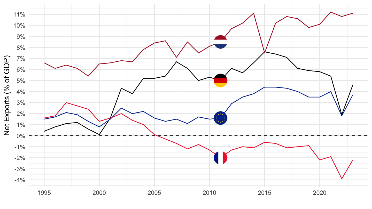
Germany, France, Italy
Code
nama_10_gdp %>%
  filter(na_item %in% c("P6", "P7"),
         unit == "PC_GDP",
         geo %in% c("FR", "DE", "IT")) %>%
  select(time, na_item, geo, Geo, values) %>%
  year_to_date %>%

  spread(na_item, values) %>%
  mutate(values = (P6 - P7)/100) %>%
  left_join(colors, by = c("Geo" = "country")) %>%
  ggplot + geom_line(aes(x = date, y = values, color = color)) +
  scale_color_identity() + theme_minimal()  + add_3flags +
  scale_x_date(breaks = as.Date(paste0(seq(1960, 2100, 5), "-01-01")),
               labels = date_format("%Y")) +
  xlab("") + ylab("Net Exports (% of GDP)") +
  scale_y_continuous(breaks = 0.01*seq(-30, 30, 1),
                labels = percent_format(a = 1)) +
  geom_hline(yintercept = 0, linetype = "dashed",  color = "black")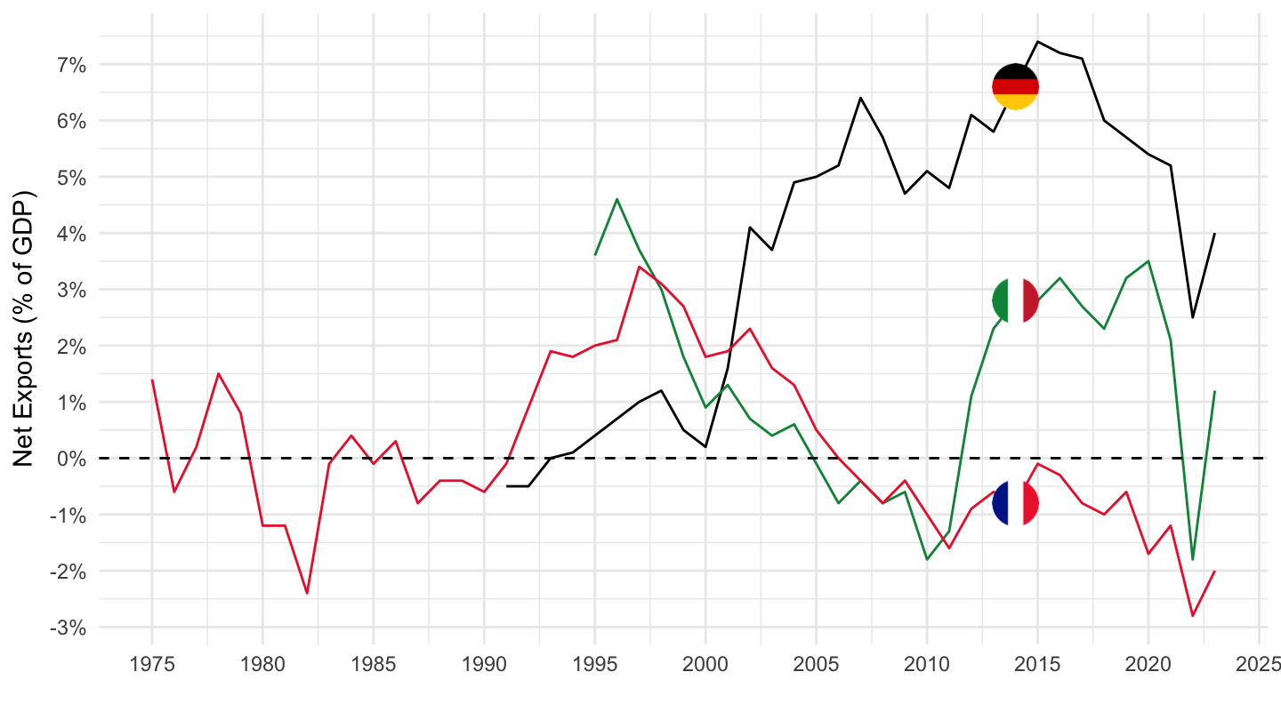
Poland, France, Italy
Code
nama_10_gdp %>%
  filter(na_item %in% c("P6", "P7"),
         unit == "PC_GDP",
         geo %in% c("PL", "DE", "IT")) %>%
  select(time, na_item, geo, Geo, values) %>%
  year_to_date %>%

  spread(na_item, values) %>%
  mutate(values = (P6 - P7)/100) %>%
  left_join(colors, by = c("Geo" = "country")) %>%
  ggplot + geom_line(aes(x = date, y = values, color = color)) +
  scale_color_identity() + theme_minimal()  + add_3flags +
  scale_x_date(breaks = as.Date(paste0(seq(1960, 2100, 5), "-01-01")),
               labels = date_format("%Y")) +
  xlab("") + ylab("Net Exports (% of GDP)") +
  scale_y_continuous(breaks = 0.01*seq(-30, 30, 1),
                labels = percent_format(a = 1)) +
  geom_hline(yintercept = 0, linetype = "dashed",  color = "black")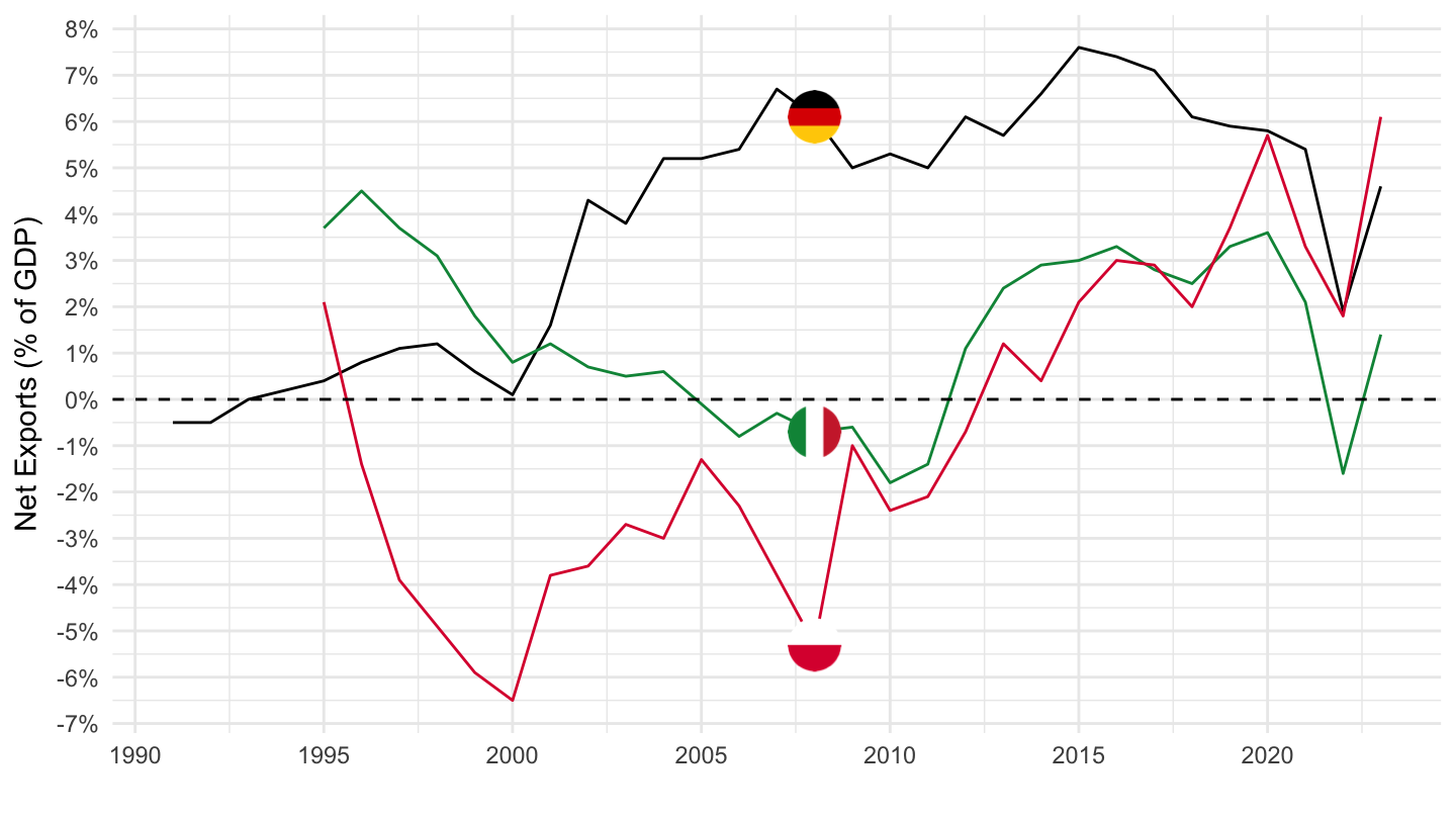
Pologne, Hongrie, Slovénie
Code
nama_10_gdp %>%
  filter(na_item %in% c("P6", "P7"),
         unit == "PC_GDP",
         geo %in% c("PL", "HU", "SI")) %>%
  select(time, na_item, geo, Geo, values) %>%
  year_to_date %>%

  spread(na_item, values) %>%
  mutate(values = (P6 - P7)/100) %>%
  left_join(colors, by = c("Geo" = "country")) %>%
  ggplot + geom_line(aes(x = date, y = values, color = color)) +
  scale_color_identity() + theme_minimal()  + add_3flags +
  scale_x_date(breaks = as.Date(paste0(seq(1960, 2100, 5), "-01-01")),
               labels = date_format("%Y")) +
  xlab("") + ylab("Net Exports (% of GDP)") +
  scale_y_continuous(breaks = 0.01*seq(-30, 30, 1),
                labels = percent_format(a = 1)) +
  geom_hline(yintercept = 0, linetype = "dashed",  color = "black")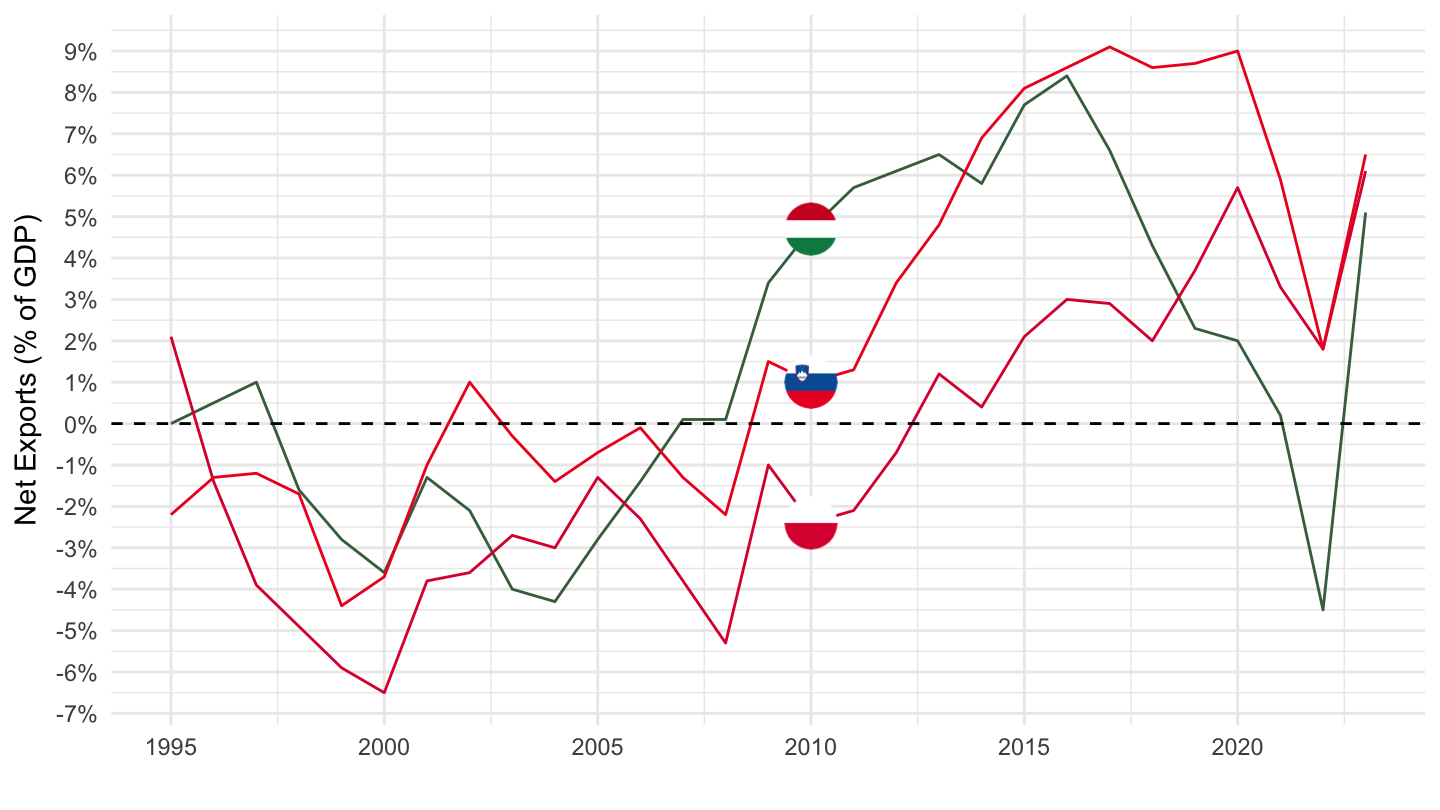
Poland, Austria, Germany, Tchequia, Hungary, Slovakia
All
Code
nama_10_gdp %>%
  filter(na_item %in% c("P6", "P7"),
         unit == "PC_GDP",
         geo %in% c("PL", "DE", "SK", "CZ", "HU", "AT")) %>%
  select(time, na_item, geo, Geo, values) %>%
  year_to_date %>%

  spread(na_item, values) %>%
  mutate(values = (P6 - P7)/100) %>%
  left_join(colors, by = c("Geo" = "country")) %>%
  ggplot + geom_line(aes(x = date, y = values, color = color)) +
  scale_color_identity() + theme_minimal()  + add_6flags +
  scale_x_date(breaks = as.Date(paste0(seq(1960, 2100, 5), "-01-01")),
               labels = date_format("%Y")) +
  xlab("") + ylab("Net Exports (% of GDP)") +
  scale_y_continuous(breaks = 0.01*seq(-30, 30, 1),
                labels = percent_format(a = 1)) +
  geom_hline(yintercept = 0, linetype = "dashed",  color = "black")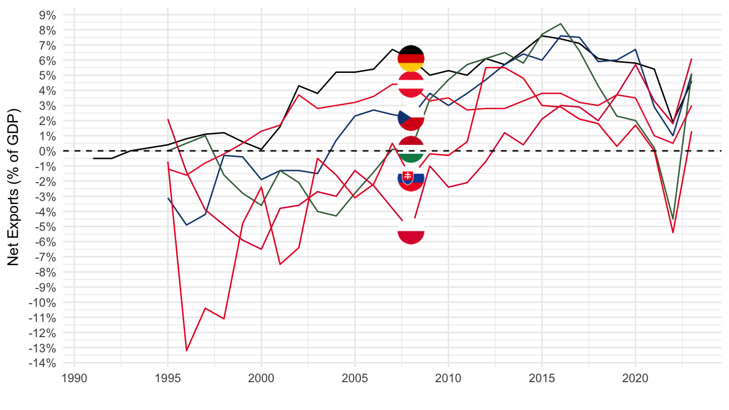
2000-
Code
nama_10_gdp %>%
  filter(na_item %in% c("P6", "P7"),
         unit == "PC_GDP",
         geo %in% c("PL", "DE", "SK", "CZ", "HU", "AT")) %>%
  select(time, na_item, geo, Geo, values) %>%
  year_to_date %>%
  filter(date >= as.Date("2000-01-01")) %>%

  spread(na_item, values) %>%
  mutate(values = (P6 - P7)/100) %>%
  left_join(colors, by = c("Geo" = "country")) %>%
  ggplot + geom_line(aes(x = date, y = values, color = color)) +
  scale_color_identity() + theme_minimal()  + add_6flags +
  scale_x_date(breaks = as.Date(paste0(seq(1960, 2100, 5), "-01-01")),
               labels = date_format("%Y")) +
  xlab("") + ylab("Net Exports (% of GDP)") +
  scale_y_continuous(breaks = 0.01*seq(-30, 30, 1),
                labels = percent_format(a = 1)) +
  geom_hline(yintercept = 0, linetype = "dashed",  color = "black")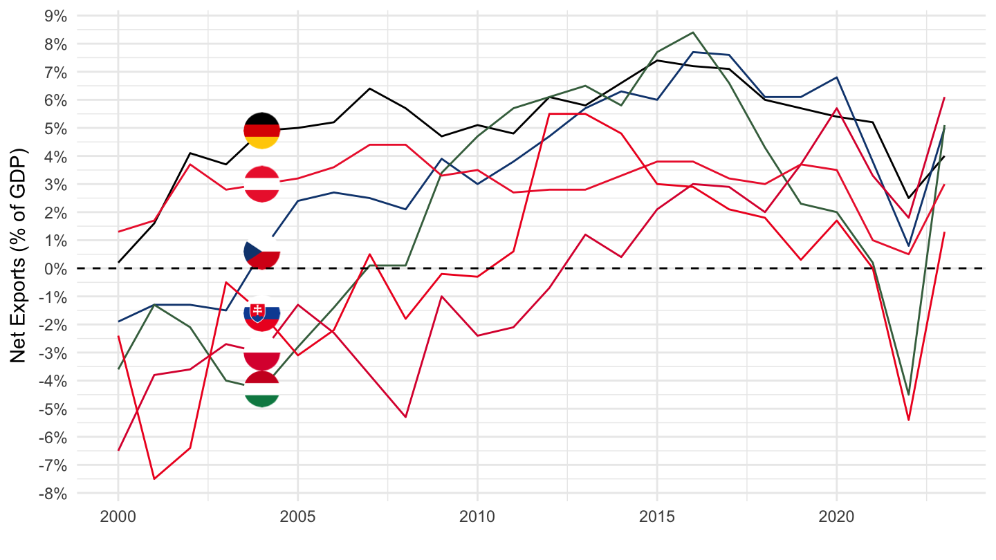
United Kingdom, Portugal, Finland, Romania, France, Greece, Sweden
Code
nama_10_gdp %>%
  filter(na_item %in% c("P6", "P7"),
         unit == "PC_GDP",
         geo %in% c("UK", "PT", "FI", "RO", "FR", "EL", "SE")) %>%
  select(time, na_item, geo, Geo, values) %>%
  year_to_date %>%
  filter(date >= as.Date("2000-01-01")) %>%

  spread(na_item, values) %>%
  mutate(values = (P6 - P7)/100) %>%
  left_join(colors, by = c("Geo" = "country")) %>%
  ggplot + geom_line(aes(x = date, y = values, color = color)) +
  scale_color_identity() + theme_minimal()  + add_7flags +
  scale_x_date(breaks = as.Date(paste0(seq(1960, 2100, 5), "-01-01")),
               labels = date_format("%Y")) +
  xlab("") + ylab("Net Exports (% of GDP)") +
  scale_y_continuous(breaks = 0.01*seq(-30, 30, 1),
                labels = percent_format(a = 1)) +
  geom_hline(yintercept = 0, linetype = "dashed",  color = "black")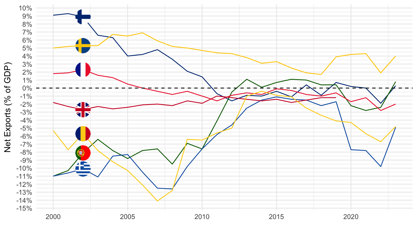
Gross Domestic Product
Table
Code
nama_10_gdp %>%
  filter(time %in% c("2020", "2019", "2000"),
         # B1GQ: Gross domestic product at market prices
         na_item == "B1GQ",
         unit == "CLV10_MEUR") %>%

  select(geo, Geo, time, values) %>%
  spread(time, values) %>%
  print_table_conditional()
France, Germany, Italy
All
Code
nama_10_gdp %>%
  filter(geo %in% c("FR", "DE", "IT"),
         # B1GQ: Gross domestic product at market prices
         na_item == "B1GQ",
         unit == "CLV10_MEUR") %>%

  year_to_date %>%
  mutate(values = values/1000) %>%
  left_join(colors, by = c("Geo" = "country")) %>%
  ggplot + geom_line(aes(x = date, y = values, color = color)) +
  scale_color_identity() + add_3flags + theme_minimal()  +
  scale_x_date(breaks = as.Date(paste0(seq(1960, 2100, 5), "-01-01")),
               labels = date_format("%Y")) +
  xlab("") + ylab("") +
  scale_y_log10(breaks = seq(0, 3000, 100),
                labels = dollar_format(suffix = " Bn€", prefix = "", accuracy = 1))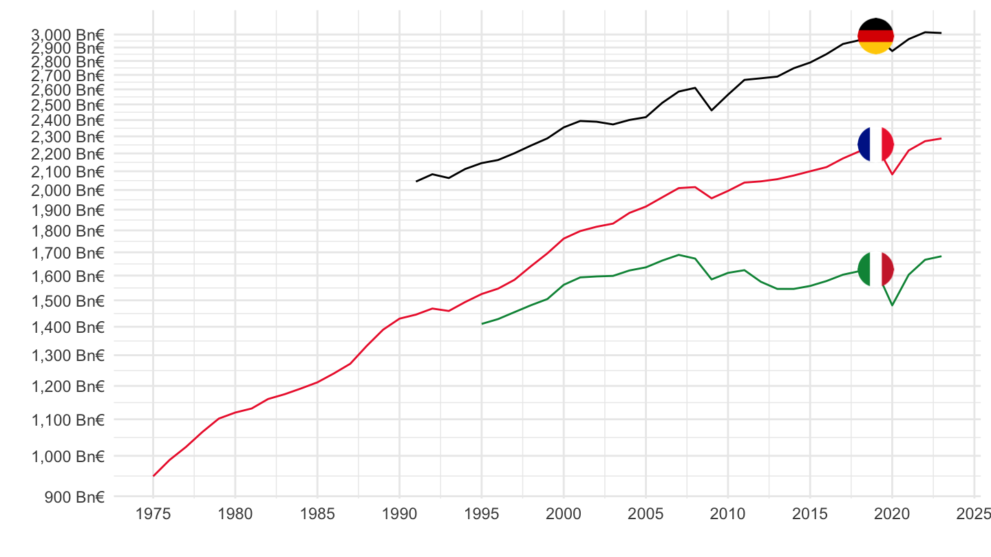
1995-
Code
nama_10_gdp %>%
  filter(geo %in% c("FR", "DE", "IT"),
         na_item == "B1GQ",
         unit == "CLV10_MEUR") %>%

  year_to_date %>%
  mutate(values = values/1000) %>%
  filter(date >= as.Date("1995-01-01")) %>%
  left_join(colors, by = c("Geo" = "country")) %>%
  ggplot + geom_line(aes(x = date, y = values, color = color)) +
  scale_color_identity() + add_3flags + theme_minimal()  +
  scale_x_date(breaks = as.Date(paste0(seq(1960, 2100, 5), "-01-01")),
               labels = date_format("%Y")) +
  xlab("") + ylab("") +
  scale_y_log10(breaks = seq(0, 3000, 100),
                labels = dollar_format(suffix = " Bn€", prefix = "", accuracy = 1))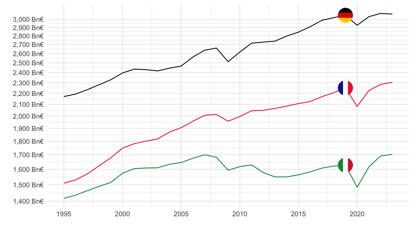
France, Germany, Eurozone, Italy, Spain
1995-
Valeur
Code
nama_10_gdp %>%
  filter(geo %in% c("FR", "DE", "EA20", "IT", "ES"),
         # B1GQ: Gross domestic product at market prices
         na_item == "B1GQ",
         unit == "CLV10_MEUR") %>%

  year_to_date %>%
  mutate(values = values/1000) %>%
  filter(date >= as.Date("1995-01-01")) %>%
  mutate(Geo = ifelse(geo == "EA20", "Europe", Geo)) %>%
  left_join(colors, by = c("Geo" = "country")) %>%
  ggplot + geom_line(aes(x = date, y = values, color = color)) +
  scale_color_identity() + add_5flags + theme_minimal()  +
  scale_x_date(breaks = as.Date(paste0(seq(1960, 2100, 5), "-01-01")),
               labels = date_format("%Y")) +
  xlab("") + ylab("") +
  scale_y_log10(breaks = seq(1000, 15000, 1000),
                labels = dollar_format(suffix = " Bn€", prefix = "", accuracy = 1))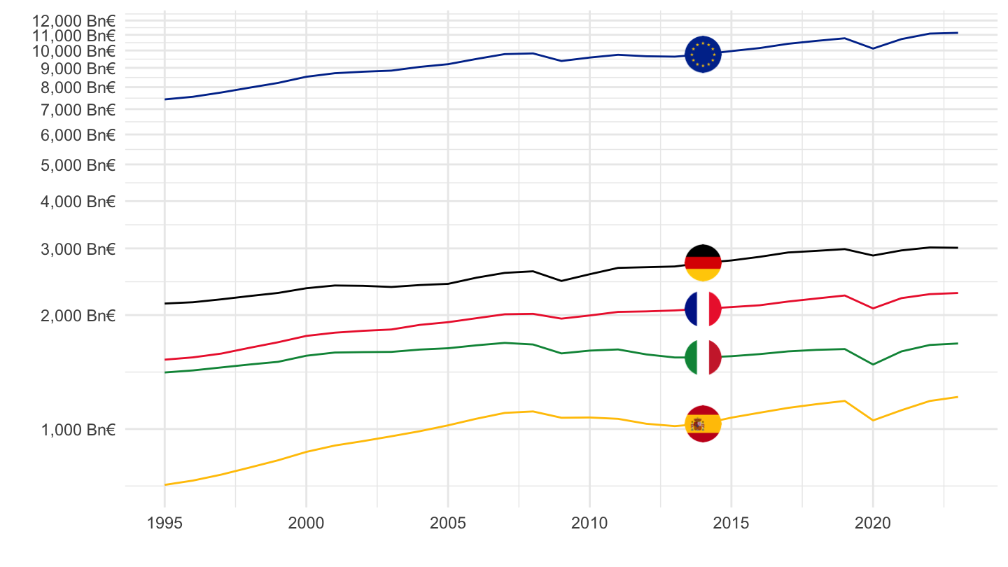
Index
Code
nama_10_gdp %>%
  filter(geo %in% c("FR", "DE", "EA20", "IT", "ES"),
         # B1GQ: Gross domestic product at market prices
         na_item == "B1GQ",
         unit == "CLV10_MEUR") %>%

  year_to_date %>%
  mutate(values = values/1000) %>%
  filter(date >= as.Date("1995-01-01")) %>%
  mutate(Geo = ifelse(geo == "EA20", "Europe", Geo)) %>%
  left_join(colors, by = c("Geo" = "country")) %>%
  group_by(Geo) %>%
  arrange(date) %>%
  mutate(values = 100*values/values[1]) %>%
  ggplot + geom_line(aes(x = date, y = values, color = color)) +
  scale_color_identity() + add_5flags + theme_minimal()  +
  scale_x_date(breaks = as.Date(paste0(seq(1960, 2100, 5), "-01-01")),
               labels = date_format("%Y")) +
  xlab("") + ylab("") +
  scale_y_log10(breaks = seq(100, 400, 5))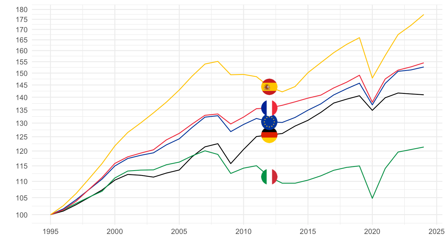
2010-
Index
Code
nama_10_gdp %>%
  filter(geo %in% c("FR", "DE", "EA20", "IT", "ES"),
         # B1GQ: Gross domestic product at market prices
         na_item == "B1GQ",
         unit == "CLV10_MEUR") %>%

  year_to_date %>%
  mutate(values = values/1000) %>%
  filter(date >= as.Date("2010-01-01")) %>%
  mutate(Geo = ifelse(geo == "EA20", "Europe", Geo)) %>%
  left_join(colors, by = c("Geo" = "country")) %>%
  group_by(Geo) %>%
  arrange(date) %>%
  mutate(values = 100*values/values[1]) %>%
  ggplot + geom_line(aes(x = date, y = values, color = color)) +
  scale_color_identity() + add_5flags + theme_minimal()  +
  scale_x_date(breaks = as.Date(paste0(seq(1960, 2100, 1), "-01-01")),
               labels = date_format("%Y")) +
  xlab("") + ylab("") +
  scale_y_log10(breaks = seq(100, 400, 5))
2010-2014
Index
Code
nama_10_gdp %>%
  filter(geo %in% c("FR", "DE", "EA20", "IT", "ES"),
         # B1GQ: Gross domestic product at market prices
         na_item == "B1GQ",
         unit == "CLV10_MEUR") %>%

  year_to_date %>%
  mutate(values = values/1000) %>%
  filter(date >= as.Date("2010-01-01"),
         date <= as.Date("2014-01-01")) %>%
  mutate(Geo = ifelse(geo == "EA20", "Europe", Geo)) %>%
  left_join(colors, by = c("Geo" = "country")) %>%
  group_by(Geo) %>%
  arrange(date) %>%
  mutate(values = 100*values/values[1]) %>%
  ggplot + geom_line(aes(x = date, y = values, color = color)) +
  scale_color_identity() + add_5flags + theme_minimal()  +
  scale_x_date(breaks = as.Date(paste0(seq(1960, 2100, 1), "-01-01")),
               labels = date_format("%Y")) +
  xlab("") + ylab("") +
  scale_y_log10(breaks = seq(10, 400, 1))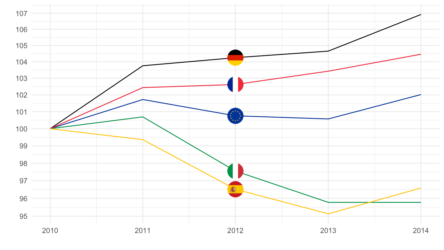
Germany, France, Italy, Spain, Netherlands, Belgium
Code
nama_10_gdp %>%
  filter(geo %in% c("FR", "DE", "IT", "ES", "NL", "BE"),
         # B1GQ: Gross domestic product at market prices
         na_item == "B1GQ",
         unit == "CLV10_MEUR") %>%

  year_to_date %>%
  mutate(values = values/1000) %>%
  filter(date >= as.Date("1995-01-01")) %>%
  mutate(Geo = ifelse(geo == "EA20", "Europe", Geo)) %>%
  left_join(colors, by = c("Geo" = "country")) %>%
  ggplot + geom_line(aes(x = date, y = values, color = color)) +
  scale_color_identity() + add_6flags + theme_minimal()  +
  scale_x_date(breaks = as.Date(paste0(seq(1960, 2100, 5), "-01-01")),
               labels = date_format("%Y")) +
  xlab("") + ylab("") +
  scale_y_log10(breaks = c(seq(100, 2100, 100), 1500, seq(1000, 15000, 1000)),
                labels = dollar_format(suffix = " Bn€", prefix = "", accuracy = 1))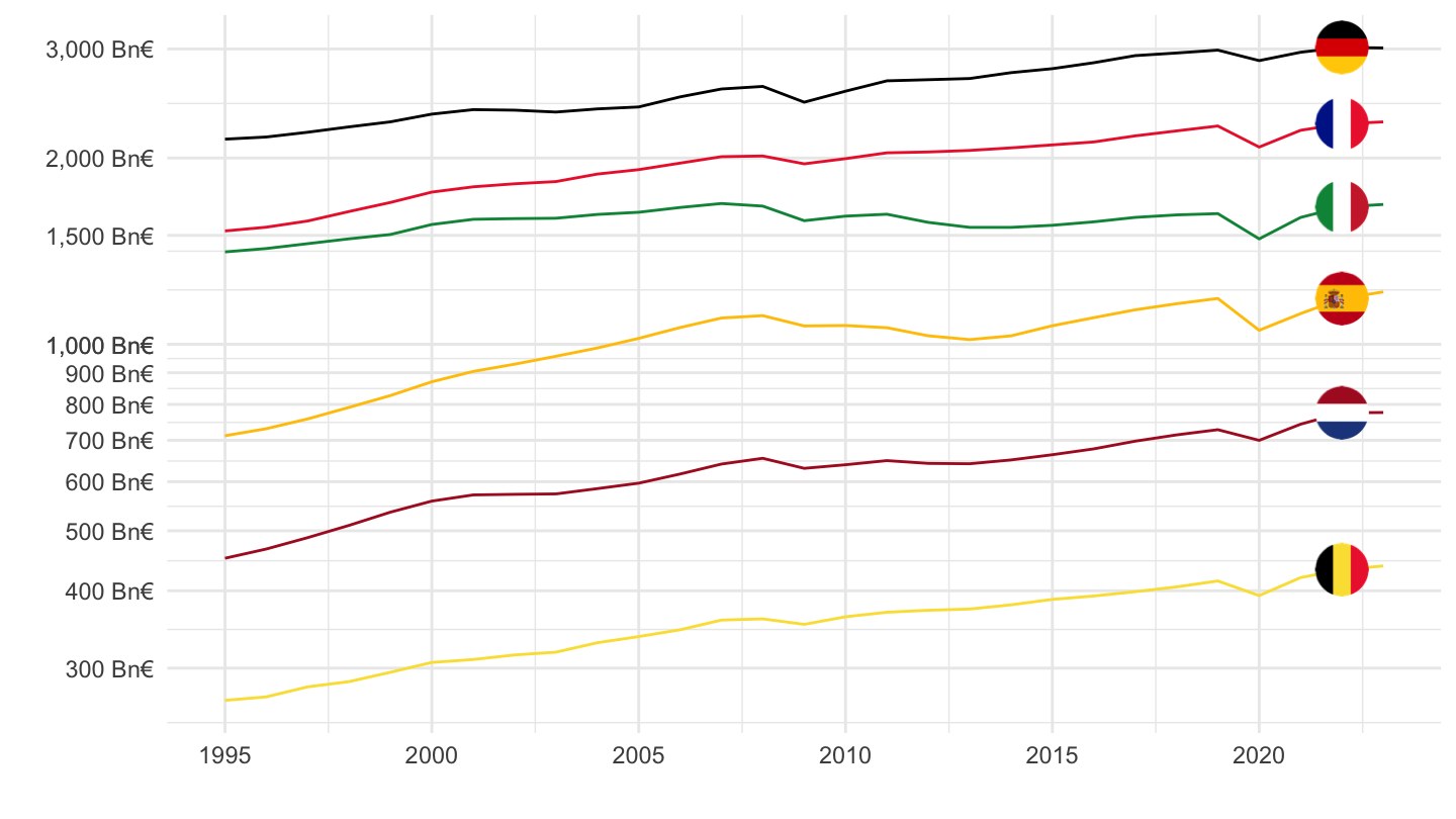
Investment Rates
France, Germany, Italy
Code
nama_10_gdp %>%
  filter(geo %in% c("FR", "DE", "IT"),
         na_item %in% c("B1GQ", "P51G"),
         unit == "CLV10_MEUR") %>%
  select(-unit) %>%
  spread(na_item, values) %>%
  mutate(values = P51G / B1GQ) %>%

  year_to_date %>%
  left_join(colors, by = c("Geo" = "country")) %>%
  ggplot + theme_minimal() + xlab("") + ylab("") +
  geom_line(aes(x = date, y = values, color = color)) +
  add_3flags + scale_color_identity() +
  scale_x_date(breaks = as.Date(paste0(seq(1960, 2100, 5), "-01-01")),
               labels = date_format("%Y")) +
  scale_y_continuous(breaks = 0.01*seq(0, 500, 1),
                labels = percent_format(accuracy = 1))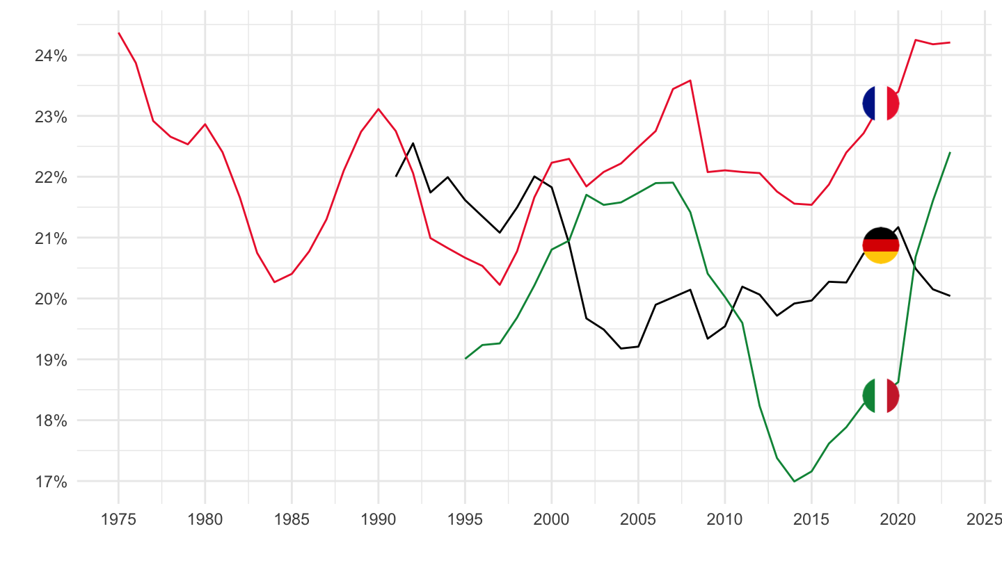
Deflator Index
France
Code
nama_10_gdp %>%
  filter(geo == "FR",
         time %in% c("2019", "1995"),
         unit == "PD15_EUR") %>%

  select_if(~ n_distinct(.) > 1) %>%
  spread(time, values) %>%
  mutate(`Change` = round(100*((`2019`/`1995`)^(1/24)-1),2)) %>%
  arrange(Change) %>%
print_table_conditional| na_item | Na_item | 1995 | 2019 | Change |
|---|---|---|---|---|
| D31 | Subsidies on products | 176.158 | 111.952 | -1.87 |
| P71 | Imports of goods | 94.770 | 101.683 | 0.29 |
| P61 | Exports of goods | 93.106 | 100.960 | 0.34 |
| P7 | Imports of goods and services | 91.610 | 102.167 | 0.46 |
| P6 | Exports of goods and services | 90.640 | 101.529 | 0.47 |
| P62 | Exports of services | 84.247 | 102.786 | 0.83 |
| P72 | Imports of services | 82.422 | 103.384 | 0.95 |
| P3_P6 | Final consumption expenditure, gross capital formation and exports of goods and services | 80.227 | 103.156 | 1.05 |
| P31_S14 | Final consumption expenditure of household | 80.411 | 103.728 | 1.07 |
| P31_S14_S15 | Household and NPISH final consumption expenditure | 80.202 | 103.750 | 1.08 |
| B1G | Value added, gross | 78.283 | 103.004 | 1.15 |
| P41 | Actual individual consumption | 78.465 | 103.437 | 1.16 |
| P3 | Final consumption expenditure | 77.903 | 103.418 | 1.19 |
| B1GQ | Gross domestic product at market prices | 77.394 | 103.471 | 1.22 |
| P3_P5 | Final consumption expenditure and gross capital formation | 77.519 | 103.680 | 1.22 |
| P5G | Gross capital formation | 76.310 | 104.597 | 1.32 |
| P51G | Gross fixed capital formation | 75.303 | 104.908 | 1.39 |
| P31_S15 | Final consumption expenditure of NPISH | 74.629 | 104.263 | 1.40 |
| P32_S13 | Collective consumption expenditure of general government | 73.677 | 103.265 | 1.42 |
| P3_S13 | Final consumption expenditure of general government | 72.723 | 102.668 | 1.45 |
| P31_S13 | Individual consumption expenditure of general government | 72.035 | 102.341 | 1.47 |
| D21 | Taxes on products | 74.556 | 107.356 | 1.53 |
| D21X31 | Taxes less subsidies on products | 70.168 | 107.162 | 1.78 |
P71 - Imports of goods
Code
nama_10_gdp %>%
  filter(na_item == "P71",
         unit == "PD15_EUR",
         geo %in% c("FR", "DE", "IT", "ES")) %>%
  year_to_date() %>%
  filter(date >= as.Date("1995-01-01")) %>%

  left_join(colors, by = c("Geo" = "country")) %>%
  group_by(Geo) %>%
  arrange(date) %>%
  mutate(values = values/ values[1]) %>%
  ggplot(.) + geom_line(aes(x = date, y = values, color = color)) +
  theme_minimal() + xlab("") + ylab("Price Deflator (P71)") +
  scale_color_identity() + add_4flags +
  scale_x_date(breaks = seq(1960, 2100, 5) %>% paste0("-01-01") %>% as.Date,
               labels = date_format("%Y")) +
  scale_y_continuous(breaks = 0.01*seq(-500, 200, 10))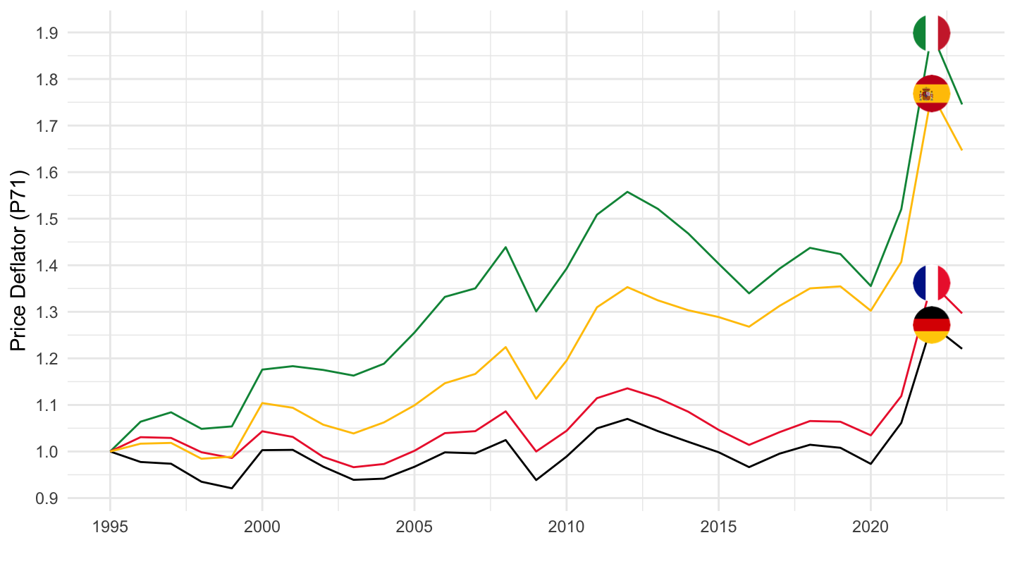
P61
Code
nama_10_gdp %>%
  filter(na_item == "P61",
         unit == "PD15_EUR",
         geo %in% c("FR", "DE", "IT", "ES")) %>%
  year_to_date() %>%
  filter(date >= as.Date("1995-01-01")) %>%

  left_join(colors, by = c("Geo" = "country")) %>%
  group_by(Geo) %>%
  arrange(date) %>%
  mutate(values = values/ values[1]) %>%
  ggplot(.) + geom_line(aes(x = date, y = values, color = color)) +
  theme_minimal() + xlab("") + ylab("Price Deflator (P61)") +
  scale_color_identity() + add_4flags +
  scale_x_date(breaks = seq(1960, 2100, 5) %>% paste0("-01-01") %>% as.Date,
               labels = date_format("%Y")) +
  scale_y_continuous(breaks = 0.01*seq(-500, 200, 10))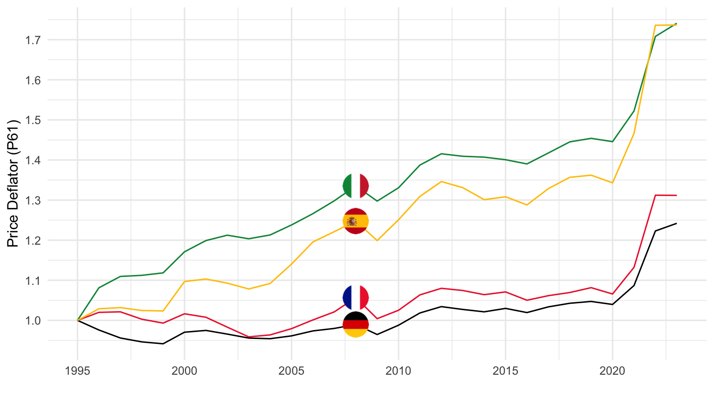
P5G
Code
nama_10_gdp %>%
  filter(na_item == "P5G",
         unit == "PD15_EUR",
         geo %in% c("FR", "DE", "IT", "ES")) %>%
  year_to_date() %>%
  filter(date >= as.Date("1995-01-01")) %>%

  left_join(colors, by = c("Geo" = "country")) %>%
  group_by(Geo) %>%
  arrange(date) %>%
  mutate(values = values/ values[1]) %>%
  ggplot(.) + geom_line(aes(x = date, y = values, color = color)) +
  theme_minimal() + xlab("") + ylab("Price Deflator (P5G)") +
  scale_color_identity() + add_4flags +
  scale_x_date(breaks = seq(1960, 2100, 5) %>% paste0("-01-01") %>% as.Date,
               labels = date_format("%Y")) +
  scale_y_continuous(breaks = 0.01*seq(-500, 200, 10))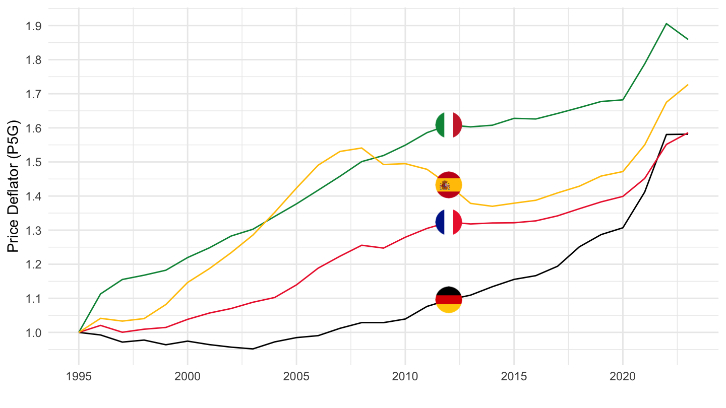
P3
Code
nama_10_gdp %>%
  filter(na_item == "P3",
         unit == "PD15_EUR",
         geo %in% c("FR", "DE", "IT", "ES")) %>%
  year_to_date() %>%
  filter(date >= as.Date("1995-01-01")) %>%

  left_join(colors, by = c("Geo" = "country")) %>%
  group_by(Geo) %>%
  arrange(date) %>%
  mutate(values = values/ values[1]) %>%
  ggplot(.) + geom_line(aes(x = date, y = values, color = color)) +
  theme_minimal() + xlab("") + ylab("Price Deflator (P31_S14)") +
  scale_color_identity() + add_4flags +
  scale_x_date(breaks = seq(1960, 2100, 5) %>% paste0("-01-01") %>% as.Date,
               labels = date_format("%Y")) +
  scale_y_continuous(breaks = 0.01*seq(-500, 200, 10))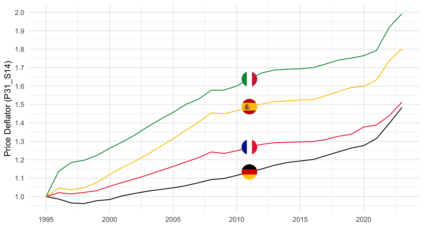
P31_S14 - Final consumption expenditure of households
Code
nama_10_gdp %>%
  filter(na_item == "P31_S14",
         unit == "PD15_EUR",
         geo %in% c("FR", "DE", "IT", "ES")) %>%
  year_to_date() %>%
  filter(date >= as.Date("1995-01-01")) %>%

  left_join(colors, by = c("Geo" = "country")) %>%
  group_by(Geo) %>%
  arrange(date) %>%
  mutate(values = values/ values[1]) %>%
  ggplot(.) + geom_line(aes(x = date, y = values, color = color)) +
  theme_minimal() + xlab("") + ylab("Price Deflator (P31_S14)") +
  scale_color_identity() + add_4flags +
  scale_x_date(breaks = seq(1960, 2100, 5) %>% paste0("-01-01") %>% as.Date,
               labels = date_format("%Y")) +
  scale_y_continuous(breaks = 0.01*seq(-500, 200, 10))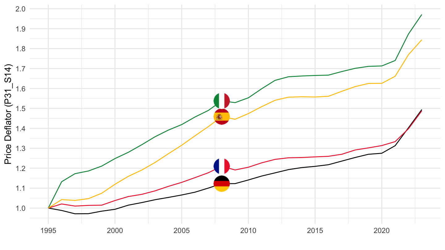
P31_S15
Code
nama_10_gdp %>%
  filter(na_item == "P31_S15",
         unit == "PD15_EUR",
         geo %in% c("FR", "DE", "IT", "ES")) %>%
  year_to_date() %>%
  filter(date >= as.Date("1995-01-01")) %>%

  left_join(colors, by = c("Geo" = "country")) %>%
  group_by(Geo) %>%
  arrange(date) %>%
  mutate(values = values/ values[1]) %>%
  ggplot(.) + geom_line(aes(x = date, y = values, color = color)) +
  theme_minimal() + xlab("") + ylab("Price Deflator (P31_S15)") +
  scale_color_identity() + add_4flags +
  scale_x_date(breaks = seq(1960, 2100, 5) %>% paste0("-01-01") %>% as.Date,
               labels = date_format("%Y")) +
  scale_y_continuous(breaks = 0.01*seq(-500, 200, 10))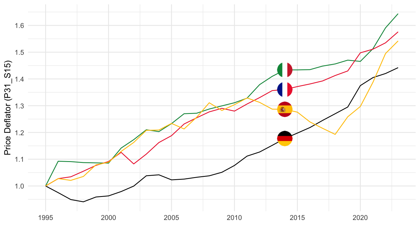
P31_S14_S15
Code
nama_10_gdp %>%
  filter(na_item == "P31_S14_S15",
         unit == "PD15_EUR",
         geo %in% c("FR", "DE", "IT", "ES")) %>%
  year_to_date() %>%
  filter(date >= as.Date("1995-01-01")) %>%

  left_join(colors, by = c("Geo" = "country")) %>%
  group_by(Geo) %>%
  arrange(date) %>%
  mutate(values = values/ values[1]) %>%
  ggplot(.) + geom_line(aes(x = date, y = values, color = color)) +
  theme_minimal() + xlab("") + ylab("Price Deflator (P31_S14_S15)") +
  scale_color_identity() + add_4flags +
  scale_x_date(breaks = seq(1960, 2100, 5) %>% paste0("-01-01") %>% as.Date,
               labels = date_format("%Y")) +
  scale_y_continuous(breaks = 0.01*seq(-500, 200, 10))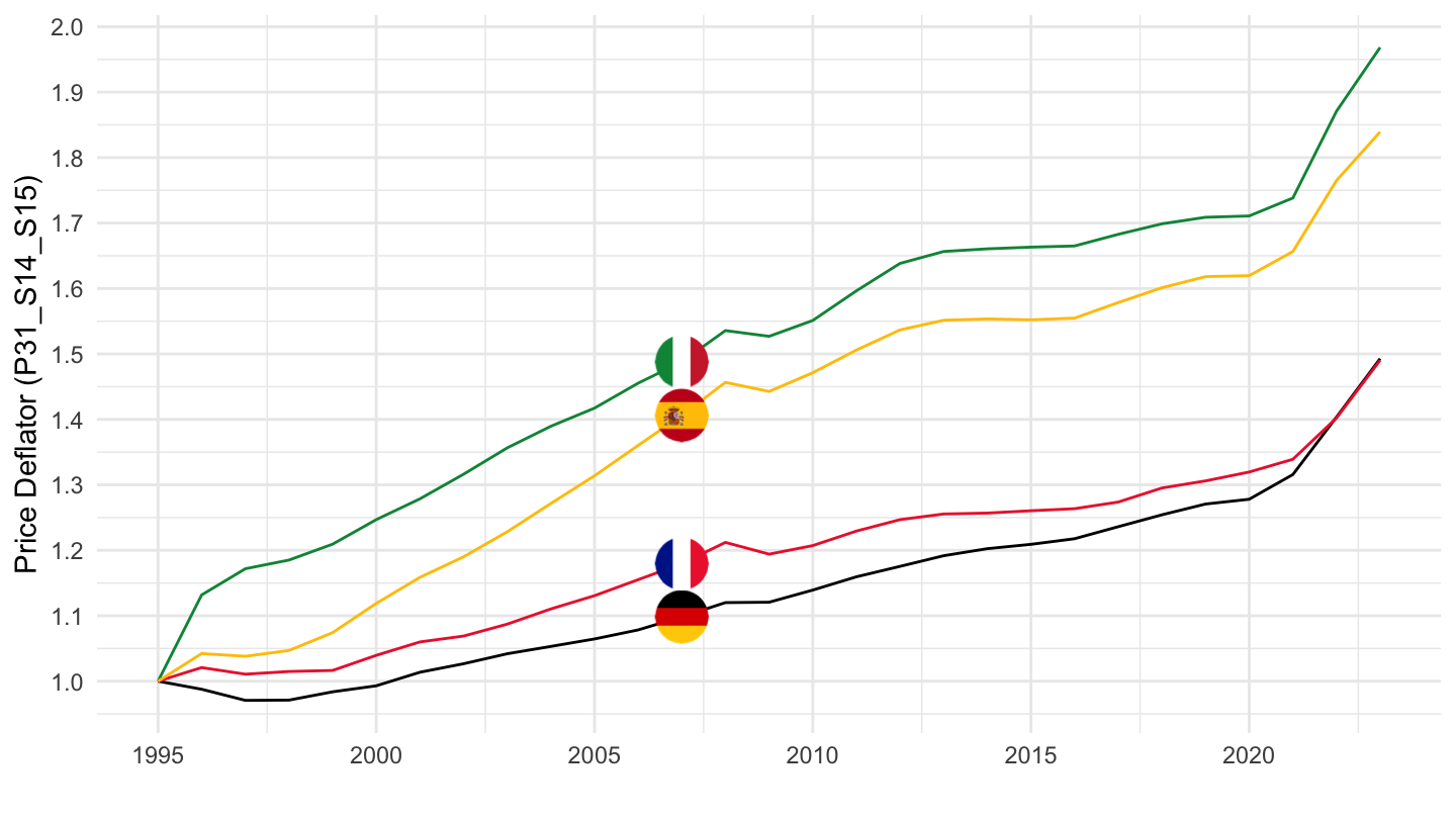
B1G
Code
nama_10_gdp %>%
  filter(na_item == "B1G",
         unit == "PD15_EUR",
         geo %in% c("FR", "DE", "IT", "ES")) %>%
  year_to_date() %>%
  filter(date >= as.Date("1995-01-01")) %>%

  left_join(colors, by = c("Geo" = "country")) %>%
  group_by(Geo) %>%
  arrange(date) %>%
  mutate(values = values/ values[1]) %>%
  ggplot(.) + geom_line(aes(x = date, y = values, color = color)) +
  theme_minimal() + xlab("") + ylab("Price Deflator (B1G)") +
  scale_color_identity() + add_4flags +
  scale_x_date(breaks = seq(1960, 2100, 5) %>% paste0("-01-01") %>% as.Date,
               labels = date_format("%Y")) +
  scale_y_continuous(breaks = 0.01*seq(-500, 200, 10))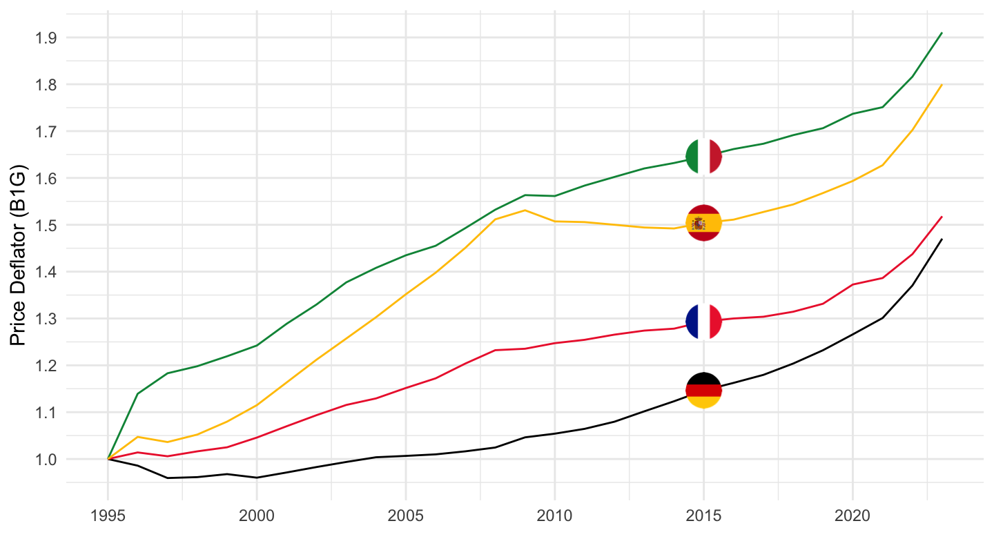
B1GQ
Code
nama_10_gdp %>%
  filter(na_item == "B1GQ",
         unit == "PD15_EUR",
         geo %in% c("FR", "DE", "IT", "ES")) %>%
  year_to_date() %>%
  filter(date >= as.Date("1995-01-01")) %>%

  left_join(colors, by = c("Geo" = "country")) %>%
  group_by(Geo) %>%
  arrange(date) %>%
  mutate(values = values/ values[1]) %>%
  ggplot(.) + geom_line(aes(x = date, y = values, color = color)) +
  theme_minimal() + xlab("") + ylab("Price Deflator (B1GQ)") +
  scale_color_identity() + add_4flags +
  scale_x_date(breaks = seq(1960, 2100, 5) %>% paste0("-01-01") %>% as.Date,
               labels = date_format("%Y")) +
  scale_y_continuous(breaks = 0.01*seq(-500, 200, 10))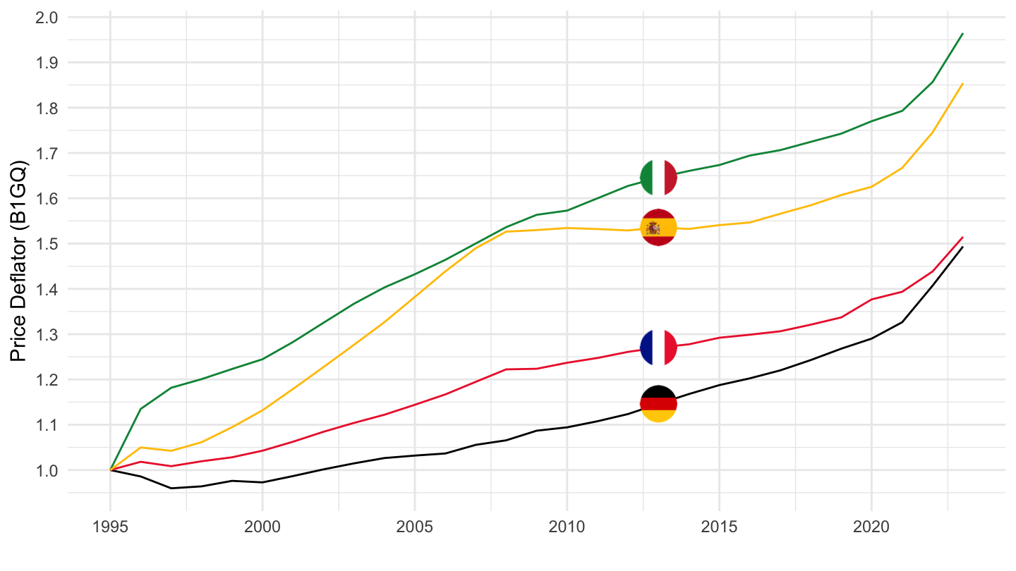
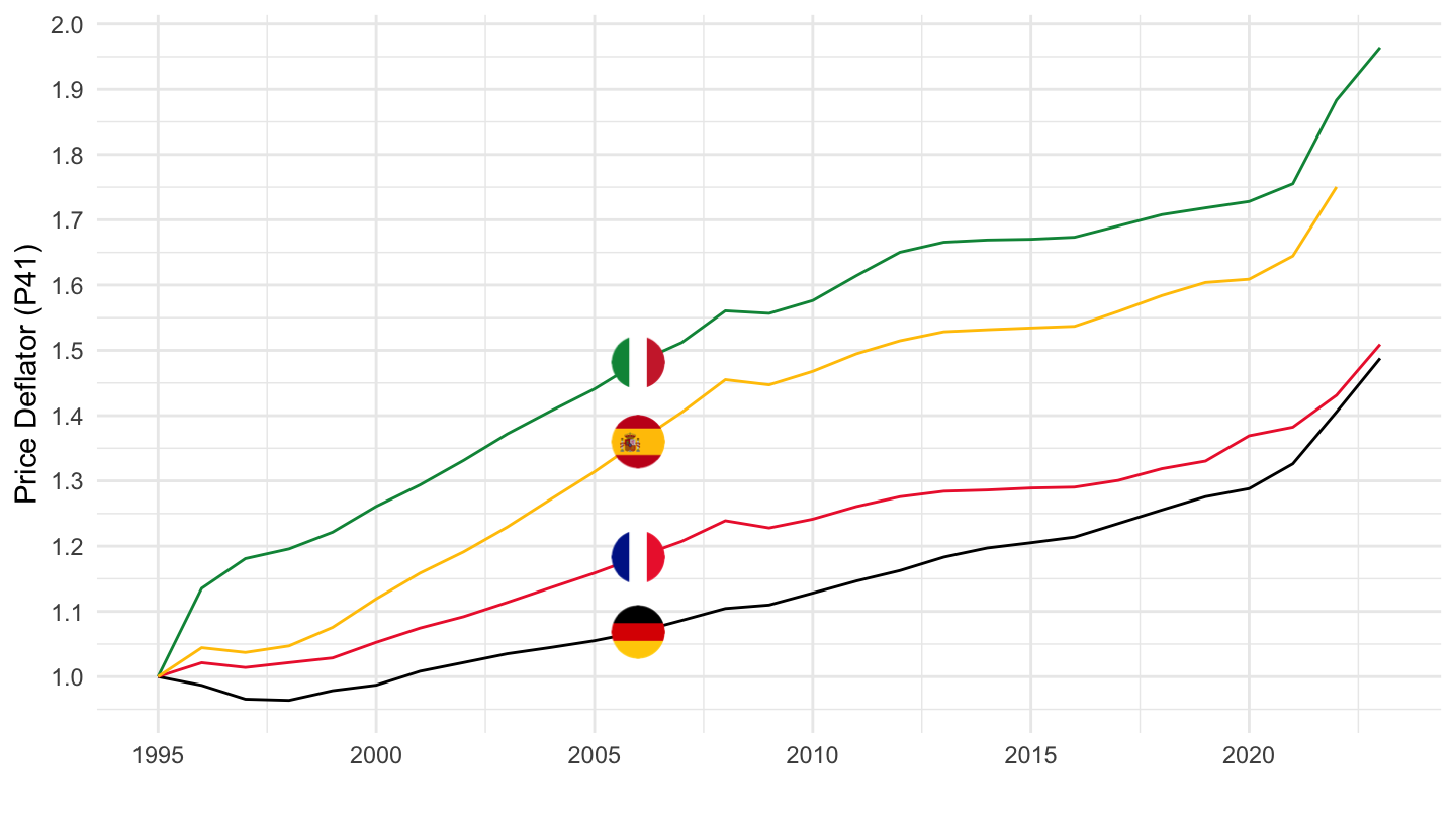
P41
Code
nama_10_gdp %>%
  filter(na_item == "P41",
         unit == "PD15_EUR",
         geo %in% c("FR", "DE", "IT", "ES")) %>%
  year_to_date() %>%
  filter(date >= as.Date("1995-01-01")) %>%

  left_join(colors, by = c("Geo" = "country")) %>%
  group_by(Geo) %>%
  arrange(date) %>%
  mutate(values = values/ values[1]) %>%
  ggplot(.) + geom_line(aes(x = date, y = values, color = color)) +
  theme_minimal() + xlab("") + ylab("Price Deflator (P41)") +
  scale_color_identity() + add_4flags +
  scale_x_date(breaks = seq(1960, 2100, 5) %>% paste0("-01-01") %>% as.Date,
               labels = date_format("%Y")) +
  scale_y_continuous(breaks = 0.01*seq(-500, 200, 10))