| source | dataset | .html | .RData |
|---|---|---|---|
| 2024-09-11 | 2024-04-30 |
PPPs and exchange rates
Data - OECD
Info
Data on xrates
| source | dataset | .html | .RData |
|---|---|---|---|
| 2024-07-26 | 2024-06-18 | ||
| 2024-08-09 | 2024-08-28 | ||
| 2024-08-28 | 2024-05-10 | ||
| 2024-05-10 | 2024-09-14 | ||
| 2024-08-28 | 2024-08-28 | ||
| 2024-09-14 | 2024-09-14 | ||
| 2024-09-14 | 2024-08-28 | ||
| 2024-09-14 | 2024-06-08 | ||
| 2024-09-14 | 2024-09-14 | ||
| 2024-06-20 | 2021-01-08 | ||
| 2024-09-15 | 2024-04-30 | ||
| 2024-09-11 | 2024-04-30 | ||
| 2024-08-28 | 2024-09-15 |
Data on industry
| source | dataset | .html | .RData |
|---|---|---|---|
| 2024-09-15 | 2023-10-01 | ||
| 2024-09-14 | 2024-09-14 | ||
| 2024-09-14 | 2024-09-14 | ||
| 2024-09-14 | 2024-09-14 | ||
| 2024-09-14 | 2024-09-14 | ||
| 2024-09-14 | 2024-09-14 | ||
| 2024-09-14 | 2024-09-14 | ||
| 2024-06-24 | 2024-09-14 | ||
| 2024-09-15 | 2024-09-14 | ||
| 2024-09-15 | 2024-09-14 | ||
| 2024-06-24 | 2024-09-14 | ||
| 2024-09-14 | 2024-09-14 | ||
| 2024-04-16 | 2024-05-12 | ||
| 2024-04-16 | 2023-09-09 | ||
| 2024-04-16 | 2023-11-22 | ||
| 2024-05-12 | 2024-05-03 | ||
| 2024-09-15 | 2023-10-04 | ||
| 2024-09-11 | 2024-04-30 | ||
| 2024-01-06 | 2024-09-15 | ||
| 2024-09-15 | 2024-09-15 | ||
| 2024-01-06 | 2024-09-15 | ||
| 2024-01-06 | 2024-09-15 | ||
| 2024-01-06 | 2024-09-15 | ||
| 2024-01-06 | 2024-09-15 | ||
| 2024-01-06 | 2024-09-15 |
COMPILE_TIME
| COMPILE_TIME |
|---|
| 2024-09-15 |
Last
| obsTime | Nobs |
|---|---|
| 2023 | 110 |
TRANSACT
Code
SNA_TABLE4 %>%
  left_join(SNA_TABLE4_var$TRANSACT, by = "TRANSACT") %>%
  group_by(TRANSACT, Transact) %>%
  summarise(Nobs = n()) %>%
  arrange(-Nobs) %>%
{if (is_html_output()) print_table(.) else .}| TRANSACT | Transact | Nobs |
|---|---|---|
| EXC | Exchange rates, period-average | 4159 |
| EXCE | Exchange rates, end of period | 3451 |
| PPPGDP | Purchasing Power Parities for GDP | 2994 |
| PPPPRC | Purchasing Power Parities for private consumption | 2599 |
| PPPP41 | Purchasing Power Parities for actual individual consumption | 2051 |
MEASURE
Code
SNA_TABLE4 %>%
  left_join(SNA_TABLE4_var$MEASURE, by = "MEASURE") %>%
  group_by(MEASURE, Measure) %>%
  summarise(Nobs = n()) %>%
  arrange(-Nobs) %>%
{if (is_html_output()) print_table(.) else .}| MEASURE | Measure | Nobs |
|---|---|---|
| CD | National currency per US dollar | 15254 |
LOCATION
Code
SNA_TABLE4 %>%
  left_join(SNA_TABLE4_var$LOCATION, by = "LOCATION") %>%
  group_by(LOCATION, Location) %>%
  summarise(Nobs = n()) %>%
  arrange(-Nobs) %>%
  {if (is_html_output()) datatable(., filter = 'top', rownames = F) else .}
Exchange Rate
Flat
Code
include_graphics3b("bib/oecd/SNA_TABLE4_ex1.png")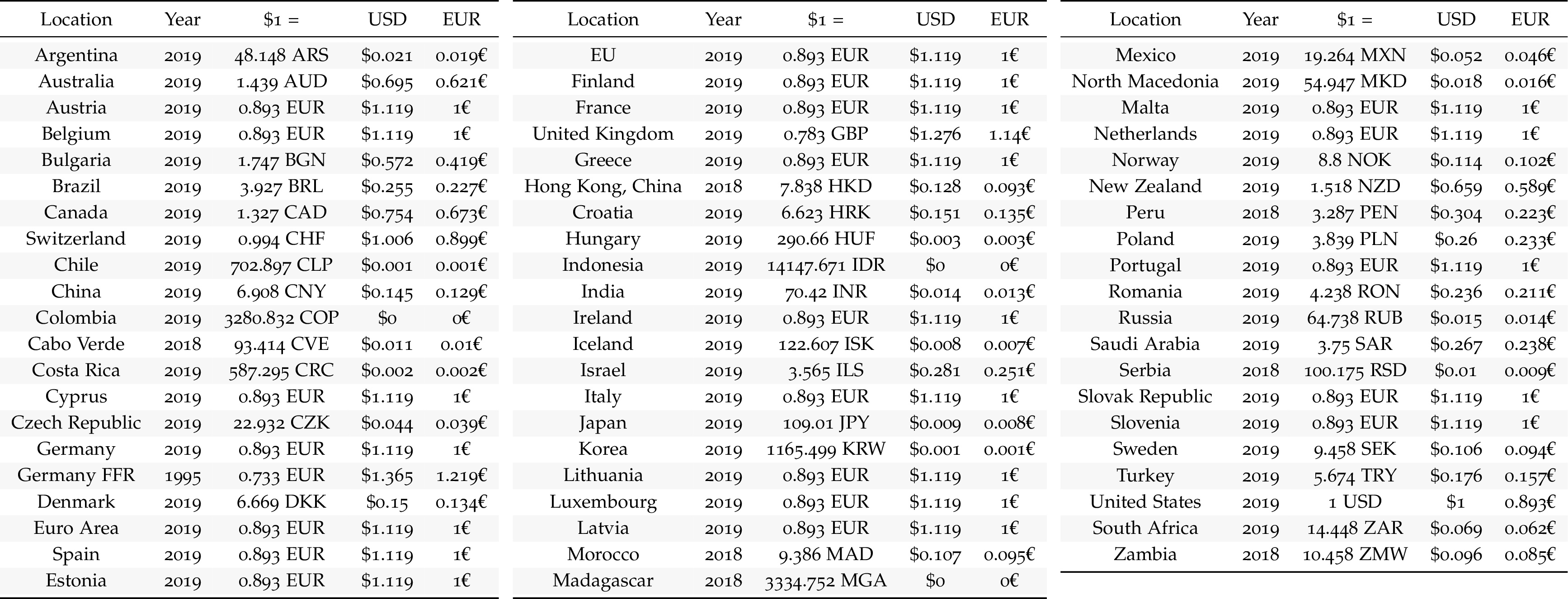
Javascript
Code
SNA_TABLE4 %>%
  filter(TRANSACT == "EXC") %>%
  left_join(SNA_TABLE4_var$LOCATION, by = "LOCATION") %>%
  group_by(LOCATION, UNIT, Location) %>%
  summarise(year_first = first(obsTime),
            year_last = last(obsTime),
            `$1 = ` = last(obsValue)) %>%
  ungroup %>%
  mutate(`USD` = paste0("$", round(1/`$1 = `, 3)),
         `EUR` = paste0(round(`$1 = `[UNIT == "EUR"]/`$1 = `, 3), "€"),
         `$1 = ` = paste0(round(`$1 = `, 3), " ", UNIT)) %>%
  select(-UNIT) %>%
  mutate(Loc = gsub(" ", "-", str_to_lower(Location)),
         Loc = paste0('<img src="../../bib/flags/vsmall/', Loc, '.png" alt="Flag">')) %>%
  select(Loc, everything()) %>%
  {if (is_html_output()) datatable(., filter = 'top', rownames = F, escape = F) else .}
EXC - Period Average: Time Series
Argentina
Code
SNA_TABLE4 %>%
  filter(TRANSACT == "EXC",
         LOCATION == "ARG") %>%
  year_to_date() %>%
  ggplot(.) + theme_minimal() +
  geom_line(aes(x = date, y = obsValue)) +
  xlab("") + ylab("$1 in Argentine Pesos") +
  scale_x_date(breaks = seq(1940, 2020, 5) %>% paste0("-01-01") %>% as.Date,
               labels = date_format("%Y")) +
  scale_y_log10(breaks = 10^seq(-6, 2, 1),
                labels = dollar_format(a = 0.000001, p = "$ ", su = "/$"))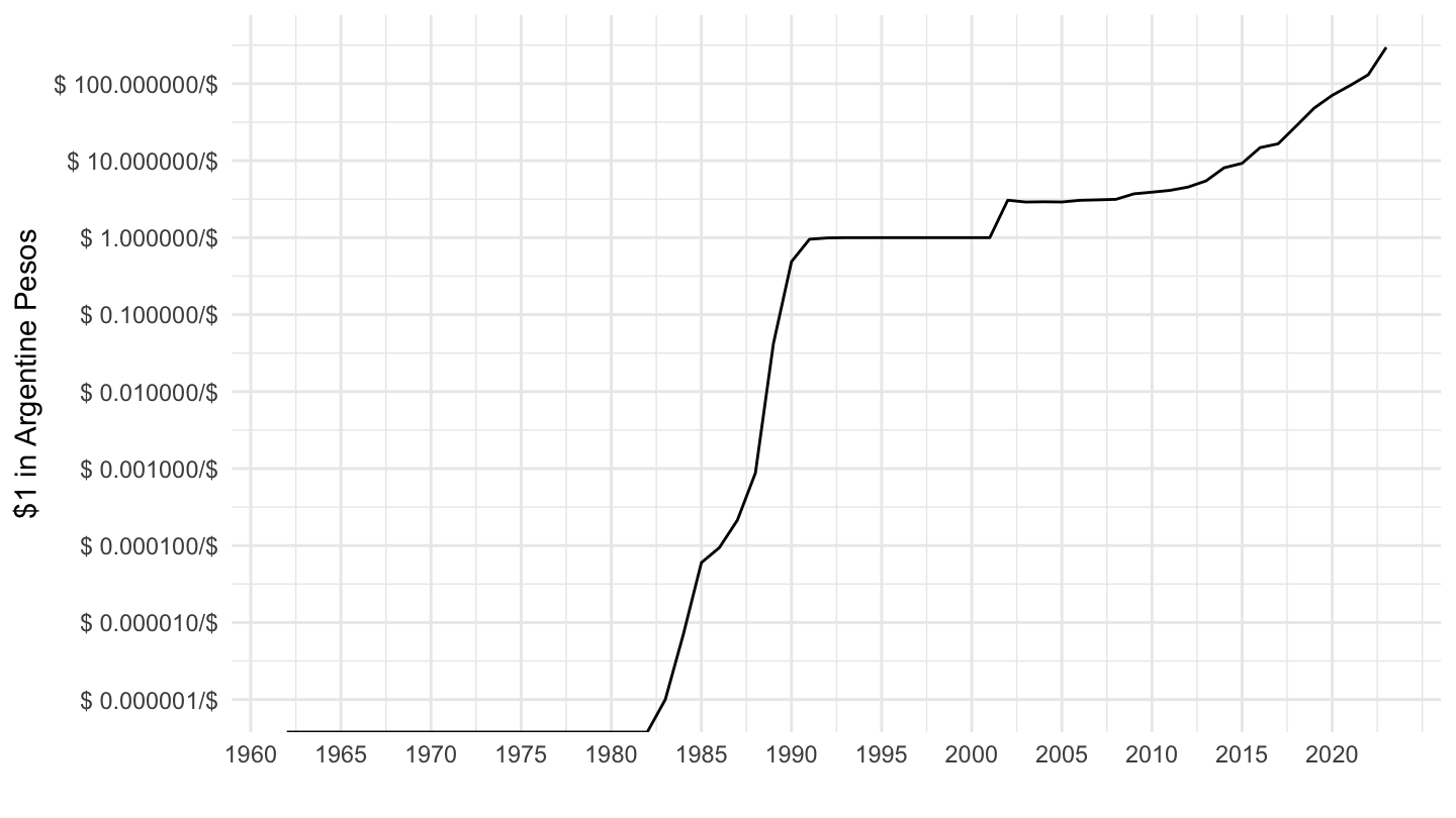
Australia, Austria, Belgium
Code
SNA_TABLE4 %>%
  filter(TRANSACT == "EXC",
         LOCATION %in% c("AUS", "AUT", "BEL")) %>%
  left_join(SNA_TABLE4_var$LOCATION, by = "LOCATION") %>%
  left_join(colors, by = c("Location" = "country")) %>%
  year_to_date() %>%
  ggplot(.) + theme_minimal() + scale_color_identity() +
  geom_line(aes(x = date, y = obsValue, color = color)) +
  add_3flags + xlab("") + ylab("Exchange Rate ($1 = ? National Currency)") +
  scale_x_date(breaks = seq(1940, 2020, 5) %>% paste0("-01-01") %>% as.Date,
               labels = date_format("%Y")) +
  scale_y_log10(breaks = seq(0, 10, 0.1),
                     labels = dollar_format(a = 0.1, p = "", su = " ../$"))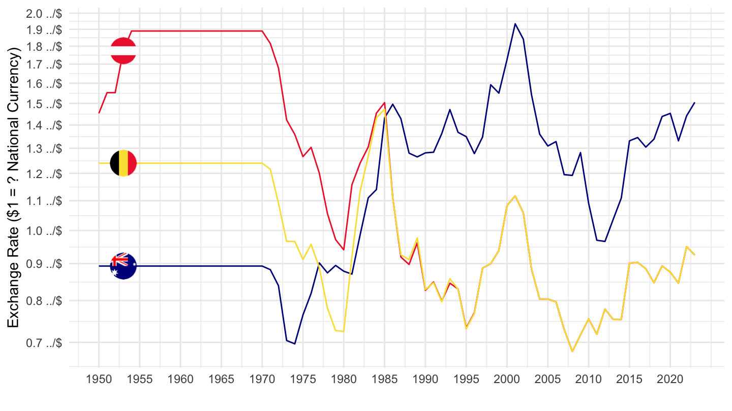
Bulgaria
Code
SNA_TABLE4 %>%
  filter(TRANSACT == "EXC",
         LOCATION == "BGR") %>%
  year_to_date() %>%
  ggplot(.) + theme_minimal() +
  geom_line(aes(x = date, y = obsValue)) +
  xlab("") + ylab("$1 in Bulgarian lev") +
  scale_x_date(breaks = seq(1940, 2020, 5) %>% paste0("-01-01") %>% as.Date,
               labels = date_format("%Y")) +
  scale_y_log10(breaks = c(c(0, 0.1, 0.2, 0.3, 0.5, 1, 2, 3),
                           0.1*c(0, 0.1, 0.2, 0.3, 0.5, 1),
                           0.01*c(0, 0.1, 0.2, 0.3, 0.5, 1)),
                     labels = dollar_format(a = 0.001, p = "", su = " lev/$"))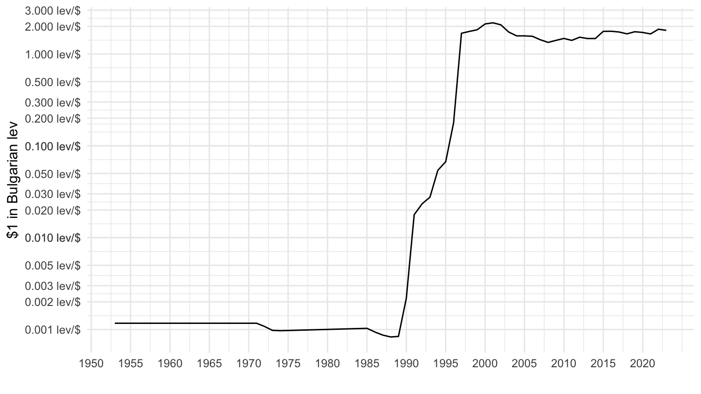
Brazil
Code
SNA_TABLE4 %>%
  filter(TRANSACT == "EXC",
         LOCATION == "BRA") %>%
  year_to_date() %>%
  ggplot(.) + theme_minimal() +
  geom_line(aes(x = date, y = obsValue)) +
  xlab("") + ylab("$1 in Brazilian Real") +
  scale_x_date(breaks = seq(1940, 2020, 5) %>% paste0("-01-01") %>% as.Date,
               labels = date_format("%Y")) +
  scale_y_log10(breaks = 10^seq(-6, 2, 1),
                labels = dollar_format(a = 0.000001, p = "", su = " R$/$"))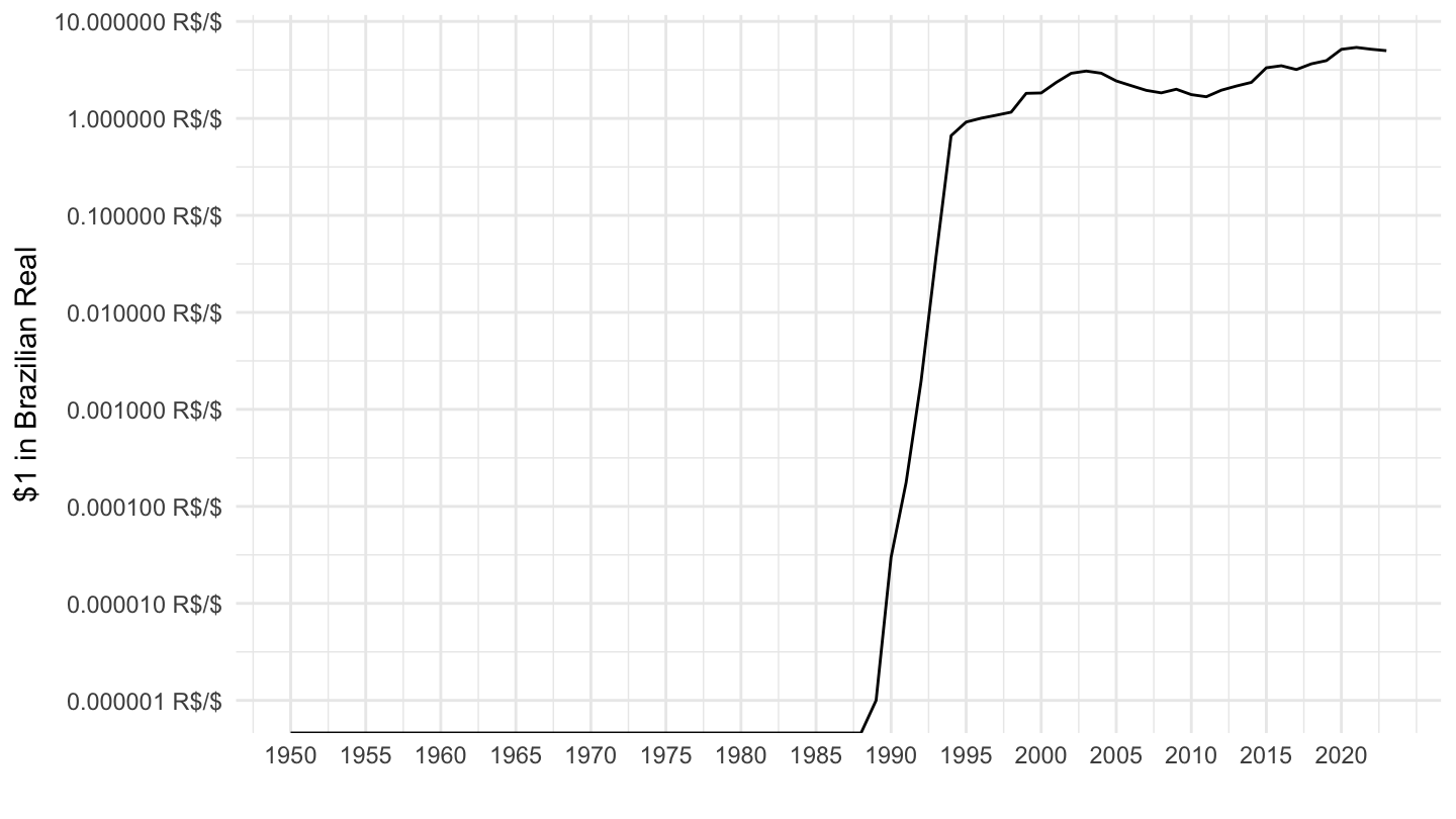
France, Germany, Italy, Spain, Greece
Code
SNA_TABLE4 %>%
  filter(TRANSACT == "EXC",
         LOCATION %in% c("FRA", "DEU", "ITA", "ESP", "GRC")) %>%
  left_join(SNA_TABLE4_var$LOCATION, by = "LOCATION") %>%
  left_join(colors, by = c("Location" = "country")) %>%
  year_to_date() %>%
  ggplot(.) + theme_minimal() + scale_color_identity() +
  geom_line(aes(x = date, y = obsValue, color = color)) +
  add_5flags + xlab("") + ylab("Exchange Rate ($1 = ? National Currency)") +
  scale_x_date(breaks = seq(1940, 2020, 5) %>% paste0("-01-01") %>% as.Date,
               labels = date_format("%Y")) +
  scale_y_log10(breaks = seq(0, 10, 0.1),
                     labels = dollar_format(a = 0.1, p = "", su = " ../$"))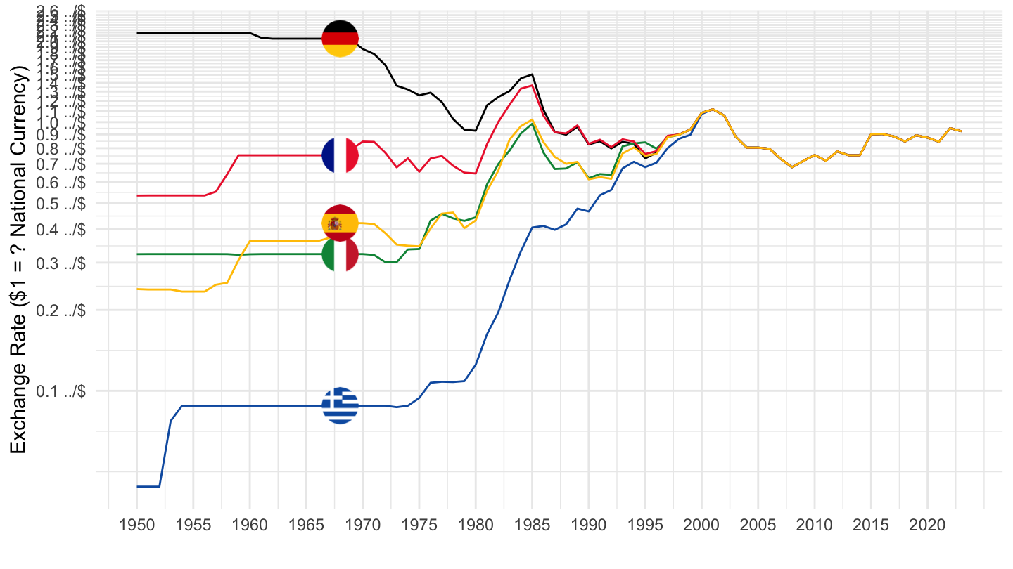
Canada, United Kingdom
Code
SNA_TABLE4 %>%
  filter(TRANSACT == "EXC",
         LOCATION %in% c("CAN", "GBR", "DEU")) %>%
  left_join(SNA_TABLE4_var$LOCATION, by = "LOCATION") %>%
  left_join(colors, by = c("Location" = "country")) %>%
  year_to_date() %>%
  ggplot(.) + theme_minimal() + scale_color_identity() +
  geom_line(aes(x = date, y = obsValue, color = color)) +
  add_3flags + xlab("") + ylab("Exchange Rate ($1 = ? National Currency)") +
  scale_x_date(breaks = seq(1940, 2020, 5) %>% paste0("-01-01") %>% as.Date,
               labels = date_format("%Y")) +
  scale_y_log10(breaks = seq(0, 10, 0.1),
                     labels = dollar_format(a = 0.1, p = "", su = " ../$"))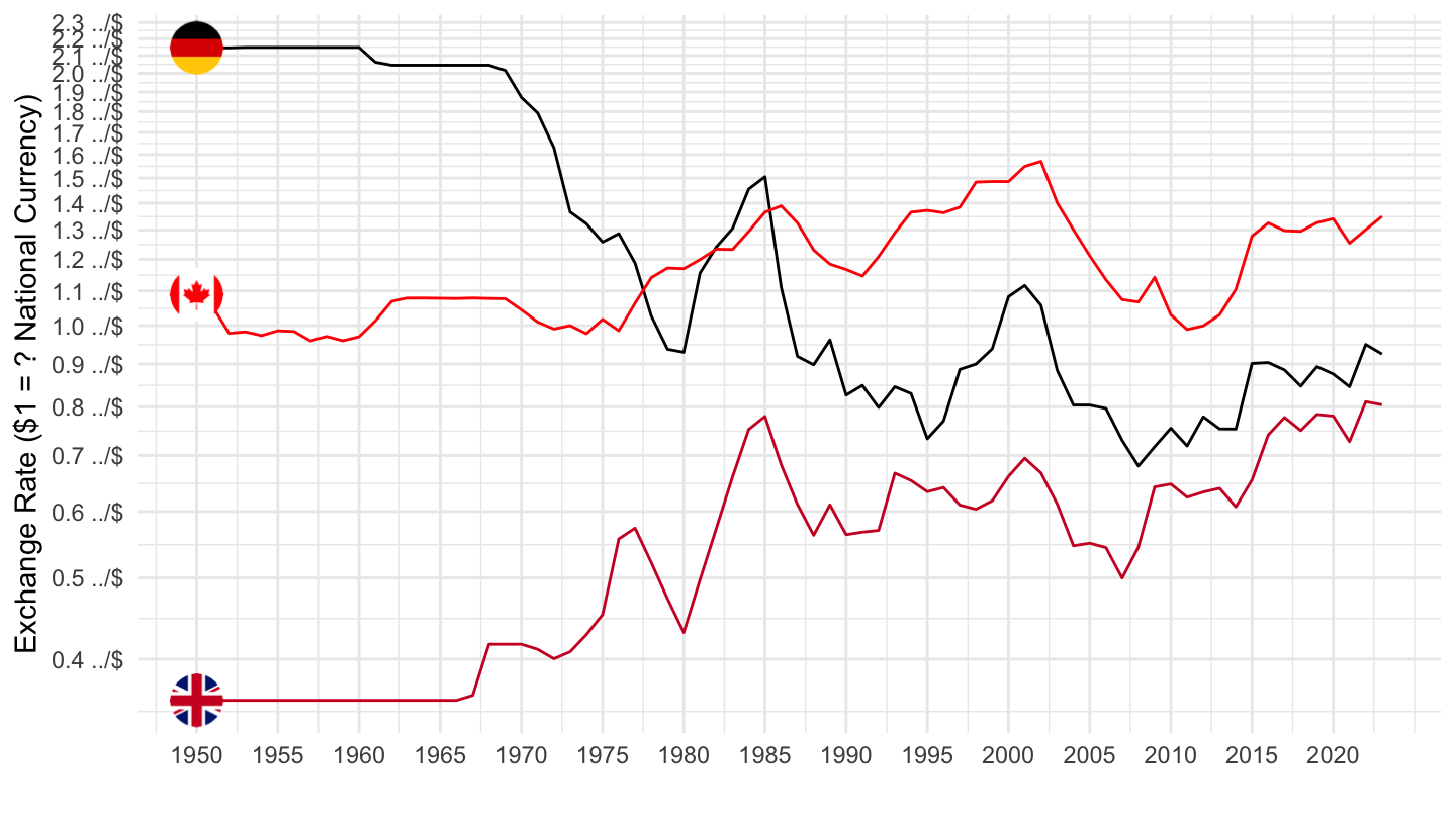
Switzerland, United Kingdom
Code
SNA_TABLE4 %>%
  filter(TRANSACT == "EXC",
         LOCATION %in% c("CHE", "GBR", "DEU")) %>%
  left_join(SNA_TABLE4_var$LOCATION, by = "LOCATION") %>%
  left_join(colors, by = c("Location" = "country")) %>%
  year_to_date() %>%
  ggplot(.) + theme_minimal() + scale_color_identity() +
  geom_line(aes(x = date, y = obsValue, color = color)) +
  add_3flags + xlab("") + ylab("Exchange Rate ($1 = ? National Currency)") +
  scale_x_date(breaks = seq(1940, 2020, 5) %>% paste0("-01-01") %>% as.Date,
               labels = date_format("%Y")) +
  scale_y_log10(breaks = seq(0, 10, 0.1),
                     labels = dollar_format(a = 0.1, p = "", su = " ../$"))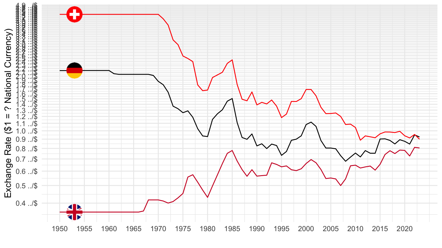
Chile
Code
SNA_TABLE4 %>%
  filter(TRANSACT == "EXC",
         LOCATION == "CHL") %>%
  year_to_date() %>%
  ggplot(.) + theme_minimal() +
  geom_line(aes(x = date, y = obsValue)) +
  xlab("") + ylab("$1 in Chilean Peso") +
  scale_x_date(breaks = seq(1940, 2020, 5) %>% paste0("-01-01") %>% as.Date,
               labels = date_format("%Y")) +
  scale_y_log10(breaks = 10^seq(-6, 3, 1),
                labels = dollar_format(a = 0.0001, p = "", su = " CLP/$"))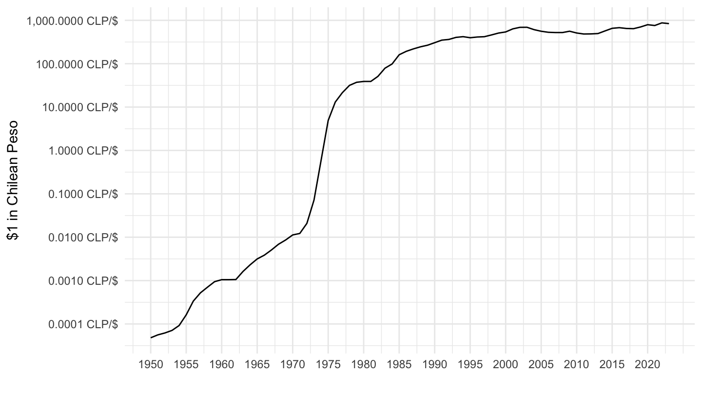
China
Code
SNA_TABLE4 %>%
  filter(TRANSACT == "EXC",
         LOCATION == "CHN") %>%
  year_to_date() %>%
  ggplot(.) + theme_minimal() +
  geom_line(aes(x = date, y = obsValue)) +
  xlab("") + ylab("$1 in Chinese Yuan") +
  scale_x_date(breaks = seq(1940, 2020, 5) %>% paste0("-01-01") %>% as.Date,
               labels = date_format("%Y")) +
  scale_y_log10(breaks = seq(1, 10, 1),
                     labels = dollar_format(a = 1, p = "", su = " ¥/$"))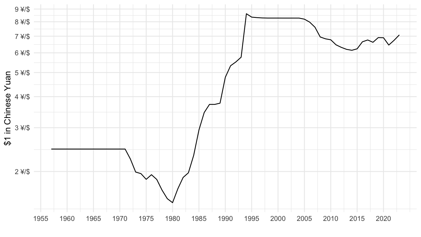
Colombia
Code
SNA_TABLE4 %>%
  filter(TRANSACT == "EXC",
         LOCATION == "COL") %>%
  year_to_date() %>%
  ggplot(.) + theme_minimal() +
  geom_line(aes(x = date, y = obsValue)) +
  xlab("") + ylab("$1 in Colombian Peso") +
  scale_x_date(breaks = seq(1940, 2020, 5) %>% paste0("-01-01") %>% as.Date,
               labels = date_format("%Y")) +
  scale_y_log10(breaks = c(5, 10, 20, 30, 50,
                           100, 200, 300, 500,
                           1000, 2000, 3000, 5000),
                labels = dollar_format(a = 1, p = "", su = " COL$/$"))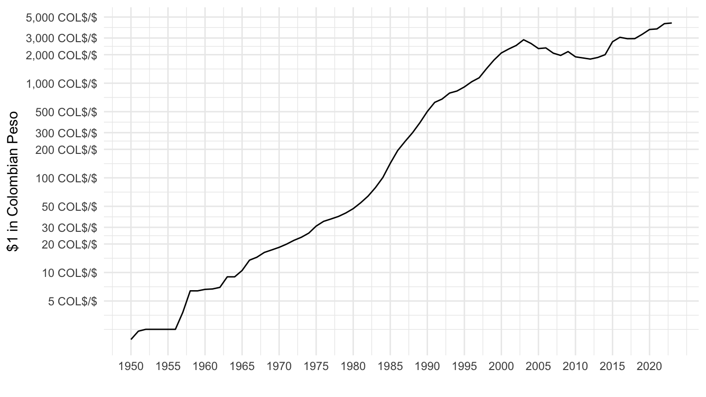
EXCE - End of Period: Time Series
Argentina
Code
SNA_TABLE4 %>%
  filter(TRANSACT == "EXCE",
         LOCATION == "ARG") %>%
  year_to_date() %>%
  ggplot(.) + theme_minimal() +
  geom_line(aes(x = date, y = obsValue)) +
  xlab("") + ylab("$1 in Argentine Pesos") +
  scale_x_date(breaks = seq(1940, 2020, 5) %>% paste0("-01-01") %>% as.Date,
               labels = date_format("%Y")) +
  scale_y_log10(breaks = 10^seq(-6, 2, 1),
                labels = dollar_format(a = 0.000001, p = "$ ", su = "/$"))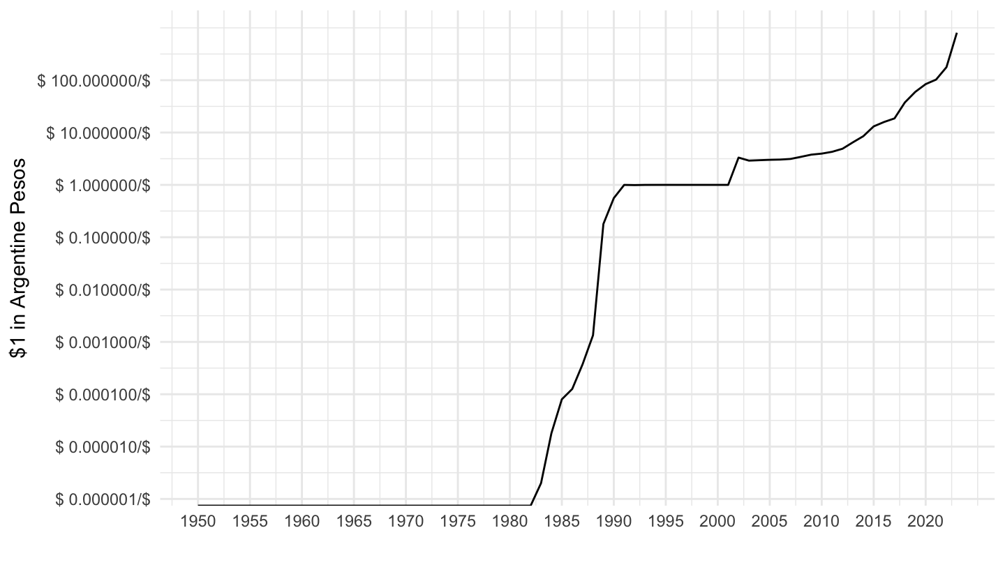
Australia, Austria, Belgium
Code
SNA_TABLE4 %>%
  filter(TRANSACT == "EXCE",
         LOCATION %in% c("AUS", "AUT", "BEL")) %>%
  left_join(SNA_TABLE4_var$LOCATION, by = "LOCATION") %>%
  left_join(colors, by = c("Location" = "country")) %>%
  year_to_date() %>%
  ggplot(.) + theme_minimal() + scale_color_identity() +
  geom_line(aes(x = date, y = obsValue, color = color)) +
  add_3flags + xlab("") + ylab("Exchange Rate ($1 = ? National Currency)") +
  scale_x_date(breaks = seq(1940, 2020, 5) %>% paste0("-01-01") %>% as.Date,
               labels = date_format("%Y")) +
  scale_y_log10(breaks = seq(0, 10, 0.1),
                     labels = dollar_format(a = 0.1, p = "", su = " ../$"))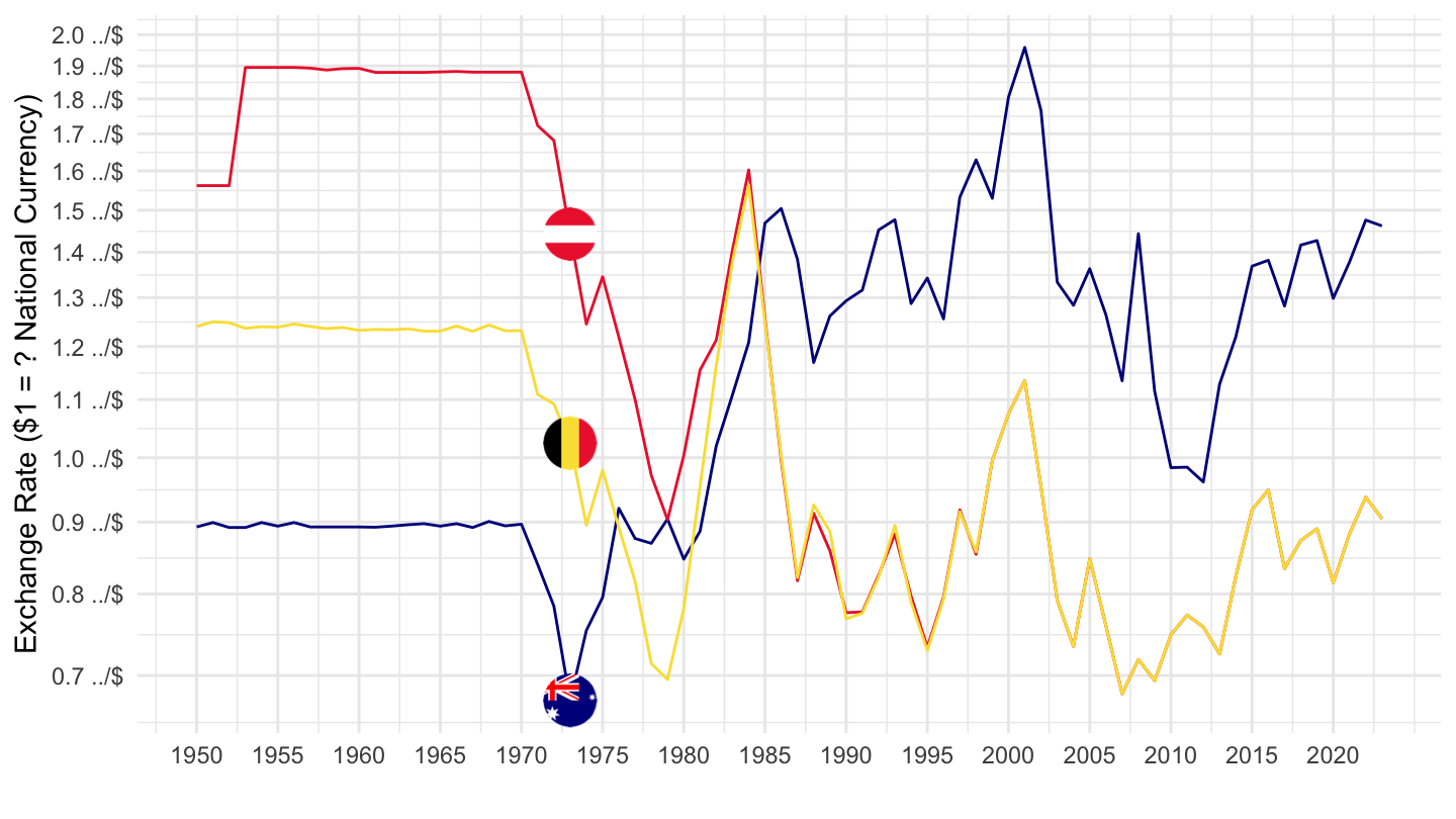
Individual Countries
Australia
Code
SNA_TABLE4 %>%
  filter(TRANSACT %in% c("PPPGDP", "PPPPRC", "PPPP41", "EXC"),
         LOCATION %in% c("AUS")) %>%
  year_to_date() %>%
  group_by(date) %>%
  mutate(obsValue = obsValue/obsValue[TRANSACT == "EXC"]) %>%
  filter(TRANSACT != "EXC") %>%
  left_join(SNA_TABLE4_var$TRANSACT, by = "TRANSACT") %>%
  ggplot(.) + theme_minimal() +
  geom_line(aes(x = date, y = obsValue, color = Transact, linetype = Transact)) +
  xlab("") + ylab("Purchasing Power Parity") +
  scale_x_date(breaks = seq(1940, 2020, 5) %>% paste0("-01-01") %>% as.Date,
               labels = date_format("%Y")) +
  scale_y_log10(breaks = seq(0, 2, 0.1)) +
  scale_color_manual(values = viridis(4)[1:3]) +
  theme(legend.position = c(0.4, 0.85),
        legend.title = element_blank())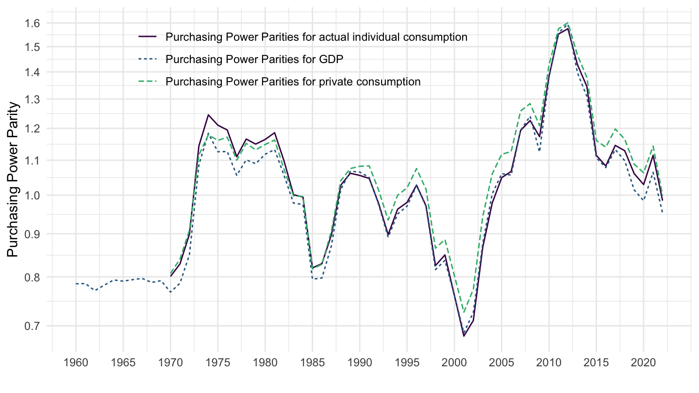
Austria
Code
SNA_TABLE4 %>%
  filter(TRANSACT %in% c("PPPGDP", "PPPPRC", "PPPP41", "EXC"),
         LOCATION %in% c("AUT")) %>%
  year_to_date() %>%
  group_by(date) %>%
  mutate(obsValue = obsValue/obsValue[TRANSACT == "EXC"]) %>%
  filter(TRANSACT != "EXC") %>%
  left_join(SNA_TABLE4_var$TRANSACT, by = "TRANSACT") %>%
  ggplot(.) + theme_minimal() +
  geom_line(aes(x = date, y = obsValue, color = Transact, linetype = Transact)) +
  xlab("") + ylab("Purchasing Power Parity") +
  scale_x_date(breaks = seq(1940, 2020, 5) %>% paste0("-01-01") %>% as.Date,
               labels = date_format("%Y")) +
  scale_y_log10(breaks = seq(0, 2, 0.1)) +
  scale_color_manual(values = viridis(4)[1:3]) +
  theme(legend.position = c(0.4, 0.85),
        legend.title = element_blank())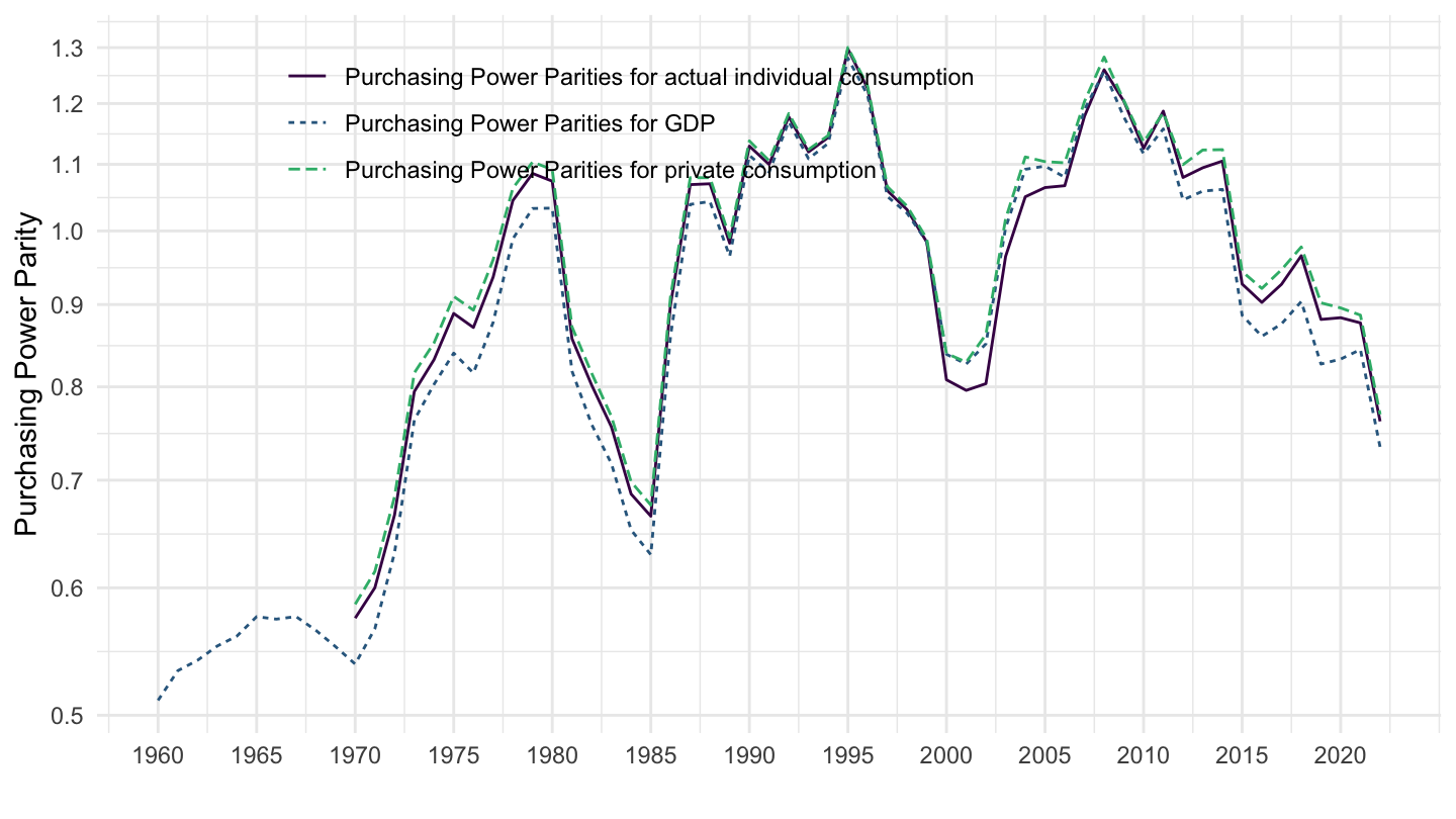
France
Code
SNA_TABLE4 %>%
  filter(TRANSACT %in% c("PPPGDP", "PPPPRC", "PPPP41", "EXC"),
         LOCATION %in% c("FRA")) %>%
  year_to_date() %>%
  group_by(date) %>%
  mutate(obsValue = obsValue/obsValue[TRANSACT == "EXC"]) %>%
  filter(TRANSACT != "EXC") %>%
  left_join(SNA_TABLE4_var$TRANSACT, by = "TRANSACT") %>%
  ggplot(.) + theme_minimal() +
  geom_line(aes(x = date, y = obsValue, color = Transact, linetype = Transact)) +
  xlab("") + ylab("Purchasing Power Parity") +
  scale_x_date(breaks = seq(1940, 2020, 5) %>% paste0("-01-01") %>% as.Date,
               labels = date_format("%Y")) +
  scale_y_log10(breaks = seq(0, 2, 0.1)) +
  scale_color_manual(values = viridis(4)[1:3]) +
  theme(legend.position = c(0.4, 0.85),
        legend.title = element_blank())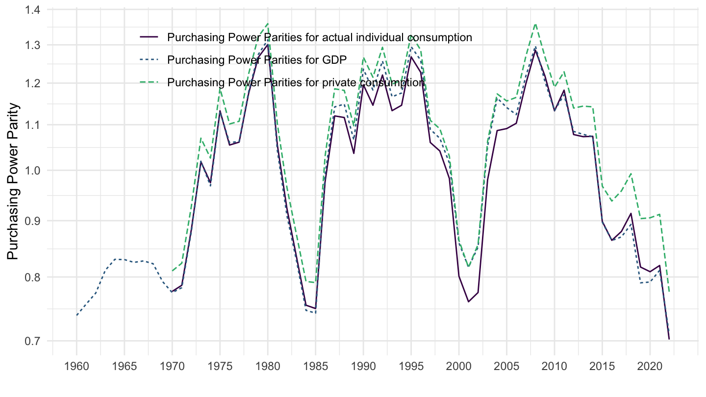
Germany
Code
SNA_TABLE4 %>%
  filter(TRANSACT %in% c("PPPGDP", "PPPPRC", "PPPP41", "EXC"),
         LOCATION %in% c("DEU")) %>%
  year_to_date() %>%
  group_by(date) %>%
  mutate(obsValue = obsValue/obsValue[TRANSACT == "EXC"]) %>%
  filter(TRANSACT != "EXC") %>%
  left_join(SNA_TABLE4_var$TRANSACT, by = "TRANSACT") %>%
  ggplot(.) + theme_minimal() +
  geom_line(aes(x = date, y = obsValue, color = Transact, linetype = Transact)) +
  xlab("") + ylab("Purchasing Power Parity") +
  scale_x_date(breaks = seq(1940, 2020, 5) %>% paste0("-01-01") %>% as.Date,
               labels = date_format("%Y")) +
  scale_y_log10(breaks = seq(0, 2, 0.1)) +
  scale_color_manual(values = viridis(4)[1:3]) +
  theme(legend.position = c(0.4, 0.85),
        legend.title = element_blank())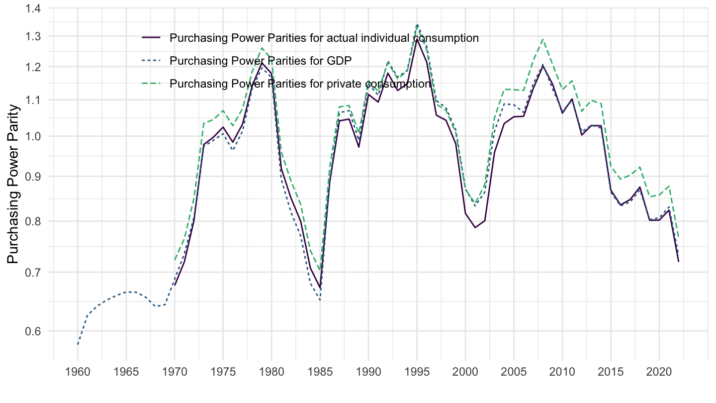
Japan
Code
SNA_TABLE4 %>%
  filter(TRANSACT %in% c("PPPGDP", "PPPPRC", "PPPP41", "EXC"),
         LOCATION %in% c("JPN")) %>%
  year_to_date() %>%
  group_by(date) %>%
  mutate(obsValue = obsValue/obsValue[TRANSACT == "EXC"]) %>%
  filter(TRANSACT != "EXC") %>%
  left_join(SNA_TABLE4_var$TRANSACT, by = "TRANSACT") %>%
  ggplot(.) + theme_minimal() +
  geom_line(aes(x = date, y = obsValue, color = Transact, linetype = Transact)) +
  xlab("") + ylab("Purchasing Power Parity") +
  scale_x_date(breaks = seq(1940, 2020, 5) %>% paste0("-01-01") %>% as.Date,
               labels = date_format("%Y")) +
  scale_y_log10(breaks = seq(0, 2, 0.1)) +
  scale_color_manual(values = viridis(4)[1:3]) +
  theme(legend.position = c(0.6, 0.15),
        legend.title = element_blank())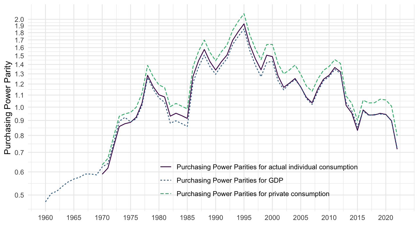
United States
Code
SNA_TABLE4 %>%
  filter(TRANSACT %in% c("PPPGDP", "PPPPRC", "PPPP41", "EXC"),
         LOCATION %in% c("USA")) %>%
  year_to_date() %>%
  group_by(date) %>%
  mutate(obsValue = obsValue/obsValue[TRANSACT == "EXC"]) %>%
  filter(TRANSACT != "EXC") %>%
  left_join(SNA_TABLE4_var$TRANSACT, by = "TRANSACT") %>%
  ggplot(.) + theme_minimal() +
  geom_line(aes(x = date, y = obsValue, color = Transact, linetype = Transact)) +
  xlab("") + ylab("Purchasing Power Parity") +
  scale_x_date(breaks = seq(1940, 2020, 5) %>% paste0("-01-01") %>% as.Date,
               labels = date_format("%Y")) +
  scale_y_log10(breaks = seq(0, 2, 0.1)) +
  scale_color_manual(values = viridis(4)[1:3]) +
  theme(legend.position = c(0.6, 0.15),
        legend.title = element_blank())
PPPGDP/EXC - Purchasing Power Parities for GDP
Table - Relative to U.S.
Javascript
Code
SNA_TABLE4 %>%
  filter(TRANSACT %in% c("PPPGDP", "EXC")) %>%
  left_join(SNA_TABLE4_var$LOCATION, by = "LOCATION") %>%
  select(LOCATION, Location, TRANSACT, obsTime, obsValue) %>%
  spread(TRANSACT, obsValue) %>%
  na.omit %>%
  group_by(LOCATION, Location) %>%
  summarise(`First Year` = first(obsTime),
            `Last Year` = last(obsTime),
            `Last PPP` = round(last(PPPGDP/EXC),2),
            Nobs = n()) %>%
  arrange(-Nobs) %>%
  {if (is_html_output()) datatable(., filter = 'top', rownames = F) else .}
png
Code
include_graphics3b("bib/oecd/SNA_TABLE4_ex2.png")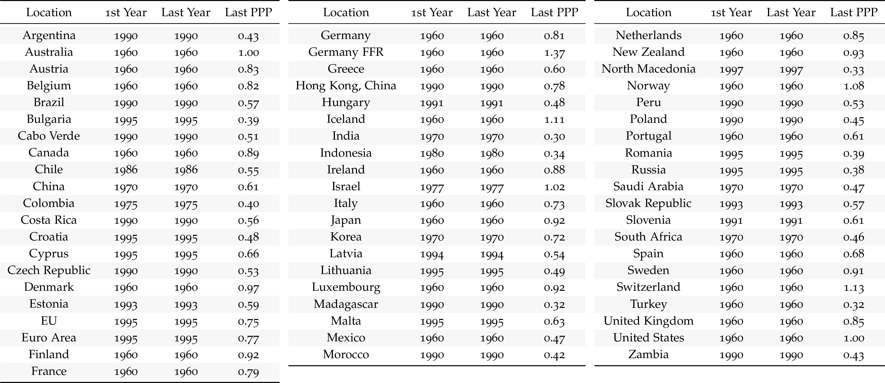
United States
Code
SNA_TABLE4 %>%
  filter(TRANSACT %in% c("PPPGDP", "EXC"),
         LOCATION %in% c("USA")) %>%
  year_to_date() %>%
  left_join(SNA_TABLE4_var$LOCATION, by = "LOCATION") %>%
  select(LOCATION, Location, date, TRANSACT, obsValue) %>%
  spread(TRANSACT, obsValue) %>%
  na.omit %>%
  ggplot(.) + theme_minimal() +
  geom_line(aes(x = date, y = PPPGDP/EXC)) +
  xlab("") + ylab("Purchasing Power Parity") +
  scale_x_date(breaks = seq(1940, 2020, 5) %>% paste0("-01-01") %>% as.Date,
               labels = date_format("%Y")) +
  scale_y_log10(breaks = seq(0, 2, 0.1)) +
  scale_color_manual(values = viridis(4)[1:3]) +
  theme(legend.position = c(0.15, 0.85),
        legend.title = element_blank())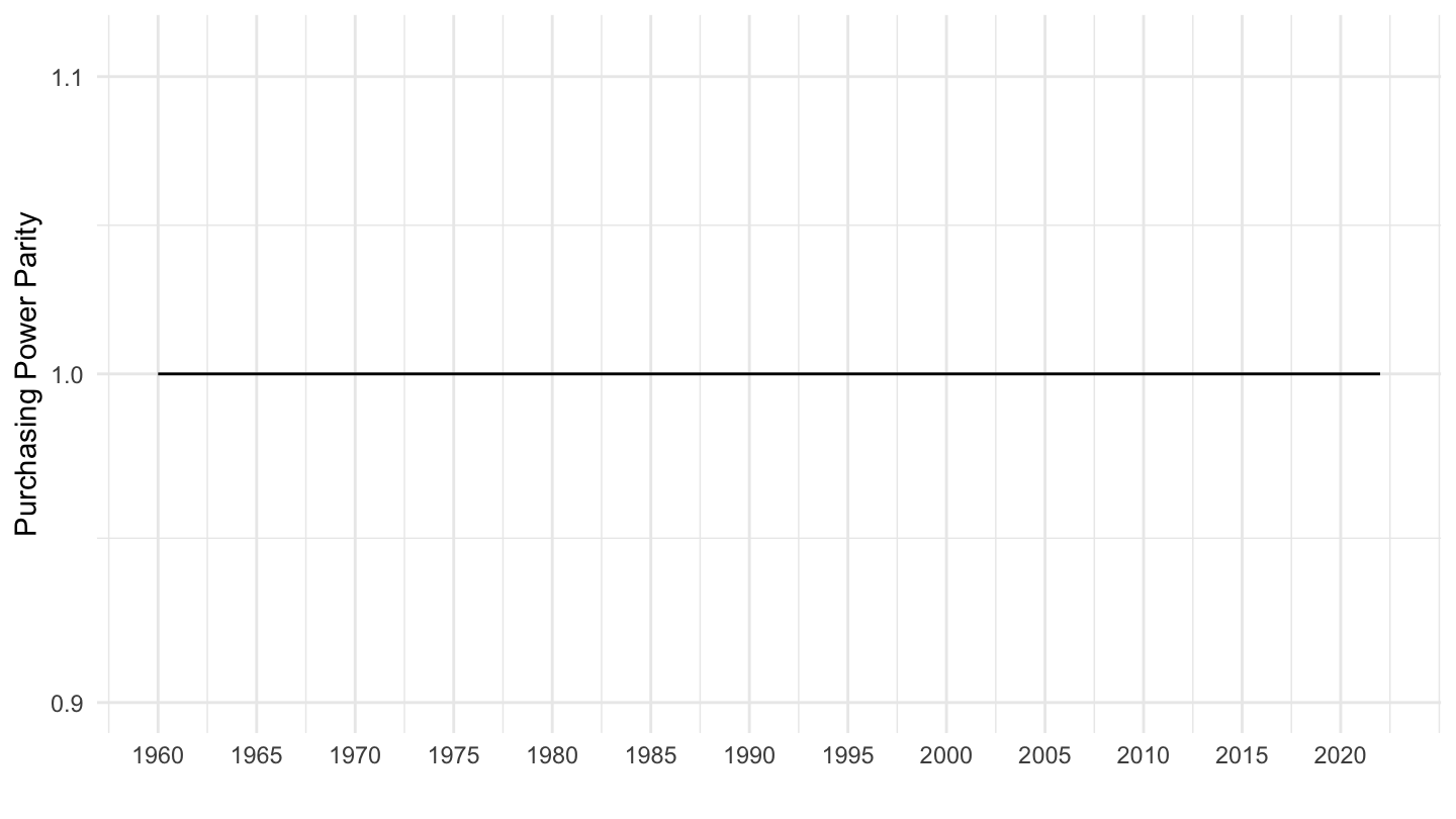
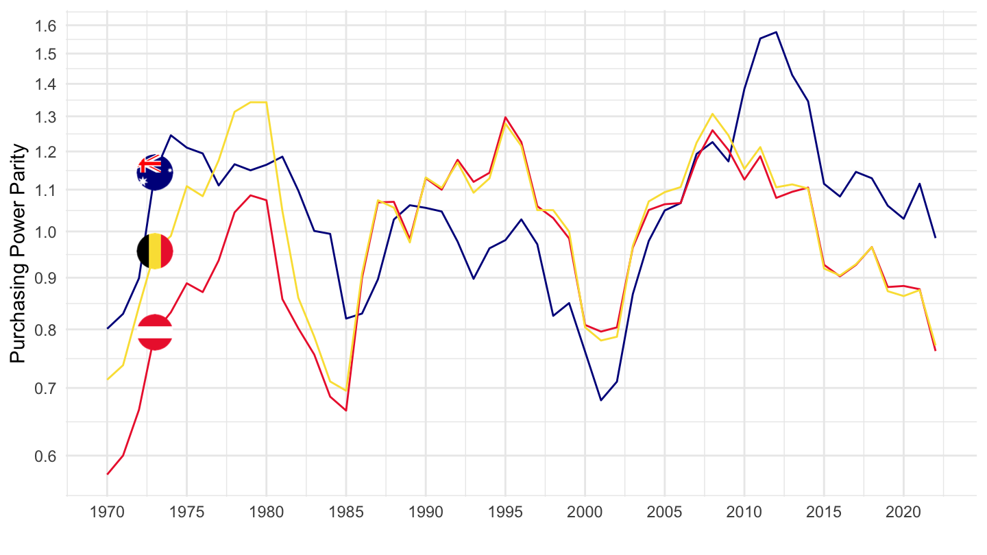
Australia, Austria, Belgium
Code
SNA_TABLE4 %>%
  filter(TRANSACT %in% c("PPPGDP", "EXC"),
         LOCATION %in% c("AUS", "AUT", "BEL")) %>%
  year_to_date() %>%
  left_join(SNA_TABLE4_var$LOCATION, by = "LOCATION") %>%
  select(LOCATION, Location, date, TRANSACT, obsValue) %>%
  spread(TRANSACT, obsValue) %>%
  mutate(obsValue = PPPGDP/EXC) %>%
  left_join(colors, by = c("Location" = "country")) %>%
  na.omit %>%
  ggplot(.) + theme_minimal() + scale_color_identity() +
  geom_line(aes(x = date, y = obsValue, color = color)) +
  xlab("") + ylab("Purchasing Power Parity") + add_3flags +
  scale_x_date(breaks = seq(1940, 2020, 5) %>% paste0("-01-01") %>% as.Date,
               labels = date_format("%Y")) +
  scale_y_log10(breaks = seq(0, 2, 0.1))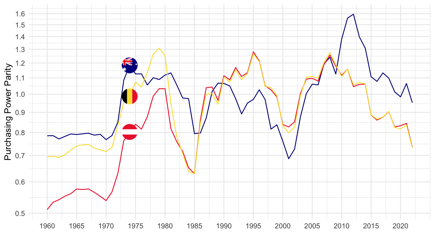
Canada, US, Germany
Code
SNA_TABLE4 %>%
  filter(TRANSACT %in% c("PPPGDP", "EXC"),
         LOCATION %in% c("CAN", "USA", "DEU")) %>%
  year_to_date() %>%
  left_join(SNA_TABLE4_var$LOCATION, by = "LOCATION") %>%
  select(LOCATION, Location, date, TRANSACT, obsValue) %>%
  spread(TRANSACT, obsValue) %>%
  mutate(obsValue = PPPGDP/EXC) %>%
  left_join(colors, by = c("Location" = "country")) %>%
  na.omit %>%
  ggplot(.) + theme_minimal() + scale_color_identity() +
  geom_line(aes(x = date, y = obsValue, color = color)) +
  xlab("") + ylab("Purchasing Power Parity") + add_3flags +
  scale_x_date(breaks = seq(1940, 2020, 5) %>% paste0("-01-01") %>% as.Date,
               labels = date_format("%Y")) +
  scale_y_log10(breaks = seq(0, 2, 0.1))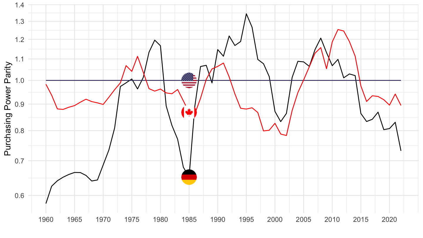
Switzerland, Germany, France
Code
SNA_TABLE4 %>%
  filter(TRANSACT %in% c("PPPGDP", "EXC"),
         LOCATION %in% c("CHE", "DEU", "FRA")) %>%
  year_to_date() %>%
  left_join(SNA_TABLE4_var$LOCATION, by = "LOCATION") %>%
  select(LOCATION, Location, date, TRANSACT, obsValue) %>%
  spread(TRANSACT, obsValue) %>%
  mutate(obsValue = PPPGDP/EXC) %>%
  left_join(colors, by = c("Location" = "country")) %>%
  na.omit %>%
  ggplot(.) + theme_minimal() + scale_color_identity() +
  geom_line(aes(x = date, y = obsValue, color = color)) +
  xlab("") + ylab("Purchasing Power Parity") + add_3flags +
  scale_x_date(breaks = seq(1940, 2020, 5) %>% paste0("-01-01") %>% as.Date,
               labels = date_format("%Y")) +
  scale_y_log10(breaks = seq(0, 2, 0.1))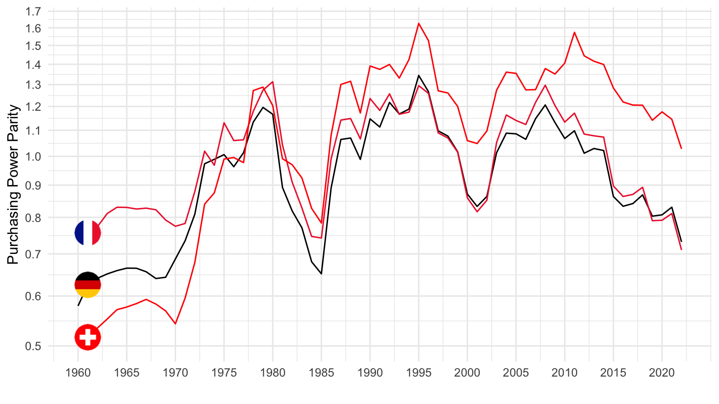
Denmark, Spain, Finland
Code
SNA_TABLE4 %>%
  filter(TRANSACT %in% c("PPPGDP", "EXC"),
         LOCATION %in% c("DNK", "ESP", "FIN")) %>%
  year_to_date() %>%
  left_join(SNA_TABLE4_var$LOCATION, by = "LOCATION") %>%
  select(LOCATION, Location, date, TRANSACT, obsValue) %>%
  spread(TRANSACT, obsValue) %>%
  mutate(obsValue = PPPGDP/EXC) %>%
  left_join(colors, by = c("Location" = "country")) %>%
  na.omit %>%
  ggplot(.) + theme_minimal() + scale_color_identity() +
  geom_line(aes(x = date, y = obsValue, color = color)) +
  xlab("") + ylab("Purchasing Power Parity") + add_3flags +
  scale_x_date(breaks = seq(1940, 2020, 5) %>% paste0("-01-01") %>% as.Date,
               labels = date_format("%Y")) +
  scale_y_log10(breaks = seq(0, 2, 0.1))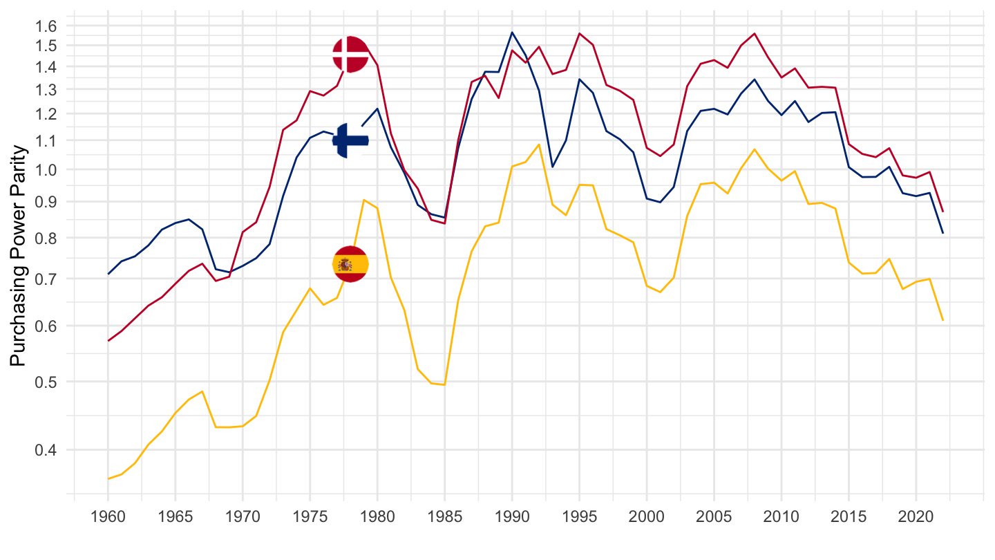
France, Greece, United Kingdom
Code
SNA_TABLE4 %>%
  filter(TRANSACT %in% c("PPPGDP", "EXC"),
         LOCATION %in% c("FRA", "GBR", "GRC")) %>%
  year_to_date() %>%
  left_join(SNA_TABLE4_var$LOCATION, by = "LOCATION") %>%
  select(LOCATION, Location, date, TRANSACT, obsValue) %>%
  spread(TRANSACT, obsValue) %>%
  mutate(obsValue = PPPGDP/EXC) %>%
  left_join(colors, by = c("Location" = "country")) %>%
  na.omit %>%
  ggplot(.) + theme_minimal() + scale_color_identity() +
  geom_line(aes(x = date, y = obsValue, color = color)) +
  xlab("") + ylab("Purchasing Power Parity") + add_3flags +
  scale_x_date(breaks = seq(1940, 2020, 5) %>% paste0("-01-01") %>% as.Date,
               labels = date_format("%Y")) +
  scale_y_log10(breaks = seq(0, 2, 0.1))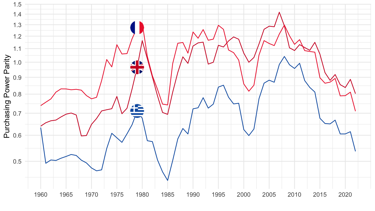
Iceland, Ireland, Italy
Code
SNA_TABLE4 %>%
  filter(TRANSACT %in% c("PPPGDP", "EXC"),
         LOCATION %in% c("IRL", "ISL", "ITA")) %>%
  year_to_date() %>%
  left_join(SNA_TABLE4_var$LOCATION, by = "LOCATION") %>%
  select(LOCATION, Location, date, TRANSACT, obsValue) %>%
  spread(TRANSACT, obsValue) %>%
  mutate(obsValue = PPPGDP/EXC) %>%
  left_join(colors, by = c("Location" = "country")) %>%
  na.omit %>%
  ggplot(.) + theme_minimal() + scale_color_identity() +
  geom_line(aes(x = date, y = obsValue, color = color)) +
  xlab("") + ylab("Purchasing Power Parity") + add_3flags +
  scale_x_date(breaks = seq(1940, 2020, 5) %>% paste0("-01-01") %>% as.Date,
               labels = date_format("%Y")) +
  scale_y_log10(breaks = seq(0, 2, 0.1))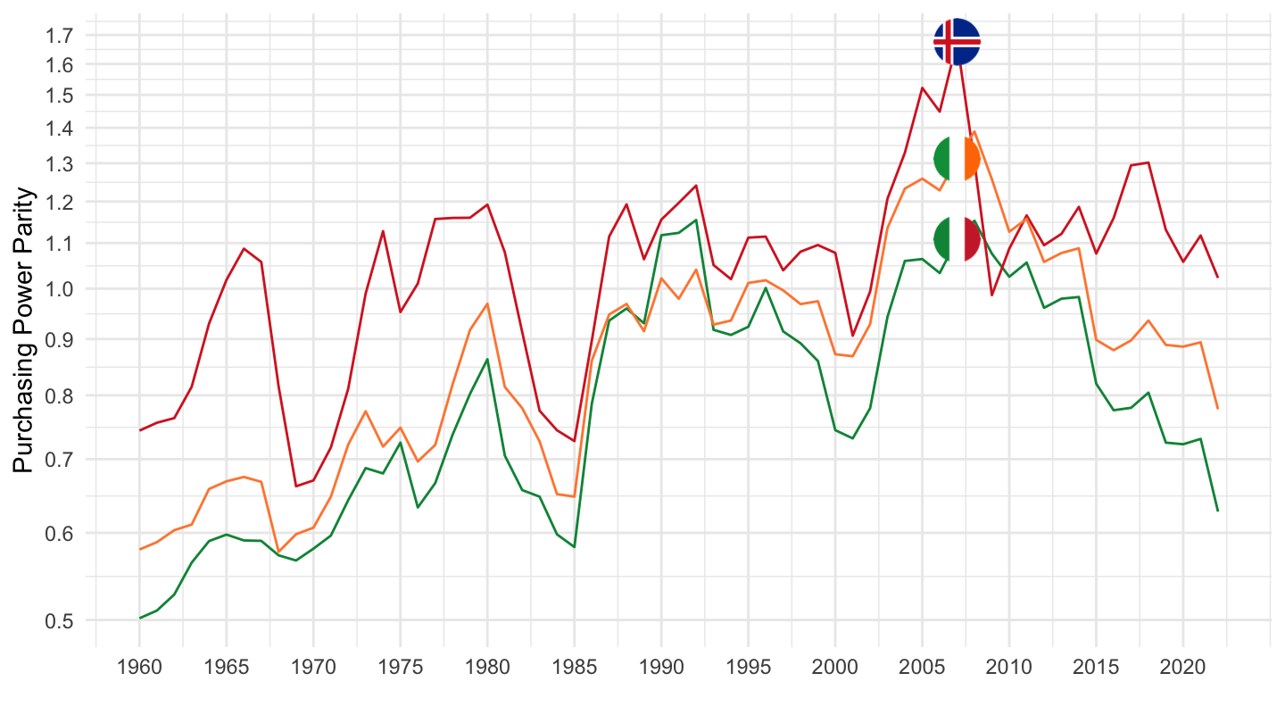
Japan, Luxembourg, Mexico
Code
SNA_TABLE4 %>%
  filter(TRANSACT %in% c("PPPGDP", "EXC"),
         LOCATION %in% c("JPN", "LUX", "MEX")) %>%
  year_to_date() %>%
  left_join(SNA_TABLE4_var$LOCATION, by = "LOCATION") %>%
  select(LOCATION, Location, date, TRANSACT, obsValue) %>%
  spread(TRANSACT, obsValue) %>%
  mutate(obsValue = PPPGDP/EXC) %>%
  left_join(colors, by = c("Location" = "country")) %>%
  na.omit %>%
  ggplot(.) + theme_minimal() + scale_color_identity() +
  geom_line(aes(x = date, y = obsValue, color = color)) +
  xlab("") + ylab("Purchasing Power Parity") + add_3flags +
  scale_x_date(breaks = seq(1940, 2020, 5) %>% paste0("-01-01") %>% as.Date,
               labels = date_format("%Y")) +
  scale_y_log10(breaks = seq(0, 2, 0.1))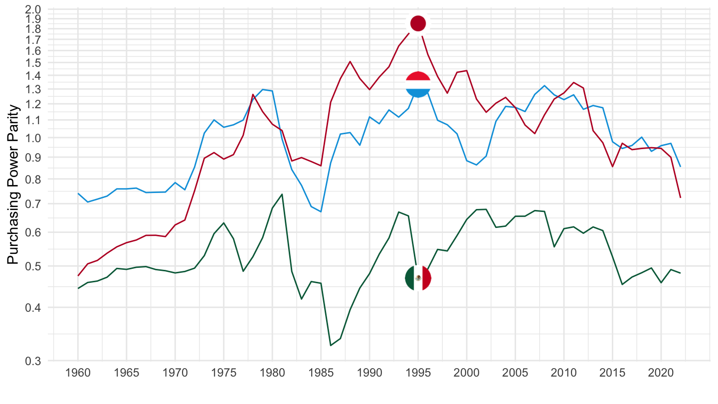
Netherlands, Norway, New Zealand
Code
SNA_TABLE4 %>%
  filter(TRANSACT %in% c("PPPGDP", "EXC"),
         LOCATION %in% c("NLD", "NOR", "NZL")) %>%
  year_to_date() %>%
  left_join(SNA_TABLE4_var$LOCATION, by = "LOCATION") %>%
  select(LOCATION, Location, date, TRANSACT, obsValue) %>%
  spread(TRANSACT, obsValue) %>%
  mutate(obsValue = PPPGDP/EXC) %>%
  left_join(colors, by = c("Location" = "country")) %>%
  na.omit %>%
  ggplot(.) + theme_minimal() + scale_color_identity() +
  geom_line(aes(x = date, y = obsValue, color = color)) +
  xlab("") + ylab("Purchasing Power Parity") + add_3flags +
  scale_x_date(breaks = seq(1940, 2020, 5) %>% paste0("-01-01") %>% as.Date,
               labels = date_format("%Y")) +
  scale_y_log10(breaks = seq(0, 2, 0.1))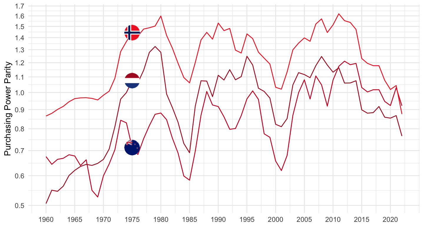
Portugal, Sweden, Turkey
Code
SNA_TABLE4 %>%
  filter(TRANSACT %in% c("PPPGDP", "EXC"),
         LOCATION %in% c("PRT", "SWE", "TUR")) %>%
  year_to_date() %>%
  left_join(SNA_TABLE4_var$LOCATION, by = "LOCATION") %>%
  select(LOCATION, Location, date, TRANSACT, obsValue) %>%
  spread(TRANSACT, obsValue) %>%
  mutate(obsValue = PPPGDP/EXC) %>%
  left_join(colors, by = c("Location" = "country")) %>%
  na.omit %>%
  ggplot(.) + theme_minimal() + scale_color_identity() +
  geom_line(aes(x = date, y = obsValue, color = color)) +
  xlab("") + ylab("Purchasing Power Parity") + add_3flags +
  scale_x_date(breaks = seq(1940, 2020, 5) %>% paste0("-01-01") %>% as.Date,
               labels = date_format("%Y")) +
  scale_y_log10(breaks = seq(0, 2, 0.1))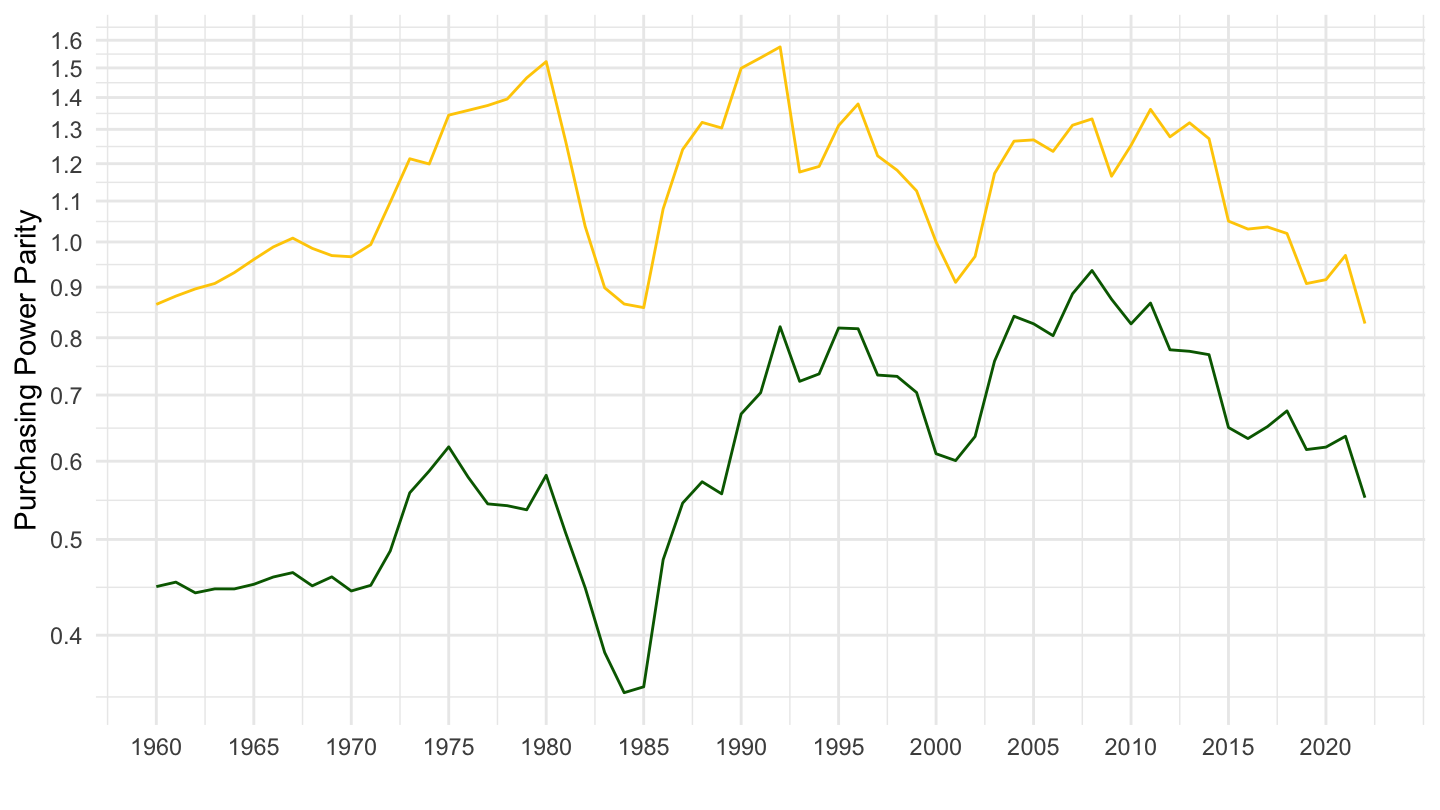
China, India, Korea
Code
SNA_TABLE4 %>%
  filter(TRANSACT %in% c("PPPGDP", "EXC"),
         LOCATION %in% c("CHN", "IND", "KOR")) %>%
  year_to_date() %>%
  left_join(SNA_TABLE4_var$LOCATION, by = "LOCATION") %>%
  select(LOCATION, Location, date, TRANSACT, obsValue) %>%
  spread(TRANSACT, obsValue) %>%
  mutate(obsValue = PPPGDP/EXC) %>%
  left_join(colors, by = c("Location" = "country")) %>%
  na.omit %>%
  ggplot(.) + theme_minimal() + scale_color_identity() +
  geom_line(aes(x = date, y = obsValue, color = color)) +
  xlab("") + ylab("Purchasing Power Parity") + add_3flags +
  scale_x_date(breaks = seq(1940, 2020, 5) %>% paste0("-01-01") %>% as.Date,
               labels = date_format("%Y")) +
  scale_y_log10(breaks = seq(0, 2, 0.1))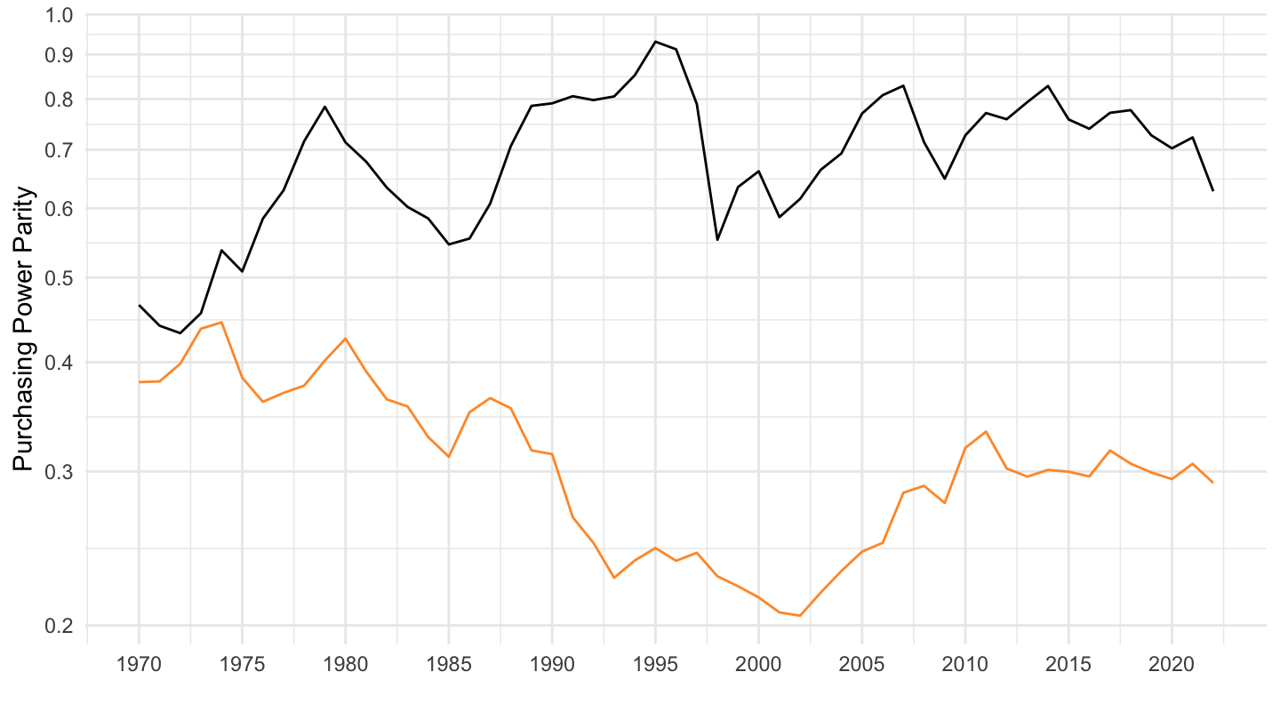
Saudi Arabia, South Africa, Colombia
Code
SNA_TABLE4 %>%
  filter(TRANSACT %in% c("PPPGDP", "EXC"),
         LOCATION %in% c("SAU", "ZAF", "COL")) %>%
  year_to_date() %>%
  left_join(SNA_TABLE4_var$LOCATION, by = "LOCATION") %>%
  select(LOCATION, Location, date, TRANSACT, obsValue) %>%
  spread(TRANSACT, obsValue) %>%
  mutate(obsValue = PPPGDP/EXC) %>%
  left_join(colors, by = c("Location" = "country")) %>%
  na.omit %>%
  ggplot(.) + theme_minimal() + scale_color_identity() +
  geom_line(aes(x = date, y = obsValue, color = color)) +
  xlab("") + ylab("Purchasing Power Parity") + add_3flags +
  scale_x_date(breaks = seq(1940, 2020, 5) %>% paste0("-01-01") %>% as.Date,
               labels = date_format("%Y")) +
  scale_y_log10(breaks = seq(0, 2, 0.1))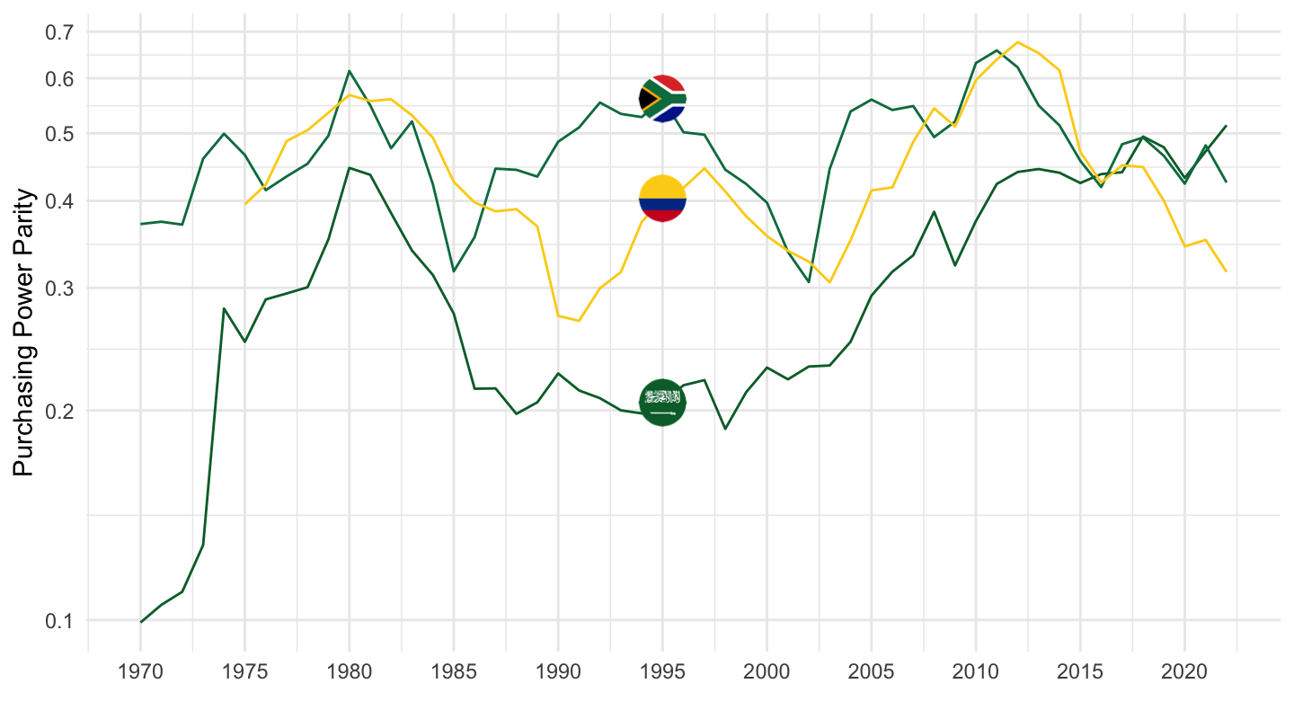
Israel, Indonesia, Germany FFR
Code
SNA_TABLE4 %>%
  filter(TRANSACT %in% c("PPPGDP", "EXC"),
         LOCATION %in% c("ISR", "IDN", "DEW")) %>%
  year_to_date() %>%
  left_join(SNA_TABLE4_var$LOCATION, by = "LOCATION") %>%
  select(LOCATION, Location, date, TRANSACT, obsValue) %>%
  spread(TRANSACT, obsValue) %>%
  mutate(obsValue = PPPGDP/EXC) %>%
  left_join(colors, by = c("Location" = "country")) %>%
  na.omit %>%
  ggplot(.) + theme_minimal() + scale_color_identity() +
  geom_line(aes(x = date, y = obsValue, color = color)) +
  xlab("") + ylab("Purchasing Power Parity") + add_3flags +
  scale_x_date(breaks = seq(1940, 2020, 5) %>% paste0("-01-01") %>% as.Date,
               labels = date_format("%Y")) +
  scale_y_log10(breaks = seq(0, 2, 0.1))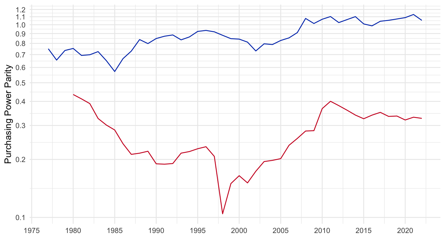
Chile, Argentina, Brazil
Code
SNA_TABLE4 %>%
  filter(TRANSACT %in% c("PPPGDP", "EXC"),
         LOCATION %in% c("CHL", "ARG", "BRA")) %>%
  year_to_date() %>%
  left_join(SNA_TABLE4_var$LOCATION, by = "LOCATION") %>%
  select(LOCATION, Location, date, TRANSACT, obsValue) %>%
  spread(TRANSACT, obsValue) %>%
  mutate(obsValue = PPPGDP/EXC) %>%
  left_join(colors, by = c("Location" = "country")) %>%
  na.omit %>%
  ggplot(.) + theme_minimal() + scale_color_identity() +
  geom_line(aes(x = date, y = obsValue, color = color)) +
  xlab("") + ylab("Purchasing Power Parity") + add_3flags +
  scale_x_date(breaks = seq(1940, 2020, 5) %>% paste0("-01-01") %>% as.Date,
               labels = date_format("%Y")) +
  scale_y_log10(breaks = seq(0, 2, 0.1))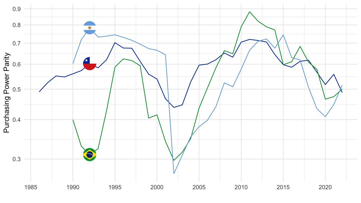
Costa Rica, Czech Republic, Poland
Code
SNA_TABLE4 %>%
  filter(TRANSACT %in% c("PPPGDP", "EXC"),
         LOCATION %in% c("CRI", "CZE", "POL")) %>%
  year_to_date() %>%
  left_join(SNA_TABLE4_var$LOCATION, by = "LOCATION") %>%
  select(LOCATION, Location, date, TRANSACT, obsValue) %>%
  spread(TRANSACT, obsValue) %>%
  mutate(obsValue = PPPGDP/EXC) %>%
  left_join(colors, by = c("Location" = "country")) %>%
  na.omit %>%
  ggplot(.) + theme_minimal() + scale_color_identity() +
  geom_line(aes(x = date, y = obsValue, color = color)) +
  xlab("") + ylab("Purchasing Power Parity") + add_3flags +
  scale_x_date(breaks = seq(1940, 2020, 5) %>% paste0("-01-01") %>% as.Date,
               labels = date_format("%Y")) +
  scale_y_log10(breaks = seq(0, 2, 0.1))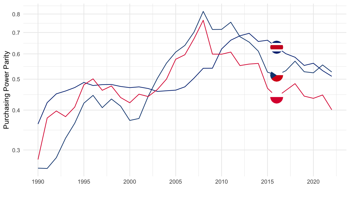
Cabo Verde, Hong Kong, China, Hungary
Code
SNA_TABLE4 %>%
  filter(TRANSACT %in% c("PPPGDP", "EXC"),
         LOCATION %in% c("CPV", "HKG", "HUN")) %>%
  year_to_date() %>%
  left_join(SNA_TABLE4_var$LOCATION, by = "LOCATION") %>%
  select(LOCATION, Location, date, TRANSACT, obsValue) %>%
  spread(TRANSACT, obsValue) %>%
  mutate(obsValue = PPPGDP/EXC) %>%
  left_join(colors, by = c("Location" = "country")) %>%
  na.omit %>%
  ggplot(.) + theme_minimal() + scale_color_identity() +
  geom_line(aes(x = date, y = obsValue, color = color)) +
  xlab("") + ylab("Purchasing Power Parity") + add_3flags +
  scale_x_date(breaks = seq(1940, 2020, 5) %>% paste0("-01-01") %>% as.Date,
               labels = date_format("%Y")) +
  scale_y_log10(breaks = seq(0, 2, 0.1))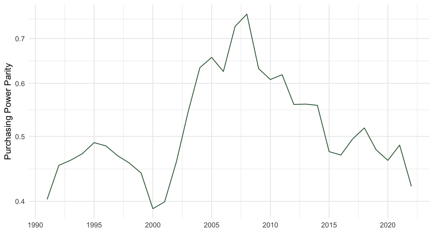
Morocco, Madagascar, Peru
Code
SNA_TABLE4 %>%
  filter(TRANSACT %in% c("PPPGDP", "EXC"),
         LOCATION %in% c("MAR", "MDG", "PER")) %>%
  year_to_date() %>%
  left_join(SNA_TABLE4_var$LOCATION, by = "LOCATION") %>%
  select(LOCATION, Location, date, TRANSACT, obsValue) %>%
  spread(TRANSACT, obsValue) %>%
  mutate(obsValue = PPPGDP/EXC) %>%
  left_join(colors, by = c("Location" = "country")) %>%
  na.omit %>%
  ggplot(.) + theme_minimal() + scale_color_identity() +
  geom_line(aes(x = date, y = obsValue, color = color)) +
  xlab("") + ylab("Purchasing Power Parity") + add_3flags +
  scale_x_date(breaks = seq(1940, 2020, 5) %>% paste0("-01-01") %>% as.Date,
               labels = date_format("%Y")) +
  scale_y_log10(breaks = seq(0, 2, 0.1))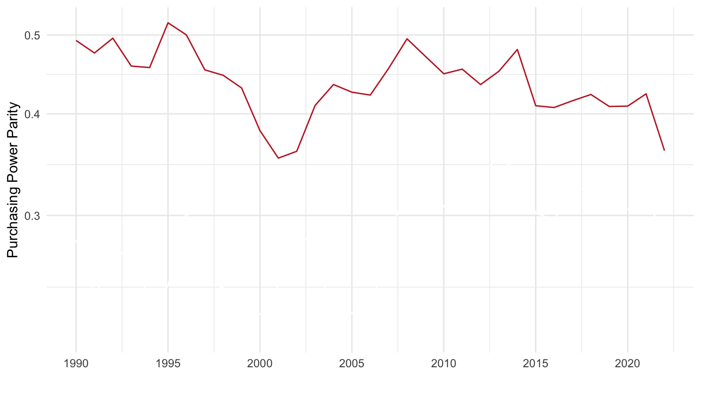
PPPPRC - Purchasing Power Parities for private consumption
Table
Code
SNA_TABLE4 %>%
  filter(TRANSACT %in% c("PPPPRC", "EXC")) %>%
  left_join(SNA_TABLE4_var$LOCATION, by = "LOCATION") %>%
  select(LOCATION, Location, TRANSACT, obsTime, obsValue) %>%
  spread(TRANSACT, obsValue) %>%
  na.omit %>%
  group_by(LOCATION, Location) %>%
  summarise(`First Year` = first(obsTime),
            `Last Year` = last(obsTime),
            `Last PPP` = round(last(PPPPRC/EXC),2),
            Nobs = n()) %>%
  arrange(-Nobs) %>%
  {if (is_html_output()) datatable(., filter = 'top', rownames = F) else .}
Australia, Austria, Belgium
Code
SNA_TABLE4 %>%
  filter(TRANSACT %in% c("PPPPRC", "EXC"),
         LOCATION %in% c("AUS", "AUT", "BEL")) %>%
  year_to_date() %>%
  left_join(SNA_TABLE4_var$LOCATION, by = "LOCATION") %>%
  select(LOCATION, Location, date, TRANSACT, obsValue) %>%
  spread(TRANSACT, obsValue) %>%
  mutate(obsValue = PPPPRC/EXC) %>%
  left_join(colors, by = c("Location" = "country")) %>%
  na.omit %>%
  ggplot(.) + theme_minimal() + scale_color_identity() +
  geom_line(aes(x = date, y = obsValue, color = color)) +
  xlab("") + ylab("Purchasing Power Parity") + add_3flags +
  scale_x_date(breaks = seq(1940, 2020, 5) %>% paste0("-01-01") %>% as.Date,
               labels = date_format("%Y")) +
  scale_y_log10(breaks = seq(0, 2, 0.1))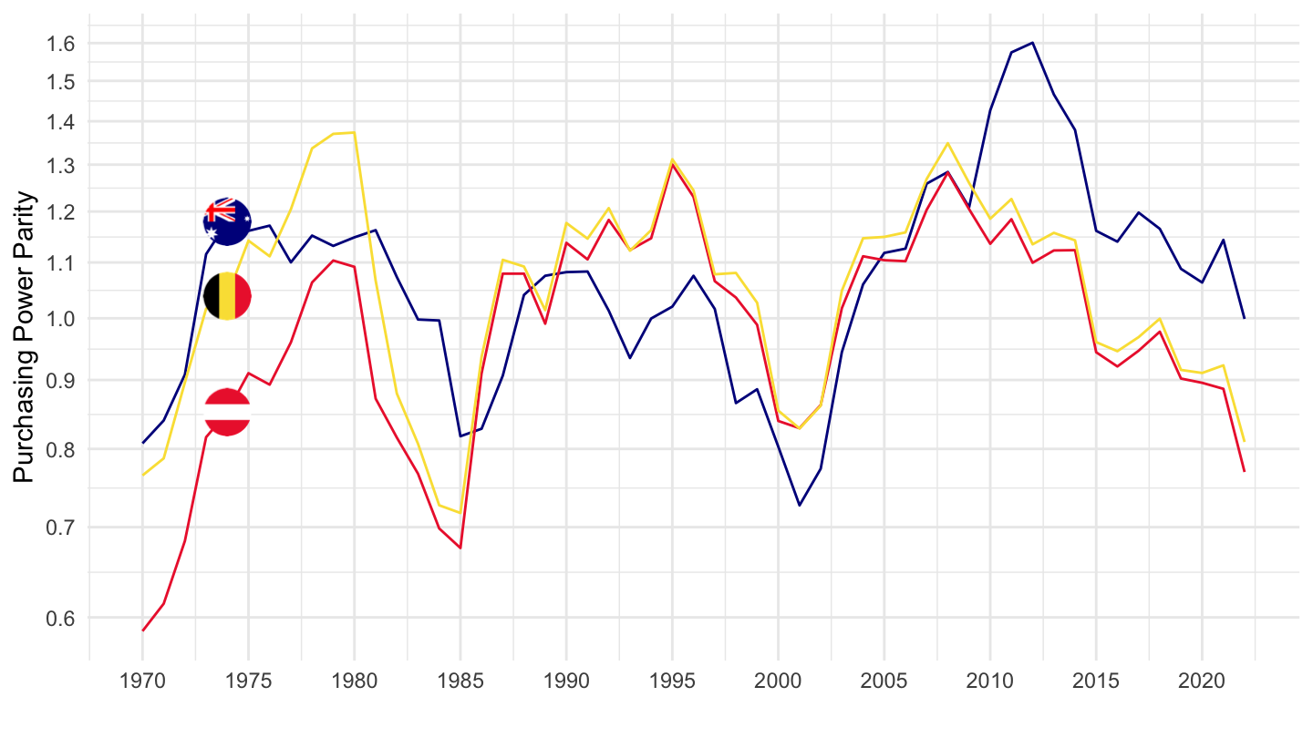
PPPP41 - Purchasing Power Parities for actual individual consumption
Table
Code
SNA_TABLE4 %>%
  filter(TRANSACT %in% c("PPPP41", "EXC")) %>%
  left_join(SNA_TABLE4_var$LOCATION, by = "LOCATION") %>%
  select(LOCATION, Location, TRANSACT, obsTime, obsValue) %>%
  spread(TRANSACT, obsValue) %>%
  na.omit %>%
  group_by(LOCATION, Location) %>%
  summarise(`First Year` = first(obsTime),
            `Last Year` = last(obsTime),
            `Last PPP` = round(last(PPPP41/EXC),2),
            Nobs = n()) %>%
  arrange(-Nobs) %>%
  {if (is_html_output()) datatable(., filter = 'top', rownames = F) else .}
Australia, Austria, Belgium
Code
SNA_TABLE4 %>%
  filter(TRANSACT %in% c("PPPP41", "EXC"),
         LOCATION %in% c("AUS", "AUT", "BEL")) %>%
  year_to_date() %>%
  left_join(SNA_TABLE4_var$LOCATION, by = "LOCATION") %>%
  select(LOCATION, Location, date, TRANSACT, obsValue) %>%
  spread(TRANSACT, obsValue) %>%
  mutate(obsValue = PPPP41/EXC) %>%
  left_join(colors, by = c("Location" = "country")) %>%
  na.omit %>%
  ggplot(.) + theme_minimal() + scale_color_identity() +
  geom_line(aes(x = date, y = obsValue, color = color)) +
  xlab("") + ylab("Purchasing Power Parity") + add_3flags +
  scale_x_date(breaks = seq(1940, 2020, 5) %>% paste0("-01-01") %>% as.Date,
               labels = date_format("%Y")) +
  scale_y_log10(breaks = seq(0, 2, 0.1))