GDP and main components (output, expenditure and income)
Data - Eurostat
Info
Last observation: Quarterly: 2026Q1 (N = 62,635)
First observation: Quarterly: 1978Q1 (N = 1,017)
Last data update: 23 jul 2026, 22:20. Last compile: 24 jul 2026, 03:00
Structure
Live
Last GDP Numbers
Instantaneous
Code
namq_10_gdp %>%
  filter(time %in% c("2021Q2", "2021Q1", "2019Q4", "2017Q2"),
         na_item == "B1GQ",
         # SCA: Seasonally and calendar adjusted data
         s_adj == "SCA",
         # CLV10_MEUR: Chain linked volumes (2010), million euro
         unit == "CLV10_MEUR") %>%

  select(geo, Geo, time, values) %>%
  spread(time, values) %>%
  mutate(`2019Q4-2021Q2` = round(100*(`2021Q2`/`2019Q4`-1), 2)) %>%
  mutate(Flag = gsub(" ", "-", str_to_lower(Geo)),
         Flag = paste0('<img src="../../icon/flag/vsmall/', Flag, '.png" alt="Flag">')) %>%
  select(Flag, everything()) %>%
  {if (is_html_output()) datatable(., filter = 'top', rownames = F, escape = F) else .}
Average
Code
namq_10_gdp %>%
  filter(na_item == "B1GQ",
         # SCA: Seasonally and calendar adjusted data
         s_adj == "SCA",
         # CLV10_MEUR: Chain linked volumes (2010), million euro
         unit == "CLV10_MEUR") %>%
  quarter_to_date %>%
  filter(date >= as.Date("2019-10-01")) %>%
  group_by(geo) %>%
  arrange(date) %>%
  mutate(values = 100*values/values[date == as.Date("2019-10-01")],
         values = cumsum(values) / seq_along(values)) %>%
  group_by(geo) %>%
  do(tail(., 1)) %>%

  select(geo, Geo, date, values) %>%
  arrange(values) %>%
  mutate(Flag = gsub(" ", "-", str_to_lower(Geo)),
         Flag = paste0('<img src="../../icon/flag/vsmall/', Flag, '.png" alt="Flag">')) %>%
  select(Flag, everything()) %>%
  {if (is_html_output()) datatable(., filter = 'top', rownames = F, escape = F) else .}
Germany, Italy, France, Spain
Table
Code
namq_10_gdp %>%
  filter(na_item == "B1GQ",
         s_adj == "SCA",
         unit == "CLV10_MEUR",
         geo %in% c("DE", "IT", "ES", "FR")) %>%
  quarter_to_date %>%
  arrange(date) %>%
  filter(date == as.Date("2019-10-01") | date == last(date)) %>%
  group_by(geo) %>%
  mutate(values = 100*values/values[1]) %>%

  select(date, geo, Geo, values) %>%
print_table_conditional()| date | geo | Geo | values |
|---|---|---|---|
| 2019-10-01 | DE | Germany | 100.0000 |
| 2019-10-01 | ES | Spain | 100.0000 |
| 2019-10-01 | FR | France | 100.0000 |
| 2019-10-01 | IT | Italy | 100.0000 |
| 2026-01-01 | DE | Germany | 100.7660 |
| 2026-01-01 | ES | Spain | 111.3231 |
| 2026-01-01 | FR | France | 106.3175 |
| 2026-01-01 | IT | Italy | 107.4317 |
Graph
Code
data <- namq_10_gdp %>%
  filter(na_item == "B1GQ",
         # SCA: Seasonally and calendar adjusted data
         s_adj == "SCA",
         # CLV10_MEUR: Chain linked volumes (2010), million euro
         unit == "CLV10_MEUR",
         geo %in% c("DE", "IT", "ES", "FR")) %>%
  quarter_to_date %>%
  filter(date >= as.Date("2019-10-01")) %>%
  group_by(geo) %>%
  arrange(date) %>%
  mutate(values = 100*values/values[1]) %>%

  left_join(colors, by = c("Geo" = "country")) %>%
  mutate(date = zoo::as.yearqtr(paste0(year(date), " Q", quarter(date))))
data %>%
  ggplot + geom_line(aes(x = date, y = values, color = color)) +
  scale_color_identity() + theme_minimal() + xlab("") + ylab("") + add_4flags +
  zoo::scale_x_yearqtr(labels = date_format("%Y Q%q"),
                       breaks = seq(min(data$date), max(data$date), by = 0.25)) +
  theme(legend.position = c(0.35, 0.85),
        legend.title = element_blank(),
        axis.text.x = element_text(angle = 45, vjust = 1, hjust = 1)) +
  scale_y_log10(breaks = seq(10, 300, 5))
Germany, France, Europe
2017T2-
Code
namq_10_gdp %>%
  filter(na_item == "B1GQ",
         # SCA: Seasonally and calendar adjusted data
         s_adj == "SCA",
         # CLV10_MEUR: Chain linked volumes (2010), million euro
         unit == "CLV10_MEUR",
         geo %in% c("DE", "EA", "FR")) %>%
  quarter_to_date %>%
  filter(date >= as.Date("2017-04-01")) %>%
  group_by(geo) %>%
  mutate(values = 100*values/values[date == as.Date("2017-04-01")]) %>%

  mutate(Geo = ifelse(geo == "EA", "Europe", Geo)) %>%
  left_join(colors, by = c("Geo" = "country")) %>%
  mutate(date = zoo::as.yearqtr(paste0(year(date), " Q", quarter(date)))) %>%
  ggplot + geom_line(aes(x = date, y = values, color = color)) + add_3flags +
  scale_color_identity() + theme_minimal() + xlab("") + ylab("PIB réel (Base 100 = 2019T4)") +
  zoo::scale_x_yearqtr(labels = date_format("%Y Q%q"),
                       breaks = seq(zoo::as.yearqtr("2017 Q2"), zoo::as.yearqtr("2100 Q1"), by = 0.25)) +
  theme(legend.position = c(0.35, 0.85),
        legend.title = element_blank(),
        axis.text.x = element_text(angle = 45, vjust = 1, hjust = 1)) +
  scale_y_log10(breaks = seq(10, 300, 2))
2019-
Code
namq_10_gdp %>%
  filter(na_item == "B1GQ",
         # SCA: Seasonally and calendar adjusted data
         s_adj == "SCA",
         # CLV10_MEUR: Chain linked volumes (2010), million euro
         unit == "CLV10_MEUR",
         geo %in% c("DE", "EA", "FR")) %>%
  quarter_to_date %>%
  filter(date >= as.Date("2019-10-01")) %>%
  group_by(geo) %>%
  mutate(values = 100*values/values[date == as.Date("2019-10-01")]) %>%

  mutate(Geo = ifelse(geo == "EA", "Europe", Geo)) %>%
  left_join(colors, by = c("Geo" = "country")) %>%
  mutate(date = zoo::as.yearqtr(paste0(year(date), " Q", quarter(date)))) %>%
  ggplot + geom_line(aes(x = date, y = values, color = color)) + add_3flags +
  scale_color_identity() + theme_minimal() + xlab("") + ylab("PIB réel (Base 100 = 2019T4)") +
  zoo::scale_x_yearqtr(labels = date_format("%Y Q%q"),
                       breaks = seq(zoo::as.yearqtr("2019 Q4"), zoo::as.yearqtr("2100 Q1"), by = 0.25)) +
  theme(legend.position = c(0.35, 0.85),
        legend.title = element_blank(),
        axis.text.x = element_text(angle = 45, vjust = 1, hjust = 1)) +
  scale_y_log10(breaks = seq(10, 300, 2))
2022-
Code
namq_10_gdp %>%
  filter(na_item == "B1GQ",
         # SCA: Seasonally and calendar adjusted data
         s_adj == "SCA",
         # CLV10_MEUR: Chain linked volumes (2010), million euro
         unit == "CLV10_MEUR",
         geo %in% c("DE", "EA", "FR")) %>%
  quarter_to_date %>%
  filter(date >= as.Date("2021-10-01")) %>%
  group_by(geo) %>%
  mutate(values = 100*values/values[date == as.Date("2021-10-01")]) %>%

  mutate(Geo = ifelse(geo == "EA", "Europe", Geo)) %>%
  left_join(colors, by = c("Geo" = "country")) %>%
  mutate(date = zoo::as.yearqtr(paste0(year(date), " Q", quarter(date)))) %>%
  ggplot + geom_line(aes(x = date, y = values, color = color)) + add_3flags +
  scale_color_identity() + theme_minimal() + xlab("") + ylab("PIB réel (Base 100 = 2019T4)") +
  zoo::scale_x_yearqtr(labels = date_format("%Y Q%q"),
                       breaks = seq(zoo::as.yearqtr("2019 Q4"), zoo::as.yearqtr("2100 Q1"), by = 0.25)) +
  theme(legend.position = c(0.35, 0.85),
        legend.title = element_blank(),
        axis.text.x = element_text(angle = 45, vjust = 1, hjust = 1)) +
  scale_y_log10(breaks = seq(10, 300, 1))
Average
Code
namq_10_gdp %>%
  filter(na_item == "B1GQ",
         # SCA: Seasonally and calendar adjusted data
         s_adj == "SCA",
         # CLV10_MEUR: Chain linked volumes (2010), million euro
         unit == "CLV10_MEUR",
         geo %in% c("DE", "EA", "FR")) %>%
  quarter_to_date %>%
  filter(date >= as.Date("2019-10-01")) %>%
  group_by(geo) %>%
  arrange(date) %>%
  mutate(values = 100*values/values[date == as.Date("2019-10-01")],
         values = cumsum(values) / seq_along(values)) %>%

  mutate(Geo = ifelse(geo == "EA", "Europe", Geo)) %>%
  left_join(colors, by = c("Geo" = "country")) %>%
  mutate(date = zoo::as.yearqtr(paste0(year(date), " Q", quarter(date)))) %>%
  ggplot + geom_line(aes(x = date, y = values, color = color)) +
  scale_color_identity() + theme_minimal() + xlab("") + ylab("PIB réel moyen depuis le début du Covid-19") +
  zoo::scale_x_yearqtr(labels = date_format("%Y Q%q"),
                       breaks = seq(zoo::as.yearqtr("2019 Q4"), zoo::as.yearqtr("2100 Q1"), by = 0.25)) +
  add_3flags +
  theme(legend.position = c(0.35, 0.85),
        legend.title = element_blank(),
        axis.text.x = element_text(angle = 45, vjust = 1, hjust = 1)) +
  scale_y_log10(breaks = seq(10, 300, 2))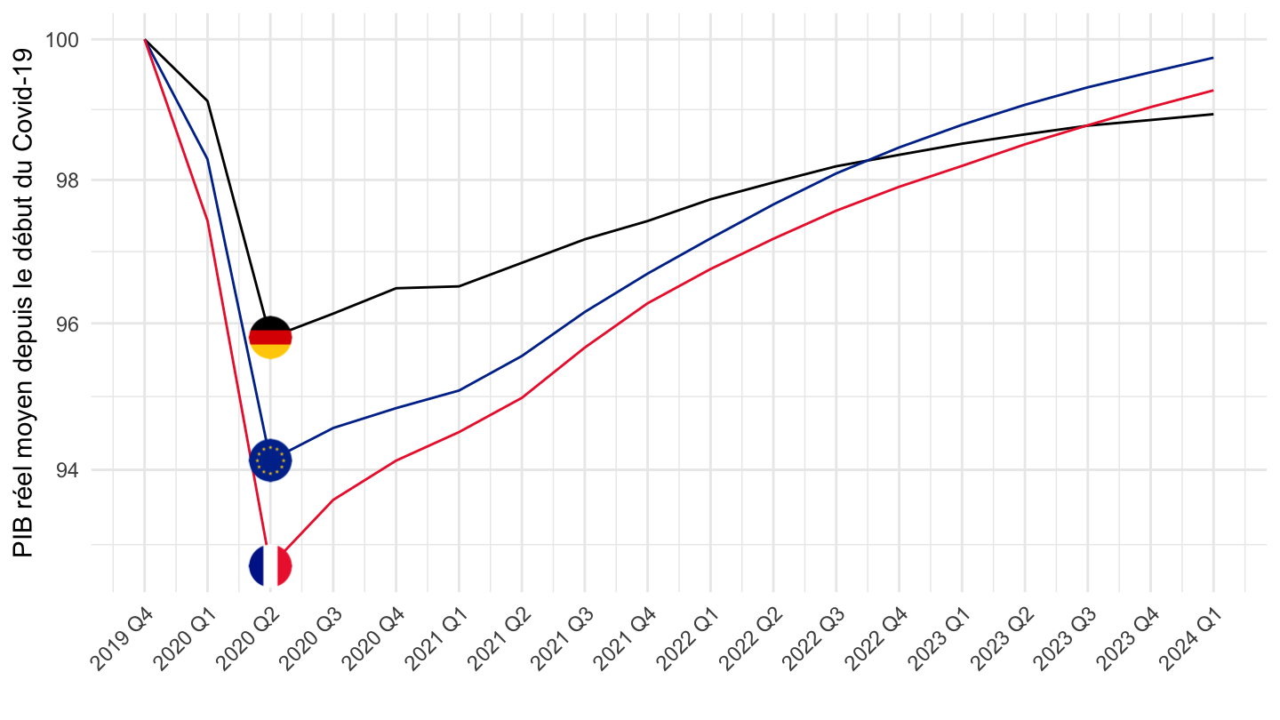
Average 2
Code
namq_10_gdp %>%
  filter(na_item == "B1GQ",
         # SCA: Seasonally and calendar adjusted data
         s_adj == "SCA",
         # CLV10_MEUR: Chain linked volumes (2010), million euro
         unit == "CLV10_MEUR",
         geo %in% c("DE", "EA", "FR", "EL", "BE", "CH", "IT", "ES")) %>%
  quarter_to_date %>%
  filter(date >= as.Date("2019-10-01")) %>%
  group_by(geo) %>%
  arrange(date) %>%
  mutate(values = 100*values/values[date == as.Date("2019-10-01")],
         values = cumsum(values) / seq_along(values)) %>%

  mutate(Geo = ifelse(geo == "EA", "Europe", Geo)) %>%
  left_join(colors, by = c("Geo" = "country")) %>%
  mutate(date = zoo::as.yearqtr(paste0(year(date), " Q", quarter(date)))) %>%
  ggplot + geom_line(aes(x = date, y = values, color = color)) + add_8flags +
  scale_color_identity() + theme_minimal() + xlab("") + ylab("PIB réel moyen depuis le début du Covid-19") +
  zoo::scale_x_yearqtr(labels = date_format("%Y Q%q"),
                       breaks = seq(zoo::as.yearqtr("2019 Q4"), zoo::as.yearqtr("2100 Q1"), by = 0.25)) +
  theme(legend.position = c(0.35, 0.85),
        legend.title = element_blank(),
        axis.text.x = element_text(angle = 45, vjust = 1, hjust = 1)) +
  scale_y_log10(breaks = seq(10, 300, 2))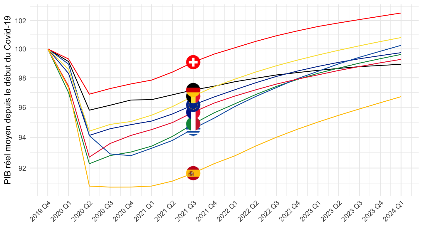
Deflators
Shall we compare deflators to inflation ? (do a stacked graph with both)
GDP
Table, PD_PCH_SM_EUR
Code
namq_10_gdp %>%
  filter(na_item == "B1GQ",
         s_adj == "NSA",
         unit == "PD_PCH_SM_EUR",
         time %in% c("2022Q1", "2022Q2", "2022Q3","2022Q4",  max(time))) %>%
  select(time, na_item, geo, Geo, values) %>%

  spread(time, values) %>%
  arrange(-`2022Q4`) %>%
  {if (is_html_output()) datatable(., filter = 'top', rownames = F) else .}
Table, PD15_EUR
Code
namq_10_gdp %>%
  filter(na_item == "B1GQ",
         s_adj == "NSA",
         unit == "PD15_EUR",
         time %in% c("2022Q1", "2022Q2", "2022Q3","2022Q4",  max(time))) %>%
  select(time, na_item, geo, Geo, values) %>%

  spread(time, values) %>%
  arrange(-`2022Q4`) %>%
  {if (is_html_output()) datatable(., filter = 'top', rownames = F) else .}
Germany, France
GDP
All
Code
namq_10_gdp %>%
  filter(na_item == "B1GQ",
         s_adj == "NSA",
         unit == "PD15_EUR",
         geo %in% c("FR", "DE")) %>%
  quarter_to_date %>%
  filter(date >= as.Date("1996-01-01")) %>%

  mutate(Geo= ifelse(geo == "EA", "Europe", Geo)) %>%
  left_join(colors, by = c("Geo" = "country")) %>%
  group_by(Geo) %>%
  mutate(values = 100*values/values[1]) %>%
  ggplot + geom_line(aes(x = date, y = values, color = color)) +
  scale_color_identity() + theme_minimal()  + add_2flags +
  scale_x_date(breaks = as.Date(paste0(seq(1960, 2100, 2), "-01-01")),
               labels = date_format("%Y")) +
  theme(legend.position = "none",
        legend.title = element_blank()) +
  xlab("") + ylab("GDP Deflator") +
  scale_y_log10(breaks = seq(90, 200, 5)) +
  geom_label_repel(data = . %>% filter(date == max(date)),
                   aes(x = date, y = values, label = round(values, 1), color = color))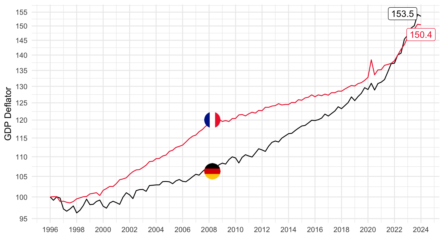
1999-
Code
namq_10_gdp %>%
  filter(na_item == "B1GQ",
         s_adj == "NSA",
         unit == "PD15_EUR",
         geo %in% c("FR", "DE")) %>%
  quarter_to_date %>%
  filter(date >= as.Date("1999-01-01")) %>%

  mutate(Geo= ifelse(geo == "EA", "Europe", Geo)) %>%
  left_join(colors, by = c("Geo" = "country")) %>%
  group_by(Geo) %>%
  mutate(values = 100*values/values[date == as.Date("1999-01-01")]) %>%
  ggplot + geom_line(aes(x = date, y = values, color = color)) +
  scale_color_identity() + theme_minimal()  + add_2flags +
  scale_x_date(breaks = as.Date(paste0(seq(1960, 2100, 2), "-01-01")),
               labels = date_format("%Y")) +
  theme(legend.position = "none",
        legend.title = element_blank()) +
  xlab("") + ylab("GDP Deflator") +
  scale_y_log10(breaks = seq(90, 200, 5)) +
  geom_label_repel(data = . %>% filter(date == max(date)),
                   aes(x = date, y = values, label = round(values, 1), color = color))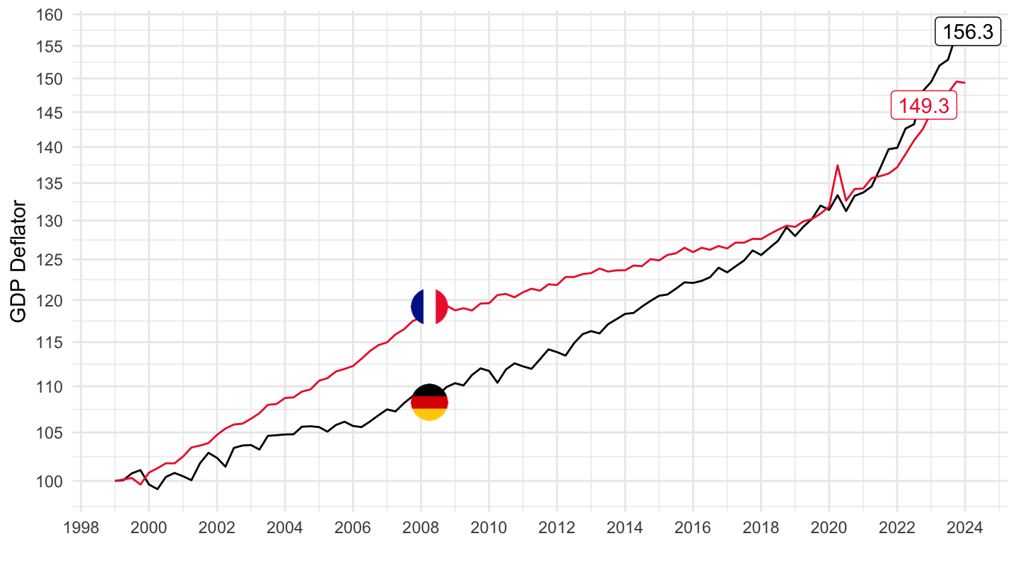
2018-
Code
namq_10_gdp %>%
  filter(na_item == "B1GQ",
         s_adj == "NSA",
         unit == "PD15_EUR",
         geo %in% c("FR", "DE")) %>%
  quarter_to_date %>%
  filter(date >= as.Date("2018-01-01")) %>%

  mutate(Geo= ifelse(geo == "EA", "Europe", Geo)) %>%
  left_join(colors, by = c("Geo" = "country")) %>%
  group_by(Geo) %>%
  mutate(values = 100*values/values[date == as.Date("2018-01-01")]) %>%
  ggplot + geom_line(aes(x = date, y = values, color = color)) +
  scale_color_identity() + theme_minimal()  + add_2flags +
  scale_x_date(breaks = as.Date(paste0(seq(1960, 2100, 1), "-01-01")),
               labels = date_format("%Y")) +
  theme(legend.position = "none",
        legend.title = element_blank()) +
  xlab("") + ylab("GDP Deflator") +
  scale_y_log10(breaks = seq(90, 200, 5)) +
  geom_label(data = . %>% filter(date == max(date)),
                   aes(x = date, y = values, label = round(values, 1), color = color))
Consumption
All
Code
namq_10_gdp %>%
  filter(na_item == "P3",
         s_adj == "NSA",
         unit == "PD15_EUR",
         geo %in% c("FR", "DE")) %>%
  quarter_to_date %>%
  filter(date >= as.Date("1996-01-01")) %>%

  mutate(Geo= ifelse(geo == "EA", "Europe", Geo)) %>%
  left_join(colors, by = c("Geo" = "country")) %>%
  group_by(Geo) %>%
  mutate(values = 100*values/values[1]) %>%
  ggplot + geom_line(aes(x = date, y = values, color = color)) +
  scale_color_identity() + theme_minimal()  + add_2flags +
  scale_x_date(breaks = as.Date(paste0(seq(1960, 2100, 2), "-01-01")),
               labels = date_format("%Y")) +
  theme(legend.position = "none",
        legend.title = element_blank()) +
  xlab("") + ylab("Consumption Deflator") +
  scale_y_log10(breaks = seq(90, 200, 5)) +
  geom_label_repel(data = . %>% filter(date == max(date)),
                   aes(x = date, y = values, label = round(values, 1), color = color))
1999-
Code
namq_10_gdp %>%
  filter(na_item == "P3",
         s_adj == "NSA",
         unit == "PD15_EUR",
         geo %in% c("FR", "DE")) %>%
  quarter_to_date %>%
  filter(date >= as.Date("1999-01-01")) %>%

  mutate(Geo= ifelse(geo == "EA", "Europe", Geo)) %>%
  left_join(colors, by = c("Geo" = "country")) %>%
  group_by(Geo) %>%
  mutate(values = 100*values/values[date == as.Date("1999-01-01")]) %>%
  ggplot + geom_line(aes(x = date, y = values, color = color)) +
  scale_color_identity() + theme_minimal()  + add_2flags +
  scale_x_date(breaks = as.Date(paste0(seq(1960, 2100, 2), "-01-01")),
               labels = date_format("%Y")) +
  theme(legend.position = "none",
        legend.title = element_blank()) +
  xlab("") + ylab("Consumption Deflator") +
  scale_y_log10(breaks = seq(90, 200, 5)) +
  geom_label_repel(data = . %>% filter(date == max(date)),
                   aes(x = date, y = values, label = round(values, 1), color = color))
GDP, Consumption
Code
namq_10_gdp %>%
  filter(na_item %in% c("P3", "B1GQ"),
         s_adj == "NSA",
         unit == "PD15_EUR",
         geo %in% c("FR", "DE")) %>%
  quarter_to_date %>%
  filter(date >= as.Date("1996-01-01")) %>%


  mutate(Geo= ifelse(geo == "EA", "Europe", Geo)) %>%
  left_join(colors, by = c("Geo" = "country")) %>%
  group_by(Geo) %>%
  mutate(values = 100*values/values[1]) %>%
  ggplot + geom_line(aes(x = date, y = values, color = color, linetype = Na_item)) +
  scale_color_identity() + theme_minimal()  + add_4flags +
  scale_x_date(breaks = as.Date(paste0(seq(1960, 2100, 2), "-01-01")),
               labels = date_format("%Y")) +
  theme(legend.position = "none",
        legend.title = element_blank()) +
  xlab("") + ylab("GDP, Consumption Deflator") +
  scale_y_log10(breaks = seq(90, 200, 5)) +
  geom_label_repel(data = . %>% filter(date == max(date)),
                   aes(x = date, y = values, label = round(values, 1), color = color, linetype = Na_item))
Greece, Portugal, France, Germany
2021-
Code
namq_10_gdp %>%
  filter(na_item == "B1GQ",
         s_adj == "NSA",
         unit == "PD15_EUR",
         geo %in% c("FR", "DE", "EL", "PT")) %>%
  quarter_to_date %>%
  filter(date >= as.Date("2021-01-01")) %>%

  mutate(Geo= ifelse(geo == "EA", "Europe", Geo)) %>%
  left_join(colors, by = c("Geo" = "country")) %>%
  group_by(Geo) %>%
  mutate(values = 100*values/values[date == as.Date("2021-01-01")]) %>%
  ggplot + geom_line(aes(x = date, y = values, color = color)) +
  scale_color_identity() + theme_minimal()  + add_4flags +
  scale_x_date(breaks = as.Date(paste0(seq(1960, 2100, 1), "-01-01")),
               labels = date_format("%Y")) +
  theme(legend.position = "none",
        legend.title = element_blank()) +
  xlab("") + ylab("GDP Deflator") +
  scale_y_log10(breaks = seq(90, 200, 2)) +
  geom_label_repel(data = . %>% filter(date == max(date)),
                   aes(x = date, y = values, label = round(values, 1), color = color))
Germany, France, Euro Area, Italy, Spain
PD_PCH_SM_EUR
1996-
Code
namq_10_gdp %>%
  filter(na_item == "B1GQ",
         s_adj == "NSA",
         unit == "PD_PCH_SM_EUR",
         geo %in% c("FR", "DE", "EA", "IT")) %>%
  transmute(time, na_item, geo, Geo, values = values/100) %>%
  quarter_to_date %>%
  filter(date >= as.Date("1996-01-01")) %>%

  mutate(Geo= ifelse(geo == "EA", "Europe", Geo)) %>%
  left_join(colors, by = c("Geo" = "country")) %>%
  ggplot + geom_line(aes(x = date, y = values, color = color)) +
  scale_color_identity() + theme_minimal()  + add_4flags +
  scale_x_date(breaks = as.Date(paste0(seq(1960, 2100, 2), "-01-01")),
               labels = date_format("%Y")) +
  theme(legend.position = "none",
        legend.title = element_blank()) +
  xlab("") + ylab("Net Exports (% of GDP)") +
  scale_y_continuous(breaks = 0.01*seq(-30, 30, 1),
                labels = percent_format(a = 1)) +
  geom_hline(yintercept = 0, linetype = "dashed",  color = "black")
2010-
Code
namq_10_gdp %>%
  filter(na_item == "B1GQ",
         s_adj == "NSA",
         unit == "PD_PCH_SM_EUR",
         geo %in% c("FR", "DE", "EA", "IT")) %>%
  transmute(time, na_item, geo, Geo, values = values/100) %>%
  quarter_to_date %>%
  filter(date >= as.Date("2010-01-01")) %>%

  mutate(Geo= ifelse(geo == "EA", "Europe", Geo)) %>%
  left_join(colors, by = c("Geo" = "country")) %>%
  ggplot + geom_line(aes(x = date, y = values, color = color)) +
  scale_color_identity() + theme_minimal()  + add_4flags +
  scale_x_date(breaks = as.Date(paste0(seq(1960, 2100, 2), "-01-01")),
               labels = date_format("%Y")) +
  theme(legend.position = "none",
        legend.title = element_blank()) +
  xlab("") + ylab("GDP Deflator, Annual % change") +
  scale_y_continuous(breaks = 0.01*seq(-30, 30, 1),
                labels = percent_format(a = 1)) +
  geom_hline(yintercept = 0, linetype = "dashed",  color = "black")
2018-
GDP
Code
namq_10_gdp %>%
  filter(na_item == "B1GQ",
         s_adj == "NSA",
         unit == "PD_PCH_SM_EUR",
         geo %in% c("FR", "DE", "EA", "IT", "ES")) %>%
  transmute(time, na_item, geo, Geo, values = values/100) %>%
  quarter_to_date %>%
  filter(date >= as.Date("2018-01-01")) %>%

  mutate(Geo= ifelse(geo == "EA", "Europe", Geo)) %>%
  left_join(colors, by = c("Geo" = "country")) %>%
  ggplot + geom_line(aes(x = date, y = values, color = color)) +
  scale_color_identity() + theme_minimal()  + add_5flags +
  scale_x_date(breaks = as.Date(paste0(seq(1960, 2100, 1), "-01-01")),
               labels = date_format("%Y")) +
  theme(legend.position = "none",
        legend.title = element_blank()) +
  xlab("") + ylab("GDP Deflator, Annual % change") +
  scale_y_continuous(breaks = 0.01*seq(-30, 30, 1),
                labels = percent_format(a = 1)) +
  geom_hline(yintercept = 0, linetype = "dashed",  color = "black")
P3 Consumption Deflator
Code
namq_10_gdp %>%
  filter(na_item == "P3",
         s_adj == "NSA",
         unit == "PD_PCH_SM_EUR",
         geo %in% c("FR", "DE", "EA", "IT", "ES")) %>%
  transmute(time, na_item, geo, Geo, values = values/100) %>%
  quarter_to_date %>%
  filter(date >= as.Date("2018-01-01")) %>%

  mutate(Geo= ifelse(geo == "EA", "Europe", Geo)) %>%
  left_join(colors, by = c("Geo" = "country")) %>%
  ggplot + geom_line(aes(x = date, y = values, color = color)) +
  scale_color_identity() + theme_minimal()  + add_5flags +
  scale_x_date(breaks = as.Date(paste0(seq(1960, 2100, 1), "-01-01")),
               labels = date_format("%Y")) +
  theme(legend.position = "none",
        legend.title = element_blank()) +
  xlab("") + ylab("Consumption Deflator, Annual % change") +
  scale_y_continuous(breaks = 0.01*seq(-30, 30, 1),
                labels = percent_format(a = 1)) +
  geom_hline(yintercept = 0, linetype = "dashed",  color = "black")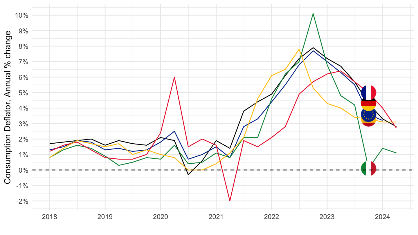
P31_S14 Final consumption expenditure of households
Code
namq_10_gdp %>%
  filter(na_item == "P31_S14",
         s_adj == "NSA",
         unit == "PD_PCH_SM_EUR",
         geo %in% c("FR", "DE", "EA", "IT", "ES")) %>%
  transmute(time, na_item, geo, Geo, values = values/100) %>%
  quarter_to_date %>%
  filter(date >= as.Date("2018-01-01")) %>%

  mutate(Geo= ifelse(geo == "EA", "Europe", Geo)) %>%
  left_join(colors, by = c("Geo" = "country")) %>%
  ggplot + geom_line(aes(x = date, y = values, color = color)) +
  scale_color_identity() + theme_minimal()  + add_4flags +
  scale_x_date(breaks = as.Date(paste0(seq(1960, 2100, 1), "-01-01")),
               labels = date_format("%Y")) +
  theme(legend.position = "none",
        legend.title = element_blank()) +
  xlab("") + ylab("Final consumption expenditure of households, Annual % change") +
  scale_y_continuous(breaks = 0.01*seq(-30, 30, 1),
                labels = percent_format(a = 1)) +
  geom_hline(yintercept = 0, linetype = "dashed",  color = "black")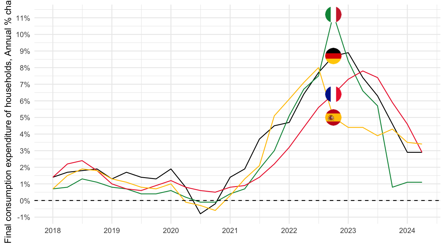
P41 Actual Individual Consumption
Code
namq_10_gdp %>%
  filter(na_item == "P41",
         s_adj == "NSA",
         unit == "PD_PCH_SM_EUR",
         geo %in% c("FR", "DE", "EA", "IT", "ES")) %>%
  transmute(time, na_item, geo, Geo, values = values/100) %>%
  quarter_to_date %>%
  filter(date >= as.Date("2018-01-01")) %>%

  mutate(Geo= ifelse(geo == "EA", "Europe", Geo)) %>%
  left_join(colors, by = c("Geo" = "country")) %>%
  ggplot + geom_line(aes(x = date, y = values, color = color)) +
  scale_color_identity() + theme_minimal()  + add_4flags +
  scale_x_date(breaks = as.Date(paste0(seq(1960, 2100, 1), "-01-01")),
               labels = date_format("%Y")) +
  theme(legend.position = "none",
        legend.title = element_blank()) +
  xlab("") + ylab("Actual Individual Consumption, Annual % change") +
  scale_y_continuous(breaks = 0.01*seq(-30, 30, 1),
                labels = percent_format(a = 1)) +
  geom_hline(yintercept = 0, linetype = "dashed",  color = "black")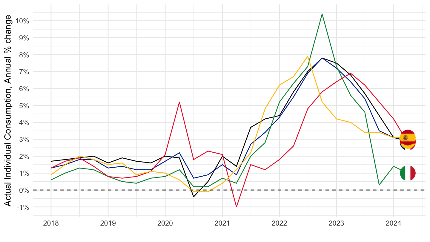
Net Exports of Goods
Table
Code
namq_10_gdp %>%
  filter(na_item %in% c("P61", "P71"),
         s_adj == "NSA",
         unit == "PC_GDP",
         time %in% c("1989Q4", "1999Q4", "2009Q4", "2019Q4", "2022Q2", "2022Q3")) %>%
  select(time, na_item, geo, Geo, values) %>%
  mutate(values = round(values, 1)) %>%

  spread(na_item, values) %>%
  mutate(NX = round(P61 - P71, 1)) %>%
  select(-P61, -P71) %>%
  spread(time, NX) %>%
  arrange(`2022Q3`) %>%
  {if (is_html_output()) datatable(., filter = 'top', rownames = F) else .}
Germany, France, Netherlands
1995-
Code
namq_10_gdp %>%
  filter(na_item %in% c("P61", "P71"),
         s_adj == "SCA",
         unit == "PC_GDP",
         geo %in% c("FR", "DE", "NL")) %>%
  select(time, na_item, geo, Geo, values) %>%
  quarter_to_date %>%
  filter(date >= as.Date("1995-01-01")) %>%

  mutate(Geo= ifelse(geo == "EA", "Europe", Geo)) %>%
  spread(na_item, values) %>%
  mutate(values = (P61 - P71)/100) %>%
  left_join(colors, by = c("Geo" = "country")) %>%
  mutate(color = ifelse(geo == "NL", color2, color)) %>%
  ggplot + geom_line(aes(x = date, y = values, color = color)) +
  scale_color_identity() + theme_minimal()  +
  scale_x_date(breaks = as.Date(paste0(seq(1960, 2100, 5), "-01-01")),
               labels = date_format("%Y")) +
  add_3flags +
  theme(legend.position = "none",
        legend.title = element_blank()) +
  xlab("") + ylab("Net Exports (% of GDP)") +
  scale_y_continuous(breaks = 0.01*seq(-30, 30, 1),
                labels = percent_format(a = 1)) +
  geom_hline(yintercept = 0, linetype = "dashed",  color = "black")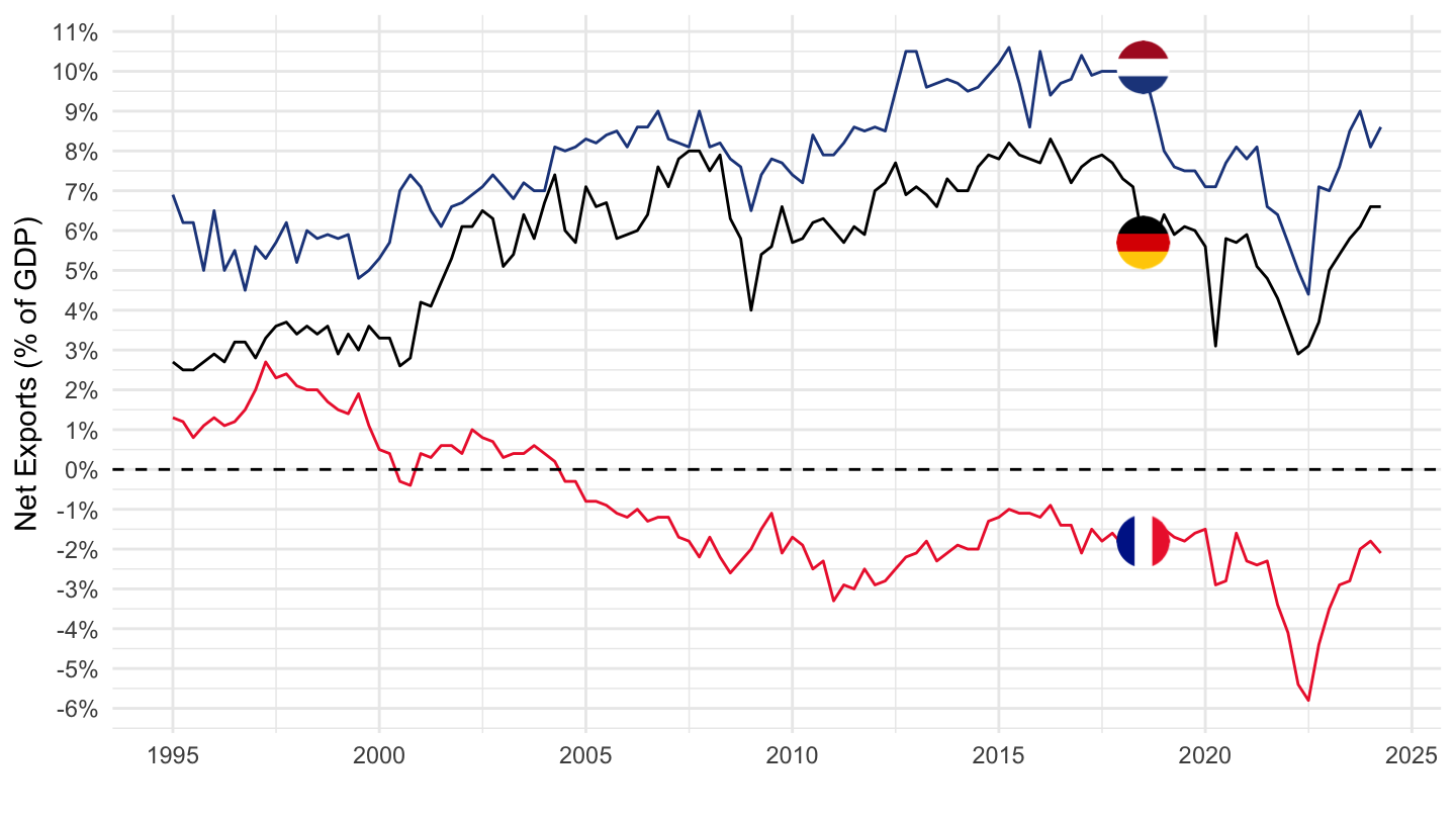
Germany, France, Eurozone, Italy
All
Code
namq_10_gdp %>%
  filter(na_item %in% c("P61", "P71"),
         s_adj == "NSA",
         unit == "PC_GDP",
         geo %in% c("FR", "DE", "EA", "IT")) %>%
  select(time, na_item, geo, Geo, values) %>%
  quarter_to_date %>%

  mutate(Geo= ifelse(geo == "EA", "Europe", Geo)) %>%
  spread(na_item, values) %>%
  mutate(values = (P61 - P71)/100) %>%
  left_join(colors, by = c("Geo" = "country")) %>%
  ggplot + geom_line(aes(x = date, y = values, color = color)) +
  scale_color_identity() + theme_minimal()  + add_4flags +
  scale_x_date(breaks = as.Date(paste0(seq(1960, 2100, 2), "-01-01")),
               labels = date_format("%Y")) +
  theme(legend.position = "none",
        legend.title = element_blank()) +
  xlab("") + ylab("Net Exports (% of GDP)") +
  scale_y_continuous(breaks = 0.01*seq(-30, 30, 1),
                labels = percent_format(a = 1)) +
  geom_hline(yintercept = 0, linetype = "dashed",  color = "black")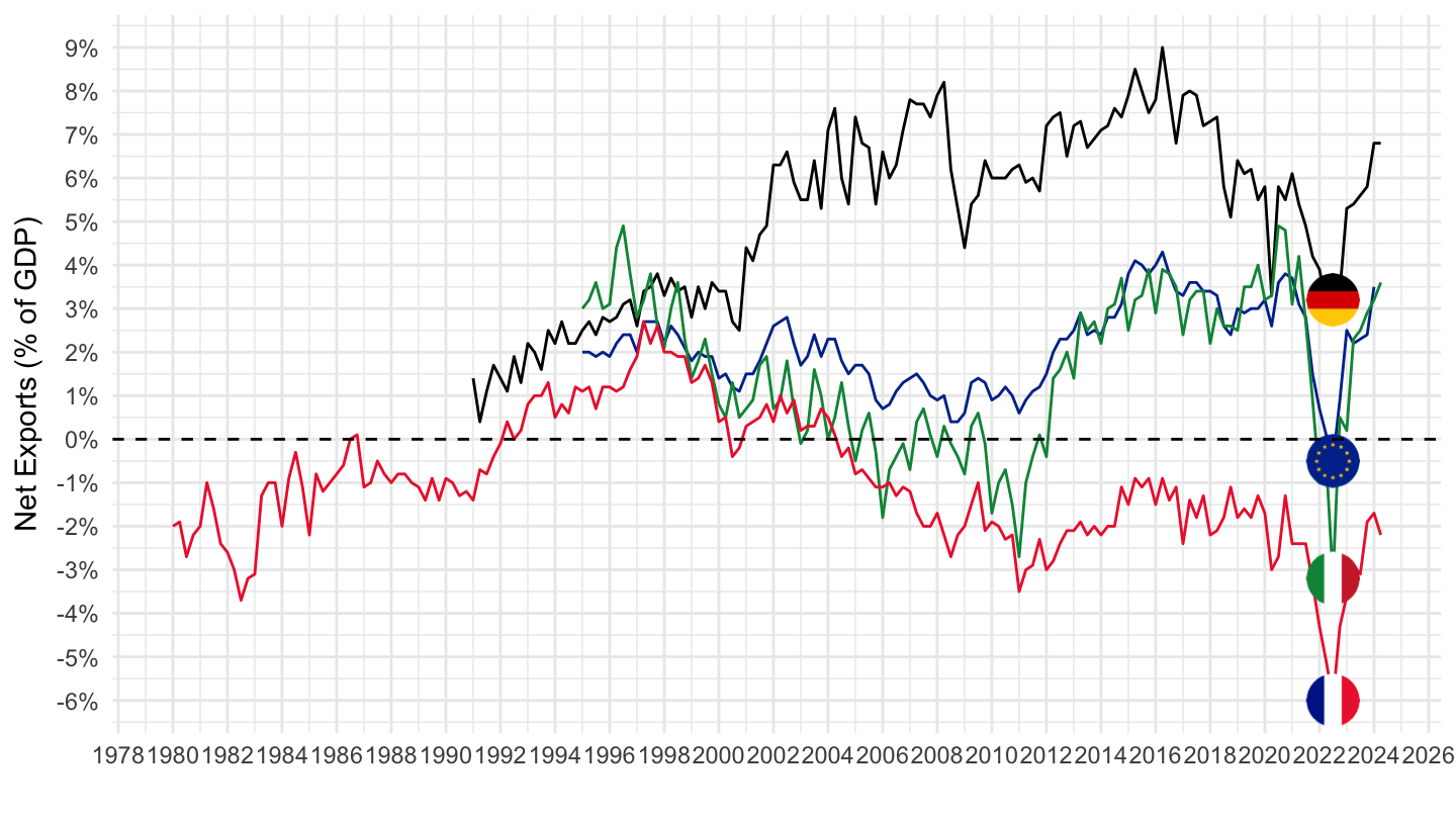
1990-
Code
namq_10_gdp %>%
  filter(na_item %in% c("P61", "P71"),
         s_adj == "NSA",
         unit == "PC_GDP",
         geo %in% c("FR", "DE", "EA", "IT")) %>%
  select(time, na_item, geo, Geo, values) %>%
  quarter_to_date %>%
  filter(date >= as.Date("1990-01-01")) %>%

  mutate(Geo= ifelse(geo == "EA", "Europe", Geo)) %>%
  spread(na_item, values) %>%
  mutate(values = (P61 - P71)/100) %>%
  left_join(colors, by = c("Geo" = "country")) %>%
  ggplot + geom_line(aes(x = date, y = values, color = color)) +
  scale_color_identity() + theme_minimal()  + add_4flags +
  scale_x_date(breaks = as.Date(paste0(seq(1960, 2100, 2), "-01-01")),
               labels = date_format("%Y")) +
  theme(legend.position = "none",
        legend.title = element_blank()) +
  xlab("") + ylab("Net Exports (% of GDP)") +
  scale_y_continuous(breaks = 0.01*seq(-30, 30, 1),
                labels = percent_format(a = 1)) +
  geom_hline(yintercept = 0, linetype = "dashed",  color = "black")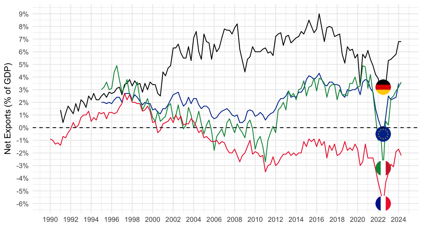
1995-
English
Code
namq_10_gdp %>%
  filter(na_item %in% c("P61", "P71"),
         s_adj == "SCA",
         unit == "PC_GDP",
         geo %in% c("FR", "DE", "EA", "IT")) %>%
  select(time, na_item, geo, Geo, values) %>%
  quarter_to_date %>%
  filter(date >= as.Date("1995-01-01")) %>%

  mutate(Geo= ifelse(geo == "EA", "Europe", Geo)) %>%
  spread(na_item, values) %>%
  mutate(values = (P61 - P71)/100) %>%
  left_join(colors, by = c("Geo" = "country")) %>%
  ggplot + geom_line(aes(x = date, y = values, color = color)) +
  scale_color_identity() + theme_minimal()  + add_4flags +
  scale_x_date(breaks = as.Date(paste0(seq(1960, 2100, 2), "-01-01")),
               labels = date_format("%Y")) +
  theme(legend.position = "none",
        legend.title = element_blank()) +
  xlab("") + ylab("Net Exports (% of GDP)") +
  scale_y_continuous(breaks = 0.01*seq(-30, 30, 1),
                labels = percent_format(a = 1)) +
  geom_hline(yintercept = 0, linetype = "dashed",  color = "black")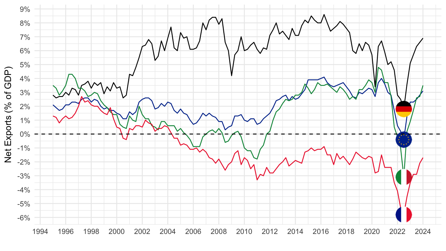
Français
Code
namq_10_gdp %>%
  filter(na_item %in% c("P61", "P71"),
         s_adj == "SCA",
         unit == "PC_GDP",
         geo %in% c("FR", "DE", "EA", "IT")) %>%
  select(time, na_item, geo, Geo, values) %>%
  quarter_to_date %>%
  filter(date >= as.Date("1995-01-01")) %>%

  mutate(Geo= ifelse(geo == "EA", "Europe", Geo)) %>%
  spread(na_item, values) %>%
  mutate(values = (P61 - P71)/100) %>%
  left_join(colors, by = c("Geo" = "country")) %>%
  ggplot + geom_line(aes(x = date, y = values, color = color)) +
  scale_color_identity() + theme_minimal()  + add_4flags +
  scale_x_date(breaks = as.Date(paste0(seq(1960, 2100, 2), "-01-01")),
               labels = date_format("%Y")) +
  theme(legend.position = "none",
        legend.title = element_blank()) +
  xlab("") + ylab("Balance commerciale (% du PIB)") +
  scale_y_continuous(breaks = 0.01*seq(-30, 30, 1),
                labels = percent_format(a = 1)) +
  geom_hline(yintercept = 0, linetype = "dashed",  color = "black")
1996-
Code
namq_10_gdp %>%
  filter(na_item %in% c("P61", "P71"),
         s_adj == "NSA",
         unit == "PC_GDP",
         geo %in% c("FR", "DE", "EA", "IT")) %>%
  select(time, na_item, geo, Geo, values) %>%
  quarter_to_date %>%
  filter(date >= as.Date("1996-01-01")) %>%

  mutate(Geo= ifelse(geo == "EA", "Europe", Geo)) %>%
  spread(na_item, values) %>%
  mutate(values = (P61 - P71)/100) %>%
  left_join(colors, by = c("Geo" = "country")) %>%
  ggplot + geom_line(aes(x = date, y = values, color = color)) +
  scale_color_identity() + theme_minimal()  + add_4flags +
  scale_x_date(breaks = as.Date(paste0(seq(1960, 2100, 2), "-01-01")),
               labels = date_format("%Y")) +
  theme(legend.position = "none",
        legend.title = element_blank()) +
  xlab("") + ylab("Net Exports (% of GDP)") +
  scale_y_continuous(breaks = 0.01*seq(-30, 30, 1),
                labels = percent_format(a = 1)) +
  geom_hline(yintercept = 0, linetype = "dashed",  color = "black")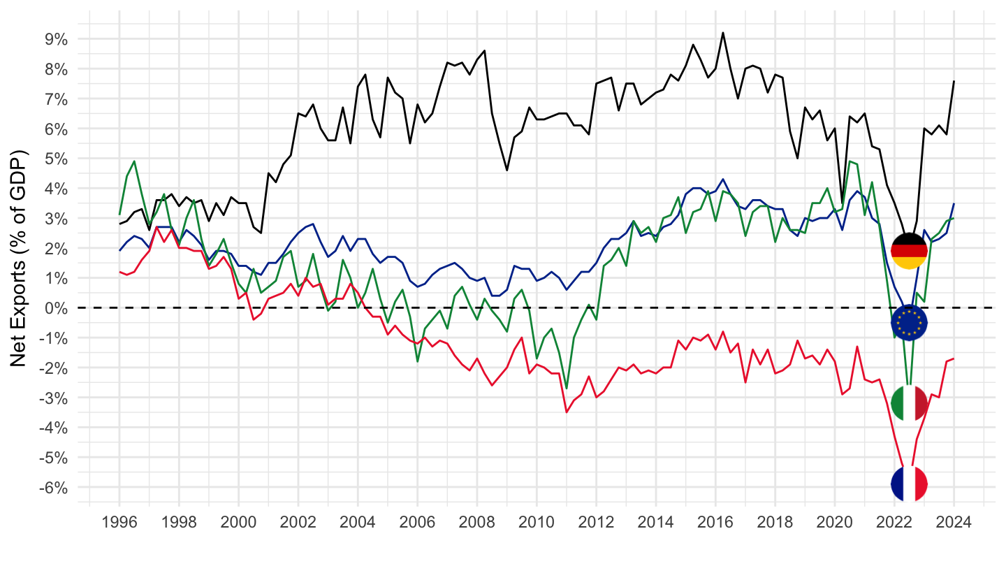
France vs. Gemrany
Français
Code
namq_10_gdp %>%
  filter(na_item %in% c("P61", "P71"),
         s_adj == "SCA",
         unit == "PC_GDP",
         geo %in% c("FR", "DE", "EA19")) %>%
  select(time, na_item, geo, Geo, values) %>%
  quarter_to_date %>%
  filter(date >= as.Date("1995-01-01")) %>%

  mutate(Geo= ifelse(geo == "EA19", "Europe", Geo)) %>%
  spread(na_item, values) %>%
  mutate(values = (P61 - P71)/100) %>%
  left_join(colors, by = c("Geo" = "country")) %>%
  ggplot + geom_line(aes(x = date, y = values, color = color)) +
  scale_color_identity() + theme_minimal()  + add_3flags +
  scale_x_date(breaks = as.Date(paste0(seq(1960, 2100, 2), "-01-01")),
               labels = date_format("%Y")) +
  theme(legend.position = "none",
        legend.title = element_blank()) +
  xlab("") + ylab("Balance commerciale (% du PIB)") +
  scale_y_continuous(breaks = 0.01*seq(-30, 30, 1),
                labels = percent_format(a = 1)) +
  geom_hline(yintercept = 0, linetype = "dashed",  color = "black")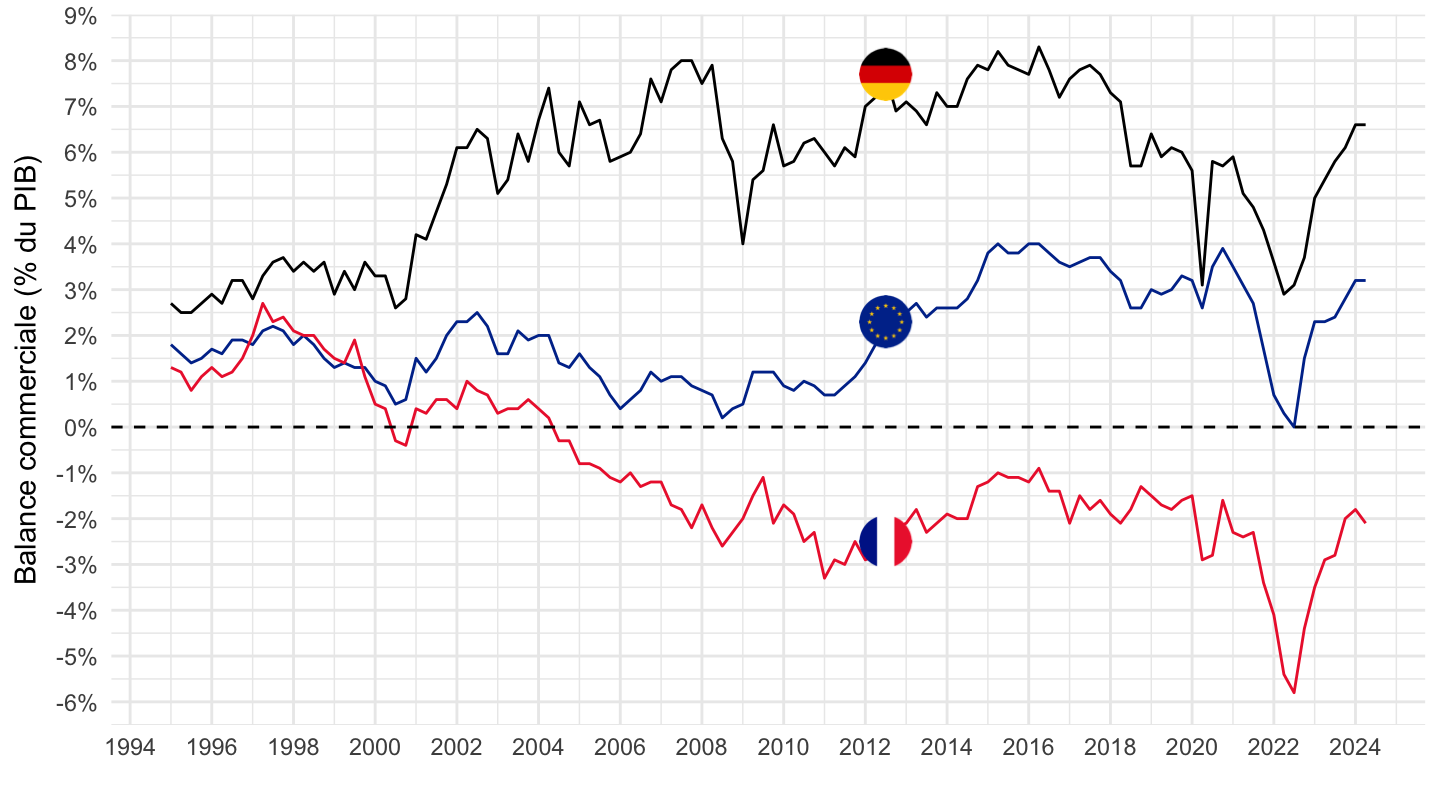
Government Spending
Final consumption expenditure of general government
Code
namq_10_gdp %>%
  filter(na_item %in% c("P3_S13"),
         s_adj == "SCA",
         unit == "PC_GDP",
         geo %in% c("FR", "DE", "NL", "IT", "ES")) %>%
  quarter_to_date %>%
  filter(date >= as.Date("1995-01-01")) %>%

  mutate(Geo= ifelse(geo == "EA", "Europe", Geo)) %>%
  left_join(colors, by = c("Geo" = "country")) %>%
  mutate(color = ifelse(geo == "NL", color2, color)) %>%
  mutate(values = values/100) %>%
  ggplot + geom_line(aes(x = date, y = values, color = color)) +
  scale_color_identity() + theme_minimal()  +
  scale_x_date(breaks = as.Date(paste0(seq(1960, 2100, 2), "-01-01")),
               labels = date_format("%Y")) +
  add_5flags +
  theme(legend.position = "none",
        legend.title = element_blank()) +
  xlab("") + ylab("Government Consumption (% of GDP)") +
  scale_y_continuous(breaks = 0.01*seq(-30, 100, 1),
                labels = percent_format(a = 1))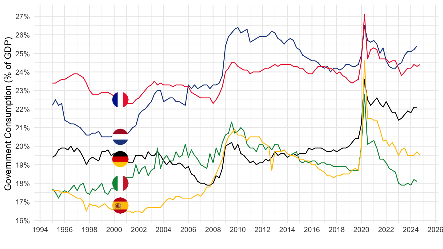
Individual consumption expenditure of general government
Code
namq_10_gdp %>%
  filter(na_item %in% c("P31_S13"),
         s_adj == "SCA",
         unit == "PC_GDP",
         geo %in% c("FR", "DE", "NL", "IT", "ES")) %>%
  quarter_to_date %>%
  filter(date >= as.Date("1995-01-01")) %>%

  mutate(Geo= ifelse(geo == "EA", "Europe", Geo)) %>%
  left_join(colors, by = c("Geo" = "country")) %>%
  mutate(color = ifelse(geo == "NL", color2, color)) %>%
  mutate(values = values/100) %>%
  ggplot + geom_line(aes(x = date, y = values, color = color)) +
  scale_color_identity() + theme_minimal()  +
  scale_x_date(breaks = as.Date(paste0(seq(1960, 2100, 2), "-01-01")),
               labels = date_format("%Y")) +
  add_5flags +
  theme(legend.position = "none",
        legend.title = element_blank()) +
  xlab("") + ylab("Government Consumption (% of GDP)") +
  scale_y_continuous(breaks = 0.01*seq(-30, 100, 1),
                labels = percent_format(a = 1))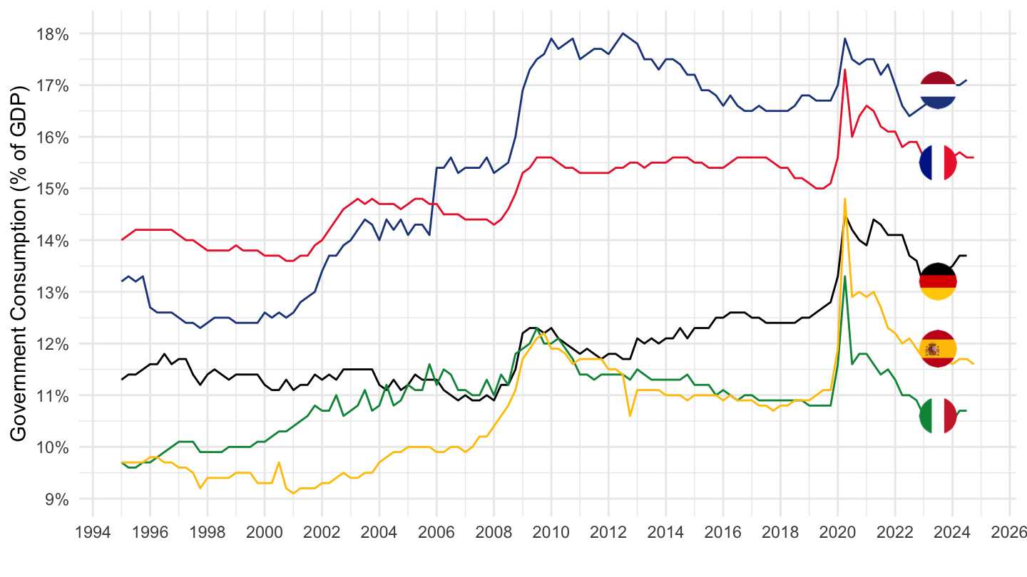
Collective consumption expenditure of general government
Code
namq_10_gdp %>%
  filter(na_item %in% c("P32_S13"),
         s_adj == "SCA",
         unit == "PC_GDP",
         geo %in% c("FR", "DE", "NL", "IT", "ES")) %>%
  quarter_to_date %>%
  filter(date >= as.Date("1995-01-01")) %>%

  mutate(Geo= ifelse(geo == "EA", "Europe", Geo)) %>%
  left_join(colors, by = c("Geo" = "country")) %>%
  mutate(color = ifelse(geo == "NL", color2, color)) %>%
  mutate(values = values/100) %>%
  ggplot + geom_line(aes(x = date, y = values, color = color)) +
  scale_color_identity() + theme_minimal()  +
  scale_x_date(breaks = as.Date(paste0(seq(1960, 2100, 2), "-01-01")),
               labels = date_format("%Y")) +
  add_5flags +
  theme(legend.position = "none",
        legend.title = element_blank()) +
  xlab("") + ylab("Government Consumption (% of GDP)") +
  scale_y_continuous(breaks = 0.01*seq(-30, 100, 1),
                labels = percent_format(a = 1))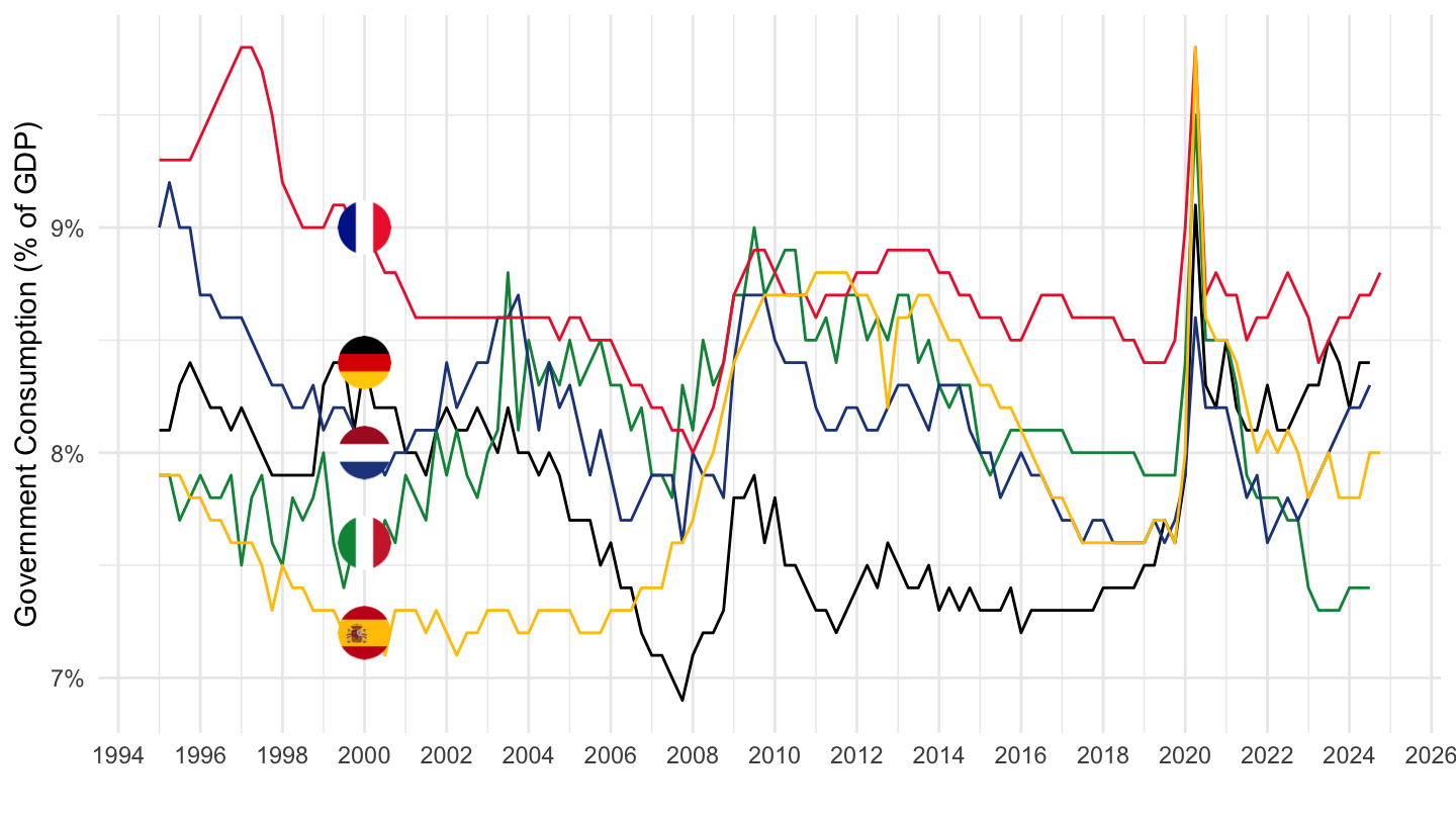
Net Exports
Table
Code
namq_10_gdp %>%
  filter(na_item %in% c("P6", "P7"),
         s_adj == "NSA",
         unit == "PC_GDP",
         time %in% c("1989Q4", "1999Q4", "2009Q4", "2019Q4", "2022Q2", "2022Q3")) %>%
  select(time, na_item, geo, Geo, values) %>%
  mutate(values = round(values, 1)) %>%

  spread(na_item, values) %>%
  mutate(NX = round(P6 - P7, 1)) %>%
  select(-P6, -P7) %>%
  spread(time, NX) %>%
  arrange(`2022Q3`) %>%
  {if (is_html_output()) datatable(., filter = 'top', rownames = F) else .}
Germany, France, Netherlands
1995-
Code
namq_10_gdp %>%
  filter(na_item %in% c("P6", "P7"),
         s_adj == "SCA",
         unit == "PC_GDP",
         geo %in% c("FR", "DE", "NL")) %>%
  select(time, na_item, geo, Geo, values) %>%
  quarter_to_date %>%
  filter(date >= as.Date("1995-01-01")) %>%

  mutate(Geo= ifelse(geo == "EA", "Europe", Geo)) %>%
  spread(na_item, values) %>%
  mutate(values = (P6 - P7)/100) %>%
  left_join(colors, by = c("Geo" = "country")) %>%
  mutate(color = ifelse(geo == "NL", color2, color)) %>%
  ggplot + geom_line(aes(x = date, y = values, color = color)) +
  scale_color_identity() + theme_minimal()  +
  scale_x_date(breaks = as.Date(paste0(seq(1960, 2100, 2), "-01-01")),
               labels = date_format("%Y")) +
  add_3flags +
  theme(legend.position = "none",
        legend.title = element_blank()) +
  xlab("") + ylab("Net Exports (% of GDP)") +
  scale_y_continuous(breaks = 0.01*seq(-30, 30, 1),
                labels = percent_format(a = 1)) +
  geom_hline(yintercept = 0, linetype = "dashed",  color = "black")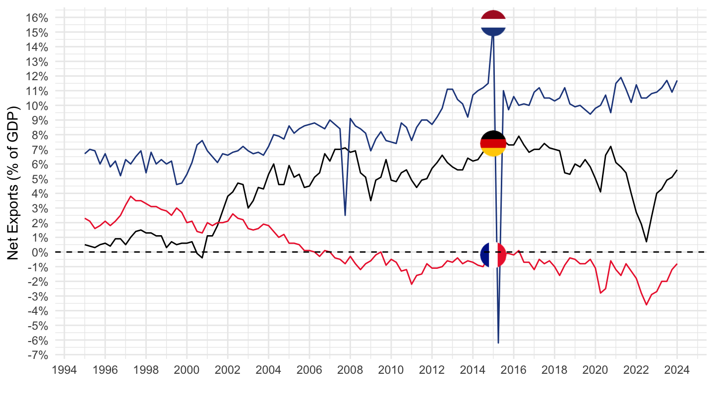
Germany, France, Eurozone, Italy
All
Code
namq_10_gdp %>%
  filter(na_item %in% c("P6", "P7"),
         s_adj == "NSA",
         unit == "PC_GDP",
         geo %in% c("FR", "DE", "EA", "IT")) %>%
  select(time, na_item, geo, Geo, values) %>%
  quarter_to_date %>%

  mutate(Geo= ifelse(geo == "EA", "Europe", Geo)) %>%
  spread(na_item, values) %>%
  mutate(values = (P6 - P7)/100) %>%
  left_join(colors, by = c("Geo" = "country")) %>%
  ggplot + geom_line(aes(x = date, y = values, color = color)) +
  scale_color_identity() + theme_minimal()  + add_4flags +
  scale_x_date(breaks = as.Date(paste0(seq(1960, 2100, 2), "-01-01")),
               labels = date_format("%Y")) +
  theme(legend.position = "none",
        legend.title = element_blank()) +
  xlab("") + ylab("Net Exports (% of GDP)") +
  scale_y_continuous(breaks = 0.01*seq(-30, 30, 1),
                labels = percent_format(a = 1)) +
  geom_hline(yintercept = 0, linetype = "dashed",  color = "black")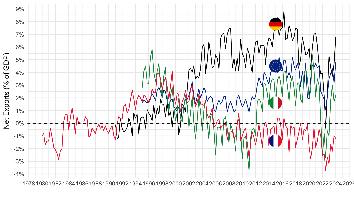
1990-
Code
namq_10_gdp %>%
  filter(na_item %in% c("P6", "P7"),
         s_adj == "NSA",
         unit == "PC_GDP",
         geo %in% c("FR", "DE", "EA", "IT")) %>%
  select(time, na_item, geo, Geo, values) %>%
  quarter_to_date %>%
  filter(date >= as.Date("1990-01-01")) %>%

  mutate(Geo= ifelse(geo == "EA", "Europe", Geo)) %>%
  spread(na_item, values) %>%
  mutate(values = (P6 - P7)/100) %>%
  left_join(colors, by = c("Geo" = "country")) %>%
  ggplot + geom_line(aes(x = date, y = values, color = color)) +
  scale_color_identity() + theme_minimal()  + add_4flags +
  scale_x_date(breaks = as.Date(paste0(seq(1960, 2100, 2), "-01-01")),
               labels = date_format("%Y")) +
  theme(legend.position = "none",
        legend.title = element_blank()) +
  xlab("") + ylab("Net Exports (% of GDP)") +
  scale_y_continuous(breaks = 0.01*seq(-30, 30, 1),
                labels = percent_format(a = 1)) +
  geom_hline(yintercept = 0, linetype = "dashed",  color = "black")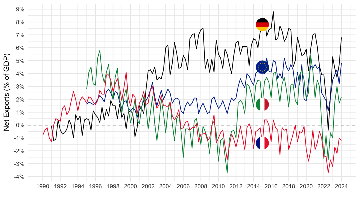
1995-
English
Code
namq_10_gdp %>%
  filter(na_item %in% c("P6", "P7"),
         s_adj == "SCA",
         unit == "PC_GDP",
         geo %in% c("FR", "DE", "EA", "IT")) %>%
  select(time, na_item, geo, Geo, values) %>%
  quarter_to_date %>%
  filter(date >= as.Date("1995-01-01")) %>%

  mutate(Geo= ifelse(geo == "EA", "Europe", Geo)) %>%
  spread(na_item, values) %>%
  mutate(values = (P6 - P7)/100) %>%
  left_join(colors, by = c("Geo" = "country")) %>%
  ggplot + geom_line(aes(x = date, y = values, color = color)) +
  scale_color_identity() + theme_minimal()  + add_4flags +
  scale_x_date(breaks = as.Date(paste0(seq(1960, 2100, 5), "-01-01")),
               labels = date_format("%Y")) +
  theme(legend.position = "none",
        legend.title = element_blank()) +
  xlab("") + ylab("Net Exports (% of GDP)") +
  scale_y_continuous(breaks = 0.01*seq(-30, 30, 1),
                labels = percent_format(a = 1)) +
  geom_hline(yintercept = 0, linetype = "dashed",  color = "black")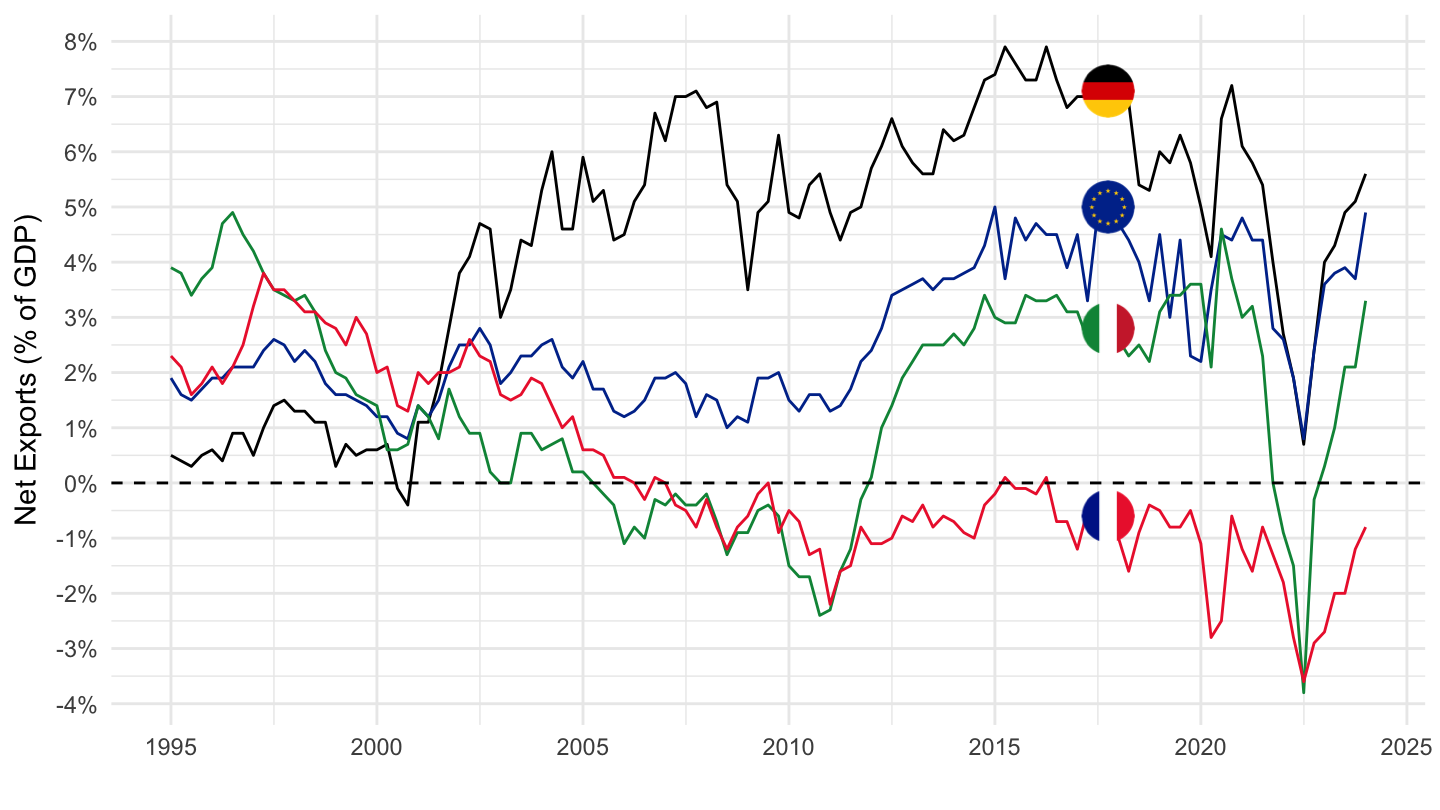
Français
Code
namq_10_gdp %>%
  filter(na_item %in% c("P6", "P7"),
         s_adj == "SCA",
         unit == "PC_GDP",
         geo %in% c("FR", "DE", "EA", "IT")) %>%
  select(time, na_item, geo, Geo, values) %>%
  quarter_to_date %>%
  filter(date >= as.Date("1995-01-01")) %>%

  mutate(Geo= ifelse(geo == "EA", "Europe", Geo)) %>%
  spread(na_item, values) %>%
  mutate(values = (P6 - P7)/100) %>%
  left_join(colors, by = c("Geo" = "country")) %>%
  ggplot + geom_line(aes(x = date, y = values, color = color)) +
  scale_color_identity() + theme_minimal()  + add_4flags +
  scale_x_date(breaks = as.Date(paste0(seq(1960, 2100, 5), "-01-01")),
               labels = date_format("%Y")) +
  theme(legend.position = "none",
        legend.title = element_blank()) +
  xlab("") + ylab("Balance commerciale (% du PIB)") +
  scale_y_continuous(breaks = 0.01*seq(-30, 30, 1),
                labels = percent_format(a = 1)) +
  geom_hline(yintercept = 0, linetype = "dashed",  color = "black")
1996-
Code
namq_10_gdp %>%
  filter(na_item %in% c("P6", "P7"),
         s_adj == "NSA",
         unit == "PC_GDP",
         geo %in% c("FR", "DE", "EA", "IT")) %>%
  select(time, na_item, geo, Geo, values) %>%
  quarter_to_date %>%
  filter(date >= as.Date("1996-01-01")) %>%

  mutate(Geo= ifelse(geo == "EA", "Europe", Geo)) %>%
  spread(na_item, values) %>%
  mutate(values = (P6 - P7)/100) %>%
  left_join(colors, by = c("Geo" = "country")) %>%
  ggplot + geom_line(aes(x = date, y = values, color = color)) +
  scale_color_identity() + theme_minimal()  + add_4flags +
  scale_x_date(breaks = as.Date(paste0(seq(1960, 2100, 2), "-01-01")),
               labels = date_format("%Y")) +
  theme(legend.position = "none",
        legend.title = element_blank()) +
  xlab("") + ylab("Net Exports (% of GDP)") +
  scale_y_continuous(breaks = 0.01*seq(-30, 30, 1),
                labels = percent_format(a = 1)) +
  geom_hline(yintercept = 0, linetype = "dashed",  color = "black")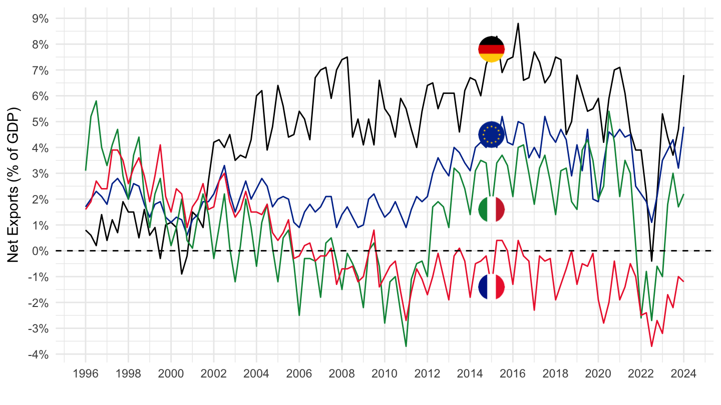
Germany, France, Eurozone, Belgium
Table
Code
namq_10_gdp %>%
  filter(na_item %in% c("P6", "P7"),
         s_adj == "SCA",
         unit == "PC_GDP",
         time == "2023Q1") %>%
  select(time, na_item, geo, Geo, values) %>%
  quarter_to_date %>%

  mutate(Geo= ifelse(geo == "EA", "Europe", Geo)) %>%
  spread(na_item, values) %>%
  mutate(values = (P6 - P7)) %>%
  arrange(values) %>%
  print_table_conditional
SCA
Code
namq_10_gdp %>%
  filter(na_item %in% c("P6", "P7"),
         s_adj == "SCA",
         unit == "PC_GDP",
         geo %in% c("FR", "DE", "EA", "BE")) %>%
  select(time, na_item, geo, Geo, values) %>%
  quarter_to_date %>%

  mutate(Geo= ifelse(geo == "EA", "Europe", Geo)) %>%
  spread(na_item, values) %>%
  mutate(values = (P6 - P7)/100) %>%
  left_join(colors, by = c("Geo" = "country")) %>%
  mutate(values = values) %>%
  ggplot + geom_line(aes(x = date, y = values, color = color)) +
  scale_color_identity() + theme_minimal()  +
  scale_x_date(breaks = as.Date(paste0(seq(1960, 2100, 5), "-01-01")),
               labels = date_format("%Y")) +
  add_4flags +
  theme(legend.position = "none",
        legend.title = element_blank()) +
  xlab("") + ylab("Net Exports (% of GDP)") +
  scale_y_continuous(breaks = 0.01*seq(-30, 30, 1),
                labels = percent_format(a = 1)) +
  geom_hline(yintercept = 0, linetype = "dashed",  color = "black")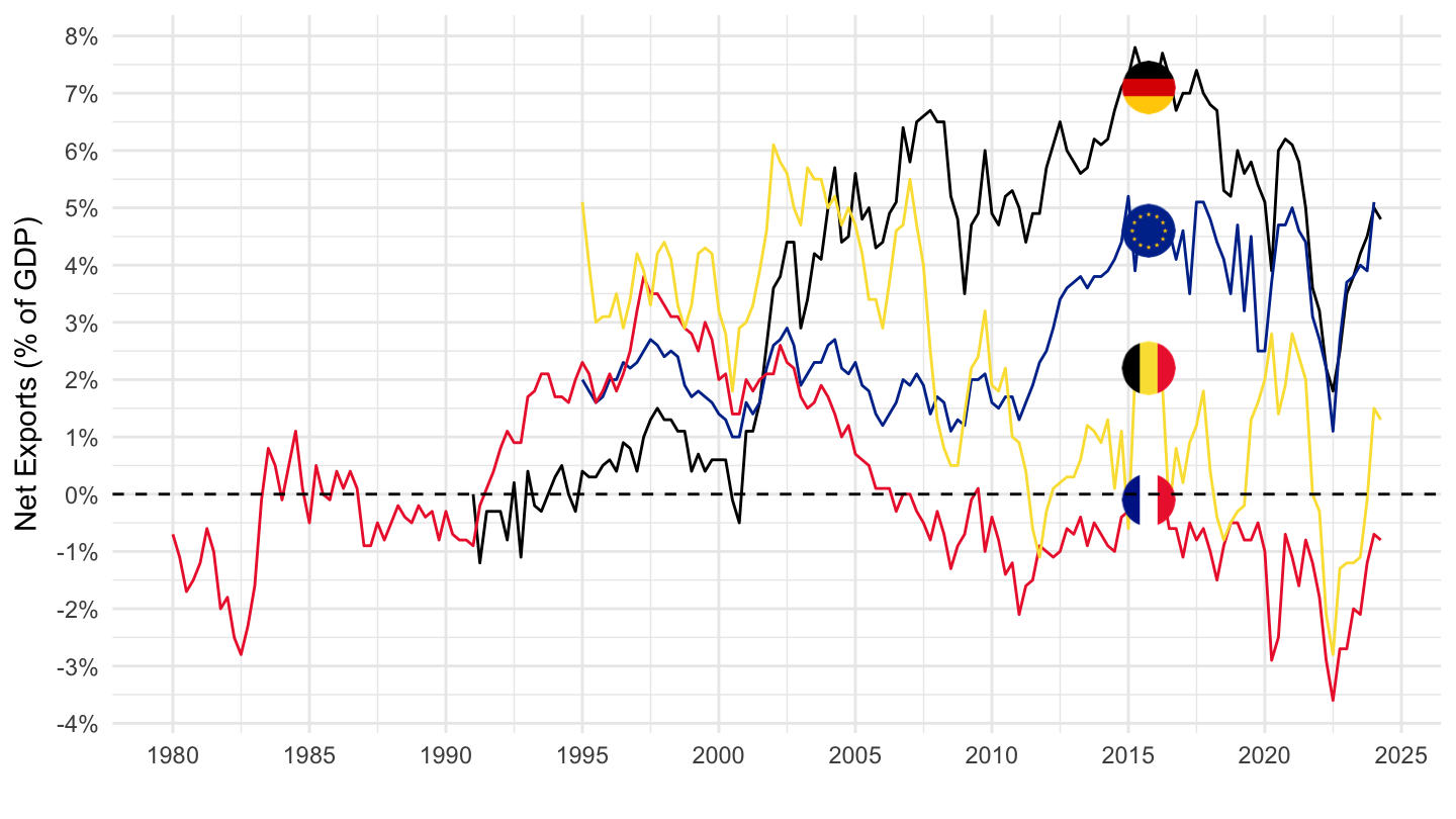
Germany, France, Eurozone
All
NSA - Unadjusted data (i.e. neither seasonally adjusted nor calendar adjusted data)
Code
namq_10_gdp %>%
  filter(na_item %in% c("P6", "P7"),
         s_adj == "NSA",
         unit == "PC_GDP",
         geo %in% c("FR", "DE", "EA")) %>%
  select(time, na_item, geo, Geo, values) %>%
  quarter_to_date %>%

  mutate(Geo= ifelse(geo == "EA", "Europe", Geo)) %>%
  spread(na_item, values) %>%
  mutate(values = (P6 - P7)/100) %>%
  left_join(colors, by = c("Geo" = "country")) %>%
  mutate(values = values) %>%
  ggplot + geom_line(aes(x = date, y = values, color = color)) +
  scale_color_identity() + theme_minimal()  +
  scale_x_date(breaks = as.Date(paste0(seq(1960, 2100, 5), "-01-01")),
               labels = date_format("%Y")) +
  add_3flags +
  theme(legend.position = "none",
        legend.title = element_blank()) +
  xlab("") + ylab("Net Exports (% of GDP)") +
  scale_y_continuous(breaks = 0.01*seq(-30, 30, 1),
                labels = percent_format(a = 1)) +
  geom_hline(yintercept = 0, linetype = "dashed",  color = "black")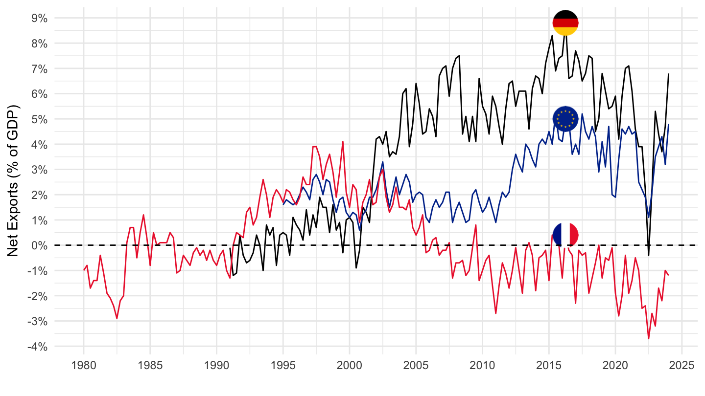
SCA
Code
namq_10_gdp %>%
  filter(na_item %in% c("P6", "P7"),
         s_adj == "SCA",
         unit == "PC_GDP",
         geo %in% c("FR", "DE", "EA")) %>%
  select(time, na_item, geo, Geo, values) %>%
  quarter_to_date %>%

  mutate(Geo= ifelse(geo == "EA", "Europe", Geo)) %>%
  spread(na_item, values) %>%
  mutate(values = (P6 - P7)/100) %>%
  left_join(colors, by = c("Geo" = "country")) %>%
  mutate(values = values) %>%
  ggplot + geom_line(aes(x = date, y = values, color = color)) +
  scale_color_identity() + theme_minimal()  +
  scale_x_date(breaks = as.Date(paste0(seq(1960, 2100, 5), "-01-01")),
               labels = date_format("%Y")) +
  add_3flags +
  theme(legend.position = "none",
        legend.title = element_blank()) +
  xlab("") + ylab("Net Exports (% of GDP)") +
  scale_y_continuous(breaks = 0.01*seq(-30, 30, 1),
                labels = percent_format(a = 1)) +
  geom_hline(yintercept = 0, linetype = "dashed",  color = "black")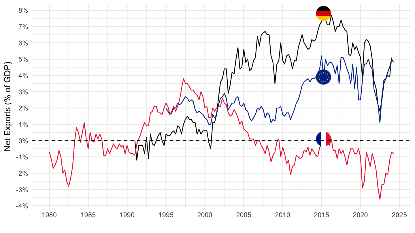
1995-
Code
namq_10_gdp %>%
  filter(na_item %in% c("P6", "P7"),
         s_adj == "SCA",
         unit == "PC_GDP",
         geo %in% c("FR", "DE", "EA")) %>%
  select(time, na_item, geo, Geo, values) %>%
  quarter_to_date %>%
  filter(date >= as.Date("1995-01-01")) %>%

  mutate(Geo= ifelse(geo == "EA", "Europe", Geo)) %>%
  spread(na_item, values) %>%
  mutate(values = (P6 - P7)/100) %>%
  left_join(colors, by = c("Geo" = "country")) %>%
  mutate(color = ifelse(geo == "EA", color2, color)) %>%
  ggplot + geom_line(aes(x = date, y = values, color = color)) +
  scale_color_identity() + theme_minimal()  + add_3flags +
  scale_x_date(breaks = as.Date(paste0(seq(1960, 2100, 5), "-01-01")),
               labels = date_format("%Y")) +
  theme(legend.position = "none",
        legend.title = element_blank()) +
  xlab("") + ylab("Exportations Nettes (% du PIB)") +
  scale_y_continuous(breaks = 0.01*seq(-30, 30, 1),
                labels = percent_format(a = 1)) +
  geom_hline(yintercept = 0, linetype = "dashed",  color = "black")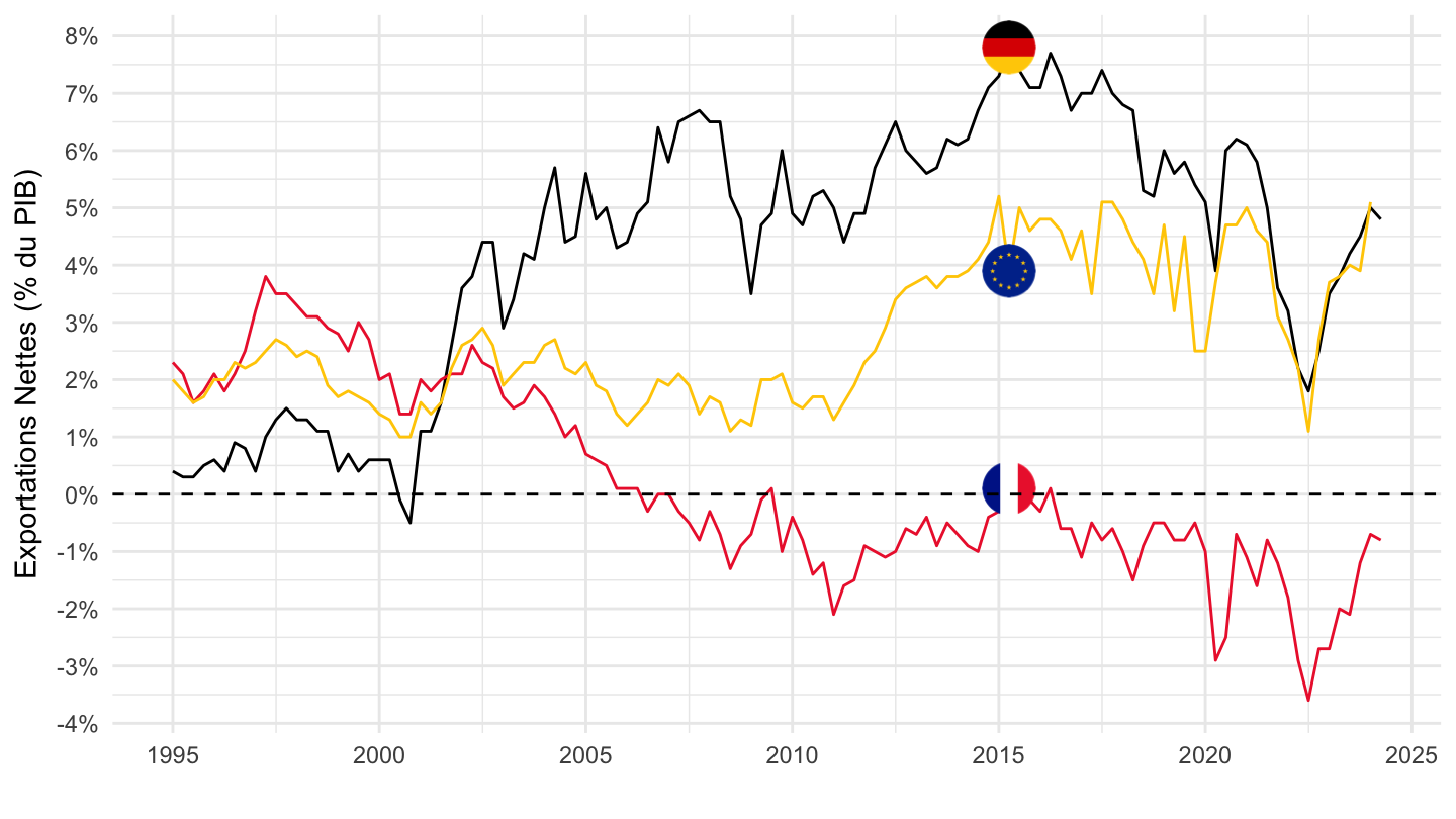
1996-
Code
namq_10_gdp %>%
  filter(na_item %in% c("P6", "P7"),
         s_adj == "NSA",
         unit == "PC_GDP",
         geo %in% c("FR", "DE", "EA")) %>%
  select(time, na_item, geo, Geo, values) %>%
  quarter_to_date %>%
  filter(date >= as.Date("1996-01-01")) %>%

  mutate(Geo= ifelse(geo == "EA", "Europe", Geo)) %>%
  spread(na_item, values) %>%
  mutate(values = (P6 - P7)/100) %>%
  left_join(colors, by = c("Geo" = "country")) %>%
  mutate(color = ifelse(geo == "EA", color2, color)) %>%
  ggplot + geom_line(aes(x = date, y = values, color = color)) +
  scale_color_identity() + theme_minimal()  + add_3flags +
  scale_x_date(breaks = as.Date(paste0(seq(1960, 2100, 2), "-01-01")),
               labels = date_format("%Y")) +
  theme(legend.position = "none",
        legend.title = element_blank()) +
  xlab("") + ylab("Net Exports (% of GDP)") +
  scale_y_continuous(breaks = 0.01*seq(-30, 30, 1),
                labels = percent_format(a = 1)) +
  geom_hline(yintercept = 0, linetype = "dashed",  color = "black")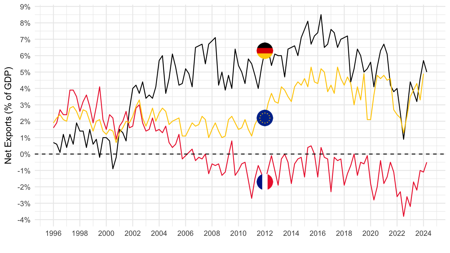
2000-
Code
namq_10_gdp %>%
  filter(na_item %in% c("P6", "P7"),
         s_adj == "NSA",
         unit == "PC_GDP",
         geo %in% c("FR", "DE", "EA")) %>%
  select(time, na_item, geo, Geo, values) %>%
  quarter_to_date %>%
  filter(date >= as.Date("2000-01-01")) %>%

  mutate(Geo= ifelse(geo == "EA", "Europe", Geo)) %>%
  spread(na_item, values) %>%
  mutate(values = (P6 - P7)/100) %>%
  left_join(colors, by = c("Geo" = "country")) %>%
  ggplot + geom_line(aes(x = date, y = values, color = color)) +
  scale_color_identity() + theme_minimal()  + add_3flags +
  scale_x_date(breaks = as.Date(paste0(seq(1960, 2100, 2), "-01-01")),
               labels = date_format("%Y")) +
  theme(legend.position = "none",
        legend.title = element_blank()) +
  xlab("") + ylab("Net Exports (% of GDP)") +
  scale_y_continuous(breaks = 0.01*seq(-30, 30, 1),
                labels = percent_format(a = 1)) +
  geom_hline(yintercept = 0, linetype = "dashed",  color = "black")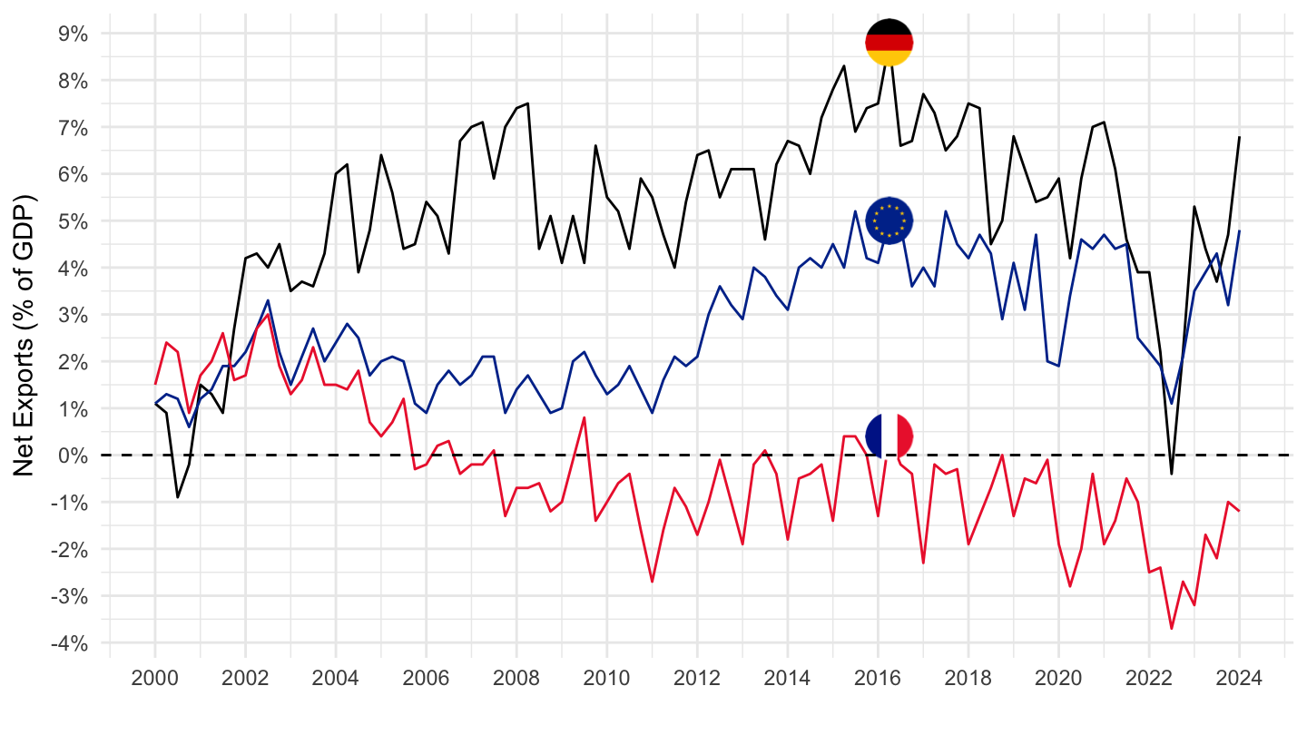
2010-
Code
namq_10_gdp %>%
  filter(na_item %in% c("P6", "P7"),
         s_adj == "NSA",
         unit == "PC_GDP",
         geo %in% c("FR", "DE", "EA")) %>%
  select(time, na_item, geo, Geo, values) %>%
  quarter_to_date %>%
  filter(date >= as.Date("2010-01-01")) %>%

  mutate(Geo= ifelse(geo == "EA", "Europe", Geo)) %>%
  spread(na_item, values) %>%
  mutate(values = (P6 - P7)/100) %>%
  left_join(colors, by = c("Geo" = "country")) %>%
  ggplot + geom_line(aes(x = date, y = values, color = color)) +
  scale_color_identity() + theme_minimal()  + add_3flags +
  scale_x_date(breaks = as.Date(paste0(seq(1960, 2100, 1), "-01-01")),
               labels = date_format("%Y")) +
  theme(legend.position = "none",
        legend.title = element_blank()) +
  xlab("") + ylab("Net Exports (% of GDP)") +
  scale_y_continuous(breaks = 0.01*seq(-30, 30, 1),
                labels = percent_format(a = 1)) +
  geom_hline(yintercept = 0, linetype = "dashed",  color = "black")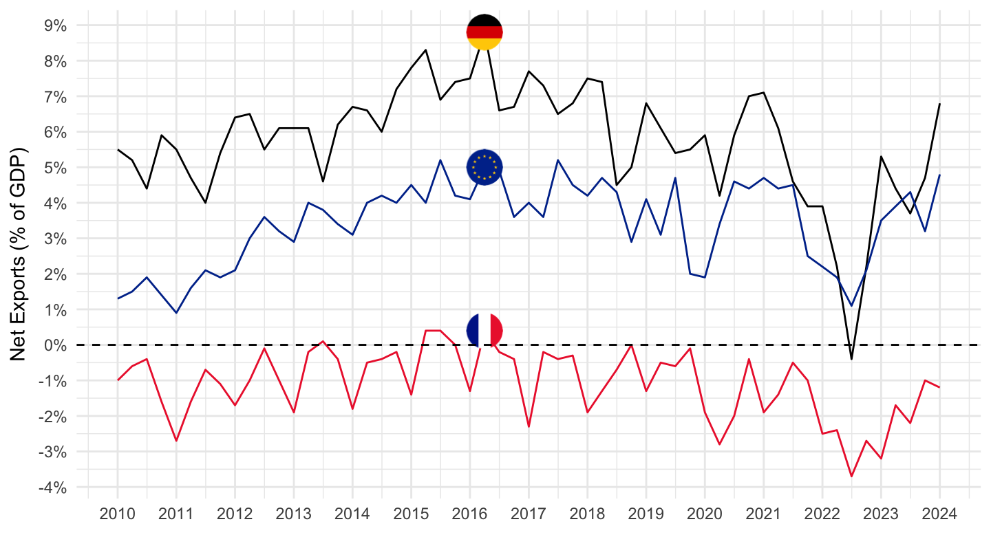
Albania, Austria, Bosnia
Code
load_data("eurostat/geo.RData")
namq_10_gdp %>%
  filter(na_item %in% c("P6", "P7"),
         s_adj == "NSA",
         unit == "PC_GDP",
         geo %in% c("AL", "AT", "BA")) %>%
  select(time, na_item, geo, Geo, values) %>%
  quarter_to_date %>%

  spread(na_item, values) %>%
  mutate(values = (P6 - P7)/100) %>%
  left_join(colors, by = c("Geo" = "country")) %>%
  ggplot + geom_line(aes(x = date, y = values, color = color)) +
  scale_color_identity() + theme_minimal()  +
  scale_x_date(breaks = as.Date(paste0(seq(1960, 2100, 5), "-01-01")),
               labels = date_format("%Y")) +
  theme(legend.position = c(0.25, 0.25),
        legend.title = element_blank()) +
  xlab("") + ylab("") +
  scale_y_continuous(breaks = 0.01*seq(-30, 30, 5),
                labels = percent_format(a = 1)) +
  geom_hline(yintercept = 0, linetype = "dashed",  color = "black")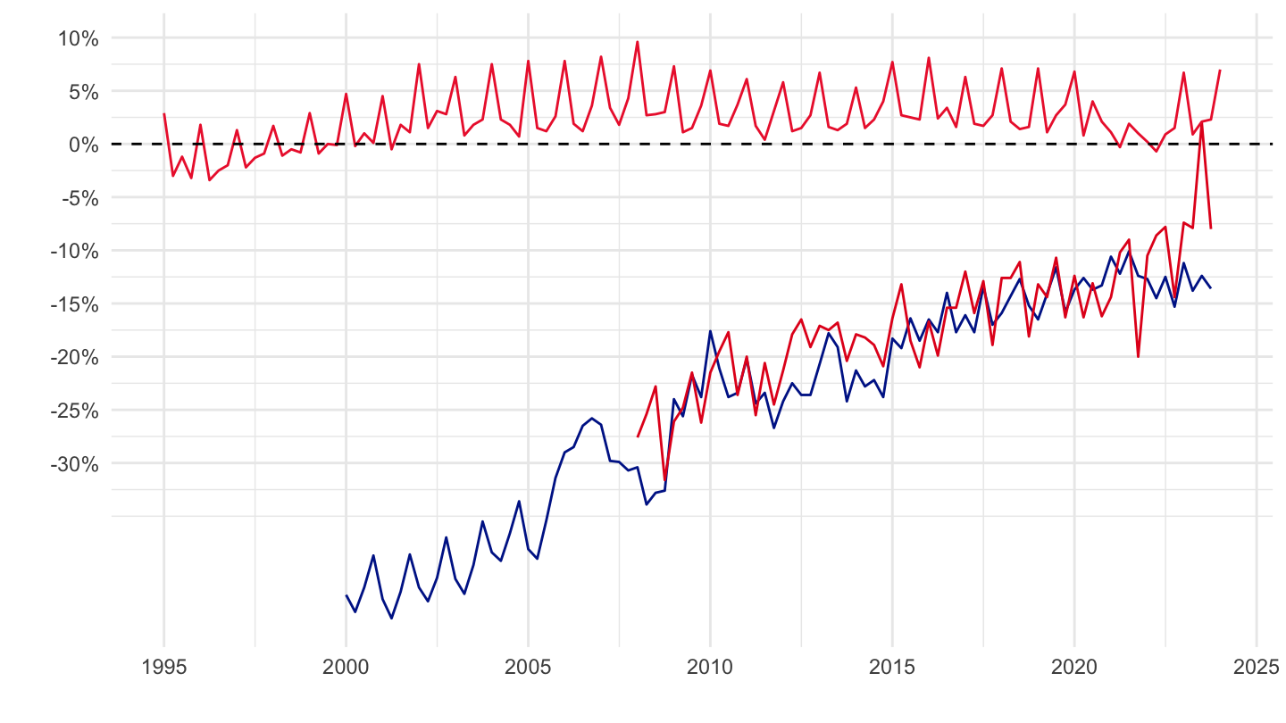
Belgium, Bulgaria, Switzerland
Code
namq_10_gdp %>%
  filter(na_item %in% c("P6", "P7"),
         s_adj == "NSA",
         unit == "PC_GDP",
         geo %in% c("BE", "BG", "CH")) %>%
  select(time, na_item, geo, Geo, values) %>%
  quarter_to_date %>%

  spread(na_item, values) %>%
  mutate(values = (P6 - P7)/100) %>%
  left_join(colors, by = c("Geo" = "country")) %>%
  ggplot + geom_line(aes(x = date, y = values, color = color)) +
  scale_color_identity() + theme_minimal()  + add_3flags +
  scale_x_date(breaks = as.Date(paste0(seq(1960, 2100, 5), "-01-01")),
               labels = date_format("%Y")) +
  theme(legend.position = c(0.25, 0.25),
        legend.title = element_blank()) +
  xlab("") + ylab("") +
  scale_y_continuous(breaks = 0.01*seq(-30, 30, 5),
                labels = percent_format(a = 1)) +
  geom_hline(yintercept = 0, linetype = "dashed",  color = "black")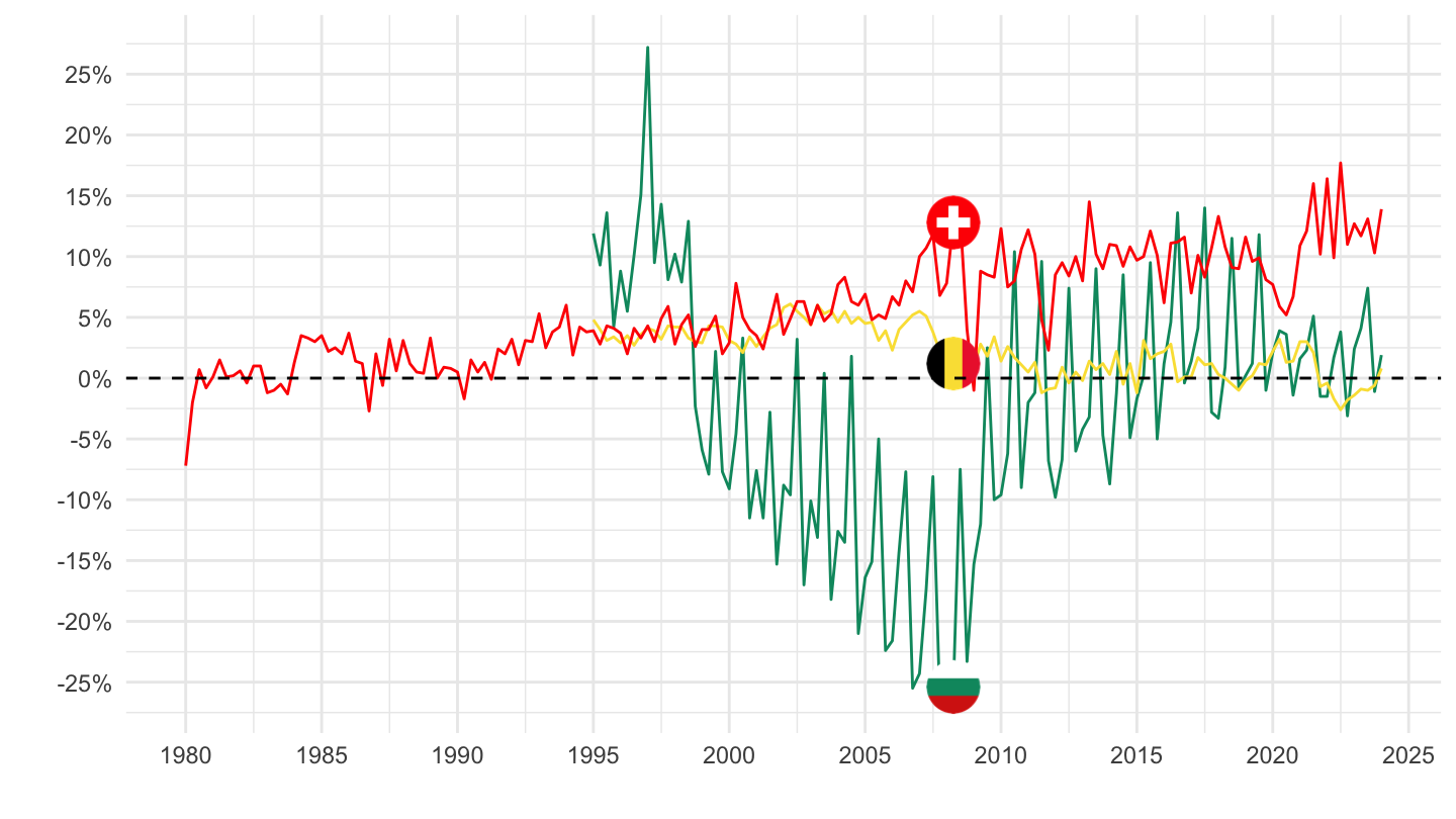
Cyprus, Czechia, Germany
Code
namq_10_gdp %>%
  filter(na_item %in% c("P6", "P7"),
         s_adj == "NSA",
         unit == "PC_GDP",
         geo %in% c("CY", "CZ", "DE")) %>%
  select(time, na_item, geo, Geo, values) %>%
  quarter_to_date %>%

  spread(na_item, values) %>%
  mutate(values = (P6 - P7)/100) %>%
  left_join(colors, by = c("Geo" = "country")) %>%
  ggplot + geom_line(aes(x = date, y = values, color = color)) +
  scale_color_identity() + theme_minimal()  + add_3flags +
  scale_x_date(breaks = as.Date(paste0(seq(1960, 2100, 5), "-01-01")),
               labels = date_format("%Y")) +
  theme(legend.position = c(0.25, 0.25),
        legend.title = element_blank()) +
  xlab("") + ylab("") +
  scale_y_continuous(breaks = 0.01*seq(-30, 30, 5),
                labels = percent_format(a = 1)) +
  geom_hline(yintercept = 0, linetype = "dashed",  color = "black")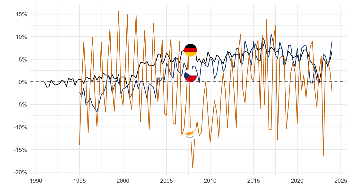
Denmark, Greece, Spain
Code
namq_10_gdp %>%
  filter(na_item %in% c("P6", "P7"),
         s_adj == "NSA",
         unit == "PC_GDP",
         geo %in% c("DK", "EL", "ES")) %>%
  select(time, na_item, geo, Geo, values) %>%
  quarter_to_date %>%

  spread(na_item, values) %>%
  mutate(values = (P6 - P7)/100) %>%
  left_join(colors, by = c("Geo" = "country")) %>%
  ggplot + geom_line(aes(x = date, y = values, color = color)) +
  scale_color_identity() + theme_minimal()  + add_3flags +
  scale_x_date(breaks = as.Date(paste0(seq(1960, 2100, 5), "-01-01")),
               labels = date_format("%Y")) +
  theme(legend.position = c(0.25, 0.95),
        legend.title = element_blank(),
        legend.direction = "horizontal") +
  xlab("") + ylab("") +
  scale_y_continuous(breaks = 0.01*seq(-30, 30, 5),
                labels = percent_format(a = 1)) +
  geom_hline(yintercept = 0, linetype = "dashed",  color = "black")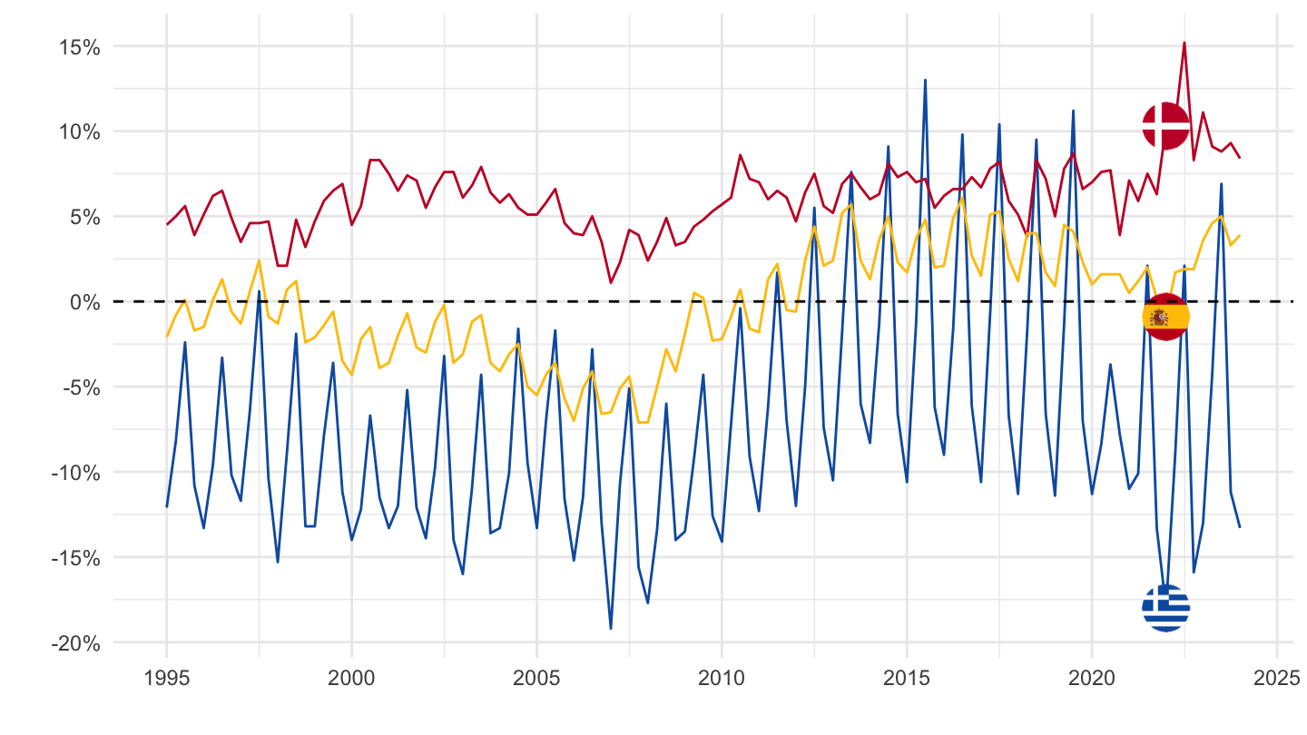
Finland, France, Croatia
Code
namq_10_gdp %>%
  filter(na_item %in% c("P6", "P7"),
         s_adj == "NSA",
         unit == "PC_GDP",
         geo %in% c("FI", "FR", "HR")) %>%
  select(time, na_item, geo, Geo, values) %>%
  quarter_to_date %>%

  spread(na_item, values) %>%
  mutate(values = (P6 - P7)/100) %>%
  left_join(colors, by = c("Geo" = "country")) %>%
  ggplot + geom_line(aes(x = date, y = values, color = color)) +
  scale_color_identity() + theme_minimal()  + add_3flags +
  scale_x_date(breaks = as.Date(paste0(seq(1960, 2100, 5), "-01-01")),
               labels = date_format("%Y")) +
  theme(legend.position = c(0.25, 0.95),
        legend.title = element_blank(),
        legend.direction = "horizontal") +
  xlab("") + ylab("") +
  scale_y_continuous(breaks = 0.01*seq(-30, 30, 5),
                labels = percent_format(a = 1)) +
  geom_hline(yintercept = 0, linetype = "dashed",  color = "black")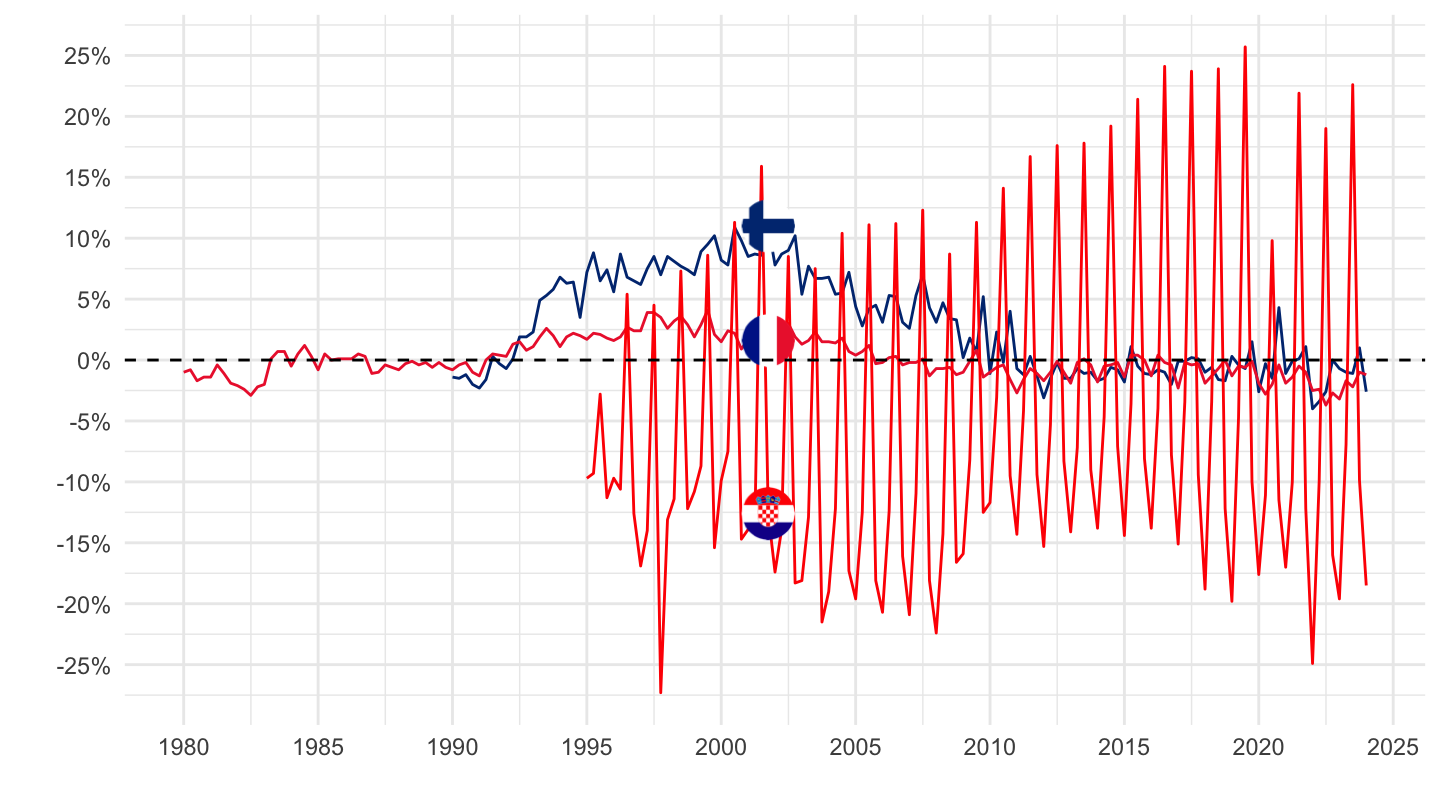
Hungary, Ireland, Iceland
Code
namq_10_gdp %>%
  filter(na_item %in% c("P6", "P7"),
         s_adj == "NSA",
         unit == "PC_GDP",
         geo %in% c("HU", "IE", "IS")) %>%
  select(time, na_item, geo, Geo, values) %>%
  quarter_to_date %>%

  spread(na_item, values) %>%
  mutate(values = (P6 - P7)/100) %>%
  left_join(colors, by = c("Geo" = "country")) %>%
  ggplot + geom_line(aes(x = date, y = values, color = color)) +
  scale_color_identity() + theme_minimal()  + add_3flags +
  scale_x_date(breaks = as.Date(paste0(seq(1960, 2100, 5), "-01-01")),
               labels = date_format("%Y")) +
  theme(legend.position = c(0.25, 0.95),
        legend.title = element_blank(),
        legend.direction = "horizontal") +
  xlab("") + ylab("") +
  scale_y_continuous(breaks = 0.01*seq(-30, 100, 5),
                labels = percent_format(a = 1)) +
  geom_hline(yintercept = 0, linetype = "dashed",  color = "black")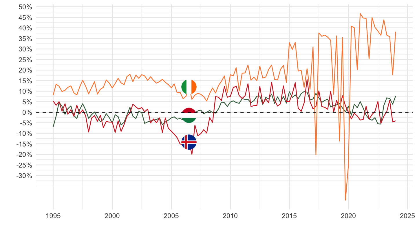
Italy, Lithuania, Luxembourg
Code
namq_10_gdp %>%
  filter(na_item %in% c("P6", "P7"),
         s_adj == "SCA",
         unit == "PC_GDP",
         geo %in% c("IT", "LT", "LU")) %>%
  select(time, na_item, geo, Geo, values) %>%
  quarter_to_date %>%

  spread(na_item, values) %>%
  mutate(values = (P6 - P7)/100) %>%
  left_join(colors, by = c("Geo" = "country")) %>%
  ggplot + geom_line(aes(x = date, y = values, color = color)) +
  scale_color_identity() + theme_minimal()  + add_3flags +
  scale_x_date(breaks = as.Date(paste0(seq(1960, 2100, 5), "-01-01")),
               labels = date_format("%Y")) +
  theme(legend.position = c(0.25, 0.95),
        legend.title = element_blank(),
        legend.direction = "horizontal") +
  xlab("") + ylab("") +
  scale_y_continuous(breaks = 0.01*seq(-30, 100, 5),
                labels = percent_format(a = 1)) +
  geom_hline(yintercept = 0, linetype = "dashed",  color = "black")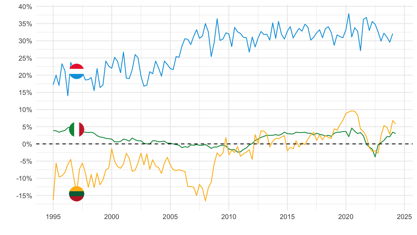
Germany, France, Italy
NSA
Code
namq_10_gdp %>%
  filter(na_item %in% c("P6", "P7"),
         s_adj == "NSA",
         unit == "PC_GDP",
         geo %in% c("FR", "DE", "IT")) %>%
  select(time, na_item, geo, Geo, values) %>%
  quarter_to_date %>%

  spread(na_item, values) %>%
  mutate(values = (P6 - P7)/100) %>%
  left_join(colors, by = c("Geo" = "country")) %>%
  ggplot + geom_line(aes(x = date, y = values, color = color)) +
  scale_color_identity() + theme_minimal()  + add_3flags +
  scale_x_date(breaks = as.Date(paste0(seq(1960, 2100, 5), "-01-01")),
               labels = date_format("%Y")) +
  theme(legend.position = c(0.35, 0.85),
        legend.title = element_blank()) +
  xlab("") + ylab("") +
  scale_y_continuous(breaks = 0.01*seq(-30, 30, 1),
                labels = percent_format(a = 1)) +
  geom_hline(yintercept = 0, linetype = "dashed",  color = "black")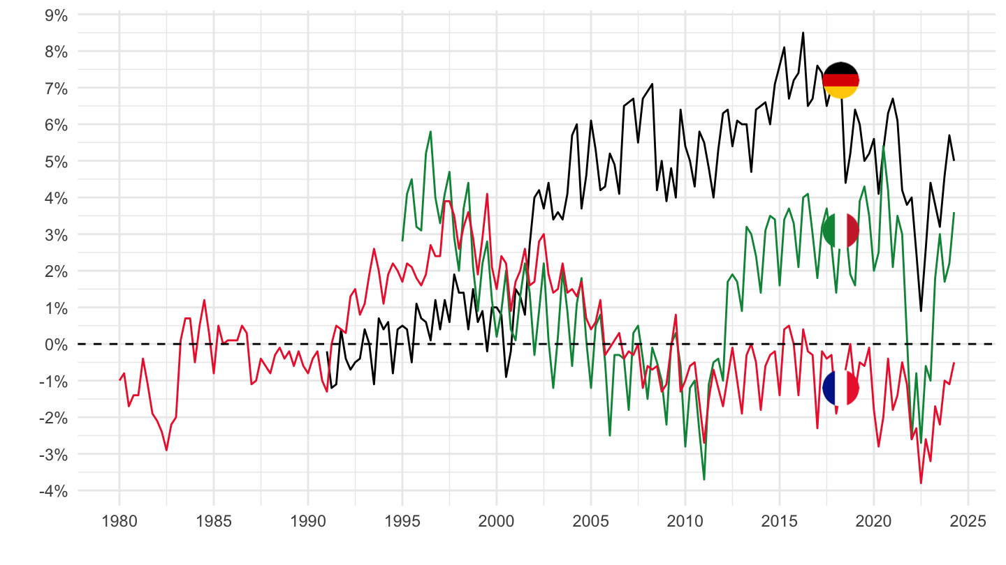
SCA
Code
namq_10_gdp %>%
  filter(na_item %in% c("P6", "P7"),
         s_adj == "SCA",
         unit == "PC_GDP",
         geo %in% c("FR", "DE", "IT")) %>%
  select(time, na_item, geo, Geo, values) %>%
  quarter_to_date %>%

  spread(na_item, values) %>%
  mutate(values = (P6 - P7)/100) %>%
  left_join(colors, by = c("Geo" = "country")) %>%

  ggplot + geom_line(aes(x = date, y = values, color = color)) +
  scale_color_identity() + theme_minimal()  +
  scale_x_date(breaks = as.Date(paste0(seq(1960, 2100, 5), "-01-01")),
               labels = date_format("%Y")) + add_3flags +
  theme(legend.position = c(0.35, 0.85),
        legend.title = element_blank()) +
  xlab("") + ylab("") +
  scale_y_continuous(breaks = 0.01*seq(-30, 30, 1),
                labels = percent_format(a = 1)) +
  geom_hline(yintercept = 0, linetype = "dashed",  color = "black")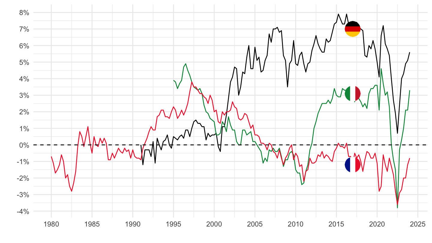
Germany, France, Italy, Spain, Eurozone
SCA
Code
namq_10_gdp %>%
  filter(na_item %in% c("P6", "P7"),
         s_adj == "SCA",
         unit == "PC_GDP",
         geo %in% c("FR", "DE", "IT", "EA", "ES")) %>%
  select(time, na_item, geo, Geo, values) %>%
  quarter_to_date %>%

  spread(na_item, values) %>%
  mutate(values = (P6 - P7)/100) %>%
  filter(date >= as.Date("1998-01-01")) %>%
  mutate(Geo= ifelse(geo == "EA", "Europe", Geo)) %>%
  left_join(colors, by = c("Geo" = "country")) %>%

  ggplot + geom_line(aes(x = date, y = values, color = color)) +
  scale_color_identity() + theme_minimal()  +
  scale_x_date(breaks = as.Date(paste0(seq(1960, 2100, 2), "-01-01")),
               labels = date_format("%Y")) + add_5flags +
  theme(legend.position = c(0.35, 0.85),
        legend.title = element_blank()) +
  xlab("") + ylab("") +
  scale_y_continuous(breaks = 0.01*seq(-30, 30, 1),
                labels = percent_format(a = 1)) +
  geom_hline(yintercept = 0, linetype = "dashed",  color = "black")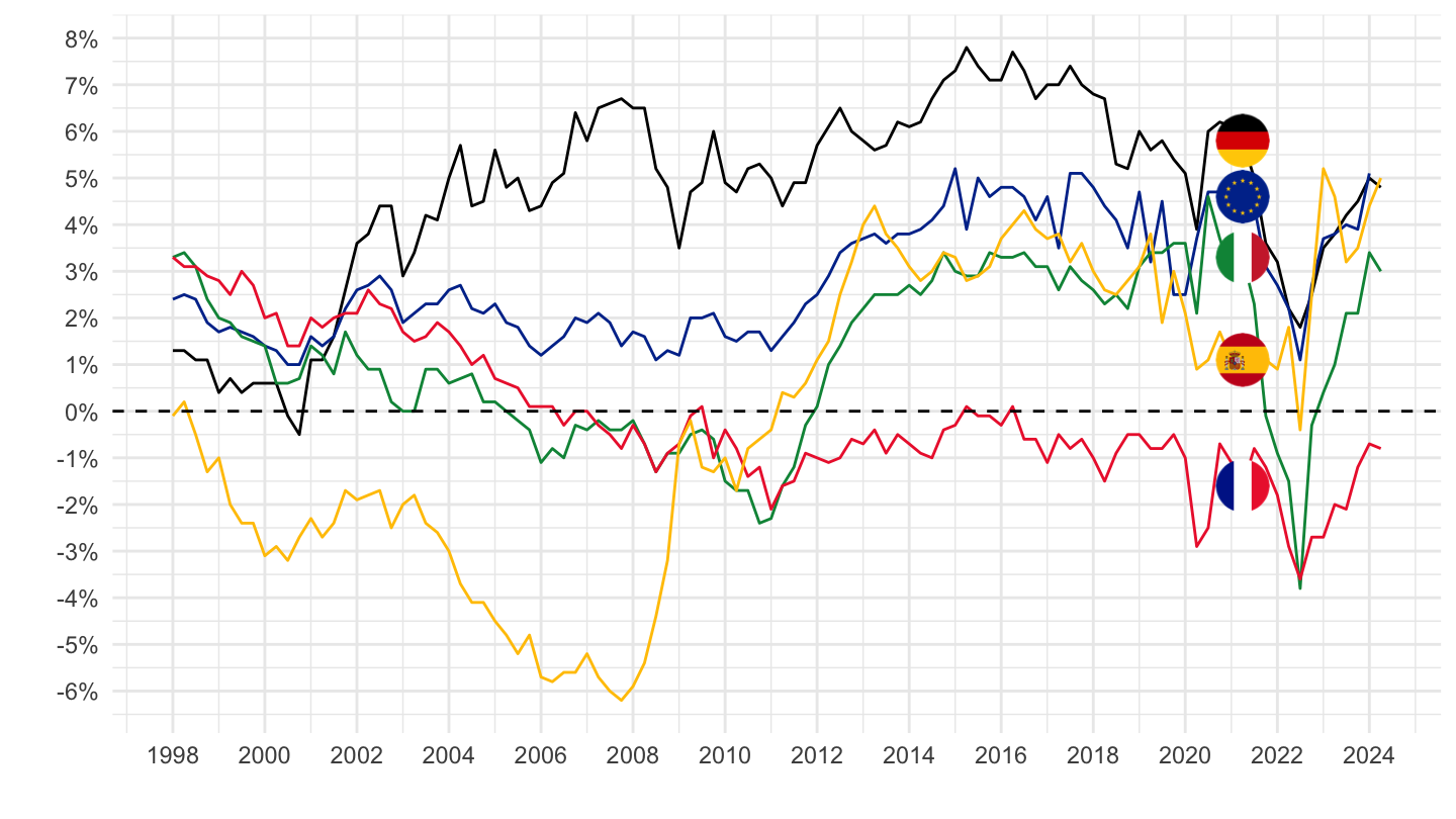
Poland, France, Italy
Code
namq_10_gdp %>%
  filter(na_item %in% c("P6", "P7"),
         s_adj == "NSA",
         unit == "PC_GDP",
         geo %in% c("PL", "DE", "IT")) %>%
  select(time, na_item, geo, Geo, values) %>%
  quarter_to_date %>%

  spread(na_item, values) %>%
  mutate(values = (P6 - P7)/100) %>%
  left_join(colors, by = c("Geo" = "country")) %>%

  ggplot + geom_line(aes(x = date, y = values, color = color)) +
  scale_color_identity() + theme_minimal()  +
  scale_x_date(breaks = as.Date(paste0(seq(1960, 2100, 5), "-01-01")),
               labels = date_format("%Y")) + add_3flags +
  theme(legend.position = c(0.35, 0.85),
        legend.title = element_blank()) +
  xlab("") + ylab("") +
  scale_y_continuous(breaks = 0.01*seq(-30, 30, 1),
                labels = percent_format(a = 1)) +
  geom_hline(yintercept = 0, linetype = "dashed",  color = "black")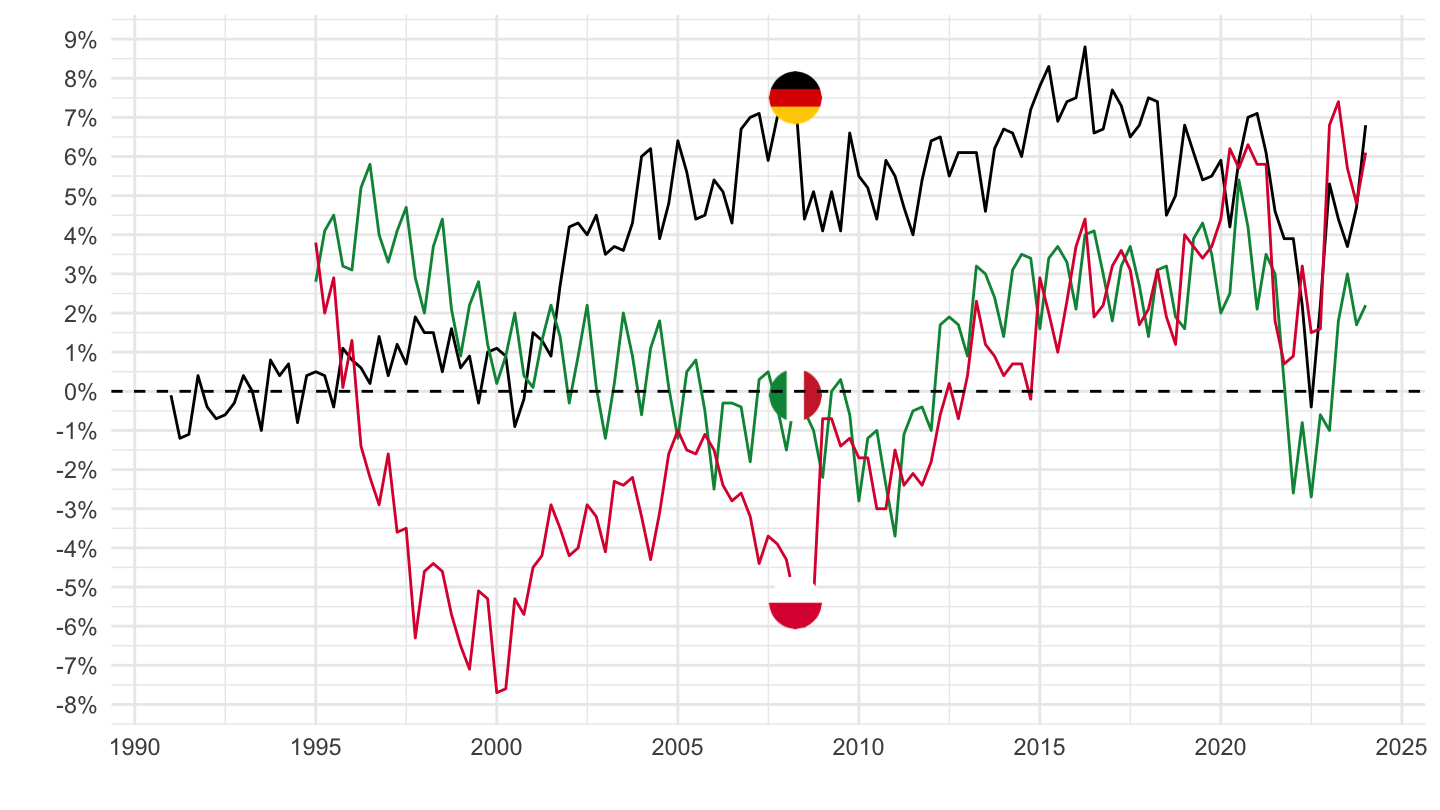
Poland, Austria, Germany, Tchequia, Hungary, Slovakia
Code
namq_10_gdp %>%
  filter(na_item %in% c("P6", "P7"),
         s_adj == "NSA",
         unit == "PC_GDP",
         geo %in% c("PL", "DE", "SK", "CZ", "HU", "AT")) %>%
  select(time, na_item, geo, Geo, values) %>%
  quarter_to_date %>%

  spread(na_item, values) %>%
  mutate(values = (P6 - P7)/100) %>%
  left_join(colors, by = c("Geo" = "country")) %>%

  ggplot + geom_line(aes(x = date, y = values, color = color)) +
  scale_color_identity() + theme_minimal()  +
  scale_x_date(breaks = as.Date(paste0(seq(1960, 2100, 5), "-01-01")),
               labels = date_format("%Y")) + add_6flags +
  theme(legend.position = c(0.85, 0.25),
        legend.title = element_blank()) +
  xlab("") + ylab("") +
  scale_y_continuous(breaks = 0.01*seq(-30, 30, 5),
                labels = percent_format(a = 1)) +
  geom_hline(yintercept = 0, linetype = "dashed",  color = "black")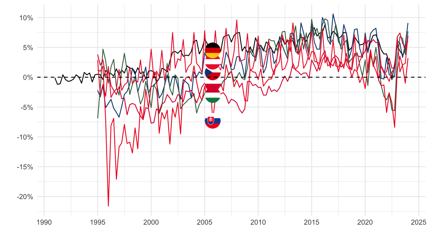
Decompose GDP
Bn - 2019Q1 - France, Italy, Germany, Spain
Code
namq_10_gdp %>%
  filter(s_adj == "SCA",
         # CLV10_MEUR: Chain linked volumes (2010), million euro
         unit == "CLV10_MEUR",
         time %in% c("2019Q1"),
         geo %in% c("FR", "IT", "DE", "ES")) %>%

  select(na_item, Na_item, geo, values) %>%
  spread(geo, values) %>%
  {if (is_html_output()) datatable(., filter = 'top', rownames = F) else .}
% of GDP - 2019Q1 - France, Italy, Germany, Spain
Code
namq_10_gdp %>%
  filter(s_adj == "SCA",
         unit == "PC_GDP",
         time %in% c("2019Q1"),
         geo %in% c("FR", "IT", "DE", "ES")) %>%

  select(na_item, Na_item, geo, values) %>%
  mutate(values = values %>% paste0("%")) %>%
  spread(geo, values) %>%
  {if (is_html_output()) datatable(., filter = 'top', rownames = F) else .}
% - 2019Q1 - France, Italy, Germany, Spain
Code
namq_10_gdp %>%
  filter(s_adj == "SCA",
         # CLV10_MEUR: Chain linked volumes (2010), million euro
         unit == "CP_MEUR",
         time %in% c("2019Q1"),
         geo %in% c("FR", "IT", "DE", "ES")) %>%

  select(na_item, Na_item, geo, values) %>%
  group_by(geo) %>%
  mutate(values = round(100*values/values[na_item == "B1GQ"], 1) %>% paste0("%")) %>%
  spread(geo, values) %>%
  {if (is_html_output()) datatable(., filter = 'top', rownames = F) else .}
France - 1979, 1989, 1999, 2009, 2019
Code
namq_10_gdp %>%
  filter(s_adj == "SCA",
         # CLV10_MEUR: Chain linked volumes (2010), million euro
         unit == "CP_MEUR",
         time %in% c("2019Q1", "2009Q1", "1999Q1", "1989Q1", "1979Q1"),
         geo %in% c("FR")) %>%

  select(na_item, Na_item, time, values) %>%
  group_by(time) %>%
  mutate(values = round(100*values/values[na_item == "B1GQ"], 1) %>% paste0("%")) %>%
  spread(time, values) %>%
  {if (is_html_output()) datatable(., filter = 'top', rownames = F) else .}
REAL Gross Domestic Product
Allemagne, France, Europe, Italy
1990-
Code
namq_10_gdp %>%
  filter(geo %in% c("EA19", "DE", "IT", "FR"),
         # B1GQ: Gross domestic product at market prices
         na_item == "B1GQ",
         # SCA: Seasonally and calendar adjusted data
         s_adj == "SCA",
         # CLV10_MEUR: Chain linked volumes (2010), million euro
         unit == "CLV10_MEUR") %>%
  quarter_to_date %>%
  filter(date >= as.Date("1990-01-01")) %>%

  mutate(Geo = ifelse(geo == "EA19", "Europe", Geo)) %>%
  group_by(geo) %>%
  mutate(values = 100*values / values[1]) %>%
  left_join(colors, by = c("Geo" = "country")) %>%
  ggplot + geom_line(aes(x = date, y = values, color = color)) +
  scale_color_identity() + theme_minimal() + xlab("") + ylab("") +
  scale_x_date(breaks = as.Date(paste0(seq(1960, 2100, 5), "-01-01")),
               labels = date_format("%Y")) +
  add_4flags +
  theme(legend.position = c(0.35, 0.85),
        legend.title = element_blank()) +
  scale_y_log10(breaks = seq(80, 180, 5),
                labels = dollar_format(suffix = "", prefix = "", accuracy = 1))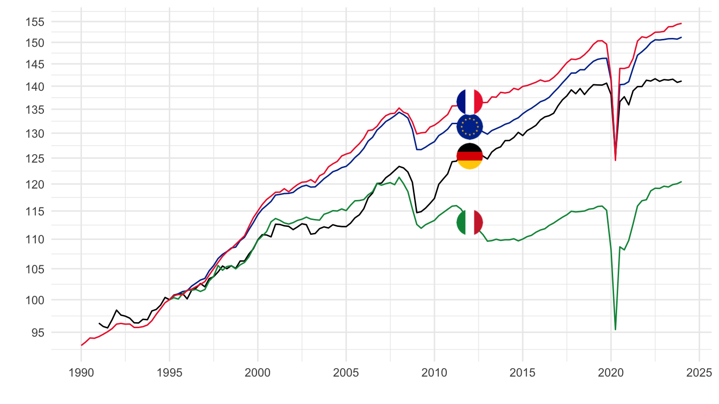
1995-
Code
namq_10_gdp %>%
  filter(geo %in% c("EA19", "DE", "IT", "FR"),
         # B1GQ: Gross domestic product at market prices
         na_item == "B1GQ",
         # SCA: Seasonally and calendar adjusted data
         s_adj == "SCA",
         # CLV10_MEUR: Chain linked volumes (2010), million euro
         unit == "CLV10_MEUR") %>%
  quarter_to_date %>%
  filter(date >= as.Date("1995-01-01")) %>%

  mutate(Geo = ifelse(geo == "EA19", "Europe", Geo)) %>%
  group_by(geo) %>%
  mutate(values = 100*values / values[1]) %>%
  left_join(colors, by = c("Geo" = "country")) %>%
  ggplot + geom_line(aes(x = date, y = values, color = color)) +
  scale_color_identity() + theme_minimal() + xlab("") + ylab("") +
  scale_x_date(breaks = as.Date(paste0(seq(1960, 2100, 5), "-01-01")),
               labels = date_format("%Y")) +
  add_4flags +
  theme(legend.position = c(0.35, 0.85),
        legend.title = element_blank()) +
  scale_y_log10(breaks = seq(80, 180, 5),
                labels = dollar_format(suffix = "", prefix = "", accuracy = 1))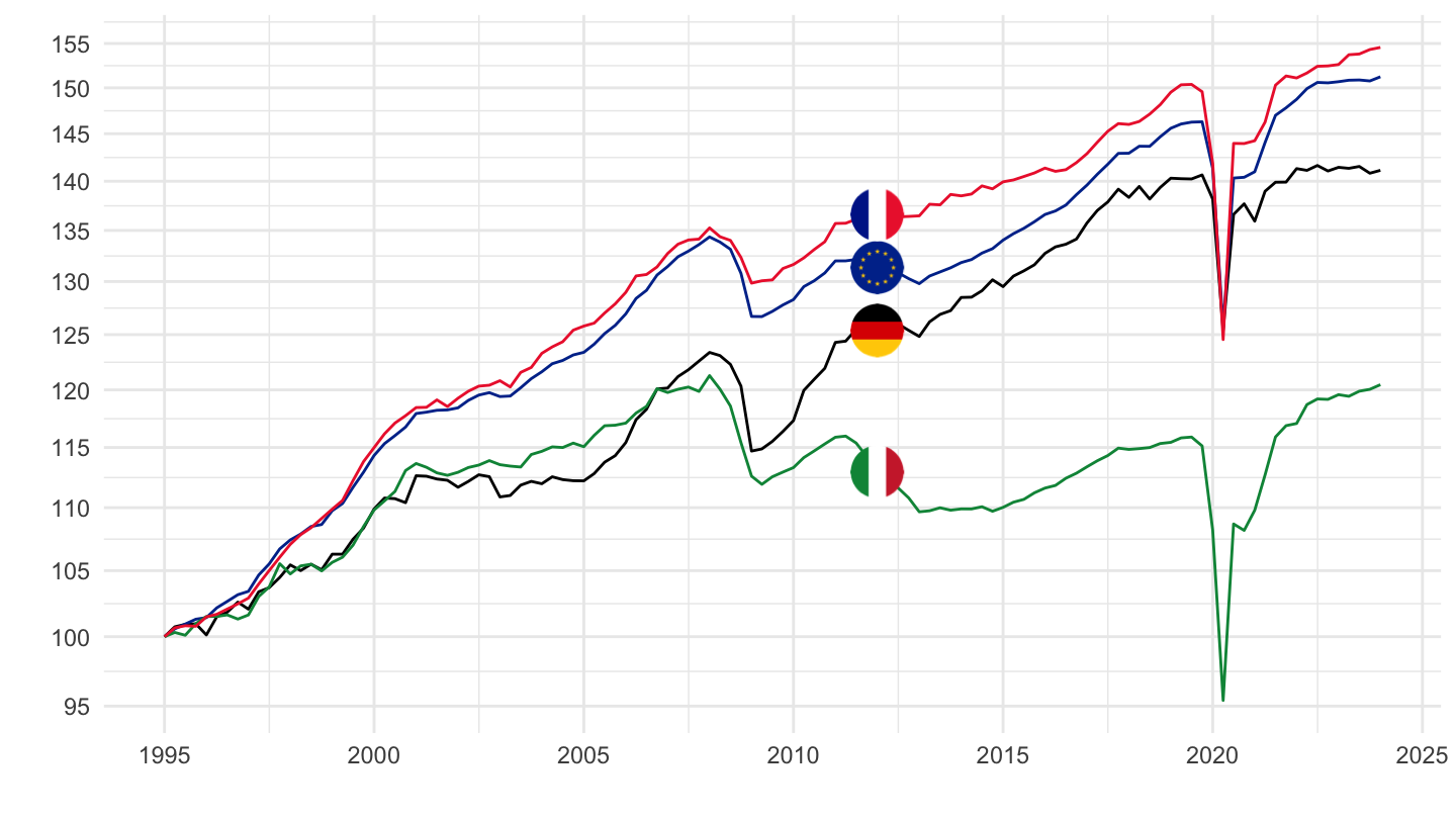
1996-
Code
namq_10_gdp %>%
  filter(geo %in% c("EA19", "DE", "IT", "FR"),
         # B1GQ: Gross domestic product at market prices
         na_item == "B1GQ",
         # SCA: Seasonally and calendar adjusted data
         s_adj == "SCA",
         # CLV10_MEUR: Chain linked volumes (2010), million euro
         unit == "CLV10_MEUR") %>%
  quarter_to_date %>%
  filter(date >= as.Date("1996-01-01")) %>%

  mutate(Geo = ifelse(geo == "EA19", "Europe", Geo)) %>%
  group_by(geo) %>%
  mutate(values = 100*values / values[1]) %>%
  left_join(colors, by = c("Geo" = "country")) %>%
  ggplot + geom_line(aes(x = date, y = values, color = color)) +
  scale_color_identity() + theme_minimal() + xlab("") + ylab("") +
  scale_x_date(breaks = as.Date(paste0(seq(1960, 2100, 2), "-01-01")),
               labels = date_format("%Y")) +
  add_4flags +
  theme(legend.position = c(0.35, 0.85),
        legend.title = element_blank()) +
  scale_y_log10(breaks = seq(80, 180, 5),
                labels = dollar_format(suffix = "", prefix = "", accuracy = 1))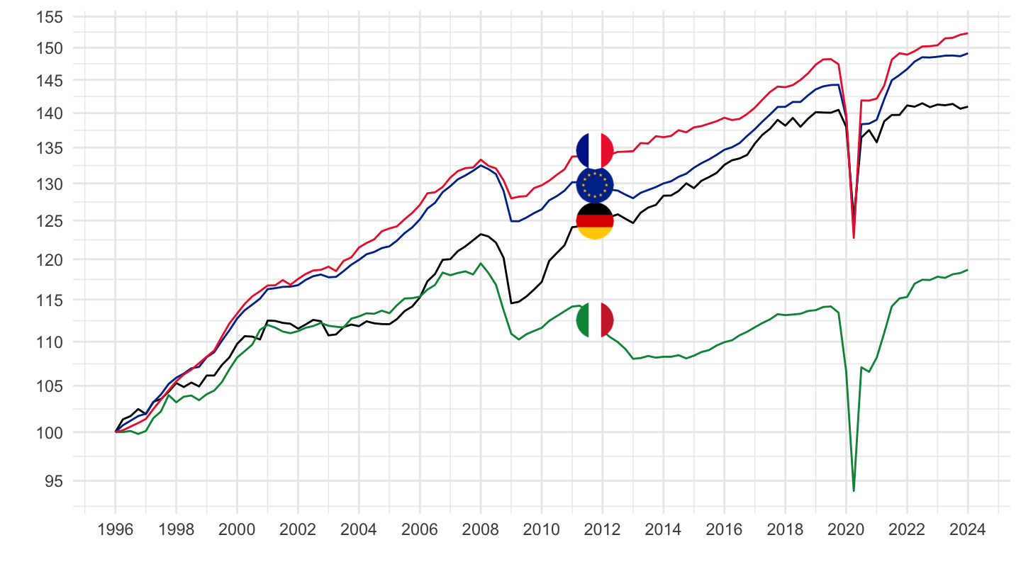
2000-
Code
namq_10_gdp %>%
  filter(geo %in% c("EA19", "DE", "IT", "FR"),
         # B1GQ: Gross domestic product at market prices
         na_item == "B1GQ",
         # SCA: Seasonally and calendar adjusted data
         s_adj == "SCA",
         # CLV10_MEUR: Chain linked volumes (2010), million euro
         unit == "CLV10_MEUR") %>%
  quarter_to_date %>%
  filter(date >= as.Date("2000-01-01")) %>%

  mutate(Geo = ifelse(geo == "EA19", "Europe", Geo)) %>%
  group_by(geo) %>%
  mutate(values = 100*values / values[date == as.Date("2000-01-01")]) %>%
  left_join(colors, by = c("Geo" = "country")) %>%
  ggplot + geom_line(aes(x = date, y = values, color = color)) +
  scale_color_identity() + theme_minimal() + xlab("") + ylab("") +
  scale_x_date(breaks = as.Date(paste0(seq(1960, 2100, 2), "-01-01")),
               labels = date_format("%Y")) +
  add_4flags +
  theme(legend.position = c(0.35, 0.85),
        legend.title = element_blank()) +
  scale_y_log10(breaks = seq(80, 130, 5),
                labels = dollar_format(suffix = "", prefix = "", accuracy = 1))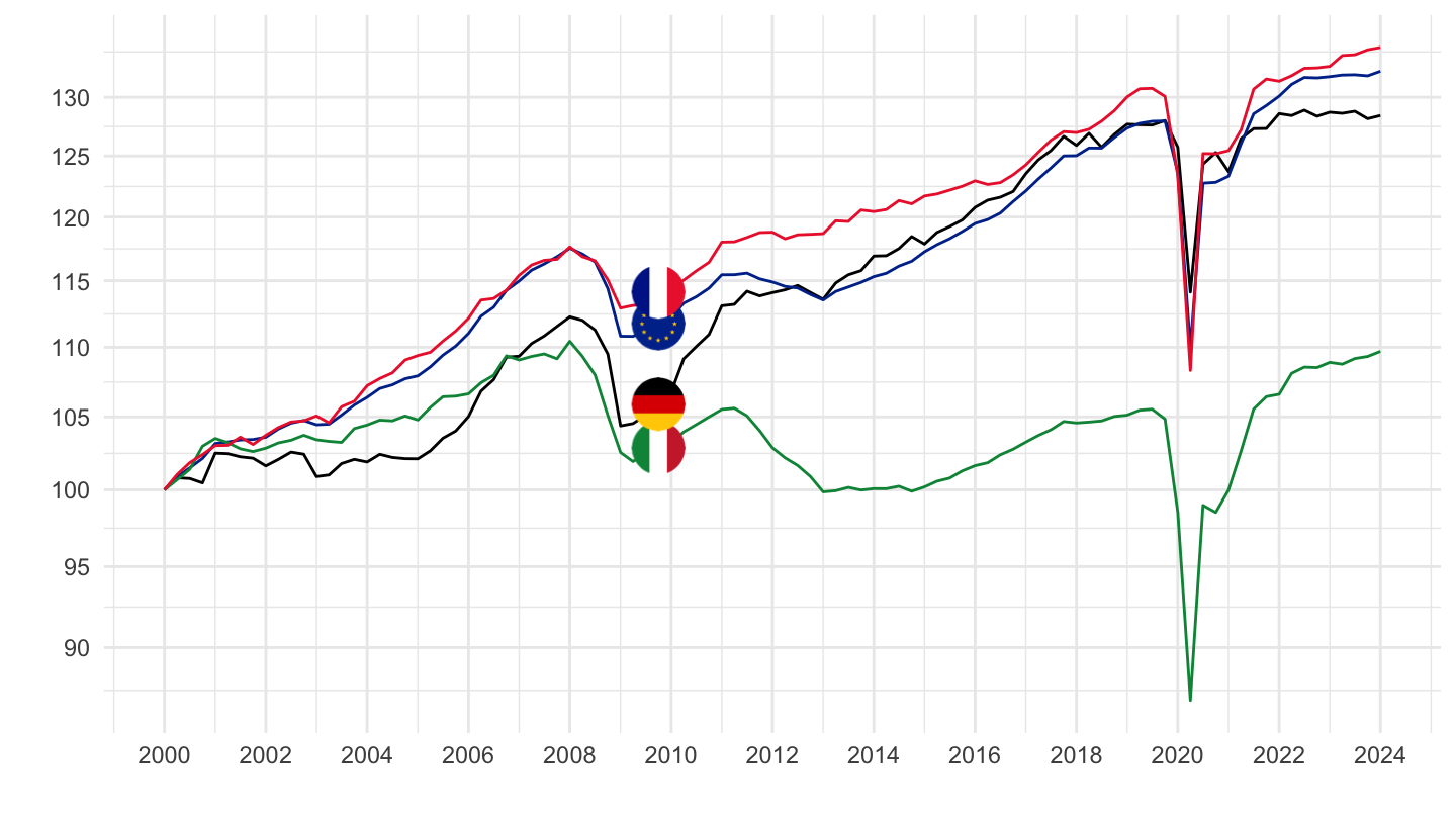
2017-
Code
namq_10_gdp %>%
  filter(geo %in% c("EA19", "DE", "IT", "FR"),
         # B1GQ: Gross domestic product at market prices
         na_item == "B1GQ",
         # SCA: Seasonally and calendar adjusted data
         s_adj == "SCA",
         # CLV10_MEUR: Chain linked volumes (2010), million euro
         unit == "CLV10_MEUR") %>%
  quarter_to_date %>%
  filter(date >= as.Date("2017-01-01")) %>%

  mutate(Geo = ifelse(geo == "EA19", "Europe", Geo)) %>%
  group_by(geo) %>%
  mutate(values = 100*values / values[date == as.Date("2017-01-01")]) %>%
  left_join(colors, by = c("Geo" = "country")) %>%
  mutate(date = zoo::as.yearqtr(paste0(year(date), " Q", quarter(date)))) %>%
  ggplot + geom_line(aes(x = date, y = values, color = color)) +
  scale_color_identity() + theme_minimal() + xlab("") + ylab("") +
  zoo::scale_x_yearqtr(labels = date_format("%Y Q%q"),
                       breaks = seq(zoo::as.yearqtr("2017 Q1"), zoo::as.yearqtr("2100 Q1"), by = 0.25)) +
  add_4flags +
  theme(legend.position = c(0.35, 0.85),
        legend.title = element_blank(),
        axis.text.x = element_text(angle = 45, vjust = 1, hjust = 1)) +
  scale_y_log10(breaks = seq(80, 130, 2),
                labels = dollar_format(suffix = "", prefix = "", accuracy = 1))
2019Q4-
Code
namq_10_gdp %>%
  filter(geo %in% c("EA20", "DE", "IT", "FR", "IE"),
         # B1GQ: Gross domestic product at market prices
         na_item == "B1GQ",
         time %in% c("2019Q4", "2023Q4"),
         # SCA: Seasonally and calendar adjusted data
         s_adj == "SCA",
         # CLV10_MEUR: Chain linked volumes (2010), million euro
         unit == "CLV15_MEUR") %>%

  select(geo, Geo, values, time) %>%
  mutate(values = values/1000) %>%
  spread(time, values) %>%
  mutate(Change = `2023Q4` - `2019Q4`) %>%
print_table_conditional| geo | Geo | 2019Q4 | 2023Q4 | Change |
|---|---|---|---|---|
| DE | Germany | 829.2284 | 830.9949 | 1.7665 |
| EA20 | Euro area – 20 countries (2023-2025) | 2885.1528 | 3004.0807 | 118.9279 |
| FR | France | 587.0422 | 612.7374 | 25.6952 |
| IE | Ireland | 87.8725 | 108.6072 | 20.7347 |
| IT | Italy | 431.6323 | 456.5300 | 24.8977 |
Allemagne, France, Italie
All
Code
namq_10_gdp %>%
  filter(geo %in% c("FR", "DE", "IT"),
         # B1GQ: Gross domestic product at market prices
         na_item == "B1GQ",
         # SCA: Seasonally and calendar adjusted data
         s_adj == "SCA",
         # CLV10_MEUR: Chain linked volumes (2010), million euro
         unit == "CLV10_MEUR") %>%
  quarter_to_date %>%

  left_join(colors, by = c("Geo" = "country")) %>%
  mutate(values = values/1000) %>%
  ggplot + geom_line(aes(x = date, y = values, color = color)) +
  scale_color_identity() + theme_minimal() + xlab("") + ylab("") + add_3flags +
  scale_x_date(breaks = as.Date(paste0(seq(1960, 2100, 5), "-01-01")),
               labels = date_format("%Y")) +
  theme(legend.position = c(0.35, 0.85),
        legend.title = element_blank()) +
  scale_y_log10(breaks = seq(0, 1000, 100),
                labels = dollar_format(suffix = " Bn€", prefix = "", accuracy = 1))
1995-
Code
namq_10_gdp %>%
  filter(geo %in% c("FR", "DE", "IT"),
         # B1GQ: Gross domestic product at market prices
         na_item == "B1GQ",
         # SCA: Seasonally and calendar adjusted data
         s_adj == "SCA",
         # CLV10_MEUR: Chain linked volumes (2010), million euro
         unit == "CLV10_MEUR") %>%
  quarter_to_date %>%
  filter(date >= as.Date("1995-01-01")) %>%

  left_join(colors, by = c("Geo" = "country")) %>%
  mutate(values = values/1000) %>%
  ggplot + geom_line(aes(x = date, y = values, color = color)) +
  scale_color_identity() + theme_minimal() + xlab("") + ylab("") + add_3flags +
  scale_x_date(breaks = as.Date(paste0(seq(1960, 2100, 5), "-01-01")),
               labels = date_format("%Y")) +
  theme(legend.position = c(0.35, 0.85),
        legend.title = element_blank()) +
  scale_y_log10(breaks = seq(0, 1000, 100),
                labels = dollar_format(suffix = " Bn€", prefix = "", accuracy = 1))
2019Q4 to 2020Q1
Code
load_data("eurostat/geo.RData")
namq_10_gdp %>%
  filter(na_item == "B1GQ",
         # SCA: Seasonally and calendar adjusted data
         s_adj == "SCA",
         # CLV10_MEUR: Chain linked volumes (2010), million euro
         unit == "CLV10_MEUR",
         time %in% c("2020Q1", "2019Q4")) %>%

  select(geo, Geo, time, values) %>%
  spread(time, values) %>%
  transmute(geo, Geo,
            `growth (%)` = round(100*(`2020Q1`/`2019Q4` - 1), 1)) %>%
  mutate(Geo = ifelse(geo == "DE", "Germany", Geo)) %>%
  mutate(Flag = gsub(" ", "-", str_to_lower(Geo)),
         Flag = paste0('<img src="../../icon/flag/vsmall/', Flag, '.png" alt="Flag">')) %>%
  select(Flag, everything()) %>%
  {if (is_html_output()) datatable(., filter = 'top', rownames = F, escape = F) else .}
2019Q4 to 2020Q1 to 2021Q4
Code
load_data("eurostat/geo.RData")
namq_10_gdp %>%
  filter(na_item == "B1GQ",
         # SCA: Seasonally and calendar adjusted data
         s_adj == "SCA",
         # CLV10_MEUR: Chain linked volumes (2010), million euro
         unit == "CLV10_MEUR",
         time %in% c("2020Q1", "2019Q4", "2021Q4"),
         !(geo %in% c("EA", "EA19"))) %>%

  mutate(Geo = ifelse(geo == "EA", "Eurozone", Geo),
         Geo = ifelse(geo == "EU27_2020", "Europe", Geo)) %>%
  select(geo, Geo, time, values) %>%
  spread(time, values) %>%
  transmute(geo, Geo,
            `2020-Q1 (%)` = round(100*(`2020Q1`/`2019Q4` - 1), 1),
            `2021Q4 (%)` = round(100*(`2021Q4`/`2019Q4` - 1), 1)) %>%
  filter(!is.na(`2021Q4 (%)`)) %>%
  arrange(`2021Q4 (%)`) %>%
  mutate(Geo = ifelse(geo == "DE", "Germany", Geo)) %>%
  mutate(Flag = gsub(" ", "-", str_to_lower(Geo)),
         Flag = paste0('<img src="../../icon/flag/vsmall/', Flag, '.png" alt="Flag">')) %>%
  select(Flag, everything()) %>%
  {if (is_html_output()) datatable(., filter = 'top', rownames = F, escape = F, options = list(pageLength = 40)) else .}
Consumption
Germany, France, Europe, Italy
All
Code
namq_10_gdp %>%
  filter(geo %in% c("EA19", "DE", "IT", "FR"),
         # B1GQ: Gross domestic product at market prices
         na_item == "P3",
         # SCA: Seasonally and calendar adjusted data
         s_adj == "SCA",
         # CLV10_MEUR: Chain linked volumes (2010), million euro
         unit == "CP_MEUR") %>%
  quarter_to_date %>%

  mutate(Geo = ifelse(geo == "EA19", "Europe", Geo)) %>%
  group_by(geo) %>%
  mutate(values = 100*values / values[1]) %>%
  left_join(colors, by = c("Geo" = "country")) %>%
  ggplot + geom_line(aes(x = date, y = values, color = color)) +
  scale_color_identity() + theme_minimal() + xlab("") + ylab("") +
  scale_x_date(breaks = as.Date(paste0(seq(1960, 2100, 2), "-01-01")),
               labels = date_format("%Y")) +
  add_4flags +
  theme(legend.position = c(0.35, 0.85),
        legend.title = element_blank()) +
  scale_y_log10(breaks = seq(100, 400, 20),
                labels = dollar_format(suffix = "", prefix = "", accuracy = 1))
1996-
Value
Code
namq_10_gdp %>%
  filter(geo %in% c("EA19", "DE", "IT", "FR"),
         # B1GQ: Gross domestic product at market prices
         na_item == "P3",
         # SCA: Seasonally and calendar adjusted data
         s_adj == "SCA",
         # CLV10_MEUR: Chain linked volumes (2010), million euro
         unit == "CP_MEUR") %>%
  quarter_to_date %>%
  filter(date >= as.Date("1996-01-01")) %>%

  mutate(Geo = ifelse(geo == "EA19", "Europe", Geo)) %>%
  group_by(geo) %>%
  mutate(values = 100*values / values[1]) %>%
  left_join(colors, by = c("Geo" = "country")) %>%
  ggplot + geom_line(aes(x = date, y = values, color = color)) +
  scale_color_identity() + theme_minimal() + xlab("") + ylab("") +
  scale_x_date(breaks = as.Date(paste0(seq(1960, 2100, 2), "-01-01")),
               labels = date_format("%Y")) +
  add_4flags +
  theme(legend.position = c(0.35, 0.85),
        legend.title = element_blank()) +
  scale_y_log10(breaks = seq(100, 400, 20),
                labels = dollar_format(suffix = "", prefix = "", accuracy = 1))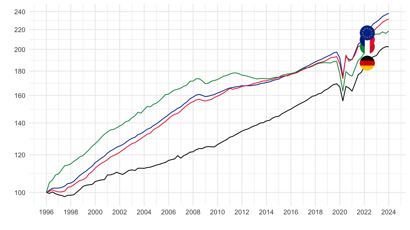
Volume
Code
namq_10_gdp %>%
  filter(geo %in% c("EA19", "DE", "IT", "FR"),
         # B1GQ: Gross domestic product at market prices
         na_item == "P3",
         # SCA: Seasonally and calendar adjusted data
         s_adj == "SCA",
         # CLV10_MEUR: Chain linked volumes (2010), million euro
         unit == "CLV10_MEUR") %>%
  quarter_to_date %>%
  filter(date >= as.Date("1996-01-01")) %>%

  mutate(Geo = ifelse(geo == "EA19", "Europe", Geo)) %>%
  group_by(geo) %>%
  mutate(values = 100*values / values[1]) %>%
  left_join(colors, by = c("Geo" = "country")) %>%
  ggplot + geom_line(aes(x = date, y = values, color = color)) +
  scale_color_identity() + theme_minimal() + xlab("") + ylab("") +
  scale_x_date(breaks = as.Date(paste0(seq(1960, 2100, 2), "-01-01")),
               labels = date_format("%Y")) +
  add_4flags +
  theme(legend.position = c(0.35, 0.85),
        legend.title = element_blank()) +
  scale_y_log10(breaks = seq(100, 400, 5),
                labels = dollar_format(suffix = "", prefix = "", accuracy = 1))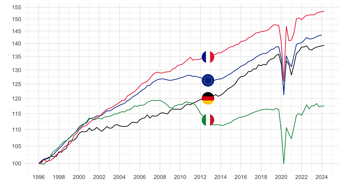
2000-
Code
namq_10_gdp %>%
  filter(geo %in% c("EA19", "DE", "IT", "FR"),
         # B1GQ: Gross domestic product at market prices
         na_item == "P3",
         # SCA: Seasonally and calendar adjusted data
         s_adj == "SCA",
         # CLV10_MEUR: Chain linked volumes (2010), million euro
         unit == "CP_MEUR") %>%
  quarter_to_date %>%
  filter(date >= as.Date("2000-01-01")) %>%

  mutate(Geo = ifelse(geo == "EA19", "Europe", Geo)) %>%
  group_by(geo) %>%
  mutate(values = 100*values / values[date == as.Date("2000-01-01")]) %>%
  left_join(colors, by = c("Geo" = "country")) %>%
  ggplot + geom_line(aes(x = date, y = values, color = color)) +
  scale_color_identity() + theme_minimal() + xlab("") + ylab("") +
  scale_x_date(breaks = as.Date(paste0(seq(1960, 2100, 5), "-01-01")),
               labels = date_format("%Y")) +
  add_4flags +
  theme(legend.position = c(0.35, 0.85),
        legend.title = element_blank()) +
  scale_y_log10(breaks = seq(100, 400, 20),
                labels = dollar_format(suffix = "", prefix = "", accuracy = 1))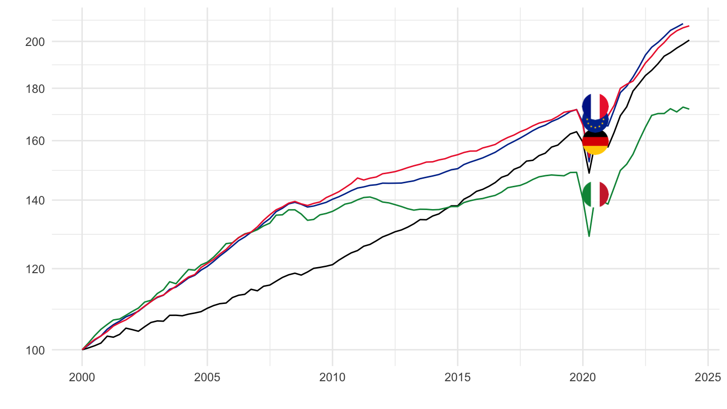
2015-
Code
namq_10_gdp %>%
  filter(geo %in% c("EA19", "DE", "IT", "FR"),
         # B1GQ: Gross domestic product at market prices
         na_item == "P3",
         # SCA: Seasonally and calendar adjusted data
         s_adj == "SCA",
         # CLV10_MEUR: Chain linked volumes (2010), million euro
         unit == "CP_MEUR") %>%
  quarter_to_date %>%
  filter(date >= as.Date("2015-01-01")) %>%

  mutate(Geo = ifelse(geo == "EA19", "Europe", Geo)) %>%
  group_by(geo) %>%
  mutate(values = 100*values / values[date == as.Date("2015-01-01")]) %>%
  left_join(colors, by = c("Geo" = "country")) %>%
  ggplot + geom_line(aes(x = date, y = values, color = color)) +
  scale_color_identity() + theme_minimal() + xlab("") + ylab("") +
  scale_x_date(breaks = as.Date(paste0(seq(1960, 2100, 1), "-01-01")),
               labels = date_format("%Y")) +
  add_4flags +
  theme(legend.position = c(0.35, 0.85),
        legend.title = element_blank()) +
  scale_y_log10(breaks = seq(80, 400, 2),
                labels = dollar_format(suffix = "", prefix = "", accuracy = 1))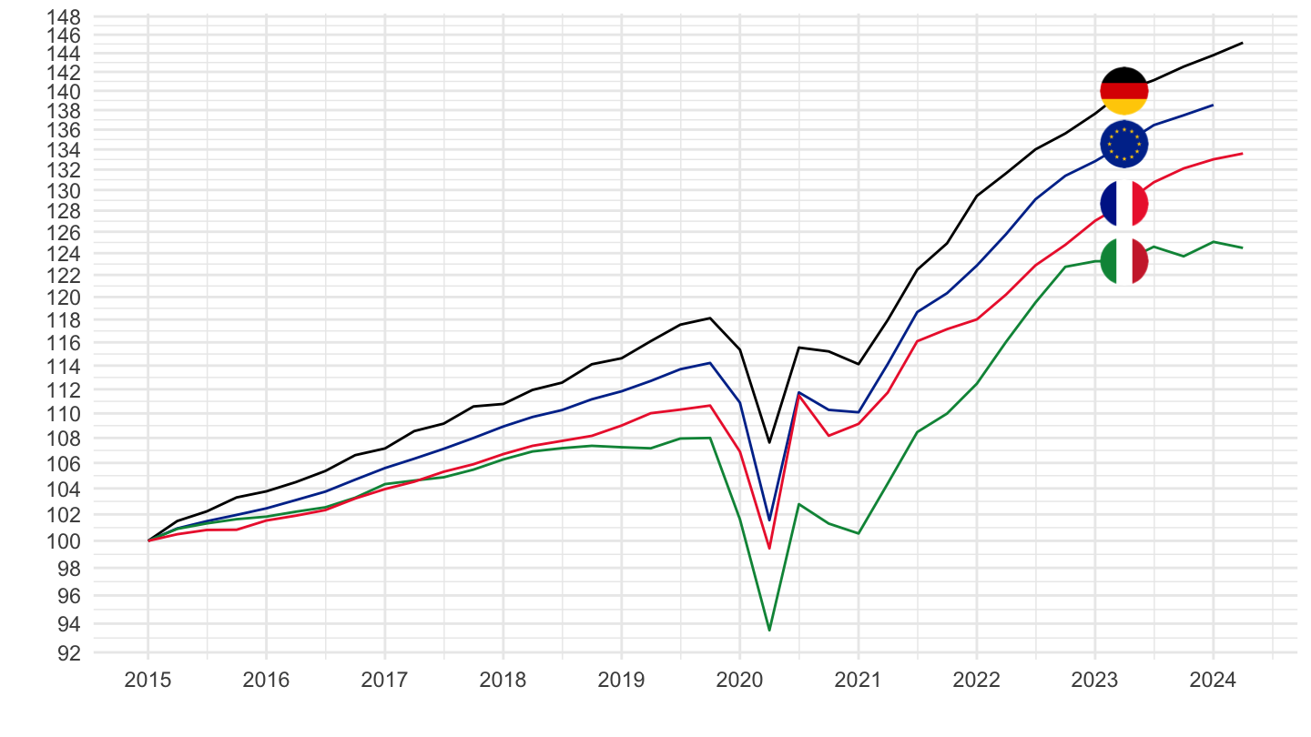
2017-
Code
namq_10_gdp %>%
  filter(geo %in% c("EA19", "DE", "IT", "FR"),
         # B1GQ: Gross domestic product at market prices
         na_item == "P3",
         # SCA: Seasonally and calendar adjusted data
         s_adj == "SCA",
         # CLV10_MEUR: Chain linked volumes (2010), million euro
         unit == "CP_MEUR") %>%
  quarter_to_date %>%
  filter(date >= as.Date("2017-01-01")) %>%

  mutate(Geo = ifelse(geo == "EA19", "Europe", Geo)) %>%
  group_by(geo) %>%
  mutate(values = 100*values / values[date == as.Date("2017-01-01")]) %>%
  left_join(colors, by = c("Geo" = "country")) %>%
  ggplot + geom_line(aes(x = date, y = values, color = color)) +
  scale_color_identity() + theme_minimal() + xlab("") + ylab("") +
  scale_x_date(breaks = as.Date(paste0(seq(1960, 2100, 1), "-01-01")),
               labels = date_format("%Y")) +
  add_4flags +
  theme(legend.position = c(0.35, 0.85),
        legend.title = element_blank()) +
  scale_y_log10(breaks = seq(80, 400, 5),
                labels = dollar_format(suffix = "", prefix = "", accuracy = 1))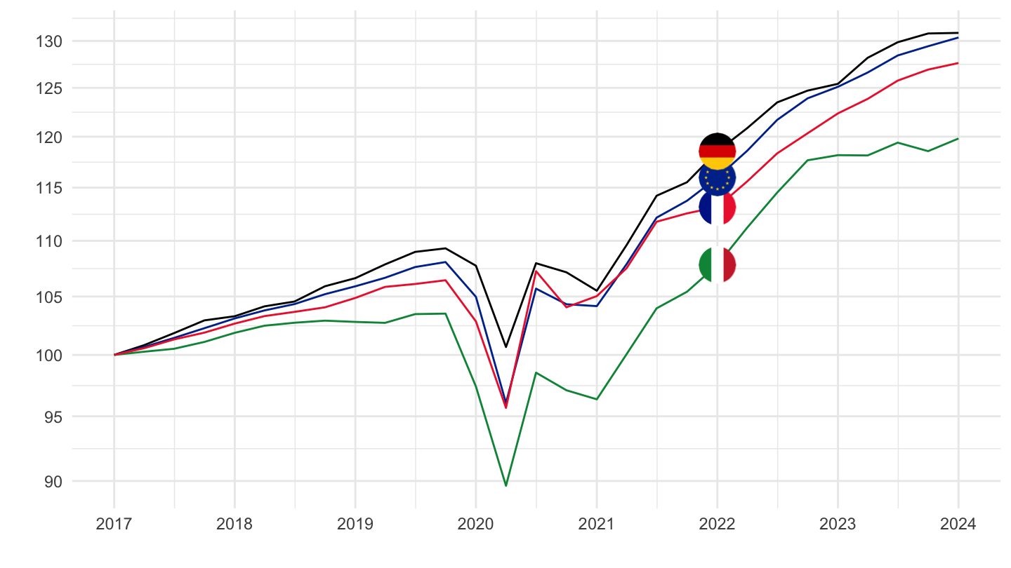
Import Price index
Table
Code
namq_10_gdp %>%
  filter(na_item == "P7",
         unit == "PD15_EUR",
         time %in% c("2022Q1", "2021Q4")) %>%
  spread(time, values) %>%
  select_if(~ n_distinct(.) > 1) %>%
  mutate(`growth` = 100*( `2022Q1`/`2021Q4`-1 )) %>%
  arrange(-`growth`) %>%

  select(geo, Geo, everything()) %>%
  print_table_conditional
Last observation, Eurozone
Code
namq_10_gdp %>%
  filter(time == max(time),
         na_item == "B1GQ") %>%
  spread(unit, values) %>%
  select_if(~ n_distinct(.) > 1) %>%

  select(geo, Geo, everything()) %>%
  print_table_conditional