Production and Sales (MEI)
Data - OECD
François Geerolf
Info
| source | dataset | .html | .RData |
|---|---|---|---|
| oecd | MEI_REAL | 2024-05-06 | 2024-05-03 |
Data on industry
| source | dataset | .html | .RData |
|---|---|---|---|
| ec | INDUSTRY | 2023-10-01 | 2023-10-01 |
| eurostat | ei_isin_m | 2024-05-09 | 2024-05-09 |
| eurostat | htec_trd_group4 | 2024-05-09 | 2024-05-09 |
| eurostat | nama_10_a64 | 2024-05-12 | 2024-05-09 |
| eurostat | nama_10_a64_e | 2024-05-12 | 2024-05-09 |
| eurostat | namq_10_a10_e | 2024-05-09 | 2024-05-09 |
| eurostat | road_eqr_carmot | 2024-05-09 | 2024-05-09 |
| eurostat | sts_inpp_m | 2024-05-09 | 2024-05-09 |
| eurostat | sts_inppd_m | 2024-05-09 | 2024-05-09 |
| eurostat | sts_inpr_m | 2024-05-12 | 2024-05-12 |
| eurostat | sts_intvnd_m | 2024-05-09 | 2024-05-09 |
| fred | industry | 2024-05-10 | 2024-05-10 |
| oecd | ALFS_EMP | 2024-04-16 | 2024-05-12 |
| oecd | BERD_MA_SOF | 2024-04-16 | 2023-09-09 |
| oecd | GBARD_NABS2007 | 2024-04-16 | 2023-11-22 |
| oecd | MEI_REAL | 2024-05-06 | 2024-05-03 |
| oecd | MSTI_PUB | 2024-04-16 | 2023-10-04 |
| oecd | SNA_TABLE4 | 2024-04-30 | 2024-04-30 |
| wdi | NV.IND.EMPL.KD | 2024-01-06 | 2024-04-14 |
| wdi | NV.IND.MANF.CD | 2024-04-14 | 2024-04-14 |
| wdi | NV.IND.MANF.ZS | 2024-01-06 | 2024-04-14 |
| wdi | NV.IND.TOTL.KD | 2024-01-06 | 2024-04-14 |
| wdi | NV.IND.TOTL.ZS | 2024-01-06 | 2024-04-14 |
| wdi | SL.IND.EMPL.ZS | 2024-01-06 | 2024-04-14 |
| wdi | TX.VAL.MRCH.CD.WT | 2024-01-06 | 2024-04-14 |
Data on macro
| source | dataset | .html | .RData |
|---|---|---|---|
| eurostat | nama_10_a10 | 2024-05-09 | 2024-05-09 |
| eurostat | nama_10_a10_e | 2024-05-09 | 2024-05-09 |
| eurostat | nama_10_gdp | 2024-05-09 | 2024-05-09 |
| eurostat | nama_10_lp_ulc | 2024-05-09 | 2024-05-09 |
| eurostat | namq_10_a10 | 2024-05-09 | 2024-05-09 |
| eurostat | namq_10_a10_e | 2024-05-09 | 2024-05-09 |
| eurostat | namq_10_gdp | 2024-05-10 | 2024-05-09 |
| eurostat | namq_10_lp_ulc | 2024-05-09 | 2024-05-09 |
| eurostat | namq_10_pc | 2024-05-09 | 2024-05-09 |
| eurostat | nasa_10_nf_tr | 2024-05-09 | 2024-05-09 |
| eurostat | nasq_10_nf_tr | 2024-05-11 | 2024-05-09 |
| fred | gdp | 2024-05-10 | 2024-05-10 |
| oecd | QNA | 2024-05-05 | 2024-04-15 |
| oecd | SNA_TABLE1 | 2024-04-16 | 2024-04-15 |
| oecd | SNA_TABLE14A | 2024-04-16 | 2024-04-15 |
| oecd | SNA_TABLE2 | 2024-04-16 | 2024-04-11 |
| oecd | SNA_TABLE6A | 2024-04-30 | 2024-04-15 |
| wdi | NE.RSB.GNFS.ZS | 2024-04-14 | 2024-04-14 |
| wdi | NY.GDP.MKTP.CD | 2024-04-25 | 2024-05-06 |
| wdi | NY.GDP.MKTP.PP.CD | 2024-04-14 | 2024-04-14 |
| wdi | NY.GDP.PCAP.CD | 2024-04-14 | 2024-04-22 |
| wdi | NY.GDP.PCAP.KD | 2024-04-14 | 2024-05-06 |
| wdi | NY.GDP.PCAP.PP.CD | 2024-04-24 | 2024-04-22 |
| wdi | NY.GDP.PCAP.PP.KD | 2024-05-06 | 2024-05-06 |
Last
| obsTime | FREQUENCY | Nobs |
|---|---|---|
| 2023-Q4 | Q | 9 |
| 2023-12 | M | 15 |
| 2023 | A | 11 |
Nobs - Javascript
MEI_REAL %>%
  left_join(MEI_REAL_var$SUBJECT, by = c("SUBJECT")) %>%
  {if (!is_html_output()) mutate(., Subject = substr(Subject, 1, 87)) else .} %>%
  group_by(SUBJECT, Subject, FREQUENCY) %>%
  filter(!is.na(obsValue)) %>%
  summarise(Nobs = n()) %>%
  arrange(-Nobs) %>%
  {if (is_html_output()) datatable(., filter = 'top', rownames = F) else .}
SUBJECT
MEI_REAL %>%
  left_join(MEI_REAL_var$SUBJECT, by = c("SUBJECT")) %>%
  group_by(SUBJECT, Subject) %>%
  summarise(Nobs = n()) %>%
  arrange(-Nobs) %>%
print_table_conditional()| SUBJECT | Subject | Nobs |
|---|---|---|
| PRINTO01 | Production of total industry sa, Index | 38594 |
| PRMNTO01 | Production in total manufacturing sa, Index | 36515 |
| SLRTTO01 | Total retail trade (Volume) sa, Index | 30670 |
| PRCNTO01 | Production of total construction sa, Index | 20762 |
| SLRTCR03 | Passenger car registrations sa, Index | 20344 |
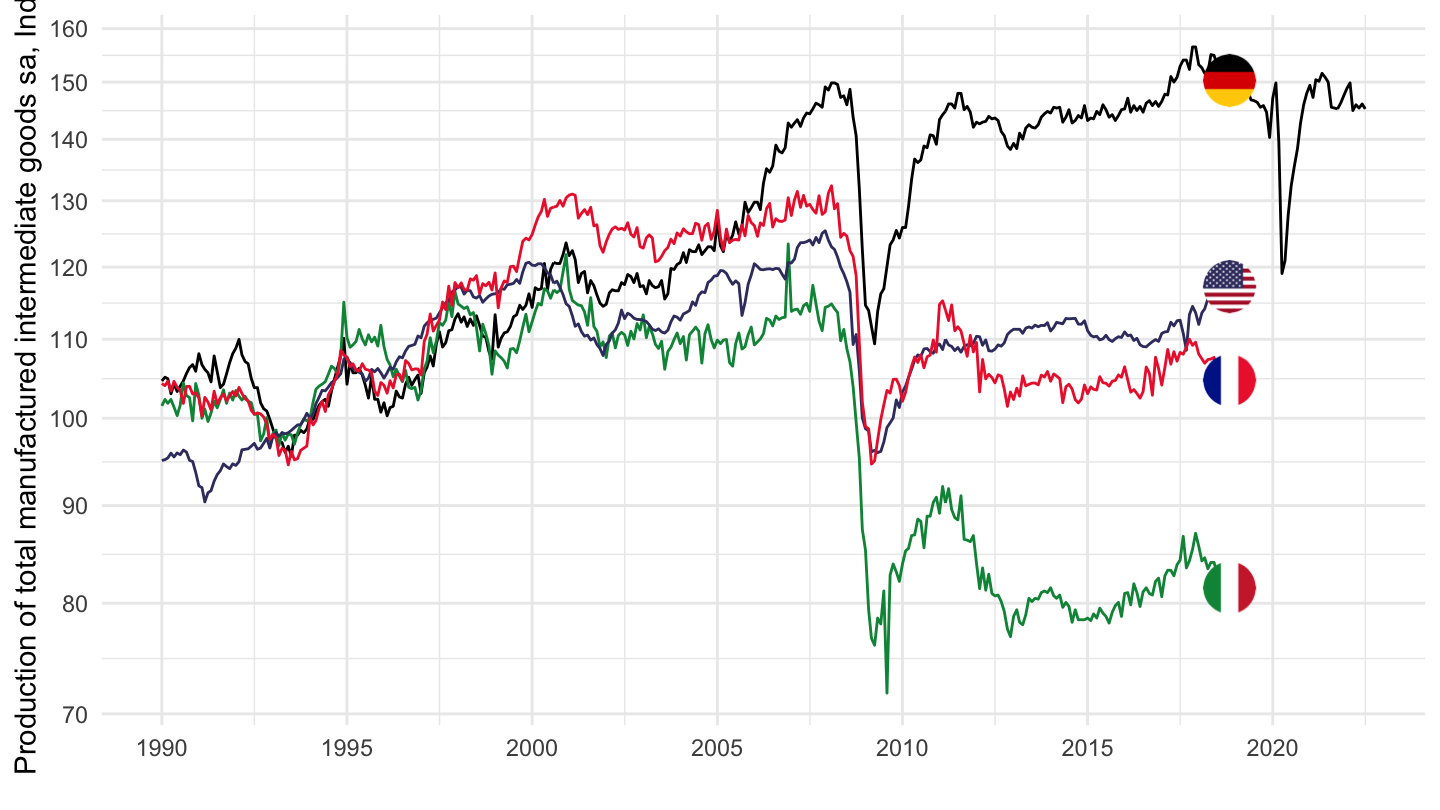
| PRMNIG01 | Production of total manufactured intermediate goods sa, Index | 19883 |
| PRMNVG01 | Production of total manufactured investment goods sa, Index | 19228 |
| ODCNPI03 | Permits issued for dwellings sa, Index | 16770 |
| PREND401 | Production of electricity, gas, steam and air conditioning supply sa, index | 13863 |
| WSCNDW01 | Work started for dwellings sa, Index | 8159 |
| PRENTO01 | Production of total energy sa, Index | 2906 |
LOCATION
MEI_REAL %>%
  left_join(MEI_REAL_var$LOCATION, by = "LOCATION") %>%
  group_by(LOCATION, Location) %>%
  summarise(Nobs = n()) %>%
  arrange(-Nobs) %>%
  mutate(Flag = gsub(" ", "-", str_to_lower(gsub(" ", "-", Location))),
         Flag = paste0('<img src="../../icon/flag/vsmall/', Flag, '.png" alt="Flag">')) %>%
  select(Flag, everything()) %>%
  {if (is_html_output()) datatable(., filter = 'top', rownames = F, escape = F) else .}
FREQUENCY
MEI_REAL %>%
  left_join(MEI_REAL_var$FREQUENCY, by = c("FREQUENCY")) %>%
  group_by(FREQUENCY, Frequency) %>%
  summarise(Nobs = n()) %>%
  arrange(-Nobs) %>%
print_table_conditional()| FREQUENCY | Frequency | Nobs |
|---|---|---|
| M | Monthly | 163229 |
| Q | Quarterly | 51415 |
| A | Annual | 13050 |
obsTime
Passenger car registrations - SLRTCR0
All Countries
MEI_REAL %>%
  left_join(MEI_REAL_var$LOCATION, by = "LOCATION") %>%
  filter(SUBJECT == "SLRTCR03") %>%
  group_by(LOCATION, Location, FREQUENCY) %>%
  arrange(obsTime) %>%
  summarise(Nobs = n(),
            obsTime1 = first(obsTime),
            obsTime2 = last(obsTime)) %>%
  arrange(-Nobs) %>%
  mutate(Flag = gsub(" ", "-", str_to_lower(gsub(" ", "-", Location))),
         Flag = paste0('<img src="../../icon/flag/vsmall/', Flag, '.png" alt="Flag">')) %>%
  select(Flag, everything()) %>%
  {if (is_html_output()) datatable(., filter = 'top', rownames = F, escape = F) else .}
France, Germany, Italy, United States
Monthly
MEI_REAL %>%
  left_join(MEI_REAL_var$LOCATION, by = "LOCATION") %>%
  filter(SUBJECT == "SLRTCR03",
         FREQUENCY == "M",
         LOCATION %in% c("FRA", "DEU", "ITA", "USA")) %>%
  month_to_date %>%
  left_join(colors, by = c("Location" = "country")) %>%
  ggplot(.) + geom_line(aes(x = date, y = obsValue, color = color)) +
  scale_color_identity() + add_3flags +
  theme_minimal() + xlab("") + ylab("Passenger car registrations") +
  scale_x_date(breaks = seq(1950, 2100, 5) %>% paste0("-01-01") %>% as.Date,
               labels = date_format("%Y")) +
  scale_y_log10(breaks = seq(-10, 300, 10),
                     labels = dollar_format(accuracy = 1, prefix = "")) +
  theme(legend.position = c(0.2, 0.80),
        legend.title = element_blank())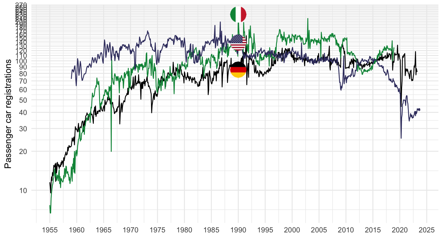
Production in total manuf. na., Index - PRMNTO01, PRINTO01
France
MEI_REAL %>%
  left_join(MEI_REAL_var$SUBJECT, by = "SUBJECT") %>%
  filter(SUBJECT %in% c("PRMNTO01", "PRINTO01"),
         FREQUENCY == "M",
         LOCATION %in% c("FRA")) %>%
  month_to_date %>%
  filter(date >= as.Date("1990-01-01")) %>%
  group_by(Subject) %>%
  mutate(obsValue = 100*obsValue/obsValue[date == as.Date("2001-01-01")]) %>%
  ggplot(.) + geom_line(aes(x = date, y = obsValue, color = Subject)) +
  #scale_color_identity() +
  theme_minimal() + xlab("") + ylab("") +
  scale_x_date(breaks = seq(1910, 2100, 5) %>% paste0("-01-01") %>% as.Date,
               labels = date_format("%Y")) +
  scale_y_log10(breaks = seq(-10, 300, 10),
                     labels = dollar_format(accuracy = 1, prefix = "")) +
  theme(legend.position = c(0.2, 0.80),
        legend.title = element_blank())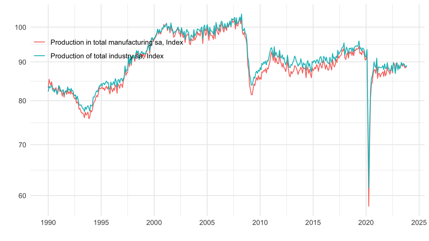
Production in total manufacturing sa, Index - PRMNTO01
Table
MEI_REAL %>%
  left_join(MEI_REAL_var$LOCATION, by = "LOCATION") %>%
  filter(SUBJECT == "PRMNTO01") %>%
  group_by(LOCATION, Location, FREQUENCY) %>%
  summarise(Nobs = n(),
            obsTime1 = first(obsTime),
            obsTime2 = last(obsTime)) %>%
  arrange(-Nobs) %>%
  mutate(Flag = gsub(" ", "-", str_to_lower(gsub(" ", "-", Location))),
         Flag = paste0('<img src="../../icon/flag/vsmall/', Flag, '.png" alt="Flag">')) %>%
  select(Flag, everything()) %>%
  {if (is_html_output()) datatable(., filter = 'top', rownames = F, escape = F) else .}
Euro Area, United States
1999-
plot <- MEI_REAL %>%
  left_join(MEI_REAL_var$LOCATION, by = "LOCATION") %>%
  filter(SUBJECT == "PRMNTO01",
         FREQUENCY == "M",
         LOCATION %in% c("USA", "EA20")) %>%
  month_to_date %>%
  filter(date >= as.Date("1999-01-01")) %>%
  group_by(Location) %>%
  mutate(obsValue = 100*obsValue/obsValue[date == as.Date("1999-01-01")]) %>%
  mutate(Location = ifelse(LOCATION == "EA20", "Europe", Location)) %>%
  left_join(colors, by = c("Location" = "country")) %>%
  mutate(color = ifelse(LOCATION == "USA", color2, color)) %>%
  ggplot(.) + geom_line(aes(x = date, y = obsValue, color = color)) +
  scale_color_identity() + add_2flags +
  theme_minimal() + xlab("") + ylab("Production manufacturière (Janv. 1999 = 100)") +
  scale_x_date(breaks = c(seq(1999, 2100, 5),seq(1997, 2100, 5)) %>% paste0("-01-01") %>% as.Date,
               labels = date_format("%Y")) +
  scale_y_log10(breaks = seq(-10, 300, 5),
                     labels = dollar_format(accuracy = 1, prefix = "")) +
  theme(legend.position = c(0.2, 0.80),
        legend.title = element_blank()) +
  geom_rect(data = nber_recessions %>%
              filter(Peak > as.Date("1999-01-01")),
            aes(xmin = Peak, xmax = Trough, ymin = 0, ymax = +Inf),
            fill = '#B22234', alpha = 0.1)  +
  geom_rect(data = cepr_recessions %>%
              filter(Peak > as.Date("1999-01-01")),
            aes(xmin = Peak, xmax = Trough, ymin = 0, ymax = +Inf),
            fill = '#003399', alpha = 0.1)

save(plot, file = "MEI_REAL_files/figure-html/PRMNTO01-USA-EA20-1999-1.RData")
plot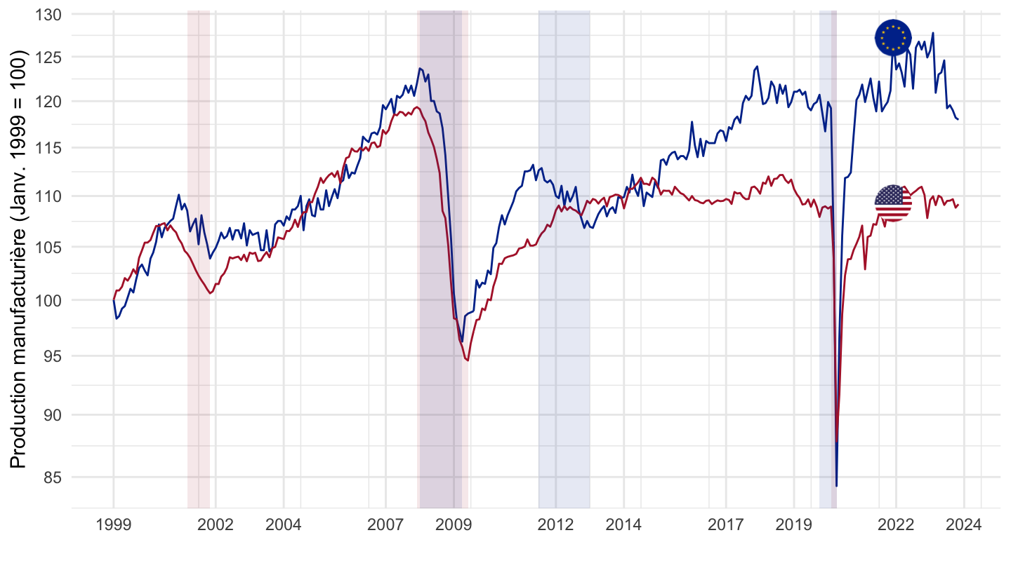
France, Germany
Monthly
All
MEI_REAL %>%
  left_join(MEI_REAL_var$LOCATION, by = "LOCATION") %>%
  filter(SUBJECT == "PRMNTO01",
         FREQUENCY == "M",
         LOCATION %in% c("FRA", "DEU")) %>%
  month_to_date %>%
  left_join(colors, by = c("Location" = "country")) %>%
  ggplot(.) + geom_line(aes(x = date, y = obsValue, color = color)) +
  scale_color_identity() + add_2flags +
  theme_minimal() + xlab("") + ylab("Passenger car registrations") +
  scale_x_date(breaks = seq(1910, 2100, 5) %>% paste0("-01-01") %>% as.Date,
               labels = date_format("%Y")) +
  scale_y_log10(breaks = seq(-10, 300, 10),
                     labels = dollar_format(accuracy = 1, prefix = ""))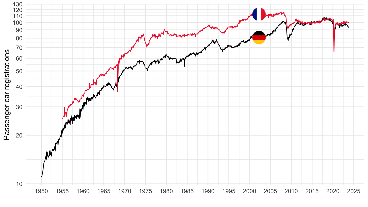
1980-
MEI_REAL %>%
  left_join(MEI_REAL_var$LOCATION, by = "LOCATION") %>%
  filter(SUBJECT == "PRMNTO01",
         FREQUENCY == "M",
         LOCATION %in% c("FRA", "DEU")) %>%
  month_to_date %>%
  filter(date >= as.Date("1980-01-01")) %>%
  group_by(LOCATION) %>%
  mutate(obsValue = 100*obsValue/obsValue[date == as.Date("1980-01-01")]) %>%
  left_join(colors, by = c("Location" = "country")) %>%
  ggplot(.) + geom_line(aes(x = date, y = obsValue, color = color)) +
  scale_color_identity() + add_2flags +
  theme_minimal() + xlab("") + ylab("Production in total manufacturing") +
  scale_x_date(breaks = seq(1910, 2100, 5) %>% paste0("-01-01") %>% as.Date,
               labels = date_format("%Y")) +
  scale_y_log10(breaks = seq(-10, 300, 10),
                     labels = dollar_format(accuracy = 1, prefix = ""))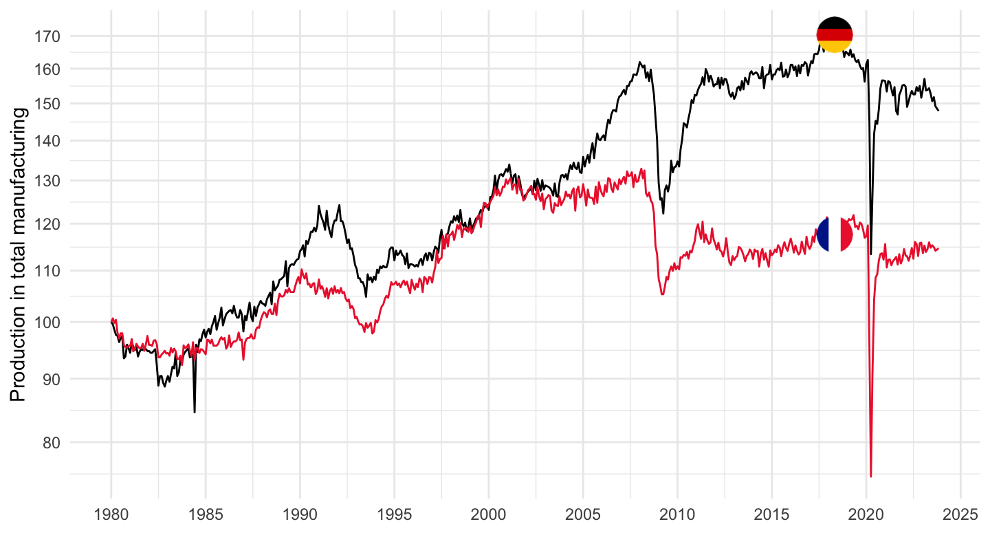
1995-
MEI_REAL %>%
  left_join(MEI_REAL_var$LOCATION, by = "LOCATION") %>%
  filter(SUBJECT == "PRMNTO01",
         FREQUENCY == "M",
         LOCATION %in% c("FRA", "DEU")) %>%
  month_to_date %>%
  filter(date >= as.Date("1995-01-01")) %>%
  group_by(LOCATION) %>%
  mutate(obsValue = 100*obsValue/obsValue[date == as.Date("1995-01-01")]) %>%
  left_join(colors, by = c("Location" = "country")) %>%
  ggplot(.) + geom_line(aes(x = date, y = obsValue, color = color)) +
  scale_color_identity() + add_2flags +
  theme_minimal() + xlab("") + ylab("Production in total manufacturing") +
  scale_x_date(breaks = seq(1910, 2025, 5) %>% paste0("-01-01") %>% as.Date,
               labels = date_format("%Y")) +
  scale_y_log10(breaks = seq(-10, 300, 10),
                     labels = dollar_format(accuracy = 1, prefix = ""))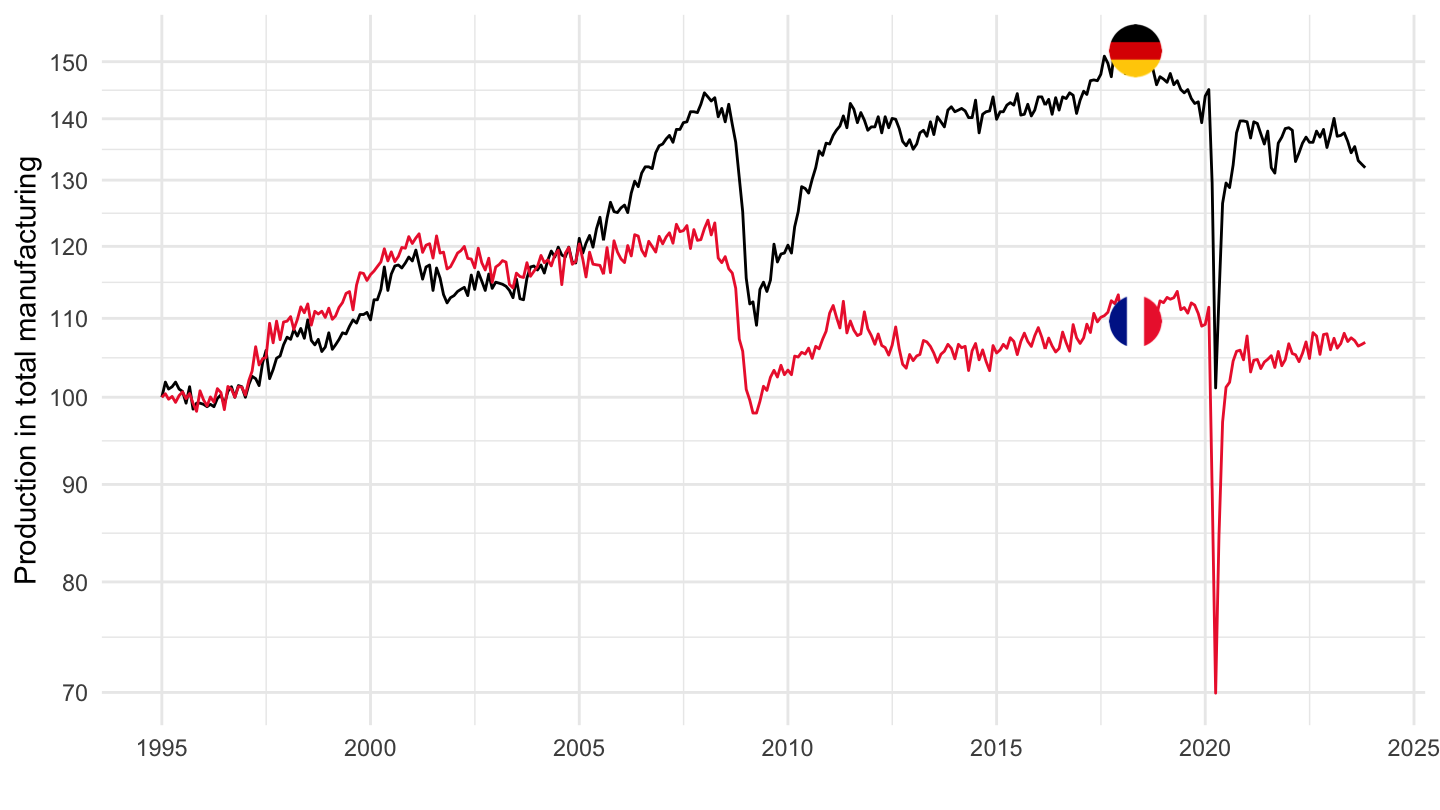
2000-
MEI_REAL %>%
  left_join(MEI_REAL_var$LOCATION, by = "LOCATION") %>%
  filter(SUBJECT == "PRMNTO01",
         FREQUENCY == "M",
         LOCATION %in% c("FRA", "DEU")) %>%
  month_to_date %>%
  filter(date >= as.Date("2000-01-01")) %>%
  group_by(LOCATION) %>%
  mutate(obsValue = 100*obsValue/obsValue[date == as.Date("2000-01-01")]) %>%
  left_join(colors, by = c("Location" = "country")) %>%
  ggplot(.) + geom_line(aes(x = date, y = obsValue, color = color)) +
  scale_color_identity() + add_2flags +
  theme_minimal() + xlab("") + ylab("Production in total manufacturing") +
  scale_x_date(breaks = seq(1910, 2100, 2) %>% paste0("-01-01") %>% as.Date,
               labels = date_format("%Y")) +
  scale_y_log10(breaks = seq(-10, 300, 10),
                     labels = dollar_format(accuracy = 1, prefix = ""))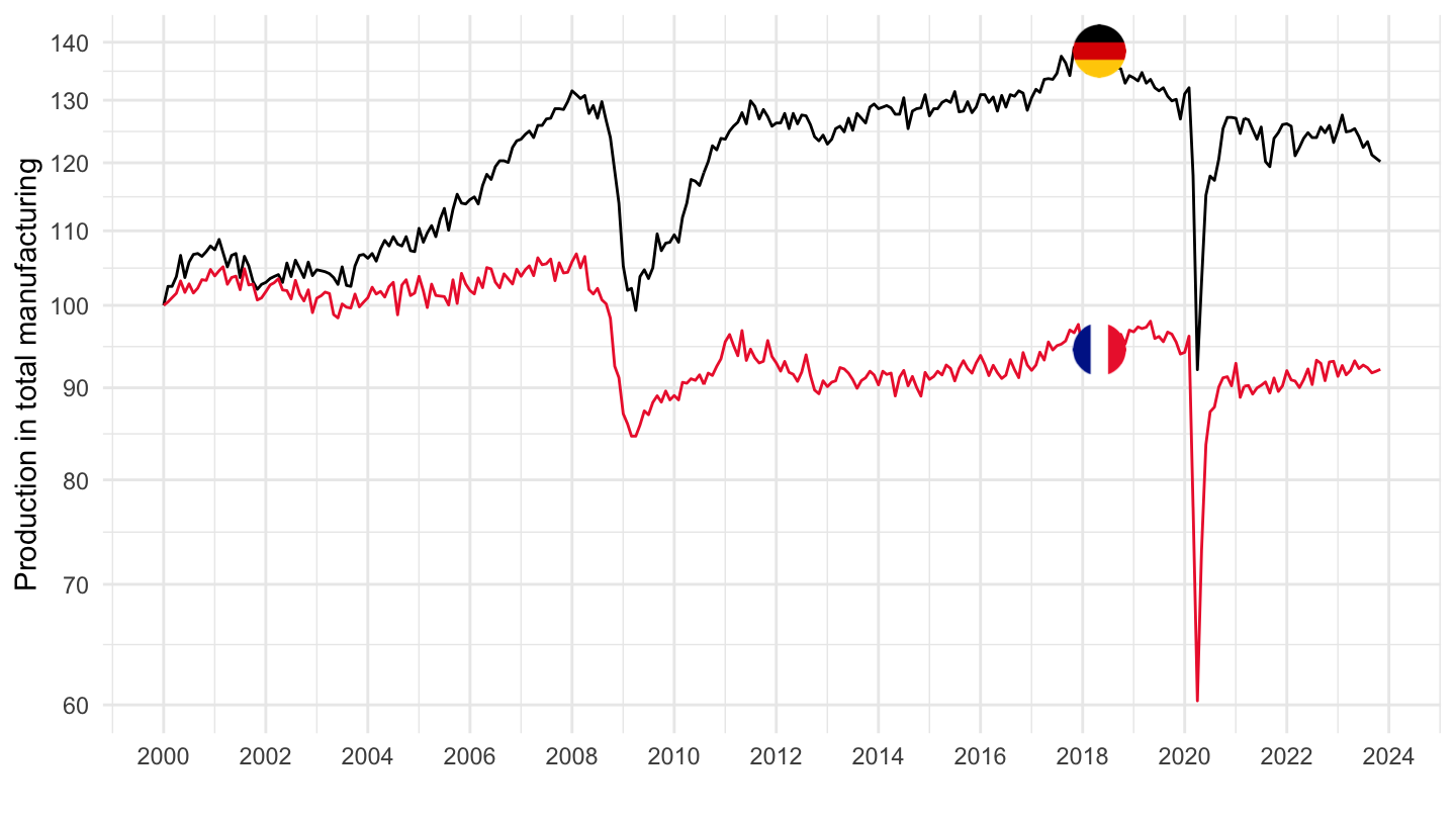
United States, Euro Area, Germany, United Kingdom
Monthly
1995-
MEI_REAL %>%
  left_join(MEI_REAL_var$LOCATION, by = "LOCATION") %>%
  filter(SUBJECT == "PRMNTO01",
         FREQUENCY == "M",
         LOCATION %in% c("FRA", "DEU", "GBR", "USA", "EA20")) %>%
  month_to_date %>%
  filter(date >= as.Date("1995-01-01")) %>%
  group_by(Location) %>%
  mutate(obsValue = 100*obsValue/obsValue[date == as.Date("1995-01-01")]) %>%
  mutate(Location = ifelse(LOCATION == "EA20", "Europe", Location)) %>%
  left_join(colors, by = c("Location" = "country")) %>%
  mutate(color = ifelse(LOCATION == "USA", color2, color)) %>%
  ggplot(.) + geom_line(aes(x = date, y = obsValue, color = color)) +
  scale_color_identity() + add_5flags +
  theme_minimal() + xlab("") + ylab("Production in total manufacturing sa") +
  scale_x_date(breaks = seq(1910, 2100, 5) %>% paste0("-01-01") %>% as.Date,
               labels = date_format("%Y")) +
  scale_y_log10(breaks = seq(-10, 300, 10),
                     labels = dollar_format(accuracy = 1, prefix = "")) +
  theme(legend.position = c(0.2, 0.80),
        legend.title = element_blank())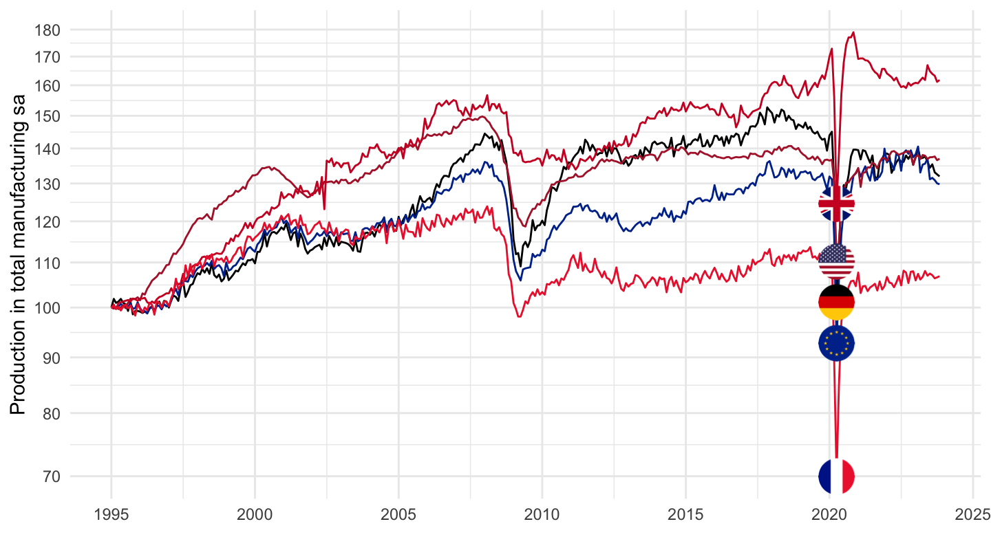
2000-
MEI_REAL %>%
  left_join(MEI_REAL_var$LOCATION, by = "LOCATION") %>%
  filter(SUBJECT == "PRMNTO01",
         FREQUENCY == "M",
         LOCATION %in% c("FRA", "DEU", "GBR", "USA", "EA20")) %>%
  month_to_date %>%
  filter(date >= as.Date("2000-01-01")) %>%
  group_by(Location) %>%
  mutate(obsValue = 100*obsValue/obsValue[date == as.Date("2000-01-01")]) %>%
  mutate(Location = ifelse(LOCATION == "EA20", "Europe", Location)) %>%
  left_join(colors, by = c("Location" = "country")) %>%
  mutate(color = ifelse(LOCATION == "USA", color2, color)) %>%
  ggplot(.) + geom_line(aes(x = date, y = obsValue, color = color)) +
  scale_color_identity() + add_5flags +
  theme_minimal() + xlab("") + ylab("Production in total manufacturing sa") +
  scale_x_date(breaks = seq(1910, 2100, 5) %>% paste0("-01-01") %>% as.Date,
               labels = date_format("%Y")) +
  scale_y_log10(breaks = seq(-10, 300, 10),
                     labels = dollar_format(accuracy = 1, prefix = "")) +
  theme(legend.position = c(0.2, 0.80),
        legend.title = element_blank())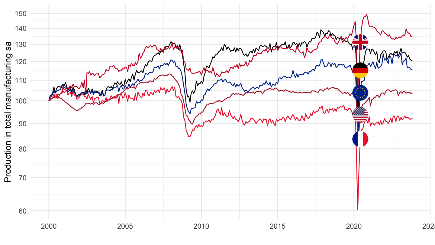
United States, Euro Area, France, Germany
1999-
MEI_REAL %>%
  left_join(MEI_REAL_var$LOCATION, by = "LOCATION") %>%
  filter(SUBJECT == "PRMNTO01",
         FREQUENCY == "M",
         LOCATION %in% c("FRA", "DEU", "USA", "EA20")) %>%
  month_to_date %>%
  filter(date >= as.Date("1999-01-01")) %>%
  group_by(Location) %>%
  mutate(obsValue = 100*obsValue/obsValue[date == as.Date("1999-01-01")]) %>%
  mutate(Location = ifelse(LOCATION == "EA20", "Europe", Location)) %>%
  left_join(colors, by = c("Location" = "country")) %>%
  mutate(color = ifelse(LOCATION == "EA20", color2, color)) %>%
  ggplot(.) + geom_line(aes(x = date, y = obsValue, color = color)) +
  scale_color_identity() + add_4flags +
  theme_minimal() + xlab("") + ylab("Production in total manufacturing sa") +
  scale_x_date(breaks = seq(1999, 2100, 2) %>% paste0("-01-01") %>% as.Date,
               labels = date_format("%Y")) +
  scale_y_log10(breaks = seq(-10, 300, 10),
                     labels = dollar_format(accuracy = 1, prefix = "")) +
  theme(legend.position = c(0.2, 0.80),
        legend.title = element_blank())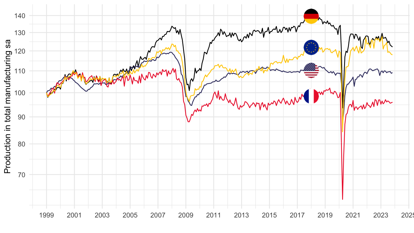
United States, Euro Area, France, Germany, Italy
Monthly
1990-
MEI_REAL %>%
  left_join(MEI_REAL_var$LOCATION, by = "LOCATION") %>%
  filter(SUBJECT == "PRMNTO01",
         FREQUENCY == "M",
         LOCATION %in% c("FRA", "DEU", "ITA", "USA", "EA20")) %>%
  month_to_date %>%
  filter(date >= as.Date("1990-01-01")) %>%
  group_by(Location) %>%
  mutate(obsValue = 100*obsValue/obsValue[date == as.Date("1990-01-01")]) %>%
  mutate(Location = ifelse(LOCATION == "EA20", "Europe", Location)) %>%
  left_join(colors, by = c("Location" = "country")) %>%
  mutate(color = ifelse(LOCATION == "USA", color2, color)) %>%
  ggplot(.) + geom_line(aes(x = date, y = obsValue, color = color)) +
  scale_color_identity() + add_5flags +
  theme_minimal() + xlab("") + ylab("Production in total manufacturing sa") +
  scale_x_date(breaks = seq(1910, 2100, 5) %>% paste0("-01-01") %>% as.Date,
               labels = date_format("%Y")) +
  scale_y_log10(breaks = seq(-10, 300, 10),
                     labels = dollar_format(accuracy = 1, prefix = "")) +
  theme(legend.position = c(0.2, 0.80),
        legend.title = element_blank())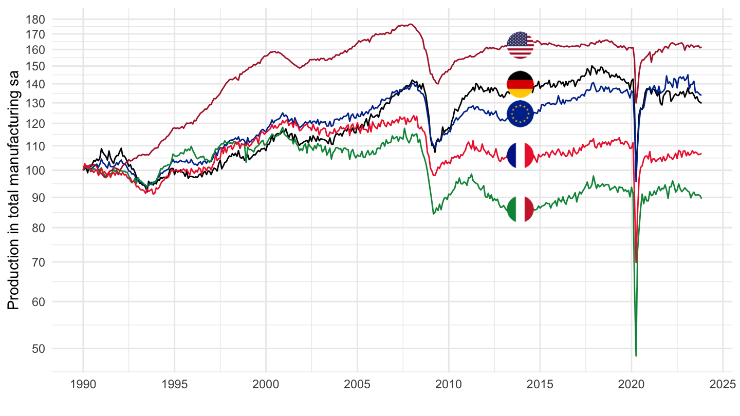
1995-
MEI_REAL %>%
  left_join(MEI_REAL_var$LOCATION, by = "LOCATION") %>%
  filter(SUBJECT == "PRMNTO01",
         FREQUENCY == "M",
         LOCATION %in% c("FRA", "DEU", "ITA", "USA", "EA20")) %>%
  month_to_date %>%
  filter(date >= as.Date("1995-01-01")) %>%
  group_by(Location) %>%
  mutate(obsValue = 100*obsValue/obsValue[date == as.Date("1995-01-01")]) %>%
  mutate(Location = ifelse(LOCATION == "EA20", "Europe", Location)) %>%
  left_join(colors, by = c("Location" = "country")) %>%
  mutate(color = ifelse(LOCATION == "USA", color2, color)) %>%
  ggplot(.) + geom_line(aes(x = date, y = obsValue, color = color)) +
  scale_color_identity() + add_5flags +
  theme_minimal() + xlab("") + ylab("Production in total manufacturing sa") +
  scale_x_date(breaks = seq(1910, 2100, 5) %>% paste0("-01-01") %>% as.Date,
               labels = date_format("%Y")) +
  scale_y_log10(breaks = seq(-10, 300, 10),
                     labels = dollar_format(accuracy = 1, prefix = "")) +
  theme(legend.position = c(0.2, 0.80),
        legend.title = element_blank())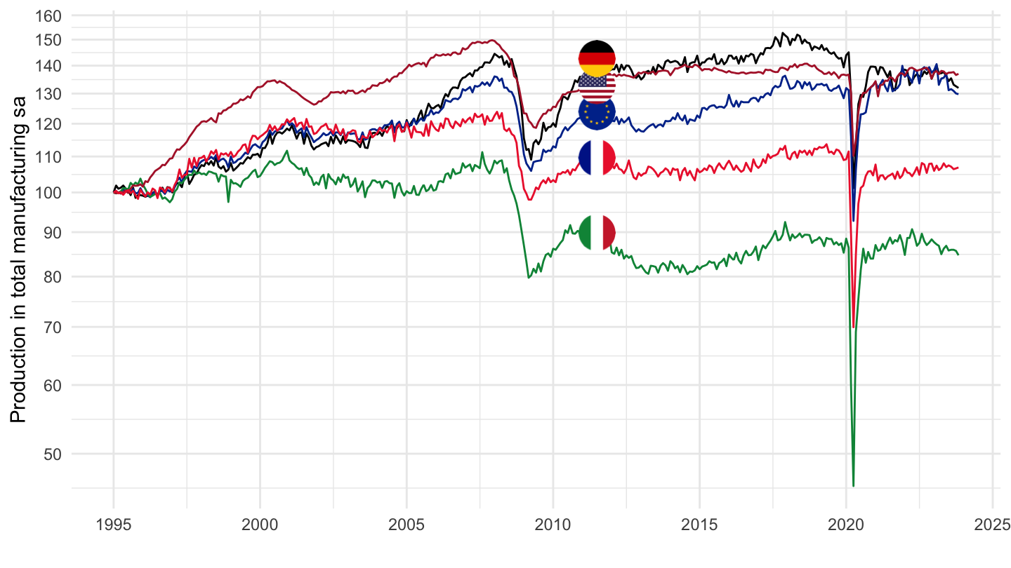
1999-
MEI_REAL %>%
  left_join(MEI_REAL_var$LOCATION, by = "LOCATION") %>%
  filter(SUBJECT == "PRMNTO01",
         FREQUENCY == "M",
         LOCATION %in% c("FRA", "DEU", "ITA", "USA", "EA20")) %>%
  month_to_date %>%
  filter(date >= as.Date("1999-01-01")) %>%
  group_by(Location) %>%
  mutate(obsValue = 100*obsValue/obsValue[date == as.Date("1999-01-01")]) %>%
  mutate(Location = ifelse(LOCATION == "EA20", "Europe", Location)) %>%
  left_join(colors, by = c("Location" = "country")) %>%
  mutate(color = ifelse(LOCATION == "USA", color2, color)) %>%
  ggplot(.) + geom_line(aes(x = date, y = obsValue, color = color)) +
  scale_color_identity() + add_5flags +
  theme_minimal() + xlab("") + ylab("Production in total manufacturing sa") +
  scale_x_date(breaks = seq(1999, 2100, 2) %>% paste0("-01-01") %>% as.Date,
               labels = date_format("%Y")) +
  scale_y_log10(breaks = seq(-10, 300, 10),
                     labels = dollar_format(accuracy = 1, prefix = "")) +
  theme(legend.position = c(0.2, 0.80),
        legend.title = element_blank())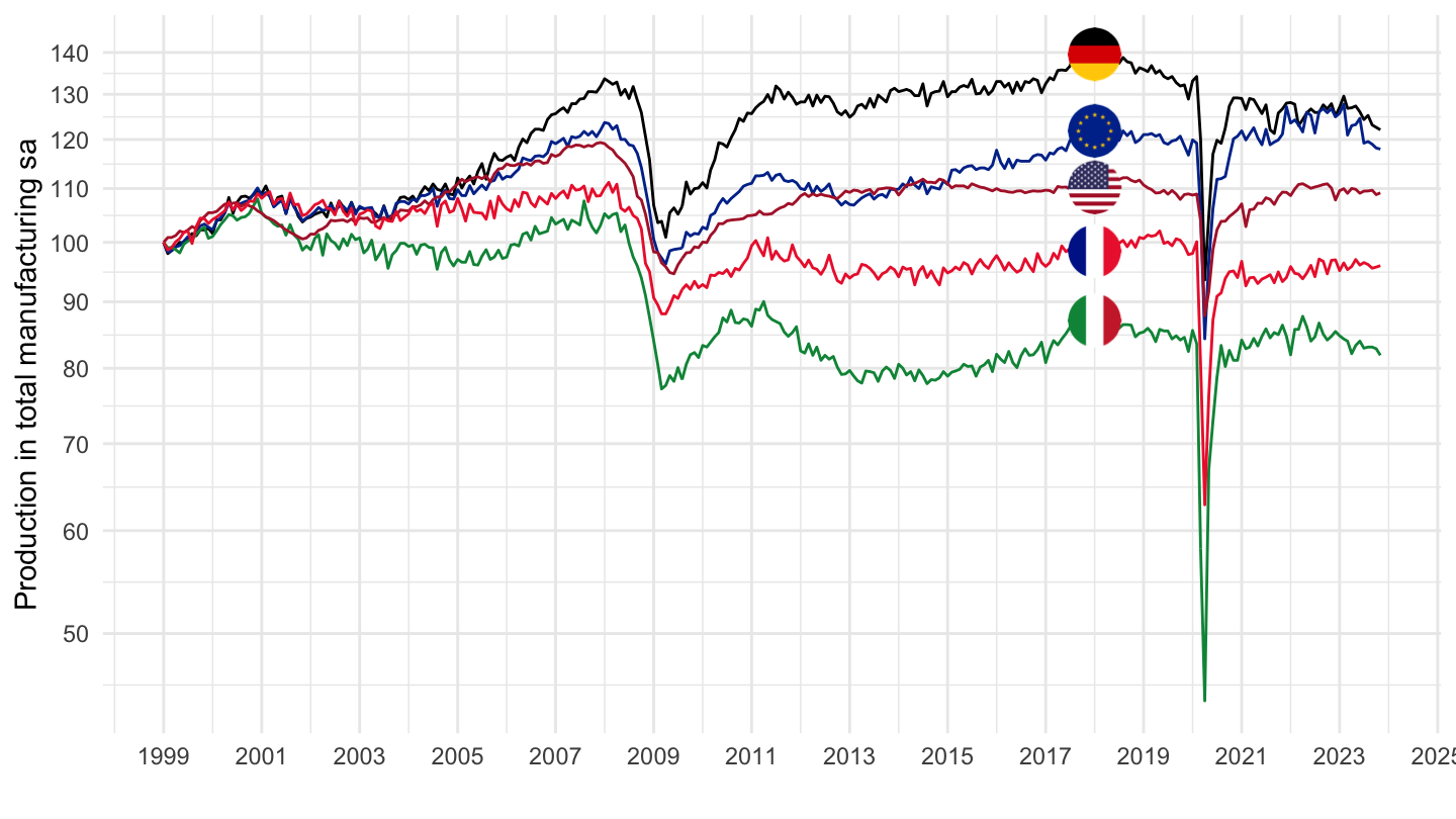
2002-
MEI_REAL %>%
  left_join(MEI_REAL_var$LOCATION, by = "LOCATION") %>%
  filter(SUBJECT == "PRMNTO01",
         FREQUENCY == "M",
         LOCATION %in% c("FRA", "DEU", "ITA", "USA", "EA20")) %>%
  month_to_date %>%
  filter(date >= as.Date("2002-01-01")) %>%
  group_by(Location) %>%
  mutate(obsValue = 100*obsValue/obsValue[date == as.Date("2002-01-01")]) %>%
  mutate(Location = ifelse(LOCATION == "EA20", "Europe", Location)) %>%
  left_join(colors, by = c("Location" = "country")) %>%
  mutate(color = ifelse(LOCATION == "USA", color2, color)) %>%
  ggplot(.) + geom_line(aes(x = date, y = obsValue, color = color)) +
  scale_color_identity() + add_5flags +
  theme_minimal() + xlab("") + ylab("Production in total manufacturing sa") +
  scale_x_date(breaks = seq(1910, 2100, 2) %>% paste0("-01-01") %>% as.Date,
               labels = date_format("%Y")) +
  scale_y_log10(breaks = seq(-10, 300, 10),
                     labels = dollar_format(accuracy = 1, prefix = "")) +
  theme(legend.position = c(0.2, 0.80),
        legend.title = element_blank())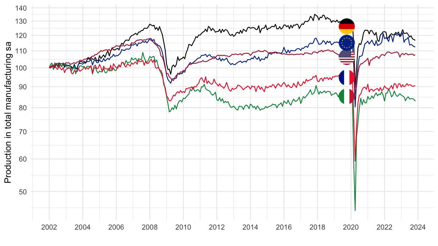
2017-
MEI_REAL %>%
  left_join(MEI_REAL_var$LOCATION, by = "LOCATION") %>%
  filter(SUBJECT == "PRMNTO01",
         FREQUENCY == "M",
         LOCATION %in% c("FRA", "DEU", "ITA", "USA", "EA20")) %>%
  month_to_date %>%
  filter(date >= as.Date("2017-01-01")) %>%
  group_by(Location) %>%
  mutate(obsValue = 100*obsValue/obsValue[date == as.Date("2017-01-01")]) %>%
  mutate(Location = ifelse(LOCATION == "EA20", "Europe", Location)) %>%
  left_join(colors, by = c("Location" = "country")) %>%
  mutate(color = ifelse(LOCATION == "USA", color2, color)) %>%
  ggplot(.) + geom_line(aes(x = date, y = obsValue, color = color)) +
  scale_color_identity() + add_5flags +
  theme_minimal() + xlab("") + ylab("Production in total manufacturing sa") +
  scale_x_date(breaks = seq(1910, 2100, 1) %>% paste0("-01-01") %>% as.Date,
               labels = date_format("%Y")) +
  scale_y_log10(breaks = seq(-10, 300, 10),
                     labels = dollar_format(accuracy = 1, prefix = "")) +
  theme(legend.position = c(0.2, 0.80),
        legend.title = element_blank())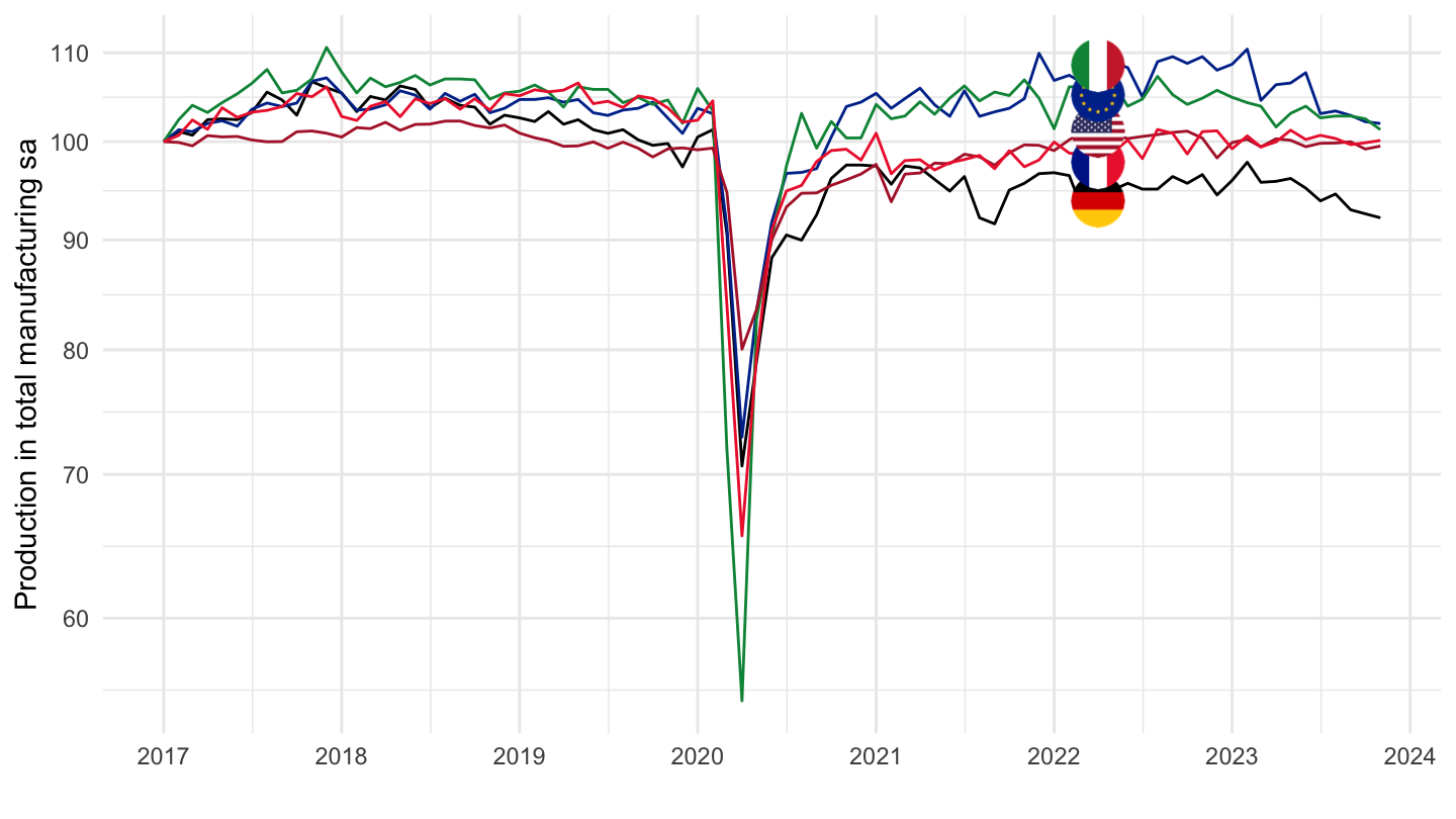
2020-
MEI_REAL %>%
  left_join(MEI_REAL_var$LOCATION, by = "LOCATION") %>%
  filter(SUBJECT == "PRMNTO01",
         FREQUENCY == "M",
         LOCATION %in% c("FRA", "DEU", "ITA", "USA", "EA20")) %>%
  month_to_date %>%
  filter(date >= as.Date("2020-01-01")) %>%
  group_by(Location) %>%
  mutate(obsValue = 100*obsValue/obsValue[date == as.Date("2020-01-01")]) %>%
  mutate(Location = ifelse(LOCATION == "EA20", "Europe", Location)) %>%
  left_join(colors, by = c("Location" = "country")) %>%
  mutate(color = ifelse(LOCATION == "USA", color2, color)) %>%
  ggplot(.) + geom_line(aes(x = date, y = obsValue, color = color)) +
  scale_color_identity() + add_5flags +
  theme_minimal() + xlab("") + ylab("Production in total manufacturing sa") +
  scale_x_date(breaks = seq(1910, 2100, 1) %>% paste0("-01-01") %>% as.Date,
               labels = date_format("%Y")) +
  scale_y_log10(breaks = seq(-10, 300, 10),
                     labels = dollar_format(accuracy = 1, prefix = "")) +
  theme(legend.position = c(0.2, 0.80),
        legend.title = element_blank())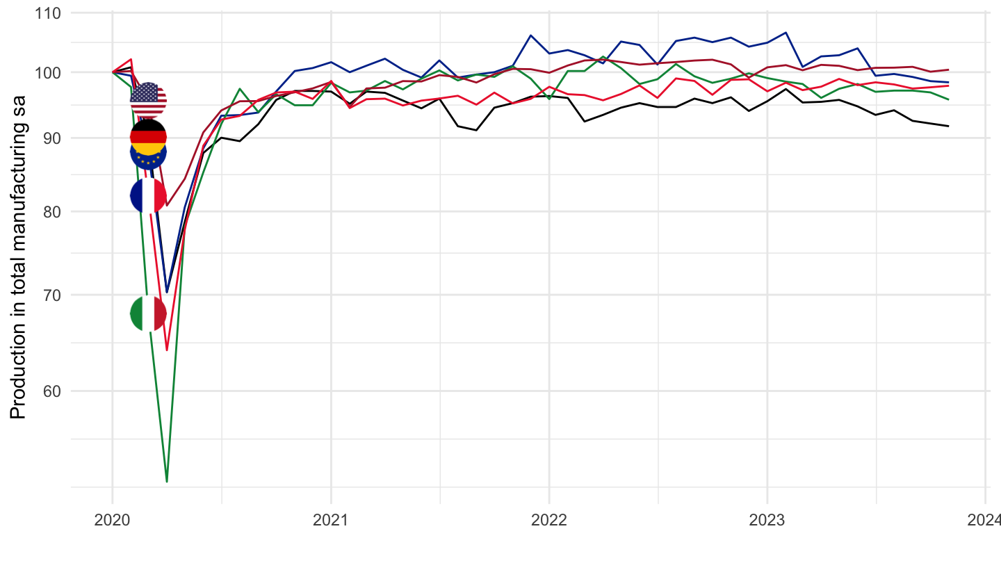
2019-
MEI_REAL %>%
  left_join(MEI_REAL_var$LOCATION, by = "LOCATION") %>%
  filter(SUBJECT == "PRMNTO01",
         FREQUENCY == "M",
         LOCATION %in% c("FRA", "DEU", "ITA", "USA", "EA20")) %>%
  month_to_date %>%
  filter(date >= as.Date("2019-01-01")) %>%
  group_by(Location) %>%
  mutate(obsValue = 100*obsValue/obsValue[date == as.Date("2019-01-01")]) %>%
  mutate(Location = ifelse(LOCATION == "EA20", "Europe", Location)) %>%
  left_join(colors, by = c("Location" = "country")) %>%
  mutate(color = ifelse(LOCATION == "USA", color2, color)) %>%
  ggplot(.) + geom_line(aes(x = date, y = obsValue, color = color)) +
  scale_color_identity() + add_5flags +
  theme_minimal() + xlab("") + ylab("Production in total manufacturing sa") +
  scale_x_date(breaks = seq(1910, 2100, 1) %>% paste0("-01-01") %>% as.Date,
               labels = date_format("%Y")) +
  scale_y_log10(breaks = seq(-10, 300, 10),
                     labels = dollar_format(accuracy = 1, prefix = "")) +
  theme(legend.position = c(0.2, 0.80),
        legend.title = element_blank())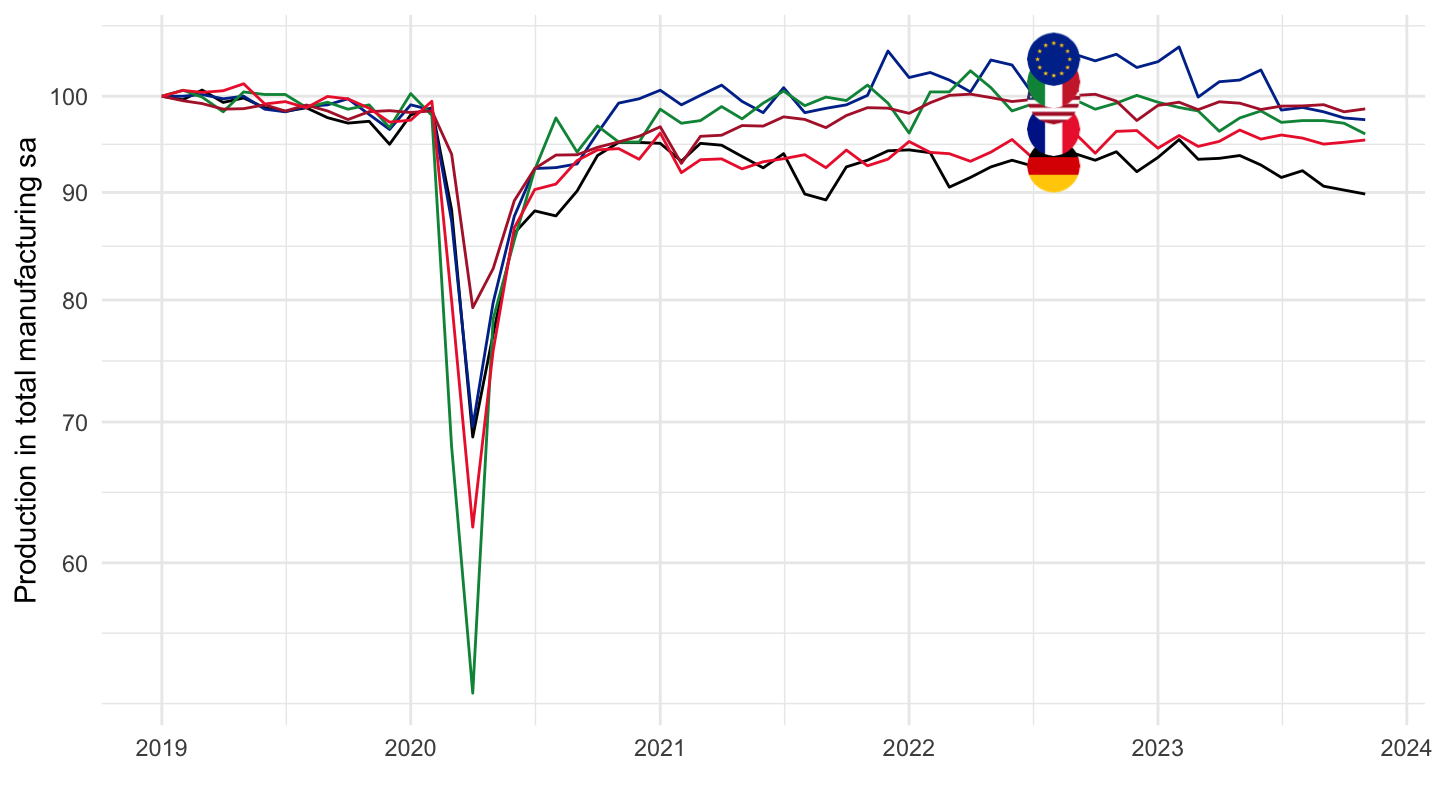
2019Q4-
MEI_REAL %>%
  left_join(MEI_REAL_var$LOCATION, by = "LOCATION") %>%
  filter(SUBJECT == "PRMNTO01",
         FREQUENCY == "M",
         LOCATION %in% c("FRA", "DEU", "ITA", "USA", "EA20")) %>%
  month_to_date %>%
  filter(date >= as.Date("2019-10-01")) %>%
  group_by(Location) %>%
  mutate(obsValue = 100*obsValue/obsValue[date == as.Date("2019-10-01")]) %>%
  mutate(Location = ifelse(LOCATION == "EA20", "Europe", Location)) %>%
  left_join(colors, by = c("Location" = "country")) %>%
  mutate(color = ifelse(LOCATION == "USA", color2, color)) %>%
  ggplot(.) + geom_line(aes(x = date, y = obsValue, color = color)) +
  scale_color_identity() + add_5flags +
  theme_minimal() + xlab("") + ylab("Production in total manufacturing sa") +
  scale_x_date(breaks = seq(1910, 2100, 1) %>% paste0("-01-01") %>% as.Date,
               labels = date_format("%Y")) +
  scale_y_log10(breaks = seq(-10, 300, 10),
                     labels = dollar_format(accuracy = 1, prefix = "")) +
  theme(legend.position = c(0.2, 0.80),
        legend.title = element_blank())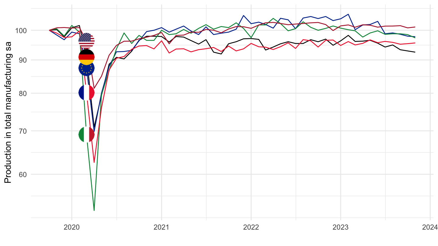
France, Germany, Italy, United States
Quarterly
All
MEI_REAL %>%
  left_join(MEI_REAL_var$LOCATION, by = "LOCATION") %>%
  filter(SUBJECT == "PRMNTO01",
         FREQUENCY == "Q",
         LOCATION %in% c("FRA", "DEU", "ITA", "USA")) %>%
  quarter_to_date %>%
  left_join(colors, by = c("Location" = "country")) %>%
  ggplot(.) + geom_line(aes(x = date, y = obsValue, color = color)) +
  scale_color_identity() + add_4flags +
  theme_minimal() + xlab("") + ylab("Passenger car registrations") +
  scale_x_date(breaks = seq(1910, 2100, 10) %>% paste0("-01-01") %>% as.Date,
               labels = date_format("%Y")) +
  scale_y_log10(breaks = seq(-10, 300, 10),
                     labels = dollar_format(accuracy = 1, prefix = "")) +
  theme(legend.position = c(0.2, 0.80),
        legend.title = element_blank())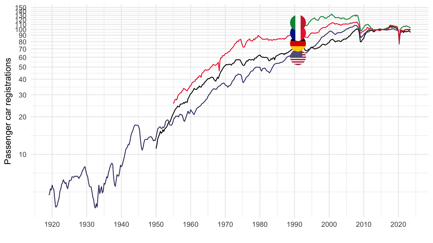
1955-
MEI_REAL %>%
  left_join(MEI_REAL_var$LOCATION, by = "LOCATION") %>%
  filter(SUBJECT == "PRMNTO01",
         FREQUENCY == "Q",
         LOCATION %in% c("FRA", "DEU", "ITA", "USA")) %>%
  quarter_to_date %>%
  filter(date >= as.Date("1955-01-01")) %>%
  left_join(colors, by = c("Location" = "country")) %>%
  ggplot(.) + geom_line(aes(x = date, y = obsValue, color = color)) +
  scale_color_identity() + add_4flags +
  theme_minimal() + xlab("") + ylab("Passenger car registrations") +
  scale_x_date(breaks = seq(1910, 2100, 10) %>% paste0("-01-01") %>% as.Date,
               labels = date_format("%Y")) +
  scale_y_log10(breaks = seq(-10, 300, 10),
                     labels = dollar_format(accuracy = 1, prefix = "")) +
  theme(legend.position = c(0.2, 0.80),
        legend.title = element_blank())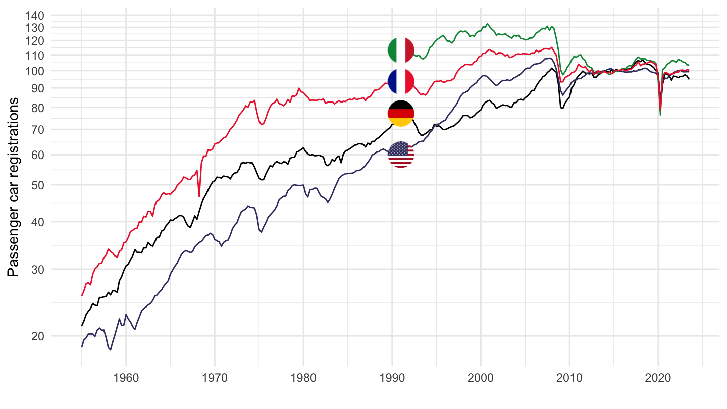
1975-
MEI_REAL %>%
  left_join(MEI_REAL_var$LOCATION, by = "LOCATION") %>%
  filter(SUBJECT == "PRMNTO01",
         FREQUENCY == "Q",
         LOCATION %in% c("FRA", "DEU", "ITA", "USA")) %>%
  quarter_to_date %>%
  filter(date >= as.Date("1975-01-01")) %>%
  left_join(colors, by = c("Location" = "country")) %>%
  ggplot(.) + geom_line(aes(x = date, y = obsValue, color = color)) +
  scale_color_identity() + add_4flags +
  theme_minimal() + xlab("") + ylab("Passenger car registrations") +
  scale_x_date(breaks = seq(1910, 2100, 10) %>% paste0("-01-01") %>% as.Date,
               labels = date_format("%Y")) +
  scale_y_log10(breaks = seq(-10, 300, 10),
                     labels = dollar_format(accuracy = 1, prefix = "")) +
  theme(legend.position = c(0.2, 0.80),
        legend.title = element_blank())
1990-
MEI_REAL %>%
  left_join(MEI_REAL_var$LOCATION, by = "LOCATION") %>%
  filter(SUBJECT == "PRMNTO01",
         FREQUENCY == "Q",
         LOCATION %in% c("FRA", "DEU", "ITA", "USA")) %>%
  quarter_to_date %>%
  filter(date >= as.Date("1990-01-01")) %>%
  left_join(colors, by = c("Location" = "country")) %>%
  ggplot(.) + geom_line(aes(x = date, y = obsValue, color = color)) +
  scale_color_identity() + add_4flags +
  theme_minimal() + xlab("") + ylab("Passenger car registrations") +
  scale_x_date(breaks = seq(1910, 2100, 10) %>% paste0("-01-01") %>% as.Date,
               labels = date_format("%Y")) +
  scale_y_log10(breaks = seq(-10, 300, 10),
                     labels = dollar_format(accuracy = 1, prefix = "")) +
  theme(legend.position = c(0.2, 0.80),
        legend.title = element_blank())
Monthly
All
MEI_REAL %>%
  left_join(MEI_REAL_var$LOCATION, by = "LOCATION") %>%
  filter(SUBJECT == "PRMNTO01",
         FREQUENCY == "M",
         LOCATION %in% c("FRA", "DEU", "ITA", "USA")) %>%
  month_to_date %>%
  left_join(colors, by = c("Location" = "country")) %>%
  ggplot(.) + geom_line(aes(x = date, y = obsValue, color = color)) +
  scale_color_identity() + add_4flags +
  theme_minimal() + xlab("") + ylab("Passenger car registrations") +
  scale_x_date(breaks = seq(1910, 2100, 5) %>% paste0("-01-01") %>% as.Date,
               labels = date_format("%Y")) +
  scale_y_log10(breaks = seq(-10, 300, 10),
                     labels = dollar_format(accuracy = 1, prefix = "")) +
  theme(legend.position = c(0.2, 0.80),
        legend.title = element_blank())
1990-
MEI_REAL %>%
  left_join(MEI_REAL_var$LOCATION, by = "LOCATION") %>%
  filter(SUBJECT == "PRMNTO01",
         FREQUENCY == "M",
         LOCATION %in% c("FRA", "DEU", "ITA", "USA")) %>%
  month_to_date %>%
  filter(date >= as.Date("1990-01-01")) %>%
  group_by(Location) %>%
  mutate(obsValue = 100*obsValue/obsValue[date == as.Date("1990-01-01")]) %>%
  left_join(colors, by = c("Location" = "country")) %>%
  mutate(color = ifelse(LOCATION == "USA", color2, color)) %>%
  ggplot(.) + geom_line(aes(x = date, y = obsValue, color = color)) +
  scale_color_identity() + add_4flags +
  theme_minimal() + xlab("") + ylab("Production in total manufacturing sa") +
  scale_x_date(breaks = seq(1910, 2100, 2) %>% paste0("-01-01") %>% as.Date,
               labels = date_format("%Y")) +
  scale_y_log10(breaks = seq(-10, 300, 10),
                     labels = dollar_format(accuracy = 1, prefix = "")) +
  theme(legend.position = c(0.2, 0.80),
        legend.title = element_blank())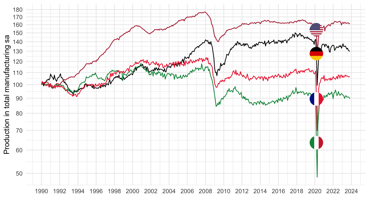
1995-
English
MEI_REAL %>%
  left_join(MEI_REAL_var$LOCATION, by = "LOCATION") %>%
  filter(SUBJECT == "PRMNTO01",
         FREQUENCY == "M",
         LOCATION %in% c("FRA", "DEU", "ITA", "USA")) %>%
  month_to_date %>%
  filter(date >= as.Date("1995-01-01")) %>%
  group_by(Location) %>%
  mutate(obsValue = 100*obsValue/obsValue[date == as.Date("1995-01-01")]) %>%
  left_join(colors, by = c("Location" = "country")) %>%
  mutate(color = ifelse(LOCATION == "USA", color2, color)) %>%
  ggplot(.) + geom_line(aes(x = date, y = obsValue, color = color)) +
  scale_color_identity() + add_4flags +
  theme_minimal() + xlab("") + ylab("Production in total manufacturing sa") +
  scale_x_date(breaks = seq(1910, 2100, 5) %>% paste0("-01-01") %>% as.Date,
               labels = date_format("%Y")) +
  scale_y_log10(breaks = seq(-10, 300, 10),
                     labels = dollar_format(accuracy = 1, prefix = "")) +
  theme(legend.position = c(0.2, 0.80),
        legend.title = element_blank())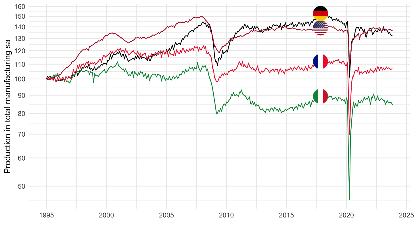
French
MEI_REAL %>%
  left_join(MEI_REAL_var$LOCATION, by = "LOCATION") %>%
  filter(SUBJECT == "PRMNTO01",
         FREQUENCY == "M",
         LOCATION %in% c("FRA", "DEU", "ITA", "USA")) %>%
  month_to_date %>%
  filter(date >= as.Date("1995-01-01")) %>%
  group_by(Location) %>%
  mutate(obsValue = 100*obsValue/obsValue[date == as.Date("1995-01-01")]) %>%
  left_join(colors, by = c("Location" = "country")) %>%
  mutate(color = ifelse(LOCATION == "USA", color2, color)) %>%
  ggplot(.) + geom_line(aes(x = date, y = obsValue, color = color)) +
  scale_color_identity() + add_4flags +
  theme_minimal() + xlab("") + ylab("Production dans l'industrie manufacturière (1995 = 100)") +
  scale_x_date(breaks = seq(1910, 2100, 5) %>% paste0("-01-01") %>% as.Date,
               labels = date_format("%Y")) +
  scale_y_log10(breaks = seq(-10, 300, 10),
                     labels = dollar_format(accuracy = 1, prefix = "")) +
  theme(legend.position = c(0.2, 0.80),
        legend.title = element_blank())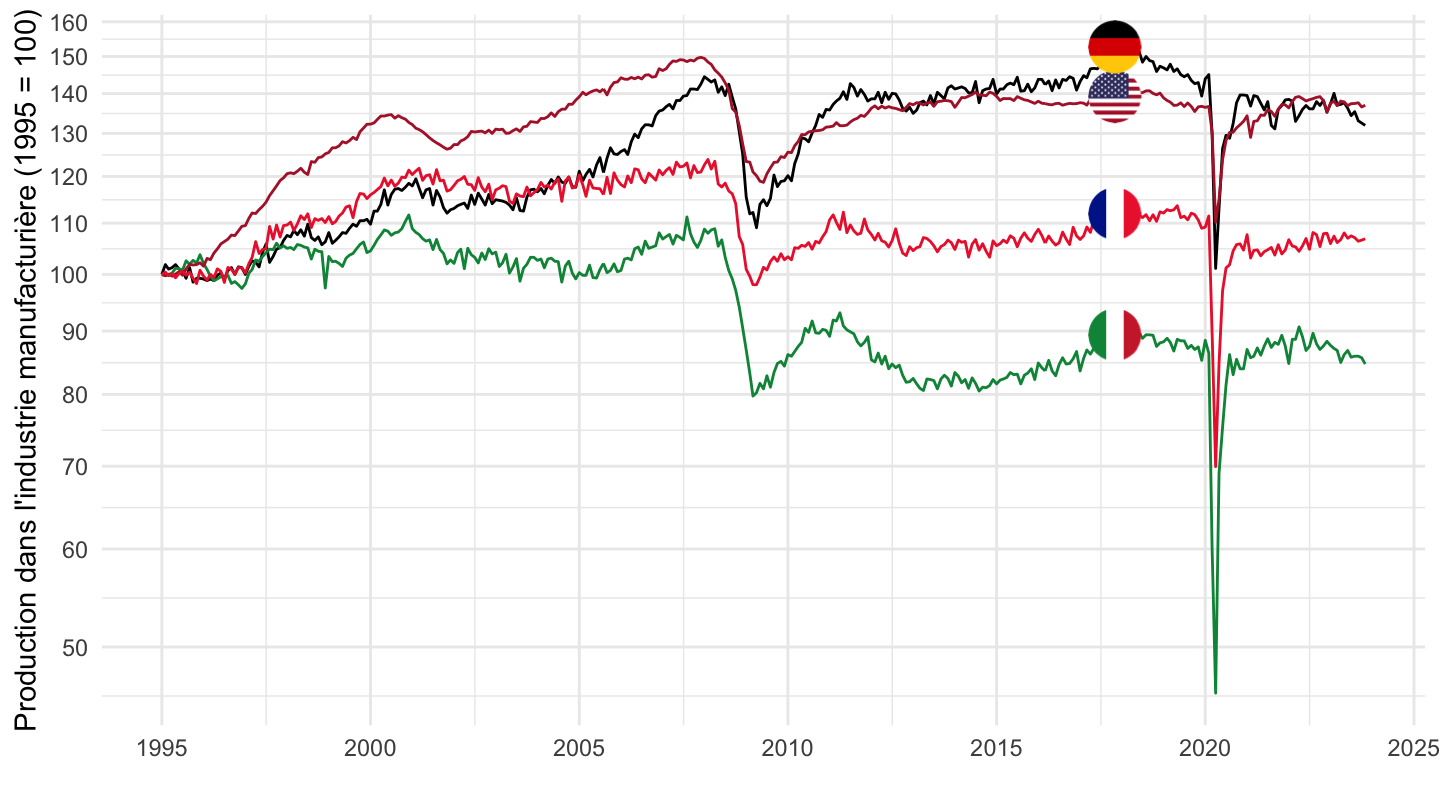
1998-
MEI_REAL %>%
  left_join(MEI_REAL_var$LOCATION, by = "LOCATION") %>%
  filter(SUBJECT == "PRMNTO01",
         FREQUENCY == "M",
         LOCATION %in% c("FRA", "DEU", "ITA", "USA")) %>%
  month_to_date %>%
  filter(date >= as.Date("1998-01-01")) %>%
  group_by(Location) %>%
  mutate(obsValue = 100*obsValue/obsValue[date == as.Date("1998-01-01")]) %>%
  left_join(colors, by = c("Location" = "country")) %>%
  mutate(color = ifelse(LOCATION == "USA", color2, color)) %>%
  ggplot(.) + geom_line(aes(x = date, y = obsValue, color = color)) +
  scale_color_identity() + add_4flags +
  theme_minimal() + xlab("") + ylab("Production in total manufacturing sa") +
  scale_x_date(breaks = seq(1910, 2100, 2) %>% paste0("-01-01") %>% as.Date,
               labels = date_format("%Y")) +
  scale_y_log10(breaks = seq(-10, 300, 10),
                     labels = dollar_format(accuracy = 1, prefix = "")) +
  theme(legend.position = c(0.2, 0.80),
        legend.title = element_blank())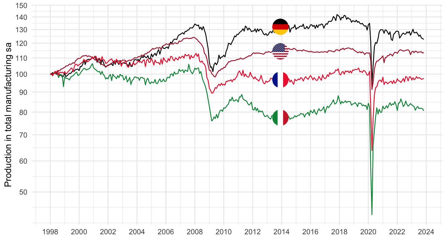
2017Q2-
MEI_REAL %>%
  left_join(MEI_REAL_var$LOCATION, by = "LOCATION") %>%
  filter(SUBJECT == "PRMNTO01",
         FREQUENCY == "M",
         LOCATION %in% c("FRA", "DEU", "ITA", "USA")) %>%
  month_to_date %>%
  filter(date >= as.Date("2017-04-01")) %>%
  group_by(Location) %>%
  mutate(obsValue = 100*obsValue/obsValue[date == as.Date("2017-04-01")]) %>%
  left_join(colors, by = c("Location" = "country")) %>%
  mutate(color = ifelse(LOCATION == "USA", color2, color)) %>%
  ggplot(.) + geom_line(aes(x = date, y = obsValue, color = color)) +
  scale_color_identity() + add_4flags +
  theme_minimal() + xlab("") + ylab("Production in total manufacturing sa") +
  scale_x_date(breaks = "6 months",
               labels = date_format("%b %y")) +
  scale_y_log10(breaks = seq(-10, 300, 10),
                     labels = dollar_format(accuracy = 1, prefix = ""))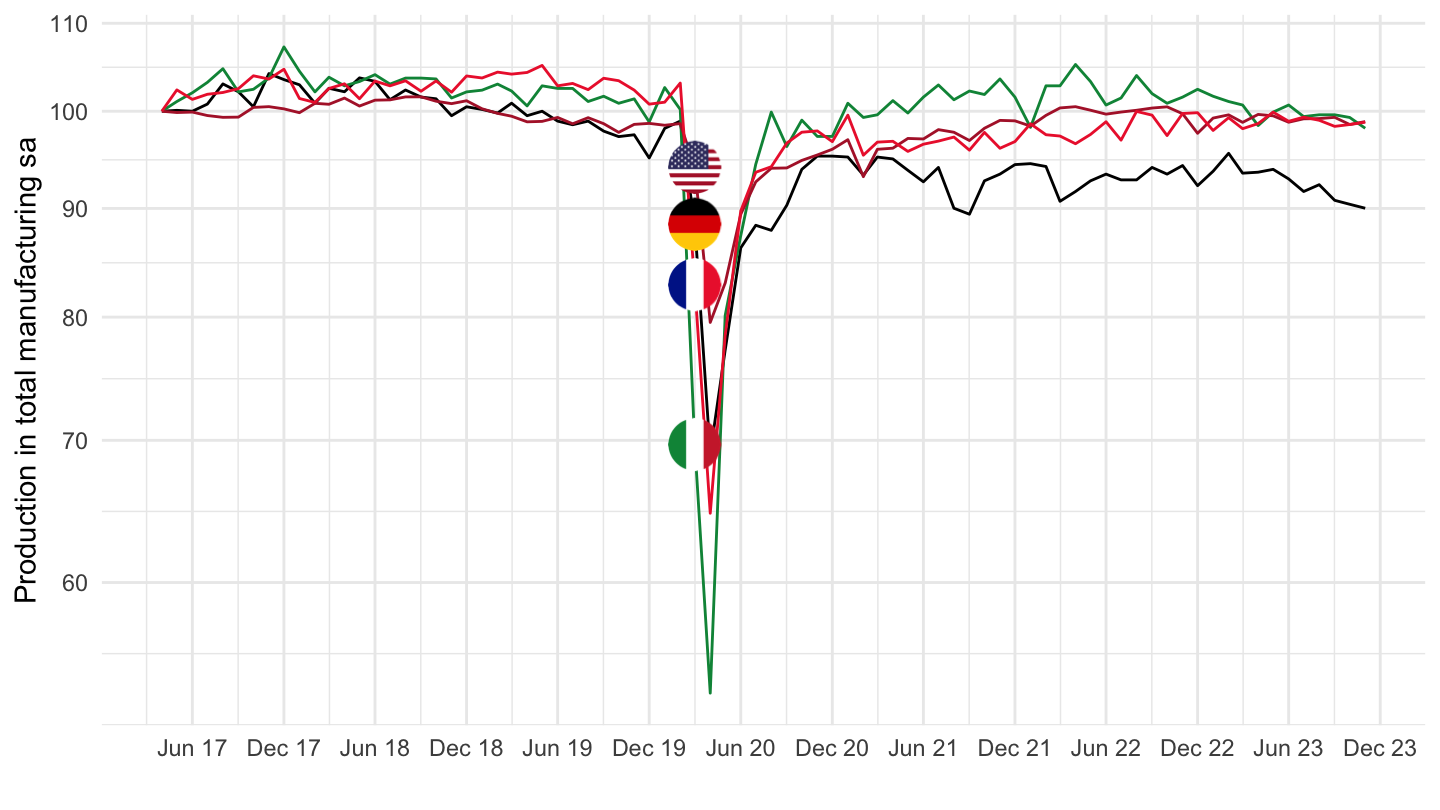
2020-02-
MEI_REAL %>%
left_join(MEI_REAL_var$LOCATION, by = "LOCATION") %>%
filter(SUBJECT == "PRMNTO01",
FREQUENCY == "M",
LOCATION %in% c("FRA", "DEU", "ITA", "USA")) %>%
month_to_date %>%
filter(date >= as.Date("2020-02-01")) %>%
group_by(Location) %>%
mutate(obsValue = 100*obsValue/obsValue[date == as.Date("2020-02-01")]) %>%
left_join(colors, by = c("Location" = "country")) %>%
mutate(color = ifelse(LOCATION == "USA", color2, color)) %>%
ggplot(.) + geom_line(aes(x = date, y = obsValue, color = color)) +
scale_color_identity() + add_4flags +
theme_minimal() + xlab("") + ylab("Production in total manufacturing sa") +
scale_x_date(breaks = "3 months",
labels = date_format("%b %y")) +
scale_y_log10(breaks = seq(-10, 300, 10),
labels = dollar_format(accuracy = 1, prefix = ""))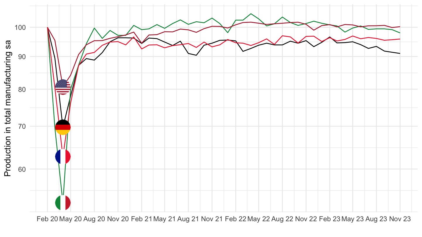 ## France, Italy, Belgium, Germany
Monthly
All
MEI_REAL %>%
  left_join(MEI_REAL_var$LOCATION, by = "LOCATION") %>%
  filter(SUBJECT == "PRMNTO01",
         FREQUENCY == "M",
         LOCATION %in% c("FRA", "DEU", "ITA", "USA", "BEL")) %>%
  month_to_date %>%
  left_join(colors, by = c("Location" = "country")) %>%
  ggplot(.) + geom_line(aes(x = date, y = obsValue, color = color)) +
  scale_color_identity() + add_5flags +
  theme_minimal() + xlab("") + ylab("Passenger car registrations") +
  scale_x_date(breaks = seq(1910, 2100, 10) %>% paste0("-01-01") %>% as.Date,
               labels = date_format("%Y")) +
  scale_y_log10(breaks = seq(-10, 300, 10),
                     labels = dollar_format(accuracy = 1, prefix = "")) +
  theme(legend.position = c(0.2, 0.80),
        legend.title = element_blank())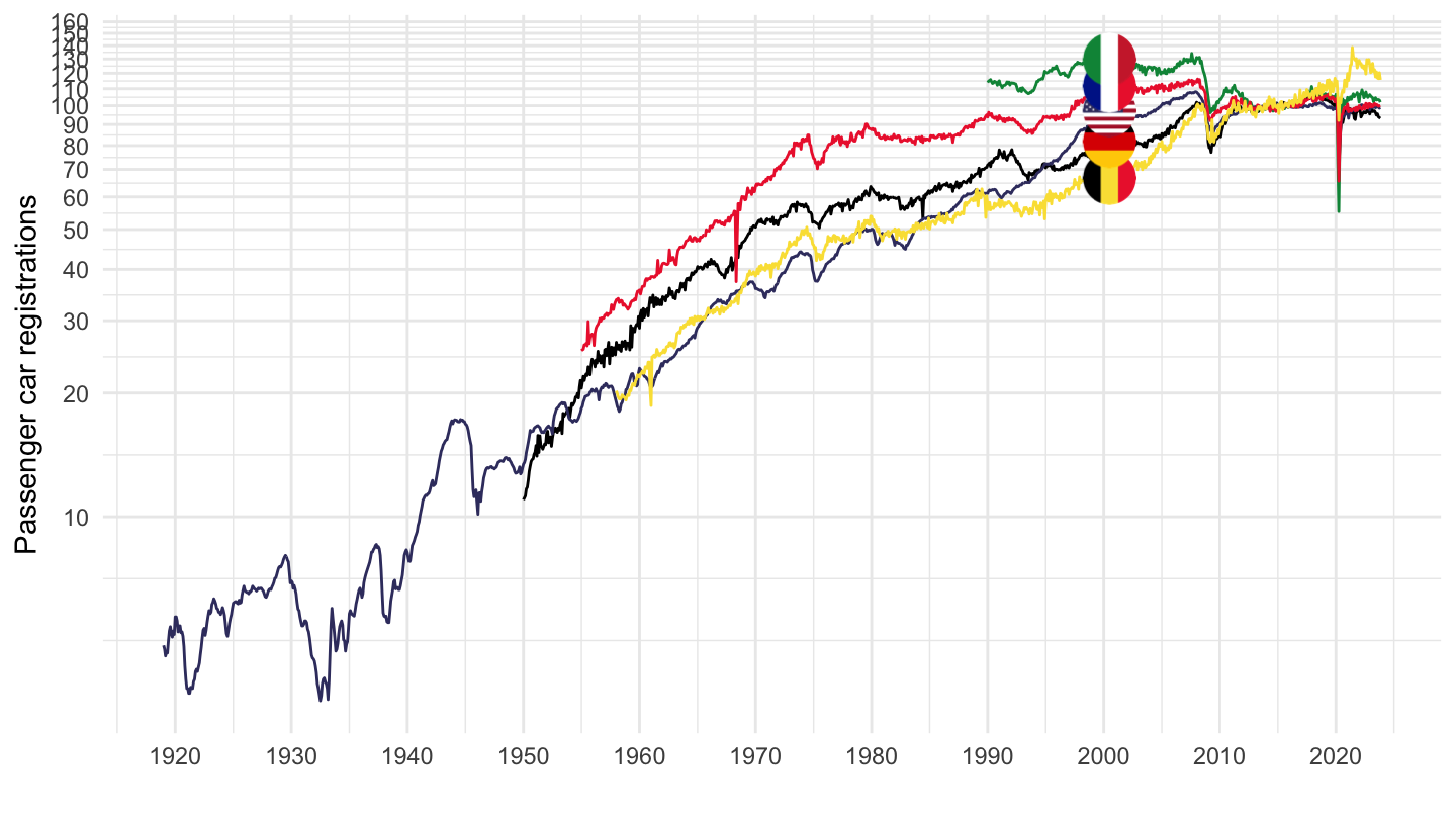
1990-
MEI_REAL %>%
  left_join(MEI_REAL_var$LOCATION, by = "LOCATION") %>%
  filter(SUBJECT == "PRMNTO01",
         FREQUENCY == "M",
         LOCATION %in% c("FRA", "DEU", "ITA", "USA", "BEL")) %>%
  month_to_date %>%
  filter(date >= as.Date("1990-01-01")) %>%
  group_by(Location) %>%
  mutate(obsValue = 100*obsValue/obsValue[date == as.Date("1990-01-01")]) %>%
  left_join(colors, by = c("Location" = "country")) %>%
  mutate(color = ifelse(LOCATION == "USA", color2, color)) %>%
  ggplot(.) + geom_line(aes(x = date, y = obsValue, color = color)) +
  scale_color_identity() + add_5flags +
  theme_minimal() + xlab("") + ylab("Production in total manufacturing sa") +
  scale_x_date(breaks = seq(1910, 2100, 5) %>% paste0("-01-01") %>% as.Date,
               labels = date_format("%Y")) +
  scale_y_log10(breaks = seq(-10, 300, 10),
                     labels = dollar_format(accuracy = 1, prefix = "")) +
  theme(legend.position = c(0.2, 0.80),
        legend.title = element_blank())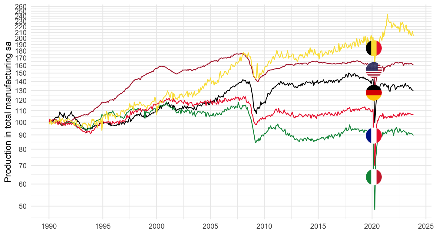
2002-
MEI_REAL %>%
  left_join(MEI_REAL_var$LOCATION, by = "LOCATION") %>%
  filter(SUBJECT == "PRMNTO01",
         FREQUENCY == "M",
         LOCATION %in% c("FRA", "DEU", "ITA", "USA", "BEL")) %>%
  month_to_date %>%
  filter(date >= as.Date("2002-01-01")) %>%
  group_by(Location) %>%
  mutate(obsValue = 100*obsValue/obsValue[date == as.Date("2002-01-01")]) %>%
  left_join(colors, by = c("Location" = "country")) %>%
  #mutate(color = ifelse(LOCATION == "FRA", color2, color)) %>%
  ggplot(.) + geom_line(aes(x = date, y = obsValue, color = color)) +
  scale_color_identity() + add_5flags +
  theme_minimal() + xlab("") + ylab("Production in total manufacturing sa") +
  scale_x_date(breaks = seq(1910, 2024, 2) %>% paste0("-01-01") %>% as.Date,
               labels = date_format("%Y")) +
  scale_y_log10(breaks = seq(-10, 300, 10),
                     labels = dollar_format(accuracy = 1, prefix = "")) +
  theme(legend.position = c(0.2, 0.80),
        legend.title = element_blank())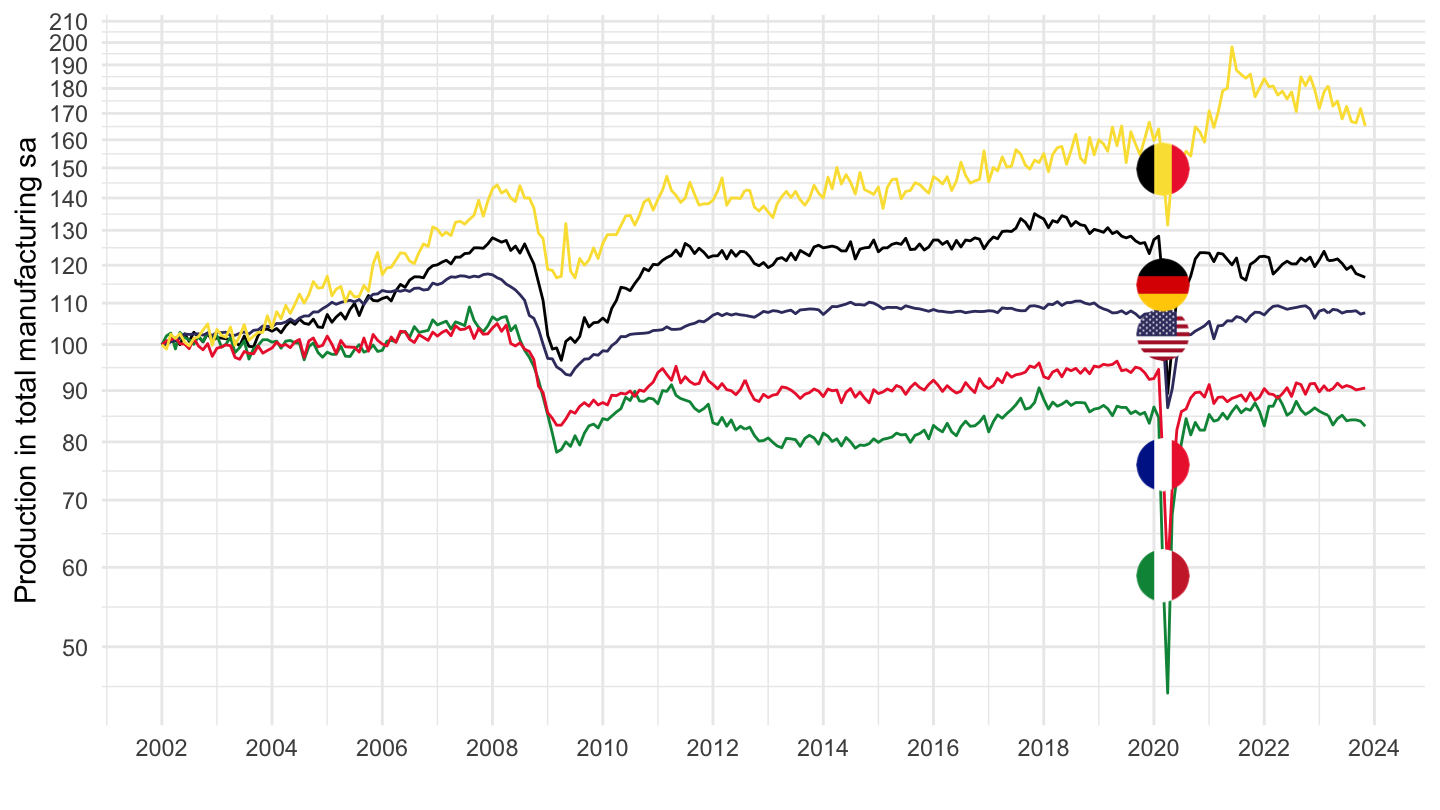
Production in total industry, Index - PRINTO01
France, Germany, Italy, United States, Spain, Switzerland
Monthly
All
MEI_REAL %>%
  left_join(MEI_REAL_var$LOCATION, by = "LOCATION") %>%
  filter(SUBJECT == "PRINTO01",
         FREQUENCY == "M",
         LOCATION %in% c("FRA", "DEU", "ITA", "USA", "ESP")) %>%
  month_to_date %>%
  #filter(date >= as.Date("1990-01-01")) %>%
  group_by(Location) %>%
  mutate(obsValue = 100*obsValue/obsValue[date == as.Date("1990-01-01")]) %>%
  left_join(colors, by = c("Location" = "country")) %>%
  mutate(color = ifelse(LOCATION == "USA", color2, color)) %>%
  ggplot(.) + geom_line(aes(x = date, y = obsValue, color = color)) +
  scale_color_identity() + add_5flags +
  theme_minimal() + xlab("") + ylab("Production in total industry sa") +
  scale_x_date(breaks = seq(1910, 2100, 10) %>% paste0("-01-01") %>% as.Date,
               labels = date_format("%Y")) +
  scale_y_log10(breaks = seq(-10, 300, 10),
                     labels = dollar_format(accuracy = 1, prefix = ""))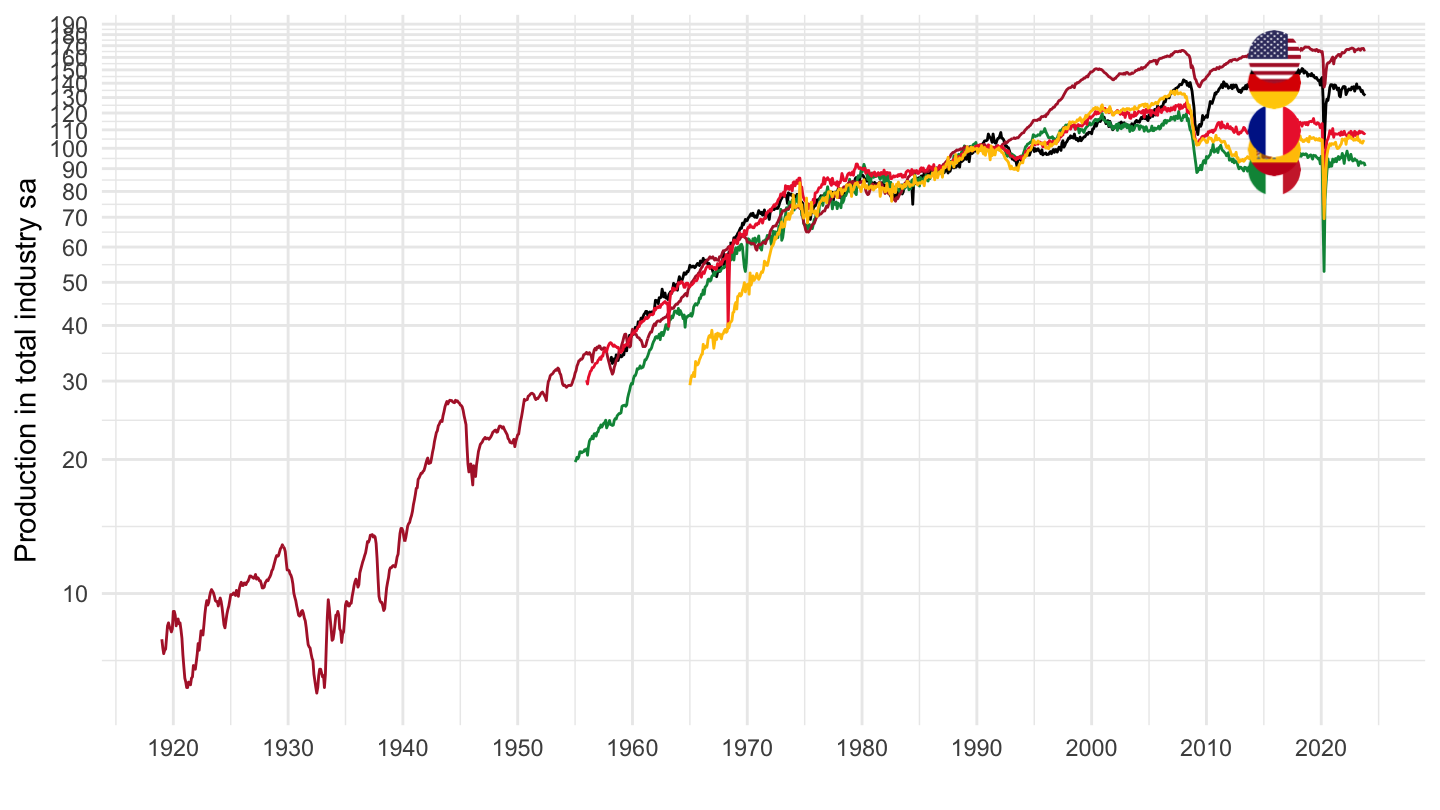
1990-
MEI_REAL %>%
  left_join(MEI_REAL_var$LOCATION, by = "LOCATION") %>%
  filter(SUBJECT == "PRINTO01",
         FREQUENCY == "M",
         LOCATION %in% c("FRA", "DEU", "ITA", "USA", "ESP")) %>%
  month_to_date %>%
  filter(date >= as.Date("1990-01-01")) %>%
  group_by(Location) %>%
  mutate(obsValue = 100*obsValue/obsValue[date == as.Date("1990-01-01")]) %>%
  left_join(colors, by = c("Location" = "country")) %>%
  mutate(color = ifelse(LOCATION == "USA", color2, color)) %>%
  ggplot(.) + geom_line(aes(x = date, y = obsValue, color = color)) +
  scale_color_identity() + add_5flags +
  theme_minimal() + xlab("") + ylab("Production in total industry sa") +
  scale_x_date(breaks = seq(1910, 2100, 2) %>% paste0("-01-01") %>% as.Date,
               labels = date_format("%Y")) +
  scale_y_log10(breaks = seq(-10, 300, 10),
                     labels = dollar_format(accuracy = 1, prefix = ""))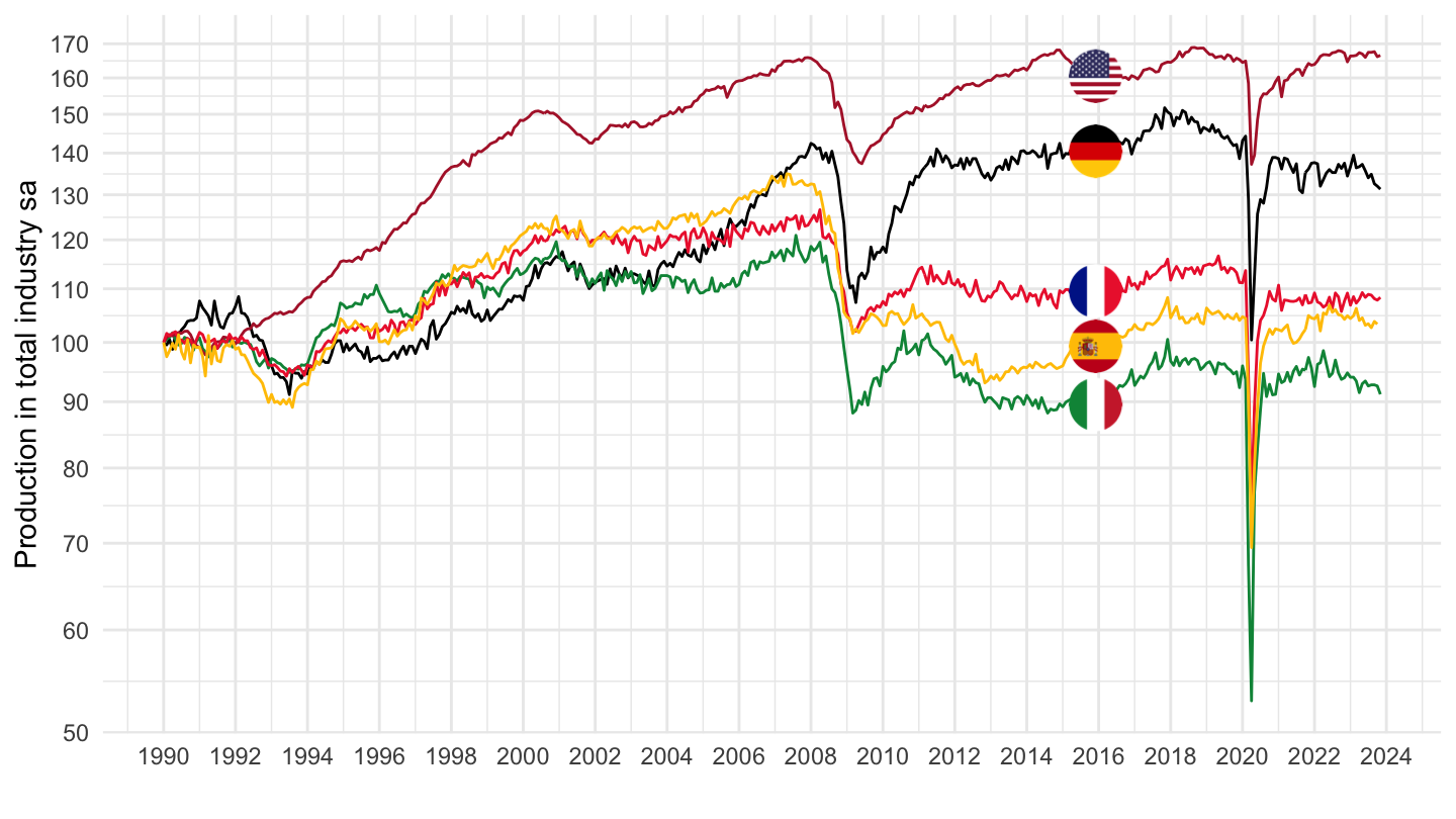
France, Germany, Italy, United States
Monthly
1990-
MEI_REAL %>%
  left_join(MEI_REAL_var$LOCATION, by = "LOCATION") %>%
  filter(SUBJECT == "PRINTO01",
         FREQUENCY == "M",
         LOCATION %in% c("FRA", "DEU", "ITA", "USA")) %>%
  month_to_date %>%
  filter(date >= as.Date("1990-01-01")) %>%
  group_by(Location) %>%
  mutate(obsValue = 100*obsValue/obsValue[date == as.Date("1990-01-01")]) %>%
  left_join(colors, by = c("Location" = "country")) %>%
  mutate(color = ifelse(LOCATION == "USA", color2, color)) %>%
  ggplot(.) + geom_line(aes(x = date, y = obsValue, color = color)) +
  scale_color_identity() + add_4flags +
  theme_minimal() + xlab("") + ylab("Production in total industry sa") +
  scale_x_date(breaks = seq(1910, 2100, 5) %>% paste0("-01-01") %>% as.Date,
               labels = date_format("%Y")) +
  scale_y_log10(breaks = seq(-10, 300, 10),
                     labels = dollar_format(accuracy = 1, prefix = ""))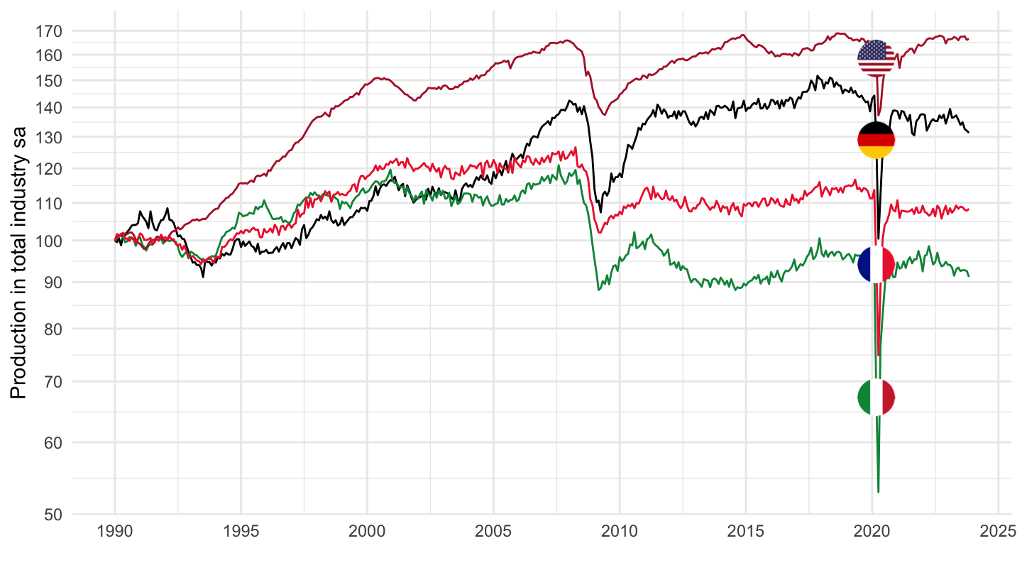
1995-
MEI_REAL %>%
  left_join(MEI_REAL_var$LOCATION, by = "LOCATION") %>%
  filter(SUBJECT == "PRINTO01",
         FREQUENCY == "M",
         LOCATION %in% c("FRA", "DEU", "ITA", "USA")) %>%
  month_to_date %>%
  filter(date >= as.Date("1995-01-01")) %>%
  group_by(Location) %>%
  mutate(obsValue = 100*obsValue/obsValue[date == as.Date("1995-01-01")]) %>%
  left_join(colors, by = c("Location" = "country")) %>%
  mutate(color = ifelse(LOCATION == "USA", color2, color)) %>%
  ggplot(.) + geom_line(aes(x = date, y = obsValue, color = color)) +
  scale_color_identity() + add_4flags +
  theme_minimal() + xlab("") + ylab("Production in total industry, index") +
  scale_x_date(breaks = seq(1910, 2100, 2) %>% paste0("-01-01") %>% as.Date,
               labels = date_format("%Y")) +
  scale_y_log10(breaks = seq(-10, 300, 10),
                     labels = dollar_format(accuracy = 1, prefix = ""))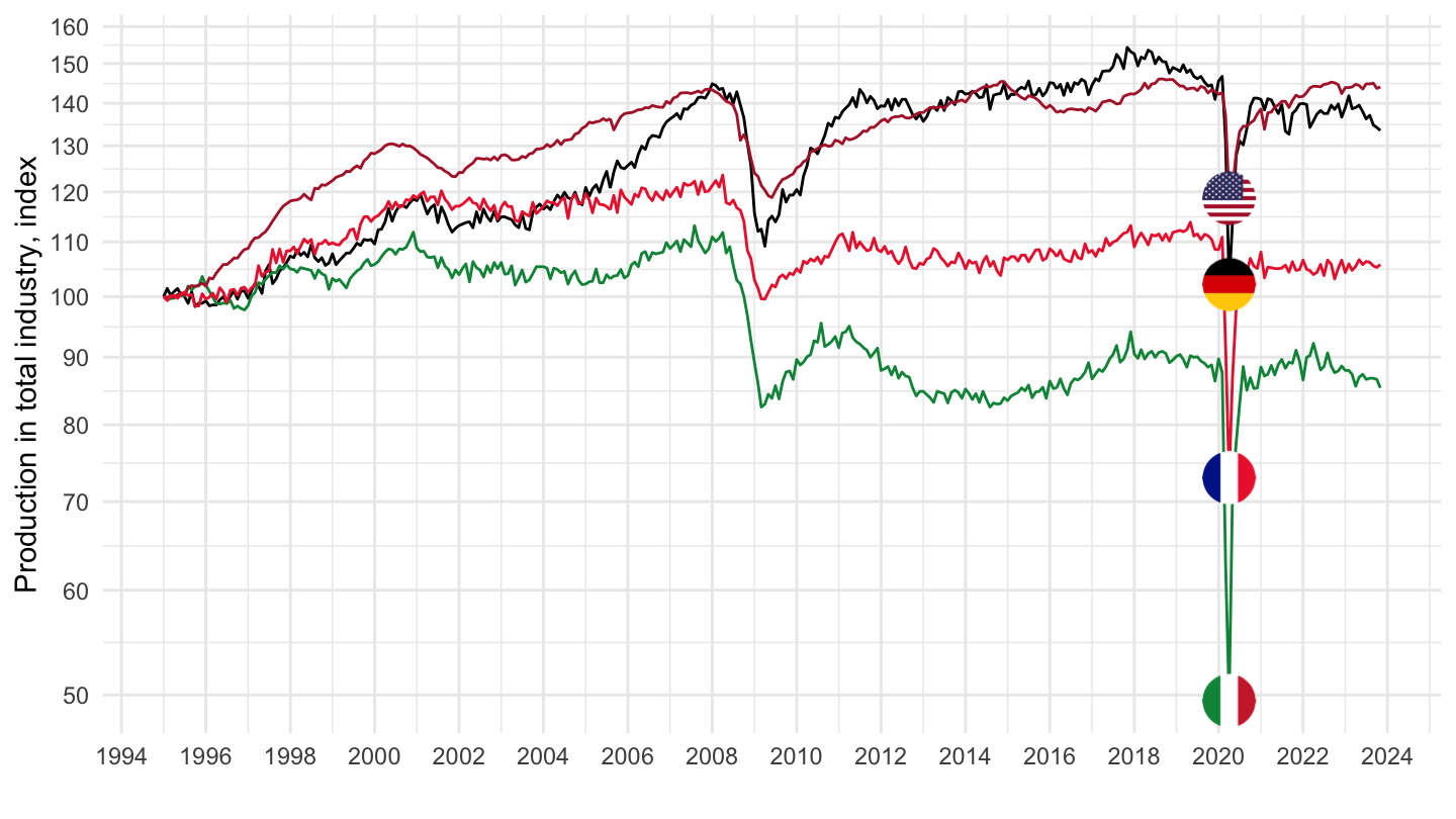
1998-
MEI_REAL %>%
  left_join(MEI_REAL_var$LOCATION, by = "LOCATION") %>%
  filter(SUBJECT == "PRINTO01",
         FREQUENCY == "M",
         LOCATION %in% c("FRA", "DEU", "ITA", "USA")) %>%
  month_to_date %>%
  filter(date >= as.Date("1998-01-01")) %>%
  group_by(Location) %>%
  mutate(obsValue = 100*obsValue/obsValue[date == as.Date("1998-01-01")]) %>%
  left_join(colors, by = c("Location" = "country")) %>%
  mutate(color = ifelse(LOCATION == "USA", color2, color)) %>%
  ggplot(.) + geom_line(aes(x = date, y = obsValue, color = color)) +
  scale_color_identity() + add_4flags +
  theme_minimal() + xlab("") + ylab("Production in total industry, index") +
  scale_x_date(breaks = seq(1910, 2100, 2) %>% paste0("-01-01") %>% as.Date,
               labels = date_format("%Y")) +
  scale_y_log10(breaks = seq(-10, 300, 10),
                     labels = dollar_format(accuracy = 1, prefix = ""))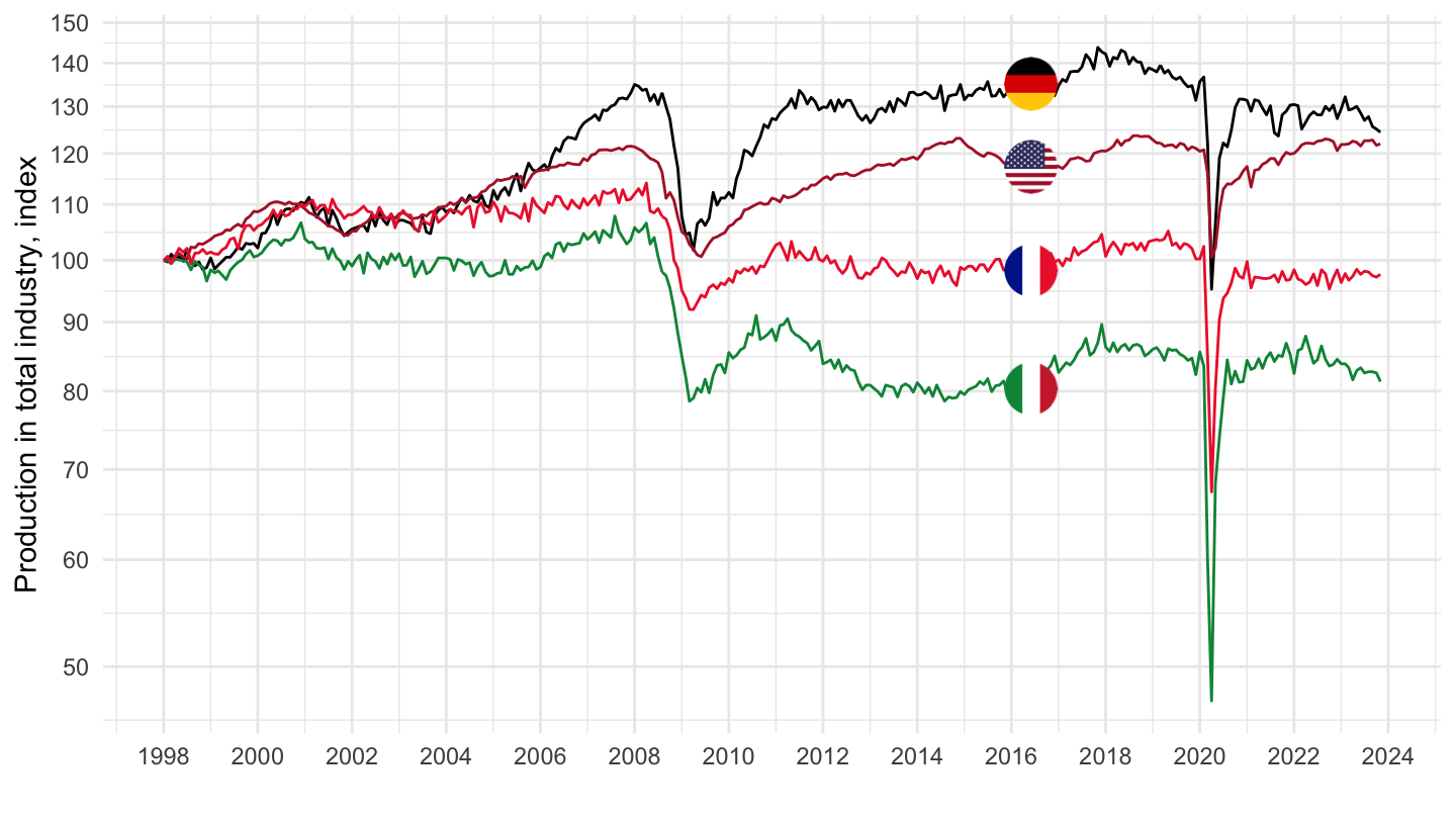
1999-
MEI_REAL %>%
  left_join(MEI_REAL_var$LOCATION, by = "LOCATION") %>%
  filter(SUBJECT == "PRINTO01",
         FREQUENCY == "M",
         LOCATION %in% c("FRA", "DEU", "ITA", "USA")) %>%
  month_to_date %>%
  filter(date >= as.Date("1999-01-01")) %>%
  group_by(Location) %>%
  mutate(obsValue = 100*obsValue/obsValue[date == as.Date("1999-01-01")]) %>%
  left_join(colors, by = c("Location" = "country")) %>%
  mutate(color = ifelse(LOCATION == "USA", color2, color)) %>%
  ggplot(.) + geom_line(aes(x = date, y = obsValue, color = color)) +
  scale_color_identity() + add_4flags +
  theme_minimal() + xlab("") + ylab("Production in total industry, index") +
  scale_x_date(breaks = seq(1910, 2100, 2) %>% paste0("-01-01") %>% as.Date,
               labels = date_format("%Y")) +
  scale_y_log10(breaks = seq(-10, 300, 10),
                     labels = dollar_format(accuracy = 1, prefix = ""))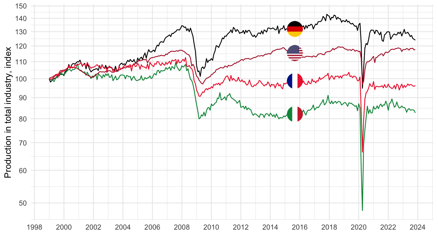
2017Q2-
MEI_REAL %>%
  left_join(MEI_REAL_var$LOCATION, by = "LOCATION") %>%
  filter(SUBJECT == "PRINTO01",
         FREQUENCY == "M",
         LOCATION %in% c("FRA", "DEU", "ITA", "USA")) %>%
  month_to_date %>%
  filter(date >= as.Date("2017-04-01")) %>%
  group_by(Location) %>%
  mutate(obsValue = 100*obsValue/obsValue[date == as.Date("2017-04-01")]) %>%
  left_join(colors, by = c("Location" = "country")) %>%
  mutate(color = ifelse(LOCATION == "USA", color2, color)) %>%
  ggplot(.) + geom_line(aes(x = date, y = obsValue, color = color)) +
  scale_color_identity() + add_4flags +
  theme_minimal() + xlab("") + ylab("Production in total industry, index") +
  scale_x_date(breaks = "6 months",
               labels = date_format("%b %y")) +
  scale_y_log10(breaks = seq(-10, 300, 10),
                     labels = dollar_format(accuracy = 1, prefix = ""))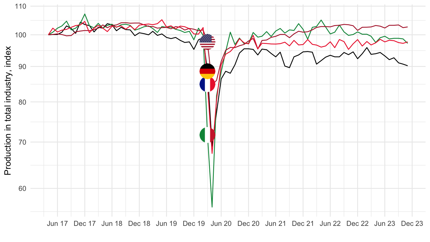
2020-02
MEI_REAL %>%
  left_join(MEI_REAL_var$LOCATION, by = "LOCATION") %>%
  filter(SUBJECT == "PRINTO01",
         FREQUENCY == "M",
         LOCATION %in% c("FRA", "DEU", "ITA", "USA")) %>%
  month_to_date %>%
  filter(date >= as.Date("2020-02-01")) %>%
  group_by(Location) %>%
  mutate(obsValue = 100*obsValue/obsValue[date == as.Date("2020-02-01")]) %>%
  left_join(colors, by = c("Location" = "country")) %>%
  mutate(color = ifelse(LOCATION == "USA", color2, color)) %>%
  ggplot(.) + geom_line(aes(x = date, y = obsValue, color = color)) +
  scale_color_identity() + add_4flags +
  theme_minimal() + xlab("") + ylab("Production in total industry, index") +
  scale_x_date(breaks = "3 months",
               labels = date_format("%b %y")) +
  scale_y_log10(breaks = seq(-10, 300, 10),
                     labels = dollar_format(accuracy = 1, prefix = ""))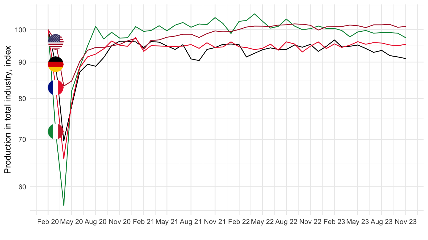
Quarterly
MEI_REAL %>%
  left_join(MEI_REAL_var$LOCATION, by = "LOCATION") %>%
  filter(SUBJECT == "PRINTO01",
         FREQUENCY == "Q",
         LOCATION %in% c("FRA", "DEU", "ITA", "USA")) %>%
  quarter_to_date %>%
  filter(date >= as.Date("1955-01-01")) %>%
  group_by(Location) %>%
  mutate(obsValue = 100*obsValue/obsValue[date == as.Date("1968-01-01")]) %>%
  left_join(colors, by = c("Location" = "country")) %>%
  ggplot(.) + geom_line(aes(x = date, y = obsValue, color = color)) +
  scale_color_identity() + add_4flags +
  theme_minimal() + xlab("") + ylab("Production in total industry") +
  scale_x_date(breaks = seq(1910, 2100, 5) %>% paste0("-01-01") %>% as.Date,
               labels = date_format("%Y")) +
  scale_y_log10(breaks = seq(0, 300, 20),
                     labels = dollar_format(accuracy = 1, prefix = "")) +
  theme(legend.position = c(0.2, 0.80),
        legend.title = element_blank())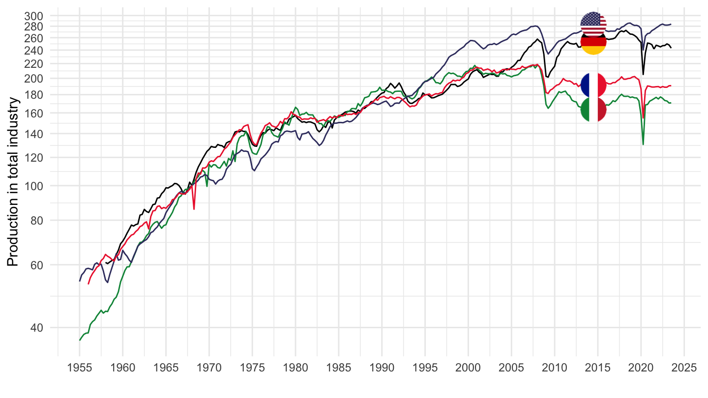
Germany, Portugal, Spain, UK
Quarterly
MEI_REAL %>%
  left_join(MEI_REAL_var$LOCATION, by = "LOCATION") %>%
  filter(SUBJECT == "PRINTO01",
         FREQUENCY == "Q",
         LOCATION %in% c("DEU", "PRT", "ESP", "GBR")) %>%
  quarter_to_date %>%
  filter(date >= as.Date("1955-01-01")) %>%
  group_by(Location) %>%
  mutate(obsValue = 100*obsValue/obsValue[date == as.Date("1968-01-01")]) %>%
  left_join(colors, by = c("Location" = "country")) %>%
  ggplot(.) + geom_line(aes(x = date, y = obsValue, color = color)) +
  scale_color_identity() + add_4flags +
  theme_minimal() + xlab("") + ylab("Production in total industry") +
  scale_x_date(breaks = seq(1910, 2100, 5) %>% paste0("-01-01") %>% as.Date,
               labels = date_format("%Y")) +
  scale_y_log10(breaks = seq(0, 600, 20),
                     labels = dollar_format(accuracy = 1, prefix = "")) +
  theme(legend.position = c(0.2, 0.80),
        legend.title = element_blank())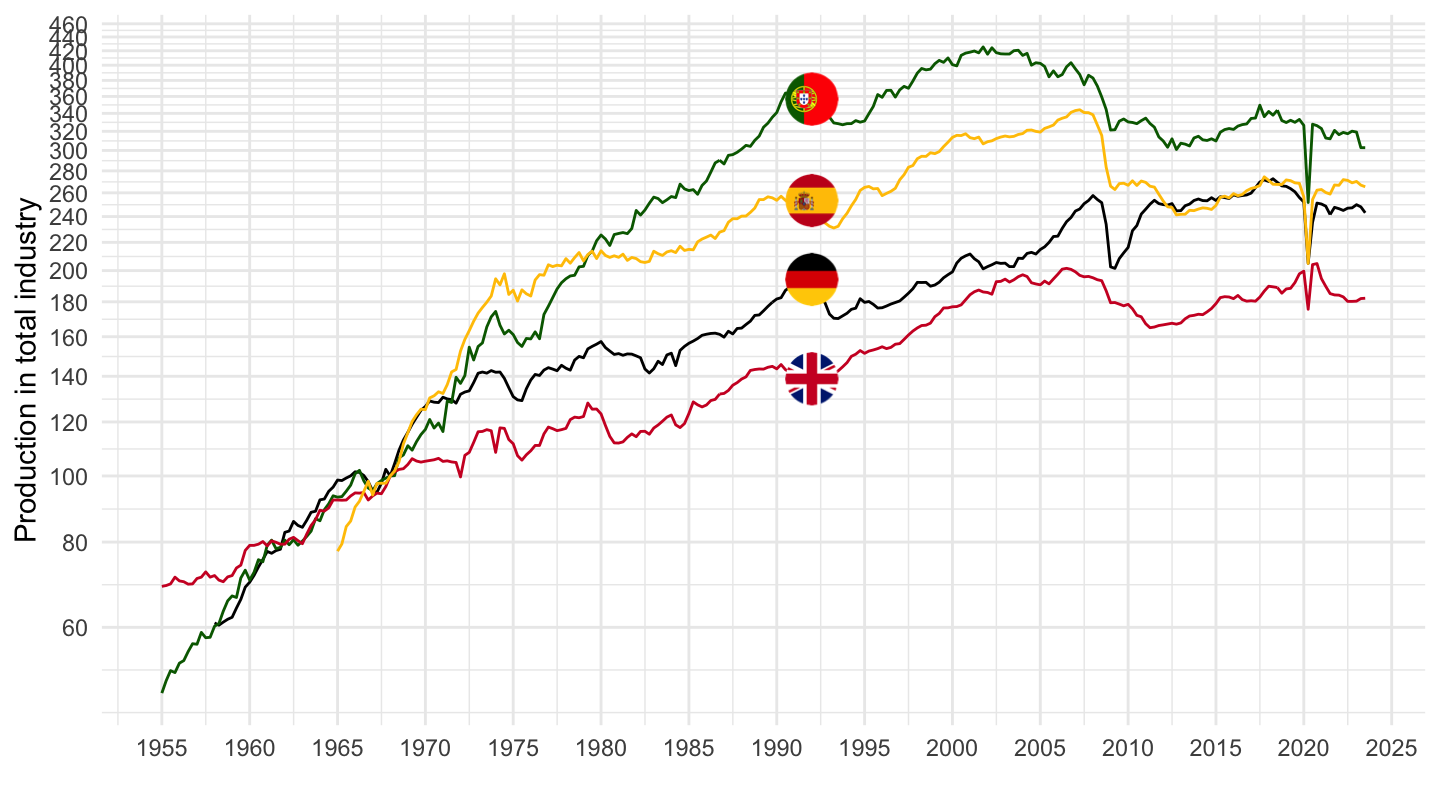
Germany, France, Greece, US
MEI_REAL %>%
  left_join(MEI_REAL_var$LOCATION, by = "LOCATION") %>%
  filter(SUBJECT == "PRINTO01",
         FREQUENCY == "Q",
         LOCATION %in% c("DEU", "FRA", "GRC", "USA")) %>%
  quarter_to_date %>%
  filter(date >= as.Date("1955-01-01")) %>%
  group_by(Location) %>%
  mutate(obsValue = 100*obsValue/obsValue[date == as.Date("1968-01-01")]) %>%
  left_join(colors, by = c("Location" = "country")) %>%
  ggplot(.) + geom_line(aes(x = date, y = obsValue, color = color)) +
  scale_color_identity() + add_4flags +
  theme_minimal() + xlab("") + ylab("Production in total industry") +
  scale_x_date(breaks = seq(1910, 2100, 5) %>% paste0("-01-01") %>% as.Date,
               labels = date_format("%Y")) +
  scale_y_log10(breaks = seq(0, 600, 20),
                     labels = dollar_format(accuracy = 1, prefix = "")) +
  theme(legend.position = c(0.2, 0.80),
        legend.title = element_blank())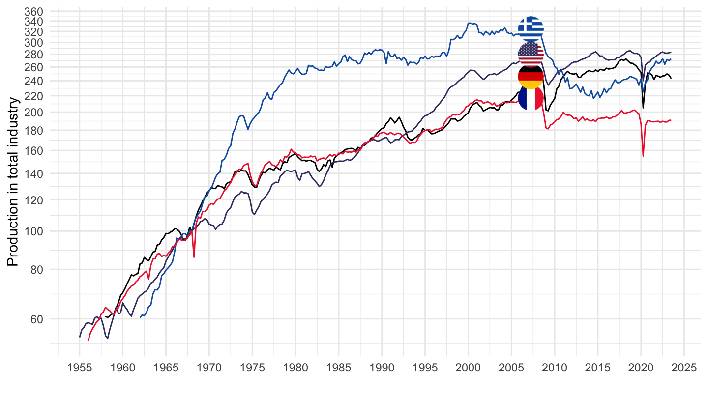
Total retail trade (Volume) sa, Index - SLRTTO01
France, Germany, Italy, United States
Monthly
All
MEI_REAL %>%
  left_join(MEI_REAL_var$LOCATION, by = "LOCATION") %>%
  filter(SUBJECT == "SLRTTO01",
         FREQUENCY == "M",
         LOCATION %in% c("FRA", "DEU", "ITA", "USA")) %>%
  month_to_date %>%
  group_by(Location) %>%
  mutate(obsValue = 100*obsValue/obsValue[date == as.Date("1994-01-01")]) %>%
  left_join(colors, by = c("Location" = "country")) %>%
  ggplot(.) + geom_line(aes(x = date, y = obsValue, color = color)) +
  scale_color_identity() + add_4flags +
  theme_minimal() + xlab("") + ylab("Total retail trade (Volume) sa") +
  scale_x_date(breaks = seq(1910, 2100, 5) %>% paste0("-01-01") %>% as.Date,
               labels = date_format("%Y")) +
  scale_y_log10(breaks = seq(-10, 300, 10),
                     labels = dollar_format(accuracy = 1, prefix = "")) +
  theme(legend.position = c(0.2, 0.80),
        legend.title = element_blank())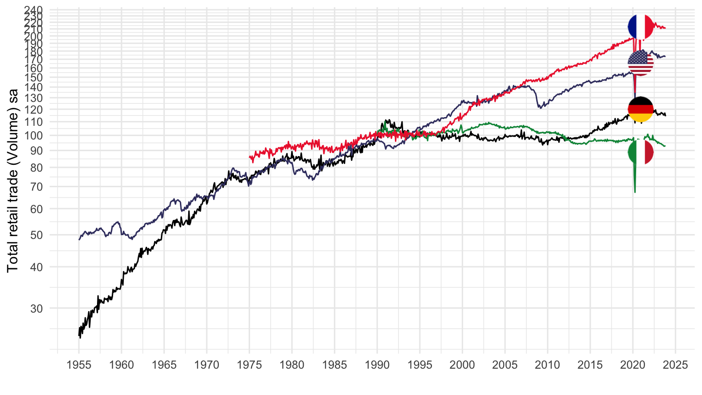
1975-
MEI_REAL %>%
  left_join(MEI_REAL_var$LOCATION, by = "LOCATION") %>%
  filter(SUBJECT == "SLRTTO01",
         FREQUENCY == "M",
         LOCATION %in% c("FRA", "DEU", "ITA", "USA")) %>%
  month_to_date %>%
  filter(date >= as.Date("1975-01-01")) %>%
  group_by(Location) %>%
  mutate(obsValue = 100*obsValue/obsValue[date == as.Date("1994-01-01")]) %>%
  left_join(colors, by = c("Location" = "country")) %>%
  ggplot(.) + geom_line(aes(x = date, y = obsValue, color = color)) +
  scale_color_identity() + add_4flags +
  theme_minimal() + xlab("") + ylab("Total retail trade (Volume) sa") +
  scale_x_date(breaks = seq(1910, 2100, 5) %>% paste0("-01-01") %>% as.Date,
               labels = date_format("%Y")) +
  scale_y_log10(breaks = seq(-10, 300, 10),
                     labels = dollar_format(accuracy = 1, prefix = "")) +
  theme(legend.position = c(0.2, 0.80),
        legend.title = element_blank())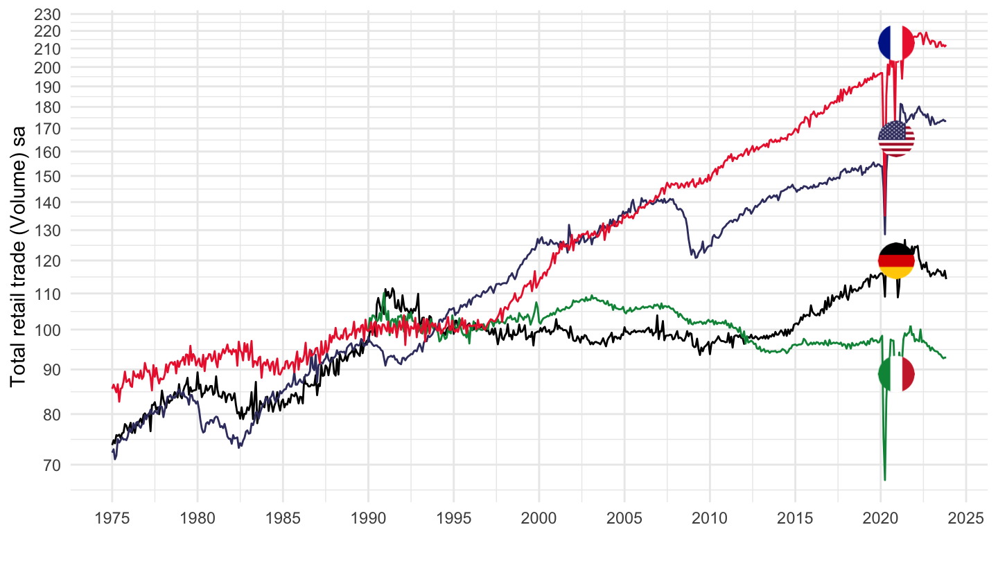
1990-
MEI_REAL %>%
  left_join(MEI_REAL_var$LOCATION, by = "LOCATION") %>%
  filter(SUBJECT == "SLRTTO01",
         FREQUENCY == "M",
         LOCATION %in% c("FRA", "DEU", "ITA", "USA")) %>%
  month_to_date %>%
  filter(date >= as.Date("1990-01-01")) %>%
  group_by(Location) %>%
  mutate(obsValue = 100*obsValue/obsValue[date == as.Date("1994-01-01")]) %>%
  left_join(colors, by = c("Location" = "country")) %>%
  ggplot(.) + geom_line(aes(x = date, y = obsValue, color = color)) +
  scale_color_identity() + add_4flags +
  theme_minimal() + xlab("") + ylab("Total retail trade (Volume) sa") +
  scale_x_date(breaks = seq(1910, 2100, 5) %>% paste0("-01-01") %>% as.Date,
               labels = date_format("%Y")) +
  scale_y_log10(breaks = seq(-10, 300, 10),
                     labels = dollar_format(accuracy = 1, prefix = "")) +
  theme(legend.position = c(0.2, 0.80),
        legend.title = element_blank())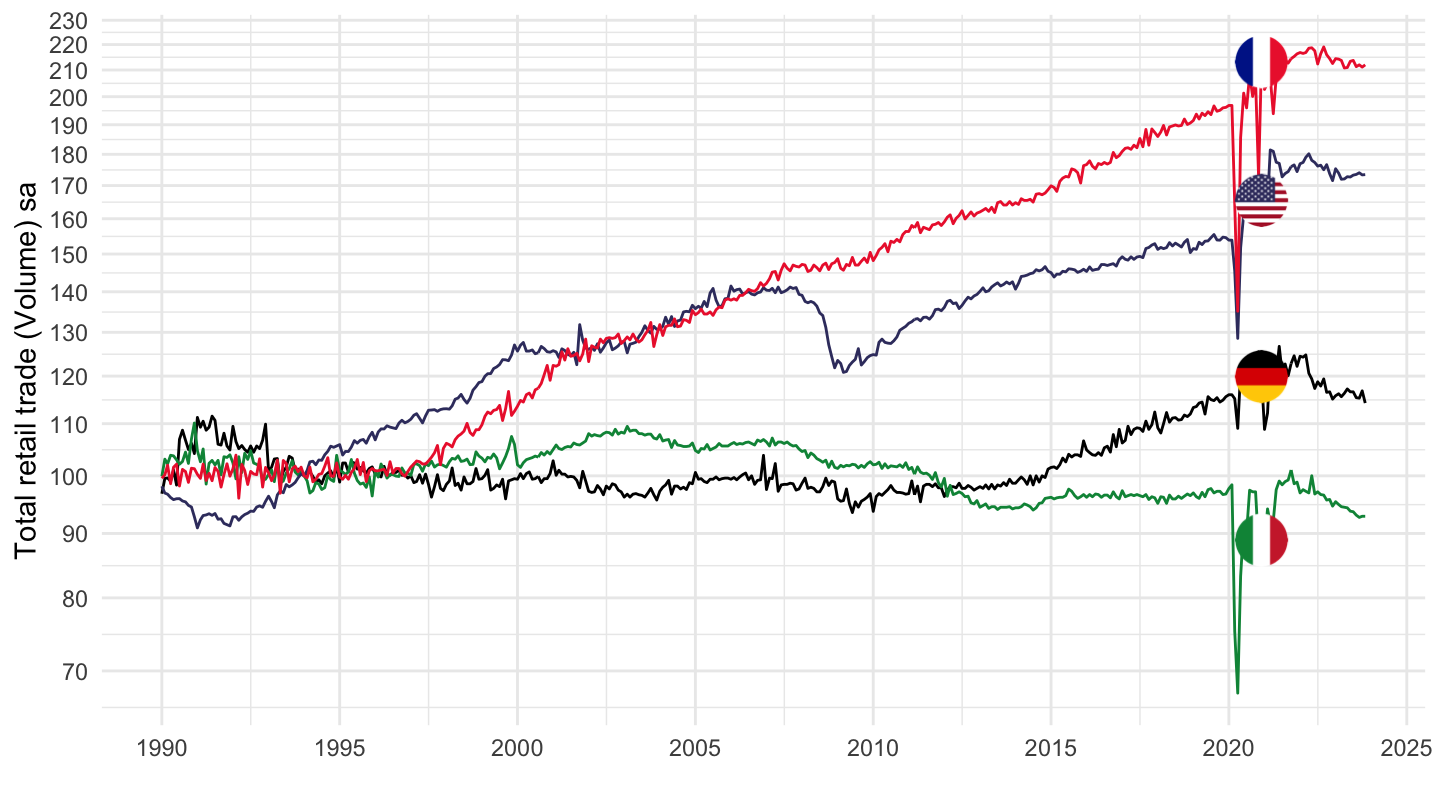
2000-
MEI_REAL %>%
  left_join(MEI_REAL_var$LOCATION, by = "LOCATION") %>%
  filter(SUBJECT == "SLRTTO01",
         FREQUENCY == "M",
         LOCATION %in% c("FRA", "DEU", "ITA", "USA")) %>%
  month_to_date %>%
  filter(date >= as.Date("2000-01-01")) %>%
  group_by(Location) %>%
  mutate(obsValue = 100*obsValue/obsValue[date == as.Date("2000-01-01")]) %>%
  left_join(colors, by = c("Location" = "country")) %>%
  ggplot(.) + geom_line(aes(x = date, y = obsValue, color = color)) +
  scale_color_identity() + add_4flags +
  theme_minimal() + xlab("") + ylab("Total retail trade (Volume) sa") +
  scale_x_date(breaks = seq(1910, 2100, 5) %>% paste0("-01-01") %>% as.Date,
               labels = date_format("%Y")) +
  scale_y_log10(breaks = seq(-10, 300, 10),
                     labels = dollar_format(accuracy = 1, prefix = "")) +
  theme(legend.position = c(0.2, 0.80),
        legend.title = element_blank())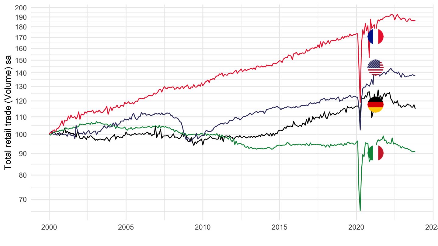
DEU, PRT, ESP, GBR - Monthly
MEI_REAL %>%
  left_join(MEI_REAL_var$LOCATION, by = "LOCATION") %>%
  filter(SUBJECT == "SLRTTO01",
         FREQUENCY == "M",
         LOCATION %in% c("ESP", "PRT", "DEU", "FRA")) %>%
  month_to_date %>%
  filter(date >= as.Date("1990-01-01")) %>%
  select(Location, date, obsValue) %>%
  group_by(Location) %>%
  mutate(obsValue = 100*obsValue/obsValue[date == as.Date("1995-01-01")]) %>%
  left_join(colors, by = c("Location" = "country")) %>%
  ggplot(.) + geom_line(aes(x = date, y = obsValue, color = color)) +
  scale_color_identity() + add_4flags +
  theme_minimal() + xlab("") + ylab("Total retail trade (Volume) sa") +
  scale_x_date(breaks = seq(1910, 2100, 5) %>% paste0("-01-01") %>% as.Date,
               labels = date_format("%Y")) +
  scale_y_log10(breaks = seq(-10, 300, 10),
                     labels = dollar_format(accuracy = 1, prefix = "")) +
  theme(legend.position = c(0.2, 0.80),
        legend.title = element_blank())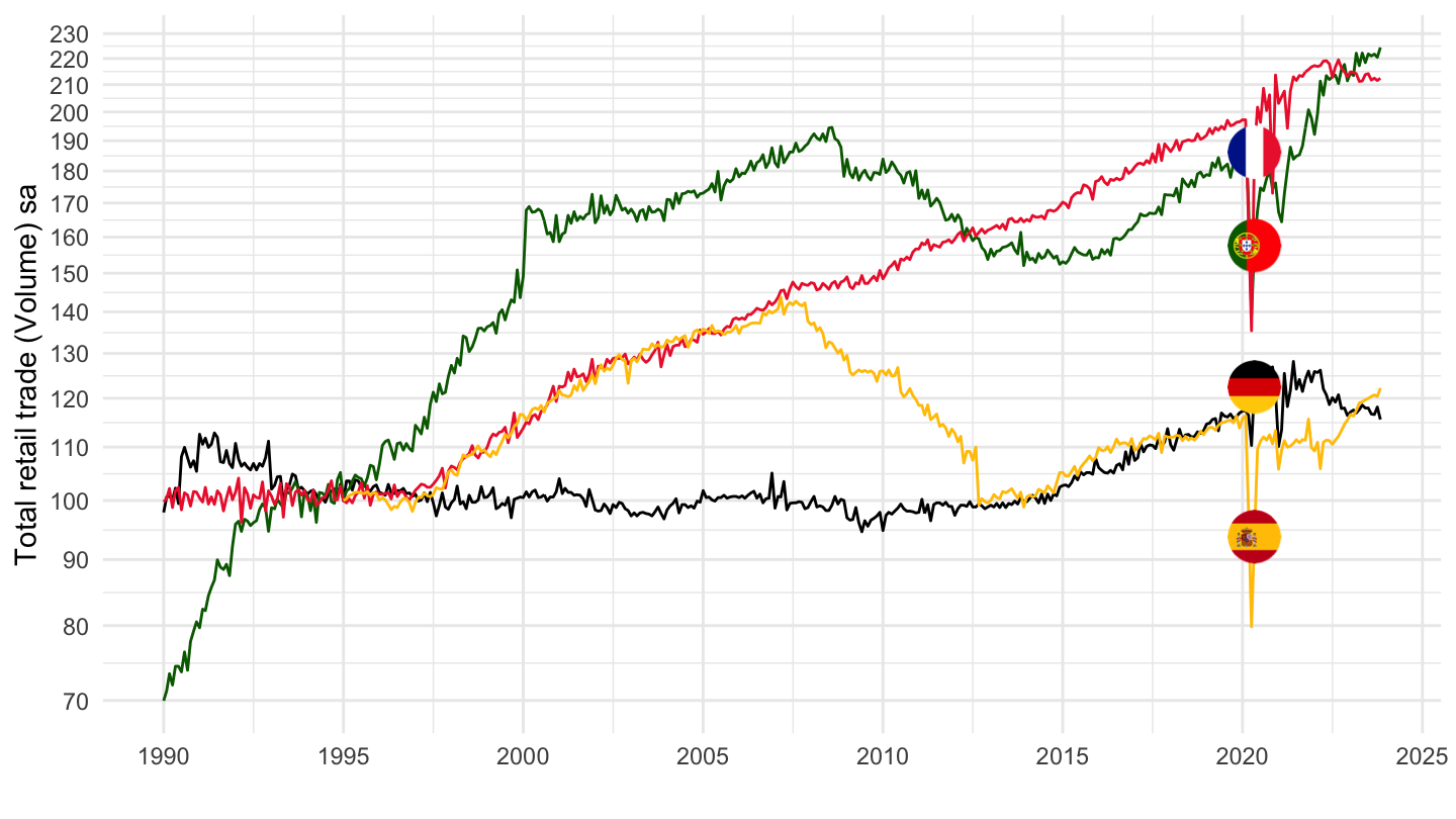
PRMNIG01 - Production of total manufactured intermediate goods sa, Index
France, Germany, Italy, United States
Quarterly
MEI_REAL %>%
  left_join(MEI_REAL_var$LOCATION, by = "LOCATION") %>%
  filter(SUBJECT == "PRMNIG01",
         FREQUENCY == "Q",
         LOCATION %in% c("FRA", "DEU", "ITA", "USA")) %>%
  quarter_to_date %>%
  left_join(colors, by = c("Location" = "country")) %>%
  ggplot(.) + geom_line(aes(x = date, y = obsValue, color = color)) +
  scale_color_identity() + add_4flags +
  theme_minimal() + xlab("") + ylab("Production of total manufactured intermediate goods sa, Index") +
  scale_x_date(breaks = seq(1910, 2100, 5) %>% paste0("-01-01") %>% as.Date,
               labels = date_format("%Y")) +
  scale_y_log10(breaks = seq(-10, 300, 10),
                     labels = dollar_format(accuracy = 1, prefix = "")) +
  theme(legend.position = c(0.2, 0.80),
        legend.title = element_blank())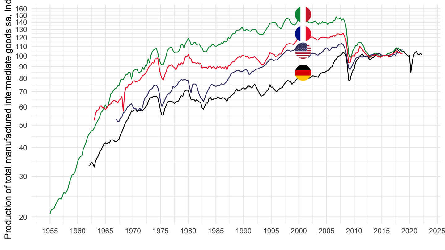
Monthly
All
MEI_REAL %>%
  left_join(MEI_REAL_var$LOCATION, by = "LOCATION") %>%
  filter(SUBJECT == "PRMNIG01",
         FREQUENCY == "M",
         LOCATION %in% c("FRA", "DEU", "ITA", "USA")) %>%
  month_to_date %>%
  left_join(colors, by = c("Location" = "country")) %>%
  ggplot(.) + geom_line(aes(x = date, y = obsValue, color = color)) +
  scale_color_identity() + add_4flags +
  theme_minimal() + xlab("") + ylab("Production of total manufactured intermediate goods sa, Index") +
  scale_x_date(breaks = seq(1910, 2100, 5) %>% paste0("-01-01") %>% as.Date,
               labels = date_format("%Y")) +
  scale_y_log10(breaks = seq(-10, 300, 10),
                     labels = dollar_format(accuracy = 1, prefix = "")) +
  theme(legend.position = c(0.2, 0.80),
        legend.title = element_blank())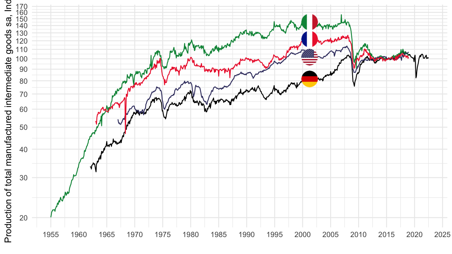
1990-
MEI_REAL %>%
  left_join(MEI_REAL_var$LOCATION, by = "LOCATION") %>%
  filter(SUBJECT == "PRMNIG01",
         FREQUENCY == "M",
         LOCATION %in% c("FRA", "DEU", "ITA", "USA")) %>%
  month_to_date %>%
  filter(date >= as.Date("1990-01-01")) %>%
  group_by(Location) %>%
  mutate(obsValue = 100*obsValue/obsValue[date == as.Date("1994-01-01")]) %>%
  left_join(colors, by = c("Location" = "country")) %>%
  ggplot(.) + geom_line(aes(x = date, y = obsValue, color = color)) +
  scale_color_identity() + add_4flags +
  theme_minimal() + xlab("") + ylab("Production of total manufactured intermediate goods sa, Index") +
  scale_x_date(breaks = seq(1910, 2100, 5) %>% paste0("-01-01") %>% as.Date,
               labels = date_format("%Y")) +
  scale_y_log10(breaks = seq(-10, 300, 10),
                     labels = dollar_format(accuracy = 1, prefix = "")) +
  theme(legend.position = c(0.2, 0.80),
        legend.title = element_blank())