Labour productivity and unit labour costs
Data - Eurostat
Info
Last observation: Quarterly: 2026Q1 (N = 1,307)
First observation: Quarterly: 1980Q1 (N = 24)
Last data update: 23 jul 2026, 22:12. Last compile: 24 jul 2026, 03:03
Structure
Info
Eurostat. Unit labour cost (ULC) measures the average cost of labour per unit of output. It is calculated as the ratio of labour costs to labour productivity. ULC represents a link between productivity and the cost of labour in producing output. Input data are obtained through official transmissions of national accounts’ country data in the European system of accounts - ESA 2010 - transmission programme. Nominal ULC (NULC) is calculated as: [ D1 / EEM] / [ B1GQ / ETO], where: D1 = Compensation of employees, all industries, in current prices EEM = Employees, all industries, in persons (following the domestic concept) B1GQ = Gross domestic product at market prices in millions, chain-linked volumes ETO = Total employment, all industries, in persons (following the domestic concept).
BLS. Unit Labor Cost (ULC) is how much a business pays its workers to produce one unit of output. Businesses pay workers compensation that can include both wages and benefits, such as health insurance and retirement contributions.
https://www.bls.gov/k12/productivity-101/content/what-is-productivity/what-is-unit-labor-cost.htm
na_item: France, Germany, Italy
2022Q2
Code
namq_10_lp_ulc %>%
  filter(geo %in% c("FR", "DE", "IT"),
         time == "2022Q2") %>%
  quarter_to_date %>%


  select(s_adj, na_item, Na_item, values, unit, Unit, Geo) %>%
  spread(Geo, values) %>%
  {if (is_html_output()) datatable(., filter = 'top', rownames = F) else .}
2022Q3
Code
namq_10_lp_ulc %>%
  filter(geo %in% c("FR", "DE", "IT"),
         time == "2022Q3") %>%
  quarter_to_date %>%


  select(s_adj, na_item, Na_item, values, unit, Unit, Geo) %>%
  spread(Geo, values) %>%
  {if (is_html_output()) datatable(., filter = 'top', rownames = F) else .}
2022Q4
Code
namq_10_lp_ulc %>%
  filter(geo %in% c("FR", "DE", "IT"),
         time == "2022Q4") %>%
  quarter_to_date %>%


  select(s_adj, na_item, Na_item, values, unit, Unit, Geo) %>%
  spread(Geo, values) %>%
  {if (is_html_output()) datatable(., filter = 'top', rownames = F) else .}
RLPR_HW - Real labour productivity per hour worked
France, Germany, Italy
All
Code
namq_10_lp_ulc %>%
  filter(geo %in% c("FR", "DE", "IT"),
         na_item == "RLPR_HW",
         unit == "I15",
         s_adj == "SCA") %>%
  quarter_to_date %>%

  left_join(colors, by = c("Geo" = "country")) %>%
  ggplot + theme_minimal() + xlab("") + ylab("") +
  geom_line(aes(x = date, y = values, color = color)) +
  scale_color_identity() + add_3flags +
  theme(legend.position = c(0.3, 0.85),
        legend.title = element_blank()) +
  scale_x_date(breaks = as.Date(paste0(seq(1960, 2100, 2), "-01-01")),
               labels = date_format("%Y")) +
  scale_y_continuous(breaks = seq(0, 200, 10),
                     labels = scales::dollar_format(su = "", p = ""))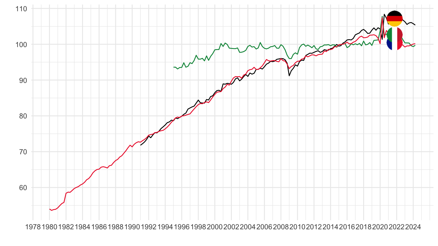
1995-
Code
namq_10_lp_ulc %>%
  filter(geo %in% c("FR", "DE", "IT"),
         na_item == "RLPR_HW",
         unit == "I15",
         s_adj == "SCA") %>%
  quarter_to_date %>%
  filter(date >= as.Date("1995-01-01")) %>%

  left_join(colors, by = c("Geo" = "country")) %>%
  ggplot + theme_minimal() + xlab("") + ylab("") +
  geom_line(aes(x = date, y = values, color = color)) +
  scale_color_identity() + add_3flags +
  theme(legend.position = c(0.3, 0.85),
        legend.title = element_blank()) +
  scale_x_date(breaks = as.Date(paste0(seq(1960, 2100, 2), "-01-01")),
               labels = date_format("%Y")) +
  scale_y_continuous(breaks = seq(0, 200, 5),
                     labels = scales::dollar_format(su = "", p = ""))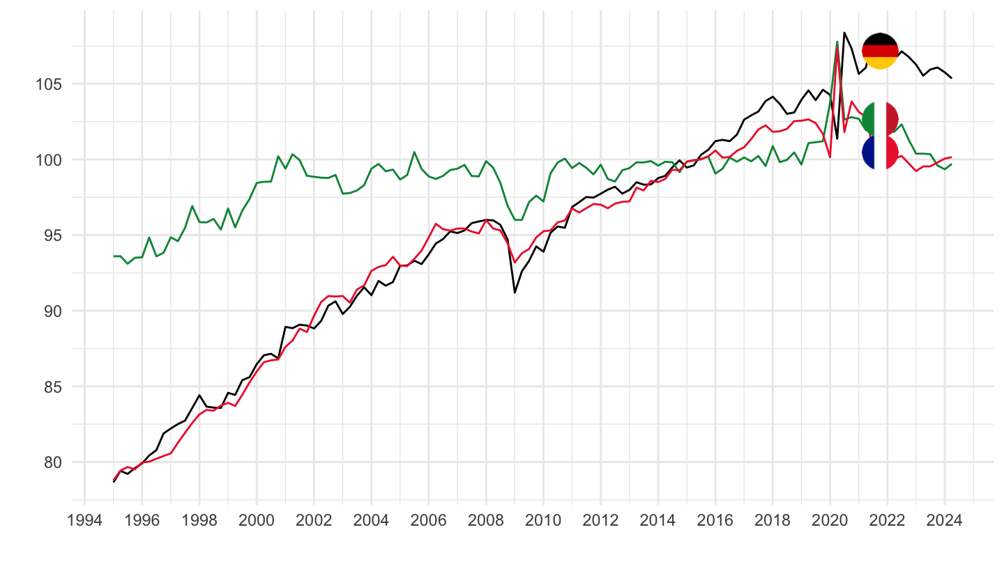
1996-
Code
namq_10_lp_ulc %>%
  filter(geo %in% c("FR", "DE", "IT"),
         na_item == "RLPR_HW",
         unit == "I15",
         s_adj == "SCA") %>%
  quarter_to_date %>%
  filter(date >= as.Date("1996-01-01")) %>%

  left_join(colors, by = c("Geo" = "country")) %>%
  group_by(geo) %>%
  mutate(values = 100*values/ values[date == as.Date("1996-01-01")]) %>%
  ggplot + theme_minimal() + xlab("") + ylab("") +
  geom_line(aes(x = date, y = values, color = color)) +
  scale_color_identity() + add_3flags +
  theme(legend.position = c(0.3, 0.85),
        legend.title = element_blank()) +
  scale_x_date(breaks = as.Date(paste0(seq(1960, 2100, 2), "-01-01")),
               labels = date_format("%Y")) +
  scale_y_log10(breaks = seq(0, 200, 5),
                     labels = scales::dollar_format(su = "", p = "", acc = 1))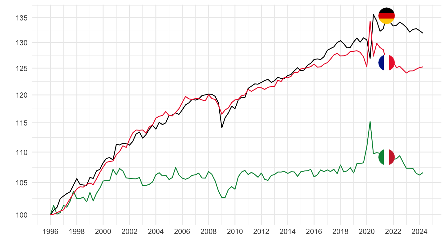
2010-
Code
namq_10_lp_ulc %>%
  filter(geo %in% c("FR", "DE", "IT"),
         na_item == "RLPR_HW",
         unit == "I15",
         s_adj == "SCA") %>%
  quarter_to_date %>%
  filter(date >= as.Date("2010-01-01")) %>%

  left_join(colors, by = c("Geo" = "country")) %>%
  ggplot + theme_minimal() + xlab("") + ylab("") +
  geom_line(aes(x = date, y = values, color = color)) +
  scale_color_identity() + add_3flags +
  theme(legend.position = c(0.3, 0.85),
        legend.title = element_blank()) +
  scale_x_date(breaks = as.Date(paste0(seq(1960, 2100, 2), "-01-01")),
               labels = date_format("%Y")) +
  scale_y_continuous(breaks = seq(0, 200, 2),
                     labels = scales::dollar_format(su = "", p = ""))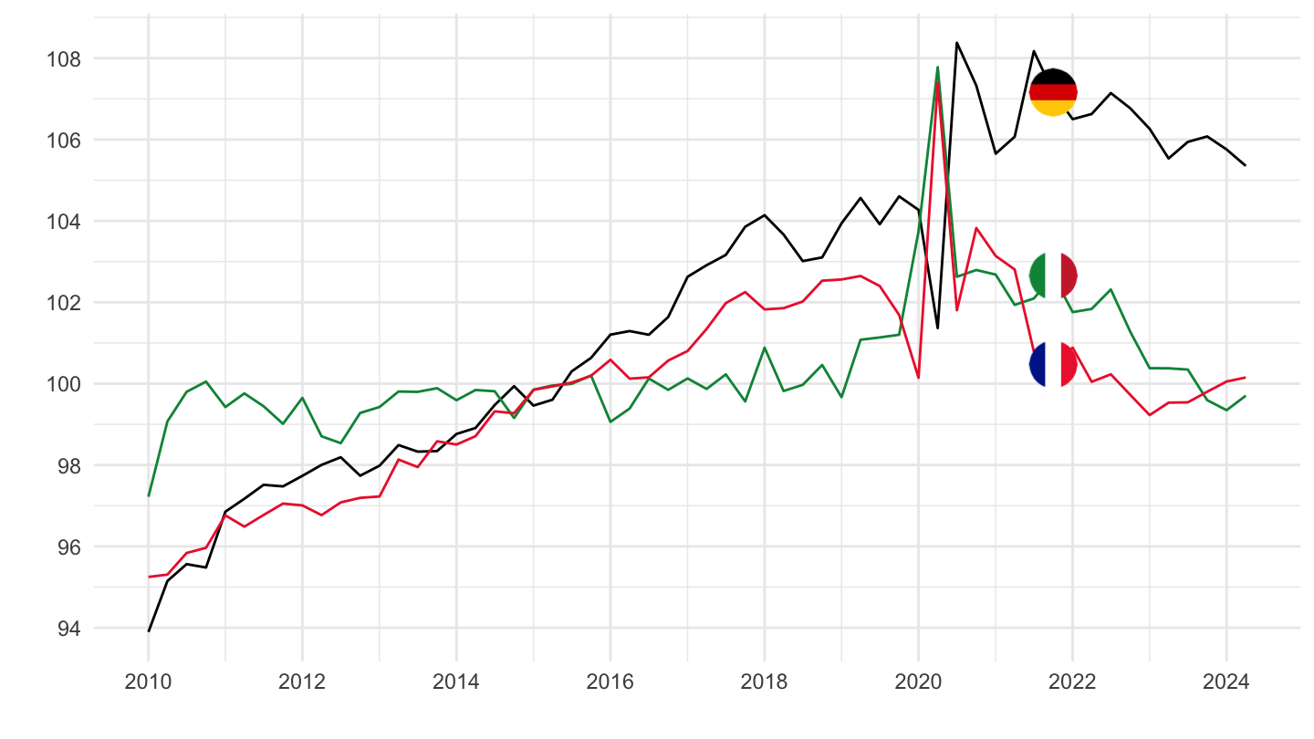
RLPR_PER - Real labour productivity per person
France, Germany, Italy
All
Code
namq_10_lp_ulc %>%
  filter(geo %in% c("FR", "DE", "IT"),
         na_item == "RLPR_PER",
         unit == "I15",
         s_adj == "SCA") %>%
  quarter_to_date %>%

  left_join(colors, by = c("Geo" = "country")) %>%
  ggplot + theme_minimal() + xlab("") + ylab("") +
  geom_line(aes(x = date, y = values, color = color)) +
  scale_color_identity() + add_3flags +
  theme(legend.position = c(0.3, 0.85),
        legend.title = element_blank()) +
  scale_x_date(breaks = as.Date(paste0(seq(1960, 2100, 2), "-01-01")),
               labels = date_format("%Y")) +
  scale_y_continuous(breaks = seq(0, 200, 10),
                     labels = scales::dollar_format(su = "", p = ""))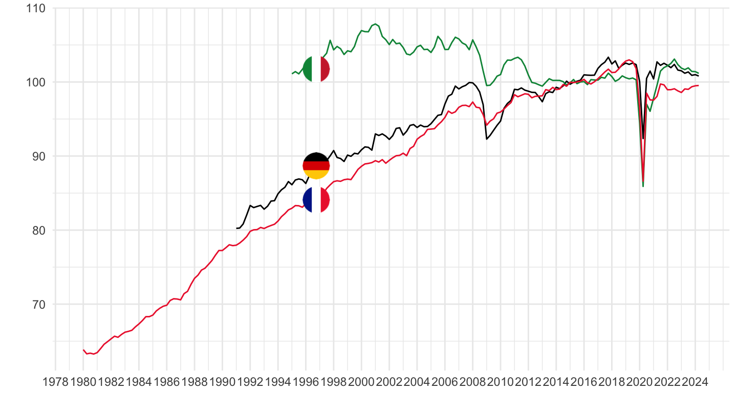
1995-
Code
namq_10_lp_ulc %>%
  filter(geo %in% c("FR", "DE", "IT"),
         na_item == "RLPR_PER",
         unit == "I15",
         s_adj == "SCA") %>%
  quarter_to_date %>%
  filter(date >= as.Date("1995-01-01")) %>%

  left_join(colors, by = c("Geo" = "country")) %>%
  ggplot + theme_minimal() + xlab("") + ylab("") +
  geom_line(aes(x = date, y = values, color = color)) +
  scale_color_identity() + add_3flags +
  theme(legend.position = c(0.3, 0.85),
        legend.title = element_blank()) +
  scale_x_date(breaks = as.Date(paste0(seq(1960, 2100, 2), "-01-01")),
               labels = date_format("%Y")) +
  scale_y_continuous(breaks = seq(0, 200, 5),
                     labels = scales::dollar_format(su = "", p = ""))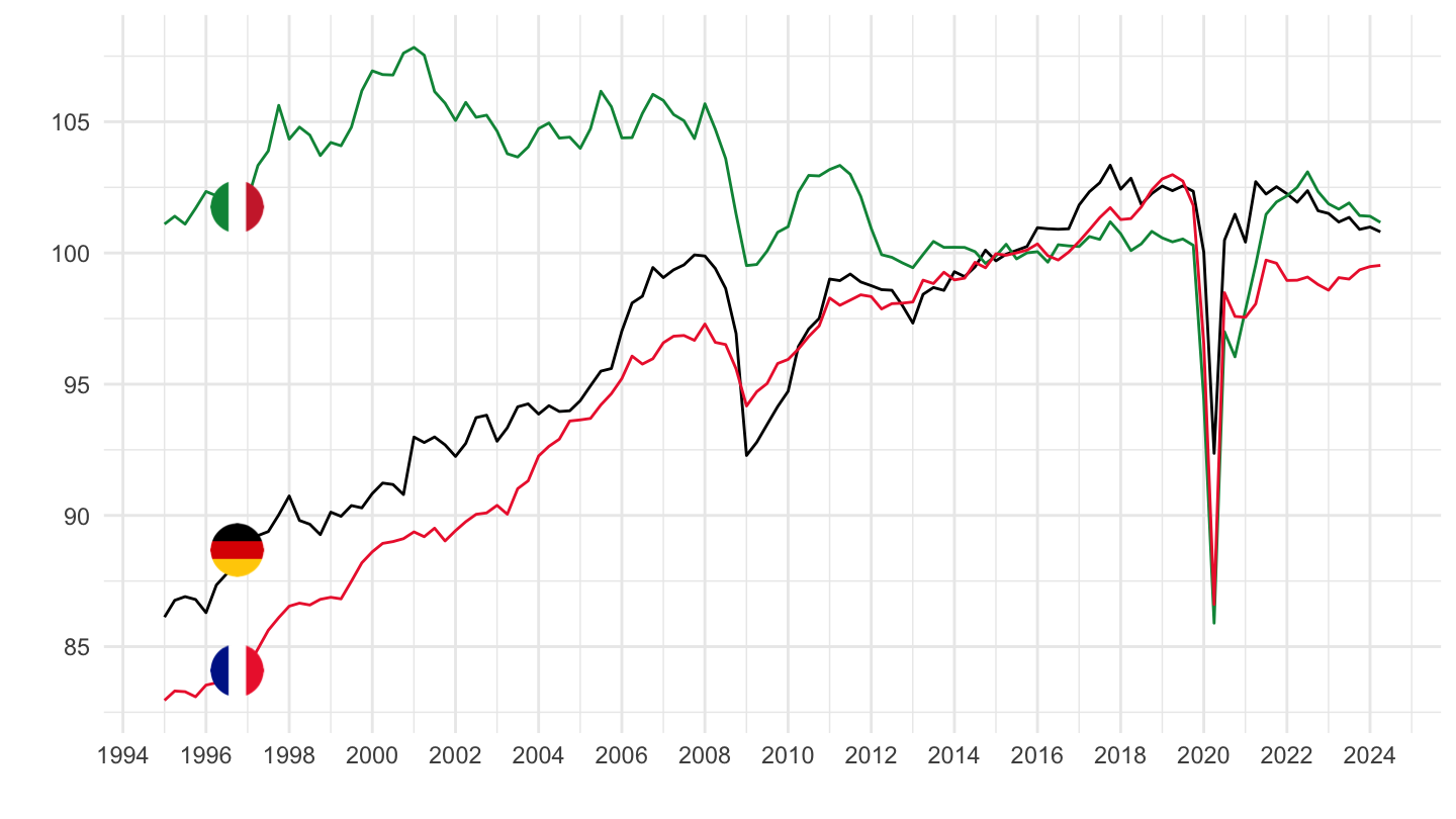
1996-
Code
namq_10_lp_ulc %>%
  filter(geo %in% c("FR", "DE", "IT"),
         na_item == "RLPR_PER",
         unit == "I15",
         s_adj == "SCA") %>%
  quarter_to_date %>%
  filter(date >= as.Date("1996-01-01")) %>%

  left_join(colors, by = c("Geo" = "country")) %>%
  group_by(geo) %>%
  mutate(values = 100*values/ values[date == as.Date("1996-01-01")]) %>%
  ggplot + theme_minimal() + xlab("") + ylab("") +
  geom_line(aes(x = date, y = values, color = color)) +
  scale_color_identity() + add_3flags +
  theme(legend.position = c(0.3, 0.85),
        legend.title = element_blank()) +
  scale_x_date(breaks = as.Date(paste0(seq(1960, 2100, 2), "-01-01")),
               labels = date_format("%Y")) +
  scale_y_log10(breaks = seq(0, 200, 5),
                     labels = scales::dollar_format(su = "", p = "", acc = 1))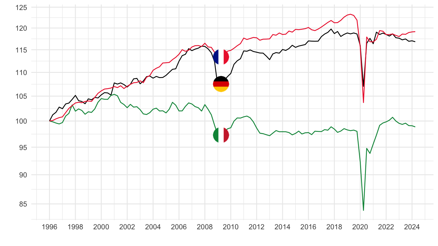
2010-
Code
namq_10_lp_ulc %>%
  filter(geo %in% c("FR", "DE", "IT"),
         na_item == "RLPR_PER",
         unit == "I15",
         s_adj == "SCA") %>%
  quarter_to_date %>%
  filter(date >= as.Date("2010-01-01")) %>%

  left_join(colors, by = c("Geo" = "country")) %>%
  ggplot + theme_minimal() + xlab("") + ylab("") +
  geom_line(aes(x = date, y = values, color = color)) +
  scale_color_identity() + add_3flags +
  theme(legend.position = c(0.3, 0.85),
        legend.title = element_blank()) +
  scale_x_date(breaks = as.Date(paste0(seq(1960, 2100, 2), "-01-01")),
               labels = date_format("%Y")) +
  scale_y_continuous(breaks = seq(0, 200, 2),
                     labels = scales::dollar_format(su = "", p = ""))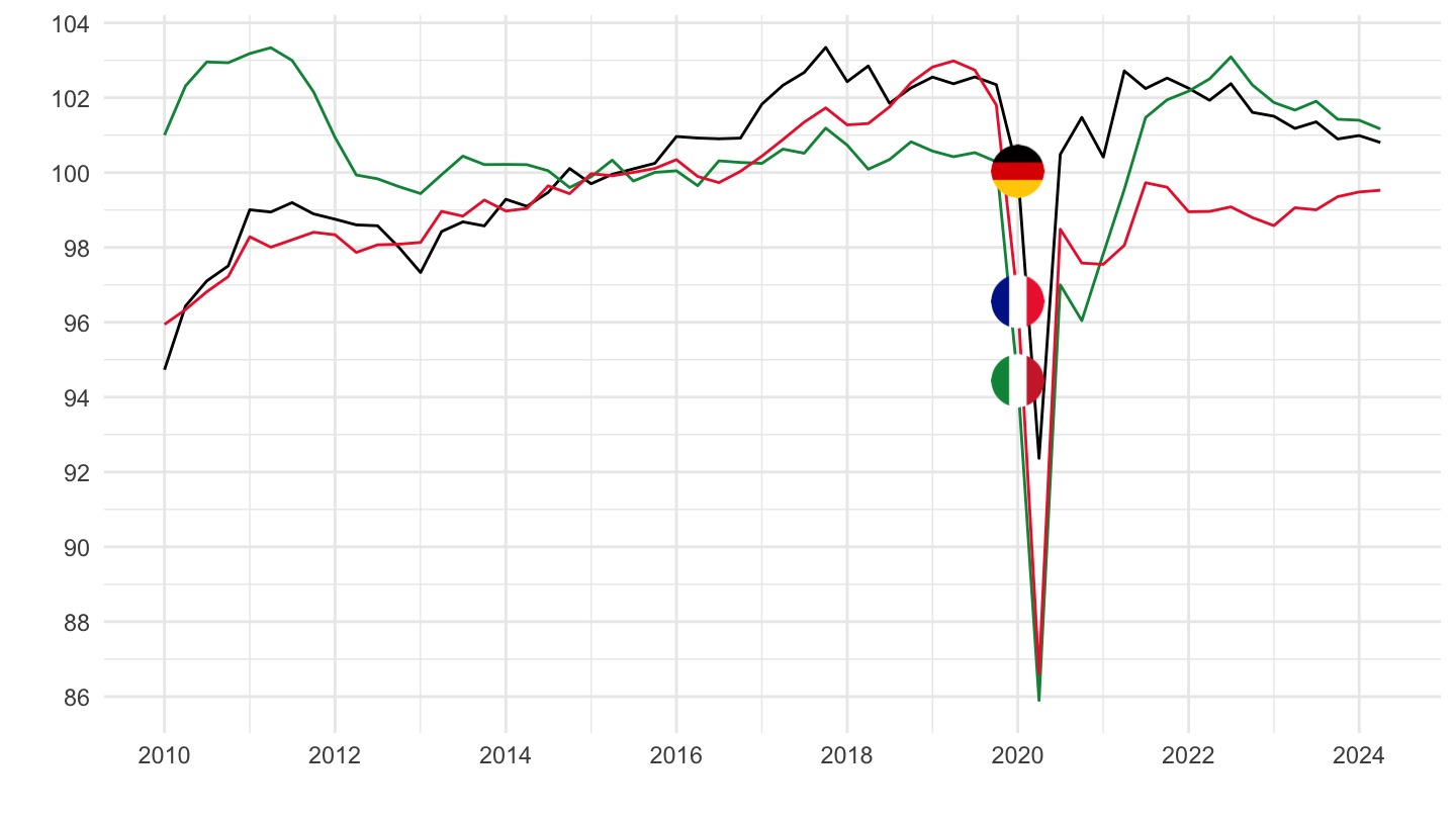
NULC_PER - Nominal unit labour cost based on persons
Greece, Spain, Portugal
Code
namq_10_lp_ulc %>%
  filter(geo %in% c("EL", "ES", "PT"),
         na_item == "NULC_PER",
         unit == "I15",
         s_adj == "NSA") %>%
  quarter_to_date %>%

  left_join(colors, by = c("Geo" = "country")) %>%
  ggplot + theme_minimal() + xlab("") + ylab("Nominal unit labour cost based on persons") +
  geom_line(aes(x = date, y = values, color = color)) +
  scale_color_identity() + add_3flags +
  theme(legend.position = c(0.3, 0.85),
        legend.title = element_blank()) +
  scale_x_date(breaks = as.Date(paste0(seq(1960, 2100, 2), "-01-01")),
               labels = date_format("%Y")) +
  scale_y_continuous(breaks = seq(0, 200, 10),
                     labels = scales::dollar_format(su = "", p = ""))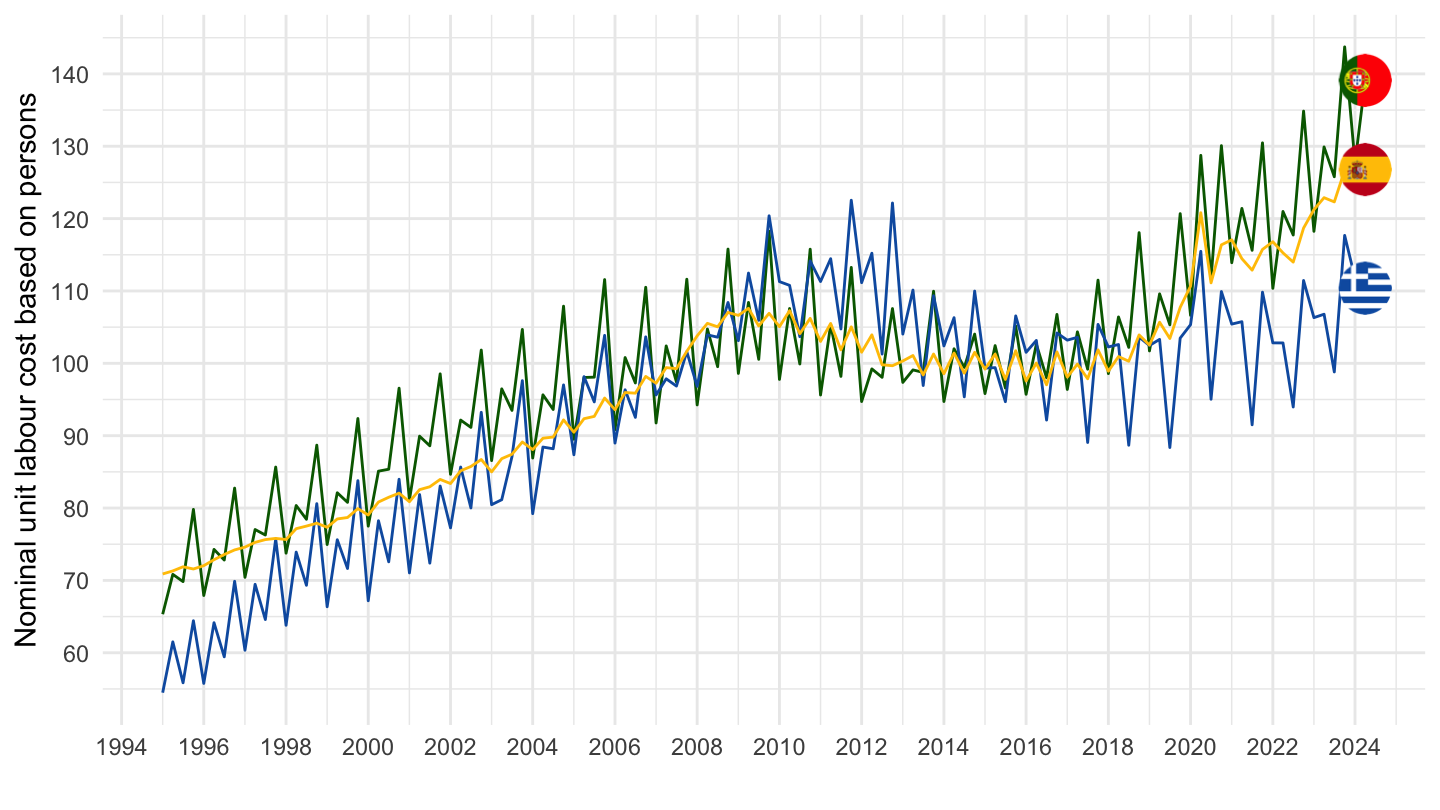
France, Germany, Italy
Code
namq_10_lp_ulc %>%
  filter(geo %in% c("FR", "DE", "IT"),
         na_item == "NULC_PER",
         unit == "I15",
         s_adj == "NSA") %>%
  quarter_to_date %>%

  left_join(colors, by = c("Geo" = "country")) %>%
  ggplot + theme_minimal() + xlab("") + ylab("Nominal unit labour cost based on persons") +
  geom_line(aes(x = date, y = values, color = color)) +
  scale_color_identity() + add_3flags +
  theme(legend.position = c(0.3, 0.85),
        legend.title = element_blank()) +
  scale_x_date(breaks = as.Date(paste0(seq(1960, 2100, 2), "-01-01")),
               labels = date_format("%Y")) +
  scale_y_continuous(breaks = seq(0, 200, 10),
                     labels = scales::dollar_format(su = "", p = ""))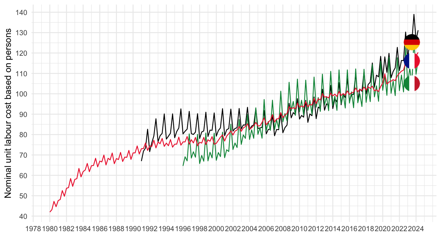
France, Germany
NSA
Code
namq_10_lp_ulc %>%
  filter(geo %in% c("FR", "DE"),
         na_item == "NULC_PER",
         unit == "I15",
         s_adj == "NSA") %>%
  quarter_to_date %>%
  filter(date >= as.Date("1990-01-01")) %>%

  left_join(colors, by = c("Geo" = "country")) %>%
  ggplot + theme_minimal() + xlab("") + ylab("Nominal unit labour cost based on persons") +
  geom_line(aes(x = date, y = values, color = color)) +
  scale_color_identity() + add_2flags +
  theme(legend.position = c(0.3, 0.85),
        legend.title = element_blank()) +
  scale_x_date(breaks = as.Date(paste0(seq(1960, 2100, 2), "-01-01")),
               labels = date_format("%Y")) +
  scale_y_continuous(breaks = seq(0, 200, 5),
                     labels = scales::dollar_format(su = "", p = ""))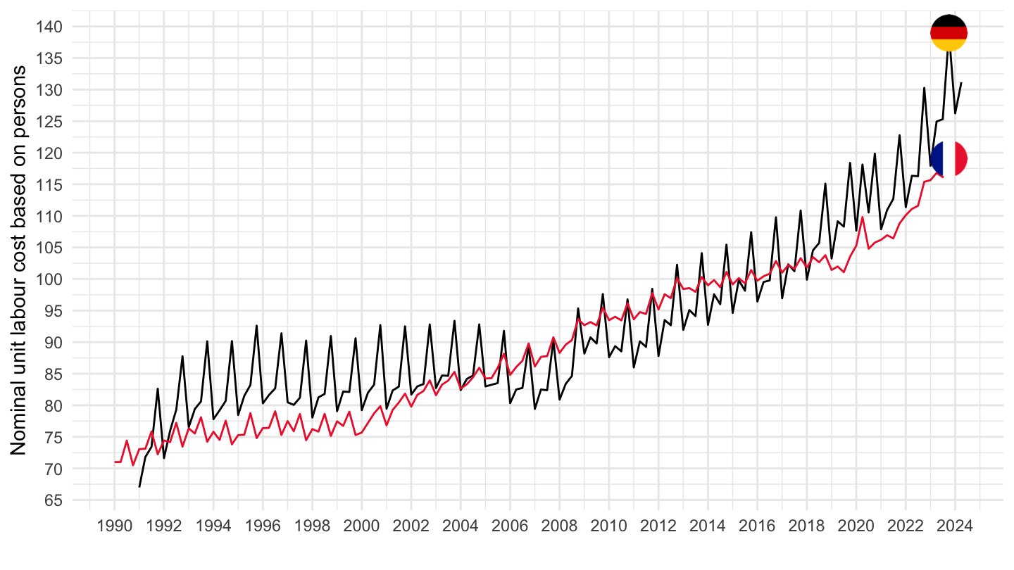
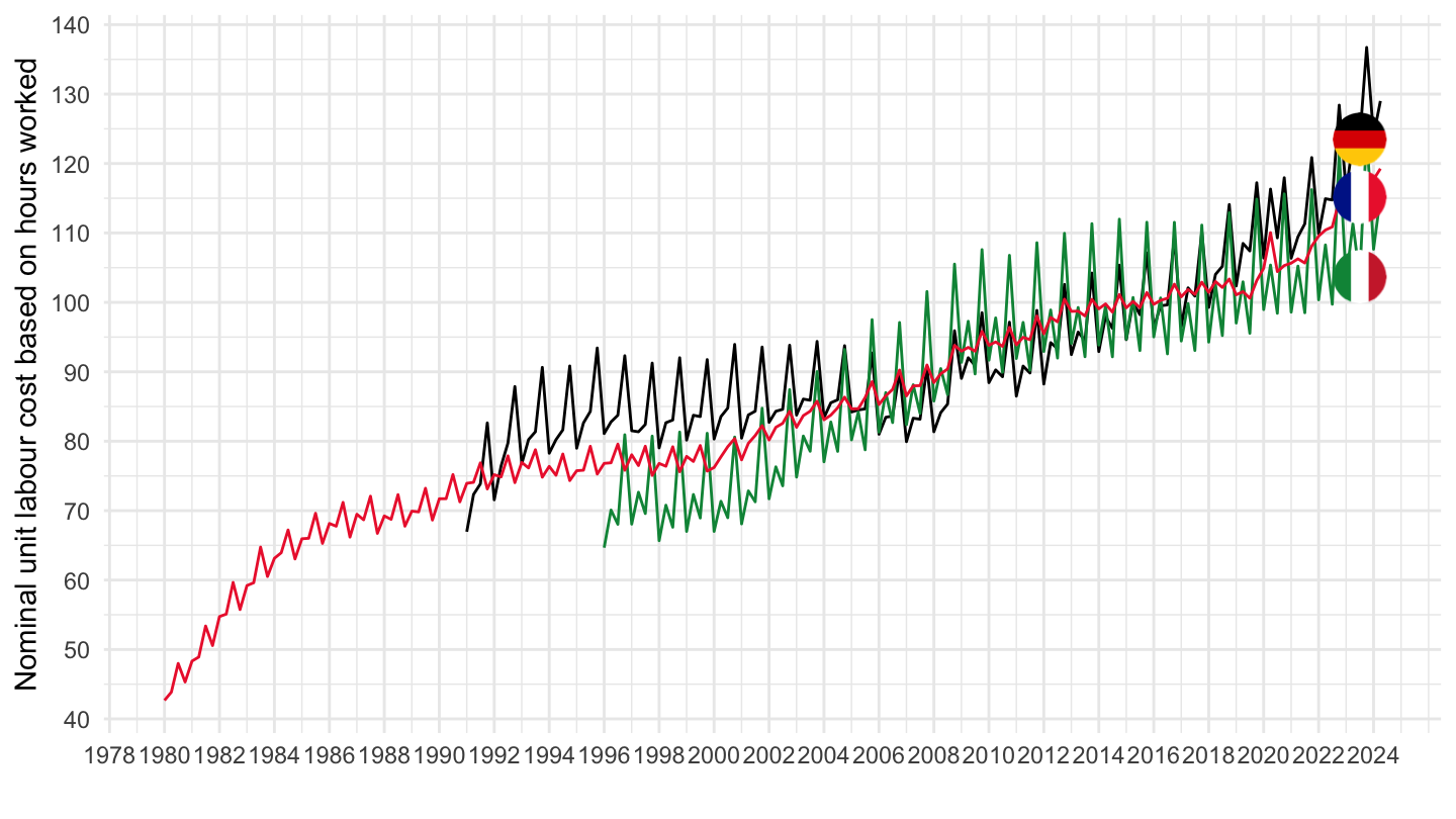
NULC_HW - Nominal unit labour cost based on hours worked
France, Germany, Italy
Code
namq_10_lp_ulc %>%
  filter(geo %in% c("FR", "DE", "IT"),
         na_item == "NULC_HW",
         unit == "I15",
         s_adj == "NSA") %>%
  quarter_to_date %>%

  left_join(colors, by = c("Geo" = "country")) %>%
  ggplot + theme_minimal() + xlab("") + ylab("Nominal unit labour cost based on hours worked") +
  geom_line(aes(x = date, y = values, color = color)) +
  scale_color_identity() + add_3flags +
  theme(legend.position = c(0.3, 0.85),
        legend.title = element_blank()) +
  scale_x_date(breaks = as.Date(paste0(seq(1960, 2100, 2), "-01-01")),
               labels = date_format("%Y")) +
  scale_y_continuous(breaks = seq(0, 200, 10),
                     labels = scales::dollar_format(su = "", p = ""))