
Last observation: 2025 (N = 233)
First observation: 1990 (N = 234)
Last data update: 16 oct. 2026, 00:39
Last compile: 16 oct. 2026, 00:49
NY.GDP.MKTP.PP.CD |>
  left_join(iso2c, by = "iso2c") |>
  group_by(iso2c, Iso2c) |>

  mutate(value = round(value/(10^9))) %>%
  summarise(Nobs = n(),
            `Year 1` = first(year),
            `GDP 1 (Bn)` = first(value) %>% paste0("$ ", .),
            `Year 2` = last(year),
            `GDP 2 (Bn)` = last(value) %>% paste0("$ ", .)) |>
  arrange(-Nobs) |>
  mutate(Flag = gsub(" ", "-", str_to_lower(Iso2c)),
         Flag = paste0('<img src="../../bib/flags/vsmall/', Flag, '.png" alt="Flag">')) |>
  select(Flag, everything()) %>%
{if (is_html_output()) datatable(., filter = 'top', rownames = F, escape = F) else .}NY.GDP.MKTP.PP.CD |>
right_join(iso2c |>
filter((region != "Aggregates") & (region != "NA")),
by = "iso2c") |>
group_by(iso2c, Iso2c) |>
mutate(value = round(value/(10^9))) |>
summarise(`GDP (Bn)` = last(value)) |>
arrange(-`GDP (Bn)`) %>%
mutate(`GDP (Bn)` = `GDP (Bn)` %>% paste0("$ ", ., " Bn")) |>
mutate(Flag = gsub(" ", "-", str_to_lower(Iso2c)),
Flag = paste0('<img src="../../bib/flags/vsmall/', Flag, '.png" alt="Flag">')) |>
select(Flag, everything()) %>%
{if (is_html_output()) datatable(., filter = 'top', rownames = F, escape = F) else .}NY.GDP.MKTP.PP.CD |>
right_join(iso2c, by = "iso2c") |>
group_by(iso2c, Iso2c) |>
mutate(value = round(value/(10^9))) |>
summarise(`GDP (Bn)` = last(value)) |>
arrange(-`GDP (Bn)`) %>%
mutate(`GDP (Bn)` = `GDP (Bn)` %>% paste0("$ ", ., " Bn")) %>%
{if (is_html_output()) datatable(., filter = 'top', rownames = F) else .}NY.GDP.MKTP.PP.CD |>
left_join(iso2c, by = "iso2c") |>
year_to_date() |>
filter(iso2c %in% c("XC", "US"),
date >= as.Date("2008-01-01")) |>
group_by(iso2c) |>
arrange(date) |>
mutate(value = 100*value/value[1]) |>
mutate(Iso2c = ifelse(iso2c == "XC", "Europe", Iso2c)) |>
add_flag_color("Iso2c") |>
ggplot() + theme_minimal() + scale_color_identity() +
geom_line(aes(x = date, y = value, color = color)) +
add_flags +
scale_x_date(breaks = seq(1950, 2100, 2) |> paste0("-01-01") |> as.Date(),
labels = date_format("%Y")) +
scale_y_log10(breaks = seq(70, 300, 5)) +
xlab("") + ylab("PIB en $ (100 = 2008)")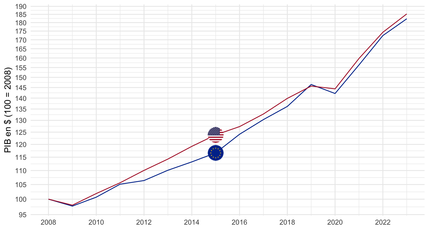
NY.GDP.MKTP.PP.CD |>
  left_join(iso2c, by = "iso2c") |>
  year_to_date() |>
  filter(iso2c %in% c("XC", "US"),
         date >= as.Date("2008-01-01")) |>
  group_by(iso2c) |>
  arrange(date) |>
  mutate(Iso2c = ifelse(iso2c == "XC", "Europe", Iso2c)) |>
  add_flag_color("Iso2c") |>
  ungroup() |>
  mutate(dollar = value/10^9,
         value = 100*value/value[2]) |>
  ggplot() + theme_minimal() + scale_color_identity() +
  geom_line(aes(x = date, y = value, color = color)) +
  add_flags +
  scale_x_date(breaks = seq(1950, 2100, 2) |> paste0("-01-01") |> as.Date(),
               labels = date_format("%Y")) +
  scale_y_log10(breaks = seq(10, 300, 5)) +
  xlab("") + ylab("PIB en $ (100 = Zone Euro, 2008)") +
  geom_text_repel(data = . %>% filter(year(date) %in% seq(2008, 2022, 2)),
                                      aes(x = date, y = value, label = paste0("$", round(dollar, digits = -2), " Md")))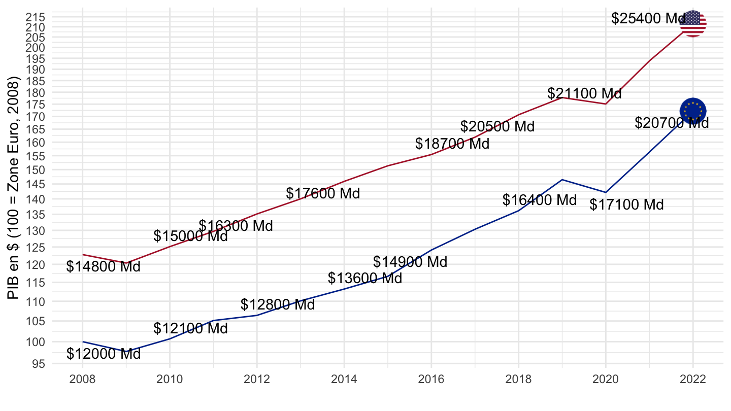
NY.GDP.MKTP.PP.CD |>
  right_join(iso2c, by = "iso2c") |>
  filter(iso2c %in% c("1W", "US", "CN", "EU")) |>
  group_by(year) |>
  mutate(value = value/value[iso2c == "1W"]) |>
  year_to_date() |>
  filter(!(iso2c == "1W")) |>
  mutate(Iso2c = ifelse(iso2c == "EU", "Europe", Iso2c)) |>
  add_flag_color("Iso2c") |>
  ggplot() + theme_minimal() + scale_color_identity() +
  geom_line(aes(x = date, y = value, color = color)) +
  add_flags +
  scale_x_date(breaks = seq(1950, 2100, 5) |> paste0("-01-01") |> as.Date(),
               labels = date_format("%Y")) +
  scale_y_continuous(breaks = 0.01*seq(0, 70, 2),
                     labels = scales::percent_format(accuracy = 1),
                     limits = c(0, 0.23)) +
  xlab("") + ylab("% du PIB mondial en Parité de Pouvoir d'Achat")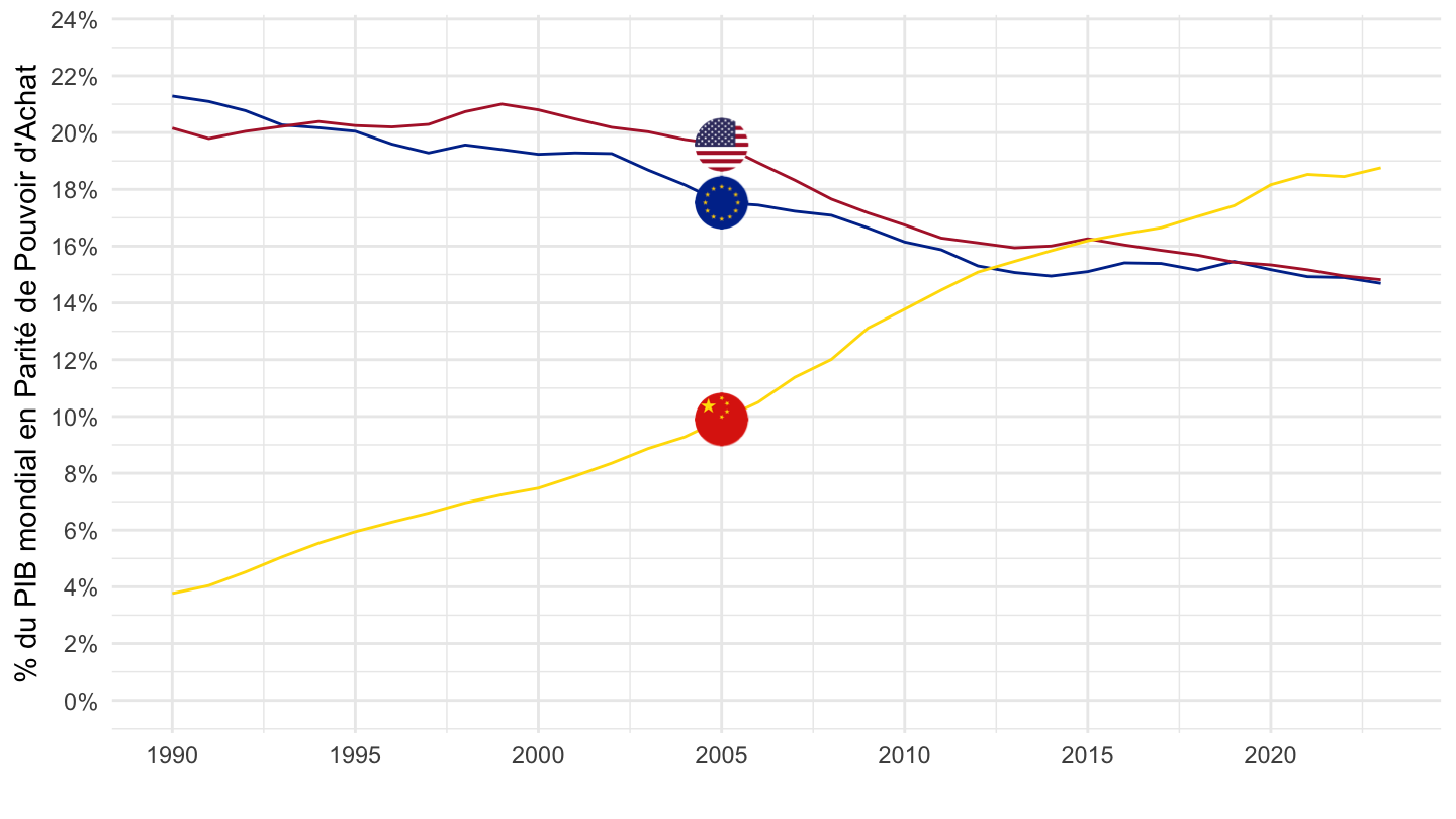
NY.GDP.MKTP.PP.CD |>
  right_join(iso2c, by = "iso2c") |>
  filter(iso2c %in% c("1W", "US", "CN", "EU")) |>
  group_by(year) |>
  mutate(value = value/value[iso2c == "1W"]) |>
  year_to_date() |>
  filter(!(iso2c == "1W")) |>
  mutate(Iso2c = ifelse(iso2c == "EU", "Europe", Iso2c)) |>
  add_flag_color("Iso2c") |>
  ggplot() + theme_minimal() + scale_color_identity() +
  geom_line(aes(x = date, y = value, color = color)) +
  add_flags +
  scale_x_date(breaks = seq(1950, 2100, 5) |> paste0("-01-01") |> as.Date(),
               labels = date_format("%Y")) +
  scale_y_log10(breaks = 0.01*seq(0, 70, 5),
                     labels = scales::percent_format(accuracy = 1)) +
  xlab("") + ylab("% du PIB mondial en Parité de Pouvoir d'Achat")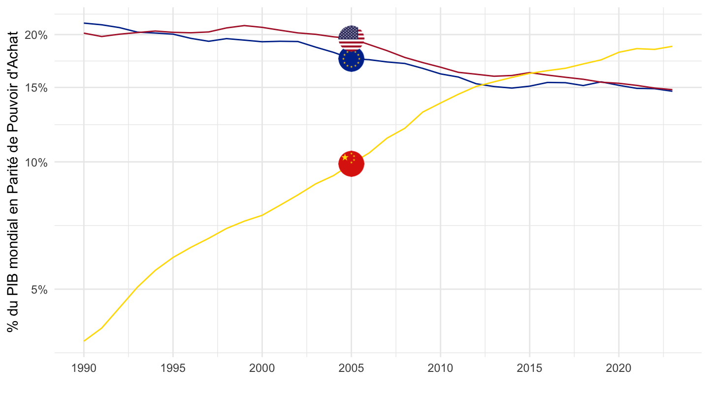
plot1 <- NY.GDP.MKTP.CD |>
  right_join(iso2c, by = "iso2c") |>
  filter(iso2c %in% c("1W", "US", "CN", "EU")) |>
  group_by(year) |>
  filter(n() > 3) |>
  mutate(value = value/value[iso2c == "1W"]) |>
  year_to_date() |>
  filter(!(iso2c == "1W")) |>
  mutate(Iso2c = ifelse(iso2c == "XC", "Europe", Iso2c)) |>
  filter(date >= as.Date("1990-01-01")) |>
  add_flag_color("Iso2c") |>
  ggplot() + theme_minimal() + scale_color_identity() +
  geom_line(aes(x = date, y = value, color = color)) +
  add_flags +
  theme(legend.title = element_blank(),
        legend.position = c(0.85, 0.85)) +
  scale_x_date(breaks = seq(1950, 2100, 5) |> paste0("-01-01") |> as.Date(),
               labels = date_format("%Y")) +
  scale_y_continuous(breaks = 0.01*seq(0, 70, 5),
                     labels = scales::percent_format(accuracy = 1),
                     limits = 0.01*c(0, 35)) +
  xlab("") + ylab("% du PIB mondial") +
  ggtitle("En $ Courants")

plot2 <- NY.GDP.MKTP.PP.CD |>
  right_join(iso2c, by = "iso2c") |>
  filter(iso2c %in% c("1W", "US", "CN", "EU")) |>
  group_by(year) |>
  filter(n() > 3) |>
  mutate(value = value/value[iso2c == "1W"]) |>
  year_to_date() |>
  filter(!(iso2c == "1W")) |>
  mutate(Iso2c = ifelse(iso2c == "XC", "Europe", Iso2c)) |>
  filter(date >= as.Date("1990-01-01")) |>
  add_flag_color("Iso2c") |>
  ggplot() + theme_minimal() + scale_color_identity() +
  geom_line(aes(x = date, y = value, color = color)) +
  add_flags +
  theme(legend.title = element_blank(),
        legend.position = c(0.85, 0.85)) +
  scale_x_date(breaks = seq(1950, 2100, 5) |> paste0("-01-01") |> as.Date(),
               labels = date_format("%Y")) +
  scale_y_continuous(breaks = 0.01*seq(0, 70, 5),
                     labels = scales::percent_format(accuracy = 1),
                     limits = 0.01*c(0, 35)) +
  xlab("") + ylab("% du PIB mondial") +
  ggtitle("En $ Parités de Pouvoir d'Achat")

ggpubr::ggarrange(plot1, plot2)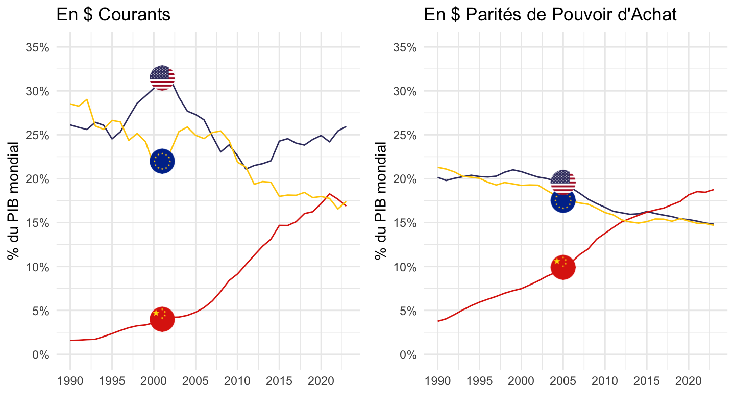
plot1 <- NY.GDP.MKTP.CD |>
  right_join(iso2c, by = "iso2c") |>
  filter(iso2c %in% c("1W", "US", "CN", "XC")) |>
  group_by(year) |>
  filter(n() > 3) |>
  mutate(value = value/value[iso2c == "1W"]) |>
  year_to_date() |>
  filter(!(iso2c == "1W")) |>
  mutate(Iso2c = ifelse(iso2c == "XC", "Europe", Iso2c)) |>
  filter(date >= as.Date("1990-01-01")) |>
  add_flag_color("Iso2c") |>
  ggplot() + theme_minimal() + scale_color_identity() +
  geom_line(aes(x = date, y = value, color = color)) +
  add_flags +
  theme(legend.title = element_blank(),
        legend.position = c(0.85, 0.85)) +
  scale_x_date(breaks = seq(1950, 2100, 5) |> paste0("-01-01") |> as.Date(),
               labels = date_format("%Y")) +
  scale_y_continuous(breaks = 0.01*seq(0, 70, 5),
                     labels = scales::percent_format(accuracy = 1),
                     limits = 0.01*c(0, 35)) +
  xlab("") + ylab("% du PIB mondial") +
  ggtitle("En $ Courants")

plot2 <- NY.GDP.MKTP.PP.CD |>
  right_join(iso2c, by = "iso2c") |>
  filter(iso2c %in% c("1W", "US", "CN", "XC")) |>
  group_by(year) |>
  filter(n() > 3) |>
  mutate(value = value/value[iso2c == "1W"]) |>
  year_to_date() |>
  filter(!(iso2c == "1W")) |>
  mutate(Iso2c = ifelse(iso2c == "XC", "Europe", Iso2c)) |>
  filter(date >= as.Date("1990-01-01")) |>
  add_flag_color("Iso2c") |>
  ggplot() + theme_minimal() + scale_color_identity() +
  geom_line(aes(x = date, y = value, color = color)) +
  add_flags +
  theme(legend.title = element_blank(),
        legend.position = c(0.85, 0.85)) +
  scale_x_date(breaks = seq(1950, 2100, 5) |> paste0("-01-01") |> as.Date(),
               labels = date_format("%Y")) +
  scale_y_continuous(breaks = 0.01*seq(0, 70, 5),
                     labels = scales::percent_format(accuracy = 1),
                     limits = 0.01*c(0, 35)) +
  xlab("") + ylab("% du PIB mondial") +
  ggtitle("En $ Parités de Pouvoir d'Achat")

ggpubr::ggarrange(plot1, plot2)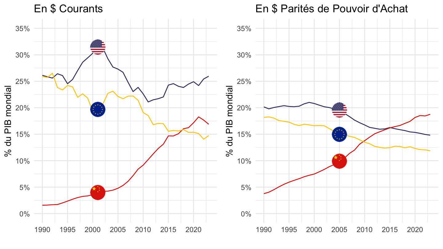
NY.GDP.MKTP.PP.CD |>
  right_join(iso2c, by = "iso2c") |>
  filter(iso2c %in% c("1W", "IT", "FR", "DE", "ES")) |>
  group_by(year) |>
  mutate(value = value/value[iso2c == "1W"]) |>
  year_to_date() |>
  filter(!(iso2c == "1W")) |>
  mutate(Iso2c = ifelse(iso2c == "EU", "Europe", Iso2c)) |>
  add_flag_color("Iso2c") |>
  ggplot() + theme_minimal() + scale_color_identity() +
  geom_line(aes(x = date, y = value, color = color)) +
  add_flags +
  scale_x_date(breaks = seq(1950, 2100, 5) |> paste0("-01-01") |> as.Date(),
               labels = date_format("%Y")) +
  scale_y_continuous(breaks = 0.01*seq(0, 70, .5),
                     labels = scales::percent_format(accuracy = .1)) +
  xlab("") + ylab("% du PIB mondial en Parité de Pouvoir d'Achat")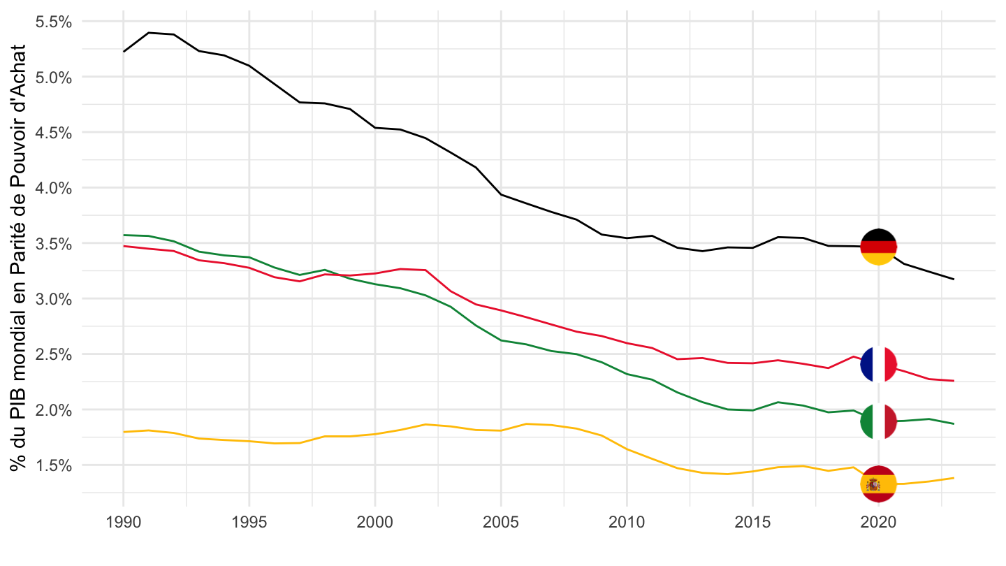
NY.GDP.MKTP.PP.CD |>
  right_join(iso2c, by = "iso2c") |>
  filter(iso2c %in% c("1W", "IT", "FR", "DE", "ES")) |>
  group_by(year) |>
  mutate(value = value/value[iso2c == "1W"]) |>
  year_to_date() |>
  filter(!(iso2c == "1W")) |>
  mutate(Iso2c = ifelse(iso2c == "EU", "Europe", Iso2c)) |>
  add_flag_color("Iso2c") |>
  ggplot() + theme_minimal() + scale_color_identity() +
  geom_line(aes(x = date, y = value, color = color)) +
  add_flags +
  scale_x_date(breaks = seq(1950, 2100, 5) |> paste0("-01-01") |> as.Date(),
               labels = date_format("%Y")) +
  scale_y_log10(breaks = 0.01*seq(0, 70, .5),
                     labels = scales::percent_format(accuracy = .1)) +
  xlab("") + ylab("% du PIB mondial en Parité de Pouvoir d'Achat")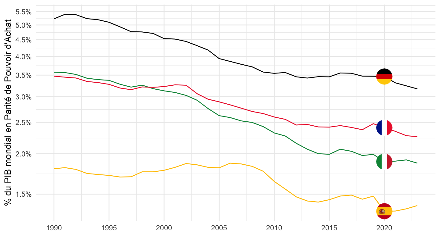
NY.GDP.MKTP.PP.CD |>
  right_join(iso2c, by = "iso2c") |>
  filter(iso2c %in% c("1W", "ID", "KR", "RU")) |>
  group_by(year) |>
  mutate(value = value/value[iso2c == "1W"]) |>
  year_to_date() |>
  filter(!(iso2c == "1W")) |>
  mutate(Iso2c = ifelse(iso2c == "EU", "Europe", Iso2c)) |>
  mutate(Iso2c = ifelse(iso2c == "KR", "Korea", Iso2c)) |>
  mutate(Iso2c = ifelse(iso2c == "RU", "Russia", Iso2c)) |>
  add_flag_color("Iso2c") |>
  ggplot() + theme_minimal() + scale_color_identity() +
  geom_line(aes(x = date, y = value, color = color)) +
  add_flags +
  scale_x_date(breaks = seq(1950, 2100, 5) |> paste0("-01-01") |> as.Date(),
               labels = date_format("%Y")) +
  scale_y_continuous(breaks = 0.01*seq(0, 70, 0.5),
                     labels = scales::percent_format(accuracy = .1)) +
  xlab("") + ylab("% du World GDP")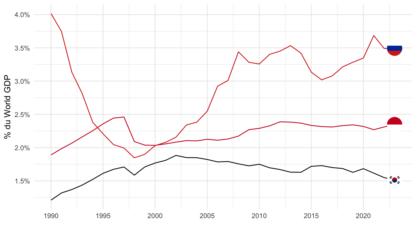
NY.GDP.MKTP.PP.CD |>
  right_join(iso2c, by = "iso2c") |>
  filter(iso2c %in% c("1W", "IN", "JP", "GB")) |>
  group_by(year) |>
  mutate(value = value/value[iso2c == "1W"]) |>
  year_to_date() |>
  filter(!(iso2c == "1W")) |>
  mutate(Iso2c = ifelse(iso2c == "EU", "Europe", Iso2c)) |>
  add_flag_color("Iso2c") |>
  ggplot() + theme_minimal() + scale_color_identity() +
  geom_line(aes(x = date, y = value, color = color)) +
  add_flags +
  scale_x_date(breaks = seq(1950, 2100, 5) |> paste0("-01-01") |> as.Date(),
               labels = date_format("%Y")) +
  scale_y_continuous(breaks = 0.01*seq(0, 70, 2),
                     labels = scales::percent_format(accuracy = 1),
                     limits = 0.01*c(0, 10)) +
  xlab("") + ylab("% of World GDP")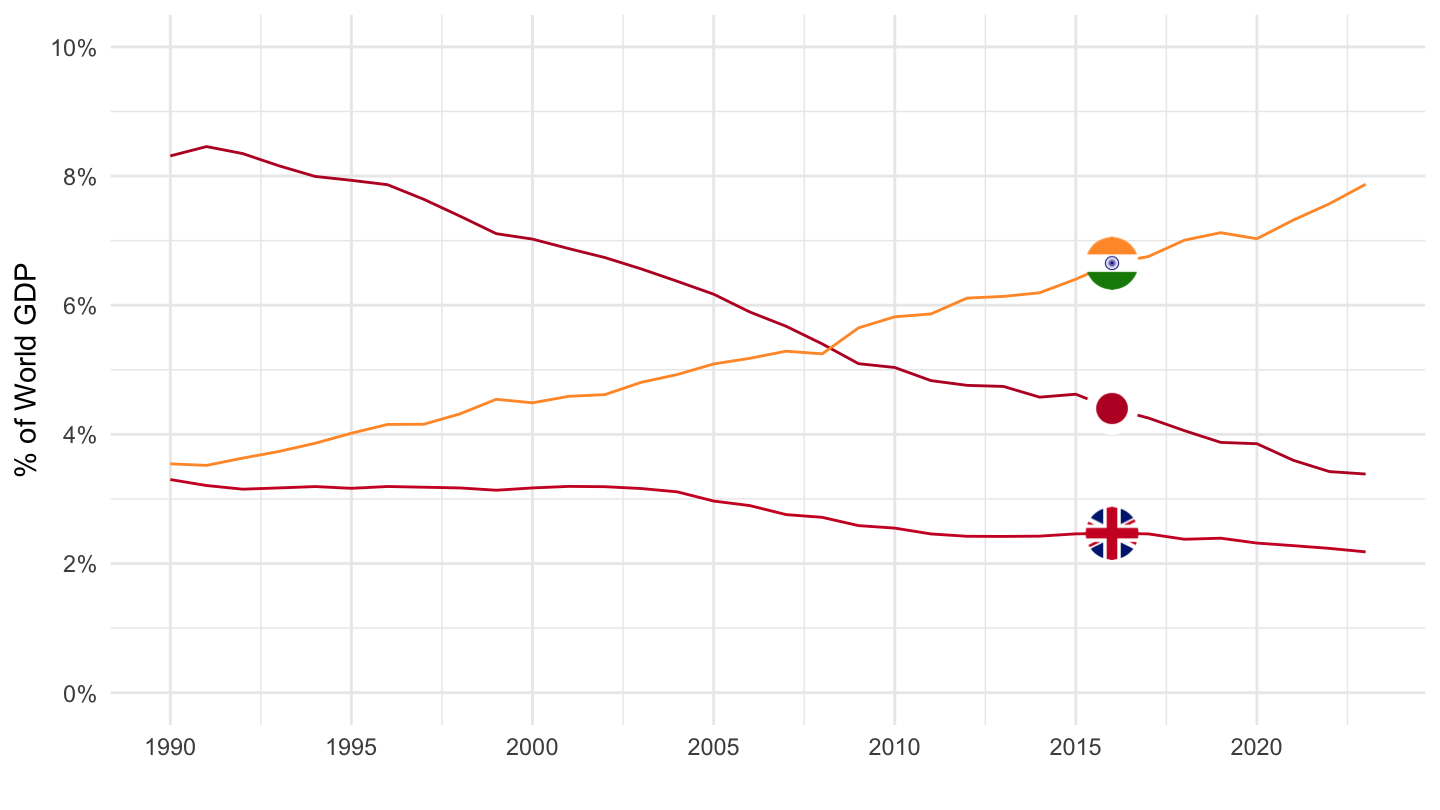
NY.GDP.MKTP.PP.CD |>
  right_join(iso2c, by = "iso2c") |>
  filter(iso2c %in% c("1W", "DE", "FR", "IT")) |>
  group_by(year) |>
  mutate(value = value/value[iso2c == "1W"]) |>
  year_to_date() |>
  filter(!(iso2c == "1W")) |>
  mutate(Iso2c = ifelse(iso2c == "EU", "Europe", Iso2c)) |>
  add_flag_color("Iso2c") |>
  ggplot() + theme_minimal() + scale_color_identity() +
  geom_line(aes(x = date, y = value, color = color)) +
  add_flags +
  scale_x_date(breaks = seq(1950, 2100, 5) |> paste0("-01-01") |> as.Date(),
               labels = date_format("%Y")) +
  scale_y_continuous(breaks = 0.01*seq(0, 70, 2),
                     labels = scales::percent_format(accuracy = 1),
                     limits = 0.01*c(0, 6)) +
  xlab("") + ylab("% of World GDP")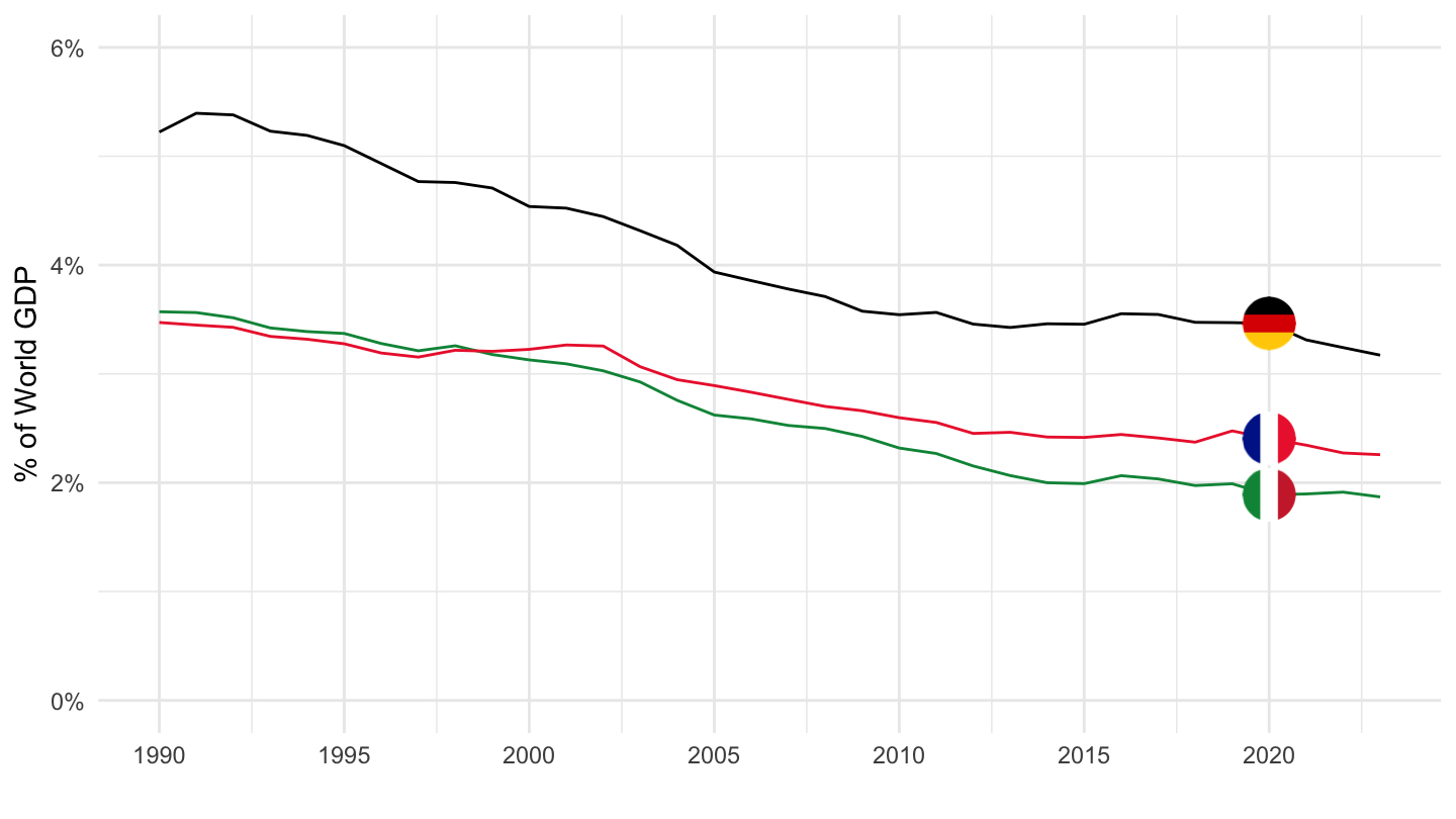
NY.GDP.MKTP.PP.CD |>
  right_join(iso2c, by = "iso2c") |>
  filter(iso2c %in% c("1W", "XC", "US", "EU")) |>
  group_by(year) |>
  mutate(value = value/value[iso2c == "1W"]) |>
  year_to_date() |>
  filter(!(iso2c == "1W")) |>
  mutate(Iso2c = ifelse(iso2c == "EU", "Europe", Iso2c)) |>
  add_flag_color("Iso2c") |>
  ggplot() + theme_minimal() + scale_color_identity() +
  geom_line(aes(x = date, y = value, color = color)) +
  add_flags +
  scale_x_date(breaks = seq(1950, 2100, 5) |> paste0("-01-01") |> as.Date(),
               labels = date_format("%Y")) +
  scale_y_continuous(breaks = 0.01*seq(0, 70, 5),
                     labels = scales::percent_format(accuracy = 1),
                     limits = 0.01*c(0, 25)) +
  xlab("") + ylab("% of World GDP")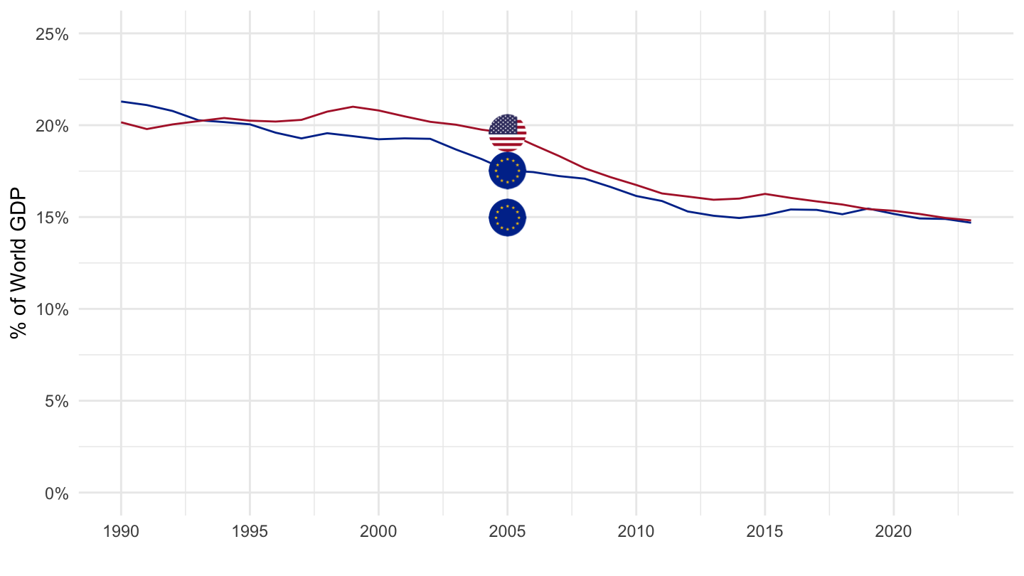
NY.GDP.MKTP.PP.CD |>
  right_join(iso2c, by = "iso2c") |>
  filter(iso2c %in% c("1W", "JP", "DE", "GB")) |>
  group_by(year) |>
  mutate(value = value/value[iso2c == "1W"]) |>
  year_to_date() |>
  filter(!(iso2c == "1W")) |>
  mutate(Iso2c = ifelse(iso2c == "EU", "Europe", Iso2c)) |>
  add_flag_color("Iso2c") |>
  ggplot() + theme_minimal() + scale_color_identity() +
  geom_line(aes(x = date, y = value, color = color)) +
  add_flags +
  scale_x_date(breaks = seq(1950, 2100, 5) |> paste0("-01-01") |> as.Date(),
               labels = date_format("%Y")) +
  scale_y_continuous(breaks = 0.01*seq(0, 70, 2),
                     labels = scales::percent_format(accuracy = 1),
                     limits = 0.01*c(0, 10)) +
  xlab("") + ylab("% of World GDP")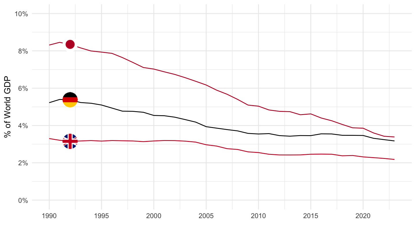
NY.GDP.MKTP.PP.CD |>
  right_join(iso2c, by = "iso2c") |>
  filter(iso2c %in% c("1W", "GB", "FR", "IT")) |>
  group_by(year) |>
  mutate(value = value/value[iso2c == "1W"]) |>
  year_to_date() |>
  filter(!(iso2c == "1W")) |>
  mutate(Iso2c = ifelse(iso2c == "EU", "Europe", Iso2c)) |>
  add_flag_color("Iso2c") |>
  ggplot() + theme_minimal() + scale_color_identity() +
  geom_line(aes(x = date, y = value, color = color)) +
  add_flags +
  scale_x_date(breaks = seq(1950, 2100, 5) |> paste0("-01-01") |> as.Date(),
               labels = date_format("%Y")) +
  scale_y_continuous(breaks = 0.01*seq(0, 70, 0.5),
                     labels = scales::percent_format(accuracy = .1)) +
  xlab("") + ylab("% of World GDP")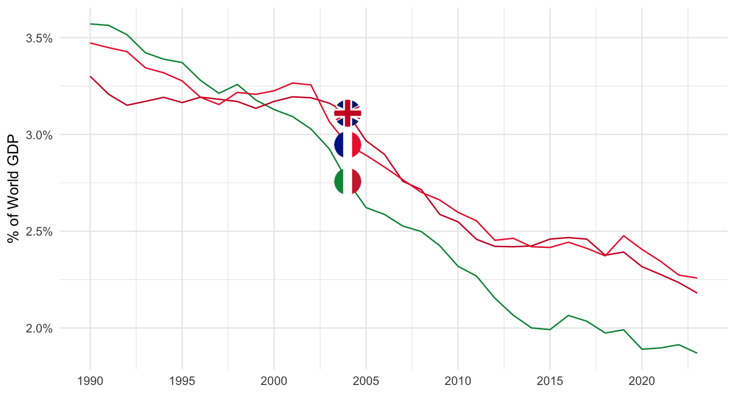
NY.GDP.MKTP.PP.CD |>
  right_join(iso2c, by = "iso2c") |>
  filter(iso2c %in% c("1W", "BR", "RU", "IN")) |>
  mutate(Iso2c = ifelse(iso2c == "RU", "Russia", Iso2c)) |>
  group_by(year) |>
  mutate(value = value/value[iso2c == "1W"]) |>
  year_to_date() |>
  filter(!(iso2c == "1W")) |>
  mutate(Iso2c = ifelse(iso2c == "EU", "Europe", Iso2c)) |>
  add_flag_color("Iso2c") |>
  ggplot() + theme_minimal() + scale_color_identity() +
  geom_line(aes(x = date, y = value, color = color)) +
  add_flags +
  scale_x_date(breaks = seq(1950, 2100, 5) |> paste0("-01-01") |> as.Date(),
               labels = date_format("%Y")) +
  scale_y_continuous(breaks = 0.01*seq(0, 70, 1),
                     labels = scales::percent_format(accuracy = 1)) +
  xlab("") + ylab("% of World GDP")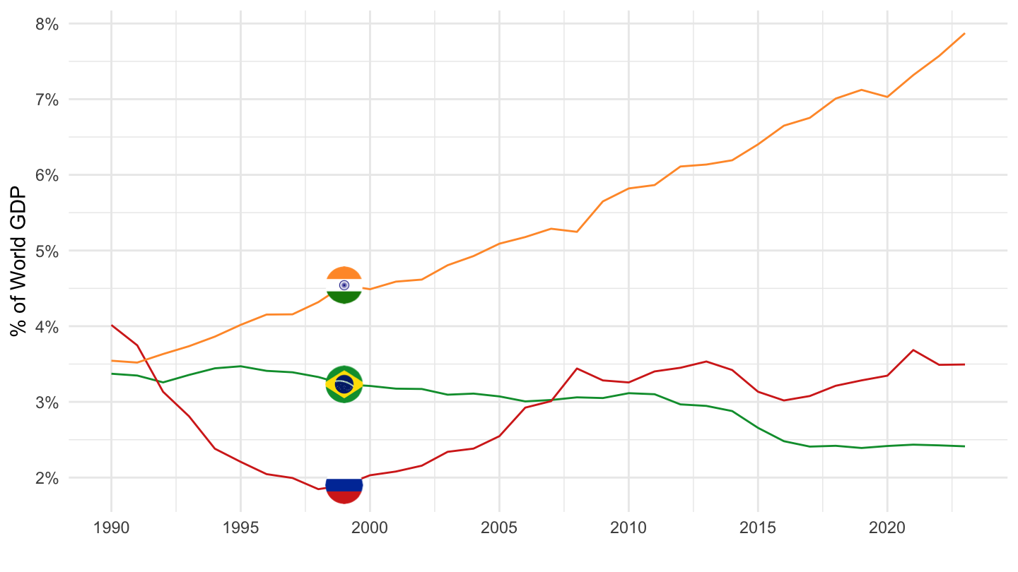
| source | dataset | Title | Updated |
|---|---|---|---|
| source | dataset | Title | Updated |
|---|---|---|---|


