| source | dataset | Title | .html | .rData |
|---|---|---|---|---|
| wdi | NV.IND.TOTL.ZS | Industry, value added (including construction) (% of GDP) | 2025-05-24 | 2026-07-23 |
Industry, value added (including construction) (% of GDP)
Data - WDI
Info
Data on industry
| source | dataset | Title | .html | .rData |
|---|---|---|---|---|
| wdi | NV.IND.TOTL.ZS | Industry, value added (including construction) (% of GDP) | 2025-05-24 | 2026-07-23 |
| ec | INDUSTRY | Industry (sector data) | 2026-07-23 | 2026-07-23 |
| eurostat | ei_isin_m | Industry - monthly data - index (2015 = 100) (NACE Rev. 2) - ei_isin_m | 2026-07-22 | 2026-07-23 |
| eurostat | htec_trd_group4 | High-tech trade by high-tech group of products in million euro (from 2007, SITC Rev. 4) | 2026-07-22 | 2026-07-23 |
| eurostat | nama_10_a64 | National accounts aggregates by industry (up to NACE A*64) | 2026-07-17 | 2026-07-23 |
| eurostat | nama_10_a64_e | National accounts employment data by industry (up to NACE A*64) | 2026-07-24 | 2026-07-23 |
| eurostat | namq_10_a10_e | Employment A*10 industry breakdowns | 2026-07-24 | 2026-07-23 |
| eurostat | road_eqr_carmot | New registrations of passenger cars by type of motor energy and engine size - road_eqr_carmot | 2026-07-24 | 2026-07-23 |
| eurostat | sts_inpp_m | Producer prices in industry, total - monthly data | 2026-07-21 | 2026-07-23 |
| eurostat | sts_inppd_m | Producer prices in industry, domestic market - monthly data | 2026-07-21 | 2026-07-23 |
| eurostat | sts_inpr_m | Production in industry - monthly data | 2026-07-21 | 2026-07-23 |
| eurostat | sts_intvnd_m | Turnover in industry, non domestic market - monthly data - sts_intvnd_m | 2026-07-24 | 2026-07-23 |
| fred | industry | Manufacturing, Industry | 2026-07-23 | 2026-07-23 |
| oecd | ALFS_EMP | Employment by activities and status (ALFS) | 2024-04-16 | 2025-05-24 |
| oecd | BERD_MA_SOF | Business enterprise R&D expenditure by main activity (focussed) and source of funds | 2024-04-16 | 2023-09-09 |
| oecd | GBARD_NABS2007 | Government budget allocations for R and D | 2024-04-16 | 2023-11-22 |
| oecd | MEI_REAL | Production and Sales (MEI) | 2024-05-12 | 2025-05-24 |
| oecd | MSTI_PUB | Main Science and Technology Indicators | 2024-09-15 | 2025-05-24 |
| oecd | SNA_TABLE4 | PPPs and exchange rates | 2024-09-15 | 2025-05-24 |
| wdi | NV.IND.EMPL.KD | Industry, value added per worker (constant 2010 USD) | 2024-01-06 | 2026-07-23 |
| wdi | NV.IND.MANF.CD | Manufacturing, value added (current USD) | 2026-07-23 | 2026-07-23 |
| wdi | NV.IND.MANF.ZS | Manufacturing, value added (% of GDP) | 2025-05-24 | 2026-07-23 |
| wdi | NV.IND.TOTL.KD | Industry (including construction), value added (constant 2015 USD) - NV.IND.TOTL.KD | 2024-01-06 | 2026-07-23 |
| wdi | SL.IND.EMPL.ZS | Employment in industry (% of total employment) | 2026-07-23 | 2026-07-23 |
| wdi | TX.VAL.MRCH.CD.WT | Merchandise exports (current USD) | 2024-01-06 | 2026-07-23 |
LAST_COMPILE
| LAST_COMPILE |
|---|
| 2026-07-24 |
Last
Code
NV.IND.TOTL.ZS %>%
  group_by(year) %>%
  summarise(Nobs = n()) %>%
  arrange(desc(year)) %>%
  head(1) %>%
print_table_conditional()| year | Nobs |
|---|---|
| 2025 | 199 |
Nobs - Javascript
Code
NV.IND.TOTL.ZS %>%
  left_join(iso2c, by = "iso2c") %>%
  group_by(iso2c, Iso2c) %>%
  mutate(value = round(value, 1)) %>%
  summarise(Nobs = n(),
            `Year 1` = first(year),
            `Industry Share 1 (%)` = first(value),
            `Year 2` = last(year),
            `Industry Share 2 (%)` = last(value)) %>%
  arrange(-Nobs) %>%
  mutate(Flag = gsub(" ", "-", str_to_lower(Iso2c)),
         Flag = paste0('<img src="../../bib/flags/vsmall/', Flag, '.png" alt="Flag">')) %>%
  select(Flag, everything()) %>%
  {if (is_html_output()) datatable(., filter = 'top', rownames = F, escape = F) else .}
Crises in Emerging Markets (Source: Vegh (2013))
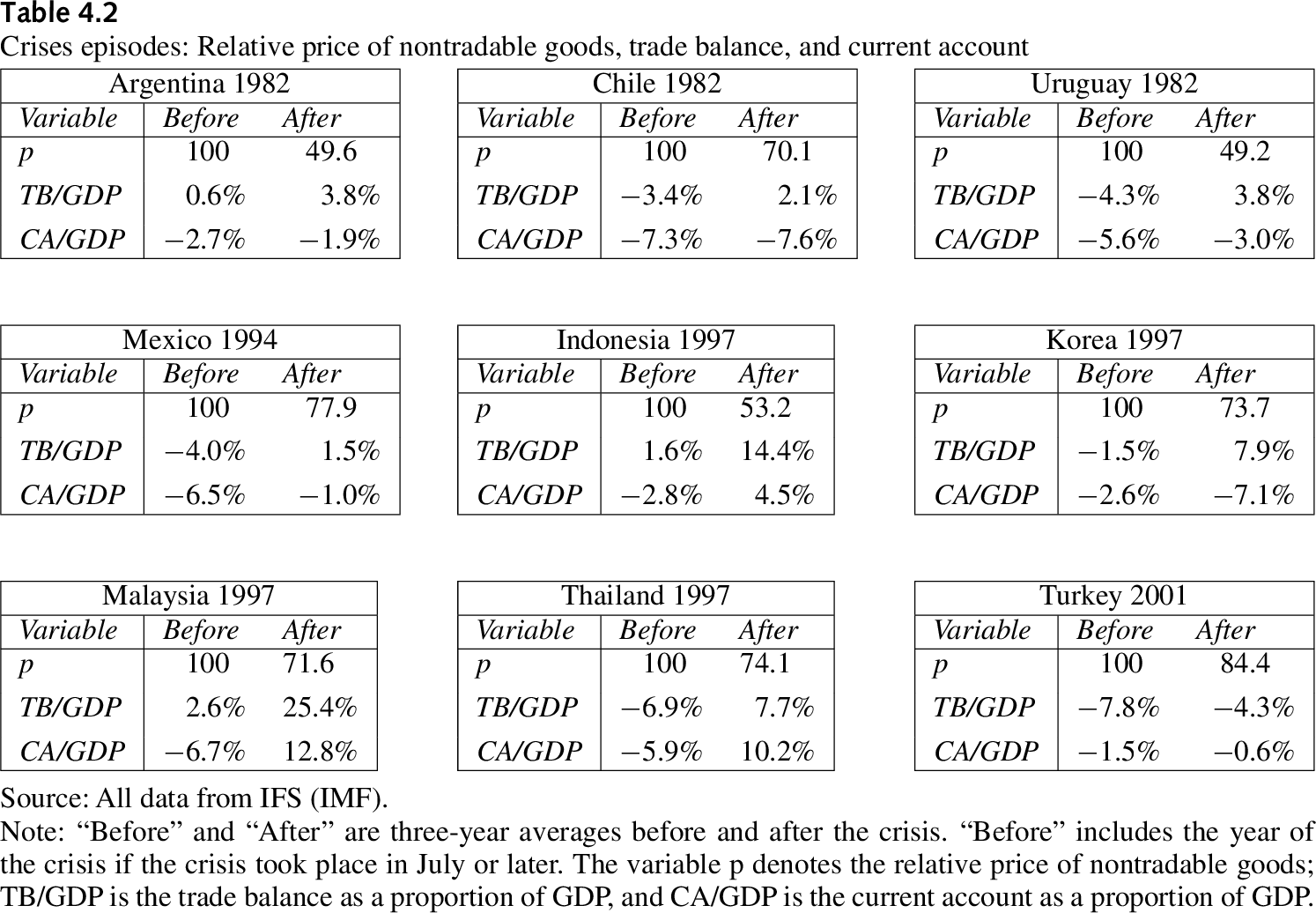
1982: Southern Cone - Argentina, Chile, Uruguay
Code
NV.IND.TOTL.ZS %>%
  year_to_date %>%
  filter(iso2c %in% c("AR", "CL", "UY"),
         date >= as.Date("1976-01-01"),
            date <= as.Date("1986-01-01")) %>%
  left_join(iso2c, by = "iso2c") %>%
  left_join(colors, by = c("Iso2c" = "country")) %>%
  mutate(value = value/100) %>%
  ggplot(.) + geom_line(aes(x = date, y = value, color = color)) +
  xlab("") + ylab("Industry, value added (% of GDP)") +
  theme_minimal() + scale_color_identity() + add_3flags +
  scale_x_date(breaks = seq(1950, 2100, 1) %>% paste0("-01-01") %>% as.Date,
               labels = date_format("%Y")) +
  scale_y_continuous(breaks = 0.01*seq(-60, 60, 2),
                     labels = scales::percent_format(accuracy = 1))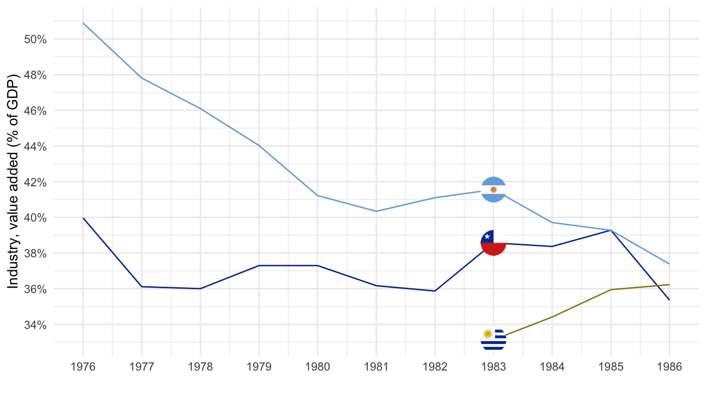
1994: Mexico
Code
NV.IND.TOTL.ZS %>%
  year_to_date %>%
  filter(iso2c %in% c("MX"),
         date <= as.Date("1999-01-01"),
         date >= as.Date("1989-01-01")) %>%
  left_join(iso2c, by = "iso2c") %>%
  ggplot(.) +
  geom_line(aes(x = date, y = value/100)) +
  theme_minimal() + scale_color_manual(values = viridis(5)[1:4]) +
  theme(legend.title = element_blank(),
        legend.position = c(0.2, 0.8)) +
  scale_x_date(breaks = seq(1950, 2100, 1) %>% paste0("-01-01") %>% as.Date,
               labels = date_format("%Y")) +
  scale_y_continuous(breaks = 0.01*seq(-60, 60, 1),
                     labels = scales::percent_format(accuracy = 1)) +
  xlab("") + ylab("Industry, value added (% of GDP)")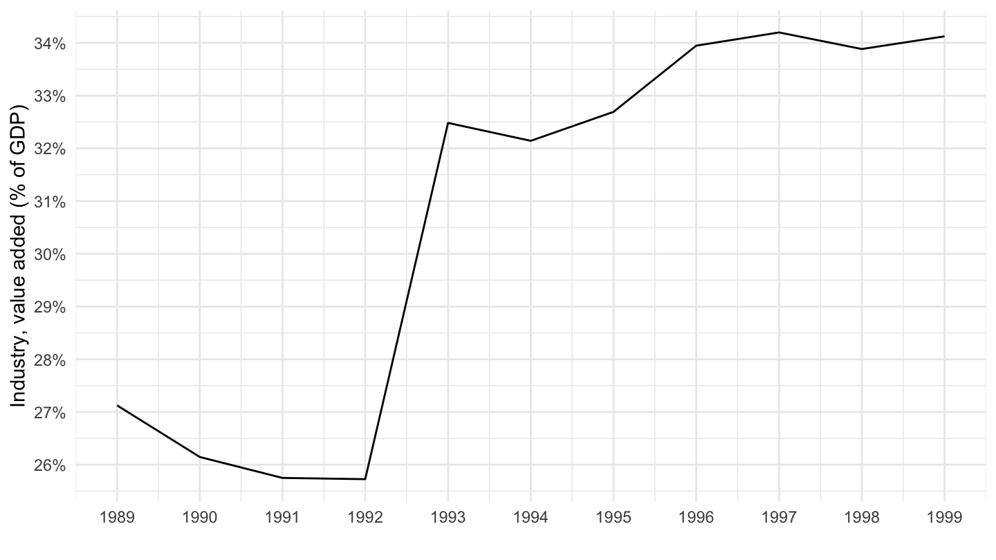
1997: East Asia - Indonesia, Korea, Malaysia, Thailand
Code
NV.IND.TOTL.ZS %>%
  year_to_date %>%
  filter(iso2c %in% c("ID", "KR", "MY", "TH"),
         date <= as.Date("2002-01-01"),
         date >= as.Date("1992-01-01")) %>%
  left_join(iso2c, by = "iso2c") %>%
  mutate(Iso2c = ifelse(iso2c == "KR", "South Korea", Iso2c)) %>%
  left_join(colors, by = c("Iso2c" = "country")) %>%
  mutate(value = value/100) %>%
  ggplot(.) + geom_line(aes(x = date, y = value, color = color)) +
  xlab("") + ylab("Industry, value added (% of GDP)") +
  theme_minimal() + scale_color_identity() + add_4flags +
  scale_x_date(breaks = seq(1950, 2100, 1) %>% paste0("-01-01") %>% as.Date,
               labels = date_format("%Y")) +
  scale_y_continuous(breaks = 0.01*seq(-60, 60, 2),
                     labels = scales::percent_format(accuracy = 1))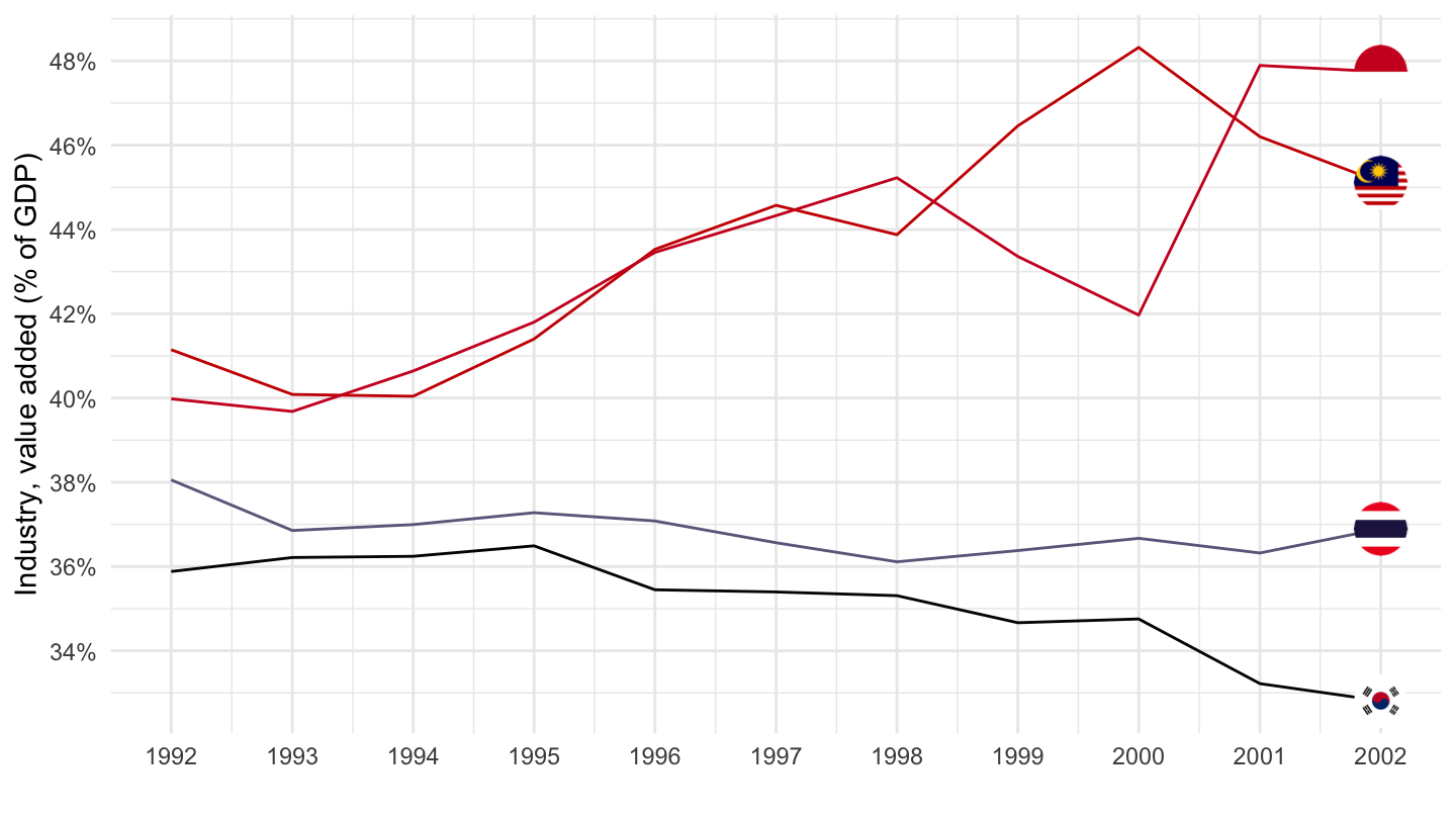
2001: Turkey
Code
NV.IND.TOTL.ZS %>%
  year_to_date %>%
  filter(iso2c %in% c("TR"),
         date <= as.Date("2006-01-01"),
         date >= as.Date("1996-01-01")) %>%
  left_join(iso2c, by = "iso2c") %>%
  ggplot(.) +
  geom_line(aes(x = date, y = value/100)) +
  theme_minimal() + scale_color_manual(values = viridis(5)[1:4]) +
  theme(legend.title = element_blank(),
        legend.position = c(0.2, 0.8)) +
  scale_x_date(breaks = seq(1950, 2100, 1) %>% paste0("-01-01") %>% as.Date,
               labels = date_format("%Y")) +
  scale_y_continuous(breaks = 0.01*seq(-60, 60, 1),
                     labels = scales::percent_format(accuracy = 1)) +
  xlab("") + ylab("Industry, value added (% of GDP)")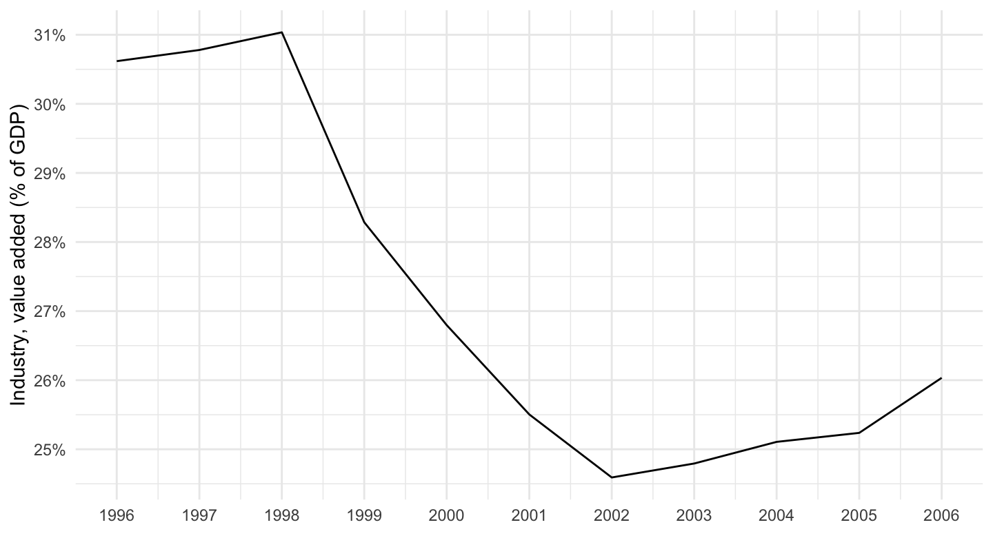
2002: Uruguay
Code
NV.IND.TOTL.ZS %>%
  year_to_date %>%
  filter(iso2c %in% c("UY"),
         date <= as.Date("2008-01-01"),
         date >= as.Date("1996-01-01")) %>%
  left_join(iso2c, by = "iso2c") %>%
  ggplot(.) +
  geom_line(aes(x = date, y = value/100)) +
  theme_minimal() + scale_color_manual(values = viridis(5)[1:4]) +
  theme(legend.title = element_blank(),
        legend.position = c(0.2, 0.8)) +
  scale_x_date(breaks = seq(1950, 2100, 1) %>% paste0("-01-01") %>% as.Date,
               labels = date_format("%Y")) +
  scale_y_continuous(breaks = 0.01*seq(-60, 60, 1),
                     labels = scales::percent_format(accuracy = 1)) +
  xlab("") + ylab("Industry, value added (% of GDP)")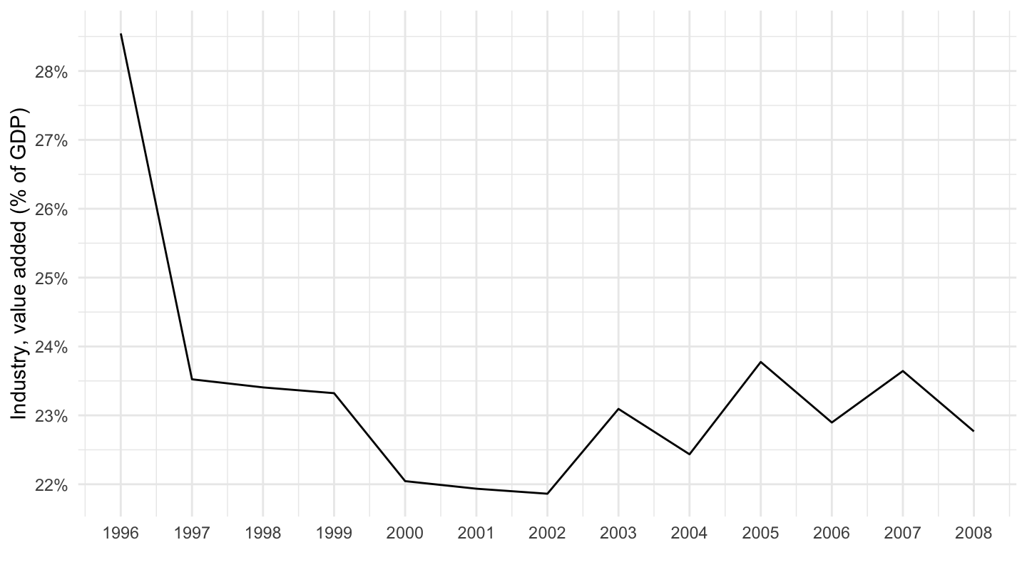
Iceland
Code
NV.IND.TOTL.ZS %>%
  filter(iso2c %in% c("IS")) %>%
  left_join(iso2c, by = "iso2c") %>%
  year_to_date %>%
  ggplot(.) + geom_line(aes(x = date, y = value/100)) +
  xlab("") + ylab("Industry, value added (% of GDP)") + theme_minimal() +
  theme(legend.title = element_blank(),
        legend.position = c(0.2, 0.2)) +
  scale_x_date(breaks = seq(1950, 2100, 2) %>% paste0("-01-01") %>% as.Date,
               labels = date_format("%Y")) +
  scale_y_continuous(breaks = 0.01*seq(-60, 60, 1),
                     labels = scales::percent_format(accuracy = 1))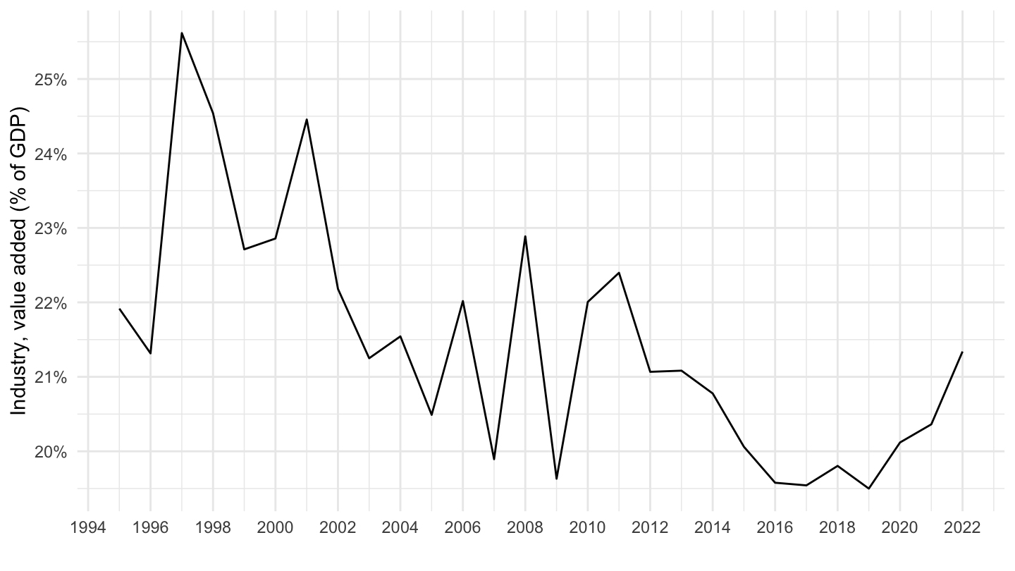
Japan
Code
NV.IND.TOTL.ZS %>%
  filter(iso2c %in% c("JP")) %>%
  left_join(iso2c, by = "iso2c") %>%
  year_to_date %>%
  ggplot(.) + geom_line(aes(x = date, y = value/100)) +
  xlab("") + ylab("Industry, value added (% of GDP)") + theme_minimal() +
  theme(legend.title = element_blank(),
        legend.position = c(0.2, 0.2)) +
  scale_x_date(breaks = seq(1950, 2100, 2) %>% paste0("-01-01") %>% as.Date,
               labels = date_format("%Y")) +
  scale_y_continuous(breaks = 0.01*seq(-60, 60, 1),
                     labels = scales::percent_format(accuracy = 1))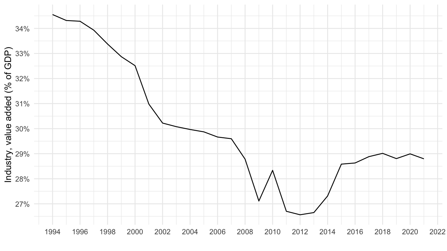
World, France, Germany
All
Code
NV.IND.TOTL.ZS %>%
  filter(iso2c %in% c("DE", "1W", "FR")) %>%
  left_join(iso2c, by = "iso2c") %>%
  year_to_date %>%
  mutate(value = value/100) %>%
  ggplot(.) + xlab("") + ylab("Industry, value added (% of GDP)") +
  geom_line(aes(x = date, y = value, color = Iso2c)) + add_3flags +
  theme_minimal() + scale_color_manual(values = c("#002395", "#DD0000", "#000000")) +
  theme(legend.title = element_blank(),
        legend.position = c(0.2, 0.2)) +
  scale_x_date(breaks = seq(1950, 2100, 5) %>% paste0("-01-01") %>% as.Date,
               labels = date_format("%Y")) +
  scale_y_log10(breaks = 0.01*seq(-60, 60, 2),
                     labels = scales::percent_format(accuracy = 1))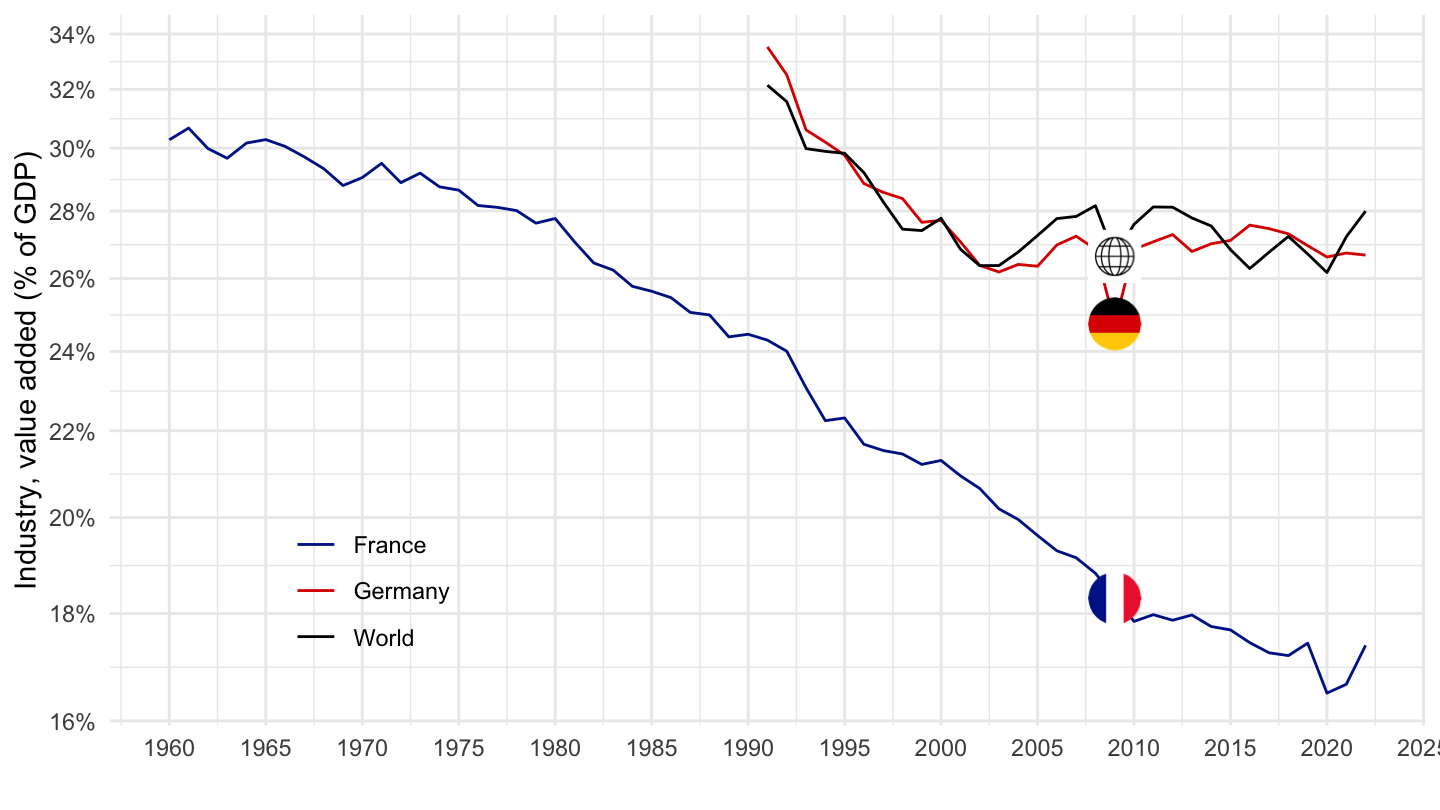
1990-
Code
NV.IND.TOTL.ZS %>%
  filter(iso2c %in% c("DE", "1W", "FR")) %>%
  left_join(iso2c, by = "iso2c") %>%
  year_to_date %>%
  filter(date >= as.Date("1990-01-01")) %>%
  mutate(value = value/100) %>%
  ggplot(.) + xlab("") + ylab("Industry, value added (% of GDP)") +
  geom_line(aes(x = date, y = value, color = Iso2c)) + add_3flags +
  theme_minimal() + scale_color_manual(values = c("#002395", "#DD0000", "#000000")) +
  theme(legend.title = element_blank(),
        legend.position = c(0.2, 0.2)) +
  scale_x_date(breaks = seq(1950, 2100, 2) %>% paste0("-01-01") %>% as.Date,
               labels = date_format("%Y")) +
  scale_y_log10(breaks = 0.01*seq(-60, 60, 2),
                     labels = scales::percent_format(accuracy = 1))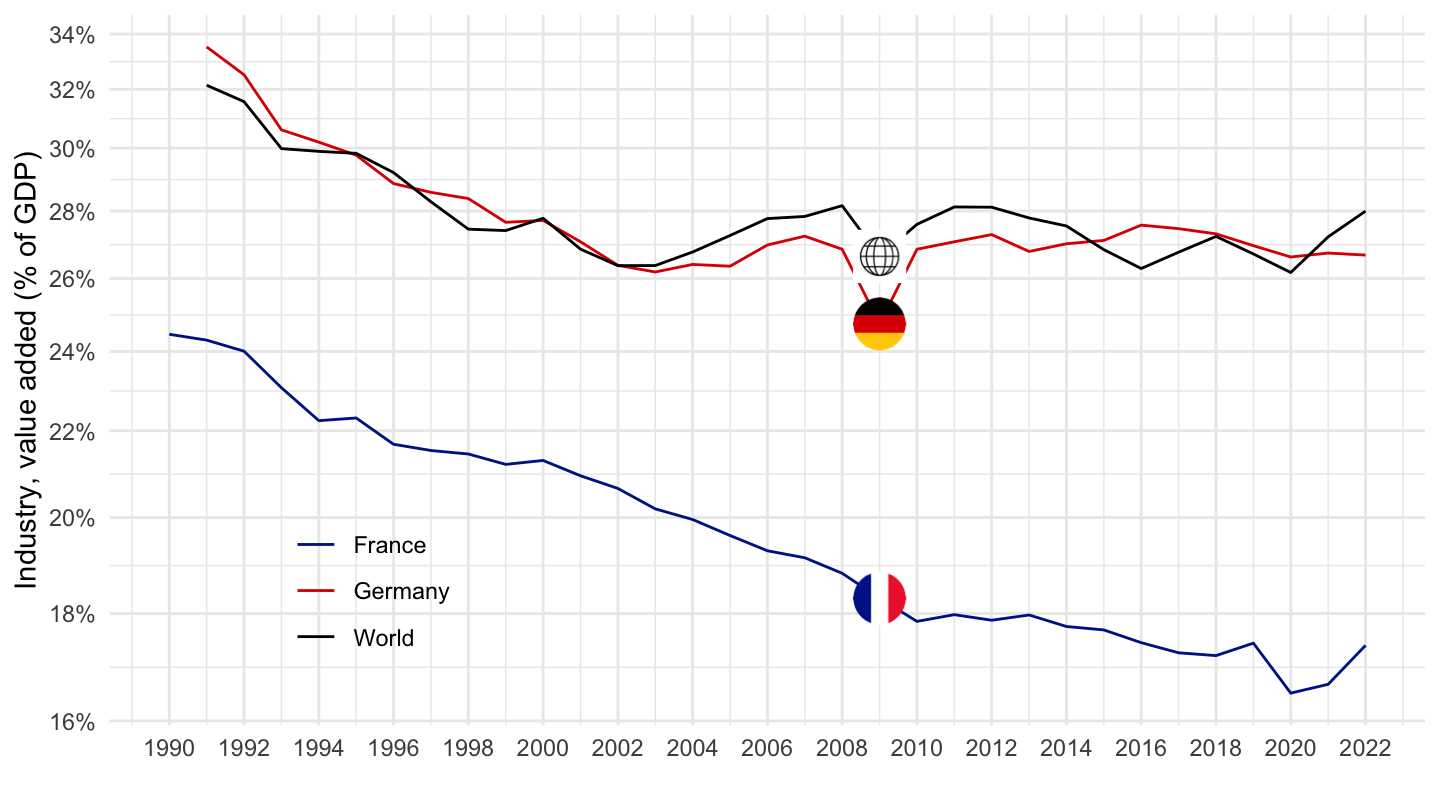
OECD, World, Advanced
Code
NV.IND.TOTL.ZS %>%
  filter(iso2c %in% c("OE", "1W", "EU")) %>%
  left_join(iso2c, by = "iso2c") %>%
  year_to_date %>%
  mutate(Iso2c = ifelse(iso2c == "OE", "OECD Members", Iso2c)) %>%
  left_join(colors, by = c("Iso2c" = "country")) %>%
  mutate(value = value/100) %>%
  ggplot(.) + geom_line(aes(x = date, y = value, color = color)) +
  xlab("") + ylab("Industry, value added (% of GDP)") +
  theme_minimal() + scale_color_identity() + add_3flags +
  scale_x_date(breaks = seq(1950, 2100, 5) %>% paste0("-01-01") %>% as.Date,
               labels = date_format("%Y")) +
  scale_y_continuous(breaks = 0.01*seq(-60, 60, 2),
                     labels = scales::percent_format(accuracy = 1))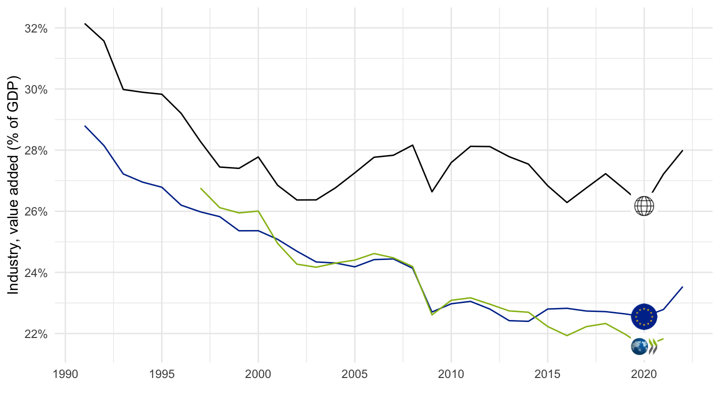
France, Germany, OECD
Code
NV.IND.TOTL.ZS %>%
  filter(iso2c %in% c("OE", "FR", "DE")) %>%
  left_join(iso2c, by = "iso2c") %>%
  year_to_date %>%
  mutate(Iso2c = ifelse(iso2c == "OE", "OECD Members", Iso2c)) %>%
  left_join(colors, by = c("Iso2c" = "country")) %>%
  mutate(value = value/100) %>%
  ggplot(.) + geom_line(aes(x = date, y = value, color = color)) +
  xlab("") + ylab("Industry, value added (% of GDP)") +
  theme_minimal() + scale_color_identity() + add_3flags +
  scale_x_date(breaks = seq(1950, 2100, 5) %>% paste0("-01-01") %>% as.Date,
               labels = date_format("%Y")) +
  scale_y_continuous(breaks = 0.01*seq(-60, 60, 2),
                     labels = scales::percent_format(accuracy = 1))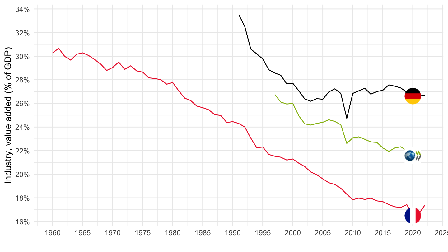
China, France, Germany
Code
NV.IND.TOTL.ZS %>%
  filter(iso2c %in% c("CN", "FR", "DE")) %>%
  left_join(iso2c, by = "iso2c") %>%
  year_to_date %>%
  left_join(colors, by = c("Iso2c" = "country")) %>%
  mutate(value = value/100) %>%
  ggplot(.) + geom_line(aes(x = date, y = value, color = color)) +
  xlab("") + ylab("Industry, value added (% of GDP)") +
  theme_minimal() + scale_color_identity() + add_3flags +
  scale_x_date(breaks = seq(1950, 2100, 5) %>% paste0("-01-01") %>% as.Date,
               labels = date_format("%Y")) +
  scale_y_continuous(breaks = 0.01*seq(-60, 60, 2),
                     labels = scales::percent_format(accuracy = 1))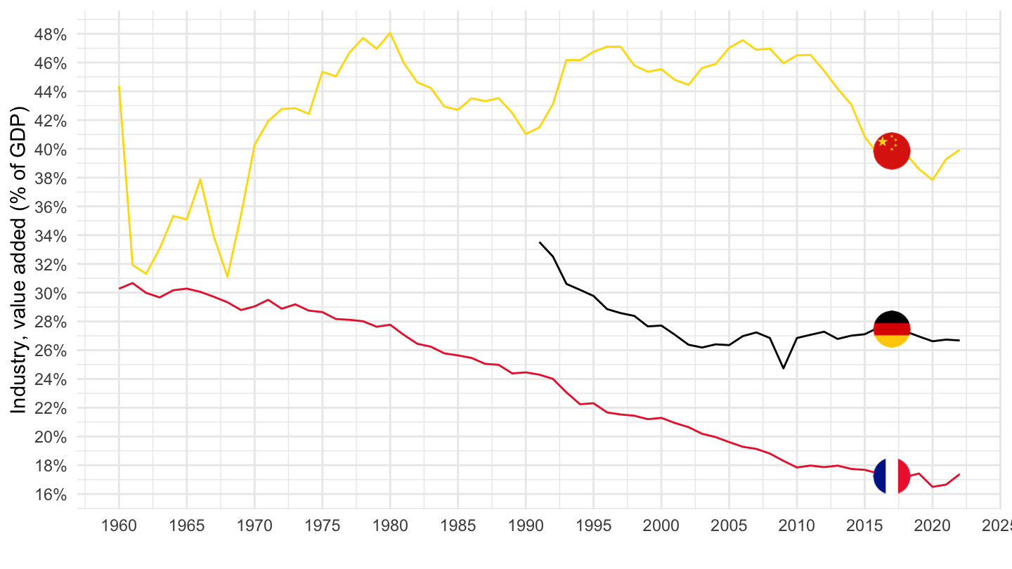
Japan, Iceland, South Korea
Code
NV.IND.TOTL.ZS %>%
  filter(iso2c %in% c("JP", "IS", "KR")) %>%
  left_join(iso2c, by = "iso2c") %>%
  mutate(Iso2c = ifelse(iso2c == "KR", "South Korea", Iso2c)) %>%
  year_to_date %>%
  left_join(colors, by = c("Iso2c" = "country")) %>%
  mutate(value = value/100) %>%
  ggplot(.) + geom_line(aes(x = date, y = value, color = color)) +
  xlab("") + ylab("Industry, value added (% of GDP)") +
  theme_minimal() + scale_color_identity() + add_3flags +
  scale_x_date(breaks = seq(1950, 2100, 5) %>% paste0("-01-01") %>% as.Date,
               labels = date_format("%Y")) +
  scale_y_continuous(breaks = 0.01*seq(-60, 60, 2),
                     labels = scales::percent_format(accuracy = 1))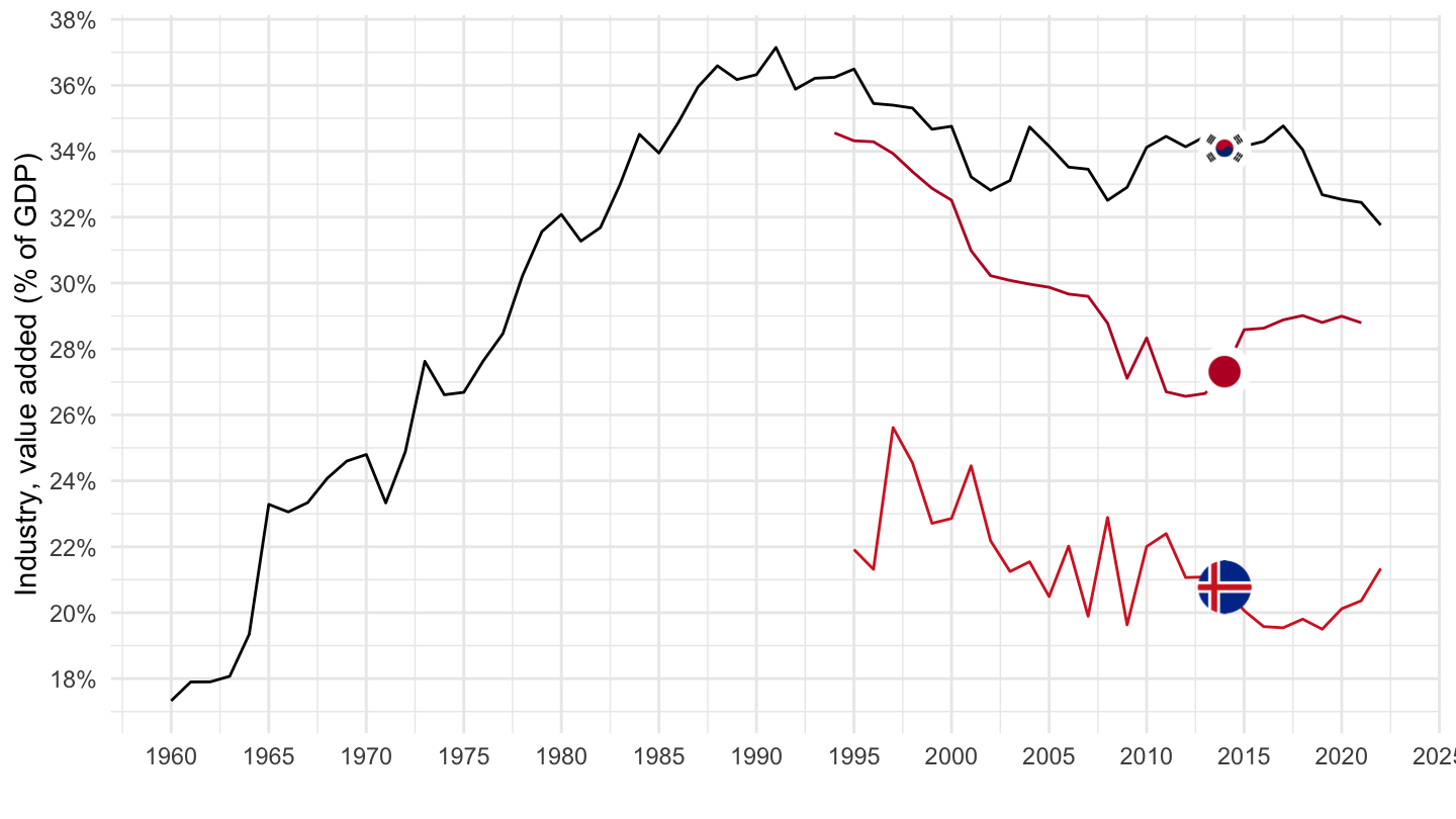
Italy, Portugal, Spain
Code
NV.IND.TOTL.ZS %>%
  filter(iso2c %in% c("ES", "IT", "PT")) %>%
  left_join(iso2c, by = "iso2c") %>%
  year_to_date %>%
  left_join(colors, by = c("Iso2c" = "country")) %>%
  mutate(value = value/100) %>%
  ggplot(.) + geom_line(aes(x = date, y = value, color = color)) +
  xlab("") + ylab("Industry, value added (% of GDP)") +
  theme_minimal() + scale_color_identity() + add_3flags +
  scale_x_date(breaks = seq(1950, 2100, 5) %>% paste0("-01-01") %>% as.Date,
               labels = date_format("%Y")) +
  scale_y_continuous(breaks = 0.01*seq(-60, 60, 2),
                     labels = scales::percent_format(accuracy = 1))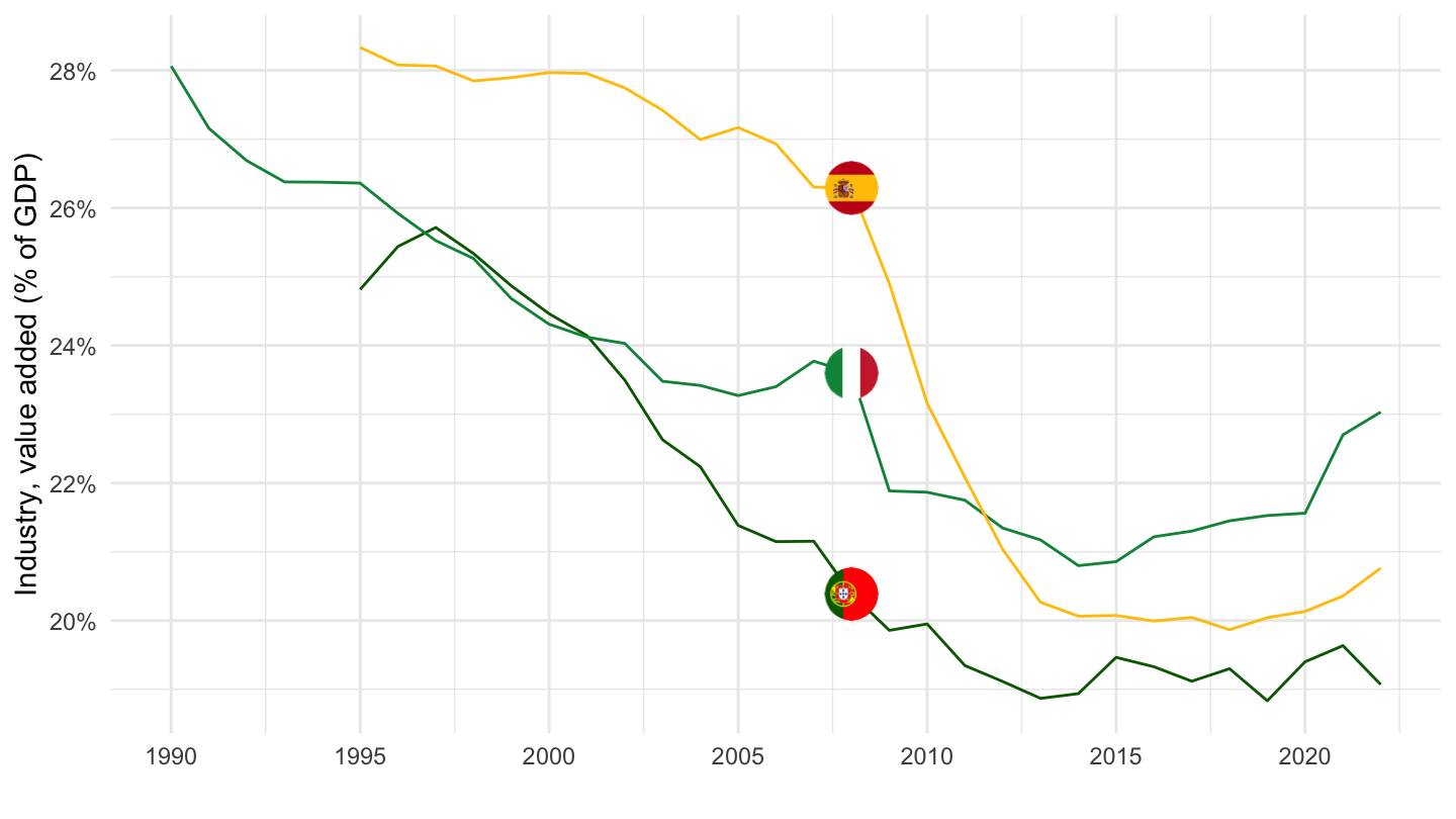
Spain, United Kingdom, United States
Code
NV.IND.TOTL.ZS %>%
  filter(iso2c %in% c("US", "GB", "ES")) %>%
  left_join(iso2c, by = "iso2c") %>%
  year_to_date %>%
  left_join(colors, by = c("Iso2c" = "country")) %>%
  mutate(value = value/100) %>%
  ggplot(.) + geom_line(aes(x = date, y = value, color = color)) +
  xlab("") + ylab("Industry, value added (% of GDP)") +
  theme_minimal() + scale_color_identity() + add_3flags +
  scale_x_date(breaks = seq(1950, 2100, 5) %>% paste0("-01-01") %>% as.Date,
               labels = date_format("%Y")) +
  scale_y_continuous(breaks = 0.01*seq(-60, 60, 2),
                     labels = scales::percent_format(accuracy = 1))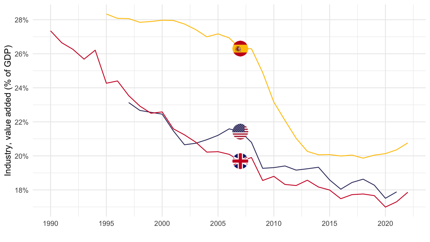
Argentina, Chile, Venezuela
Code
NV.IND.TOTL.ZS %>%
  filter(iso2c %in% c("AR", "CL", "VE")) %>%
  left_join(iso2c, by = "iso2c") %>%
  year_to_date %>%
  mutate(Iso2c = ifelse(iso2c == "VE", "Venezuela", Iso2c)) %>%
  left_join(colors, by = c("Iso2c" = "country")) %>%
  mutate(value = value/100) %>%
  ggplot(.) + geom_line(aes(x = date, y = value, color = color)) +
  xlab("") + ylab("Industry, value added (% of GDP)") +
  theme_minimal() + scale_color_identity() + add_3flags +
  scale_x_date(breaks = seq(1950, 2100, 5) %>% paste0("-01-01") %>% as.Date,
               labels = date_format("%Y")) +
  scale_y_continuous(breaks = 0.01*seq(-60, 60, 2),
                     labels = scales::percent_format(accuracy = 1))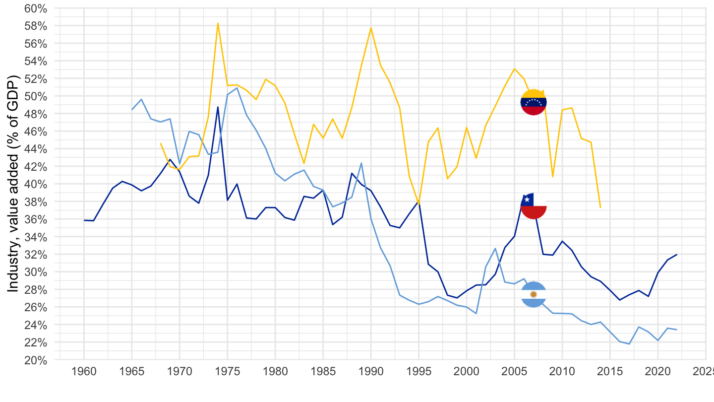
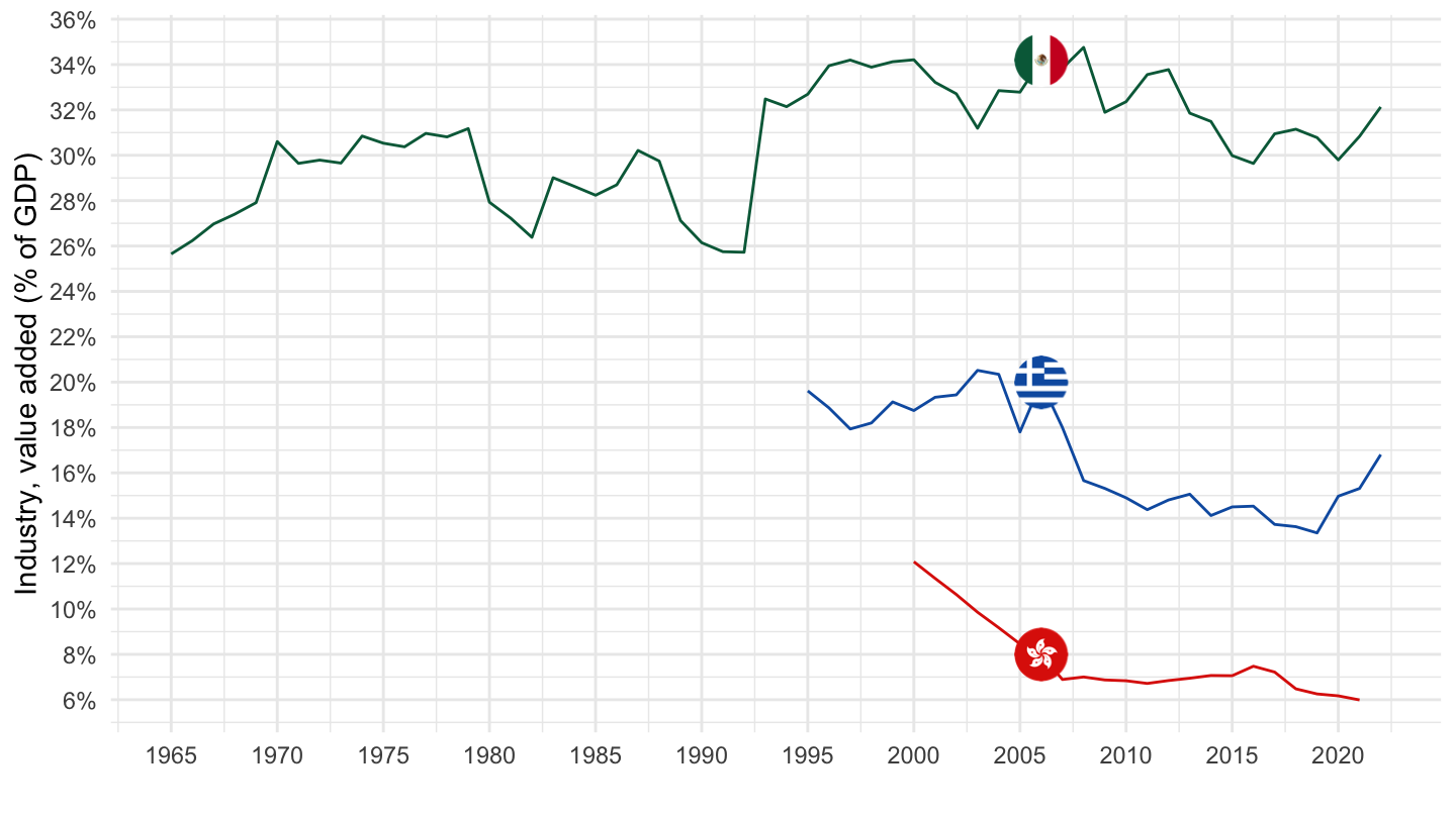
Greece, Hong Kong, Mexico
Code
NV.IND.TOTL.ZS %>%
  filter(iso2c %in% c("GR", "HK", "MX")) %>%
  left_join(iso2c, by = "iso2c") %>%
  mutate(Iso2c = ifelse(iso2c == "HK", "Hong Kong", Iso2c)) %>%
  year_to_date %>%
  left_join(colors, by = c("Iso2c" = "country")) %>%
  mutate(value = value/100) %>%
  ggplot(.) + geom_line(aes(x = date, y = value, color = color)) +
  xlab("") + ylab("Industry, value added (% of GDP)") +
  theme_minimal() + scale_color_identity() + add_3flags +
  scale_x_date(breaks = seq(1950, 2100, 5) %>% paste0("-01-01") %>% as.Date,
               labels = date_format("%Y")) +
  scale_y_continuous(breaks = 0.01*seq(-60, 60, 2),
                     labels = scales::percent_format(accuracy = 1))