| source | dataset | .html | .RData |
|---|---|---|---|
| eurostat | namq_10_a10_e | 2025-05-24 | 2025-05-24 |
Employment A*10 industry breakdowns
Data - Eurostat
Info
Data on employment
| source | dataset | .html | .RData |
|---|---|---|---|
| bls | jt | 2024-11-12 | NA |
| bls | la | 2024-11-12 | NA |
| bls | ln | 2024-11-12 | NA |
| eurostat | nama_10_a10_e | 2025-05-18 | 2025-05-18 |
| eurostat | nama_10_a64_e | 2025-05-24 | 2025-05-24 |
| eurostat | namq_10_a10_e | 2025-05-24 | 2025-05-24 |
| eurostat | une_rt_m | 2025-05-18 | 2025-05-18 |
| oecd | ALFS_EMP | 2024-04-16 | 2025-03-04 |
| oecd | EPL_T | 2024-11-12 | 2023-12-10 |
| oecd | LFS_SEXAGE_I_R | 2024-09-15 | 2024-04-15 |
| oecd | STLABOUR | 2025-01-17 | 2025-01-17 |
Data on industry
| source | dataset | .html | .RData |
|---|---|---|---|
| ec | INDUSTRY | 2025-01-05 | 2023-10-01 |
| eurostat | ei_isin_m | 2025-05-18 | 2025-05-18 |
| eurostat | htec_trd_group4 | 2025-05-18 | 2025-05-18 |
| eurostat | nama_10_a64 | 2025-05-18 | 2025-05-18 |
| eurostat | nama_10_a64_e | 2025-05-24 | 2025-05-24 |
| eurostat | namq_10_a10_e | 2025-05-24 | 2025-05-24 |
| eurostat | road_eqr_carmot | 2025-05-18 | 2025-05-18 |
| eurostat | sts_inpp_m | 2024-06-24 | 2025-05-18 |
| eurostat | sts_inppd_m | 2025-05-18 | 2025-05-18 |
| eurostat | sts_inpr_m | 2025-05-18 | 2025-05-18 |
| eurostat | sts_intvnd_m | 2025-05-24 | 2025-05-24 |
| fred | industry | 2025-05-18 | 2025-05-18 |
| oecd | ALFS_EMP | 2024-04-16 | 2025-03-04 |
| oecd | BERD_MA_SOF | 2024-04-16 | 2023-09-09 |
| oecd | GBARD_NABS2007 | 2024-04-16 | 2023-11-22 |
| oecd | MEI_REAL | 2024-05-12 | 2025-01-31 |
| oecd | MSTI_PUB | 2024-09-15 | 2025-01-31 |
| oecd | SNA_TABLE4 | 2024-09-15 | 2025-03-09 |
| wdi | NV.IND.EMPL.KD | 2024-01-06 | 2025-03-09 |
| wdi | NV.IND.MANF.CD | 2025-03-09 | 2025-03-09 |
| wdi | NV.IND.MANF.ZS | 2025-01-31 | 2025-03-09 |
| wdi | NV.IND.TOTL.KD | 2024-01-06 | 2025-03-09 |
| wdi | NV.IND.TOTL.ZS | 2025-01-31 | 2025-03-09 |
| wdi | SL.IND.EMPL.ZS | 2025-01-31 | 2025-03-09 |
| wdi | TX.VAL.MRCH.CD.WT | 2024-01-06 | 2025-03-09 |
Last
Code
namq_10_a10_e %>%
  group_by(time) %>%
  summarise(Nobs = n()) %>%
  arrange(desc(time)) %>%
  head(2) %>%
print_table_conditional()| time | Nobs |
|---|---|
| 2025Q1 | 4998 |
| 2024Q4 | 25715 |
na_item
Code
namq_10_a10_e %>%
  left_join(na_item, by = "na_item") %>%
  group_by(na_item, Na_item) %>%
  summarise(Nobs = n()) %>%
  arrange(-Nobs) %>%
{if (is_html_output()) print_table(.) else .}| na_item | Na_item | Nobs |
|---|---|---|
| EMP_DC | Total employment domestic concept | 1143753 |
| SAL_DC | Employees domestic concept | 1108824 |
| SELF_DC | Self-employed domestic concept | 1099226 |
unit
namq_10_a10_e
Code
namq_10_a10_e %>%
  left_join(unit, by = "unit") %>%
  group_by(unit, Unit) %>%
  summarise(Nobs = n()) %>%
  arrange(-Nobs) %>%
  {if (is_html_output()) datatable(., filter = 'top', rownames = F) else .}
unit
Code
namq_10_a10_e %>%
  left_join(unit, by = "unit") %>%
  group_by(unit, Unit) %>%
  summarise(Nobs = n()) %>%
  arrange(-Nobs) %>%
  {if (is_html_output()) datatable(., filter = 'top', rownames = F) else .}
nace_r2
Code
namq_10_a10_e %>%
  left_join(nace_r2, by = "nace_r2") %>%
  group_by(nace_r2, Nace_r2) %>%
  summarise(Nobs = n()) %>%
  arrange(-Nobs) %>%
{if (is_html_output()) print_table(.) else .}| nace_r2 | Nace_r2 | Nobs |
|---|---|---|
| TOTAL | Total - all NACE activities | 283625 |
| A | Agriculture, forestry and fishing | 279445 |
| G-I | Wholesale and retail trade, transport, accommodation and food service activities | 279445 |
| B-E | Industry (except construction) | 279369 |
| C | Manufacturing | 279369 |
| F | Construction | 279369 |
| M_N | Professional, scientific and technical activities; administrative and support service activities | 279369 |
| R-U | Arts, entertainment and recreation; other service activities; activities of household and extra-territorial organizations and bodies | 279351 |
| J | Information and communication | 278987 |
| O-Q | Public administration, defence, education, human health and social work activities | 278973 |
| L | Real estate activities | 278595 |
| K | Financial and insurance activities | 275906 |
s_adj
Code
namq_10_a10_e %>%
  left_join(s_adj, by = "s_adj") %>%
  group_by(s_adj, S_adj) %>%
  summarise(Nobs = n()) %>%
  arrange(-Nobs) %>%
{if (is_html_output()) print_table(.) else .}| s_adj | S_adj | Nobs |
|---|---|---|
| SCA | Seasonally and calendar adjusted data | 1580864 |
| NSA | Unadjusted data (i.e. neither seasonally adjusted nor calendar adjusted data) | 1396793 |
| SA | Seasonally adjusted data, not calendar adjusted data | 211899 |
| CA | Calendar adjusted data, not seasonally adjusted data | 162247 |
geo
Code
namq_10_a10_e %>%
  left_join(geo, by = "geo") %>%
  group_by(geo, Geo) %>%
  summarise(Nobs = n()) %>%
  arrange(-Nobs) %>%
  mutate(Geo = ifelse(geo == "DE", "Germany", Geo)) %>%
  mutate(Flag = gsub(" ", "-", str_to_lower(Geo)),
         Flag = paste0('<img src="../../icon/flag/vsmall/', Flag, '.png" alt="Flag">')) %>%
  select(Flag, everything()) %>%
  {if (is_html_output()) datatable(., filter = 'top', rownames = F, escape = F) else .}
Industry Share
All
Table
Code
namq_10_a10_e %>%
  filter(na_item == "EMP_DC",
         nace_r2 %in% c("B-E", "TOTAL"),
         s_adj == "SCA",
         unit== "THS_HW",
         time %in% c("2024Q4", "1995Q1", "2024Q3")) %>%
  left_join(geo, by = "geo") %>%
  left_join(nace_r2, by = "nace_r2") %>%
  group_by(time) %>%
  mutate(values = values/ values[nace_r2 == "TOTAL"]) %>%
  filter(nace_r2 != "TOTAL") %>%
  spread(time, values) %>%
  select_if(~ n_distinct(.) > 1) %>%
  mutate(change = `2024Q4`-`1995Q1`) %>%
  arrange(`2024Q3`) %>%
  print_table_conditional()
1995-
Code
options(ggrepel.max.overlaps = Inf)
namq_10_a10_e %>%
  filter(na_item == "EMP_DC",
         nace_r2 %in% c("B-E", "TOTAL"),
         s_adj == "SCA",
         !(geo %in% c("EA12", "EA19", "EA20", "EU27_2020")),
         unit== "THS_HW") %>%
  quarter_to_date() %>%
  left_join(geo, by = "geo") %>%
  left_join(nace_r2, by = "nace_r2") %>%
  group_by(date) %>%
  mutate(values = values/ values[nace_r2 == "TOTAL"]) %>%
  filter(nace_r2 != "TOTAL",
         date >= as.Date("1995-01-01")) %>%
  mutate(Geo = ifelse(geo == "DE", "Germany", Geo)) %>%
  mutate(Geo = ifelse(geo == "EA", "Europe", Geo)) %>%
  left_join(colors, by = c("Geo" = "country")) %>%
  mutate(color = ifelse(geo != "FR", "grey", color)) %>%
  ggplot(.) + geom_line(aes(x = date, y = values, color = color, group = geo)) +
  scale_color_identity() +
  scale_linetype_manual(values = c("solid", "dashed")) +
  theme_minimal() +
  scale_x_date(breaks = seq(1920, 2100, 5) %>% paste0("-01-01") %>% as.Date,
               labels = date_format("%Y")) +
  theme(legend.position = c(0.2, 0.1),
        legend.title = element_blank()) +
  add_flags(5) +
  scale_y_continuous(breaks = 0.01*seq(-60, 60, 1),
                     labels = scales::percent_format(accuracy = 1)) +
  ylab("Emploi Industriel (% de l'Emploi)") + xlab("") +
  geom_line(data = . %>% filter(geo == "FR"),
            aes(x = date, y = values, color = color), size = 2) +
  geom_text_repel(data = . %>% group_by(geo) %>% filter(date %in% c(max(date), min(date))),
            aes(x = date, y = values, color = color, label = geo))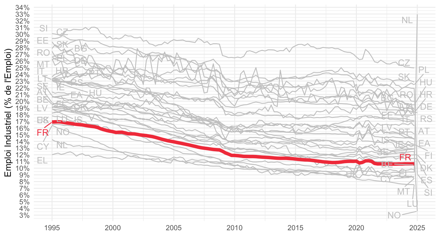
Manufacturing Share
All
Table
Code
namq_10_a10_e %>%
  filter(na_item == "EMP_DC",
         nace_r2 %in% c("C", "TOTAL"),
         s_adj == "SCA",
         unit== "THS_HW",
         time %in% c("2024Q4", "1995Q1", "2024Q3")) %>%
  left_join(geo, by = "geo") %>%
  left_join(nace_r2, by = "nace_r2") %>%
  group_by(time) %>%
  mutate(values = values/ values[nace_r2 == "TOTAL"]) %>%
  filter(nace_r2 != "TOTAL") %>%
  spread(time, values) %>%
  select_if(~ n_distinct(.) > 1) %>%
  mutate(change = `2024Q4`-`1995Q1`) %>%
  arrange(`2024Q3`) %>%
  print_table_conditional()
Table
Code
namq_10_a10_e %>%
  filter(na_item == "EMP_DC",
         nace_r2 %in% c("B-E", "TOTAL"),
         s_adj == "SCA",
         unit== "THS_HW",
         time %in% c("2024Q4", "1995Q1", "2024Q3")) %>%
  left_join(geo, by = "geo") %>%
  left_join(nace_r2, by = "nace_r2") %>%
  group_by(time) %>%
  mutate(values = values/ values[nace_r2 == "TOTAL"]) %>%
  filter(nace_r2 != "TOTAL") %>%
  spread(time, values) %>%
  select_if(~ n_distinct(.) > 1) %>%
  mutate(change = `2024Q4`-`1995Q1`) %>%
  arrange(`2024Q3`) %>%
  print_table_conditional()
1995-
Code
options(ggrepel.max.overlaps = Inf)
namq_10_a10_e %>%
  filter(na_item == "EMP_DC",
         nace_r2 %in% c("C", "TOTAL"),
         s_adj == "SCA",
         unit== "THS_HW") %>%
  quarter_to_date() %>%
  left_join(geo, by = "geo") %>%
  left_join(nace_r2, by = "nace_r2") %>%
  group_by(date) %>%
  mutate(values = values/ values[nace_r2 == "TOTAL"]) %>%
  filter(nace_r2 != "TOTAL",
         date >= as.Date("1995-01-01")) %>%
  mutate(Geo = ifelse(geo == "DE", "Germany", Geo)) %>%
  mutate(Geo = ifelse(geo == "EA", "Europe", Geo)) %>%
  left_join(colors, by = c("Geo" = "country")) %>%
  ggplot(.) + geom_line(aes(x = date, y = values, color = color, group = geo)) +
  scale_color_identity() +
  scale_linetype_manual(values = c("solid", "dashed")) +
  theme_minimal() +
  scale_x_date(breaks = seq(1920, 2100, 5) %>% paste0("-01-01") %>% as.Date,
               labels = date_format("%Y")) +
  theme(legend.position = c(0.2, 0.1),
        legend.title = element_blank()) +
  add_flags(5) +
  scale_y_continuous(breaks = 0.01*seq(-60, 60, 1),
                     labels = scales::percent_format(accuracy = 1)) +
  ylab("Emploi Manufacturier (% de l'Emploi)") + xlab("") +
  geom_line(data = . %>% filter(geo == "FR"),
            aes(x = date, y = values, color = color), size = 2) +
  geom_label_repel(data = . %>% group_by(geo) %>% filter(date %in% c(max(date), min(date))),
            aes(x = date, y = values, color = color, label = geo))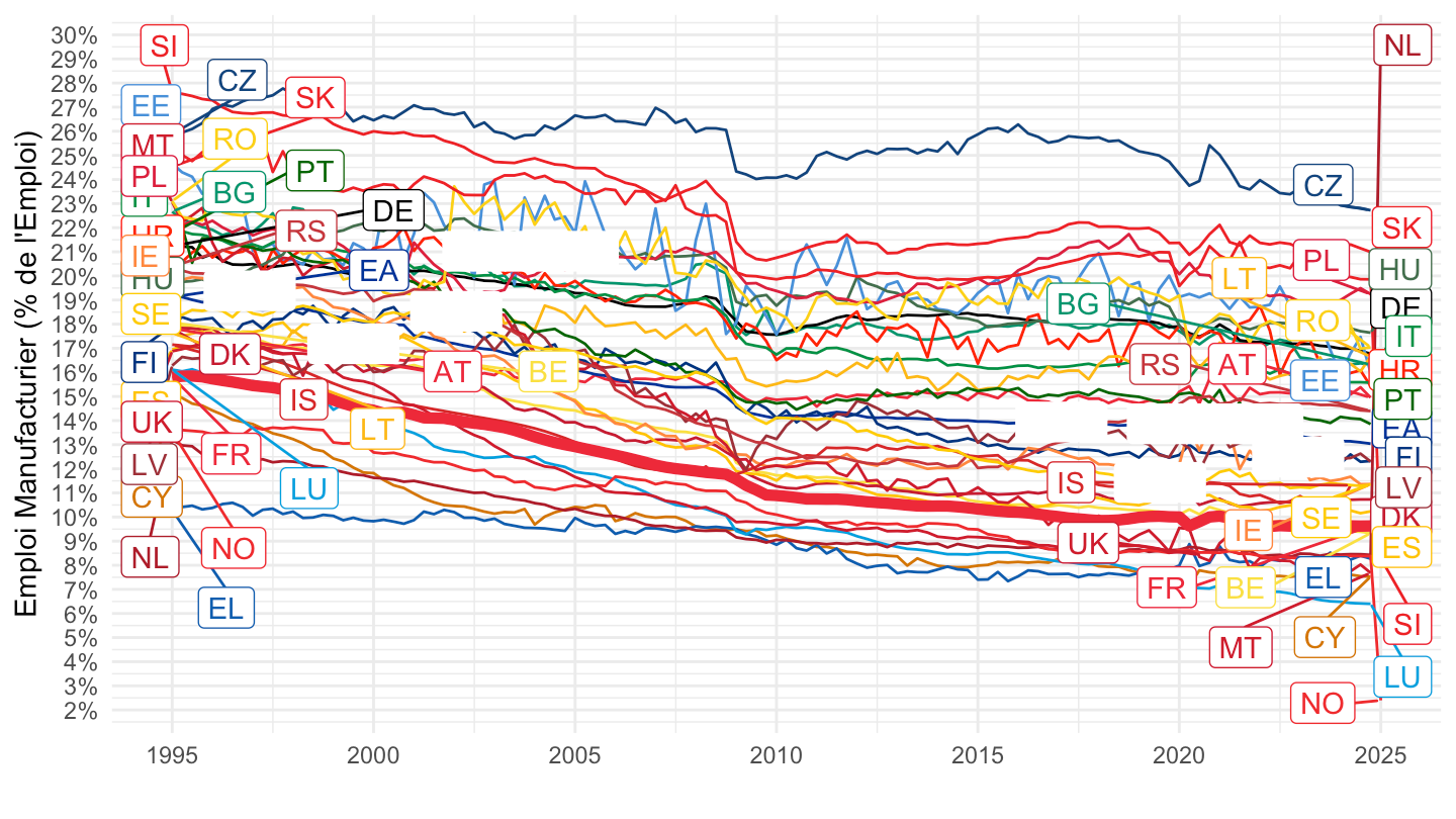
Gris
Code
options(ggrepel.max.overlaps = Inf)
namq_10_a10_e %>%
  filter(na_item == "EMP_DC",
         nace_r2 %in% c("C", "TOTAL"),
         s_adj == "SCA",
         !(geo %in% c("EA12", "EA19", "EA20", "EU27_2020")),
         unit== "THS_HW") %>%
  quarter_to_date() %>%
  left_join(geo, by = "geo") %>%
  left_join(nace_r2, by = "nace_r2") %>%
  group_by(date) %>%
  mutate(values = values/ values[nace_r2 == "TOTAL"]) %>%
  filter(nace_r2 != "TOTAL",
         date >= as.Date("1995-01-01")) %>%
  mutate(Geo = ifelse(geo == "DE", "Germany", Geo)) %>%
  mutate(Geo = ifelse(geo == "EA", "Europe", Geo)) %>%
  left_join(colors, by = c("Geo" = "country")) %>%
  mutate(color = ifelse(geo != "FR", "grey", color)) %>%
  ggplot(.) + geom_line(aes(x = date, y = values, color = color, group = geo)) +
  scale_color_identity() +
  scale_linetype_manual(values = c("solid", "dashed")) +
  theme_minimal() +
  scale_x_date(breaks = seq(1920, 2100, 5) %>% paste0("-01-01") %>% as.Date,
               labels = date_format("%Y")) +
  theme(legend.position = c(0.2, 0.1),
        legend.title = element_blank()) +
  add_flags(5) +
  scale_y_continuous(breaks = 0.01*seq(-60, 60, 1),
                     labels = scales::percent_format(accuracy = 1)) +
  ylab("Emploi manufacturier (% de l'Emploi)") + xlab("") +
  geom_line(data = . %>% filter(geo == "FR"),
            aes(x = date, y = values, color = color), size = 2) +
  geom_text_repel(data = . %>% group_by(geo) %>% filter(date %in% c(max(date), min(date))),
            aes(x = date, y = values, color = color, label = geo))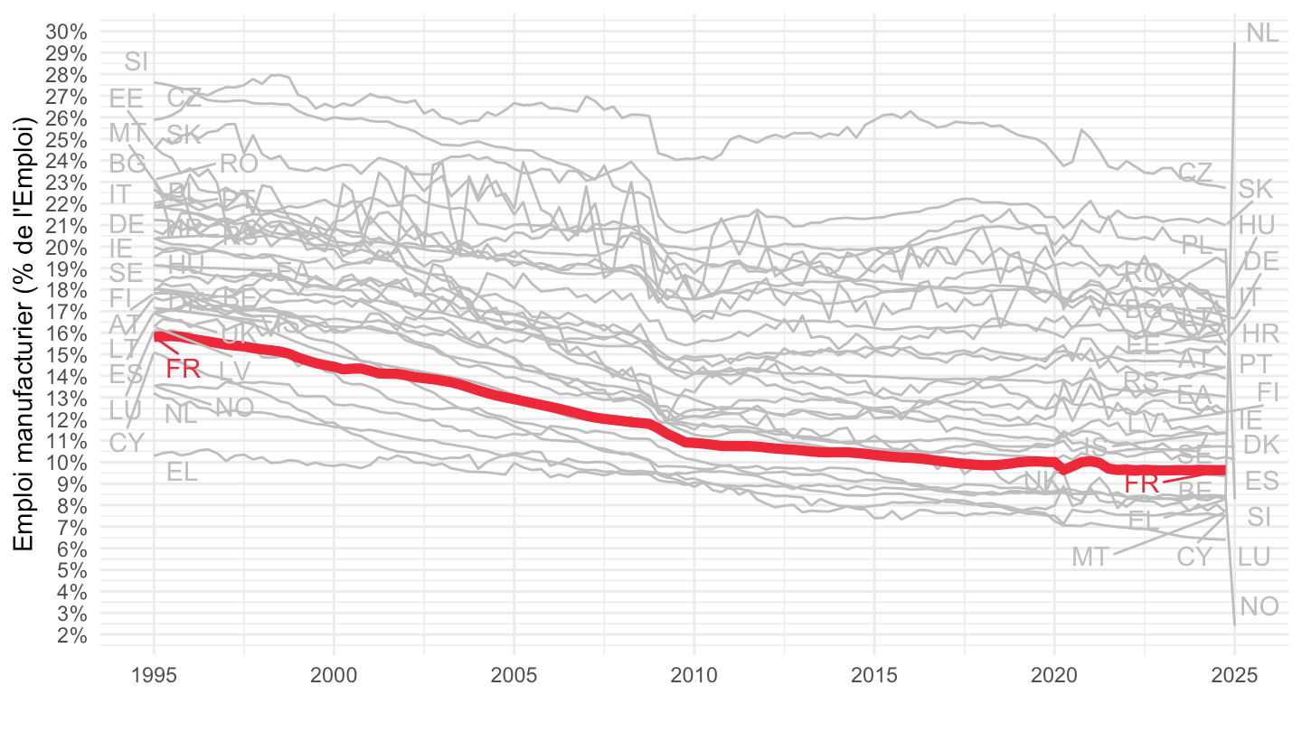
France, Germany, Italy, Spain, Netherlands, Euro area
1995-
Code
namq_10_a10_e %>%
  filter(na_item == "EMP_DC",
         nace_r2 %in% c("C", "TOTAL"),
         geo %in% c("FR", "DE", "IT", "ES", "EA"),
         s_adj == "SCA",
         unit== "THS_HW") %>%
  quarter_to_date() %>%
  left_join(geo, by = "geo") %>%
  left_join(nace_r2, by = "nace_r2") %>%
  group_by(date) %>%
  mutate(values = values/ values[nace_r2 == "TOTAL"]) %>%
  filter(nace_r2 != "TOTAL",
         date >= as.Date("1995-01-01")) %>%
  mutate(Geo = ifelse(geo == "DE", "Germany", Geo)) %>%
  mutate(Geo = ifelse(geo == "EA", "Europe", Geo)) %>%
  left_join(colors, by = c("Geo" = "country")) %>%
  ggplot(.) + geom_line(aes(x = date, y = values, color = color)) +
  scale_color_identity() +
  scale_linetype_manual(values = c("solid", "dashed")) +
  theme_minimal() +
  scale_x_date(breaks = seq(1920, 2100, 5) %>% paste0("-01-01") %>% as.Date,
               labels = date_format("%Y")) +
  theme(legend.position = c(0.2, 0.1),
        legend.title = element_blank()) +
  add_flags(5) +
  scale_y_continuous(breaks = 0.01*seq(-60, 60, 1),
                     labels = scales::percent_format(accuracy = 1)) +
  ylab("Emploi Manufacturier (% de l'Emploi)") + xlab("")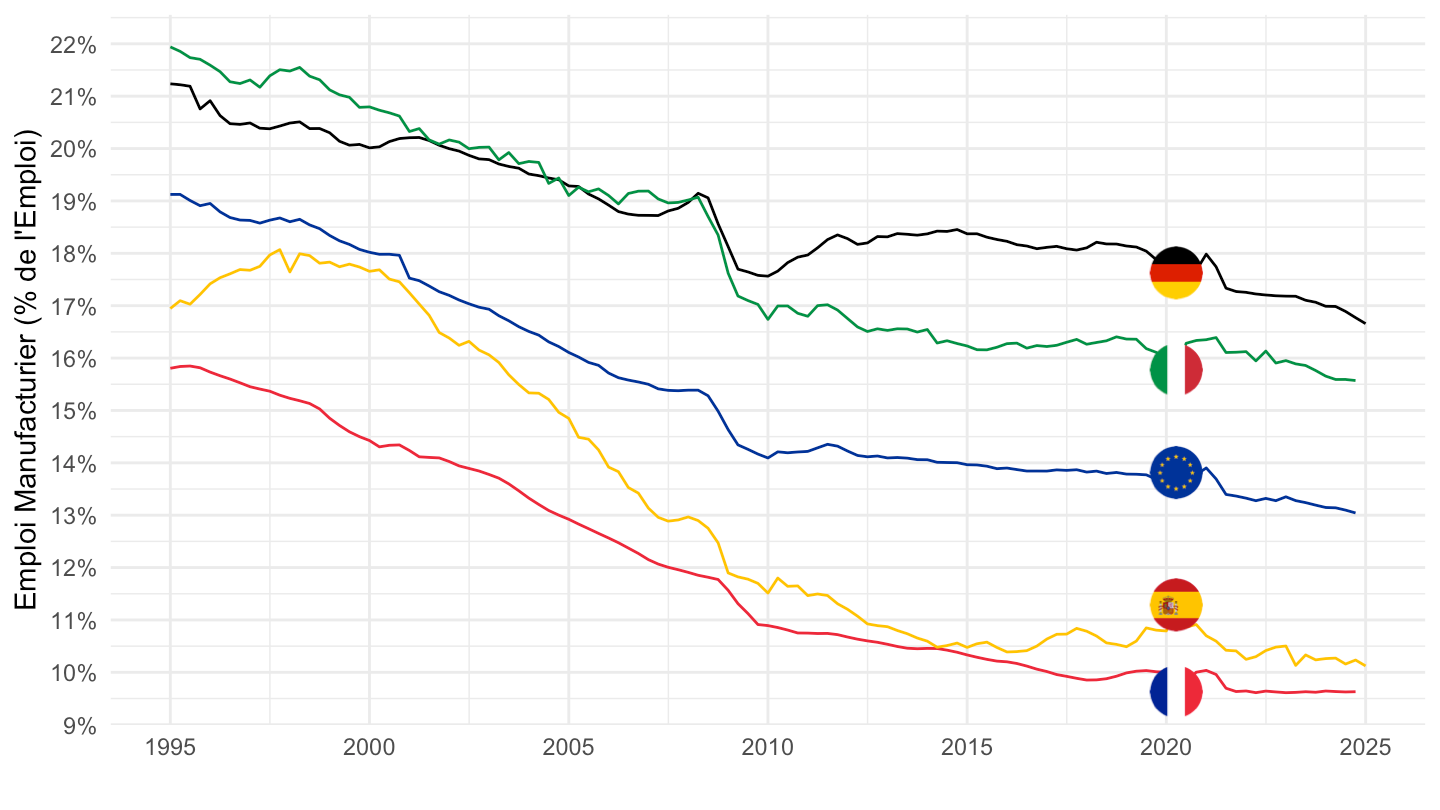
Industry and Manufacturing Share
France, Germany, Italy, Romania
1995-
Code
load_data("eurostat/nace_r2_fr.RData")
namq_10_a10_e %>%
  filter(na_item == "EMP_DC",
         nace_r2 %in% c("C", "TOTAL", "B-E"),
         geo %in% c("FR", "DE", "IT", "RO"),
         s_adj == "SCA",
         unit== "THS_HW") %>%
  quarter_to_date() %>%
  left_join(geo, by = "geo") %>%
  left_join(nace_r2, by = "nace_r2") %>%
  group_by(date) %>%
  mutate(values = values/ values[nace_r2 == "TOTAL"]) %>%
  filter(nace_r2 != "TOTAL",
         date >= as.Date("1995-01-01")) %>%
  mutate(Geo = ifelse(geo == "DE", "Germany", Geo)) %>%
  left_join(colors, by = c("Geo" = "country")) %>%
  ggplot(.) + geom_line(aes(x = date, y = values, color = color, linetype = Nace_r2)) +
  scale_color_identity() +
  scale_linetype_manual(values = c("solid", "dashed")) +
  theme_minimal() +
  scale_x_date(breaks = seq(1920, 2100, 2) %>% paste0("-01-01") %>% as.Date,
               labels = date_format("%Y")) +
  theme(legend.position = c(0.2, 0.1),
        legend.title = element_blank()) +
  add_8flags +
  scale_y_continuous(breaks = 0.01*seq(-60, 60, 1),
                     labels = scales::percent_format(accuracy = 1)) +
  ylab("Emploi Manufacturier, Industriel (% de l'Emploi)") + xlab("")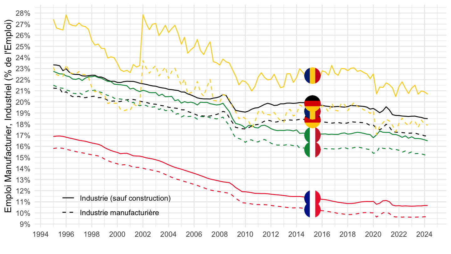
France, Germany, Italy
1995-
Code
load_data("eurostat/nace_r2_fr.RData")
namq_10_a10_e %>%
  filter(na_item == "EMP_DC",
         nace_r2 %in% c("C", "TOTAL", "B-E"),
         geo %in% c("FR", "DE", "IT"),
         s_adj == "SCA",
         unit== "THS_HW") %>%
  quarter_to_date() %>%
  left_join(geo, by = "geo") %>%
  left_join(nace_r2, by = "nace_r2") %>%
  group_by(date) %>%
  mutate(values = values/ values[nace_r2 == "TOTAL"]) %>%
  filter(nace_r2 != "TOTAL",
         date >= as.Date("1995-01-01")) %>%
  mutate(Geo = ifelse(geo == "DE", "Germany", Geo)) %>%
  left_join(colors, by = c("Geo" = "country")) %>%
  ggplot(.) + geom_line(aes(x = date, y = values, color = color, linetype = Nace_r2)) +
  scale_color_identity() +
  scale_linetype_manual(values = c("solid", "dashed")) +
  theme_minimal() +
  scale_x_date(breaks = seq(1920, 2100, 2) %>% paste0("-01-01") %>% as.Date,
               labels = date_format("%Y")) +
  theme(legend.position = c(0.2, 0.1),
        legend.title = element_blank()) +
  add_6flags +
  scale_y_continuous(breaks = 0.01*seq(-60, 60, 1),
                     labels = scales::percent_format(accuracy = 1)) +
  ylab("Emploi Manufacturier, Industriel (% de l'Emploi)") + xlab("")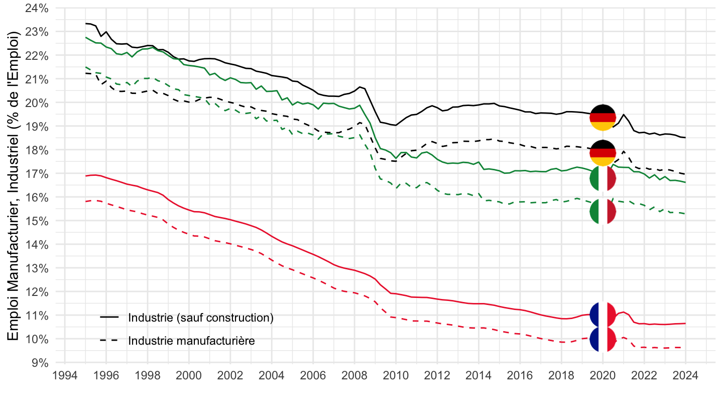
2008-
Code
namq_10_a10_e %>%
  filter(na_item == "EMP_DC",
         nace_r2 %in% c("C", "TOTAL", "B-E"),
         geo %in% c("FR", "DE", "IT"),
         s_adj == "SCA",
         unit== "THS_HW") %>%
  quarter_to_date() %>%
  left_join(geo, by = "geo") %>%
  left_join(nace_r2, by = "nace_r2") %>%
  group_by(date) %>%
  mutate(values = values/ values[nace_r2 == "TOTAL"]) %>%
  filter(nace_r2 != "TOTAL",
         date >= as.Date("2008-01-01")) %>%
  left_join(colors, by = c("Geo" = "country")) %>%
  mutate(Geo = ifelse(geo == "DE", "Germany", Geo)) %>%
  ggplot(.) + geom_line(aes(x = date, y = values, color = color, linetype = Nace_r2)) +
  scale_color_identity() +
  scale_linetype_manual(values = c("solid", "dashed")) +
  theme_minimal() +
  scale_x_date(breaks = seq(1920, 2100, 2) %>% paste0("-01-01") %>% as.Date,
               labels = date_format("%Y")) +
  theme(legend.position = c(0.2, 0.5),
        legend.title = element_blank()) +
  add_6flags +
  scale_y_continuous(breaks = 0.01*seq(-60, 60, 1),
                     labels = scales::percent_format(accuracy = 1)) +
  ylab("Emploi Manufacturier, Industriel (% de l'Emploi)") + xlab("")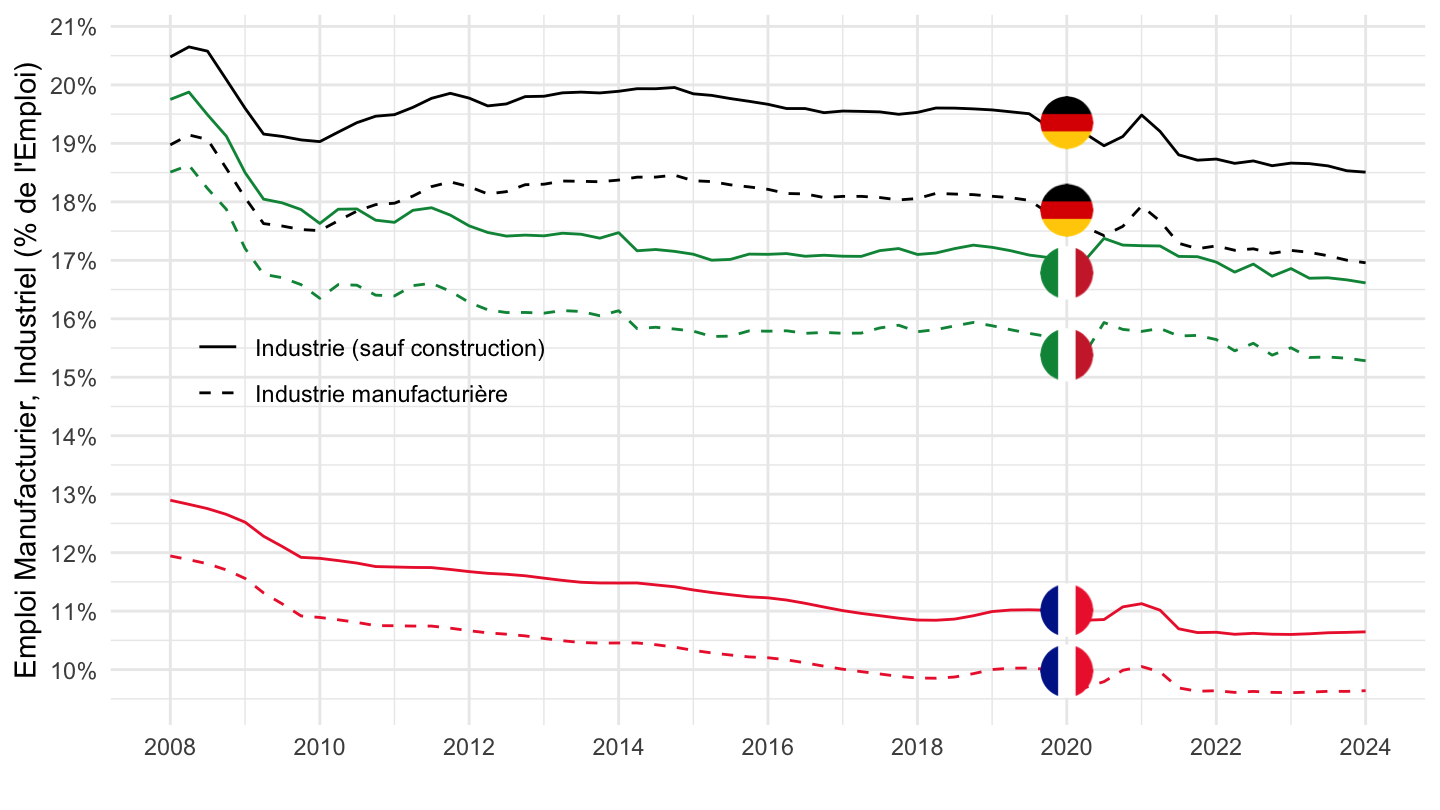
France, Germany, Italy, Spain, Netherlands, Euro area
1995-
Code
namq_10_a10_e %>%
  filter(na_item == "EMP_DC",
         nace_r2 %in% c("C", "TOTAL", "B-E"),
         geo %in% c("FR", "DE", "IT", "ES", "EA"),
         s_adj == "SCA",
         unit== "THS_HW") %>%
  quarter_to_date() %>%
  left_join(geo, by = "geo") %>%
  left_join(nace_r2, by = "nace_r2") %>%
  group_by(date) %>%
  mutate(values = values/ values[nace_r2 == "TOTAL"]) %>%
  filter(nace_r2 != "TOTAL",
         date >= as.Date("1995-01-01")) %>%
  mutate(Geo = ifelse(geo == "DE", "Germany", Geo)) %>%
  mutate(Geo = ifelse(geo == "EA", "Europe", Geo)) %>%
  left_join(colors, by = c("Geo" = "country")) %>%
  ggplot(.) + geom_line(aes(x = date, y = values, color = color, linetype = Nace_r2)) +
  scale_color_identity() +
  scale_linetype_manual(values = c("solid", "dashed")) +
  theme_minimal() +
  scale_x_date(breaks = seq(1920, 2100, 2) %>% paste0("-01-01") %>% as.Date,
               labels = date_format("%Y")) +
  theme(legend.position = c(0.2, 0.1),
        legend.title = element_blank()) +
  add_flags(10) +
  scale_y_continuous(breaks = 0.01*seq(-60, 60, 1),
                     labels = scales::percent_format(accuracy = 1)) +
  ylab("Emploi Manufacturier, Industriel (% de l'Emploi)") + xlab("")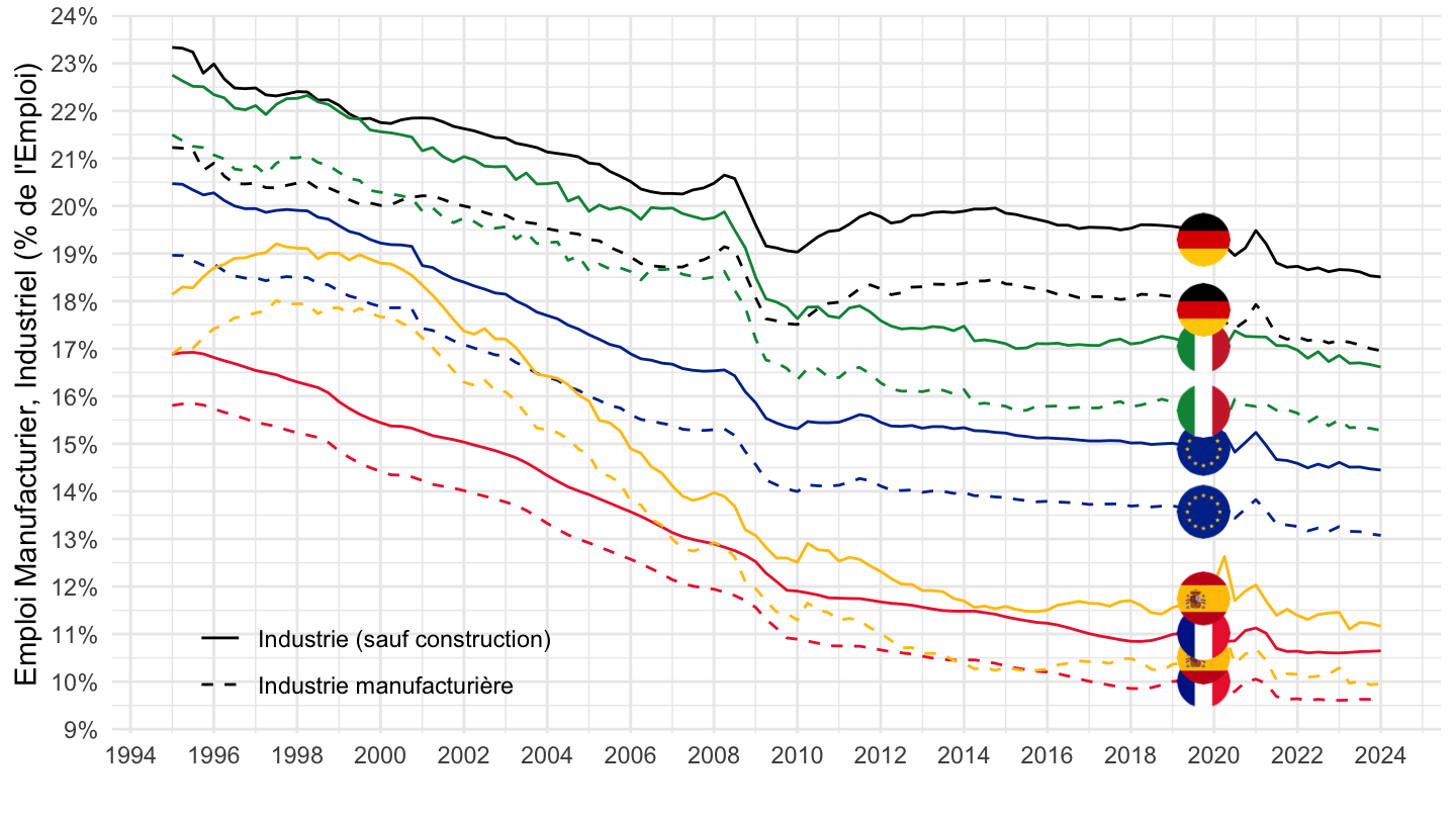
2008-
Code
namq_10_a10_e %>%
  filter(na_item == "EMP_DC",
         nace_r2 %in% c("C", "TOTAL", "B-E"),
         geo %in% c("FR", "DE", "IT", "ES", "EA"),
         s_adj == "SCA",
         unit== "THS_HW") %>%
  quarter_to_date() %>%
  left_join(geo, by = "geo") %>%
  left_join(nace_r2, by = "nace_r2") %>%
  group_by(date) %>%
  mutate(values = values/ values[nace_r2 == "TOTAL"]) %>%
  filter(nace_r2 != "TOTAL",
         date >= as.Date("2008-01-01")) %>%
  mutate(Geo = ifelse(geo == "DE", "Germany", Geo)) %>%
  mutate(Geo = ifelse(geo == "EA", "Europe", Geo)) %>%
  left_join(colors, by = c("Geo" = "country")) %>%
  ggplot(.) + geom_line(aes(x = date, y = values, color = color, linetype = Nace_r2)) +
  scale_color_identity() +
  scale_linetype_manual(values = c("solid", "dashed")) +
  theme_minimal() +
  scale_x_date(breaks = seq(1920, 2100, 2) %>% paste0("-01-01") %>% as.Date,
               labels = date_format("%Y")) +
  theme(legend.position = c(0.3, 0.9),
        legend.title = element_blank()) +
  add_flags(10) +
  scale_y_continuous(breaks = 0.01*seq(-60, 60, 1),
                     labels = scales::percent_format(accuracy = 1)) +
  ylab("Emploi Manufacturier, Industriel (% de l'Emploi)") + xlab("")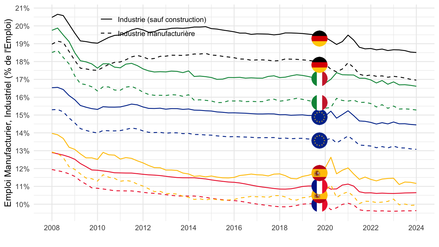
2017-
Code
namq_10_a10_e %>%
  filter(na_item == "EMP_DC",
         nace_r2 %in% c("C", "TOTAL", "B-E"),
         geo %in% c("FR", "DE", "IT", "ES", "EA"),
         s_adj == "SCA",
         unit== "THS_HW") %>%
  quarter_to_date() %>%
  left_join(geo, by = "geo") %>%
  left_join(nace_r2, by = "nace_r2") %>%
  group_by(date) %>%
  mutate(values = values/ values[nace_r2 == "TOTAL"]) %>%
  filter(nace_r2 != "TOTAL",
         date >= as.Date("2017-01-01")) %>%
  mutate(Geo = ifelse(geo == "DE", "Germany", Geo)) %>%
  mutate(Geo = ifelse(geo == "EA", "Europe", Geo)) %>%
  left_join(colors, by = c("Geo" = "country")) %>%
  ggplot(.) + geom_line(aes(x = date, y = values, color = color, linetype = Nace_r2)) +
  scale_color_identity() +
  scale_linetype_manual(values = c("solid", "dashed")) +
  theme_minimal() +
  scale_x_date(breaks = seq(1920, 2100, 1) %>% paste0("-01-01") %>% as.Date,
               labels = date_format("%Y")) +
  theme(legend.position = c(0.3, 0.9),
        legend.title = element_blank()) +
  add_flags(10) +
  scale_y_continuous(breaks = 0.01*seq(-60, 60, 1),
                     labels = scales::percent_format(accuracy = 1)) +
  ylab("Emploi Manufacturier, Industriel (% de l'Emploi)") + xlab("")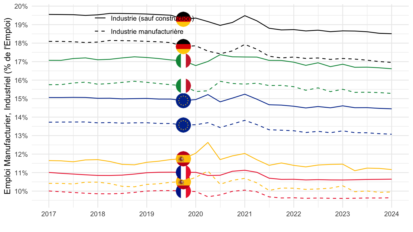
Spain, Netherlands, Portugal
1995-
Code
namq_10_a10_e %>%
  filter(na_item == "EMP_DC",
         nace_r2 %in% c("C", "TOTAL", "B-E"),
         geo %in% c("ES", "NL", "PT"),
         s_adj == "SCA",
         unit== "THS_HW") %>%
  quarter_to_date() %>%
  left_join(geo, by = "geo") %>%
  left_join(nace_r2, by = "nace_r2") %>%
  group_by(date) %>%
  mutate(values = values/ values[nace_r2 == "TOTAL"]) %>%
  filter(nace_r2 != "TOTAL",
         date >= as.Date("1995-01-01")) %>%
  left_join(colors, by = c("Geo" = "country")) %>%
  mutate(Geo = ifelse(geo == "DE", "Germany", Geo)) %>%
  ggplot(.) + geom_line(aes(x = date, y = values, color = color, linetype = Nace_r2)) +
  scale_color_identity() +
  scale_linetype_manual(values = c("solid", "dashed")) +
  theme_minimal() +
  scale_x_date(breaks = seq(1920, 2100, 5) %>% paste0("-01-01") %>% as.Date,
               labels = date_format("%Y")) +
  theme(legend.position = c(0.7, 0.8),
        legend.title = element_blank()) +
  add_6flags +
  scale_y_continuous(breaks = 0.01*seq(-60, 60, 2),
                     labels = scales::percent_format(accuracy = 1)) +
  ylab("Emploi Manufacturier, Industriel (% de l'Emploi)") + xlab("")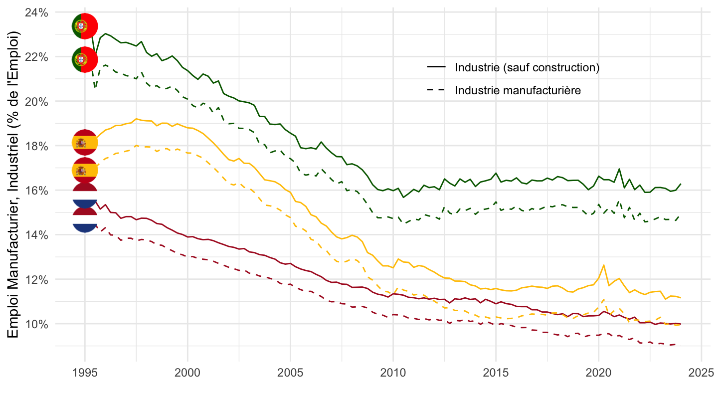
2008-
Code
namq_10_a10_e %>%
  filter(na_item == "EMP_DC",
         nace_r2 %in% c("C", "TOTAL", "B-E"),
         geo %in% c("ES", "NL", "PT"),
         s_adj == "SCA",
         unit== "THS_HW") %>%
  quarter_to_date() %>%
  left_join(geo, by = "geo") %>%
  left_join(nace_r2, by = "nace_r2") %>%
  group_by(date) %>%
  mutate(values = values/ values[nace_r2 == "TOTAL"]) %>%
  filter(nace_r2 != "TOTAL",
         date >= as.Date("2008-01-01")) %>%
  left_join(colors, by = c("Geo" = "country")) %>%
  mutate(Geo = ifelse(geo == "DE", "Germany", Geo)) %>%
  ggplot(.) + geom_line(aes(x = date, y = values, color = color, linetype = Nace_r2)) +
  scale_color_identity() +
  scale_linetype_manual(values = c("solid", "dashed")) +
  theme_minimal() +
  scale_x_date(breaks = seq(1920, 2100, 2) %>% paste0("-01-01") %>% as.Date,
               labels = date_format("%Y")) +
  theme(legend.position = c(0.2, 0.5),
        legend.title = element_blank()) +
  add_6flags +
  scale_y_continuous(breaks = 0.01*seq(-60, 60, 1),
                     labels = scales::percent_format(accuracy = 1)) +
  ylab("Emploi Manufacturier, Industriel (% de l'Emploi)") + xlab("")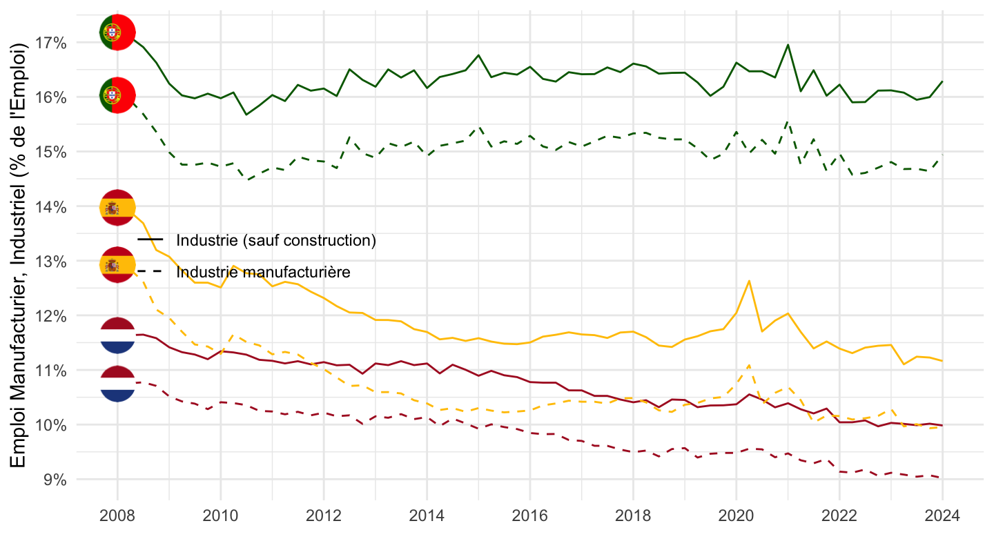
% of Total Employment
France
Code
load_data("eurostat/nace_r2.RData")
namq_10_a10_e %>%
  filter(na_item == "EMP_DC",
         nace_r2 %in% c("C", "TOTAL", "L", "F"),
         geo %in% c("FR"),
         s_adj == "SCA",
         unit== "THS_HW") %>%
  quarter_to_date() %>%
  left_join(nace_r2, by = "nace_r2") %>%
  select(nace_r2, Nace_r2, date, values) %>%
  group_by(date) %>%
  mutate(values = values/ values[nace_r2 == "TOTAL"]) %>%
  filter(nace_r2 != "TOTAL")  %>%
  ggplot(.) + geom_line(aes(x = date, y = values, color = Nace_r2)) +
  theme_minimal() + xlab("") + ylab("% of Employment") +
  scale_color_manual(values = viridis(4)[1:3]) +
  scale_x_date(breaks = seq(1960, 2100, 5) %>% paste0("-01-01") %>% as.Date,
               labels = date_format("%Y")) +
  scale_y_continuous(breaks = 0.01*seq(-500, 200, 1),
                     labels = percent_format(accuracy = 1)) +
  theme(legend.position = c(0.75, 0.85),
        legend.title = element_blank())
Germany
Code
namq_10_a10_e %>%
  filter(na_item == "EMP_DC",
         nace_r2 %in% c("C", "TOTAL", "L", "F"),
         geo %in% c("DE"),
         s_adj == "SCA",
         unit== "THS_HW") %>%
  quarter_to_date() %>%
  left_join(nace_r2, by = "nace_r2") %>%
  select(nace_r2, Nace_r2, date, values) %>%
  group_by(date) %>%
  mutate(values = values/ values[nace_r2 == "TOTAL"]) %>%
  filter(nace_r2 != "TOTAL")  %>%
  ggplot(.) + geom_line(aes(x = date, y = values, color = Nace_r2)) +
  theme_minimal() + xlab("") + ylab("% of Employment") +
  scale_color_manual(values = viridis(4)[1:3]) +
  scale_x_date(breaks = seq(1960, 2100, 5) %>% paste0("-01-01") %>% as.Date,
               labels = date_format("%Y")) +
  scale_y_continuous(breaks = 0.01*seq(-500, 200, 1),
                     labels = percent_format(accuracy = 1)) +
  theme(legend.position = c(0.75, 0.85),
        legend.title = element_blank())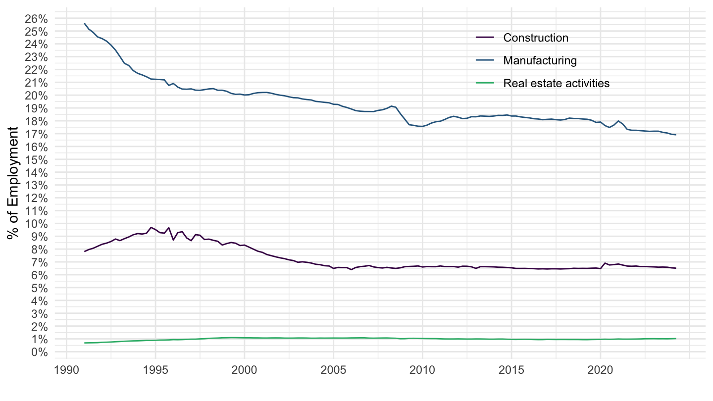
Italy
Code
namq_10_a10_e %>%
  filter(na_item == "EMP_DC",
         nace_r2 %in% c("C", "TOTAL", "L", "F"),
         geo %in% c("IT"),
         s_adj == "SCA",
         unit== "THS_HW") %>%
  quarter_to_date() %>%
  left_join(nace_r2, by = "nace_r2") %>%
  select(nace_r2, Nace_r2, date, values) %>%
  group_by(date) %>%
  mutate(values = values/ values[nace_r2 == "TOTAL"]) %>%
  filter(nace_r2 != "TOTAL")  %>%
  ggplot(.) + geom_line(aes(x = date, y = values, color = Nace_r2)) +
  theme_minimal() + xlab("") + ylab("% of Employment") +
  scale_color_manual(values = viridis(4)[1:3]) +
  scale_x_date(breaks = seq(1960, 2100, 5) %>% paste0("-01-01") %>% as.Date,
               labels = date_format("%Y")) +
  scale_y_continuous(breaks = 0.01*seq(-500, 200, 1),
                     labels = percent_format(accuracy = 1)) +
  theme(legend.position = c(0.75, 0.85),
        legend.title = element_blank())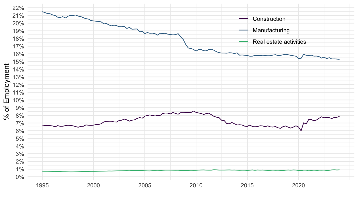
Spain
Code
namq_10_a10_e %>%
  filter(na_item == "EMP_DC",
         nace_r2 %in% c("C", "TOTAL", "L", "F"),
         geo %in% c("ES"),
         s_adj == "SCA",
         unit== "THS_HW") %>%
  quarter_to_date() %>%
  left_join(nace_r2, by = "nace_r2") %>%
  select(nace_r2, Nace_r2, date, values) %>%
  group_by(date) %>%
  mutate(values = values/ values[nace_r2 == "TOTAL"]) %>%
  filter(nace_r2 != "TOTAL")  %>%
  ggplot(.) + geom_line(aes(x = date, y = values, color = Nace_r2)) +
  theme_minimal() + xlab("") + ylab("% of Employment") +
  scale_color_manual(values = viridis(4)[1:3]) +
  scale_x_date(breaks = seq(1960, 2100, 5) %>% paste0("-01-01") %>% as.Date,
               labels = date_format("%Y")) +
  scale_y_continuous(breaks = 0.01*seq(-500, 200, 1),
                     labels = percent_format(accuracy = 1)) +
  theme(legend.position = c(0.75, 0.85),
        legend.title = element_blank())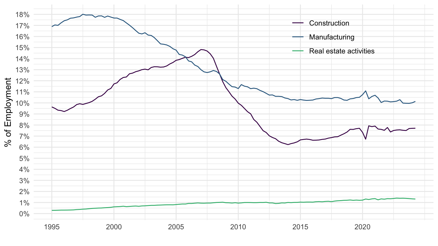
Greece
Code
namq_10_a10_e %>%
  filter(na_item == "EMP_DC",
         nace_r2 %in% c("C", "TOTAL", "L", "F"),
         geo %in% c("EL"),
         s_adj == "SCA",
         unit== "THS_HW") %>%
  quarter_to_date() %>%
  left_join(nace_r2, by = "nace_r2") %>%
  select(nace_r2, Nace_r2, date, values) %>%
  group_by(date) %>%
  mutate(values = values/ values[nace_r2 == "TOTAL"]) %>%
  filter(nace_r2 != "TOTAL")  %>%
  ggplot(.) + geom_line(aes(x = date, y = values, color = Nace_r2)) +
  theme_minimal() + xlab("") + ylab("% of Employment") +
  scale_color_manual(values = viridis(4)[1:3]) +
  scale_x_date(breaks = seq(1960, 2100, 5) %>% paste0("-01-01") %>% as.Date,
               labels = date_format("%Y")) +
  scale_y_continuous(breaks = 0.01*seq(-500, 200, 1),
                     labels = percent_format(accuracy = 1)) +
  theme(legend.position = c(0.8, 0.9),
        legend.title = element_blank())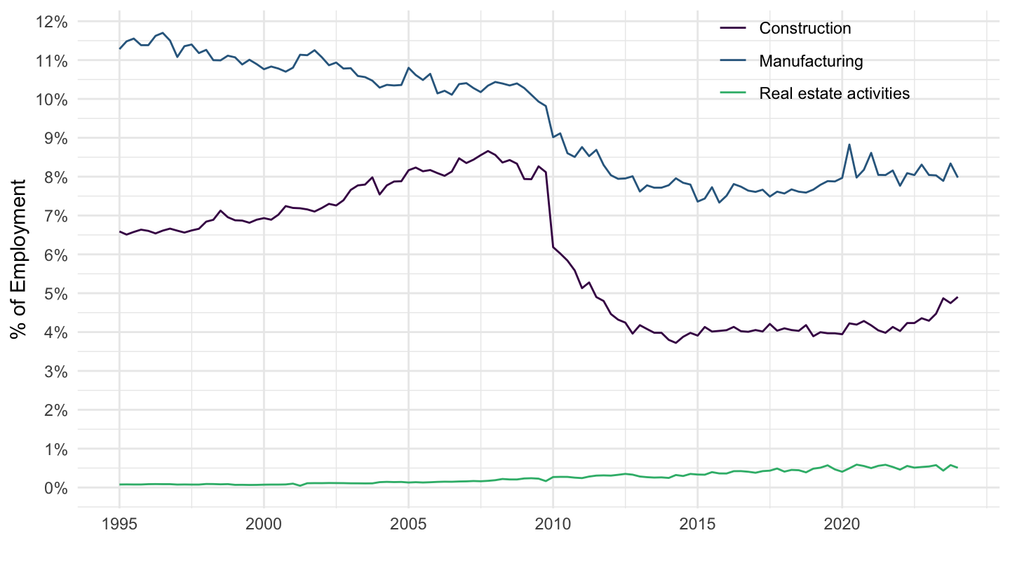
Netherlands
Code
namq_10_a10_e %>%
  filter(na_item == "EMP_DC",
         nace_r2 %in% c("C", "TOTAL", "L", "F"),
         geo %in% c("NL"),
         s_adj == "SCA",
         unit== "THS_HW") %>%
  quarter_to_date() %>%
  left_join(nace_r2, by = "nace_r2") %>%
  select(nace_r2, Nace_r2, date, values) %>%
  group_by(date) %>%
  mutate(values = values/ values[nace_r2 == "TOTAL"]) %>%
  filter(nace_r2 != "TOTAL")  %>%
  ggplot(.) + geom_line(aes(x = date, y = values, color = Nace_r2)) +
  theme_minimal() + xlab("") + ylab("% of Employment") +
  scale_color_manual(values = viridis(4)[1:3]) +
  scale_x_date(breaks = seq(1960, 2100, 5) %>% paste0("-01-01") %>% as.Date,
               labels = date_format("%Y")) +
  scale_y_continuous(breaks = 0.01*seq(-500, 200, 1),
                     labels = percent_format(accuracy = 1)) +
  theme(legend.position = c(0.8, 0.9),
        legend.title = element_blank())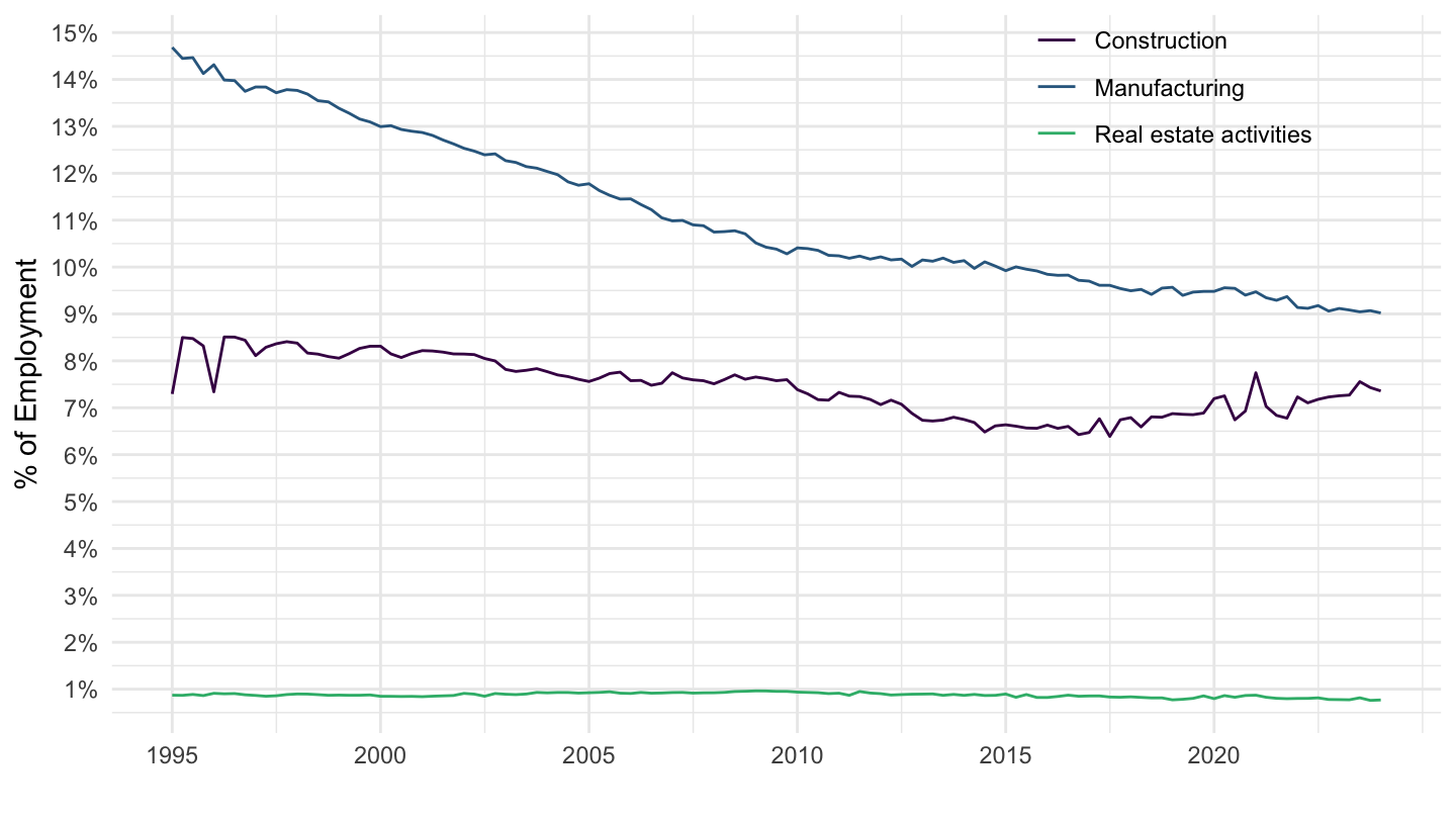
Denmark
Code
namq_10_a10_e %>%
  filter(na_item == "EMP_DC",
         nace_r2 %in% c("C", "TOTAL", "L", "F"),
         geo %in% c("DK"),
         s_adj == "SCA",
         unit== "THS_HW") %>%
  quarter_to_date() %>%
  left_join(nace_r2, by = "nace_r2") %>%
  select(nace_r2, Nace_r2, date, values) %>%
  group_by(date) %>%
  mutate(values = values/ values[nace_r2 == "TOTAL"]) %>%
  filter(nace_r2 != "TOTAL")  %>%
  ggplot(.) + geom_line(aes(x = date, y = values, color = Nace_r2)) +
  theme_minimal() + xlab("") + ylab("% of Employment") +
  scale_color_manual(values = viridis(4)[1:3]) +
  scale_x_date(breaks = seq(1960, 2100, 5) %>% paste0("-01-01") %>% as.Date,
               labels = date_format("%Y")) +
  scale_y_continuous(breaks = 0.01*seq(-500, 200, 1),
                     labels = percent_format(accuracy = 1)) +
  theme(legend.position = c(0.8, 0.9),
        legend.title = element_blank())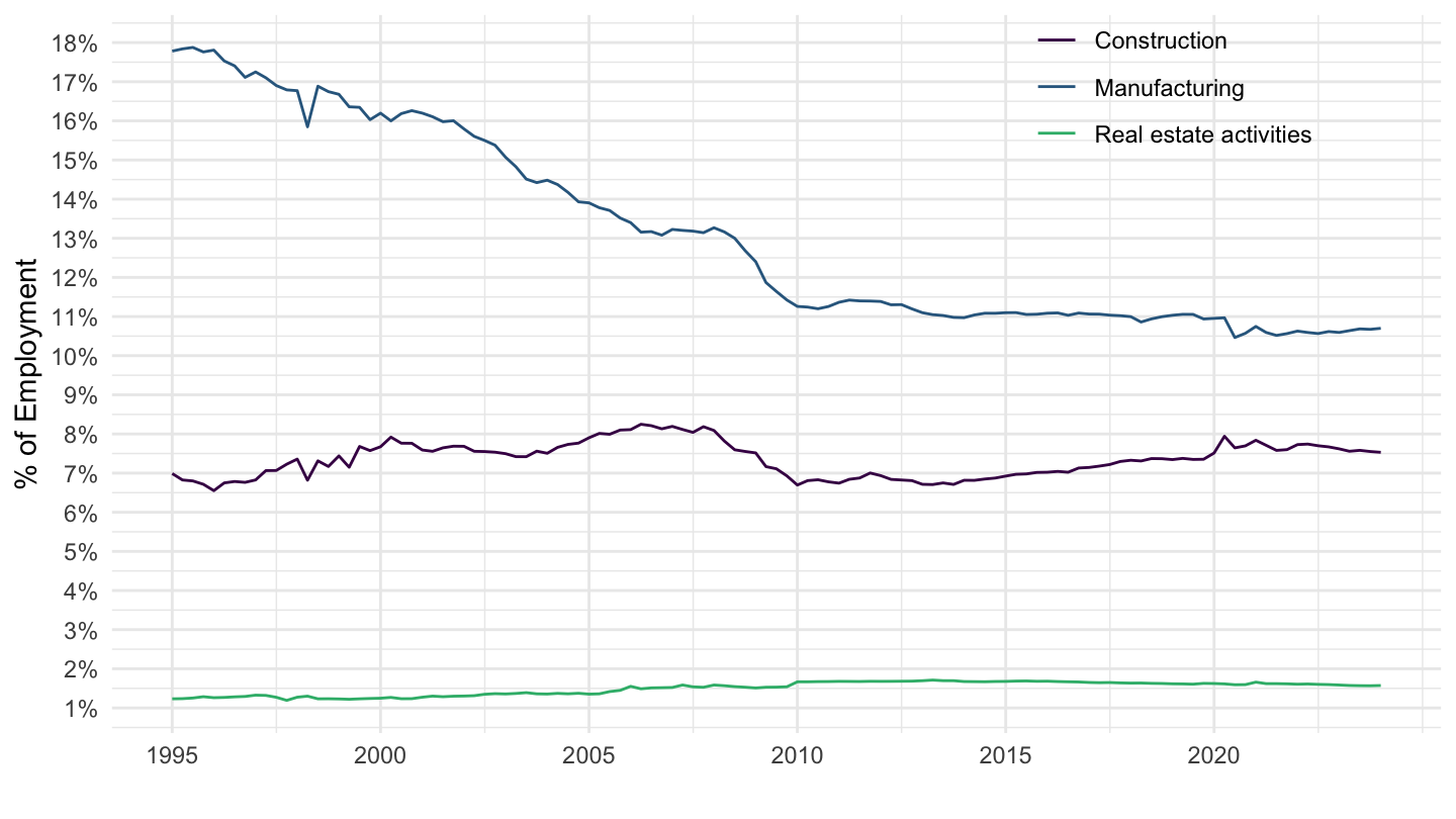
Finland
Code
namq_10_a10_e %>%
  filter(na_item == "EMP_DC",
         nace_r2 %in% c("C", "TOTAL", "L", "F"),
         geo %in% c("FI"),
         s_adj == "SCA",
         unit== "THS_HW") %>%
  quarter_to_date() %>%
  left_join(nace_r2, by = "nace_r2") %>%
  select(nace_r2, Nace_r2, date, values) %>%
  group_by(date) %>%
  mutate(values = values/ values[nace_r2 == "TOTAL"]) %>%
  filter(nace_r2 != "TOTAL")  %>%
  ggplot(.) + geom_line(aes(x = date, y = values, color = Nace_r2)) +
  theme_minimal() + xlab("") + ylab("% of Employment") +
  scale_color_manual(values = viridis(4)[1:3]) +
  scale_x_date(breaks = seq(1960, 2100, 5) %>% paste0("-01-01") %>% as.Date,
               labels = date_format("%Y")) +
  scale_y_continuous(breaks = 0.01*seq(-500, 200, 1),
                     labels = percent_format(accuracy = 1)) +
  theme(legend.position = c(0.8, 0.9),
        legend.title = element_blank())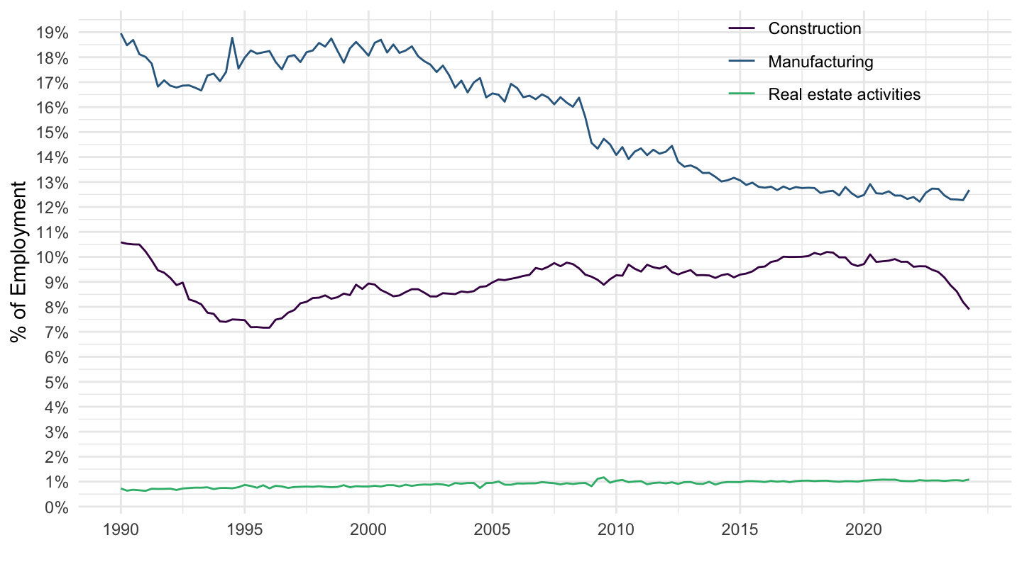
Poland
Code
namq_10_a10_e %>%
  filter(na_item == "EMP_DC",
         nace_r2 %in% c("C", "TOTAL", "L", "F"),
         geo %in% c("PL"),
         s_adj == "SCA",
         unit== "THS_HW") %>%
  quarter_to_date() %>%
  left_join(nace_r2, by = "nace_r2") %>%
  select(nace_r2, Nace_r2, date, values) %>%
  group_by(date) %>%
  mutate(values = values/ values[nace_r2 == "TOTAL"]) %>%
  filter(nace_r2 != "TOTAL")  %>%
  ggplot(.) + geom_line(aes(x = date, y = values, color = Nace_r2)) +
  theme_minimal() + xlab("") + ylab("% of Employment") +
  scale_color_manual(values = viridis(4)[1:3]) +
  scale_x_date(breaks = seq(1960, 2100, 5) %>% paste0("-01-01") %>% as.Date,
               labels = date_format("%Y")) +
  scale_y_continuous(breaks = 0.01*seq(-500, 200, 1),
                     labels = percent_format(accuracy = 1)) +
  theme(legend.position = c(0.8, 0.9),
        legend.title = element_blank())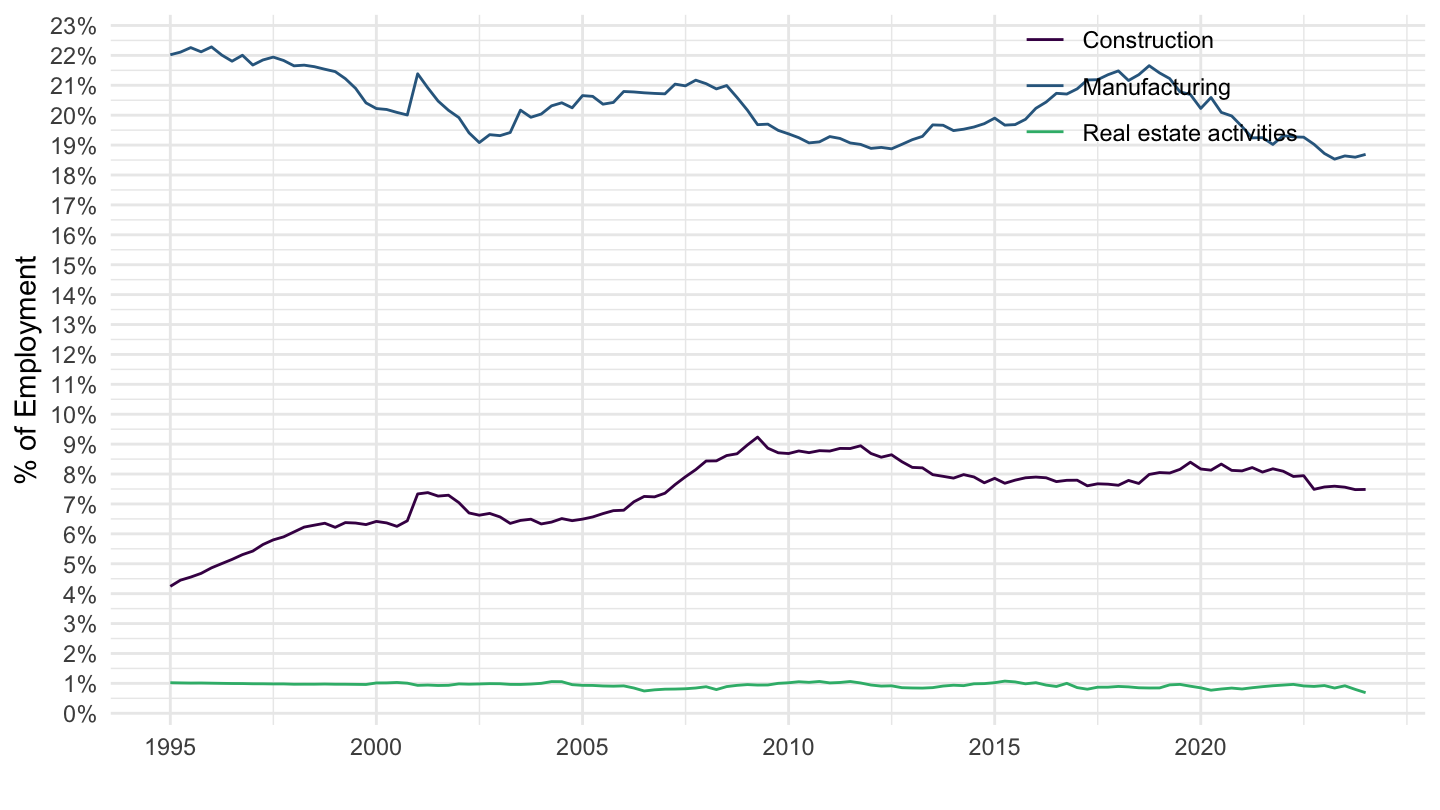
Hungary
Code
namq_10_a10_e %>%
  filter(na_item == "EMP_DC",
         nace_r2 %in% c("C", "TOTAL", "L", "F"),
         geo %in% c("HU"),
         s_adj == "SCA",
         unit== "THS_HW") %>%
  quarter_to_date() %>%
  left_join(nace_r2, by = "nace_r2") %>%
  select(nace_r2, Nace_r2, date, values) %>%
  group_by(date) %>%
  mutate(values = values/ values[nace_r2 == "TOTAL"]) %>%
  filter(nace_r2 != "TOTAL")  %>%
  ggplot(.) + geom_line(aes(x = date, y = values, color = Nace_r2)) +
  theme_minimal() + xlab("") + ylab("% of Employment") +
  scale_color_manual(values = viridis(4)[1:3]) +
  scale_x_date(breaks = seq(1960, 2100, 5) %>% paste0("-01-01") %>% as.Date,
               labels = date_format("%Y")) +
  scale_y_continuous(breaks = 0.01*seq(-500, 200, 1),
                     labels = percent_format(accuracy = 1)) +
  theme(legend.position = c(0.8, 0.9),
        legend.title = element_blank())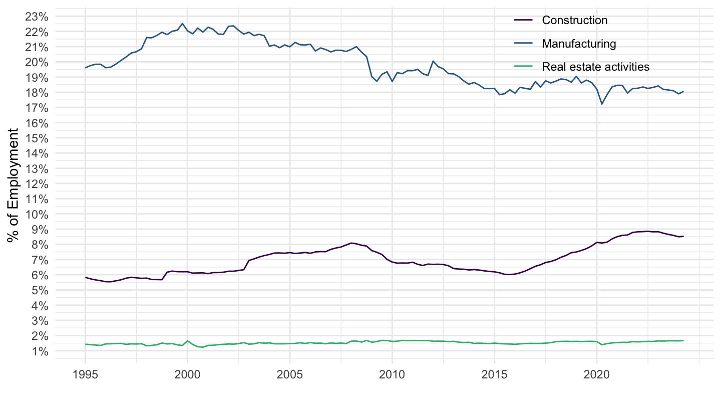
Portugal
Code
namq_10_a10_e %>%
  filter(na_item == "EMP_DC",
         nace_r2 %in% c("C", "TOTAL", "L", "F"),
         geo %in% c("PT"),
         s_adj == "SCA",
         unit== "THS_HW") %>%
  quarter_to_date() %>%
  left_join(nace_r2, by = "nace_r2") %>%
  select(nace_r2, Nace_r2, date, values) %>%
  group_by(date) %>%
  mutate(values = values/ values[nace_r2 == "TOTAL"]) %>%
  filter(nace_r2 != "TOTAL")  %>%
  ggplot(.) + geom_line(aes(x = date, y = values, color = Nace_r2)) +
  theme_minimal() + xlab("") + ylab("% of Employment") +
  scale_color_manual(values = viridis(4)[1:3]) +
  scale_x_date(breaks = seq(1960, 2100, 5) %>% paste0("-01-01") %>% as.Date,
               labels = date_format("%Y")) +
  scale_y_continuous(breaks = 0.01*seq(-500, 200, 1),
                     labels = percent_format(accuracy = 1)) +
  theme(legend.position = c(0.8, 0.9),
        legend.title = element_blank())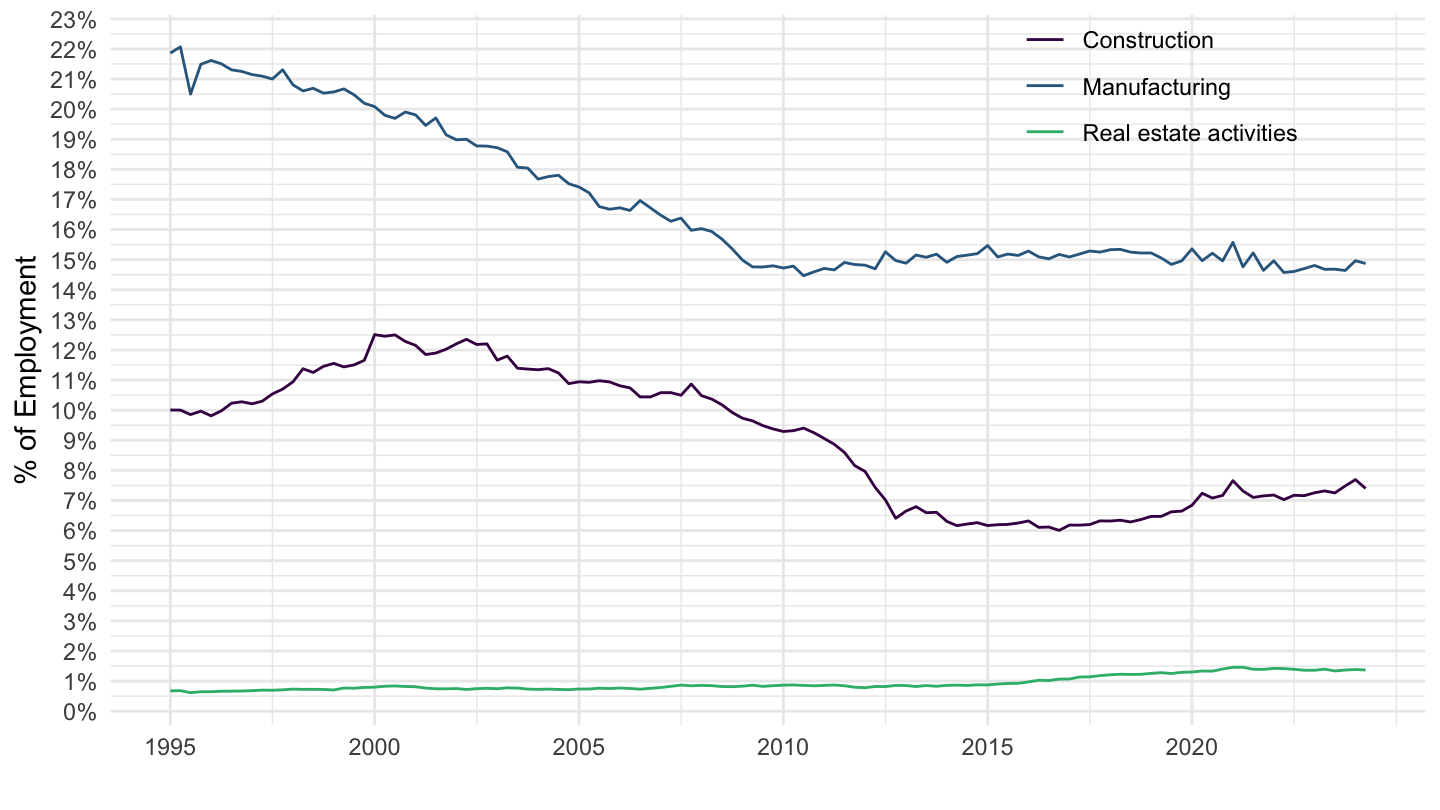
Austria
Code
namq_10_a10_e %>%
  filter(na_item == "EMP_DC",
         nace_r2 %in% c("C", "TOTAL", "L", "F"),
         geo %in% c("AT"),
         s_adj == "SCA",
         unit== "THS_HW") %>%
  quarter_to_date() %>%
  left_join(nace_r2, by = "nace_r2") %>%
  select(nace_r2, Nace_r2, date, values) %>%
  group_by(date) %>%
  mutate(values = values/ values[nace_r2 == "TOTAL"]) %>%
  filter(nace_r2 != "TOTAL")  %>%
  ggplot(.) + geom_line(aes(x = date, y = values, color = Nace_r2)) +
  theme_minimal() + xlab("") + ylab("% of Employment") +
  scale_color_manual(values = viridis(4)[1:3]) +
  scale_x_date(breaks = seq(1960, 2100, 5) %>% paste0("-01-01") %>% as.Date,
               labels = date_format("%Y")) +
  scale_y_continuous(breaks = 0.01*seq(-500, 200, 1),
                     labels = percent_format(accuracy = 1)) +
  theme(legend.position = c(0.8, 0.9),
        legend.title = element_blank())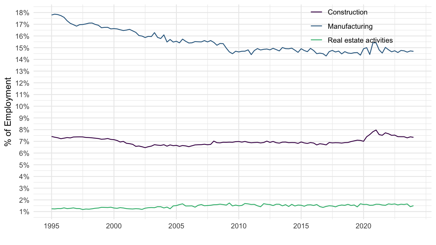
Sweden
Code
namq_10_a10_e %>%
  filter(na_item == "EMP_DC",
         nace_r2 %in% c("C", "TOTAL", "L", "F"),
         geo %in% c("SE"),
         s_adj == "SCA",
         unit== "THS_HW") %>%
  quarter_to_date() %>%
  left_join(nace_r2, by = "nace_r2") %>%
  select(nace_r2, Nace_r2, date, values) %>%
  group_by(date) %>%
  mutate(values = values/ values[nace_r2 == "TOTAL"]) %>%
  filter(nace_r2 != "TOTAL")  %>%
  ggplot(.) + geom_line(aes(x = date, y = values, color = Nace_r2)) +
  theme_minimal() + xlab("") + ylab("% of Employment") +
  scale_color_manual(values = viridis(4)[1:3]) +
  scale_x_date(breaks = seq(1960, 2100, 5) %>% paste0("-01-01") %>% as.Date,
               labels = date_format("%Y")) +
  scale_y_continuous(breaks = 0.01*seq(-500, 200, 1),
                     labels = percent_format(accuracy = 1)) +
  theme(legend.position = c(0.8, 0.9),
        legend.title = element_blank())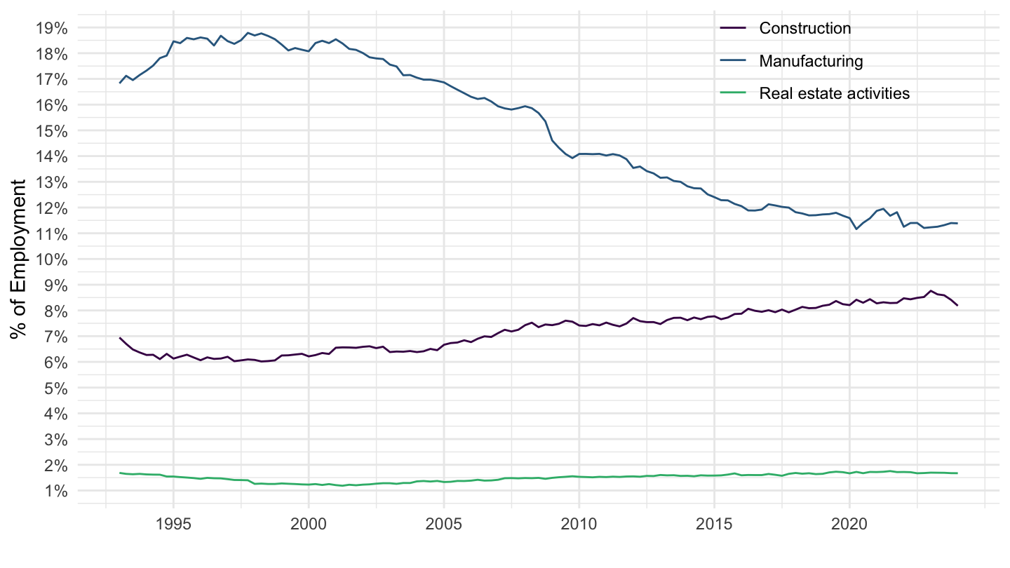
United Kingdom
Code
namq_10_a10_e %>%
  filter(na_item == "EMP_DC",
         nace_r2 %in% c("C", "TOTAL", "L", "F"),
         geo %in% c("UK"),
         s_adj == "SCA",
         unit== "THS_HW") %>%
  quarter_to_date() %>%
  left_join(nace_r2, by = "nace_r2") %>%
  select(nace_r2, Nace_r2, date, values) %>%
  group_by(date) %>%
  mutate(values = values/ values[nace_r2 == "TOTAL"]) %>%
  filter(nace_r2 != "TOTAL")  %>%
  ggplot(.) + geom_line(aes(x = date, y = values, color = Nace_r2)) +
  theme_minimal() + xlab("") + ylab("% of Employment") +
  scale_color_manual(values = viridis(4)[1:3]) +
  scale_x_date(breaks = seq(1960, 2100, 5) %>% paste0("-01-01") %>% as.Date,
               labels = date_format("%Y")) +
  scale_y_continuous(breaks = 0.01*seq(-500, 200, 1),
                     labels = percent_format(accuracy = 1)) +
  theme(legend.position = c(0.8, 0.9),
        legend.title = element_blank())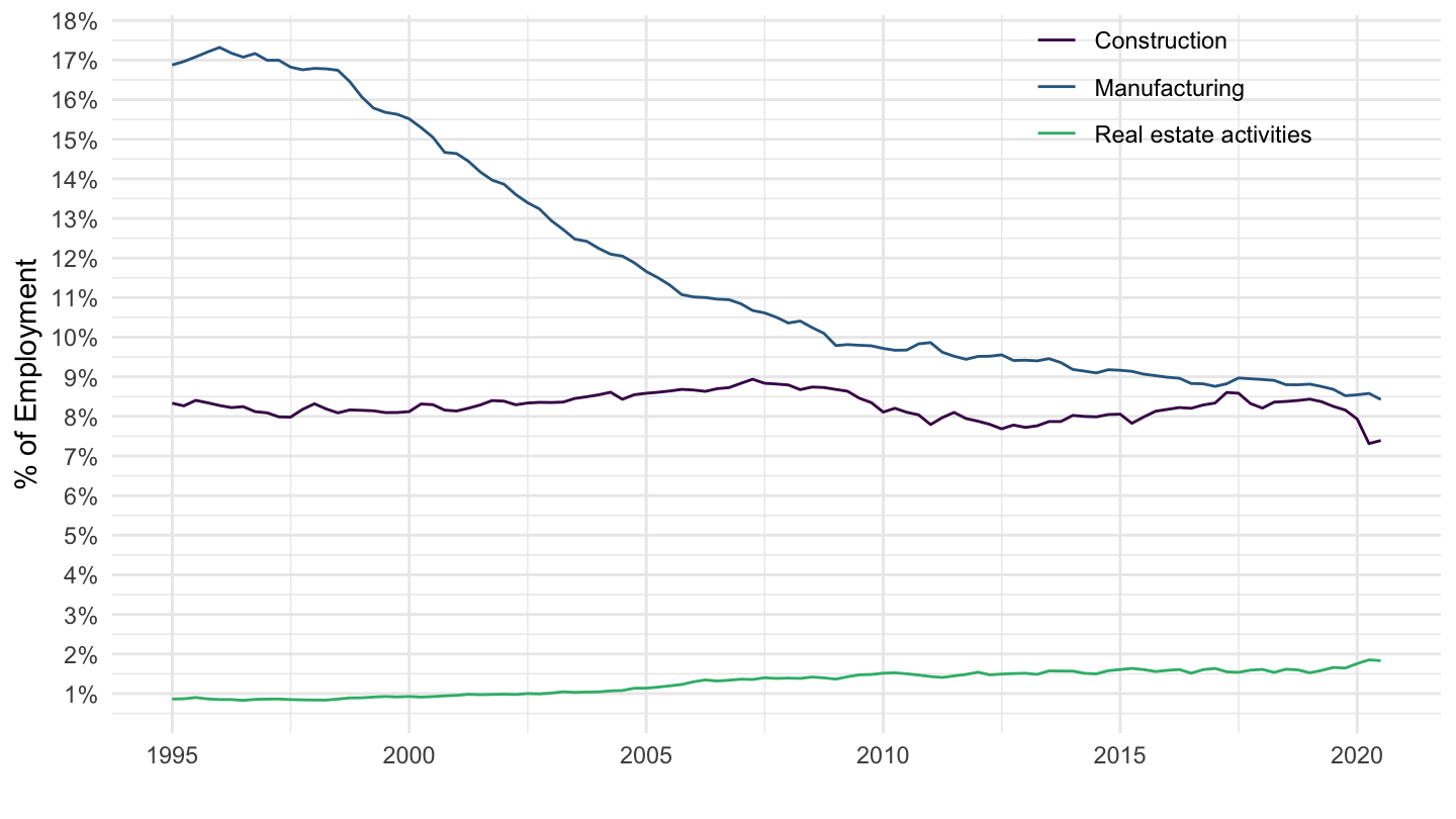
France, Germany, Italy
Number of hours worked
All
Code
namq_10_a10_e %>%
  left_join(geo, by = "geo") %>%
  filter(geo %in% c("FR", "DE", "IT"),
         nace_r2 == "C",
         s_adj == "SCA",
         unit == "THS_HW",
         na_item == "EMP_DC") %>%
  quarter_to_date() %>%
  arrange(date) %>%
  mutate(values = values/1000) %>%
  left_join(colors, by = c("Geo" = "country")) %>%
  ggplot(.) + geom_line(aes(x = date, y = values, color = color)) +
  theme_minimal() + xlab("") + ylab("Number of Hours Worked, Millions") +
  scale_x_date(breaks = seq(1960, 2100, 5) %>% paste0("-01-01") %>% as.Date,
               labels = date_format("%Y")) +
  scale_y_continuous(breaks = seq(0, 1000000, 500),
                     labels = dollar_format(accuracy = 1, prefix = "", suffix = "M")) +
  scale_color_identity() + add_3flags +
  theme(legend.position = c(0.2, 0.80),
        legend.title = element_blank())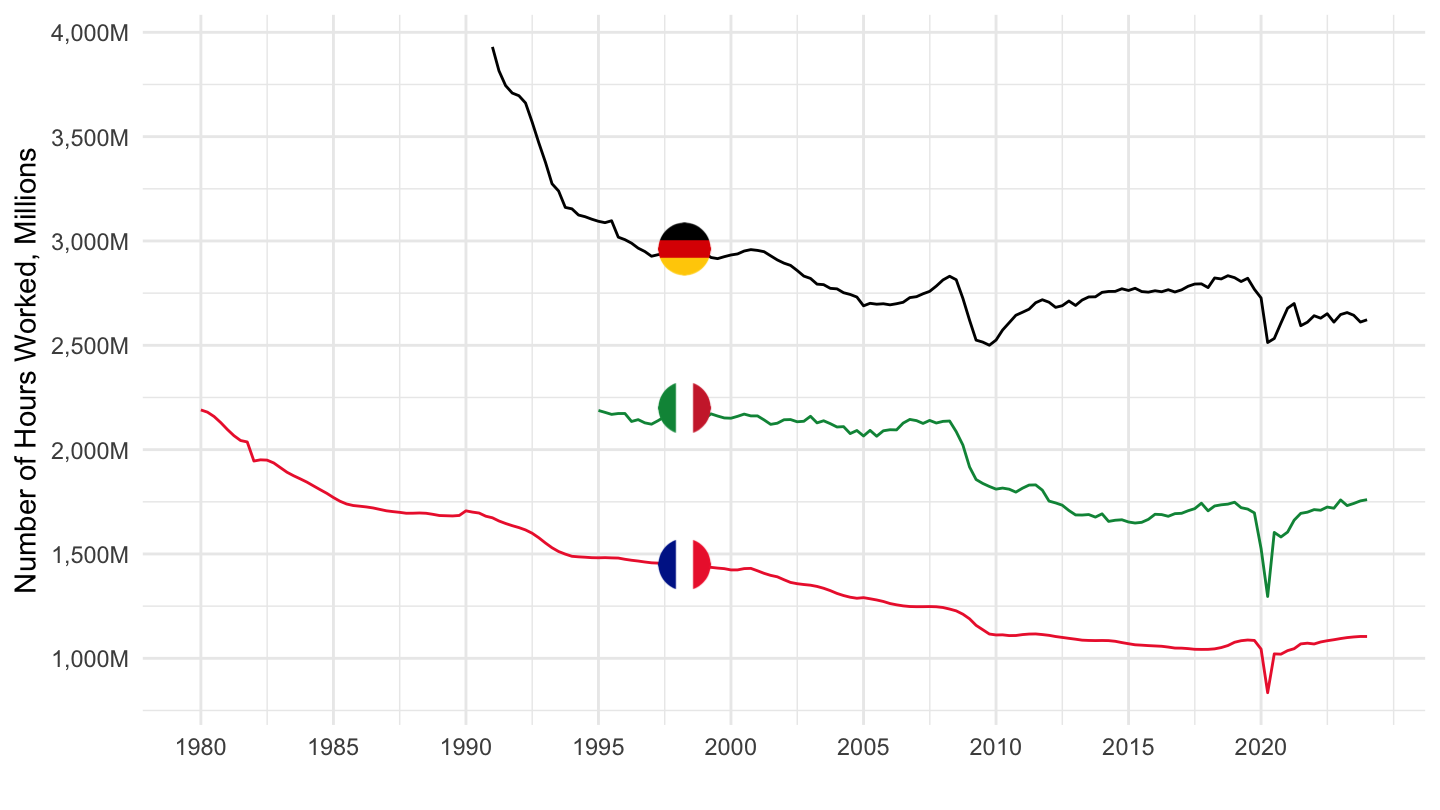
2000-
Code
namq_10_a10_e %>%
  left_join(geo, by = "geo") %>%
  filter(geo %in% c("FR", "DE", "IT"),
         nace_r2 == "C",
         s_adj == "SCA",
         unit == "THS_HW",
         na_item == "EMP_DC") %>%
  quarter_to_date() %>%
  filter(date >= as.Date("2000-01-01")) %>%
  arrange(date) %>%
  mutate(values = values/1000) %>%
  left_join(colors, by = c("Geo" = "country")) %>%
  ggplot(.) + geom_line(aes(x = date, y = values, color = color)) +
  theme_minimal() + xlab("") + ylab("Number of Hours Worked, Millions") +
  scale_x_date(breaks = seq(1960, 2100, 5) %>% paste0("-01-01") %>% as.Date,
               labels = date_format("%Y")) +
  scale_y_continuous(breaks = seq(0, 1000000, 500),
                     labels = dollar_format(accuracy = 1, prefix = "", suffix = "M")) +
  scale_color_identity() + add_3flags +
  theme(legend.position = c(0.2, 0.80),
        legend.title = element_blank())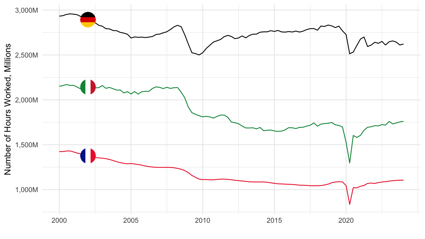
Number of employees
France, Germany, Italy
All
All
Code
namq_10_a10_e %>%
  left_join(geo, by = "geo") %>%
  filter(geo %in% c("FR", "DE", "IT"),
         nace_r2 == "C",
         s_adj == "NSA",
         unit == "THS_PER",
         na_item == "EMP_DC") %>%
  quarter_to_date() %>%
  arrange(date) %>%
  left_join(colors, by = c("Geo" = "country")) %>%
  ggplot(.) + geom_line(aes(x = date, y = values, color = color)) +
  theme_minimal() + xlab("") + ylab("Number of Employees, '000") +
  scale_x_date(breaks = seq(1960, 2100, 5) %>% paste0("-01-01") %>% as.Date,
               labels = date_format("%Y")) +
  scale_y_continuous(breaks = seq(0, 1000000, 1000),
                     labels = dollar_format(accuracy = 1, prefix = "", suffix = "M")) +
  scale_color_identity() + add_3flags +
  theme(legend.position = c(0.2, 0.80),
        legend.title = element_blank())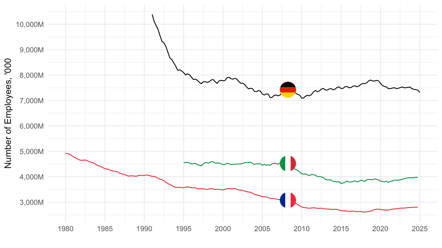
1995-
Code
namq_10_a10_e %>%
  left_join(geo, by = "geo") %>%
  filter(geo %in% c("FR", "DE", "IT"),
         nace_r2 == "C",
         s_adj == "NSA",
         unit == "THS_PER",
         na_item == "EMP_DC") %>%
  quarter_to_date() %>%
  arrange(date) %>%
  filter(date >= as.Date("1995-01-01")) %>%
  left_join(colors, by = c("Geo" = "country")) %>%
  ggplot(.) + geom_line(aes(x = date, y = values, color = color)) +
  theme_minimal() + xlab("") + ylab("Number of Employees, '000") +
  scale_x_date(breaks = seq(1960, 2100, 5) %>% paste0("-01-01") %>% as.Date,
               labels = date_format("%Y")) +
  scale_y_continuous(breaks = seq(0, 1000000, 1000),
                     labels = dollar_format(accuracy = 1, prefix = "", suffix = "M")) +
  scale_color_identity() + add_3flags +
  theme(legend.position = c(0.2, 0.80),
        legend.title = element_blank())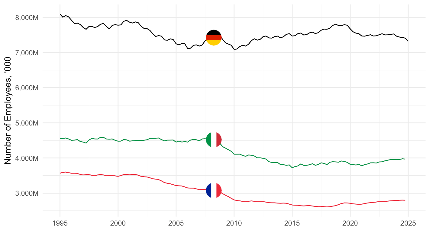
All
All
Code
namq_10_a10_e %>%
  left_join(geo, by = "geo") %>%
  filter(geo %in% c("FR", "DE", "IT"),
         nace_r2 == "TOTAL",
         s_adj == "NSA",
         unit == "THS_PER",
         na_item == "EMP_DC") %>%
  quarter_to_date() %>%
  arrange(date) %>%
  left_join(colors, by = c("Geo" = "country")) %>%
  ggplot(.) + geom_line(aes(x = date, y = values, color = color)) +
  theme_minimal() + xlab("") + ylab("Number of Employees, '000") +
  scale_x_date(breaks = seq(1960, 2100, 5) %>% paste0("-01-01") %>% as.Date,
               labels = date_format("%Y")) +
  scale_y_continuous(breaks = seq(0, 1000000, 5000),
                     labels = dollar_format(accuracy = 1, prefix = "", suffix = "M")) +
  scale_color_identity() + add_3flags +
  theme(legend.position = c(0.2, 0.80),
        legend.title = element_blank())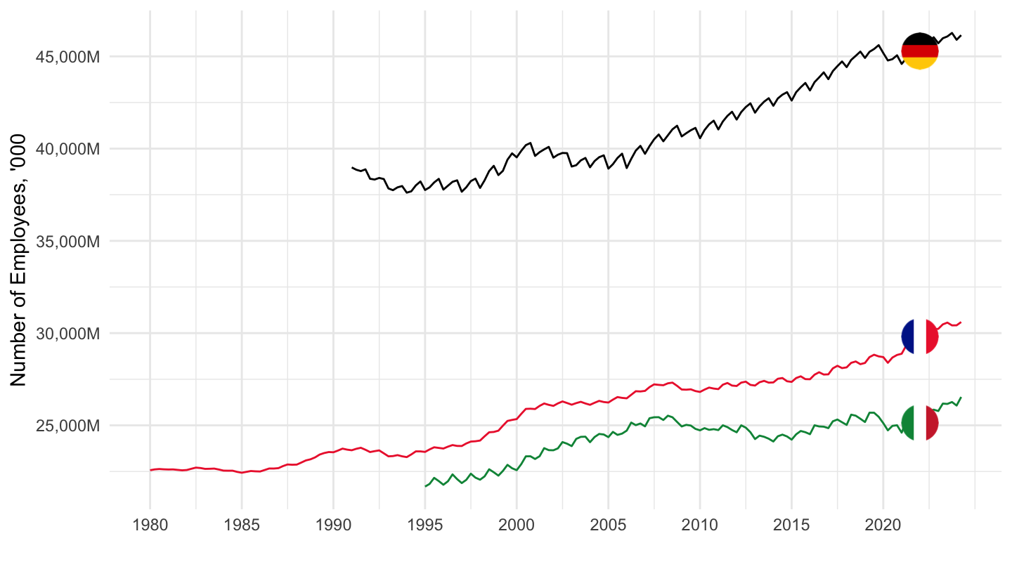
2000-
Code
namq_10_a10_e %>%
  left_join(geo, by = "geo") %>%
  filter(geo %in% c("FR", "DE", "IT"),
         nace_r2 == "TOTAL",
         s_adj == "NSA",
         unit == "THS_PER",
         na_item == "EMP_DC") %>%
  quarter_to_date() %>%
  filter(date >= as.Date("2000-01-01")) %>%
  arrange(date) %>%
  left_join(colors, by = c("Geo" = "country")) %>%
  ggplot(.) + geom_line(aes(x = date, y = values, color = color)) +
  theme_minimal() + xlab("") + ylab("Number of Employees, '000") +
  scale_x_date(breaks = seq(1960, 2100, 5) %>% paste0("-01-01") %>% as.Date,
               labels = date_format("%Y")) +
  scale_y_continuous(breaks = seq(0, 1000000, 5000),
                     labels = dollar_format(accuracy = 1, prefix = "", suffix = "M")) +
  scale_color_identity() + add_3flags +
  theme(legend.position = c(0.2, 0.80),
        legend.title = element_blank())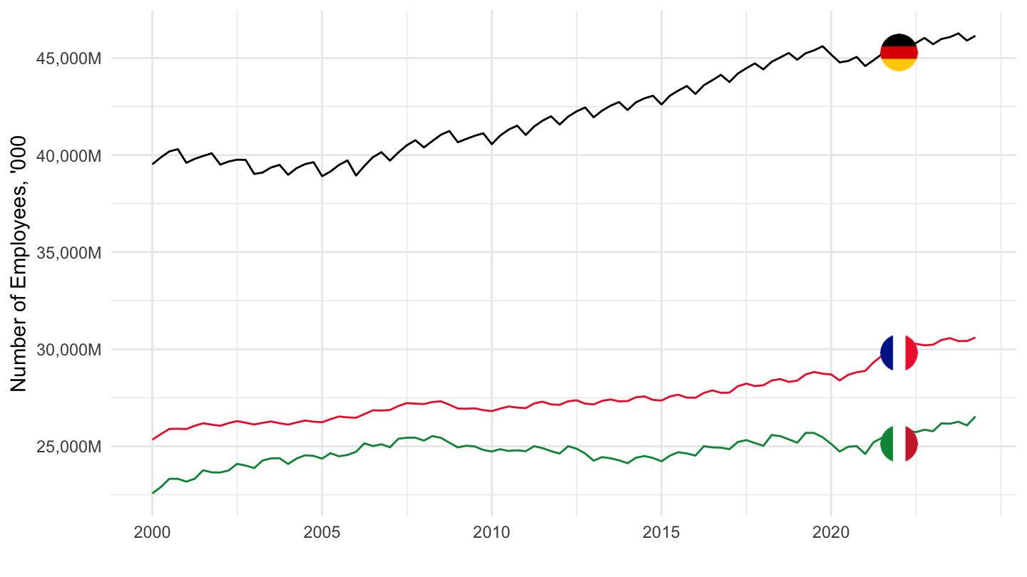
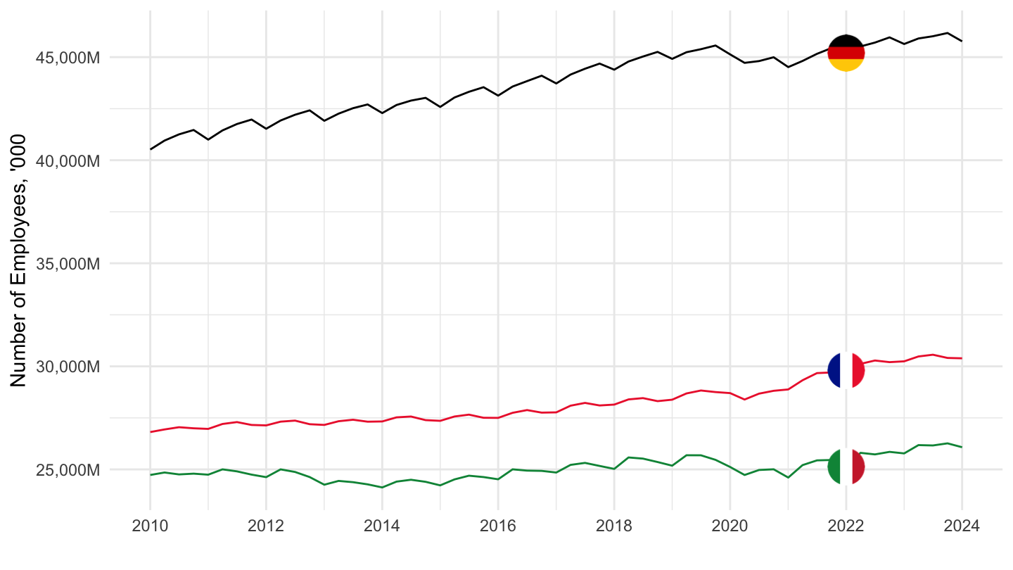
2010-
Code
namq_10_a10_e %>%
  left_join(geo, by = "geo") %>%
  filter(geo %in% c("FR", "DE", "IT"),
         nace_r2 == "TOTAL",
         s_adj == "NSA",
         unit == "THS_PER",
         na_item == "EMP_DC") %>%
  quarter_to_date() %>%
  filter(date >= as.Date("2010-01-01")) %>%
  arrange(date) %>%
  left_join(colors, by = c("Geo" = "country")) %>%
  ggplot(.) + geom_line(aes(x = date, y = values, color = color)) +
  theme_minimal() + xlab("") + ylab("Number of Employees, '000") +
  scale_x_date(breaks = seq(1960, 2026, 2) %>% paste0("-01-01") %>% as.Date,
               labels = date_format("%Y")) +
  scale_y_continuous(breaks = seq(0, 1000000, 5000),
                     labels = dollar_format(accuracy = 1, prefix = "", suffix = "M")) +
  scale_color_identity() + add_3flags +
  theme(legend.position = c(0.2, 0.80),
        legend.title = element_blank())