Gross value added and income A*10 industry breakdowns
Data - Eurostat
Info
Last observation: Quarterly: 2026Q1 (N = 45,456)
First observation: Quarterly: 1978Q1 (N = 576)
Last data update: 24 jul 2026, 18:34. Last compile: 25 jul 2026, 20:22
Structure
Tables
B-E, C, TOTAL
Code
namq_10_a10 %>%
  filter(nace_r2 %in% c("C", "TOTAL"),
         na_item == "B1G",
         # SCA: Seasonally and calendar adjusted data
         s_adj == "SCA",
         # CLV10_MEUR: Chain linked volumes (2010), million euro
         unit == "CP_MNAC",
         time %in% c("2021Q4", "2016Q4", "2011Q4")) %>%


  select(nace_r2, geo, Geo, values, time) %>%
  spread(nace_r2, values) %>%
  mutate(C_TOTAL = 100*C/TOTAL) %>%
  select(-C, -TOTAL) %>%
  spread(time, C_TOTAL) %>%
  mutate(Geo = ifelse(geo == "DE", "Germany", Geo)) %>%
  mutate(Flag = gsub(" ", "-", str_to_lower(Geo)),
         Flag = paste0('<img src="../../bib/flags/vsmall/', Flag, '.png" alt="Flag">')) %>%
  select(Flag, everything()) %>%
  arrange(`2021Q4`) %>%
  {if (is_html_output()) datatable(., filter = 'top', rownames = F, escape = F) else .}
B-E, TOTAL
Code
namq_10_a10 %>%
  filter(nace_r2 %in% c("B-E", "TOTAL"),
         na_item == "B1G",
         # SCA: Seasonally and calendar adjusted data
         s_adj == "SCA",
         # CLV10_MEUR: Chain linked volumes (2010), million euro
         unit == "CP_MNAC",
         time %in% c("2021Q4", "2001Q4", "2011Q4")) %>%


  select(nace_r2, geo, Geo, values, time) %>%
  spread(nace_r2, values) %>%
  mutate(C_TOTAL = 100*`B-E`/TOTAL) %>%
  select(-`B-E`, -TOTAL) %>%
  spread(time, C_TOTAL) %>%
  mutate(Geo = ifelse(geo == "DE", "Germany", Geo)) %>%
  mutate(Flag = gsub(" ", "-", str_to_lower(Geo)),
         Flag = paste0('<img src="../../bib/flags/vsmall/', Flag, '.png" alt="Flag">')) %>%
  select(Flag, everything()) %>%
  arrange(`2021Q4`) %>%
  {if (is_html_output()) datatable(., filter = 'top', rownames = F, escape = F) else .}
B-E, C, TOTAL
Code
load_data("eurostat/geo_fr.RData")
geo_fr <- geo
load_data("eurostat/geo.RData")
namq_10_a10 %>%
  filter(nace_r2 %in% c("B-E", "TOTAL", "C"),
         na_item == "B1G",
         # SCA: Seasonally and calendar adjusted data
         s_adj == "SCA",
         # CLV10_MEUR: Chain linked volumes (2010), million euro
         unit == "CP_MNAC",
         time %in% c("2021Q4")) %>%

  select(nace_r2, geo, Geo, values) %>%
  spread(nace_r2, values) %>%
  mutate(`Industrie Manufacturière` = round(100*`C`/TOTAL, 1),
         `Industrie Manufacturière + Energie` = round(100*`B-E`/TOTAL, 1)) %>%
  select(-`B-E`, -TOTAL, -`C`) %>%
  mutate(Geo = ifelse(geo == "DE", "Germany", Geo)) %>%
  mutate(Flag = gsub(" ", "-", str_to_lower(Geo)),
         Flag = paste0('<img src="../../bib/flags/vsmall/', Flag, '.png" alt="Flag">')) %>%
  select(Flag, everything()) %>%
  select(-Geo) %>%
  left_join(geo_fr, by = "geo") %>%
  select(-geo) %>%
  select(Flag, Geo, everything()) %>%
  arrange(`Industrie Manufacturière + Energie`) %>%
  {if (is_html_output()) datatable(., filter = 'top', rownames = F, escape = F) else .}
PD20_EUR - Price index (implicit deflator), 2020=100, euro
C
1995-
Code
namq_10_a10 %>%
  filter(geo %in% c("FR", "DE", "IT", "ES", "EA21"),
         nace_r2 == "C",
         s_adj == "SCA",
         unit == "PD20_EUR") %>%
  quarter_to_date %>%
  filter(date >= as.Date("1995-01-01")) %>%

  mutate(Geo = ifelse(geo == "EA21", "Europe", Geo)) %>%
  left_join(colors, by = c("Geo" = "country")) %>%
  mutate(values = values/100) %>%
  group_by(Geo) %>%
  arrange(date) %>%
  mutate(values = 100*values/values[1]) %>%
  ggplot + geom_line(aes(x = date, y = values, color = color)) +
  scale_color_identity() + theme_minimal() + xlab("") + ylab("C - Manufacturing \n PD20_EUR - Price index (implicit deflator), 1995T1=100") + add_flags +
  scale_x_date(breaks = as.Date(paste0(seq(1960, 2100, 5), "-01-01")),
               labels = date_format("%Y")) + add_flags +
  scale_y_continuous(breaks = seq(10, 300, 10)) +
  theme(legend.position = c(0.35, 0.85),
        legend.title = element_blank()) +
  geom_label(data = . %>% filter(date == max(date)), aes(x = date, y = values, label = round(values), color = color))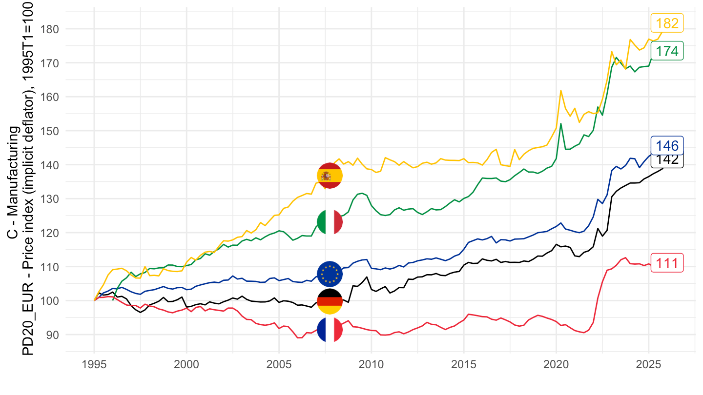
1995-
Code
namq_10_a10 %>%
  filter(nace_r2 == "C",
         s_adj == "SCA",
         unit == "PD20_EUR") %>%
  quarter_to_date %>%
  filter(date >= as.Date("1995-01-01")) %>%

  mutate(Geo = ifelse(geo == "EA21", "Europe", Geo)) %>%
  left_join(colors, by = c("Geo" = "country")) %>%
  mutate(values = values/100) %>%
  group_by(Geo) %>%
  arrange(date) %>%
  mutate(values = 100*values/values[1]) %>%
  ggplot + geom_line(aes(x = date, y = values, color = Geo)) +
  theme_minimal() + xlab("") + ylab("") + add_flags +
  scale_x_date(breaks = as.Date(paste0(seq(1960, 2100, 5), "-01-01")),
               labels = date_format("%Y")) + add_flags +
  scale_y_continuous(breaks = seq(10, 300, 10),
                     limits = c(90, 130)) +
  theme(legend.position = c(0.35, 0.85),
        legend.title = element_blank())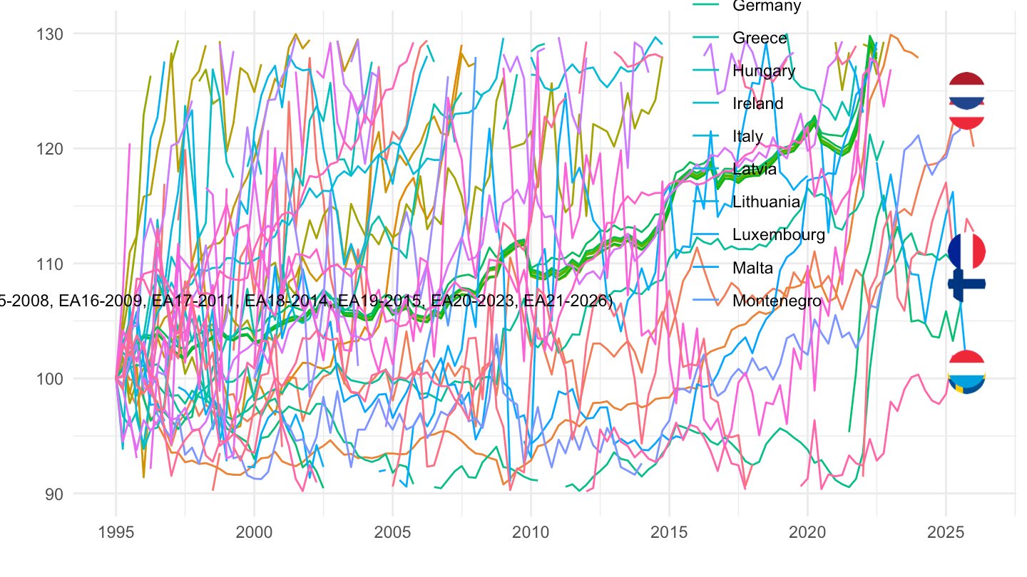
PD_PCH_SM_EUR - Price index
France, Germany, Italy
TOTAL
1995-
Code
namq_10_a10 %>%
  filter(geo %in% c("FR", "DE", "IT"),
         nace_r2 == "TOTAL",
         s_adj == "SCA",
         unit == "PD_PCH_SM_EUR") %>%
  quarter_to_date %>%
  filter(date >= as.Date("1995-01-01")) %>%

  left_join(colors, by = c("Geo" = "country")) %>%
  mutate(values = values/100) %>%
  ggplot + geom_line(aes(x = date, y = values, color = color)) +
  scale_color_identity() + theme_minimal() + xlab("") + ylab("") + add_flags +
  scale_x_date(breaks = as.Date(paste0(seq(1960, 2100, 5), "-01-01")),
               labels = date_format("%Y")) +
  theme(legend.position = c(0.35, 0.85),
        legend.title = element_blank()) +
  scale_y_continuous(breaks = 0.01*seq(-10, 1000, 1),
                     labels = percent_format(accuracy = 1))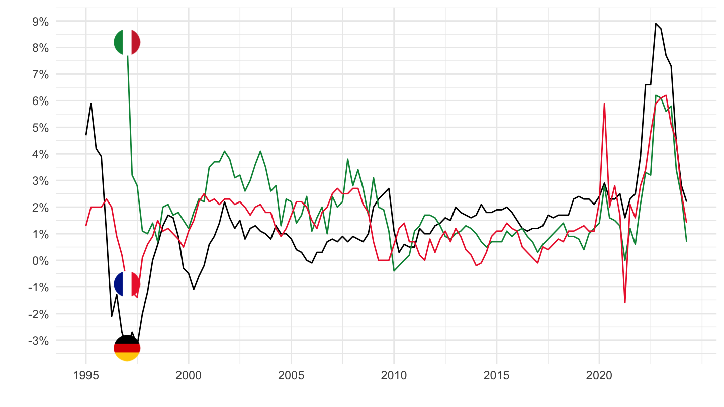
2015-
Code
namq_10_a10 %>%
  filter(geo %in% c("FR", "DE", "IT"),
         nace_r2 == "TOTAL",
         s_adj == "SCA",
         unit == "PD_PCH_SM_EUR") %>%
  quarter_to_date %>%
  filter(date >= as.Date("2015-01-01")) %>%

  left_join(colors, by = c("Geo" = "country")) %>%
  mutate(values = values/100) %>%
  ggplot + geom_line(aes(x = date, y = values, color = color)) +
  scale_color_identity() + theme_minimal() + xlab("") + ylab("") + add_flags +
  scale_x_date(breaks = as.Date(paste0(seq(1960, 2100, 1), "-01-01")),
               labels = date_format("%Y")) +
  theme(legend.position = c(0.35, 0.85),
        legend.title = element_blank()) +
  scale_y_continuous(breaks = 0.01*seq(-10, 1000, 1),
                     labels = percent_format(accuracy = 1))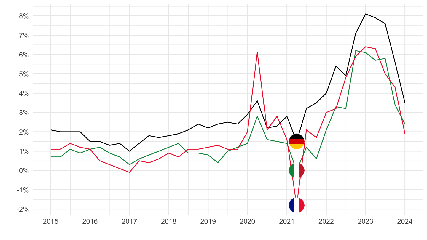
A
1995-
Code
namq_10_a10 %>%
  filter(geo %in% c("FR", "DE", "IT"),
         nace_r2 == "A",
         s_adj == "SCA",
         unit == "PD_PCH_SM_EUR") %>%
  quarter_to_date %>%
  filter(date >= as.Date("1995-01-01")) %>%

  left_join(colors, by = c("Geo" = "country")) %>%
  mutate(values = values/100) %>%
  ggplot + geom_line(aes(x = date, y = values, color = color)) +
  scale_color_identity() + theme_minimal() + xlab("") + ylab("") + add_flags +
  scale_x_date(breaks = as.Date(paste0(seq(1960, 2100, 5), "-01-01")),
               labels = date_format("%Y")) +
  theme(legend.position = c(0.35, 0.85),
        legend.title = element_blank()) +
  scale_y_continuous(breaks = 0.01*seq(-100, 1000, 10),
                     labels = percent_format(accuracy = 1))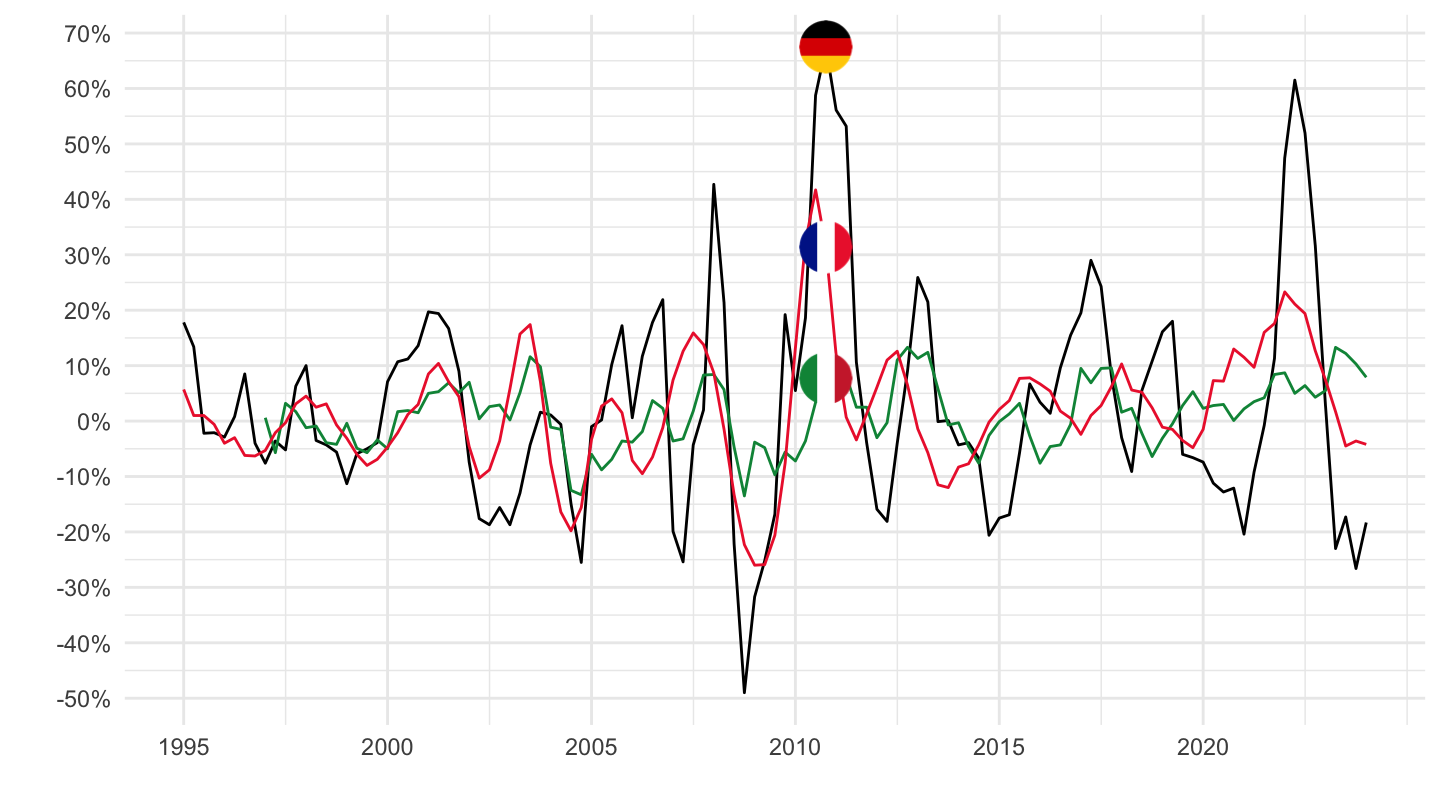
2015-
Code
namq_10_a10 %>%
  filter(geo %in% c("FR", "DE", "IT"),
         nace_r2 == "A",
         s_adj == "SCA",
         unit == "PD_PCH_SM_EUR") %>%
  quarter_to_date %>%
  filter(date >= as.Date("2015-01-01")) %>%

  left_join(colors, by = c("Geo" = "country")) %>%
  mutate(values = values/100) %>%
  ggplot + geom_line(aes(x = date, y = values, color = color)) +
  scale_color_identity() + theme_minimal() + xlab("") + ylab("") + add_flags +
  scale_x_date(breaks = as.Date(paste0(seq(1960, 2100, 1), "-01-01")),
               labels = date_format("%Y")) +
  theme(legend.position = c(0.35, 0.85),
        legend.title = element_blank()) +
  scale_y_continuous(breaks = 0.01*seq(-100, 1000, 5),
                     labels = percent_format(accuracy = 1))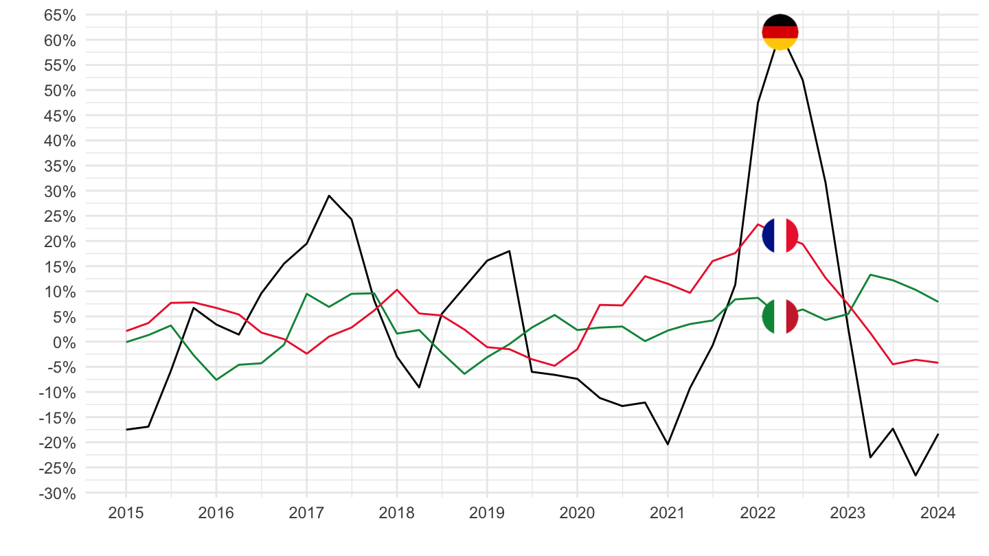
F
1995-
Code
namq_10_a10 %>%
  filter(geo %in% c("FR", "DE", "IT"),
         nace_r2 == "F",
         s_adj == "SCA",
         unit == "PD_PCH_SM_EUR") %>%
  quarter_to_date %>%
  filter(date >= as.Date("1995-01-01")) %>%

  left_join(colors, by = c("Geo" = "country")) %>%
  mutate(values = values/100) %>%
  ggplot + geom_line(aes(x = date, y = values, color = color)) +
  scale_color_identity() + theme_minimal() + xlab("") + ylab("") + add_flags +
  scale_x_date(breaks = as.Date(paste0(seq(1960, 2100, 5), "-01-01")),
               labels = date_format("%Y")) +
  theme(legend.position = c(0.35, 0.85),
        legend.title = element_blank()) +
  scale_y_continuous(breaks = 0.01*seq(-10, 1000, 1),
                     labels = percent_format(accuracy = 1))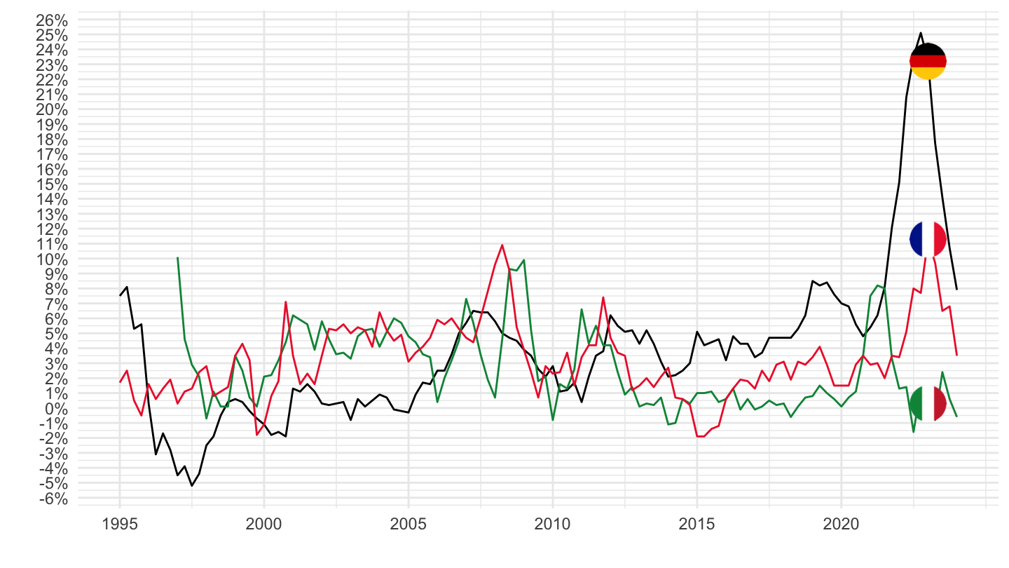
2015-
Code
namq_10_a10 %>%
  filter(geo %in% c("FR", "DE", "IT"),
         nace_r2 == "F",
         s_adj == "SCA",
         unit == "PD_PCH_SM_EUR") %>%
  quarter_to_date %>%
  filter(date >= as.Date("2015-01-01")) %>%

  left_join(colors, by = c("Geo" = "country")) %>%
  mutate(values = values/100) %>%
  ggplot + geom_line(aes(x = date, y = values, color = color)) +
  scale_color_identity() + theme_minimal() + xlab("") + ylab("") + add_flags +
  scale_x_date(breaks = as.Date(paste0(seq(1960, 2100, 1), "-01-01")),
               labels = date_format("%Y")) +
  theme(legend.position = c(0.35, 0.85),
        legend.title = element_blank()) +
  scale_y_continuous(breaks = 0.01*seq(-10, 1000, 1),
                     labels = percent_format(accuracy = 1))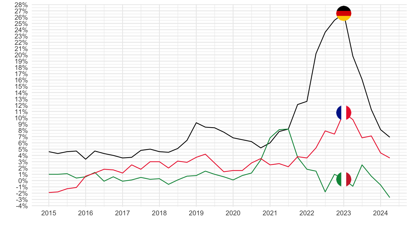
C
1995-
Code
namq_10_a10 %>%
  filter(geo %in% c("FR", "DE", "IT"),
         nace_r2 == "C",
         s_adj == "SCA",
         unit == "PD_PCH_SM_EUR") %>%
  quarter_to_date %>%
  filter(date >= as.Date("1995-01-01")) %>%

  left_join(colors, by = c("Geo" = "country")) %>%
  mutate(values = values/100) %>%
  ggplot + geom_line(aes(x = date, y = values, color = color)) +
  scale_color_identity() + theme_minimal() + xlab("") + ylab("") + add_flags +
  scale_x_date(breaks = as.Date(paste0(seq(1960, 2100, 5), "-01-01")),
               labels = date_format("%Y")) +
  theme(legend.position = c(0.35, 0.85),
        legend.title = element_blank()) +
  scale_y_continuous(breaks = 0.01*seq(-10, 1000, 1),
                     labels = percent_format(accuracy = 1))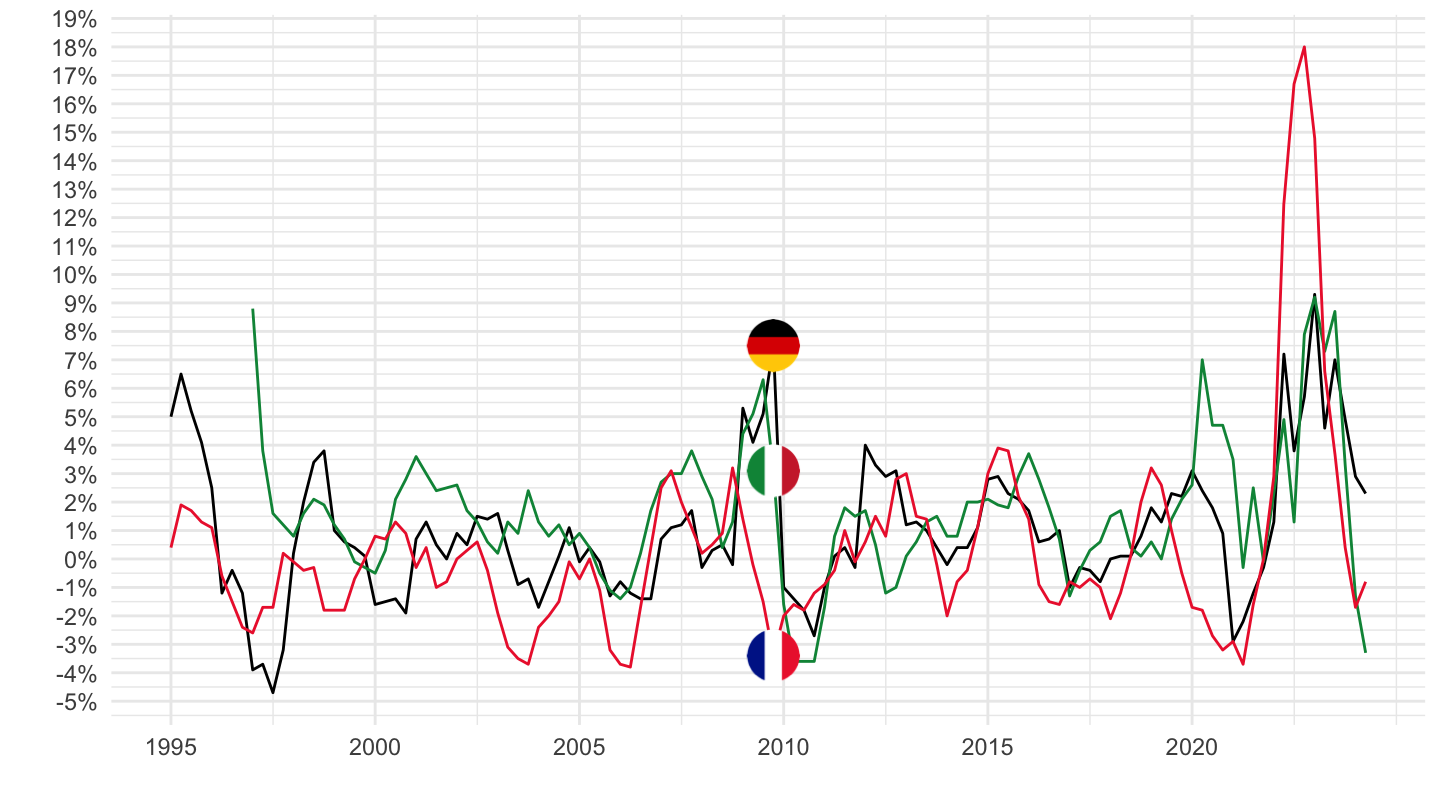
2015-
Code
namq_10_a10 %>%
  filter(geo %in% c("FR", "DE", "IT"),
         nace_r2 == "C",
         s_adj == "SCA",
         unit == "PD_PCH_SM_EUR") %>%
  quarter_to_date %>%
  filter(date >= as.Date("2015-01-01")) %>%

  left_join(colors, by = c("Geo" = "country")) %>%
  mutate(values = values/100) %>%
  ggplot + geom_line(aes(x = date, y = values, color = color)) +
  scale_color_identity() + theme_minimal() + xlab("") + ylab("") + add_flags +
  scale_x_date(breaks = as.Date(paste0(seq(1960, 2100, 1), "-01-01")),
               labels = date_format("%Y")) +
  theme(legend.position = c(0.35, 0.85),
        legend.title = element_blank()) +
  scale_y_continuous(breaks = 0.01*seq(-10, 1000, 1),
                     labels = percent_format(accuracy = 1))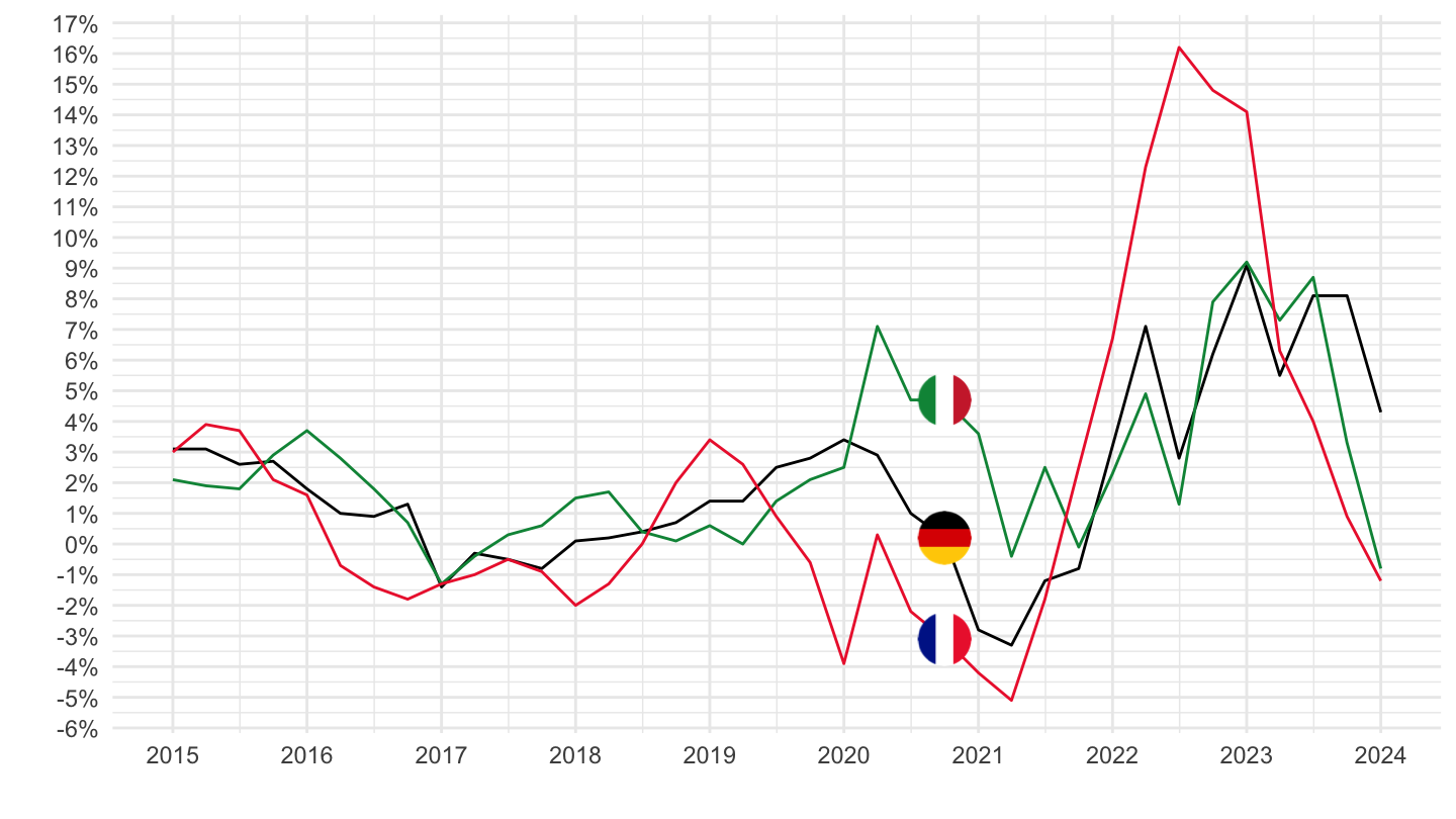
B-E
1995-
Code
namq_10_a10 %>%
  filter(geo %in% c("FR", "DE", "IT"),
         nace_r2 == "B-E",
         s_adj == "SCA",
         unit == "PD_PCH_SM_EUR") %>%
  quarter_to_date %>%
  filter(date >= as.Date("1995-01-01")) %>%

  left_join(colors, by = c("Geo" = "country")) %>%
  mutate(values = values/100) %>%
  ggplot + geom_line(aes(x = date, y = values, color = color)) +
  scale_color_identity() + theme_minimal() + xlab("") + ylab("") + add_flags +
  scale_x_date(breaks = as.Date(paste0(seq(1960, 2100, 5), "-01-01")),
               labels = date_format("%Y")) +
  theme(legend.position = c(0.35, 0.85),
        legend.title = element_blank()) +
  scale_y_continuous(breaks = 0.01*seq(-10, 1000, 1),
                     labels = percent_format(accuracy = 1))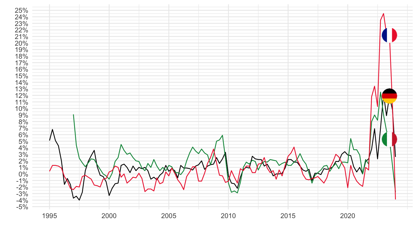
2015-
Code
namq_10_a10 %>%
  filter(geo %in% c("FR", "DE", "IT"),
         nace_r2 == "B-E",
         s_adj == "SCA",
         unit == "PD_PCH_SM_EUR") %>%
  quarter_to_date %>%
  filter(date >= as.Date("2015-01-01")) %>%

  left_join(colors, by = c("Geo" = "country")) %>%
  mutate(values = values/100) %>%
  ggplot + geom_line(aes(x = date, y = values, color = color)) +
  scale_color_identity() + theme_minimal() + xlab("") + ylab("") + add_flags +
  scale_x_date(breaks = as.Date(paste0(seq(1960, 2100, 1), "-01-01")),
               labels = date_format("%Y")) +
  theme(legend.position = c(0.35, 0.85),
        legend.title = element_blank()) +
  scale_y_continuous(breaks = 0.01*seq(-10, 1000, 1),
                     labels = percent_format(accuracy = 1))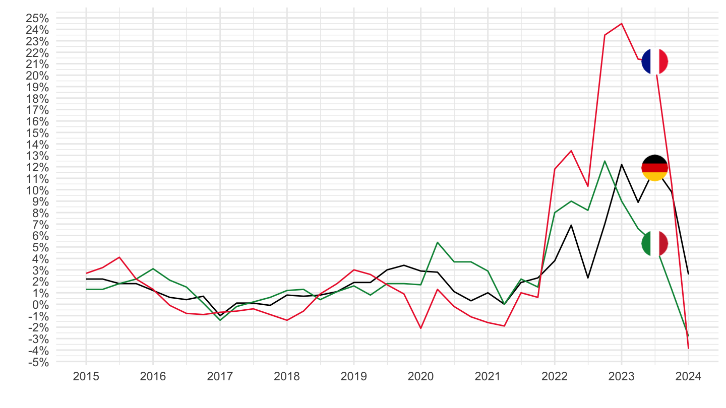
Manufacturing Value (Bn €)
Italy, France, Germany
Value
Code
namq_10_a10 %>%
  filter(geo %in% c("FR", "DE", "IT"),
         nace_r2 == "C",
         # B1GQ: Gross domestic product at market prices
         na_item == "B1G",
         # SCA: Seasonally and calendar adjusted data
         s_adj == "SCA",
         # CLV10_MEUR: Chain linked volumes (2010), million euro
         unit == "CP_MNAC") %>%
  quarter_to_date %>%
  filter(date >= as.Date("1995-01-01")) %>%

  left_join(colors, by = c("Geo" = "country")) %>%
  mutate(values = values/1000) %>%
  ggplot + geom_line(aes(x = date, y = values, color = color)) +
  scale_color_identity() + theme_minimal() + xlab("") + ylab("Production Manufacturière Trimestrielle") + add_flags +
  scale_x_date(breaks = as.Date(paste0(seq(1960, 2100, 5), "-01-01")),
               labels = date_format("%Y")) +
  theme(legend.position = c(0.35, 0.85),
        legend.title = element_blank()) +
  scale_y_log10(breaks = seq(0, 1000, 10),
                labels = dollar_format(suffix = " Mds€", prefix = "", accuracy = 1))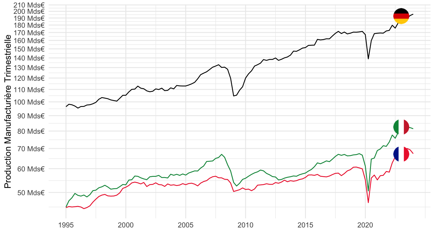
Manufacturing Value (Bn €)
Italy, France, Germany
Value
Code
namq_10_a10 %>%
  filter(geo %in% c("FR", "DE", "IT"),
         nace_r2 == "F",
         # B1GQ: Gross domestic product at market prices
         na_item == "B1G",
         # SCA: Seasonally and calendar adjusted data
         s_adj == "SCA",
         # CLV10_MEUR: Chain linked volumes (2010), million euro
         unit == "CP_MNAC") %>%
  quarter_to_date %>%
  filter(date >= as.Date("1995-01-01")) %>%

  left_join(colors, by = c("Geo" = "country")) %>%
  mutate(values = values/1000) %>%
  ggplot + geom_line(aes(x = date, y = values, color = color)) +
  scale_color_identity() + theme_minimal() + xlab("") + ylab("Construction en logements") + add_flags +
  scale_x_date(breaks = as.Date(paste0(seq(1960, 2100, 5), "-01-01")),
               labels = date_format("%Y")) +
  theme(legend.position = c(0.35, 0.85),
        legend.title = element_blank()) +
  scale_y_log10(breaks = seq(0, 1000, 10),
                labels = dollar_format(suffix = " Mds€", prefix = "", accuracy = 1))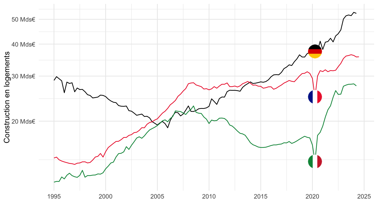
Volume
Code
namq_10_a10 %>%
  filter(geo %in% c("FR", "DE", "IT"),
         nace_r2 == "F",
         # B1GQ: Gross domestic product at market prices
         na_item == "B1G",
         # SCA: Seasonally and calendar adjusted data
         s_adj == "SCA",
         # CLV10_MEUR: Chain linked volumes (2010), million euro
         unit == "CLV15_MEUR") %>%
  quarter_to_date %>%
  filter(date >= as.Date("1995-01-01")) %>%

  left_join(colors, by = c("Geo" = "country")) %>%
  mutate(values = values/1000) %>%
  ggplot + geom_line(aes(x = date, y = values, color = color)) +
  scale_color_identity() + theme_minimal() + xlab("") + ylab("Construction en logements") + add_flags +
  scale_x_date(breaks = as.Date(paste0(seq(1960, 2100, 5), "-01-01")),
               labels = date_format("%Y")) +
  theme(legend.position = c(0.35, 0.85),
        legend.title = element_blank()) +
  scale_y_log10(breaks = seq(0, 1000, 10),
                labels = dollar_format(suffix = " Mds€", prefix = "", accuracy = 1))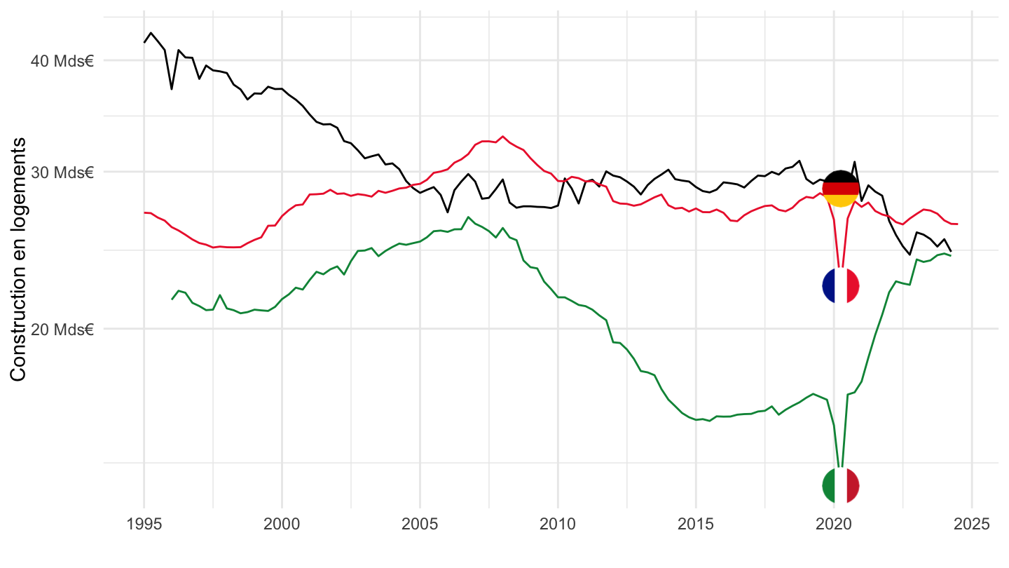
Indice
1990-
Code
namq_10_a10 %>%
  filter(geo %in% c("FR", "DE", "IT"),
         nace_r2 == "C",
         # B1GQ: Gross domestic product at market prices
         na_item == "B1G",
         # SCA: Seasonally and calendar adjusted data
         s_adj == "SCA",
         # CLV10_MEUR: Chain linked volumes (2010), million euro
         unit == "CP_MNAC") %>%
  quarter_to_date %>%
  filter(date >= as.Date("1990-01-01")) %>%

  left_join(colors, by = c("Geo" = "country")) %>%
  group_by(Geo) %>%
  arrange(date) %>%
  mutate(values = 100*values/values[1]) %>%
  ggplot + geom_line(aes(x = date, y = values, color = color)) +
  scale_color_identity() + theme_minimal() + xlab("") + ylab("Production Manufacturière Trimestrielle") + add_flags +
  scale_x_date(breaks = as.Date(paste0(seq(1960, 2100, 5), "-01-01")),
               labels = date_format("%Y")) +
  theme(legend.position = c(0.35, 0.85),
        legend.title = element_blank()) +
  scale_y_log10(breaks = seq(0, 1000, 5))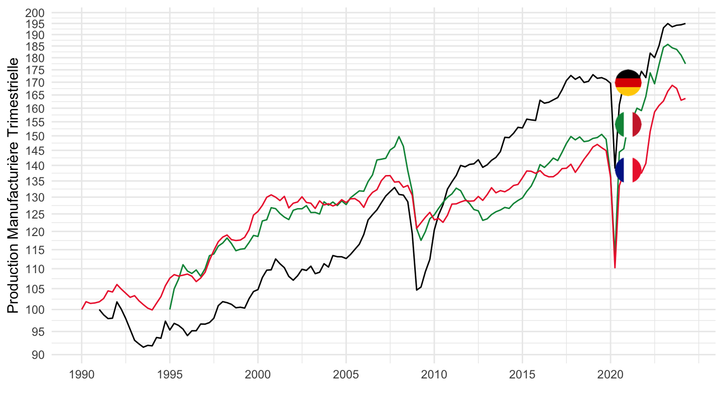
1995-
Code
namq_10_a10 %>%
  filter(geo %in% c("FR", "DE", "IT"),
         nace_r2 == "C",
         # B1GQ: Gross domestic product at market prices
         na_item == "B1G",
         # SCA: Seasonally and calendar adjusted data
         s_adj == "SCA",
         # CLV10_MEUR: Chain linked volumes (2010), million euro
         unit == "CP_MNAC") %>%
  quarter_to_date %>%
  filter(date >= as.Date("1995-01-01")) %>%

  left_join(colors, by = c("Geo" = "country")) %>%
  group_by(Geo) %>%
  arrange(date) %>%
  mutate(values = 100*values/values[1]) %>%
  ggplot + geom_line(aes(x = date, y = values, color = color)) +
  scale_color_identity() + theme_minimal() + xlab("") + ylab("Production Manufacturière Trimestrielle") + add_flags +
  scale_x_date(breaks = as.Date(paste0(seq(1960, 2100, 5), "-01-01")),
               labels = date_format("%Y")) +
  theme(legend.position = c(0.35, 0.85),
        legend.title = element_blank()) +
  scale_y_log10(breaks = seq(0, 1000, 5))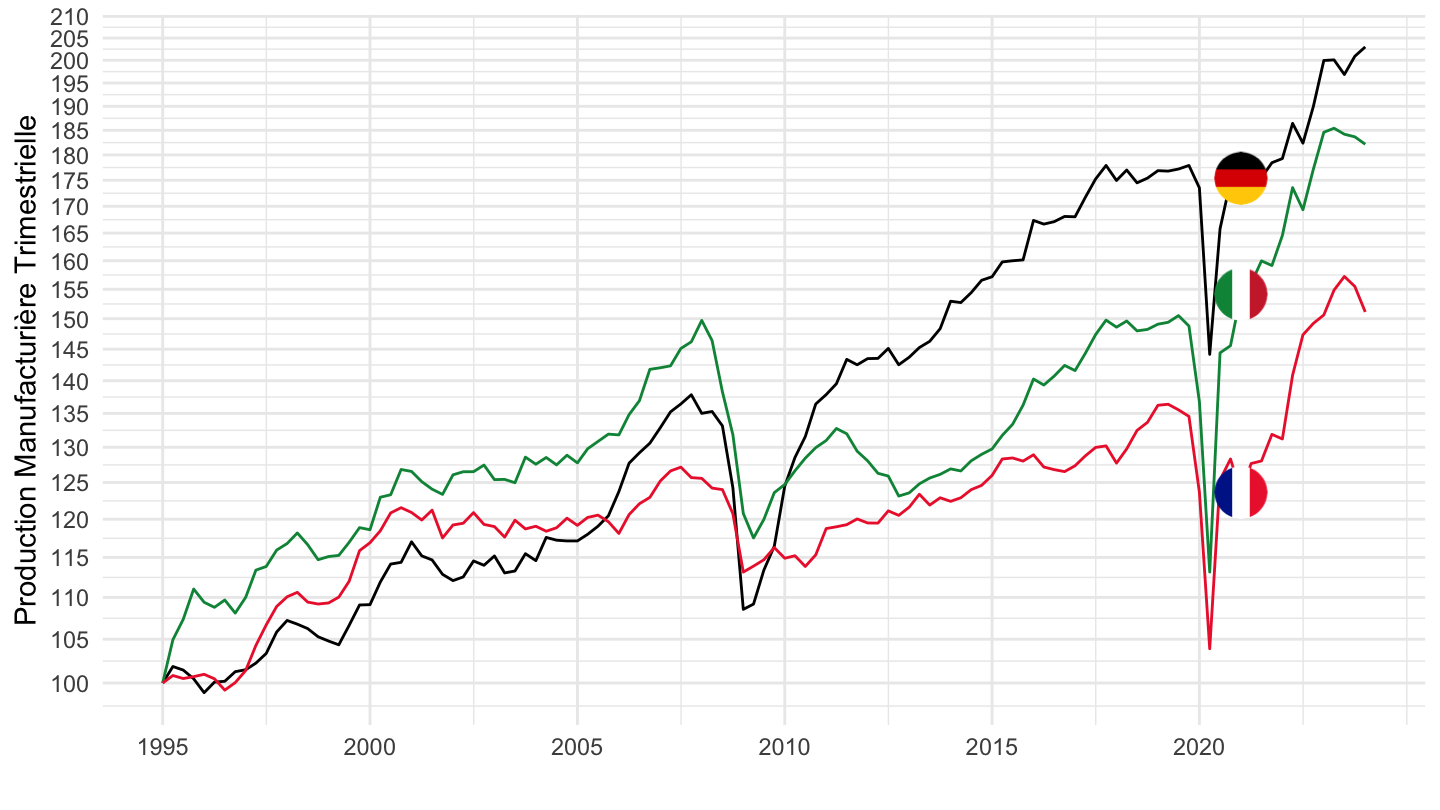
Code
namq_10_a10 %>%
  filter(geo %in% c("FR", "DE", "IT"),
         nace_r2 == "C",
         # B1GQ: Gross domestic product at market prices
         na_item == "B1G",
         # SCA: Seasonally and calendar adjusted data
         s_adj == "SCA",
         # CLV10_MEUR: Chain linked volumes (2010), million euro
         unit == "CLV10_MEUR") %>%
  quarter_to_date %>%
  filter(date >= as.Date("1995-01-01")) %>%

  left_join(colors, by = c("Geo" = "country")) %>%
  mutate(values = values/1000) %>%
  ggplot + geom_line(aes(x = date, y = values, color = color)) +
  scale_color_identity() + theme_minimal() + xlab("") + ylab("") + add_flags +
  scale_x_date(breaks = as.Date(paste0(seq(1960, 2100, 5), "-01-01")),
               labels = date_format("%Y")) +
  theme(legend.position = c(0.35, 0.85),
        legend.title = element_blank()) +
  scale_y_log10(breaks = seq(0, 1000, 10),
                labels = dollar_format(suffix = " Bn€", prefix = "", accuracy = 1))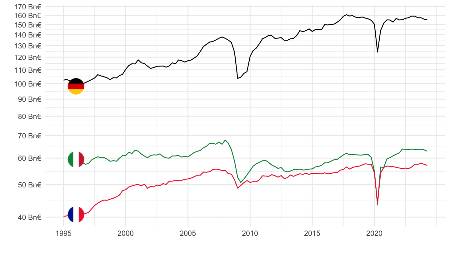
Netherlands, Germany, Spain, France, Italy
Table (% du PIB)
Code
namq_10_a10 %>%
  filter(na_item == "B1G",
         geo %in% c("NL", "DE", "ES", "FR", "IT"),
         unit == "CP_MNAC",
         s_adj == "SCA",
         time == "2021Q3") %>%
  select_if(~ n_distinct(.) > 1) %>%


  select(-geo) %>%
  group_by(Geo) %>%
  mutate(values = round(100* values/ values[nace_r2 == "TOTAL"], 2)) %>%
  mutate(Geo = gsub(" ", "-", str_to_lower(Geo)),
         Geo = paste0('<img src="../../bib/flags/vsmall/', Geo, '.png" alt="Flag">')) %>%
  spread(Geo, values) %>%
  {if (is_html_output()) datatable(., filter = 'top', rownames = F, escape = F) else .}
Table (€)
Code
namq_10_a10 %>%
  filter(na_item == "B1G",
         geo %in% c("NL", "DE", "ES", "FR", "IT"),
         unit == "CP_MNAC",
         s_adj == "SCA",
         time == "2021Q3") %>%
  select_if(~ n_distinct(.) > 1) %>%


  select(-geo) %>%
  mutate(Geo = gsub(" ", "-", str_to_lower(Geo)),
         Geo = paste0('<img src="../../bib/flags/vsmall/', Geo, '.png" alt="Flag">')) %>%
  spread(Geo, values) %>%
  {if (is_html_output()) datatable(., filter = 'top', rownames = F, escape = F) else .}
A - Agriculture, forestry and fishing
Code
namq_10_a10 %>%
  filter(na_item == "B1G",
         nace_r2 %in% c("A", "TOTAL"),
         geo %in% c("NL", "DE", "ES", "FR", "IT"),
         unit == "CP_MNAC",
         s_adj == "SCA") %>%
  quarter_to_date() %>%
  filter(date >= as.Date("1995-01-01")) %>%

  group_by(date) %>%
  mutate(values = values/ values[nace_r2 == "TOTAL"]) %>%
  filter(nace_r2 != "TOTAL") %>%
  mutate(Geo = ifelse(geo == "DE", "Germany", Geo)) %>%
  left_join(colors, by = c("Geo" = "country")) %>%
  mutate(color = ifelse(geo == "NL", color2, color)) %>%
  ggplot(.) + geom_line(aes(x = date, y = values, color = color)) +
  theme_minimal() + xlab("") + ylab("% of GDP") +
  scale_color_identity() + add_flags +
  scale_x_date(breaks = seq(1960, 2100, 2) %>% paste0("-01-01") %>% as.Date,
               labels = date_format("%Y")) +
  scale_y_continuous(breaks = 0.01*seq(-500, 200, 1),
                     labels = percent_format(accuracy = 1))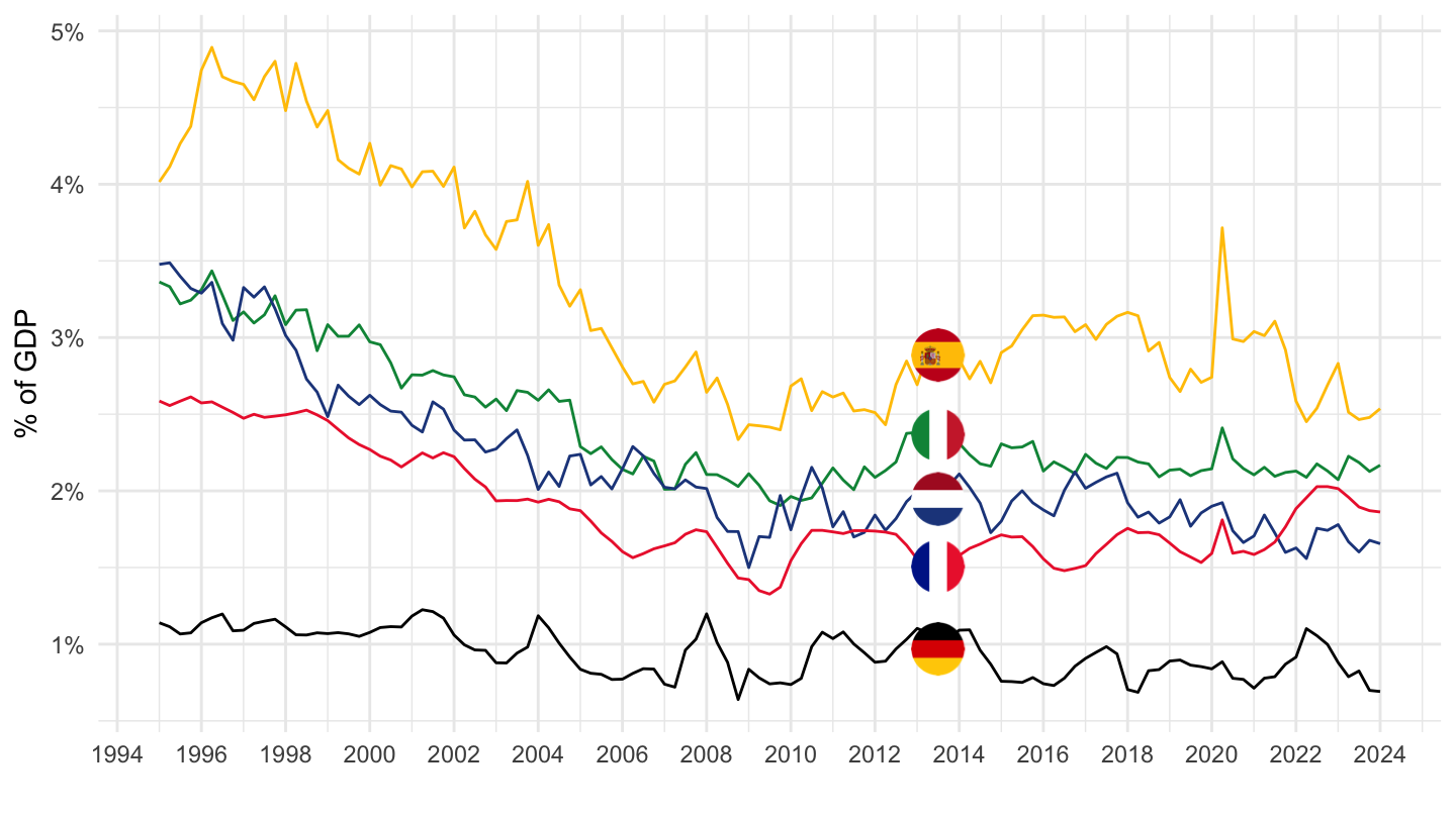
B-E - Industry (except construction)
Code
namq_10_a10 %>%
  filter(na_item == "B1G",
         nace_r2 %in% c("B-E", "TOTAL"),
         geo %in% c("NL", "DE", "ES", "FR", "IT"),
         unit == "CP_MNAC",
         s_adj == "SCA") %>%
  quarter_to_date() %>%
  filter(date >= as.Date("1995-01-01")) %>%

  group_by(date) %>%
  mutate(values = values/ values[nace_r2 == "TOTAL"]) %>%
  filter(nace_r2 != "TOTAL") %>%
  mutate(Geo = ifelse(geo == "DE", "Germany", Geo)) %>%
  left_join(colors, by = c("Geo" = "country")) %>%
  ggplot(.) + geom_line(aes(x = date, y = values, color = color)) +
  theme_minimal() + xlab("") + ylab("% of GDP") +
  scale_color_identity() + add_flags +
  scale_x_date(breaks = seq(1960, 2100, 5) %>% paste0("-01-01") %>% as.Date,
               labels = date_format("%Y")) +
  scale_y_continuous(breaks = 0.01*seq(-500, 200, 1),
                     labels = percent_format(accuracy = 1))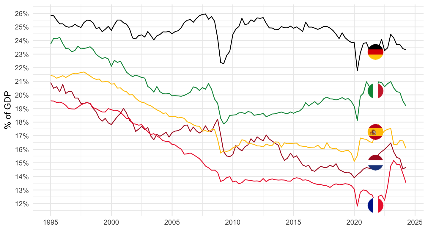
C - Manufacturing Share
Code
namq_10_a10 %>%
  filter(na_item == "B1G",
         nace_r2 %in% c("C", "TOTAL"),
         geo %in% c("NL", "DE", "ES", "FR", "IT"),
         unit == "CP_MNAC",
         s_adj == "SCA") %>%
  quarter_to_date() %>%
  filter(date >= as.Date("1995-01-01")) %>%

  group_by(date) %>%
  mutate(values = values/ values[nace_r2 == "TOTAL"]) %>%
  filter(nace_r2 != "TOTAL") %>%
  mutate(Geo = ifelse(geo == "DE", "Germany", Geo)) %>%
  left_join(colors, by = c("Geo" = "country")) %>%
  ggplot(.) + geom_line(aes(x = date, y = values, color = color)) +
  theme_minimal() + xlab("") + ylab("Industrie Manufacturière (% du PIB)") +
  scale_color_identity() + add_flags +
  scale_x_date(breaks = seq(1960, 2100, 5) %>% paste0("-01-01") %>% as.Date,
               labels = date_format("%Y")) +
  scale_y_continuous(breaks = 0.01*seq(-500, 200, 1),
                     labels = percent_format(accuracy = 1))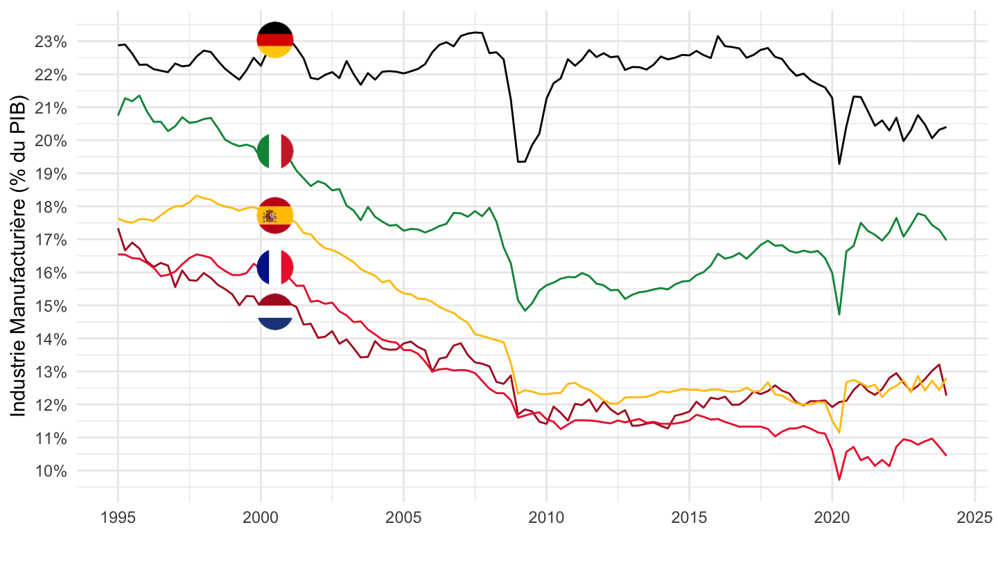
F - Construction
Code
namq_10_a10 %>%
  filter(na_item == "B1G",
         nace_r2 %in% c("F", "TOTAL"),
         geo %in% c("NL", "DE", "ES", "FR", "IT"),
         unit == "CP_MNAC",
         s_adj == "SCA") %>%
  quarter_to_date() %>%
  filter(date >= as.Date("1995-01-01")) %>%

  group_by(date) %>%
  mutate(values = values/ values[nace_r2 == "TOTAL"]) %>%
  filter(nace_r2 != "TOTAL") %>%
  mutate(Geo = ifelse(geo == "DE", "Germany", Geo)) %>%
  left_join(colors, by = c("Geo" = "country")) %>%
  mutate(color = ifelse(geo == "NL", color2, color)) %>%
  ggplot(.) + geom_line(aes(x = date, y = values, color = color)) +
  theme_minimal() + xlab("") + ylab("% of GDP") +
  scale_color_identity() + add_flags +
  scale_x_date(breaks = seq(1960, 2100, 2) %>% paste0("-01-01") %>% as.Date,
               labels = date_format("%Y")) +
  scale_y_continuous(breaks = 0.01*seq(-500, 200, 1),
                     labels = percent_format(accuracy = 1))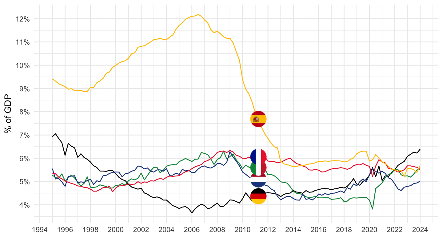
G-I - Wholesale and retail trade, transport, accommodation and food service activities
Code
namq_10_a10 %>%
  filter(na_item == "B1G",
         nace_r2 %in% c("G-I", "TOTAL"),
         geo %in% c("NL", "DE", "ES", "FR", "IT"),
         unit == "CP_MNAC",
         s_adj == "SCA") %>%
  quarter_to_date() %>%
  filter(date >= as.Date("1995-01-01")) %>%

  group_by(date) %>%
  mutate(values = values/ values[nace_r2 == "TOTAL"]) %>%
  filter(nace_r2 != "TOTAL") %>%
  mutate(Geo = ifelse(geo == "DE", "Germany", Geo)) %>%
  left_join(colors, by = c("Geo" = "country")) %>%
  mutate(color = ifelse(geo == "NL", color2, color)) %>%
  ggplot(.) + geom_line(aes(x = date, y = values, color = color)) +
  theme_minimal() + xlab("") + ylab("% of GDP") +
  scale_color_identity() + add_flags +
  scale_x_date(breaks = seq(1960, 2100, 2) %>% paste0("-01-01") %>% as.Date,
               labels = date_format("%Y")) +
  scale_y_continuous(breaks = 0.01*seq(-500, 200, 1),
                     labels = percent_format(accuracy = 1))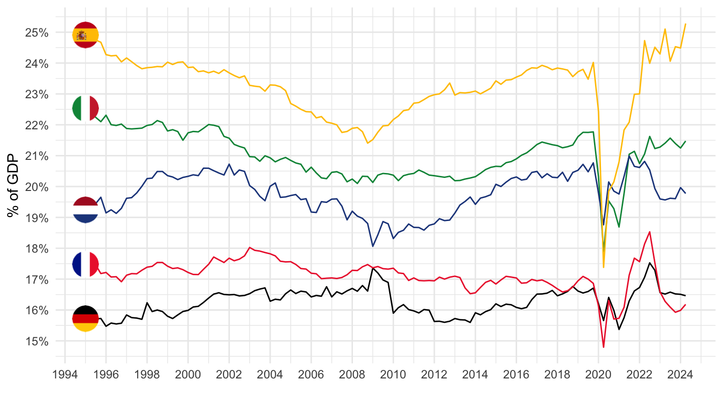
J - Information and communication
Code
namq_10_a10 %>%
  filter(na_item == "B1G",
         nace_r2 %in% c("J", "TOTAL"),
         geo %in% c("NL", "DE", "ES", "FR", "IT"),
         unit == "CP_MNAC",
         s_adj == "SCA") %>%
  quarter_to_date() %>%
  filter(date >= as.Date("1995-01-01")) %>%

  group_by(date) %>%
  mutate(values = values/ values[nace_r2 == "TOTAL"]) %>%
  filter(nace_r2 != "TOTAL") %>%
  mutate(Geo = ifelse(geo == "DE", "Germany", Geo)) %>%
  left_join(colors, by = c("Geo" = "country")) %>%
  mutate(color = ifelse(geo == "NL", color2, color)) %>%
  ggplot(.) + geom_line(aes(x = date, y = values, color = color)) +
  theme_minimal() + xlab("") + ylab("% of GDP") +
  scale_color_identity() + add_flags +
  scale_x_date(breaks = seq(1960, 2100, 2) %>% paste0("-01-01") %>% as.Date,
               labels = date_format("%Y")) +
  scale_y_continuous(breaks = 0.01*seq(-500, 200, .5),
                     labels = percent_format(accuracy = .1))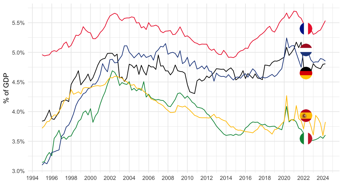
K - Financial and insurance activities
Code
namq_10_a10 %>%
  filter(na_item == "B1G",
         nace_r2 %in% c("K", "TOTAL"),
         geo %in% c("NL", "DE", "ES", "FR", "IT"),
         unit == "CP_MNAC",
         s_adj == "SCA") %>%
  quarter_to_date() %>%
  filter(date >= as.Date("1995-01-01")) %>%

  group_by(date) %>%
  mutate(values = values/ values[nace_r2 == "TOTAL"]) %>%
  filter(nace_r2 != "TOTAL") %>%
  mutate(Geo = ifelse(geo == "DE", "Germany", Geo)) %>%
  left_join(colors, by = c("Geo" = "country")) %>%
  mutate(color = ifelse(geo == "NL", color2, color)) %>%
  ggplot(.) + geom_line(aes(x = date, y = values, color = color)) +
  theme_minimal() + xlab("") + ylab("% of GDP") +
  scale_color_identity() + add_flags +
  scale_x_date(breaks = seq(1960, 2100, 2) %>% paste0("-01-01") %>% as.Date,
               labels = date_format("%Y")) +
  scale_y_continuous(breaks = 0.01*seq(-500, 200, 1),
                     labels = percent_format(accuracy = 1))
L - Real estate activities
Code
namq_10_a10 %>%
  filter(na_item == "B1G",
         nace_r2 %in% c("L", "TOTAL"),
         geo %in% c("NL", "DE", "ES", "FR", "IT"),
         unit == "CP_MNAC",
         s_adj == "SCA") %>%
  quarter_to_date() %>%
  filter(date >= as.Date("1995-01-01")) %>%

  group_by(date) %>%
  mutate(values = values/ values[nace_r2 == "TOTAL"]) %>%
  filter(nace_r2 != "TOTAL") %>%
  mutate(Geo = ifelse(geo == "DE", "Germany", Geo)) %>%
  left_join(colors, by = c("Geo" = "country")) %>%
  mutate(color = ifelse(geo == "NL", color2, color)) %>%
  ggplot(.) + geom_line(aes(x = date, y = values, color = color)) +
  theme_minimal() + xlab("") + ylab("% of GDP") +
  scale_color_identity() + add_flags +
  scale_x_date(breaks = seq(1960, 2100, 2) %>% paste0("-01-01") %>% as.Date,
               labels = date_format("%Y")) +
  scale_y_continuous(breaks = 0.01*seq(-500, 200, 1),
                     labels = percent_format(accuracy = 1))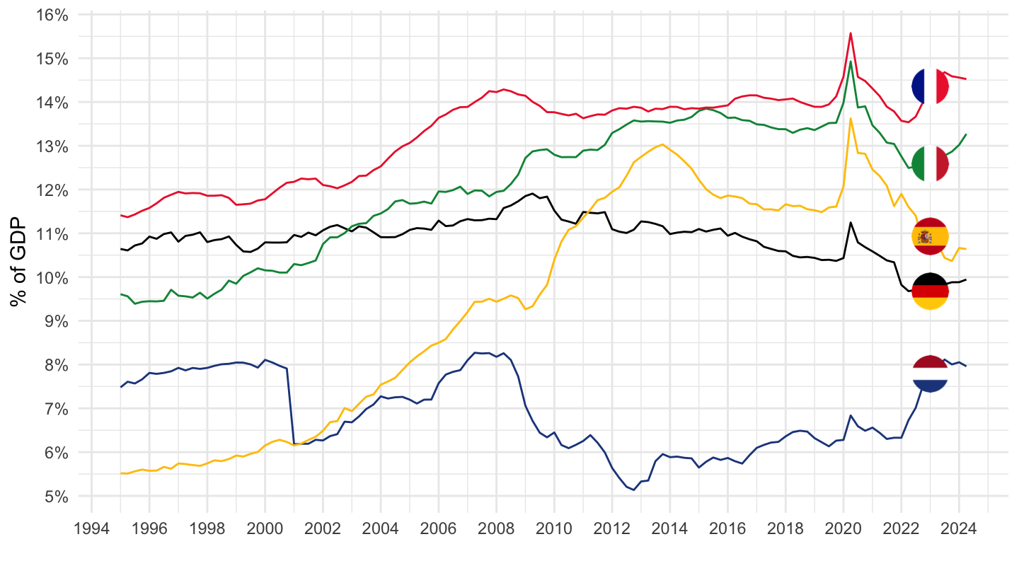
M_N - Professional, scientific and technical activities; administrative and support service activities
Code
namq_10_a10 %>%
  filter(na_item == "B1G",
         nace_r2 %in% c("M_N", "TOTAL"),
         geo %in% c("NL", "DE", "ES", "FR", "IT"),
         unit == "CP_MNAC",
         s_adj == "SCA") %>%
  quarter_to_date() %>%
  filter(date >= as.Date("1995-01-01")) %>%

  group_by(date) %>%
  mutate(values = values/ values[nace_r2 == "TOTAL"]) %>%
  filter(nace_r2 != "TOTAL") %>%
  mutate(Geo = ifelse(geo == "DE", "Germany", Geo)) %>%
  left_join(colors, by = c("Geo" = "country")) %>%
  mutate(color = ifelse(geo == "NL", color2, color)) %>%
  ggplot(.) + geom_line(aes(x = date, y = values, color = color)) +
  theme_minimal() + xlab("") + ylab("% of GDP") +
  scale_color_identity() + add_flags +
  scale_x_date(breaks = seq(1960, 2100, 2) %>% paste0("-01-01") %>% as.Date,
               labels = date_format("%Y")) +
  scale_y_continuous(breaks = 0.01*seq(-500, 200, 1),
                     labels = percent_format(accuracy = 1))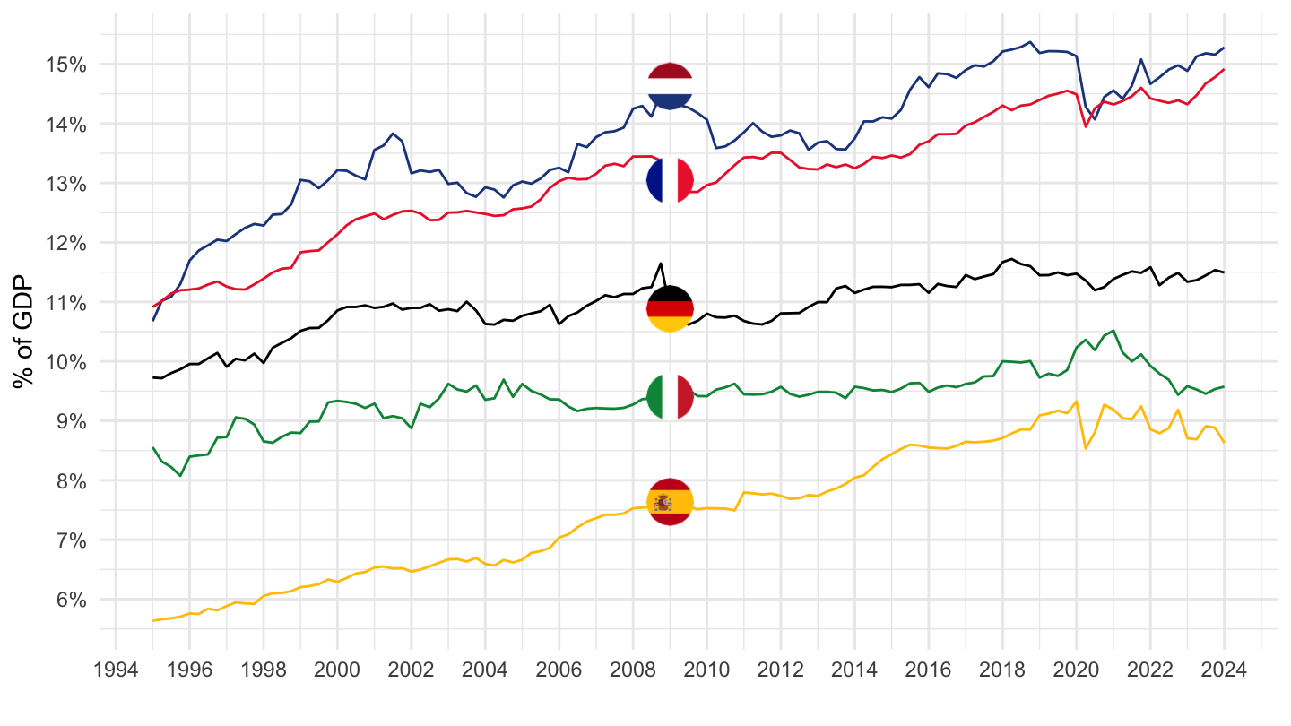
O-Q - Public administration, defence, education, human health and social work activities
Code
namq_10_a10 %>%
  filter(na_item == "B1G",
         nace_r2 %in% c("O-Q", "TOTAL"),
         geo %in% c("NL", "DE", "ES", "FR", "IT"),
         unit == "CP_MNAC",
         s_adj == "SCA") %>%
  quarter_to_date() %>%
  filter(date >= as.Date("1995-01-01")) %>%

  group_by(date) %>%
  mutate(values = values/ values[nace_r2 == "TOTAL"]) %>%
  filter(nace_r2 != "TOTAL") %>%
  mutate(Geo = ifelse(geo == "DE", "Germany", Geo)) %>%
  left_join(colors, by = c("Geo" = "country")) %>%
  mutate(color = ifelse(geo == "NL", color2, color)) %>%
  ggplot(.) + geom_line(aes(x = date, y = values, color = color)) +
  theme_minimal() + xlab("") + ylab("% of GDP") +
  scale_color_identity() + add_flags +
  scale_x_date(breaks = seq(1960, 2100, 2) %>% paste0("-01-01") %>% as.Date,
               labels = date_format("%Y")) +
  scale_y_continuous(breaks = 0.01*seq(-500, 200, 1),
                     labels = percent_format(accuracy = 1))
R-U - Arts, entertainment and recreation; other service activities; activities of household and extra-territorial organizations and bodies
Code
namq_10_a10 %>%
  filter(na_item == "B1G",
         nace_r2 %in% c("R-U", "TOTAL"),
         geo %in% c("NL", "DE", "ES", "FR", "IT"),
         unit == "CP_MNAC",
         s_adj == "SCA") %>%
  quarter_to_date() %>%
  filter(date >= as.Date("1995-01-01")) %>%

  group_by(date) %>%
  mutate(values = values/ values[nace_r2 == "TOTAL"]) %>%
  filter(nace_r2 != "TOTAL") %>%
  mutate(Geo = ifelse(geo == "DE", "Germany", Geo)) %>%
  left_join(colors, by = c("Geo" = "country")) %>%
  mutate(color = ifelse(geo == "NL", color2, color)) %>%
  ggplot(.) + geom_line(aes(x = date, y = values, color = color)) +
  theme_minimal() + xlab("") + ylab("% of GDP") +
  scale_color_identity() + add_flags +
  scale_x_date(breaks = seq(1960, 2100, 2) %>% paste0("-01-01") %>% as.Date,
               labels = date_format("%Y")) +
  scale_y_continuous(breaks = 0.01*seq(-500, 200, 1),
                     labels = percent_format(accuracy = 1))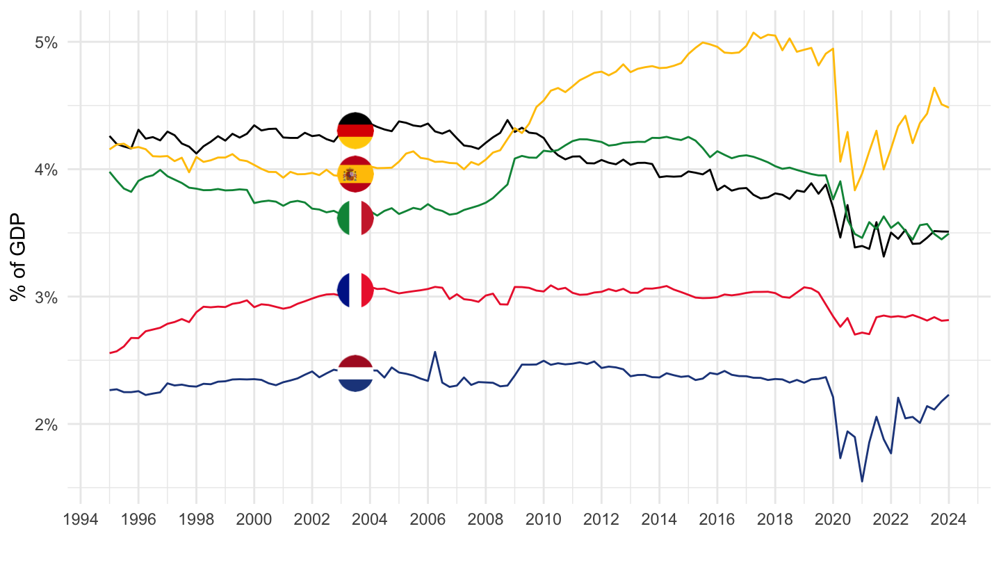
Industry and Manufacturing Share
France, Germany, Italy, Spain, Netherlands, Euro area
1995-
Code
load_data("eurostat/nace_r2_fr.RData")
namq_10_a10 %>%
  filter(na_item == "B1G",
         nace_r2 %in% c("C", "TOTAL", "B-E"),
         geo %in% c("FR", "DE", "IT", "ES", "EA"),
         unit == "CP_MNAC",
         s_adj == "SCA") %>%
  quarter_to_date() %>%


  group_by(date) %>%
  mutate(values = values/ values[nace_r2 == "TOTAL"]) %>%
  filter(nace_r2 != "TOTAL",
         date >= as.Date("1995-01-01")) %>%
  mutate(Geo = ifelse(geo == "DE", "Germany", Geo)) %>%
  mutate(Geo = ifelse(geo == "EA", "Europe", Geo)) %>%
  left_join(colors, by = c("Geo" = "country")) %>%
  ggplot(.) + geom_line(aes(x = date, y = values, color = color, linetype = Nace_r2)) +
  scale_color_identity() +
  scale_linetype_manual(values = c("dashed","solid")) +
  theme_minimal() +
  scale_x_date(breaks = seq(1920, 2100, 2) %>% paste0("-01-01") %>% as.Date,
               labels = date_format("%Y")) +
  theme(legend.position = c(0.2, 0.1),
        legend.title = element_blank()) +
  add_flags +
  scale_y_continuous(breaks = 0.01*seq(-60, 60, 1),
                     labels = scales::percent_format(accuracy = 1)) +
  ylab("VA Manufacturière, Industrielle (% du PIB)") + xlab("")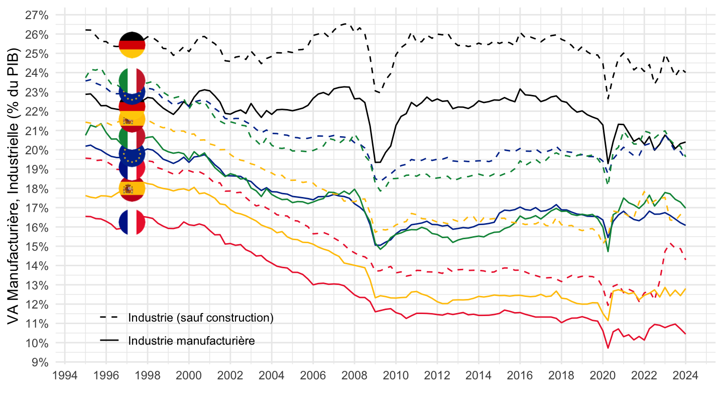
Manufacturing Share (% of GDP)
Table: All Countries
Code
namq_10_a10 %>%
  filter(na_item == "B1G",
         nace_r2 %in% c("C", "TOTAL"),
         time %in% c("2019Q4", "2014Q4", "2009Q4", "2004Q4", "1999Q4", "1994Q4"),
         unit == "CP_MNAC",
         s_adj == "SCA") %>%

  group_by(time, geo) %>%
  mutate(values = round(100*values/ values[nace_r2 == "TOTAL"], 1) %>% paste0("%")) %>%
  filter(nace_r2 != "TOTAL") %>%
  select(geo, Geo, time, values) %>%
  spread(time, values) %>%
  mutate(Geo = ifelse(geo == "DE", "Germany", Geo)) %>%
  mutate(Flag = gsub(" ", "-", str_to_lower(Geo)),
         Flag = paste0('<img src="../../bib/flags/vsmall/', Flag, '.png" alt="Flag">')) %>%
  select(Flag, everything()) %>%
  {if (is_html_output()) datatable(., filter = 'top', rownames = F, escape = F) else .}
France, Germany, Italy
All
Code
namq_10_a10 %>%
  filter(na_item == "B1G",
         nace_r2 %in% c("C", "TOTAL"),
         geo %in% c("FR", "DE", "IT"),
         unit == "CP_MNAC",
         s_adj == "SCA") %>%
  quarter_to_date() %>%

  group_by(date) %>%
  mutate(values = values/ values[nace_r2 == "TOTAL"]) %>%
  filter(nace_r2 != "TOTAL") %>%
  mutate(Geo = ifelse(geo == "DE", "Germany", Geo)) %>%
  left_join(colors, by = c("Geo" = "country")) %>%
  ggplot(.) + geom_line(aes(x = date, y = values, color = color)) +
  theme_minimal() + xlab("") + ylab("% of GDP") +
  scale_color_identity() + add_flags +
  scale_x_date(breaks = seq(1960, 2100, 5) %>% paste0("-01-01") %>% as.Date,
               labels = date_format("%Y")) +
  scale_y_continuous(breaks = 0.01*seq(-500, 200, 1),
                     labels = percent_format(accuracy = 1))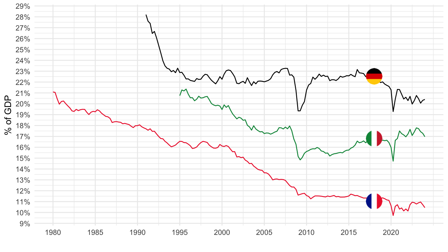
1995-
Code
namq_10_a10 %>%
  filter(na_item == "B1G",
         nace_r2 %in% c("C", "B-E", "TOTAL"),
         geo %in% c("FR", "DE", "IT"),
         unit == "CP_MNAC",
         s_adj == "SCA") %>%
  quarter_to_date() %>%

  group_by(date) %>%
  mutate(values = values / values[nace_r2 == "TOTAL"]) %>%
  filter(nace_r2 != "TOTAL",
         date >= as.Date("1995-01-01")) %>%
  mutate(Geo = ifelse(geo == "DE", "Germany", Geo)) %>%
  left_join(colors, by = c("Geo" = "country")) %>%
  ggplot(.) + geom_line(aes(x = date, y = values, color = color, linetype = nace_r2)) +
  theme_minimal() + xlab("") + ylab("% of GDP") +
  scale_color_identity() + add_flags +
  scale_x_date(breaks = seq(1960, 2100, 5) %>% paste0("-01-01") %>% as.Date,
               labels = date_format("%Y")) +
  scale_y_continuous(breaks = 0.01*seq(-500, 200, 1),
                     labels = percent_format(accuracy = 1))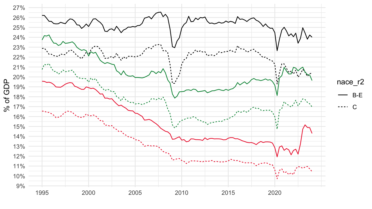
Poland, Spain, Austria
Code
namq_10_a10 %>%
  filter(na_item == "B1G",
         nace_r2 %in% c("C", "TOTAL"),
         geo %in% c("PL", "ES", "AT"),
         unit == "CP_MNAC",
         s_adj == "SCA") %>%
  quarter_to_date() %>%

  group_by(date) %>%
  mutate(values = values/ values[nace_r2 == "TOTAL"]) %>%
  filter(nace_r2 != "TOTAL") %>%
  left_join(colors, by = c("Geo" = "country")) %>%
  ggplot(.) + geom_line(aes(x = date, y = values, color = color)) +
  theme_minimal() + xlab("") + ylab("% of GDP") +
  scale_color_identity() + add_flags +
  scale_x_date(breaks = seq(1960, 2100, 5) %>% paste0("-01-01") %>% as.Date,
               labels = date_format("%Y")) +
  scale_y_continuous(breaks = 0.01*seq(-500, 200, 1),
                     labels = percent_format(accuracy = 1))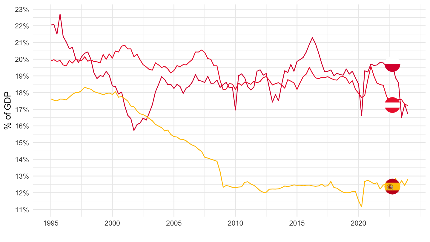
Greece, Spain, Austria
Code
namq_10_a10 %>%
  filter(na_item == "B1G",
         nace_r2 %in% c("C", "TOTAL"),
         geo %in% c("EL", "RS", "RO"),
         unit == "CP_MNAC",
         s_adj == "SCA") %>%
  quarter_to_date() %>%

  group_by(date) %>%
  mutate(values = values/ values[nace_r2 == "TOTAL"]) %>%
  filter(nace_r2 != "TOTAL") %>%
  left_join(colors, by = c("Geo" = "country")) %>%
  ggplot(.) + geom_line(aes(x = date, y = values, color = color)) +
  theme_minimal() + xlab("") + ylab("% of GDP") +
  scale_color_identity() + add_flags +
  scale_x_date(breaks = seq(1960, 2100, 5) %>% paste0("-01-01") %>% as.Date,
               labels = date_format("%Y")) +
  scale_y_continuous(breaks = 0.01*seq(-500, 200, 1),
                     labels = percent_format(accuracy = 1))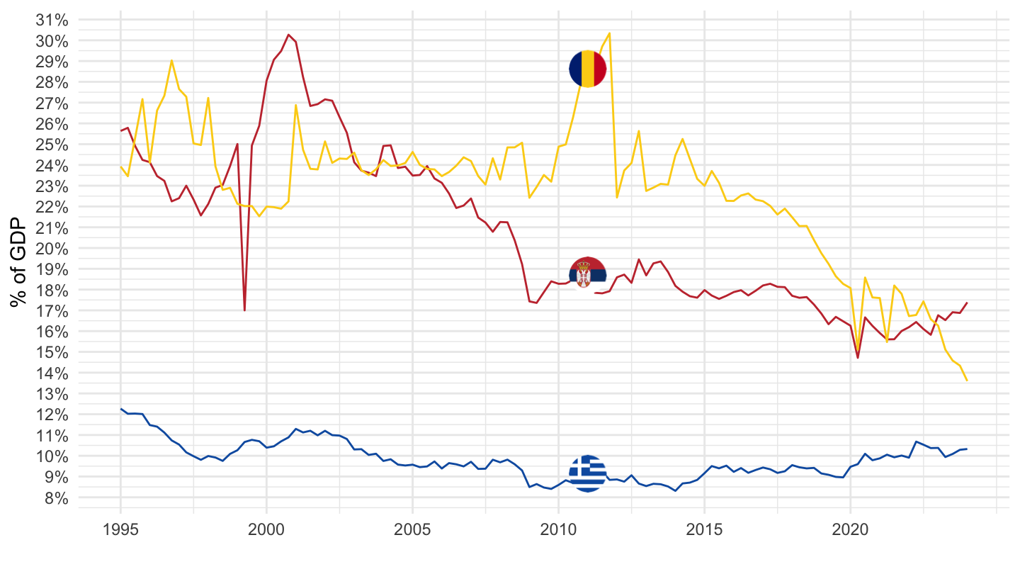
Italy, Germany, Spain, France, Netherlands
1990-
Code
namq_10_a10 %>%
  filter(na_item == "B1G",
         nace_r2 %in% c("C", "TOTAL"),
         geo %in% c("NL", "DE", "ES", "FR", "IT"),
         unit == "CP_MNAC",
         s_adj == "SCA") %>%
  quarter_to_date() %>%
  filter(date >= as.Date("1990-01-01")) %>%

  group_by(date) %>%
  mutate(values = values/ values[nace_r2 == "TOTAL"]) %>%
  filter(nace_r2 != "TOTAL") %>%
  mutate(Geo = ifelse(geo == "DE", "Germany", Geo)) %>%
  left_join(colors, by = c("Geo" = "country")) %>%
  mutate(color = ifelse(geo == "NL", color2, color)) %>%
  ggplot(.) + geom_line(aes(x = date, y = values, color = color)) +
  theme_minimal() + xlab("") + ylab("% du PIB") +
  scale_color_identity() + add_flags +
  scale_x_date(breaks = seq(1960, 2100, 5) %>% paste0("-01-01") %>% as.Date,
               labels = date_format("%Y")) +
  scale_y_continuous(breaks = 0.01*seq(0, 30, 1),
                     labels = percent_format(accuracy = 1))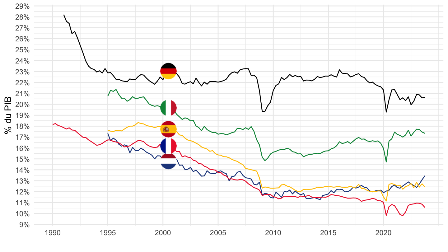
1995-
Code
namq_10_a10 %>%
  filter(na_item == "B1G",
         nace_r2 %in% c("C", "TOTAL"),
         geo %in% c("NL", "DE", "ES", "FR", "IT"),
         unit == "CP_MNAC",
         s_adj == "SCA") %>%
  quarter_to_date() %>%
  filter(date >= as.Date("1995-01-01")) %>%

  group_by(date) %>%
  mutate(values = values/ values[nace_r2 == "TOTAL"]) %>%
  filter(nace_r2 != "TOTAL") %>%
  mutate(Geo = ifelse(geo == "DE", "Germany", Geo)) %>%
  left_join(colors, by = c("Geo" = "country")) %>%
  mutate(color = ifelse(geo == "NL", color2, color)) %>%
  ggplot(.) + geom_line(aes(x = date, y = values, color = color)) +
  theme_minimal() + xlab("") + ylab("% of GDP") +
  scale_color_identity() + add_flags +
  scale_x_date(breaks = seq(1960, 2100, 2) %>% paste0("-01-01") %>% as.Date,
               labels = date_format("%Y")) +
  scale_y_continuous(breaks = 0.01*seq(-500, 200, 1),
                     labels = percent_format(accuracy = 1))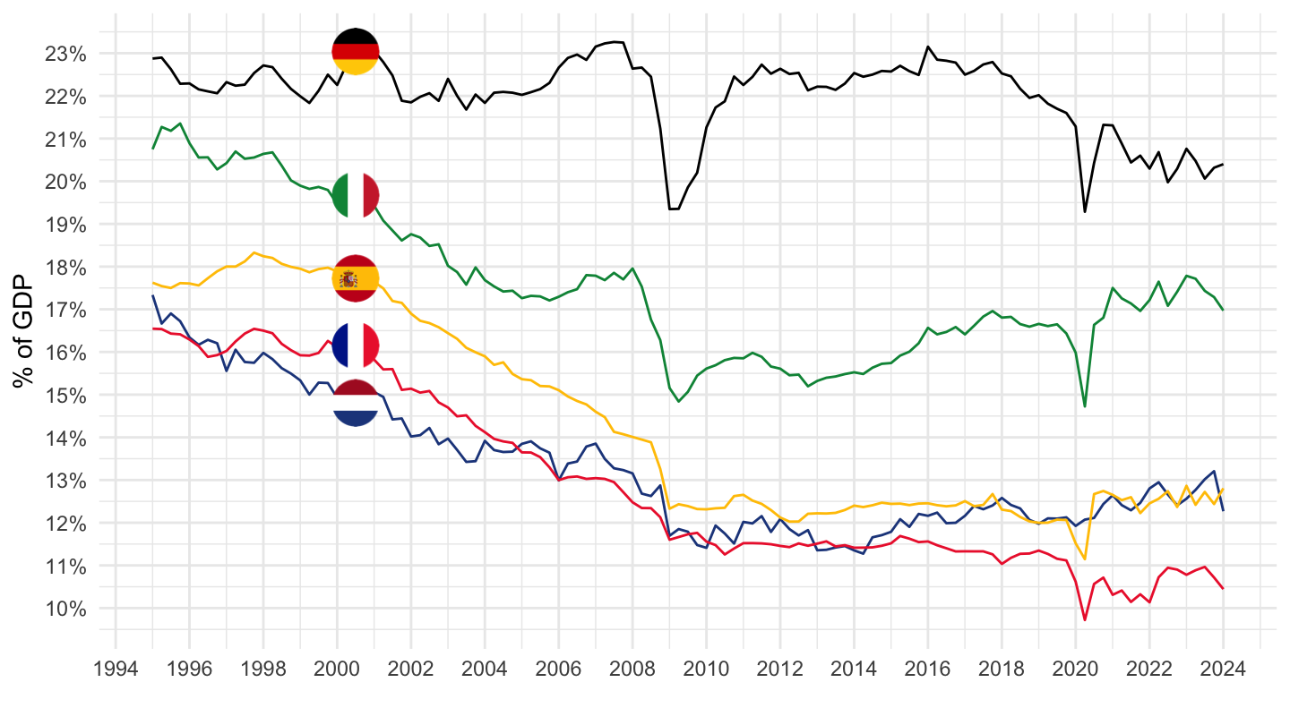
Denmark, Sweden, Switzerland
Code
namq_10_a10 %>%
  filter(na_item == "B1G",
         nace_r2 %in% c("C", "TOTAL"),
         geo %in% c("DK", "SE", "CH"),
         unit == "CP_MNAC",
         s_adj == "SCA") %>%
  quarter_to_date() %>%
  filter(date >= as.Date("1990-01-01")) %>%

  group_by(date) %>%
  mutate(values = values/ values[nace_r2 == "TOTAL"]) %>%
  filter(nace_r2 != "TOTAL") %>%
  mutate(Geo = ifelse(geo == "DE", "Allemagne", Geo)) %>%
  left_join(colors, by = c("Geo" = "country")) %>%
  ggplot(.) + geom_line(aes(x = date, y = values, color = color)) +
  theme_minimal() + xlab("") + ylab("% of GDP") +
  scale_color_identity() + add_flags +
  scale_x_date(breaks = seq(1960, 2100, 5) %>% paste0("-01-01") %>% as.Date,
               labels = date_format("%Y")) +
  scale_y_continuous(breaks = 0.01*seq(-500, 200, 1),
                     labels = percent_format(accuracy = 1))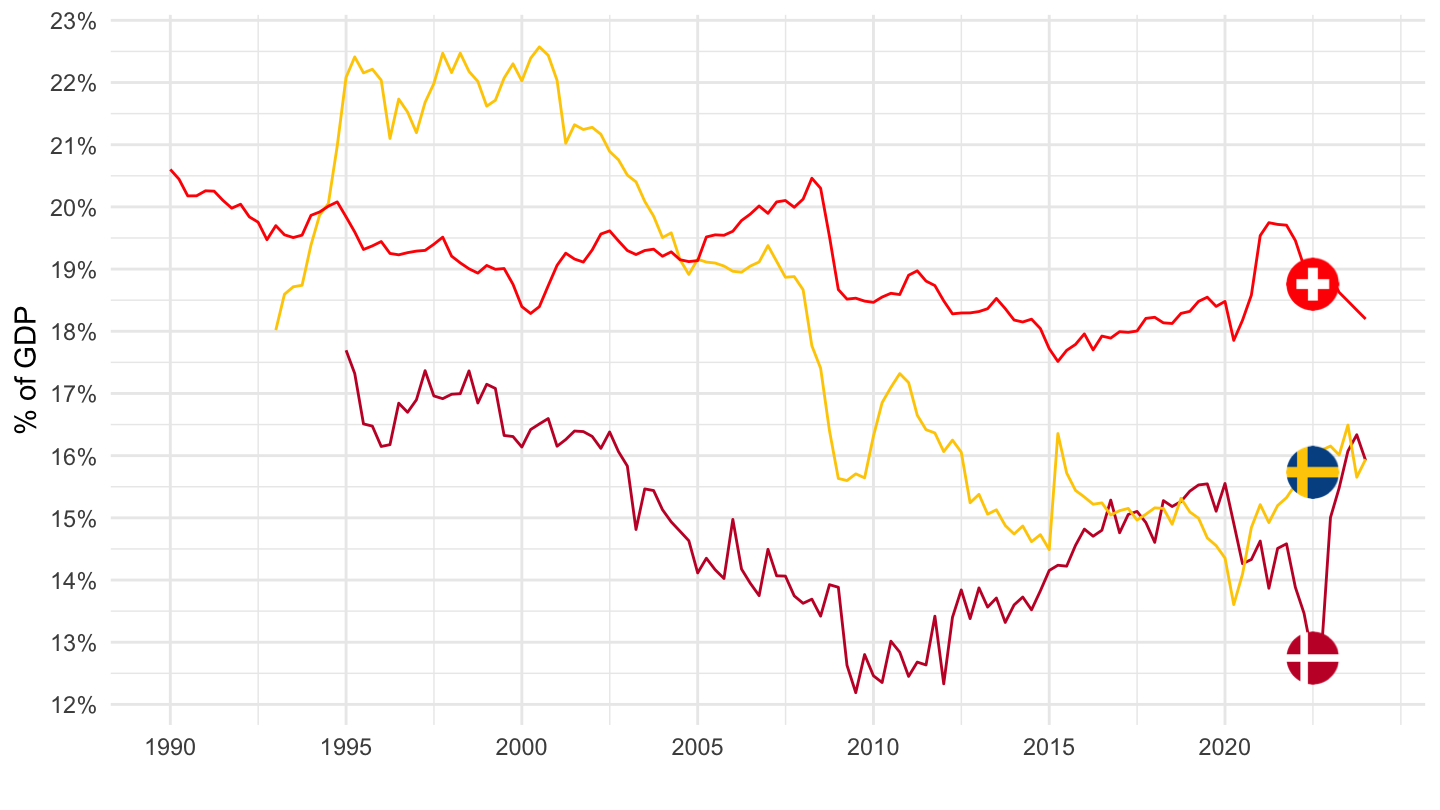
Euro Area, Europe
Code
load_data("eurostat/geo.RData")
namq_10_a10 %>%
  filter(na_item == "B1G",
         nace_r2 %in% c("C", "TOTAL"),
         geo %in% c("EA19", "EU15", "EU28", "EU27_2020", "EA", "EA12"),
         unit == "CP_MNAC",
         s_adj == "SCA") %>%
  quarter_to_date() %>%

  group_by(date) %>%
  mutate(values = values/ values[nace_r2 == "TOTAL"]) %>%
  filter(nace_r2 != "TOTAL") %>%
  left_join(colors, by = c("Geo" = "country")) %>%
  ggplot(.) + geom_line(aes(x = date, y = values, color = color)) +
  theme_minimal() + xlab("") + ylab("% of GDP") +
  scale_color_identity() + add_flags +
  scale_x_date(breaks = seq(1960, 2100, 5) %>% paste0("-01-01") %>% as.Date,
               labels = date_format("%Y")) +
  scale_y_continuous(breaks = 0.01*seq(-500, 200, 1),
                     labels = percent_format(accuracy = 1),
                     limits = c(0.14, 0.21)) +
  theme(legend.position = c(0.6, 0.75),
        legend.title = element_blank())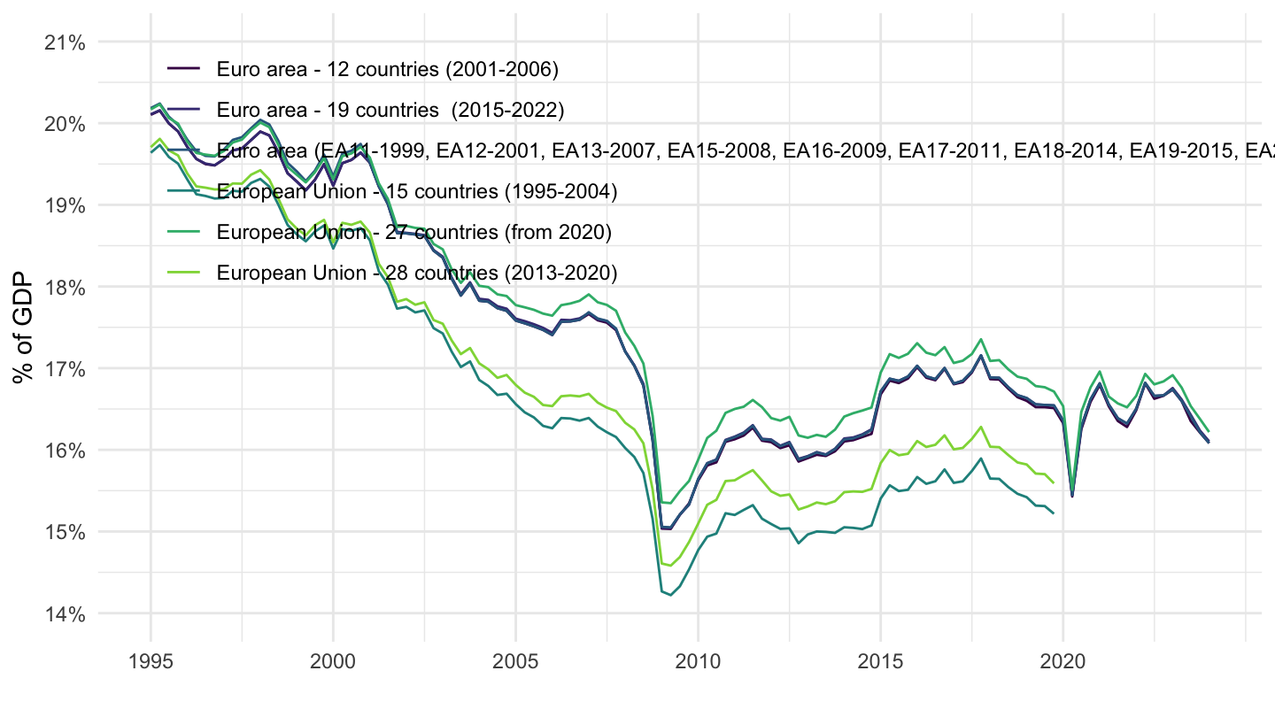
Industry and Manufacturing Share
France, Germany, Italy
1995- (Flags)
Code
namq_10_a10 %>%
  filter(na_item == "B1G",
         nace_r2 %in% c("C", "B-E", "TOTAL"),
         geo %in% c("FR", "DE", "IT"),
         unit == "CP_MNAC",
         s_adj == "SCA") %>%
  quarter_to_date() %>%

  group_by(date) %>%
  mutate(values = values/ values[nace_r2 == "TOTAL"]) %>%
  filter(nace_r2 != "TOTAL",
         date >= as.Date("1995-01-01")) %>%
  mutate(Geo = ifelse(geo == "DE", "Germany", Geo)) %>%
  left_join(colors, by = c("Geo" = "country")) %>%
  ggplot(.) + geom_line(aes(x = date, y = values, color = color, linetype = nace_r2)) +
  scale_color_identity() +
  scale_linetype_manual(values = c("solid", "dashed")) +
  theme_minimal() +
  scale_x_date(breaks = seq(1920, 2100, 2) %>% paste0("-01-01") %>% as.Date,
               labels = date_format("%Y")) +
  theme(legend.position = "none") +
  add_flags +
  scale_y_continuous(breaks = 0.01*seq(-60, 60, 2),
                     labels = scales::percent_format(accuracy = 1)) +
  ylab("VA Manufacturière, Industrielle (% du PIB)") + xlab("")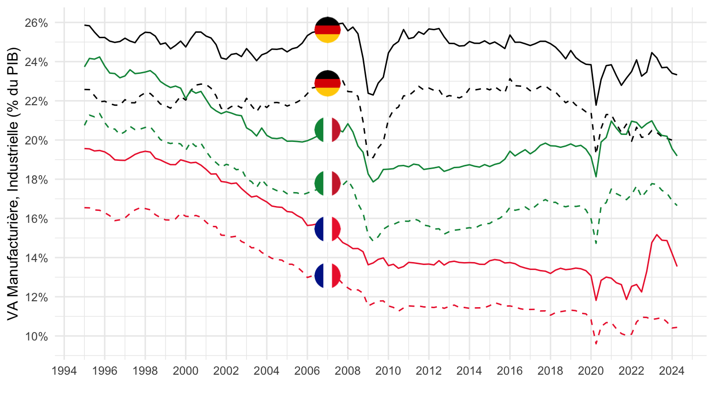
% of GDP
France
Code
namq_10_a10 %>%
  filter(na_item == "B1G",
         nace_r2 %in% c("C", "TOTAL", "L", "F"),
         geo %in% c("FR"),
         unit == "CP_MNAC",
         s_adj == "SCA") %>%
  quarter_to_date() %>%

  select(nace_r2, Nace_r2, date, values) %>%
  group_by(date) %>%
  mutate(values = values/ values[nace_r2 == "TOTAL"]) %>%
  filter(nace_r2 != "TOTAL")  %>%
  ggplot(.) + geom_line(aes(x = date, y = values, color = Nace_r2)) +
  theme_minimal() + xlab("") + ylab("% of GDP") +
  scale_color_manual(values = viridis(4)[1:3]) +
  scale_x_date(breaks = seq(1960, 2100, 5) %>% paste0("-01-01") %>% as.Date,
               labels = date_format("%Y")) +
  scale_y_continuous(breaks = 0.01*seq(-500, 200, 1),
                     labels = percent_format(accuracy = 1)) +
  theme(legend.position = c(0.75, 0.85),
        legend.title = element_blank())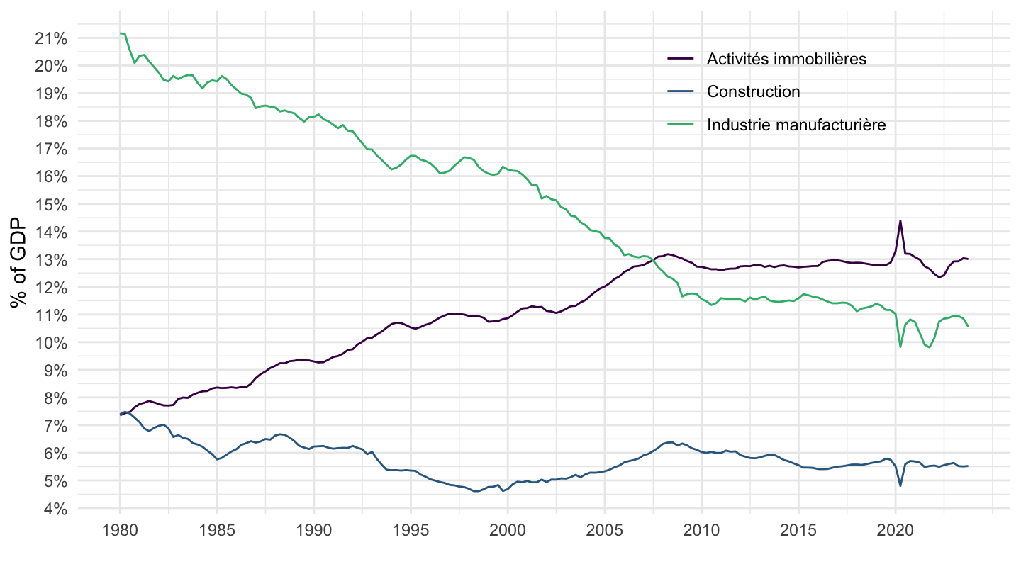
France (1995-)
Code
namq_10_a10 %>%
  filter(na_item == "B1G",
         nace_r2 %in% c("C", "TOTAL", "L", "Q", "F"),
         geo %in% c("FR"),
         unit == "CP_MNAC",
         s_adj == "SCA") %>%
  quarter_to_date() %>%
  filter(date >= as.Date("1995-01-01")) %>%

  select(nace_r2, Nace_r2, date, values) %>%
  group_by(date) %>%
  mutate(values = values/ values[nace_r2 == "TOTAL"]) %>%
  filter(nace_r2 != "TOTAL")  %>%
  ggplot(.) + geom_line(aes(x = date, y = values, color = Nace_r2)) +
  theme_minimal() + xlab("") + ylab("% of GDP") +
  scale_color_manual(values = viridis(4)[1:3]) +
  scale_x_date(breaks = seq(1960, 2100, 5) %>% paste0("-01-01") %>% as.Date,
               labels = date_format("%Y")) +
  scale_y_continuous(breaks = 0.01*seq(0, 30, 2),
                     labels = percent_format(accuracy = 1),
                     limits = c(0, 0.3)) +
  theme(legend.position = c(0.75, 0.85),
        legend.title = element_blank())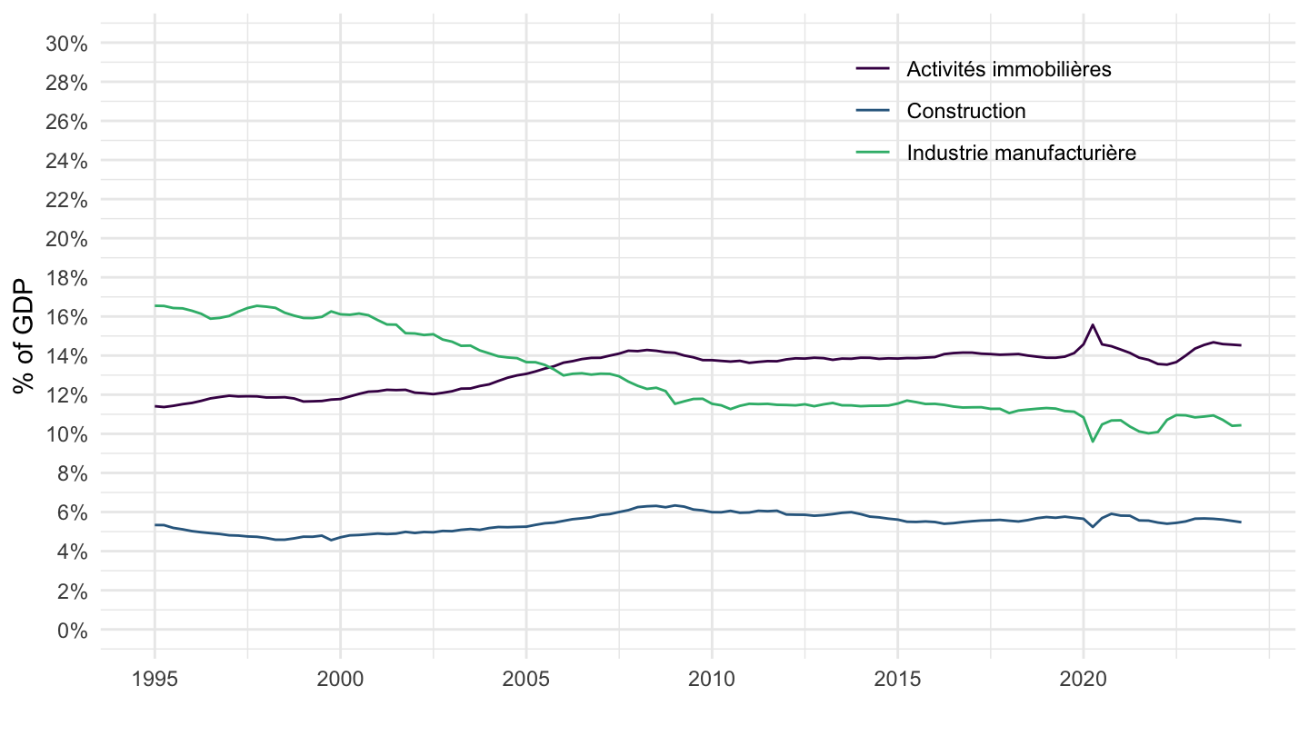
Germany
Code
namq_10_a10 %>%
  filter(na_item == "B1G",
         nace_r2 %in% c("C", "TOTAL", "L", "Q", "F"),
         geo %in% c("DE"),
         unit == "CP_MNAC",
         s_adj == "SCA") %>%
  quarter_to_date() %>%

  select(nace_r2, Nace_r2, date, values) %>%
  group_by(date) %>%
  mutate(values = values/ values[nace_r2 == "TOTAL"]) %>%
  filter(nace_r2 != "TOTAL")  %>%
  ggplot(.) + geom_line(aes(x = date, y = values, color = Nace_r2)) +
  theme_minimal() + xlab("") + ylab("% of GDP") +
  scale_color_manual(values = viridis(4)[1:3]) +
  scale_x_date(breaks = seq(1960, 2100, 5) %>% paste0("-01-01") %>% as.Date,
               labels = date_format("%Y")) +
  scale_y_continuous(breaks = 0.01*seq(0, 30, 2),
                     labels = percent_format(accuracy = 1),
                     limits = c(0, 0.3)) +
  theme(legend.position = c(0.75, 0.85),
        legend.title = element_blank())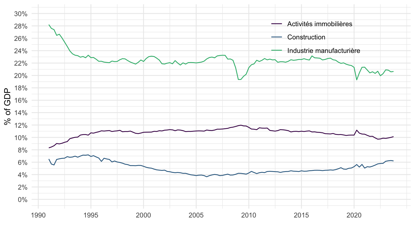
Italy
Code
namq_10_a10 %>%
  filter(na_item == "B1G",
         nace_r2 %in% c("C", "TOTAL", "L", "Q", "F"),
         geo %in% c("IT"),
         unit == "CP_MNAC",
         s_adj == "SCA") %>%
  quarter_to_date() %>%

  select(nace_r2, Nace_r2, date, values) %>%
  group_by(date) %>%
  mutate(values = values/ values[nace_r2 == "TOTAL"]) %>%
  filter(nace_r2 != "TOTAL")  %>%
  ggplot(.) + geom_line(aes(x = date, y = values, color = Nace_r2)) +
  theme_minimal() + xlab("") + ylab("% of GDP") +
  scale_color_manual(values = viridis(4)[1:3]) +
  scale_x_date(breaks = seq(1960, 2100, 5) %>% paste0("-01-01") %>% as.Date,
               labels = date_format("%Y")) +
  scale_y_continuous(breaks = 0.01*seq(-500, 200, 1),
                     labels = percent_format(accuracy = 1)) +
  theme(legend.position = c(0.75, 0.85),
        legend.title = element_blank())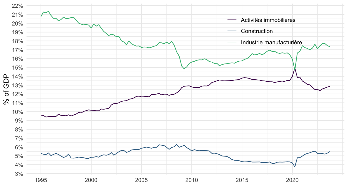
Spain
Code
namq_10_a10 %>%
  filter(na_item == "B1G",
         nace_r2 %in% c("C", "TOTAL", "L", "Q", "F"),
         geo %in% c("ES"),
         unit == "CP_MNAC",
         s_adj == "SCA") %>%
  quarter_to_date() %>%

  select(nace_r2, Nace_r2, date, values) %>%
  group_by(date) %>%
  mutate(values = values/ values[nace_r2 == "TOTAL"]) %>%
  filter(nace_r2 != "TOTAL")  %>%
  ggplot(.) + geom_line(aes(x = date, y = values, color = Nace_r2)) +
  theme_minimal() + xlab("") + ylab("% of GDP") +
  scale_color_manual(values = viridis(4)[1:3]) +
  scale_x_date(breaks = seq(1960, 2100, 5) %>% paste0("-01-01") %>% as.Date,
               labels = date_format("%Y")) +
  scale_y_continuous(breaks = 0.01*seq(-500, 200, 1),
                     labels = percent_format(accuracy = 1)) +
  theme(legend.position = c(0.75, 0.85),
        legend.title = element_blank())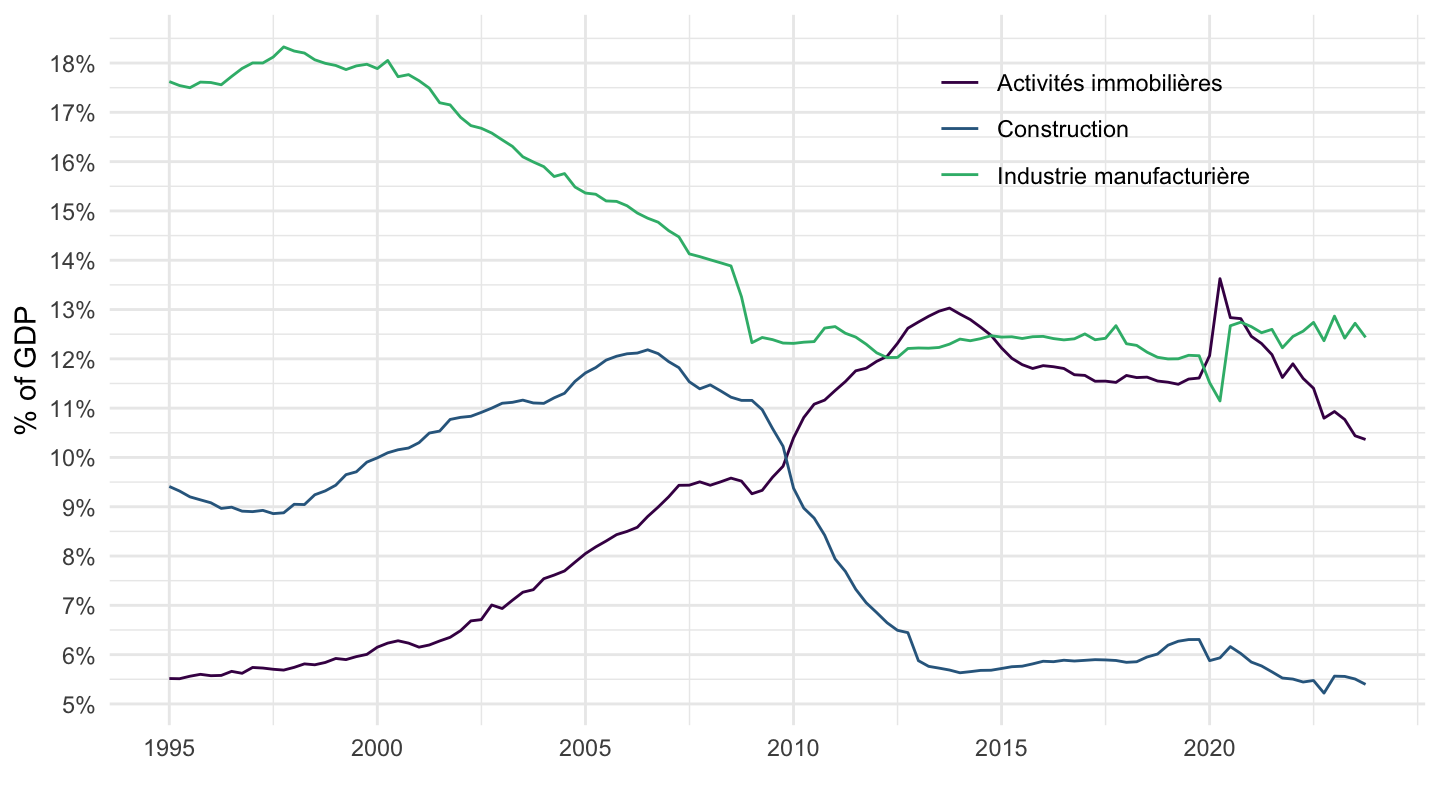
Greece
Code
namq_10_a10 %>%
  filter(na_item == "B1G",
         nace_r2 %in% c("C", "TOTAL", "L", "Q", "F"),
         geo %in% c("EL"),
         unit == "CP_MNAC",
         s_adj == "SCA") %>%
  quarter_to_date() %>%

  select(nace_r2, Nace_r2, date, values) %>%
  group_by(date) %>%
  mutate(values = values/ values[nace_r2 == "TOTAL"]) %>%
  filter(nace_r2 != "TOTAL")  %>%
  ggplot(.) + geom_line(aes(x = date, y = values, color = Nace_r2)) +
  theme_minimal() + xlab("") + ylab("% of GDP") +
  scale_color_manual(values = viridis(4)[1:3]) +
  scale_x_date(breaks = seq(1960, 2100, 5) %>% paste0("-01-01") %>% as.Date,
               labels = date_format("%Y")) +
  scale_y_continuous(breaks = 0.01*seq(-500, 200, 1),
                     labels = percent_format(accuracy = 1)) +
  theme(legend.position = c(0.25, 0.85),
        legend.title = element_blank())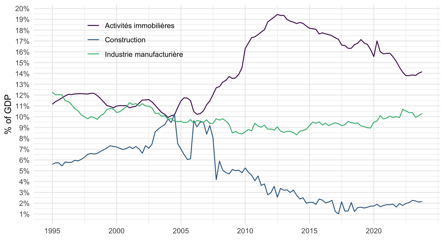
Netherlands
Code
namq_10_a10 %>%
  filter(na_item == "B1G",
         nace_r2 %in% c("C", "TOTAL", "L", "Q", "F"),
         geo %in% c("NL"),
         unit == "CP_MNAC",
         s_adj == "SCA") %>%
  quarter_to_date() %>%

  select(nace_r2, Nace_r2, date, values) %>%
  group_by(date) %>%
  mutate(values = values/ values[nace_r2 == "TOTAL"]) %>%
  filter(nace_r2 != "TOTAL")  %>%
  ggplot(.) + geom_line(aes(x = date, y = values, color = Nace_r2)) +
  theme_minimal() + xlab("") + ylab("% of GDP") +
  scale_color_manual(values = viridis(4)[1:3]) +
  scale_x_date(breaks = seq(1960, 2100, 5) %>% paste0("-01-01") %>% as.Date,
               labels = date_format("%Y")) +
  scale_y_continuous(breaks = 0.01*seq(-500, 200, 1),
                     labels = percent_format(accuracy = 1)) +
  theme(legend.position = c(0.75, 0.85),
        legend.title = element_blank())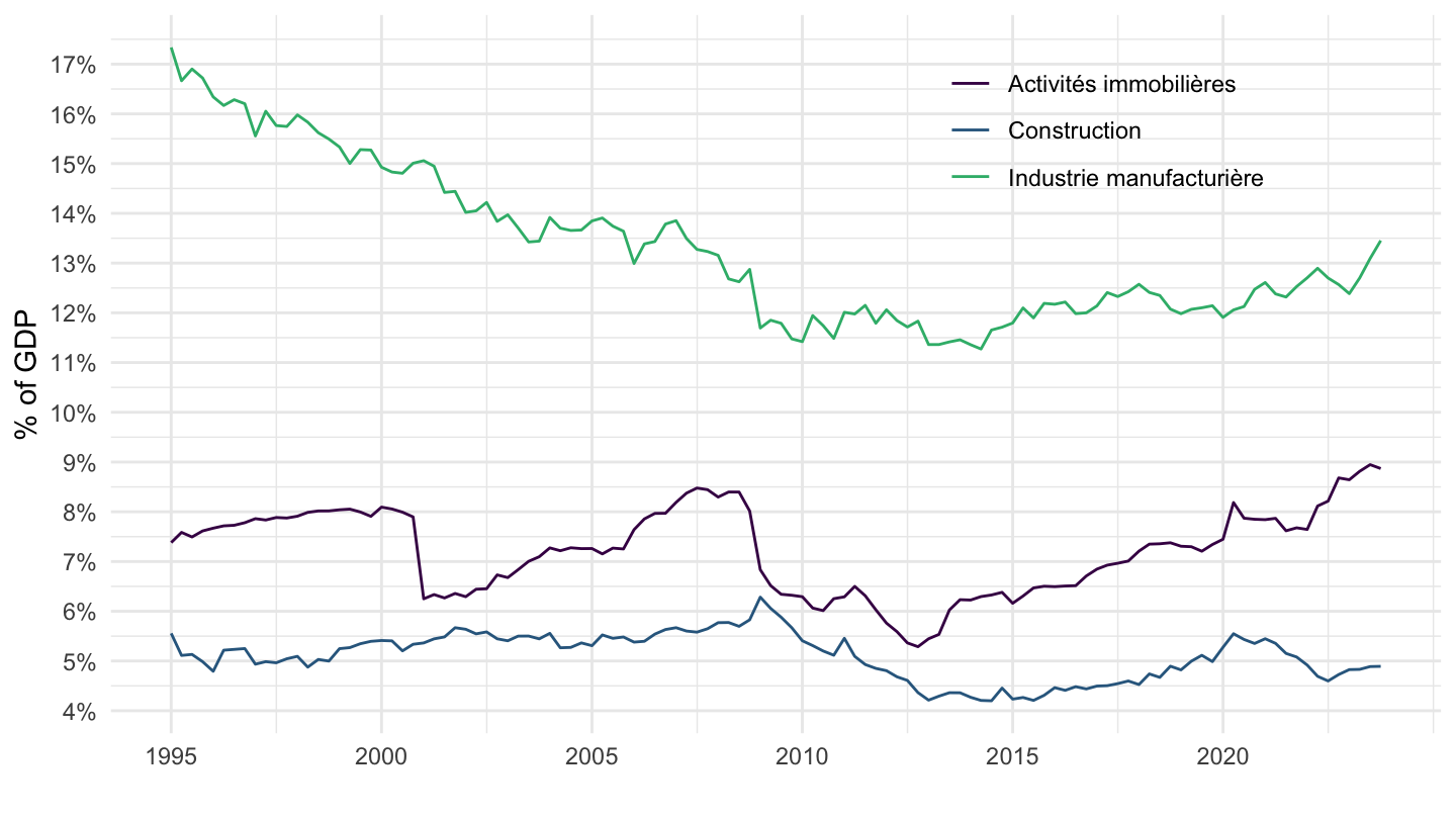
Danemark
Code
namq_10_a10 %>%
  filter(na_item == "B1G",
         nace_r2 %in% c("C", "TOTAL", "L", "Q", "F"),
         geo %in% c("DK"),
         unit == "CP_MNAC",
         s_adj == "SCA") %>%
  quarter_to_date() %>%

  select(nace_r2, Nace_r2, date, values) %>%
  group_by(date) %>%
  mutate(values = values/ values[nace_r2 == "TOTAL"]) %>%
  filter(nace_r2 != "TOTAL")  %>%
  ggplot(.) + geom_line(aes(x = date, y = values, color = Nace_r2)) +
  theme_minimal() + xlab("") + ylab("% of GDP") +
  scale_color_manual(values = viridis(4)[1:3]) +
  scale_x_date(breaks = seq(1960, 2100, 5) %>% paste0("-01-01") %>% as.Date,
               labels = date_format("%Y")) +
  scale_y_continuous(breaks = 0.01*seq(-500, 200, 1),
                     labels = percent_format(accuracy = 1)) +
  theme(legend.position = c(0.75, 0.85),
        legend.title = element_blank())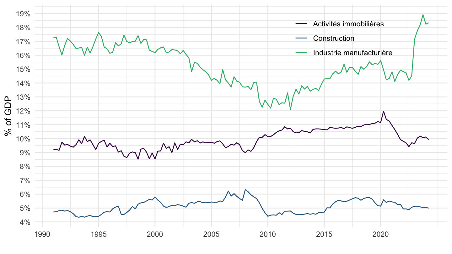
Belgium
Code
namq_10_a10 %>%
  filter(na_item == "B1G",
         nace_r2 %in% c("C", "TOTAL", "L", "Q", "F"),
         geo %in% c("BE"),
         unit == "CP_MNAC",
         s_adj == "SCA") %>%
  quarter_to_date() %>%

  select(nace_r2, Nace_r2, date, values) %>%
  group_by(date) %>%
  mutate(values = values/ values[nace_r2 == "TOTAL"]) %>%
  filter(nace_r2 != "TOTAL")  %>%
  ggplot(.) + geom_line(aes(x = date, y = values, color = Nace_r2)) +
  theme_minimal() + xlab("") + ylab("% of GDP") +
  scale_color_manual(values = viridis(4)[1:3]) +
  scale_x_date(breaks = seq(1960, 2100, 5) %>% paste0("-01-01") %>% as.Date,
               labels = date_format("%Y")) +
  scale_y_continuous(breaks = 0.01*seq(-500, 200, 1),
                     labels = percent_format(accuracy = 1)) +
  theme(legend.position = c(0.75, 0.85),
        legend.title = element_blank())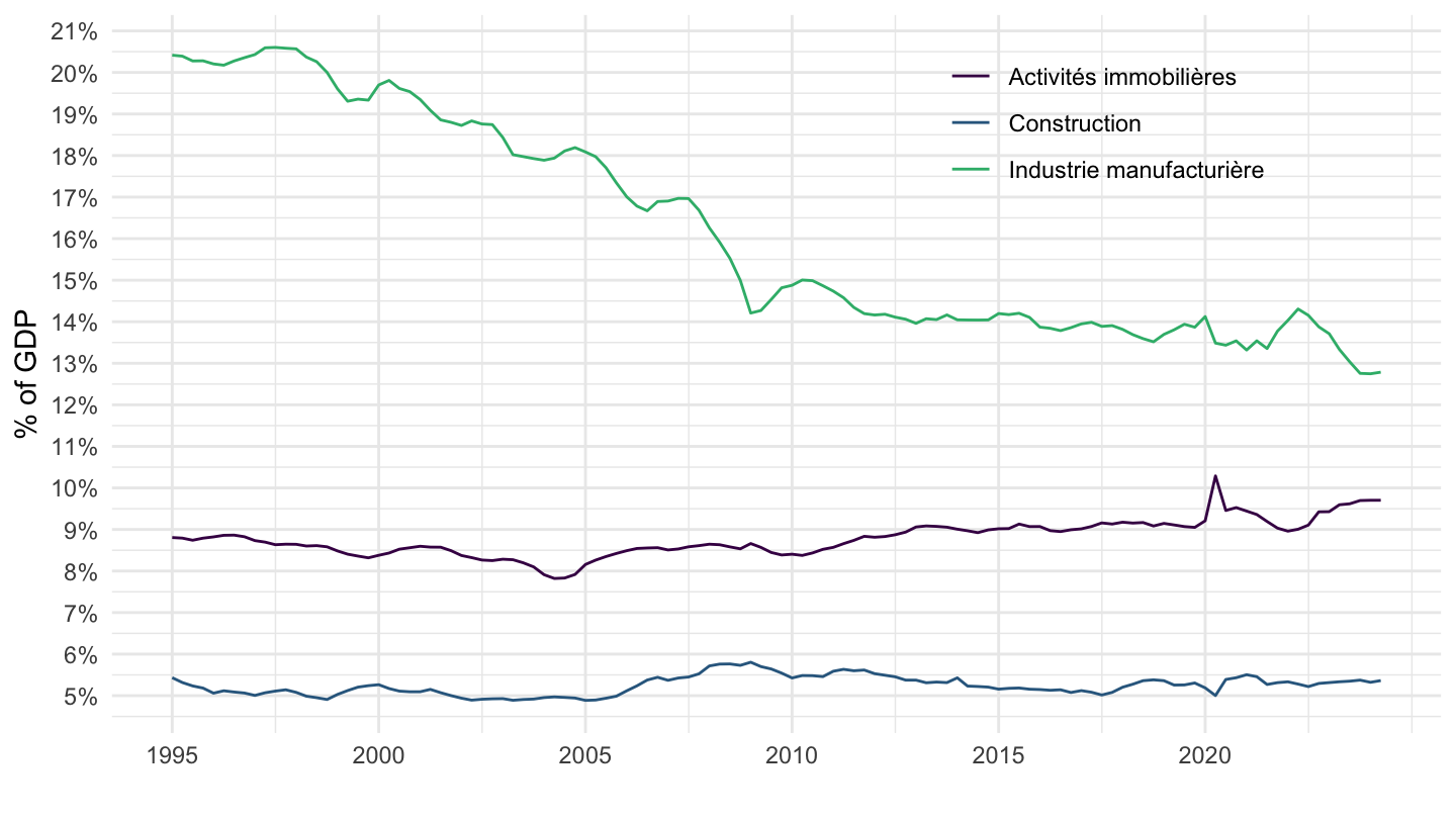
Finland
Code
namq_10_a10 %>%
  filter(na_item == "B1G",
         nace_r2 %in% c("C", "TOTAL", "L", "Q", "F"),
         geo %in% c("FI"),
         unit == "CP_MNAC",
         s_adj == "SCA") %>%
  quarter_to_date() %>%

  select(nace_r2, Nace_r2, date, values) %>%
  group_by(date) %>%
  mutate(values = values/ values[nace_r2 == "TOTAL"]) %>%
  filter(nace_r2 != "TOTAL")  %>%
  ggplot(.) + geom_line(aes(x = date, y = values, color = Nace_r2)) +
  theme_minimal() + xlab("") + ylab("% of GDP") +
  scale_color_manual(values = viridis(4)[1:3]) +
  scale_x_date(breaks = seq(1960, 2100, 5) %>% paste0("-01-01") %>% as.Date,
               labels = date_format("%Y")) +
  scale_y_continuous(breaks = 0.01*seq(-500, 200, 1),
                     labels = percent_format(accuracy = 1)) +
  theme(legend.position = c(0.75, 0.85),
        legend.title = element_blank())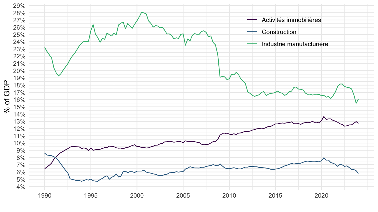
Portugal
Code
namq_10_a10 %>%
  filter(na_item == "B1G",
         nace_r2 %in% c("C", "TOTAL", "L", "Q", "F"),
         geo %in% c("PT"),
         unit == "CP_MNAC",
         s_adj == "SCA") %>%
  quarter_to_date() %>%

  select(nace_r2, Nace_r2, date, values) %>%
  group_by(date) %>%
  mutate(values = values/ values[nace_r2 == "TOTAL"]) %>%
  filter(nace_r2 != "TOTAL")  %>%
  ggplot(.) + geom_line(aes(x = date, y = values, color = Nace_r2)) +
  theme_minimal() + xlab("") + ylab("% of GDP") +
  scale_color_manual(values = viridis(4)[1:3]) +
  scale_x_date(breaks = seq(1960, 2100, 5) %>% paste0("-01-01") %>% as.Date,
               labels = date_format("%Y")) +
  scale_y_continuous(breaks = 0.01*seq(-500, 200, 1),
                     labels = percent_format(accuracy = 1)) +
  theme(legend.position = c(0.75, 0.85),
        legend.title = element_blank())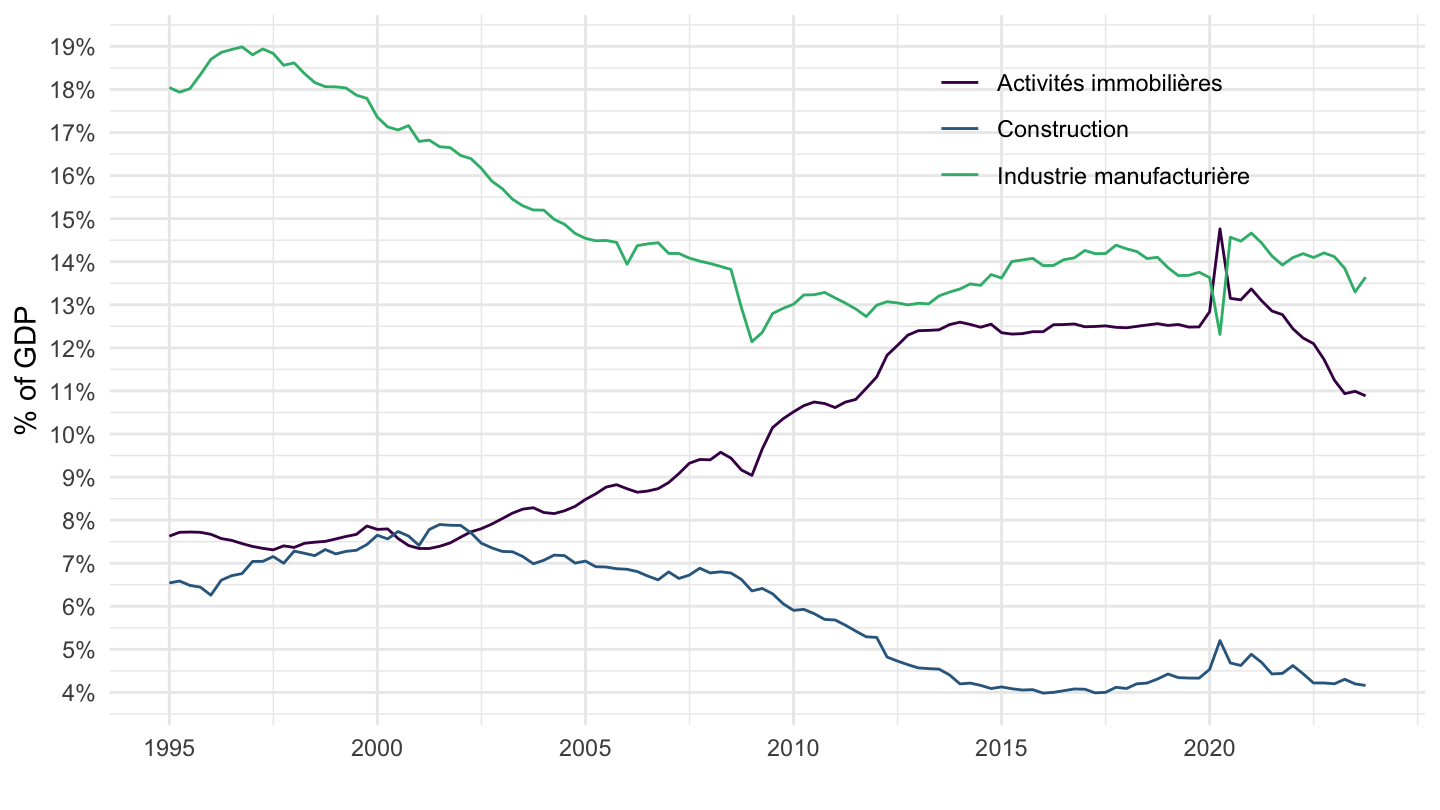
Austria
Code
namq_10_a10 %>%
  filter(na_item == "B1G",
         nace_r2 %in% c("C", "TOTAL", "L", "Q", "F"),
         geo %in% c("AT"),
         unit == "CP_MNAC",
         s_adj == "SCA") %>%
  quarter_to_date() %>%

  select(nace_r2, Nace_r2, date, values) %>%
  group_by(date) %>%
  mutate(values = values/ values[nace_r2 == "TOTAL"]) %>%
  filter(nace_r2 != "TOTAL")  %>%
  ggplot(.) + geom_line(aes(x = date, y = values, color = Nace_r2)) +
  theme_minimal() + xlab("") + ylab("% of GDP") +
  scale_color_manual(values = viridis(4)[1:3]) +
  scale_x_date(breaks = seq(1960, 2100, 5) %>% paste0("-01-01") %>% as.Date,
               labels = date_format("%Y")) +
  scale_y_continuous(breaks = 0.01*seq(-500, 200, 1),
                     labels = percent_format(accuracy = 1)) +
  theme(legend.position = c(0.75, 0.85),
        legend.title = element_blank())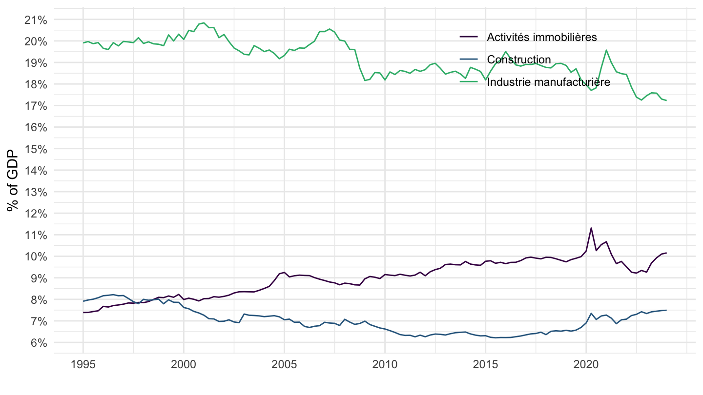
Sweden
Code
namq_10_a10 %>%
  filter(na_item == "B1G",
         nace_r2 %in% c("C", "TOTAL", "L", "Q", "F"),
         geo %in% c("SE"),
         unit == "CP_MNAC",
         s_adj == "SCA") %>%
  quarter_to_date() %>%

  select(nace_r2, Nace_r2, date, values) %>%
  group_by(date) %>%
  mutate(values = values/ values[nace_r2 == "TOTAL"]) %>%
  filter(nace_r2 != "TOTAL")  %>%
  ggplot(.) + geom_line(aes(x = date, y = values, color = Nace_r2)) +
  theme_minimal() + xlab("") + ylab("% of GDP") +
  scale_color_manual(values = viridis(4)[1:3]) +
  scale_x_date(breaks = seq(1960, 2100, 5) %>% paste0("-01-01") %>% as.Date,
               labels = date_format("%Y")) +
  scale_y_continuous(breaks = 0.01*seq(-500, 200, 1),
                     labels = percent_format(accuracy = 1)) +
  theme(legend.position = c(0.75, 0.85),
        legend.title = element_blank())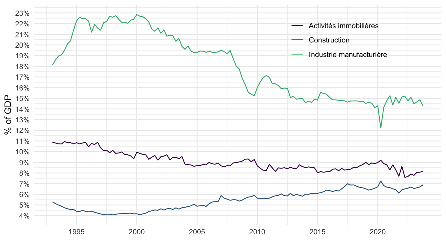
Relative to EA Manufacturing Value Added
1995-
NSA
Code
namq_10_a10 %>%
  filter(na_item == "B1G",
         nace_r2 == "C",
         geo %in% c("EA", "FR", "DE", "IT", "ES", "NL", "AT", "FI"),
         unit == "CP_MNAC",
         s_adj == "NSA") %>%
  quarter_to_date() %>%
  filter(date >= as.Date("1995-01-01")) %>%
  #filter(date <= as.Date("2019-01-01")) %>%

  group_by(date) %>%
  filter(n() == 8) %>%
  mutate(values = values /values[geo == "EA"]) %>%
  filter(geo != "EA") %>%
  group_by(geo) %>%
  mutate(values = 100*values / values[date == as.Date("1995-01-01")]) %>%
  left_join(colors, by = c("Geo" = "country")) %>%
  mutate(color = ifelse(geo == "FR", color2, color)) %>%
  ggplot(.) + geom_line(aes(x = date, y = values, color = color)) +
  theme_minimal() + xlab("") + ylab("Valeur ajoutée manuf. par rapport à la Zone €") +
  scale_color_identity() + add_flags +
  scale_x_date(breaks = seq(1960, 2100, 5) %>% paste0("-01-01") %>% as.Date,
               labels = date_format("%Y")) +
  scale_y_continuous(breaks = seq(0, 200, 5)) +
  theme(legend.position = "none")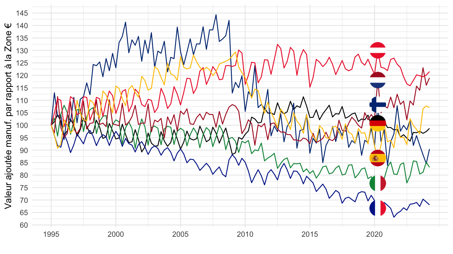
SCA
Code
namq_10_a10 %>%
  filter(na_item == "B1G",
         nace_r2 == "C",
         geo %in% c("EA", "FR", "DE", "IT", "ES", "NL", "AT", "FI"),
         unit == "CP_MNAC",
         s_adj == "SCA") %>%
  quarter_to_date() %>%
  filter(date >= as.Date("1995-01-01")) %>%
  #filter(date <= as.Date("2019-01-01")) %>%

  group_by(date) %>%
  filter(n() == 8) %>%
  mutate(values = values /values[geo == "EA"]) %>%
  filter(geo != "EA") %>%
  group_by(geo) %>%
  mutate(values = 100*values / values[date == as.Date("1995-01-01")]) %>%
  left_join(colors, by = c("Geo" = "country")) %>%
  mutate(color = ifelse(geo == "FR", color2, color)) %>%
  ggplot(.) + geom_line(aes(x = date, y = values, color = color)) +
  theme_minimal() + xlab("") + ylab("Valeur ajoutée manuf. par rapport à la Zone €") +
  scale_color_identity() + add_flags +
  scale_x_date(breaks = seq(1960, 2100, 5) %>% paste0("-01-01") %>% as.Date,
               labels = date_format("%Y")) +
  scale_y_continuous(breaks = seq(0, 200, 5)) +
  theme(legend.position = "none")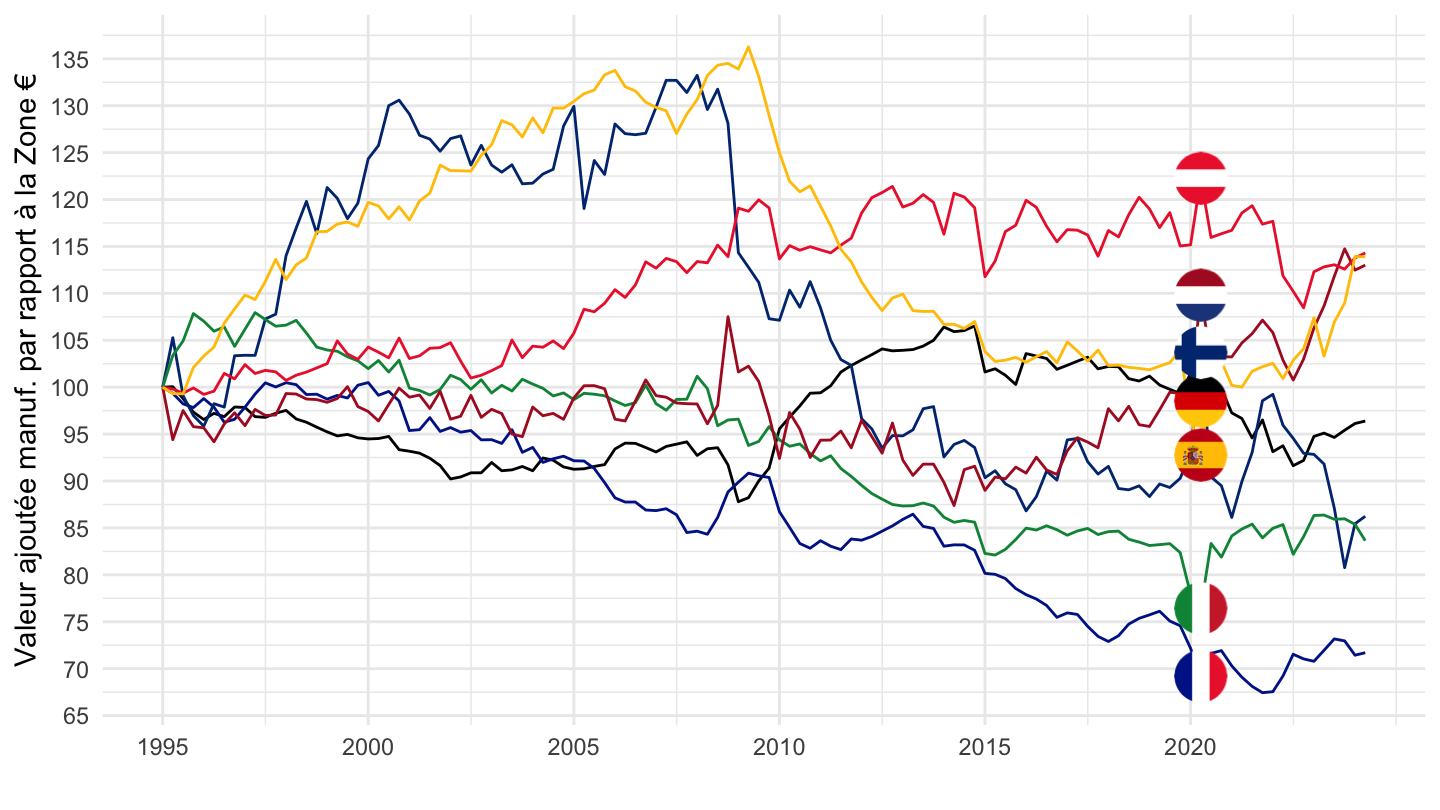
SCA
Code
namq_10_a10 %>%
  filter(na_item == "B1G",
         nace_r2 == "C",
         geo %in% c("EA", "FR", "DE", "IT", "ES", "NL"),
         unit == "CP_MNAC",
         s_adj == "SCA") %>%
  quarter_to_date() %>%
  filter(date >= as.Date("1995-01-01")) %>%
  #filter(date <= as.Date("2019-01-01")) %>%

  group_by(date) %>%
  filter(n() == 6) %>%
  mutate(values = values /values[geo == "EA"]) %>%
  filter(geo != "EA") %>%
  group_by(geo) %>%
  mutate(values = 100*values / values[date == as.Date("1995-01-01")]) %>%
  left_join(colors, by = c("Geo" = "country")) %>%
  mutate(color = ifelse(geo == "FR", color2, color)) %>%
  ggplot(.) + geom_line(aes(x = date, y = values, color = color)) +
  theme_minimal() + xlab("") + ylab("Valeur ajoutée manuf. par rapport à la Zone €") +
  scale_color_identity() + add_flags +
  scale_x_date(breaks = seq(1960, 2100, 2) %>% paste0("-01-01") %>% as.Date,
               labels = date_format("%Y")) +
  scale_y_continuous(breaks = seq(0, 200, 5)) +
  theme(legend.position = "none")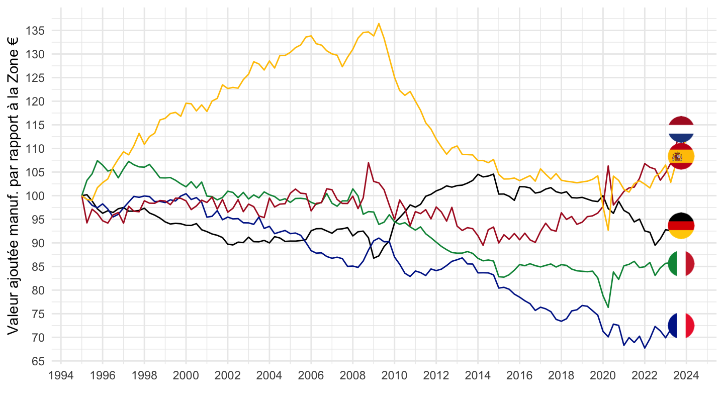
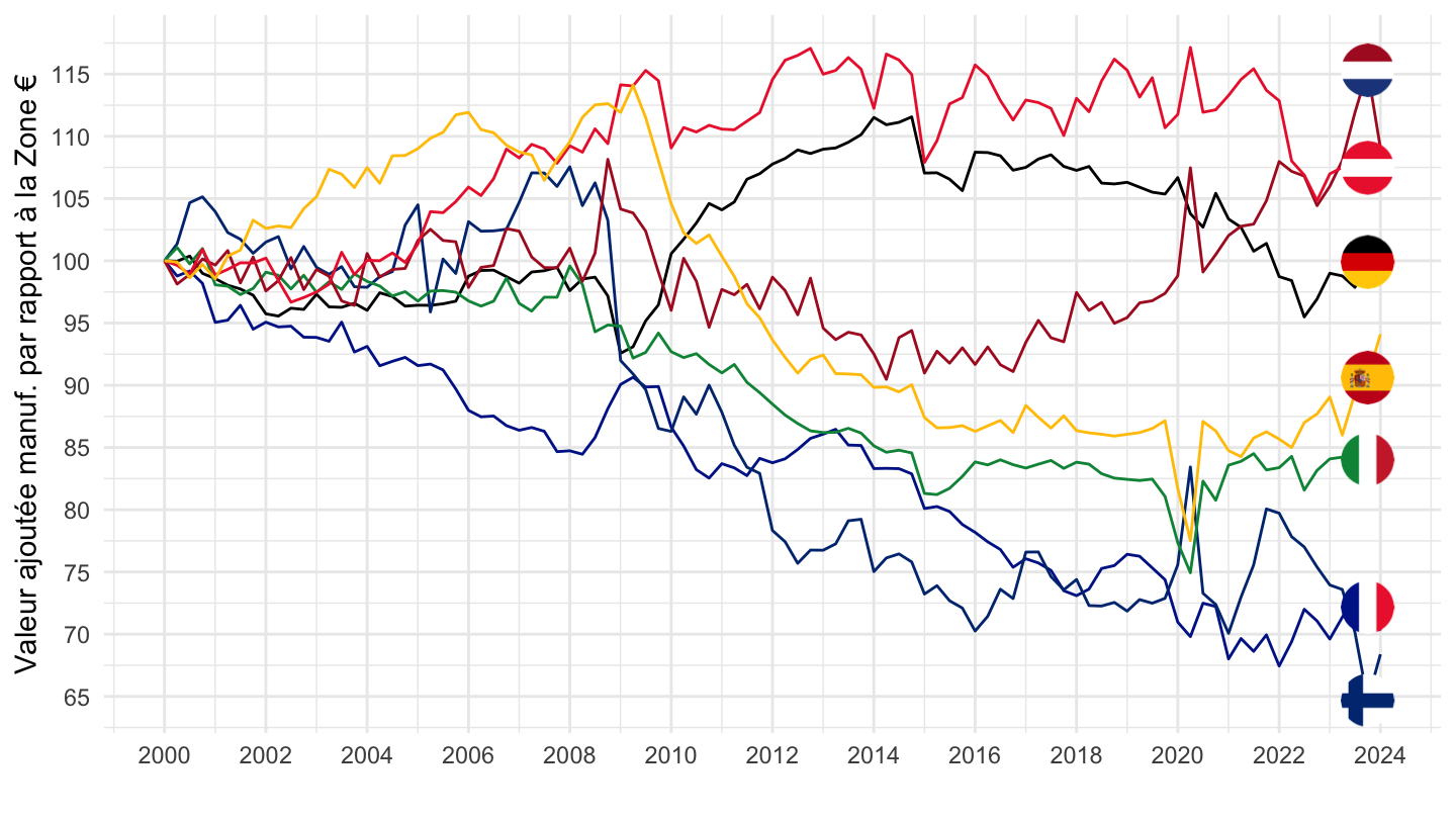
2000-
Code
namq_10_a10 %>%
  filter(na_item == "B1G",
         nace_r2 == "C",
         geo %in% c("EA", "FR", "DE", "IT", "ES", "NL", "AT", "FI"),
         unit == "CP_MNAC",
         s_adj == "SCA") %>%
  quarter_to_date() %>%
  filter(date >= as.Date("2000-01-01")) %>%
  #filter(date <= as.Date("2019-01-01")) %>%

  group_by(date) %>%
  filter(n() == 8) %>%
  mutate(values = values /values[geo == "EA"]) %>%
  filter(geo != "EA") %>%
  group_by(geo) %>%
  mutate(values = 100*values / values[date == as.Date("2000-01-01")]) %>%
  left_join(colors, by = c("Geo" = "country")) %>%
  mutate(color = ifelse(geo == "FR", color2, color)) %>%
  ggplot(.) + geom_line(aes(x = date, y = values, color = color)) +
  theme_minimal() + xlab("") + ylab("Valeur ajoutée manuf. par rapport à la Zone €") +
  scale_color_identity() + add_flags +
  scale_x_date(breaks = seq(1960, 2100, 2) %>% paste0("-01-01") %>% as.Date,
               labels = date_format("%Y")) +
  scale_y_continuous(breaks = seq(0, 200, 5)) +
  theme(legend.position = "none")