Disposable income and net lending - net borrowing

Data - OECD

Author

Info

Related main macro datasets

source	dataset	Title	Download	Compile
oecd	SNA_TABLE2	Disposable income and net lending - net borrowing	2024-04-11	[2024-06-19]
eurostat	nama_10_a10	Gross value added and income by A*10 industry breakdowns	2024-06-08	[2024-06-20]
eurostat	nama_10_a10_e	Employment by A*10 industry breakdowns	2024-06-18	[2024-06-20]
eurostat	nama_10_gdp	GDP and main components (output, expenditure and income)	2024-06-18	[2024-06-20]
eurostat	nama_10_lp_ulc	Labour productivity and unit labour costs	2024-06-08	[2024-06-20]
eurostat	namq_10_a10	Gross value added and income A*10 industry breakdowns	2024-06-18	[2024-06-20]
eurostat	namq_10_a10_e	Employment A*10 industry breakdowns	2024-06-08	[2024-06-20]
eurostat	namq_10_gdp	GDP and main components (output, expenditure and income)	2024-06-08	[2024-06-20]
eurostat	namq_10_lp_ulc	Labour productivity and unit labour costs	2024-06-08	[2024-06-20]
eurostat	namq_10_pc	Main GDP aggregates per capita	2024-06-18	[2024-06-20]
eurostat	nasa_10_nf_tr	Non-financial transactions	2024-06-08	[2024-06-20]
eurostat	nasq_10_nf_tr	Non-financial transactions	2024-06-08	[2024-06-20]
fred	gdp	Gross Domestic Product	2024-06-07	[2024-06-20]
oecd	QNA	Quarterly National Accounts, Per Capita	2024-06-05	[2024-06-06]
oecd	SNA_TABLE1	Gross domestic product (GDP)	2024-06-01	[2024-06-20]
oecd	SNA_TABLE14A	Non-financial accounts by sectors	2024-04-15	[2024-06-20]
oecd	SNA_TABLE6A	Value added and its components by activity, ISIC rev4	2024-04-15	[2024-06-19]
wdi	NE.RSB.GNFS.ZS	External balance on goods and services (% of GDP)	2024-04-14	[2024-06-20]
wdi	NY.GDP.MKTP.CD	GDP (current USD)	2024-05-06	[2024-06-20]
wdi	NY.GDP.MKTP.PP.CD	GDP, PPP (current international D)	2024-04-14	[2024-06-20]
wdi	NY.GDP.PCAP.CD	GDP per capita (current USD)	2024-04-22	[2024-06-20]
wdi	NY.GDP.PCAP.KD	GDP per capita (constant 2015 USD)	2024-05-06	[2024-06-20]
wdi	NY.GDP.PCAP.PP.CD	GDP per capita, PPP (current international D)	2024-04-22	[2024-06-20]
wdi	NY.GDP.PCAP.PP.KD	GDP per capita, PPP (constant 2011 international D)	2024-05-06	[2024-06-20]

LAST_COMPILE

COMPILE_TIME
2024-06-20

Last

obsTime	Nobs
2023	15

Layout

OECD Website. html

TRANSACT

Code

SNA_TABLE2 %>%
  left_join(SNA_TABLE2_var$TRANSACT, by = "TRANSACT") %>%
  group_by(TRANSACT, Transact) %>%
  summarise(Nobs = n()) %>%
  arrange(-Nobs) %>%
  print_table_conditional()

TRANSACT	Transact	Nobs
B1_GS1	Gross domestic product	24088
B5_GS1	Gross national income at market prices	18208
B5_NS1	Net national income at market prices	18008
GDIS1	Gross domestic income	16179
B6NS1	Net national disposable income	14847
B6GS1	Gross national disposable income	14617
D5_D7NFRS2	Net current transfers from the rest of the world	14520
D1_D4NFRS2	Net primary incomes from the rest of the world	14388
D1_D4TOS2	Primary incomes payable to the rest of the world	14309
D5_D7TOS2	Current transfers payable to the rest of the world	14075
D5_D7FRS2	Current transfers receivable from the rest of the world	13953
D1_D4FRS2	Primary incomes receivable from the rest of the world	13879
K1MS1	Consumption of fixed capital	12180
P3S1	Final consumption expenditures	10434
P5S1	Gross capital formation	10389
B8NS1	Saving, net	9456
B9S1	Net lending/net borrowing	9437
K1S1	Consumption of fixed capital, capital account	9015
D9TOS2	Capital transfers payable to the rest of the world	8602
D9NFRS2	Net capital transfers from the rest of the world	8521
D9FRS2	Capital transfers receivable from the rest of the world	8186
K2S1	Acquisitions less disposals of non-financial non-produced assets	7206
D8S1	Adjustment for the change in net equity of households in pension funds	6373
TGLS1	Trading gain or loss	3956
B1_GE	Gross domestic product (expenditure approach)	2771

MEASURE

Code

SNA_TABLE2 %>%
  left_join(SNA_TABLE2_var$MEASURE, by = "MEASURE") %>%
  group_by(MEASURE, Measure) %>%
  summarise(Nobs = n()) %>%
  print_table_conditional()

MEASURE	Measure	Nobs
C	Current prices	45273
CPC	Current prices, current PPPs	42245
CXC	Current prices, current exchange rates	42958
HCPC	Per head, current prices, current PPPs	3815
HVPVOB	Per head, constant prices, constant PPPs, OECD base year	1279
PVP	Previous year prices and previous year PPPs	1868
V	Constant prices, national base year	17657
VOB	Constant prices, OECD base year	18320
VP	Constant prices, previous year prices	552
VPCOB	Current prices, constant PPPs, OECD base year	42479
VPVOB	Constant prices, constant PPPs, OECD base year	18375
VXCOB	Current prices, constant exchange rates, OECD base year	42479
VXVOB	Constant prices, constant exchange rates, OECD base year	18375
XVP	Previous year prices and previous year exchange rates	1922

LOCATION

Code

SNA_TABLE2 %>%
  left_join(SNA_TABLE2_var$LOCATION, by = "LOCATION") %>%
  group_by(LOCATION, Location) %>%
  summarise(Nobs = n()) %>%
  arrange(-Nobs) %>%
  mutate(Flag = gsub(" ", "-", str_to_lower(gsub(" ", "-", Location))),
         Flag = paste0('<img src="../../icon/flag/vsmall/', Flag, '.png" alt="Flag">')) %>%
  select(Flag, everything()) %>%
  {if (is_html_output()) datatable(., filter = 'top', rownames = F, escape = F) else .}

B1_GE - Gross domestic product

All Decomposition

Code

SNA_TABLE2 %>%
  filter(LOCATION %in% c("FRA", "DEU", "USA", "GBR"),
         obsTime == "2018",
         MEASURE == "C") %>%
  select(LOCATION, TRANSACT, obsValue) %>%
  left_join(SNA_TABLE2_var$TRANSACT %>%
              setNames(c("TRANSACT", "Transact")), by = "TRANSACT") %>%
  spread(LOCATION, obsValue) %>%
  mutate_at(vars(-1, -2), funs(ifelse(is.na(.), "", paste0(round(100*./.[TRANSACT == "B1_GE"], 1), " %")))) %>%
  {if (is_html_output()) datatable(., filter = 'top', rownames = F) else .}

How much data

Code

SNA_TABLE2 %>%
  filter(TRANSACT == "B1_GE",
         MEASURE == "C") %>%
  left_join(SNA_TABLE2_var$LOCATION %>%
              setNames(c("LOCATION", "Location")), 
            by = "LOCATION") %>%
  group_by(LOCATION, UNIT, Location) %>%
  summarise(year_first = first(obsTime),
            year_last = last(obsTime),
            value_last = last(round(obsValue))) %>%
  mutate(Loc = gsub(" ", "-", str_to_lower(Location)),
         Loc = paste0('<img src="../../bib/flags/vsmall/', Loc, '.png" alt="Flag">')) %>%
  select(Loc, everything()) %>%
  {if (is_html_output()) datatable(., filter = 'top', rownames = F, escape = F) else .}

All

US and France

Code

SNA_TABLE2 %>%
  filter(obsTime == "2018",
         MEASURE == "C",
         LOCATION %in% c("USA", "FRA")) %>%
  select(LOCATION, TRANSACT, obsValue) %>%
  left_join(SNA_TABLE2_var$TRANSACT %>%
              setNames(c("TRANSACT", "Transact")), by = "TRANSACT") %>%
  spread(LOCATION, obsValue) %>%
  mutate_at(vars(-1, -2), funs(ifelse(is.na(.), "", paste0(round(100*./.[TRANSACT == "B1_GE"], 1), " %")))) %>%
  {if (is_html_output()) print_table(.) else .}

TRANSACT	Transact	FRA	USA
B1_GE	Gross domestic product (expenditure approach)	100 %	100 %
B1_GS1	Gross domestic product	100 %	100 %
B5_GS1	Gross national income at market prices	102.3 %	101.1 %
B5_NS1	Net national income at market prices	84.1 %	85.1 %
B6GS1	Gross national disposable income	100.3 %	100.4 %
B6NS1	Net national disposable income	82.1 %	84.4 %
B8NS1	Saving, net	5 %	3.1 %
B9S1	Net lending/net borrowing	-0.7 %	-2.5 %
D1_D4FRS2	Primary incomes receivable from the rest of the world	7.6 %	5.5 %
D1_D4NFRS2	Net primary incomes from the rest of the world	2.3 %	1.4 %
D1_D4TOS2	Primary incomes payable to the rest of the world	5.3 %	4.1 %
D5_D7FRS2	Current transfers receivable from the rest of the world	1.1 %	0.7 %
D5_D7NFRS2	Net current transfers from the rest of the world	-2 %	-0.7 %
D5_D7TOS2	Current transfers payable to the rest of the world	3.1 %	1.4 %
D8S1	Adjustment for the change in net equity of households in pension funds	0 %	0 %
D9FRS2	Capital transfers receivable from the rest of the world	0.1 %	0 %
D9NFRS2	Net capital transfers from the rest of the world	0 %	0 %
D9TOS2	Capital transfers payable to the rest of the world	0 %	0 %
GDIS1	Gross domestic income	100 %	100.6 %
K1MS1	Consumption of fixed capital	18.2 %	16 %
K1S1	Consumption of fixed capital, capital account	18.2 %	16 %
K2S1	Acquisitions less disposals of non-financial non-produced assets	0 %	0 %
P3S1	Final consumption expenditures	77.2 %	81.3 %
P5S1	Gross capital formation	23.9 %	21.6 %

B6GS1 - Gross National Disposable Income / GDP

France, Germany, Italy

Code

SNA_TABLE2 %>%
  filter(MEASURE == "C",
         LOCATION %in% c("FRA", "DEU", "ITA"),
         TRANSACT %in% c("B1_GE", "B6GS1")) %>%
  year_to_date %>%
  left_join(SNA_TABLE2_var$LOCATION, by = "LOCATION") %>%
  select(Location, date, TRANSACT, obsValue) %>%
  spread(TRANSACT, obsValue) %>%
  group_by(Location) %>%
  mutate(obsValue = B6GS1 / B1_GE) %>%
  select(Location, date, obsValue) %>%
  na.omit %>%
  left_join(colors, by = c("Location" = "country")) %>%
  ggplot() + geom_line(aes(x = date, y = obsValue, color = color)) +
  scale_color_identity() + theme_minimal() + add_3flags +
  scale_x_date(breaks = seq(1920, 2025, 10) %>% paste0("-01-01") %>% as.Date,
               labels = date_format("%Y")) +
  scale_y_continuous(breaks = 0.01*seq(-10, 200, 1),
                     labels = scales::percent_format(accuracy = 1)) +
  ylab("Gross National Disposable Income (% of GDP)") + xlab("")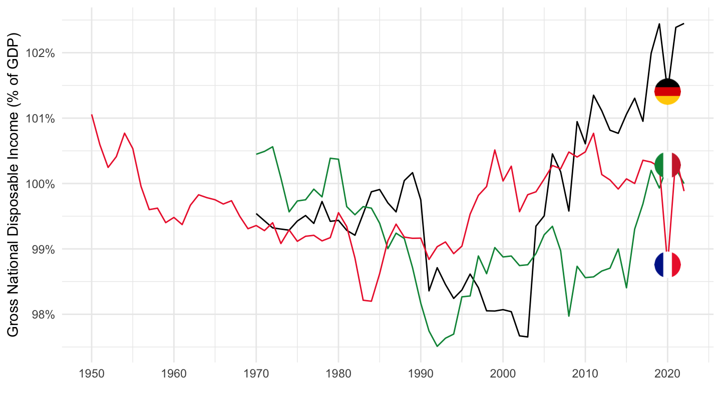

France, Germany, Belgium, Spain, Netherlands, Italy

All

Code

SNA_TABLE2 %>%
  filter(MEASURE == "C",
         LOCATION %in% c("FRA", "DEU", "BEL", "ESP", "NLD", "ITA"),
         TRANSACT %in% c("B1_GE", "B6GS1")) %>%
  year_to_date %>%
  left_join(SNA_TABLE2_var$LOCATION, by = "LOCATION") %>%
  select(Location, date, TRANSACT, obsValue) %>%
  spread(TRANSACT, obsValue) %>%
  group_by(Location) %>%
  mutate(obsValue = B6GS1 / B1_GE) %>%
  select(Location, date, obsValue) %>%
  na.omit %>%
  left_join(colors, by = c("Location" = "country")) %>%
  mutate(color = ifelse(Location == "Netherlands", color2, color)) %>%
  ggplot() + geom_line(aes(x = date, y = obsValue, color = color)) +
  scale_color_identity() + theme_minimal() + add_6flags +
  scale_x_date(breaks = seq(1920, 2025, 10) %>% paste0("-01-01") %>% as.Date,
               labels = date_format("%Y")) +
  scale_y_continuous(breaks = 0.01*seq(-10, 100, 1),
                     labels = scales::percent_format(accuracy = 1)) +
  ylab("Gross National Disposable Income (% of GDP)") + xlab("")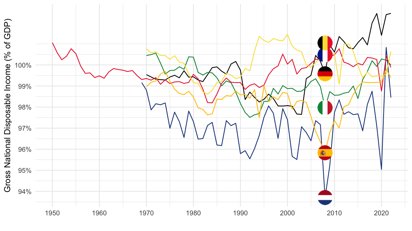

1995-

Code

SNA_TABLE2 %>%
  filter(MEASURE == "C",
         LOCATION %in% c("FRA", "DEU", "BEL", "ESP", "NLD", "ITA"),
         TRANSACT %in% c("B1_GE", "B6GS1")) %>%
  year_to_date %>%
  left_join(SNA_TABLE2_var$LOCATION, by = "LOCATION") %>%
  select(Location, date, TRANSACT, obsValue) %>%
  spread(TRANSACT, obsValue) %>%
  group_by(Location) %>%
  mutate(obsValue = B6GS1 / B1_GE) %>%
  select(Location, date, obsValue) %>%
  na.omit %>%
  left_join(colors, by = c("Location" = "country")) %>%
  mutate(color = ifelse(Location == "Netherlands", color2, color)) %>%
  filter(date >= as.Date("1995-01-01")) %>%
  ggplot() + geom_line(aes(x = date, y = obsValue, color = color)) +
  scale_color_identity() + theme_minimal() + add_6flags +
  scale_x_date(breaks = seq(1920, 2025, 5) %>% paste0("-01-01") %>% as.Date,
               labels = date_format("%Y")) +
  scale_y_continuous(breaks = 0.01*seq(-10, 120, 1),
                     labels = scales::percent_format(accuracy = 1)) +
  ylab("Gross National Disposable Income (% of GDP)") + xlab("")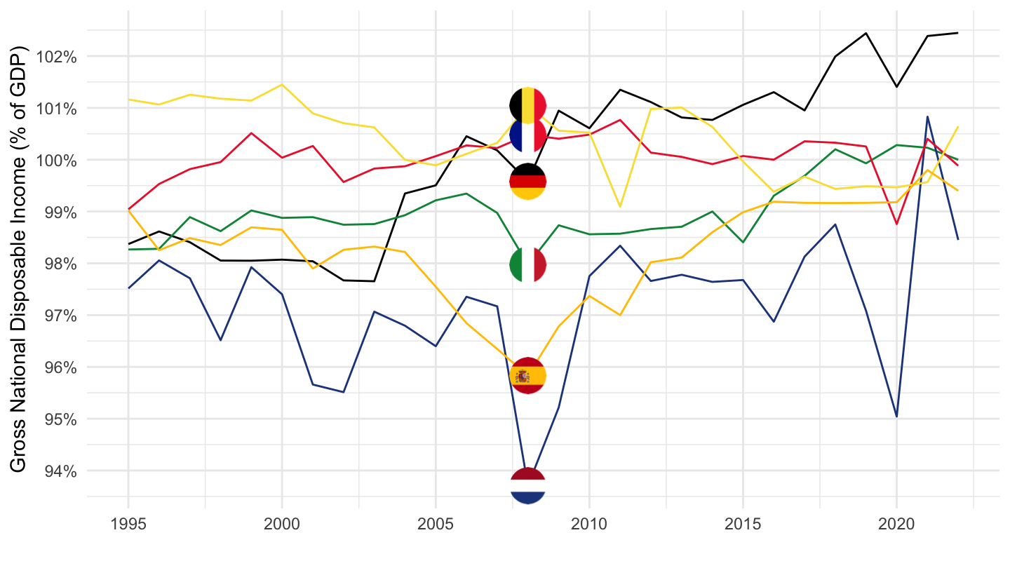

B6NS1 - Net national disposable income / GDP

France, Germany, Italy

Code

SNA_TABLE2 %>%
  filter(MEASURE == "C",
         LOCATION %in% c("FRA", "DEU", "ITA"),
         TRANSACT %in% c("B1_GE", "B6NS1")) %>%
  year_to_date %>%
  left_join(SNA_TABLE2_var$LOCATION, by = "LOCATION") %>%
  select(Location, date, TRANSACT, obsValue) %>%
  spread(TRANSACT, obsValue) %>%
  group_by(Location) %>%
  mutate(obsValue = B6NS1 / B1_GE) %>%
  select(Location, date, obsValue) %>%
  na.omit %>%
  left_join(colors, by = c("Location" = "country")) %>%
  ggplot() + geom_line(aes(x = date, y = obsValue, color = color)) +
  scale_color_identity() + theme_minimal() + add_3flags +
  scale_x_date(breaks = seq(1920, 2025, 10) %>% paste0("-01-01") %>% as.Date,
               labels = date_format("%Y")) +
  scale_y_continuous(breaks = 0.01*seq(-10, 100, 1),
                     labels = scales::percent_format(accuracy = 1)) +
  ylab("Net National Disposable Income (% of GDP)") + xlab("")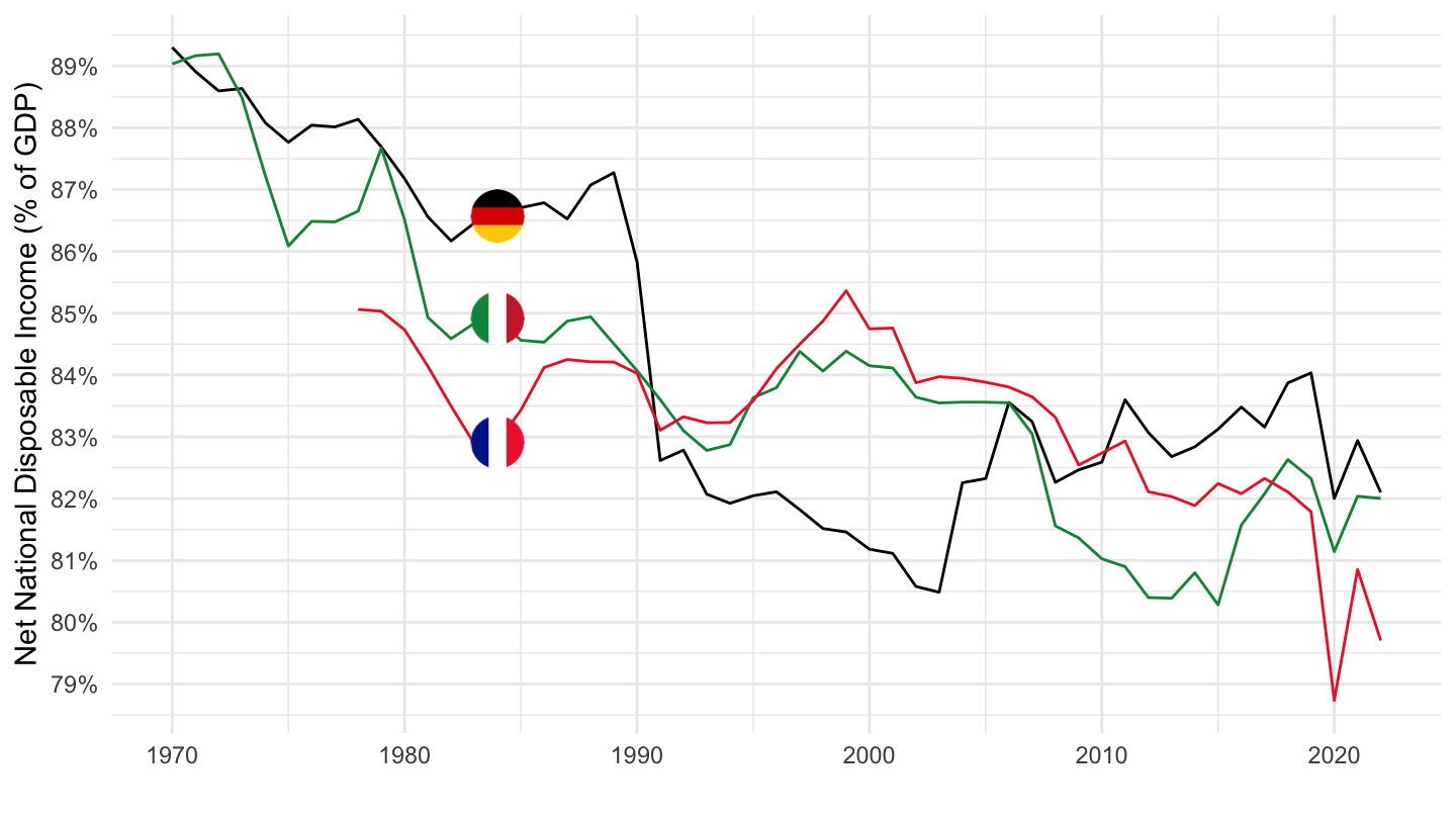

France, Germany, US, Denmark

Code

SNA_TABLE2 %>%
  filter(MEASURE == "C",
         LOCATION %in% c("FRA", "DEU", "DNK", "USA"),
         TRANSACT %in% c("B1_GE", "B6NS1")) %>%
  year_to_date %>%
  left_join(SNA_TABLE2_var$LOCATION, by = "LOCATION") %>%
  select(LOCATION, Location, date, TRANSACT, obsValue) %>%
  spread(TRANSACT, obsValue) %>%
  group_by(Location) %>%
  mutate(obsValue = B6NS1 / B1_GE) %>%
  select(LOCATION, Location, date, obsValue) %>%
  na.omit %>%
  left_join(colors, by = c("Location" = "country")) %>%
  mutate(color = ifelse(LOCATION == "FRA", color2, color)) %>%
  ggplot() + geom_line(aes(x = date, y = obsValue, color = color)) +
  scale_color_identity() + theme_minimal() + add_4flags +
  scale_x_date(breaks = seq(1920, 2025, 10) %>% paste0("-01-01") %>% as.Date,
               labels = date_format("%Y")) +
  scale_y_continuous(breaks = 0.01*seq(-10, 100, 1),
                     labels = scales::percent_format(accuracy = 1)) +
  ylab("Net National Disposable Income (% of GDP)") + xlab("")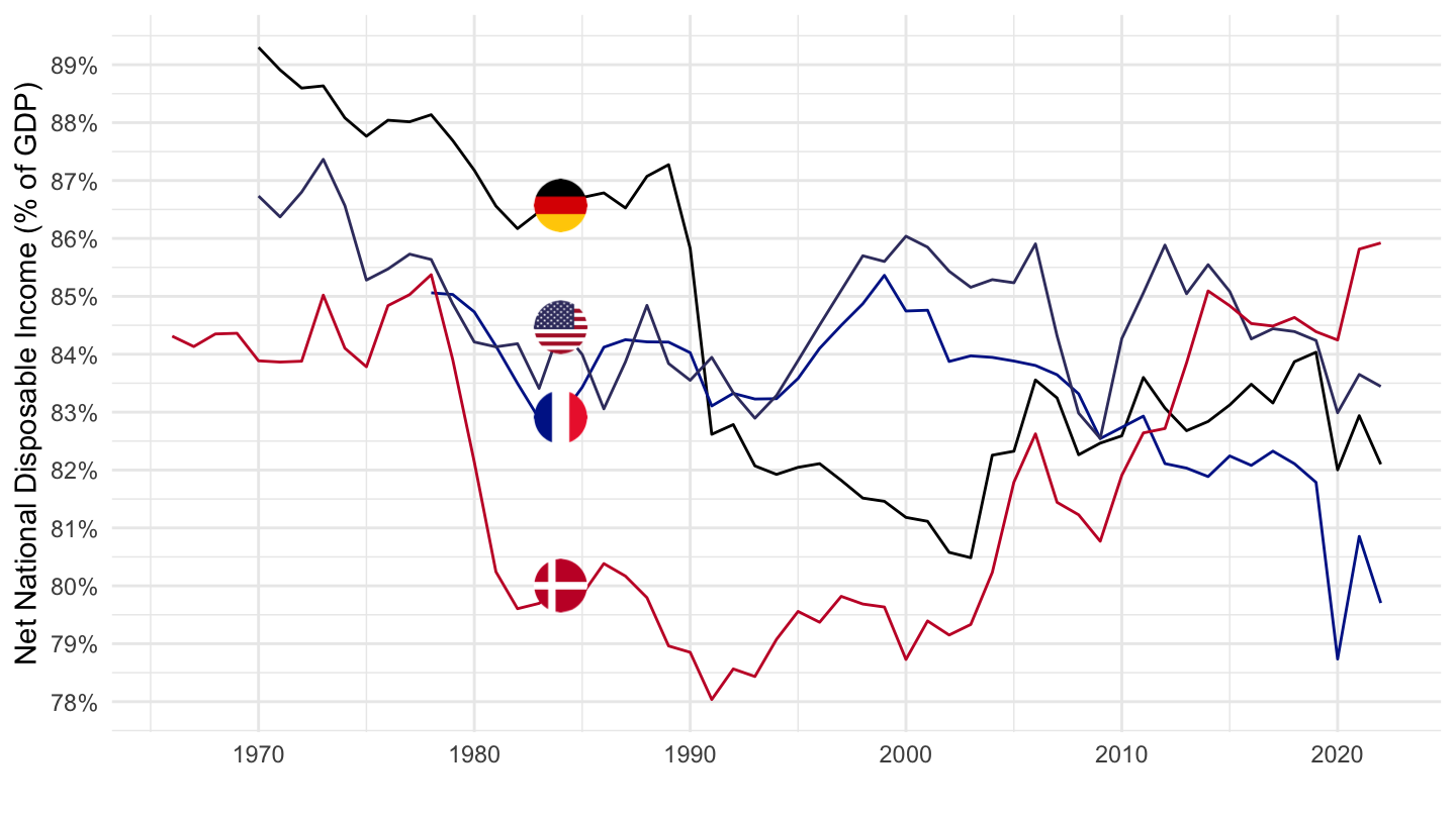

France, Germany, Belgium, Spain, Netherlands, Italy

All

Code

SNA_TABLE2 %>%
  filter(MEASURE == "C",
         LOCATION %in% c("FRA", "DEU", "BEL", "ESP", "NLD", "ITA"),
         TRANSACT %in% c("B1_GE", "B6NS1")) %>%
  year_to_date %>%
  left_join(SNA_TABLE2_var$LOCATION, by = "LOCATION") %>%
  select(Location, date, TRANSACT, obsValue) %>%
  spread(TRANSACT, obsValue) %>%
  group_by(Location) %>%
  mutate(obsValue = B6NS1 / B1_GE) %>%
  select(Location, date, obsValue) %>%
  na.omit %>%
  left_join(colors, by = c("Location" = "country")) %>%
  mutate(color = ifelse(Location == "Netherlands", color2, color)) %>%
  ggplot() + geom_line(aes(x = date, y = obsValue, color = color)) +
  scale_color_identity() + theme_minimal() + add_6flags +
  scale_x_date(breaks = seq(1920, 2025, 10) %>% paste0("-01-01") %>% as.Date,
               labels = date_format("%Y")) +
  scale_y_continuous(breaks = 0.01*seq(-10, 100, 1),
                     labels = scales::percent_format(accuracy = 1)) +
  ylab("Net National Disposable Income (% of GDP)") + xlab("")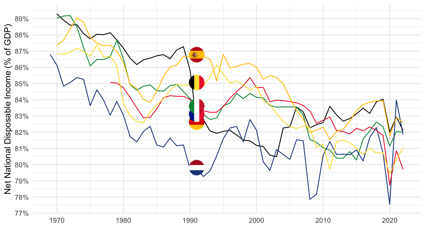

1995-

Code

SNA_TABLE2 %>%
  filter(MEASURE == "C",
         LOCATION %in% c("FRA", "DEU", "BEL", "ESP", "NLD", "ITA"),
         TRANSACT %in% c("B1_GE", "B6NS1")) %>%
  year_to_date %>%
  left_join(SNA_TABLE2_var$LOCATION, by = "LOCATION") %>%
  select(Location, date, TRANSACT, obsValue) %>%
  spread(TRANSACT, obsValue) %>%
  group_by(Location) %>%
  mutate(obsValue = B6NS1 / B1_GE) %>%
  select(Location, date, obsValue) %>%
  na.omit %>%
  left_join(colors, by = c("Location" = "country")) %>%
  mutate(color = ifelse(Location == "Netherlands", color2, color)) %>%
  filter(date >= as.Date("1995-01-01")) %>%
  ggplot() + geom_line(aes(x = date, y = obsValue, color = color)) +
  scale_color_identity() + theme_minimal() + add_6flags +
  scale_x_date(breaks = seq(1920, 2025, 5) %>% paste0("-01-01") %>% as.Date,
               labels = date_format("%Y")) +
  scale_y_continuous(breaks = 0.01*seq(-10, 100, 1),
                     labels = scales::percent_format(accuracy = 1)) +
  ylab("Net National Disposable Income (% of GDP)") + xlab("")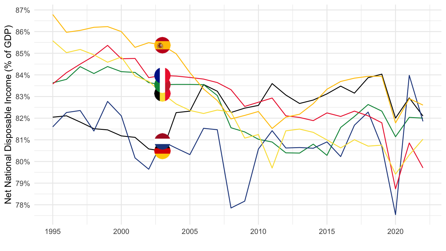

B8NS1 - Net Saving / GDP

France, Germany, Italy

Code

SNA_TABLE2 %>%
  filter(MEASURE == "C",
         LOCATION %in% c("FRA", "DEU", "ITA"),
         TRANSACT %in% c("B1_GE", "B8NS1")) %>%
  year_to_date %>%
  left_join(SNA_TABLE2_var$LOCATION, by = "LOCATION") %>%
  select(Location, date, TRANSACT, obsValue) %>%
  spread(TRANSACT, obsValue) %>%
  group_by(Location) %>%
  mutate(obsValue = B8NS1 / B1_GE) %>%
  select(Location, date, obsValue) %>%
  na.omit %>%
  left_join(colors, by = c("Location" = "country")) %>%
  ggplot() + geom_line(aes(x = date, y = obsValue, color = color)) +
  scale_color_identity() + theme_minimal() + add_3flags +
  scale_x_date(breaks = seq(1920, 2025, 10) %>% paste0("-01-01") %>% as.Date,
               labels = date_format("%Y")) +
  scale_y_continuous(breaks = 0.01*seq(-10, 100, 1),
                     labels = scales::percent_format(accuracy = 1)) +
  ylab("Net Saving (% of GDP)") + xlab("")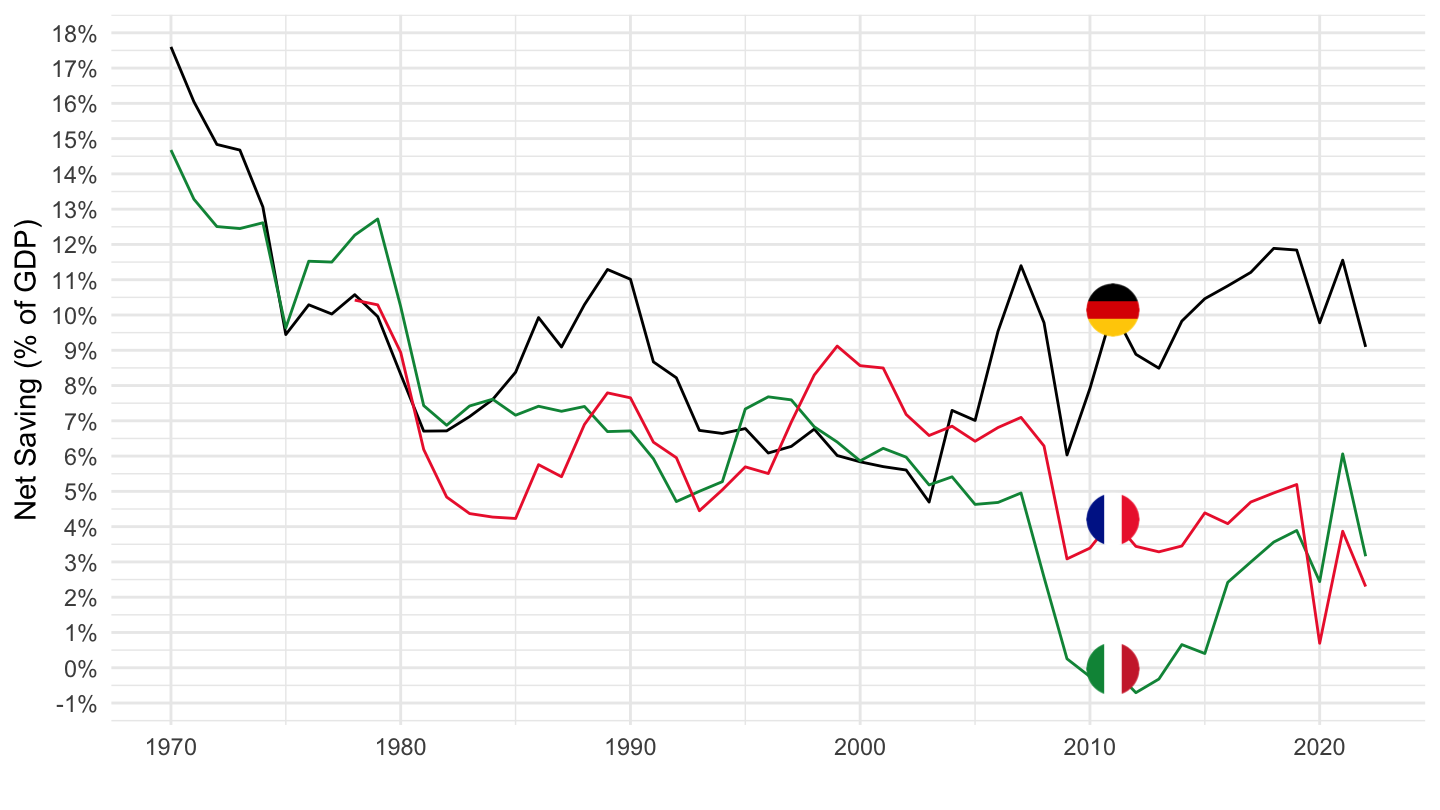

France, Italy

Code

SNA_TABLE2 %>%
  filter(MEASURE == "C",
         LOCATION %in% c("FRA", "ITA"),
         TRANSACT %in% c("B1_GE", "B8NS1")) %>%
  year_to_date %>%
  left_join(SNA_TABLE2_var$LOCATION, by = "LOCATION") %>%
  select(Location, date, TRANSACT, obsValue) %>%
  spread(TRANSACT, obsValue) %>%
  group_by(Location) %>%
  mutate(obsValue = B8NS1 / B1_GE) %>%
  select(Location, date, obsValue) %>%
  na.omit %>%
  left_join(colors, by = c("Location" = "country")) %>%
  ggplot() + geom_line(aes(x = date, y = obsValue, color = color)) +
  scale_color_identity() + theme_minimal() + add_2flags +
  scale_x_date(breaks = seq(1920, 2025, 10) %>% paste0("-01-01") %>% as.Date,
               labels = date_format("%Y")) +
  scale_y_continuous(breaks = 0.01*seq(-10, 100, 1),
                     labels = scales::percent_format(accuracy = 1)) +
  ylab("Net Saving (% of GDP)") + xlab("")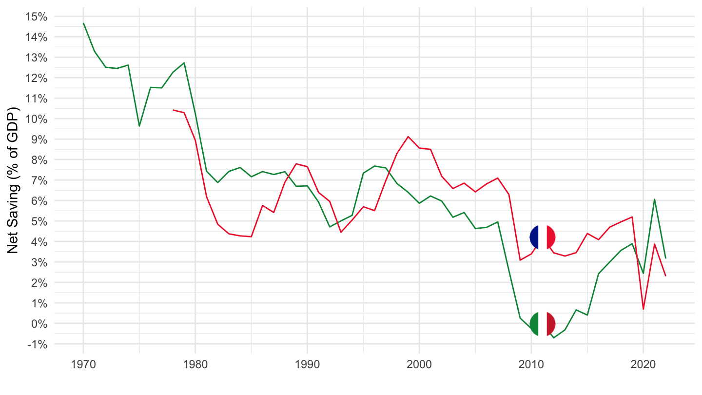

United Kingdom, Japan, United States

Code

SNA_TABLE2 %>%
  filter(MEASURE == "C",
         LOCATION %in% c("JPN", "GBR", "USA"),
         TRANSACT %in% c("B1_GE", "B8NS1")) %>%
  year_to_date %>%
  left_join(SNA_TABLE2_var$LOCATION, by = "LOCATION") %>%
  select(Location, date, TRANSACT, obsValue) %>%
  spread(TRANSACT, obsValue) %>%
  group_by(Location) %>%
  mutate(obsValue = B8NS1 / B1_GE) %>%
  select(Location, date, obsValue) %>%
  na.omit %>%
  left_join(colors, by = c("Location" = "country")) %>%
  ggplot() + geom_line(aes(x = date, y = obsValue, color = color)) +
  scale_color_identity() + theme_minimal() + add_3flags +
  scale_x_date(breaks = seq(1920, 2025, 10) %>% paste0("-01-01") %>% as.Date,
               labels = date_format("%Y")) +
  scale_y_continuous(breaks = 0.01*seq(-10, 100, 1),
                     labels = scales::percent_format(accuracy = 1)) +
  ylab("Net Saving (% of GDP)") + xlab("")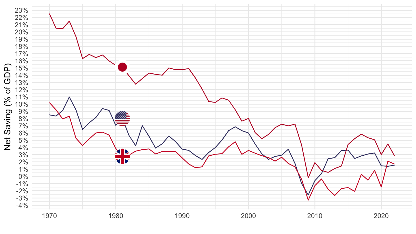

Switzerland, Germany, Netherlands

Code

SNA_TABLE2 %>%
  filter(MEASURE == "C",
         LOCATION %in% c("NLD", "CHE", "DEU"),
         TRANSACT %in% c("B1_GE", "B8NS1")) %>%
  year_to_date %>%
  left_join(SNA_TABLE2_var$LOCATION, by = "LOCATION") %>%
  select(Location, date, TRANSACT, obsValue) %>%
  spread(TRANSACT, obsValue) %>%
  group_by(Location) %>%
  mutate(obsValue = B8NS1 / B1_GE) %>%
  select(Location, date, obsValue) %>%
  left_join(colors, by = c("Location" = "country")) %>%
  ggplot() + geom_line(aes(x = date, y = obsValue, color = color)) +
  scale_color_identity() + theme_minimal() + add_3flags +
  scale_x_date(breaks = seq(1920, 2025, 10) %>% paste0("-01-01") %>% as.Date,
               labels = date_format("%Y")) +
  scale_y_continuous(breaks = 0.01*seq(-10, 100, 1),
                     labels = scales::percent_format(accuracy = 1)) +
  ylab("Net Saving (% of GDP)") + xlab("")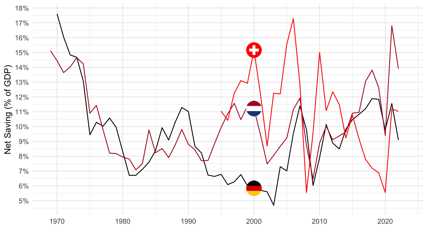

P5S1 - K1S1 - Net capital formation / GDP

France, Germany, Italy

Code

SNA_TABLE2 %>%
  filter(MEASURE == "C",
         LOCATION %in% c("FRA", "DEU", "ITA"),
         TRANSACT %in% c("B1_GE", "P5S1", "K1S1")) %>%
  year_to_date %>%
  left_join(SNA_TABLE2_var$LOCATION, by = "LOCATION") %>%
  select(Location, date, TRANSACT, obsValue) %>%
  spread(TRANSACT, obsValue) %>%
  mutate(obsValue = (P5S1 - K1S1) / B1_GE) %>%
  filter(!is.na(obsValue)) %>%
  left_join(colors, by = c("Location" = "country")) %>%
  ggplot() + geom_line(aes(x = date, y = obsValue, color = color)) +
  scale_color_identity() + theme_minimal() + add_3flags +
  scale_x_date(breaks = seq(1920, 2025, 10) %>% paste0("-01-01") %>% as.Date,
               labels = date_format("%Y")) +
  theme(legend.position = c(0.85, 0.9),
        legend.title = element_blank()) +
  scale_y_continuous(breaks = 0.01*seq(-10, 100, 1),
                     labels = scales::percent_format(accuracy = 1)) +
  ylab("Net capital formation (% of GDP)") + xlab("")

United Kingdom, Japan, United States

Code

SNA_TABLE2 %>%
  filter(MEASURE == "C",
         LOCATION %in% c("GBR", "JPN", "USA"),
         TRANSACT %in% c("B1_GE", "P5S1", "K1S1")) %>%
  year_to_date %>%
  left_join(SNA_TABLE2_var$LOCATION, by = "LOCATION") %>%
  select(Location, date, TRANSACT, obsValue) %>%
  spread(TRANSACT, obsValue) %>%
  mutate(obsValue = (P5S1 - K1S1) / B1_GE) %>%
  filter(!is.na(obsValue)) %>%
  left_join(colors, by = c("Location" = "country")) %>%
  ggplot() + geom_line(aes(x = date, y = obsValue, color = color)) +
  scale_color_identity() + theme_minimal() + add_3flags +
  scale_x_date(breaks = seq(1920, 2025, 10) %>% paste0("-01-01") %>% as.Date,
               labels = date_format("%Y")) +
  theme(legend.position = c(0.85, 0.9),
        legend.title = element_blank()) +
  scale_y_continuous(breaks = 0.01*seq(-10, 100, 1),
                     labels = scales::percent_format(accuracy = 1)) +
  ylab("Net capital formation (% of GDP)") + xlab("")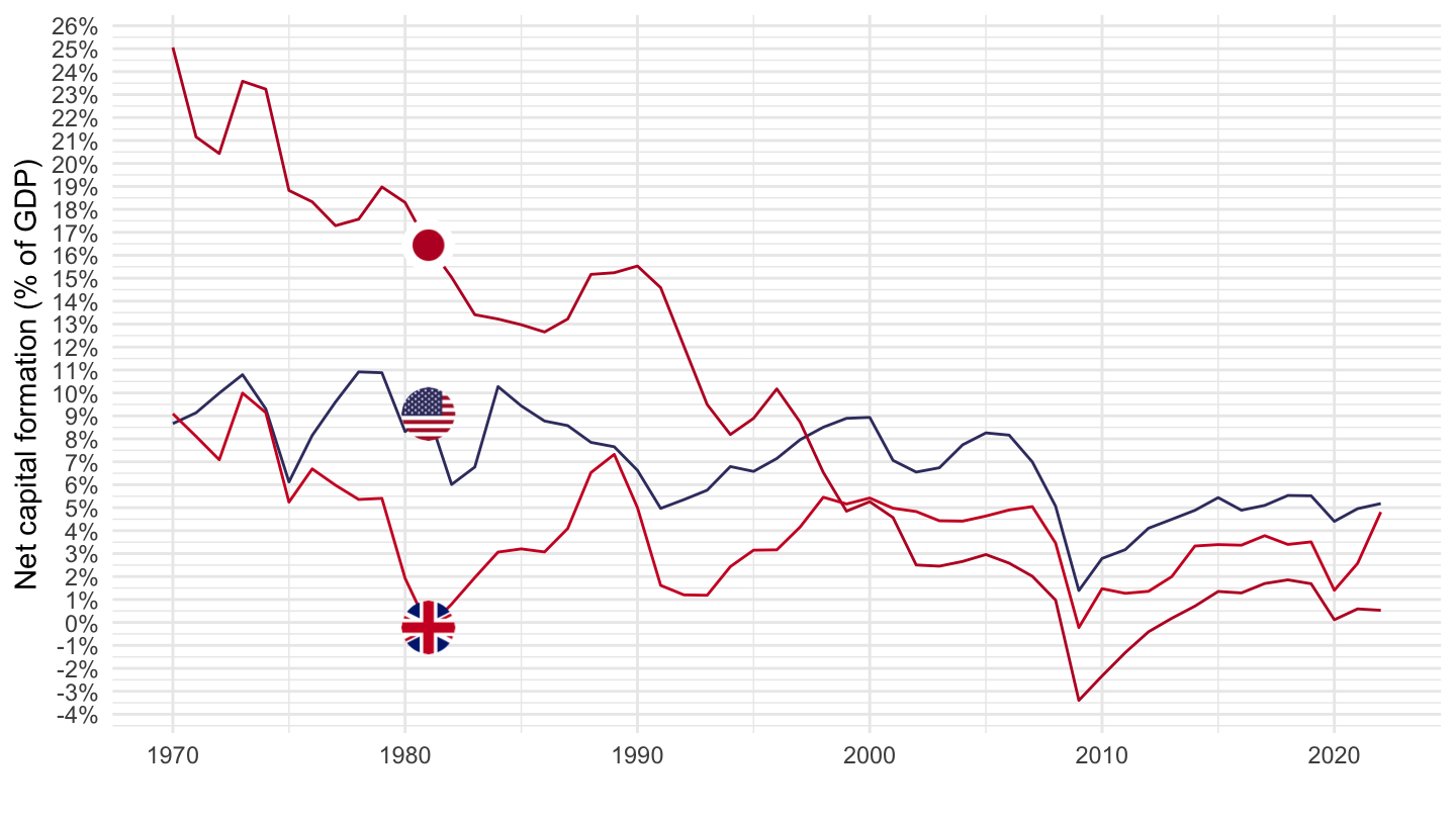

Switzerland, Germany, Netherlands

Code

SNA_TABLE2 %>%
  filter(MEASURE == "C",
         LOCATION %in% c("CHE", "DEU", "NLD"),
         TRANSACT %in% c("B1_GE", "P5S1", "K1S1")) %>%
  year_to_date %>%
  left_join(SNA_TABLE2_var$LOCATION, by = "LOCATION") %>%
  select(Location, date, TRANSACT, obsValue) %>%
  spread(TRANSACT, obsValue) %>%
  mutate(obsValue = (P5S1 - K1S1) / B1_GE) %>%
  filter(!is.na(obsValue)) %>%
  left_join(colors, by = c("Location" = "country")) %>%
  ggplot() + geom_line(aes(x = date, y = obsValue, color = color)) +
  scale_color_identity() + theme_minimal() + add_3flags +
  scale_x_date(breaks = seq(1920, 2025, 10) %>% paste0("-01-01") %>% as.Date,
               labels = date_format("%Y")) +
  theme(legend.position = c(0.85, 0.9),
        legend.title = element_blank()) +
  scale_y_continuous(breaks = 0.01*seq(-10, 100, 1),
                     labels = scales::percent_format(accuracy = 1)) +
  ylab("Net capital formation (% of GDP)") + xlab("")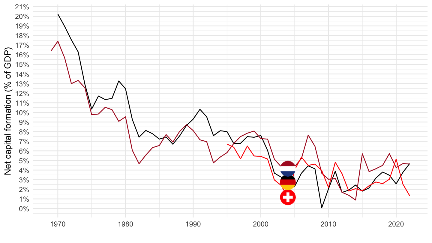

P5S1 - Gross capital formation / GDP

France, Germany, Italy

Code

SNA_TABLE2 %>%
  filter(MEASURE == "C",
         LOCATION %in% c("FRA", "DEU", "ITA"),
         TRANSACT %in% c("B1_GE", "P5S1")) %>%
  year_to_date %>%
  left_join(SNA_TABLE2_var$LOCATION, by = "LOCATION") %>%
  spread(TRANSACT, obsValue) %>%
  mutate(obsValue = (P5S1) / B1_GE) %>%
  filter(!is.na(obsValue)) %>%
  left_join(colors, by = c("Location" = "country")) %>%
  ggplot() + geom_line(aes(x = date, y = obsValue, color = color)) +
  scale_color_identity() + theme_minimal() + add_3flags +
  scale_x_date(breaks = seq(1920, 2025, 10) %>% paste0("-01-01") %>% as.Date,
               labels = date_format("%Y")) +
  theme(legend.position = c(0.85, 0.9),
        legend.title = element_blank()) +
  scale_y_continuous(breaks = 0.01*seq(-10, 100, 1),
                     labels = scales::percent_format(accuracy = 1)) +
  ylab("Gross capital formation (% of GDP)") + xlab("")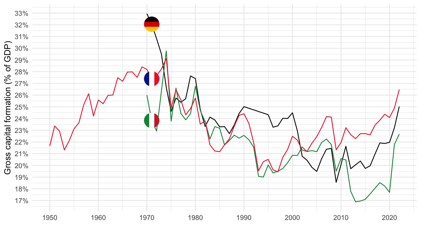

United Kingdom, Japan, United States

Code

SNA_TABLE2 %>%
  filter(MEASURE == "C",
         LOCATION %in% c("GBR", "JPN", "USA"),
         TRANSACT %in% c("B1_GE", "P5S1")) %>%
  year_to_date %>%
  left_join(SNA_TABLE2_var$LOCATION, by = "LOCATION") %>%
  spread(TRANSACT, obsValue) %>%
  mutate(obsValue = (P5S1) / B1_GE) %>%
  filter(!is.na(obsValue)) %>%
  left_join(colors, by = c("Location" = "country")) %>%
  ggplot() + geom_line(aes(x = date, y = obsValue, color = color)) +
  scale_color_identity() + theme_minimal() + add_3flags +
  scale_x_date(breaks = seq(1920, 2025, 10) %>% paste0("-01-01") %>% as.Date,
               labels = date_format("%Y")) +
  theme(legend.position = c(0.85, 0.9),
        legend.title = element_blank()) +
  scale_y_continuous(breaks = 0.01*seq(-10, 100, 1),
                     labels = scales::percent_format(accuracy = 1)) +
  ylab("Gross capital formation (% of GDP)") + xlab("")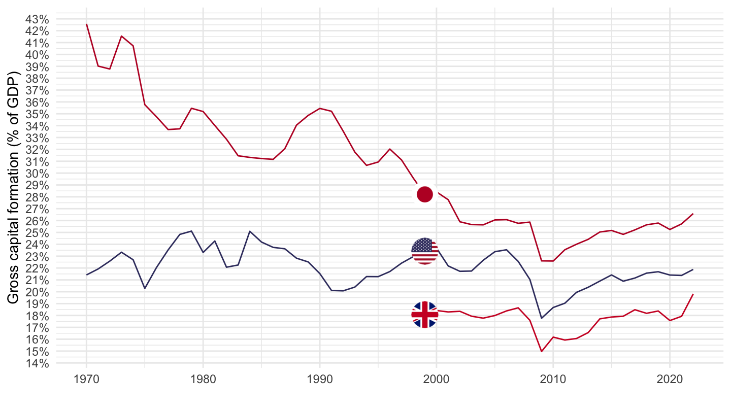

Switzerland, Germany, Netherlands

Code

SNA_TABLE2 %>%
  filter(MEASURE == "C",
         LOCATION %in% c("CHE", "DEU", "NLD"),
         TRANSACT %in% c("B1_GE", "P5S1")) %>%
  year_to_date %>%
  left_join(SNA_TABLE2_var$LOCATION, by = "LOCATION") %>%
  spread(TRANSACT, obsValue) %>%
  mutate(obsValue = (P5S1) / B1_GE) %>%
  filter(!is.na(obsValue)) %>%
  left_join(colors, by = c("Location" = "country")) %>%
  ggplot() + geom_line(aes(x = date, y = obsValue, color = color)) +
  scale_color_identity() + theme_minimal() + add_3flags +
  scale_x_date(breaks = seq(1920, 2025, 10) %>% paste0("-01-01") %>% as.Date,
               labels = date_format("%Y")) +
  theme(legend.position = c(0.85, 0.9),
        legend.title = element_blank()) +
  scale_y_continuous(breaks = 0.01*seq(-10, 100, 1),
                     labels = scales::percent_format(accuracy = 1)) +
  ylab("Gross capital formation (% of GDP)") + xlab("")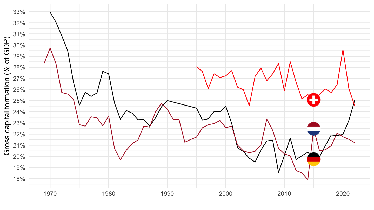

B9S1 - Net Lending - Net Borrowing / GDP

France, Germany, Italy

Code

SNA_TABLE2 %>%
  filter(MEASURE == "C",
         LOCATION %in% c("FRA", "DEU", "ITA"),
         TRANSACT %in% c("B1_GE", "B9S1")) %>%
  year_to_date %>%
  left_join(SNA_TABLE2_var$LOCATION, by = "LOCATION") %>%
  select(Location, date, TRANSACT, obsValue) %>%
  spread(TRANSACT, obsValue) %>%
  group_by(Location) %>%
  mutate(obsValue = B9S1 / B1_GE) %>%
  select(Location, date, obsValue) %>%
  na.omit %>%
  left_join(colors, by = c("Location" = "country")) %>%
  ggplot() + geom_line(aes(x = date, y = obsValue, color = color)) +
  scale_color_identity() + theme_minimal() + add_3flags +
  scale_x_date(breaks = seq(1920, 2025, 10) %>% paste0("-01-01") %>% as.Date,
               labels = date_format("%Y")) +
  scale_y_continuous(breaks = 0.01*seq(-100, 100, 5),
                     labels = scales::percent_format(accuracy = 1)) +
  ylab("Net Lending - Net Borrowing (% of GDP)") + xlab("")

France, Italy

Code

SNA_TABLE2 %>%
  filter(MEASURE == "C",
         LOCATION %in% c("FRA", "ITA"),
         TRANSACT %in% c("B1_GE", "B9S1")) %>%
  year_to_date %>%
  left_join(SNA_TABLE2_var$LOCATION, by = "LOCATION") %>%
  select(Location, date, TRANSACT, obsValue) %>%
  spread(TRANSACT, obsValue) %>%
  group_by(Location) %>%
  mutate(obsValue = B9S1 / B1_GE) %>%
  select(Location, date, obsValue) %>%
  na.omit %>%
  left_join(colors, by = c("Location" = "country")) %>%
  ggplot() + geom_line(aes(x = date, y = obsValue, color = color)) +
  scale_color_identity() + theme_minimal() + add_2flags +
  scale_x_date(breaks = seq(1920, 2025, 10) %>% paste0("-01-01") %>% as.Date,
               labels = date_format("%Y")) +
  scale_y_continuous(breaks = 0.01*seq(-100, 100, 1),
                     labels = scales::percent_format(accuracy = 1)) +
  ylab("Net Lending - Net Borrowing (% of GDP)") + xlab("")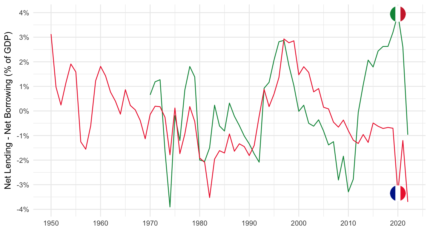

United Kingdom, Japan, United States

Code

SNA_TABLE2 %>%
  filter(MEASURE == "C",
         LOCATION %in% c("JPN", "GBR", "USA"),
         TRANSACT %in% c("B1_GE", "B9S1")) %>%
  year_to_date %>%
  left_join(SNA_TABLE2_var$LOCATION, by = "LOCATION") %>%
  select(Location, date, TRANSACT, obsValue) %>%
  spread(TRANSACT, obsValue) %>%
  group_by(Location) %>%
  mutate(obsValue = B9S1 / B1_GE) %>%
  select(Location, date, obsValue) %>%
  na.omit %>%
  left_join(colors, by = c("Location" = "country")) %>%
  ggplot() + geom_line(aes(x = date, y = obsValue, color = color)) +
  scale_color_identity() + theme_minimal() + add_3flags +
  scale_x_date(breaks = seq(1920, 2025, 10) %>% paste0("-01-01") %>% as.Date,
               labels = date_format("%Y")) +
  scale_y_continuous(breaks = 0.01*seq(-100, 100, 1),
                     labels = scales::percent_format(accuracy = 1)) +
  ylab("Net Lending - Net Borrowing (% of GDP)") + xlab("")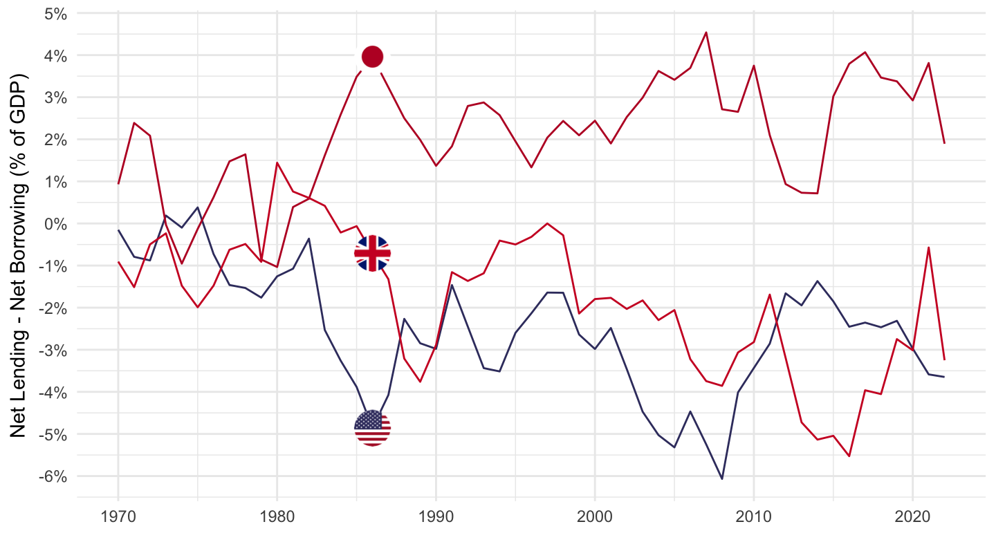

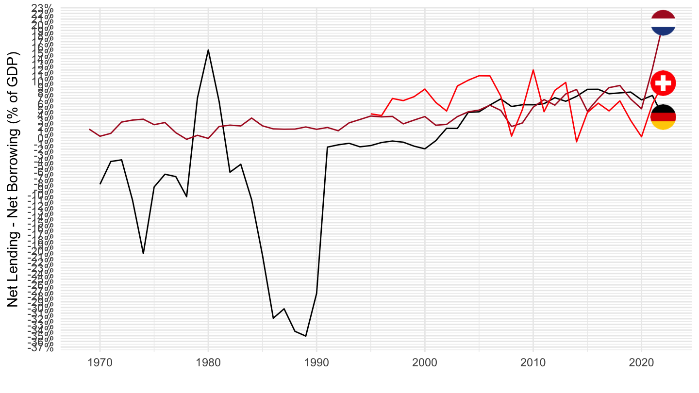
Switzerland, Germany, Netherlands

Code

SNA_TABLE2 %>%
  filter(MEASURE == "C",
         LOCATION %in% c("NLD", "CHE", "DEU"),
         TRANSACT %in% c("B1_GE", "B9S1")) %>%
  year_to_date %>%
  left_join(SNA_TABLE2_var$LOCATION, by = "LOCATION") %>%
  select(Location, date, TRANSACT, obsValue) %>%
  spread(TRANSACT, obsValue) %>%
  group_by(Location) %>%
  mutate(obsValue = B9S1 / B1_GE) %>%
  select(Location, date, obsValue) %>%
  na.omit %>%
  left_join(colors, by = c("Location" = "country")) %>%
  ggplot() + geom_line(aes(x = date, y = obsValue, color = color)) +
  scale_color_identity() + theme_minimal() + add_3flags +
  scale_x_date(breaks = seq(1920, 2025, 10) %>% paste0("-01-01") %>% as.Date,
               labels = date_format("%Y")) +
  scale_y_continuous(breaks = 0.01*seq(-100, 100, 1),
                     labels = scales::percent_format(accuracy = 1)) +
  ylab("Net Lending - Net Borrowing (% of GDP)") + xlab("")