Value added and its components by activity, ISIC rev4 - SNA_TABLE6A

Name: Value added and its components by activity, ISIC rev4
Creator: François Geerolf
License: https://creativecommons.org/licenses/by/4.0/

Data - OECD

Author

François Geerolf

Last observation: 2023 (N = 3)

First observation: 1960 (N = 302)

Last data update: 02 août 2026, 09:11

Last compile: 06 sept. 2026, 15:02

Structure

obsTime

Code

SNA_TABLE6A |>
  group_by(obsTime) |>
  summarise(Nobs = n()) |>
  arrange(desc(obsTime)) |>
  print_table_conditional()

Real Estate

Table

Code

SNA_TABLE6A |>
  filter(TRANSACT %in% c("B1GA", "B1_GE"),
         ACTIVITY %in% c("VL", "VTOT"),
         MEASURE == "C") |>
  left_join(SNA_TABLE6A_var$LOCATION, by = "LOCATION") |>
  year_to_date() |>
  mutate(VARIABLE = paste0(TRANSACT, "_", ACTIVITY)) |>
  select(VARIABLE, LOCATION, Location, date, obsValue) |>
  spread(VARIABLE, obsValue) |>
  mutate(value = B1GA_VL / B1_GE_VTOT) |>
  filter(!is.na(value)) |>
  group_by(LOCATION, Location) |>
  summarise(year1 = first(year(date)),
            value1 = first(value),
            year2 = last(year(date)),
            value2 = last(value)) %>%
  mutate_at(vars(value1, value2), funs(round(100*., digits = 1))) |>
  arrange(value2) |>
  mutate(Flag = gsub(" ", "-", str_to_lower(gsub(" ", "-", Location))),
         Flag = paste0('<img src="../../icon/flag/vsmall/', Flag, '.png" alt="Flag">')) |>
  select(Flag, everything()) %>%
  {if (is_html_output()) datatable(., filter = 'top', rownames = F, escape = F) else .}

France, Greece, Italy, Spain

All

Code

SNA_TABLE6A |>
  filter(TRANSACT %in% c("B1GA", "B1_GE"),
         ACTIVITY %in% c("VL", "VTOT"),
         LOCATION %in% c("GRC", "FRA", "ITA", "ESP"),
         MEASURE == "C") |>
  left_join(SNA_TABLE6A_var$LOCATION, by = "LOCATION") |>
  year_to_date() |>
  mutate(VARIABLE = paste0(TRANSACT, "_", ACTIVITY)) |>
  select(VARIABLE, Location, date, obsValue) |>
  spread(VARIABLE, obsValue) |>
  mutate(obsValue = B1GA_VL / B1_GE_VTOT) |>
  na.omit() |>
  add_flag_color("Location") |>
  ggplot() + geom_line(aes(x = date, y = obsValue, color = color)) + 
  scale_color_identity() + add_4flags + theme_minimal() +
  scale_x_date(breaks = seq(1920, 2100, 5) |> paste0("-01-01") |> as.Date(),
               labels = date_format("%Y")) +
  scale_y_continuous(breaks = 0.01*seq(-7, 26, 1),
                     labels = scales::percent_format(accuracy = 1)) +
  ylab("Value Added in Real Estate (% of GDP)") + xlab("")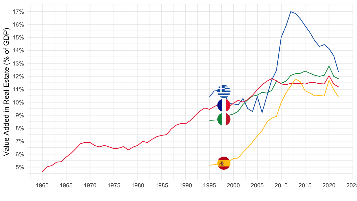

1995-

Code

SNA_TABLE6A |>
  filter(TRANSACT %in% c("B1GA", "B1_GE"),
         ACTIVITY %in% c("VL", "VTOT"),
         LOCATION %in% c("GRC", "FRA", "ITA", "ESP"),
         MEASURE == "C") |>
  left_join(SNA_TABLE6A_var$LOCATION, by = "LOCATION") |>
  year_to_date() |>
  filter(date >= as.Date("1995-01-01")) |>
  mutate(VARIABLE = paste0(TRANSACT, "_", ACTIVITY)) |>
  select(VARIABLE, Location, date, obsValue) |>
  spread(VARIABLE, obsValue) |>
  mutate(obsValue = B1GA_VL / B1_GE_VTOT) |>
  na.omit() |>
  add_flag_color("Location") |>
  ggplot() + geom_line(aes(x = date, y = obsValue, color = color)) + 
  scale_color_identity() + add_4flags + theme_minimal() +
  scale_x_date(breaks = seq(1920, 2100, 5) |> paste0("-01-01") |> as.Date(),
               labels = date_format("%Y")) +
  scale_y_continuous(breaks = 0.01*seq(-7, 26, 1),
                     labels = scales::percent_format(accuracy = 1)) +
  ylab("Value Added in Real Estate (% of GDP)") + xlab("")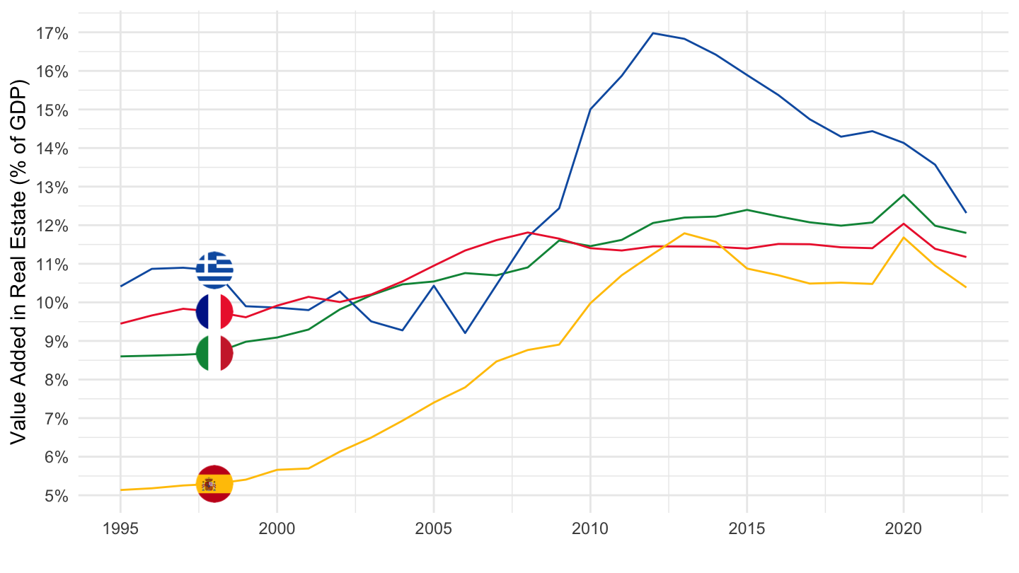

France, Germany, US

Code

SNA_TABLE6A |>
  filter(TRANSACT %in% c("B1GA", "B1_GE"),
         ACTIVITY %in% c("VL", "VTOT"),
         LOCATION %in% c("FRA", "DEU", "USA"),
         MEASURE == "C") |>
  left_join(SNA_TABLE6A_var$LOCATION, by = "LOCATION") |>
  year_to_date() |>
  mutate(VARIABLE = paste0(TRANSACT, "_", ACTIVITY)) |>
  select(VARIABLE, Location, date, obsValue) |>
  spread(VARIABLE, obsValue) |>
  mutate(obsValue = B1GA_VL / B1_GE_VTOT) |>
  na.omit() |>
  add_flag_color("Location") |>
  ggplot() + geom_line(aes(x = date, y = obsValue, color = color)) + 
  scale_color_identity() + add_3flags + theme_minimal() +
  scale_x_date(breaks = seq(1920, 2100, 5) |> paste0("-01-01") |> as.Date(),
               labels = date_format("%Y")) +
  scale_y_continuous(breaks = 0.01*seq(-7, 26, 1),
                     labels = scales::percent_format(accuracy = 1)) +
  ylab("Value Added in Real Estate (% of GDP)") + xlab("")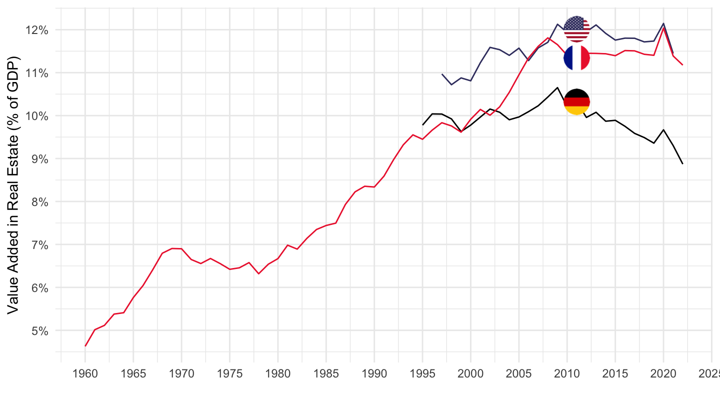

New Zealand, UK, US

Code

SNA_TABLE6A |>
  filter(TRANSACT %in% c("B1GA", "B1_GE"),
         ACTIVITY %in% c("VL", "VTOT"),
         LOCATION %in% c("GBR", "NZL", "USA"),
         MEASURE == "C") |>
  left_join(SNA_TABLE6A_var$LOCATION, by = "LOCATION") |>
  year_to_date() |>
  mutate(VARIABLE = paste0(TRANSACT, "_", ACTIVITY)) |>
  select(VARIABLE, Location, date, obsValue) |>
  spread(VARIABLE, obsValue) |>
  mutate(obsValue = B1GA_VL / B1_GE_VTOT) |>
  na.omit() |>
  add_flag_color("Location") |>
  ggplot() + geom_line(aes(x = date, y = obsValue, color = color)) + 
  scale_color_identity() + add_3flags + theme_minimal() +
  scale_x_date(breaks = seq(1920, 2100, 5) |> paste0("-01-01") |> as.Date(),
               labels = date_format("%Y")) +
  scale_y_continuous(breaks = 0.01*seq(-7, 26, 1),
                     labels = scales::percent_format(accuracy = 1)) +
  ylab("Value Added in Real Estate (% of GDP)") + xlab("")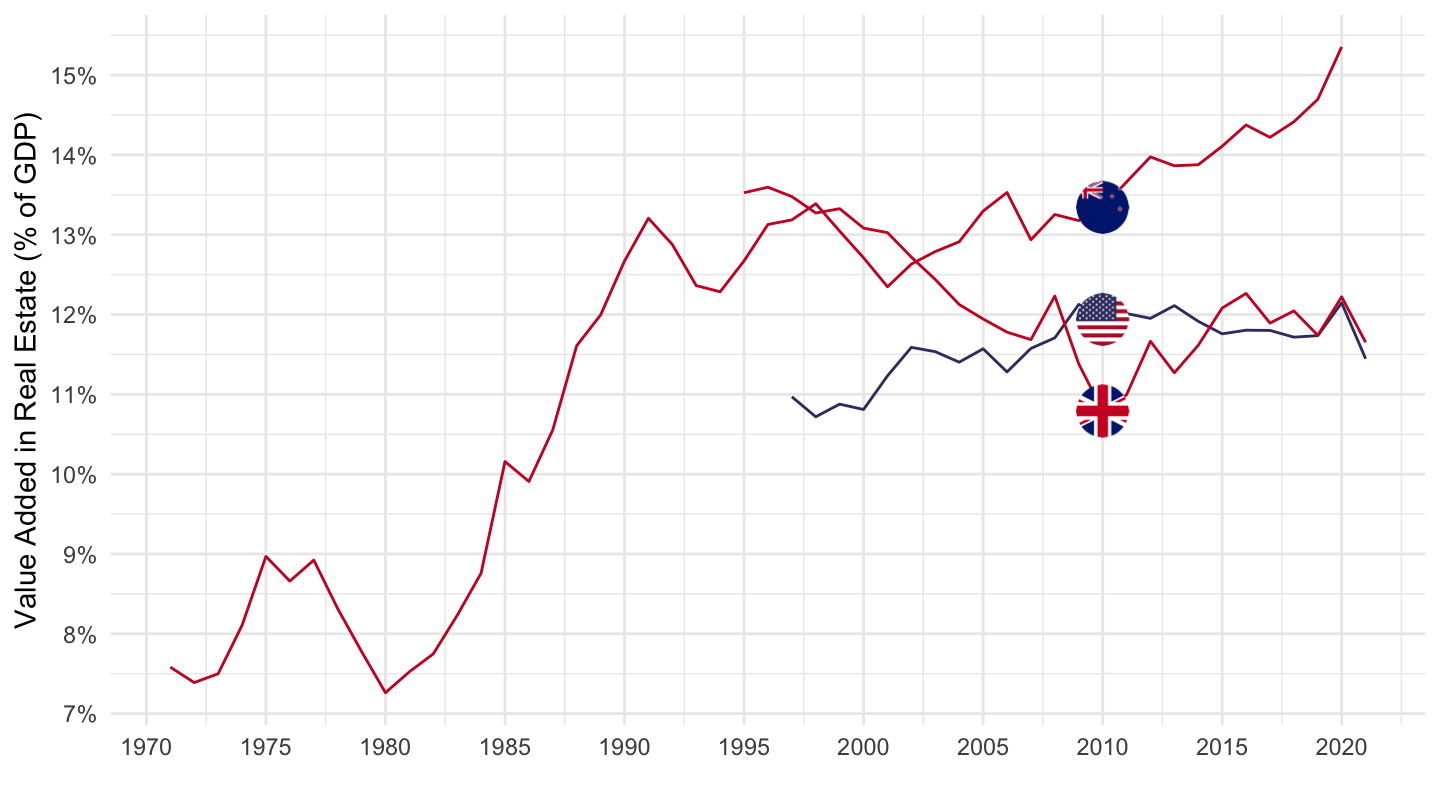

Low Manufacturing

Table

Code

SNA_TABLE6A |>
  filter(TRANSACT %in% c("B1GA", "B1_GE"),
         ACTIVITY %in% c("VC", "VTOT"),
         MEASURE == "C") |>
  left_join(SNA_TABLE6A_var$LOCATION, by = "LOCATION") |>
  year_to_date() |>
  mutate(VARIABLE = paste0(TRANSACT, "_", ACTIVITY)) |>
  select(VARIABLE, LOCATION, Location, date, obsValue) |>
  spread(VARIABLE, obsValue) |>
  mutate(value = B1GA_VC / B1_GE_VTOT) |>
  filter(!is.na(value)) |>
  group_by(LOCATION, Location) |>
  summarise(year1 = first(year(date)),
            value1 = first(value),
            year2 = last(year(date)),
            value2 = last(value)) %>%
  mutate_at(vars(value1, value2), funs(round(100*., digits = 1))) |>
  arrange(value2) |>
  mutate(Flag = gsub(" ", "-", str_to_lower(gsub(" ", "-", Location))),
         Flag = paste0('<img src="../../icon/flag/vsmall/', Flag, '.png" alt="Flag">')) |>
  select(Flag, everything()) %>%
  {if (is_html_output()) datatable(., filter = 'top', rownames = F, escape = F) else .}

Luxembourg, Cyprus, Australia

Code

SNA_TABLE6A |>
  filter(TRANSACT %in% c("B1GA", "B1_GE"),
         ACTIVITY %in% c("VC", "VTOT"),
         LOCATION %in% c("LUX", "CYP", "AUS"),
         MEASURE == "C") |>
  left_join(SNA_TABLE6A_var$LOCATION, by = "LOCATION") |>
  year_to_date() |>
  mutate(VARIABLE = paste0(TRANSACT, "_", ACTIVITY)) |>
  select(VARIABLE, Location, date, obsValue) |>
  spread(VARIABLE, obsValue) |>
  mutate(obsValue = B1GA_VC / B1_GE_VTOT) |>
  na.omit() |>
  add_flag_color("Location") |>
  ggplot() + geom_line(aes(x = date, y = obsValue, color = color)) + 
  scale_color_identity() + add_3flags + theme_minimal() +
  scale_x_date(breaks = seq(1920, 2100, 5) |> paste0("-01-01") |> as.Date(),
               labels = date_format("%Y")) +
  scale_y_continuous(breaks = 0.01*seq(-7, 26, 1),
                     labels = scales::percent_format(accuracy = 1)) +
  ylab("Value Added in Manufacturing (% of GDP)") + xlab("")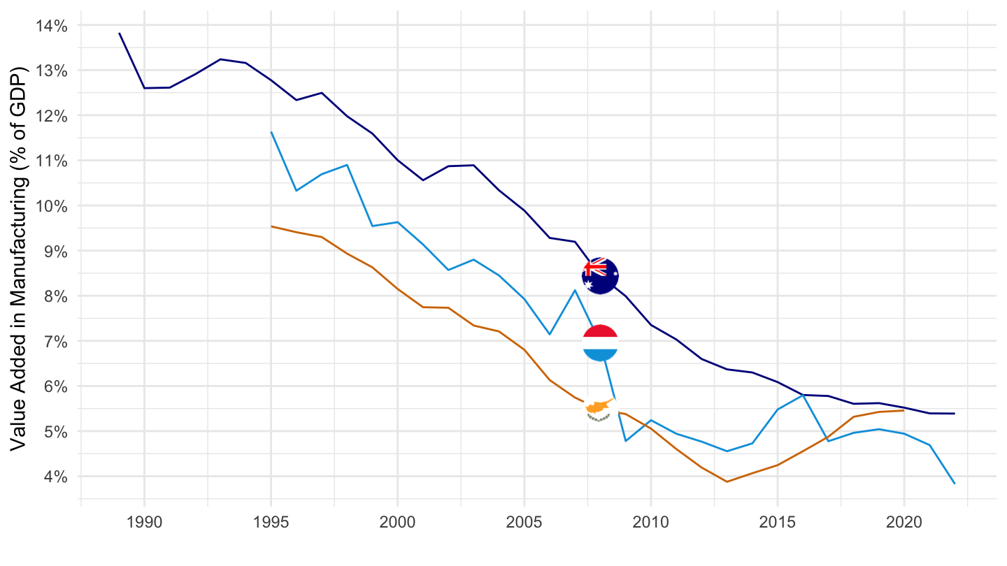

Albania, Norway, Greece

Code

SNA_TABLE6A |>
  filter(TRANSACT %in% c("B1GA", "B1_GE"),
         ACTIVITY %in% c("VC", "VTOT"),
         LOCATION %in% c("ALB", "NOR", "GRC"),
         MEASURE == "C") |>
  left_join(SNA_TABLE6A_var$LOCATION, by = "LOCATION") |>
  year_to_date() |>
  mutate(VARIABLE = paste0(TRANSACT, "_", ACTIVITY)) |>
  select(VARIABLE, Location, date, obsValue) |>
  spread(VARIABLE, obsValue) |>
  mutate(obsValue = B1GA_VC / B1_GE_VTOT) |>
  na.omit() |>
  add_flag_color("Location") |>
  ggplot() + geom_line(aes(x = date, y = obsValue, color = color)) + 
  scale_color_identity() + add_3flags + theme_minimal() +
  scale_x_date(breaks = seq(1920, 2100, 5) |> paste0("-01-01") |> as.Date(),
               labels = date_format("%Y")) +
  scale_y_continuous(breaks = 0.01*seq(-7, 26, 1),
                     labels = scales::percent_format(accuracy = 1)) +
  ylab("Value Added in Manufacturing (% of GDP)") + xlab("")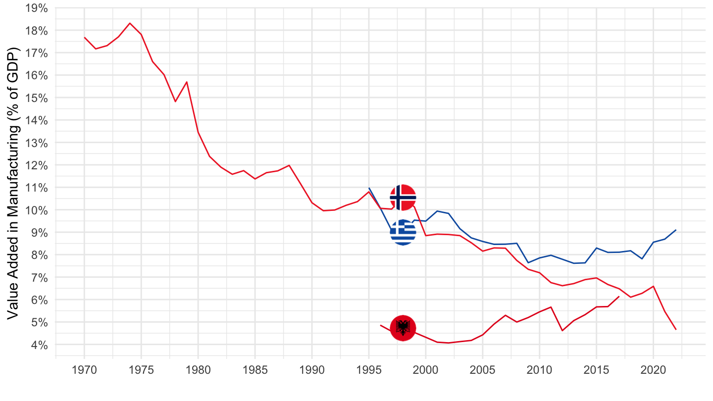

Malta, Iceland, United Kingdom

Code

SNA_TABLE6A |>
  filter(TRANSACT %in% c("B1GA", "B1_GE"),
         ACTIVITY %in% c("VC", "VTOT"),
         LOCATION %in% c("MLT", "ISL", "GBR"),
         MEASURE == "C") |>
  left_join(SNA_TABLE6A_var$LOCATION, by = "LOCATION") |>
  year_to_date() |>
  mutate(VARIABLE = paste0(TRANSACT, "_", ACTIVITY)) |>
  select(LOCATION, VARIABLE, Location, date, obsValue) |>
  spread(VARIABLE, obsValue) |>
  mutate(obsValue = B1GA_VC / B1_GE_VTOT) |>
  na.omit() |>
  add_flag_color("Location") |>
  ggplot() + geom_line(aes(x = date, y = obsValue, color = color)) + 
  scale_color_identity() + add_3flags + theme_minimal() +
  scale_x_date(breaks = seq(1920, 2100, 5) |> paste0("-01-01") |> as.Date(),
               labels = date_format("%Y")) +
  scale_y_continuous(breaks = 0.01*seq(-7, 26, 1),
                     labels = scales::percent_format(accuracy = 1)) +
  ylab("Value Added in Manufacturing (% of GDP)") + xlab("")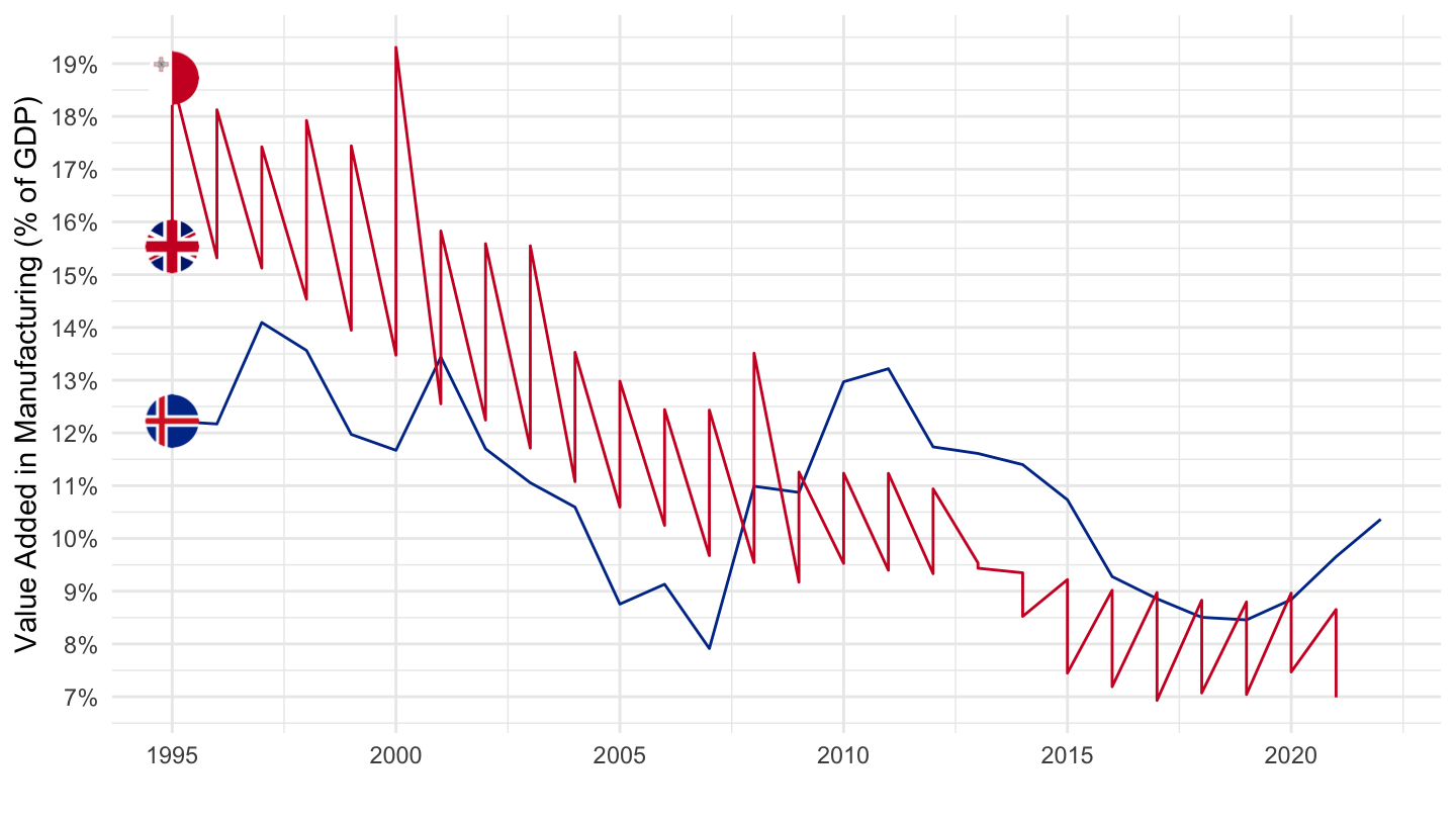

Chile, Canada, France

All

Code

SNA_TABLE6A |>
  filter(TRANSACT %in% c("B1GA", "B1_GE"),
         ACTIVITY %in% c("VC", "VTOT"),
         LOCATION %in% c("CHL", "CAN", "FRA"),
         MEASURE == "C") |>
  left_join(SNA_TABLE6A_var$LOCATION, by = "LOCATION") |>
  year_to_date() |>
  mutate(VARIABLE = paste0(TRANSACT, "_", ACTIVITY)) |>
  select(LOCATION, VARIABLE, Location, date, obsValue) |>
  spread(VARIABLE, obsValue) |>
  mutate(obsValue = B1GA_VC / B1_GE_VTOT) |>
  na.omit() |>
  add_flag_color("Location") |>
  ggplot() + geom_line(aes(x = date, y = obsValue, color = color)) + 
  scale_color_identity() + add_3flags + theme_minimal() +
  scale_x_date(breaks = seq(1920, 2100, 5) |> paste0("-01-01") |> as.Date(),
               labels = date_format("%Y")) +
  scale_y_continuous(breaks = 0.01*seq(-7, 26, 1),
                     labels = scales::percent_format(accuracy = 1)) +
  ylab("Value Added in Manufacturing (% of GDP)") + xlab("")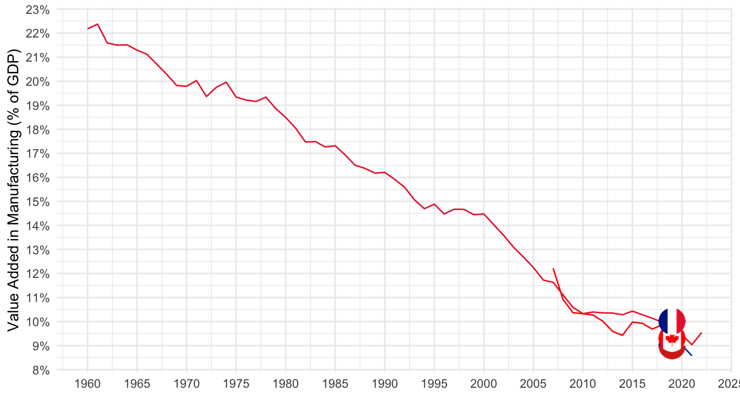

2007-

Code

SNA_TABLE6A |>
  filter(TRANSACT %in% c("B1GA", "B1_GE"),
         ACTIVITY %in% c("VC", "VTOT"),
         LOCATION %in% c("CHL", "CAN", "FRA"),
         MEASURE == "C") |>
  left_join(SNA_TABLE6A_var$LOCATION, by = "LOCATION") |>
  year_to_date() |>
  filter(date >= as.Date("2007-01-01")) |>
  mutate(VARIABLE = paste0(TRANSACT, "_", ACTIVITY)) |>
  select(LOCATION, VARIABLE, Location, date, obsValue) |>
  spread(VARIABLE, obsValue) |>
  mutate(obsValue = B1GA_VC / B1_GE_VTOT) |>
  na.omit() |>
  add_flag_color("Location") |>
  ggplot() + geom_line(aes(x = date, y = obsValue, color = color)) + 
  scale_color_identity() + add_3flags + theme_minimal() +
  scale_x_date(breaks = seq(1920, 2100, 1) |> paste0("-01-01") |> as.Date(),
               labels = date_format("%Y")) +
  scale_y_continuous(breaks = 0.01*seq(-7, 26, 1),
                     labels = scales::percent_format(accuracy = 1)) +
  ylab("Value Added in Manufacturing (% of GDP)") + xlab("")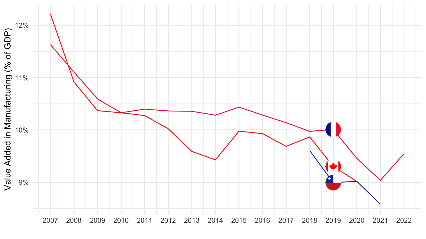

New Zealand, Latvia, Brazil

Code

SNA_TABLE6A |>
  filter(TRANSACT %in% c("B1GA", "B1_GE"),
         ACTIVITY %in% c("VC", "VTOT"),
         LOCATION %in% c("NZL", "LVA", "BRA"),
         MEASURE == "C") |>
  left_join(SNA_TABLE6A_var$LOCATION, by = "LOCATION") |>
  year_to_date() |>
  mutate(VARIABLE = paste0(TRANSACT, "_", ACTIVITY)) |>
  select(LOCATION, VARIABLE, Location, date, obsValue) |>
  spread(VARIABLE, obsValue) |>
  mutate(obsValue = B1GA_VC / B1_GE_VTOT) |>
  na.omit() |>
  add_flag_color("Location") |>
  ggplot() + geom_line(aes(x = date, y = obsValue, color = color)) + 
  scale_color_identity() + add_3flags + theme_minimal() +
  scale_x_date(breaks = seq(1920, 2100, 5) |> paste0("-01-01") |> as.Date(),
               labels = date_format("%Y")) +
  scale_y_continuous(breaks = 0.01*seq(-7, 26, 1),
                     labels = scales::percent_format(accuracy = 1)) +
  ylab("Value Added in Manufacturing (% of GDP)") + xlab("")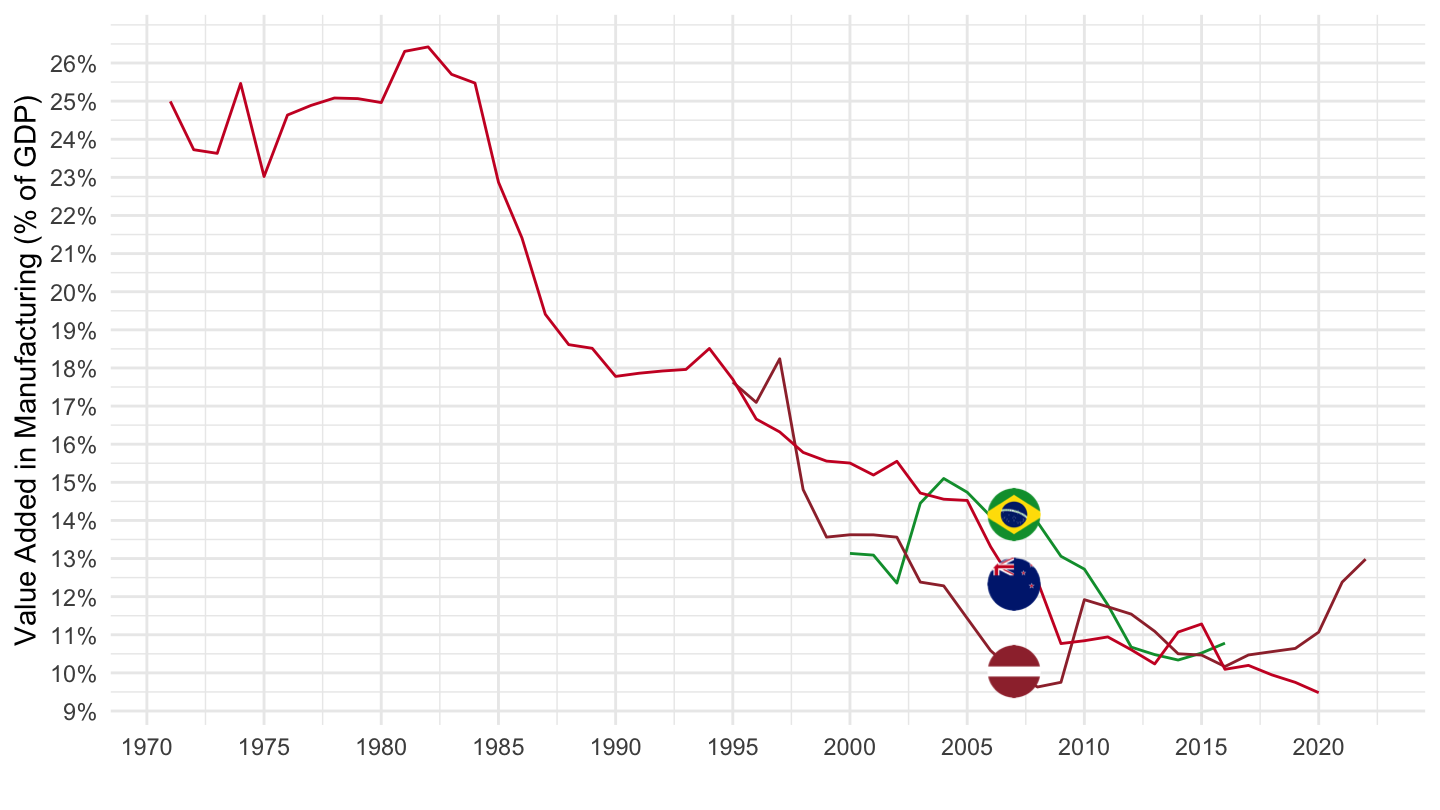

Netherlands, United States, Costa Rica

Code

SNA_TABLE6A |>
  filter(TRANSACT %in% c("B1GA", "B1_GE"),
         ACTIVITY %in% c("VC", "VTOT"),
         LOCATION %in% c("NLD", "USA", "CRI"),
         MEASURE == "C") |>
  left_join(SNA_TABLE6A_var$LOCATION, by = "LOCATION") |>
  year_to_date() |>
  mutate(VARIABLE = paste0(TRANSACT, "_", ACTIVITY)) |>
  select(LOCATION, VARIABLE, Location, date, obsValue) |>
  spread(VARIABLE, obsValue) |>
  mutate(obsValue = B1GA_VC / B1_GE_VTOT) |>
  na.omit() |>
  add_flag_color("Location") |>
  ggplot() + geom_line(aes(x = date, y = obsValue, color = color)) + 
  scale_color_identity() + add_3flags + theme_minimal() +
  scale_x_date(breaks = seq(1920, 2100, 5) |> paste0("-01-01") |> as.Date(),
               labels = date_format("%Y")) +
  scale_y_continuous(breaks = 0.01*seq(-7, 26, 1),
                     labels = scales::percent_format(accuracy = 1)) +
  ylab("Value Added in Manufacturing (% of GDP)") + xlab("")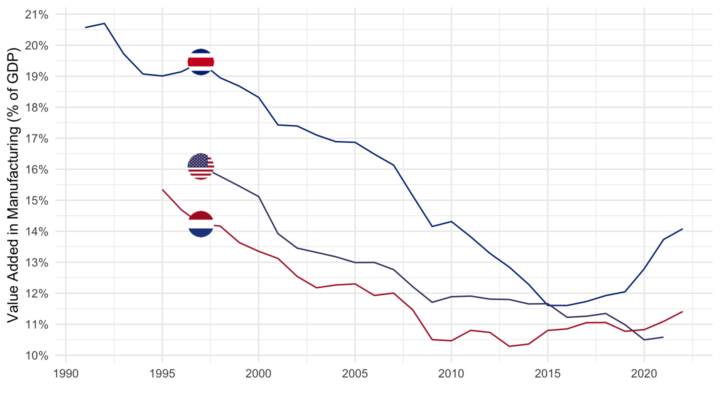

Spain, Colombia, Portugal

Code

SNA_TABLE6A |>
  filter(TRANSACT %in% c("B1GA", "B1_GE"),
         ACTIVITY %in% c("VC", "VTOT"),
         LOCATION %in% c("ESP", "COL", "PRT"),
         MEASURE == "C") |>
  left_join(SNA_TABLE6A_var$LOCATION, by = "LOCATION") |>
  year_to_date() |>
  mutate(VARIABLE = paste0(TRANSACT, "_", ACTIVITY)) |>
  select(LOCATION, VARIABLE, Location, date, obsValue) |>
  spread(VARIABLE, obsValue) |>
  mutate(obsValue = B1GA_VC / B1_GE_VTOT) |>
  na.omit() |>
  add_flag_color("Location") |>
  ggplot() + geom_line(aes(x = date, y = obsValue, color = color)) + 
  scale_color_identity() + add_3flags + theme_minimal() +
  scale_x_date(breaks = seq(1920, 2100, 5) |> paste0("-01-01") |> as.Date(),
               labels = date_format("%Y")) +
  scale_y_continuous(breaks = 0.01*seq(-7, 26, 1),
                     labels = scales::percent_format(accuracy = 1)) +
  ylab("Value Added in Manufacturing (% of GDP)") + xlab("")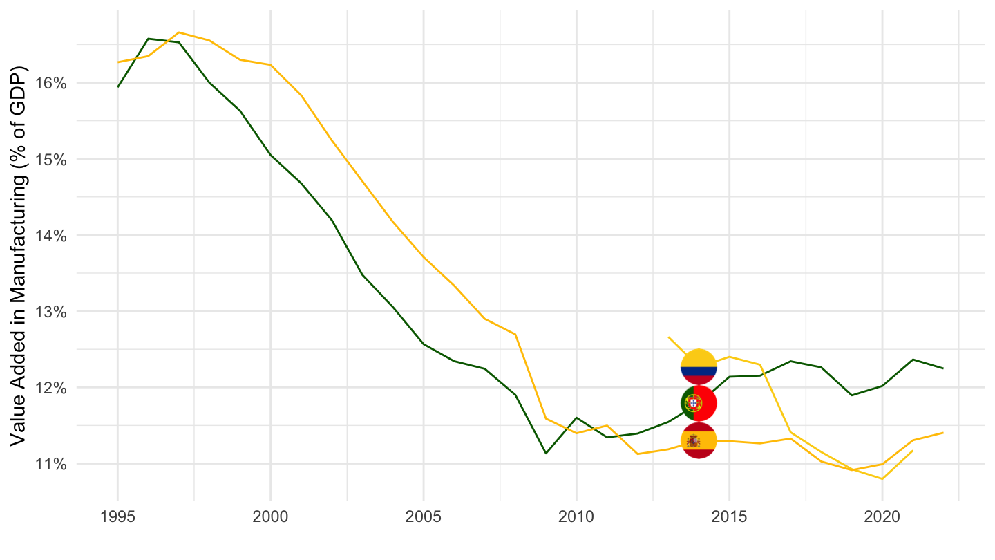

High Manufacturing

Table

Code

SNA_TABLE6A |>
  filter(TRANSACT %in% c("B1GA", "B1_GE"),
         ACTIVITY %in% c("VC", "VTOT"),
         MEASURE == "C") |>
  left_join(SNA_TABLE6A_var$LOCATION, by = "LOCATION") |>
  year_to_date() |>
  mutate(VARIABLE = paste0(TRANSACT, "_", ACTIVITY)) |>
  select(VARIABLE, LOCATION, Location, date, obsValue) |>
  spread(VARIABLE, obsValue) |>
  mutate(value = B1GA_VC / B1_GE_VTOT) |>
  filter(!is.na(value)) |>
  group_by(LOCATION, Location) |>
  summarise(year1 = first(year(date)),
            value1 = first(value),
            year2 = last(year(date)),
            value2 = last(value)) %>%
  mutate_at(vars(value1, value2), funs(round(100*., digits = 1))) |>
  arrange(-value2) |>
  mutate(Flag = gsub(" ", "-", str_to_lower(gsub(" ", "-", Location))),
         Flag = paste0('<img src="../../icon/flag/vsmall/', Flag, '.png" alt="Flag">')) |>
  select(Flag, everything()) %>%
  {if (is_html_output()) datatable(., filter = 'top', rownames = F, escape = F) else .}

Ireland, South Korea, Czech Republic

Code

SNA_TABLE6A |>
  filter(TRANSACT %in% c("B1GA", "B1_GE"),
         ACTIVITY %in% c("VC", "VTOT"),
         LOCATION %in% c("IRL", "KOR", "CZE"),
         MEASURE == "C") |>
  left_join(SNA_TABLE6A_var$LOCATION, by = "LOCATION") |>
  year_to_date() |>
  mutate(VARIABLE = paste0(TRANSACT, "_", ACTIVITY)) |>
  select(VARIABLE, Location, date, obsValue) |>
  spread(VARIABLE, obsValue) |>
  mutate(obsValue = B1GA_VC / B1_GE_VTOT) |>
  na.omit() |>
  add_flag_color("Location") |>
  ggplot() + geom_line(aes(x = date, y = obsValue, color = color)) + 
  scale_color_identity() + add_3flags + theme_minimal() +
  scale_x_date(breaks = seq(1920, 2100, 5) |> paste0("-01-01") |> as.Date(),
               labels = date_format("%Y")) +
  scale_y_continuous(breaks = 0.01*seq(0, 40, 2),
                     labels = scales::percent_format(accuracy = 1)) +
  ylab("Value Added in Manufacturing (% of GDP)") + xlab("")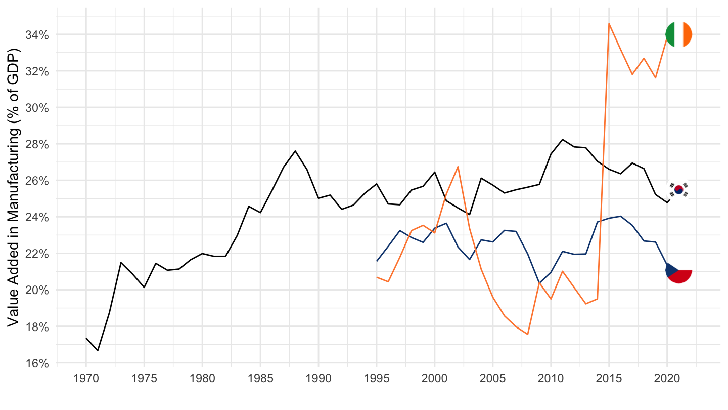

Slovenia, Germany, Romania

Code

SNA_TABLE6A |>
  filter(TRANSACT %in% c("B1GA", "B1_GE"),
         ACTIVITY %in% c("VC", "VTOT"),
         LOCATION %in% c("SVN", "DEU", "ROU"),
         MEASURE == "C") |>
  left_join(SNA_TABLE6A_var$LOCATION, by = "LOCATION") |>
  year_to_date() |>
  mutate(VARIABLE = paste0(TRANSACT, "_", ACTIVITY)) |>
  select(VARIABLE, Location, date, obsValue) |>
  spread(VARIABLE, obsValue) |>
  mutate(obsValue = B1GA_VC / B1_GE_VTOT) |>
  na.omit() |>
  add_flag_color("Location") |>
  ggplot() + geom_line(aes(x = date, y = obsValue, color = color)) + 
  scale_color_identity() + add_3flags + theme_minimal() +
  scale_x_date(breaks = seq(1920, 2100, 5) |> paste0("-01-01") |> as.Date(),
               labels = date_format("%Y")) +
  scale_y_continuous(breaks = 0.01*seq(0, 40, 1),
                     labels = scales::percent_format(accuracy = 1)) +
  ylab("Value Added in Manufacturing (% of GDP)") + xlab("")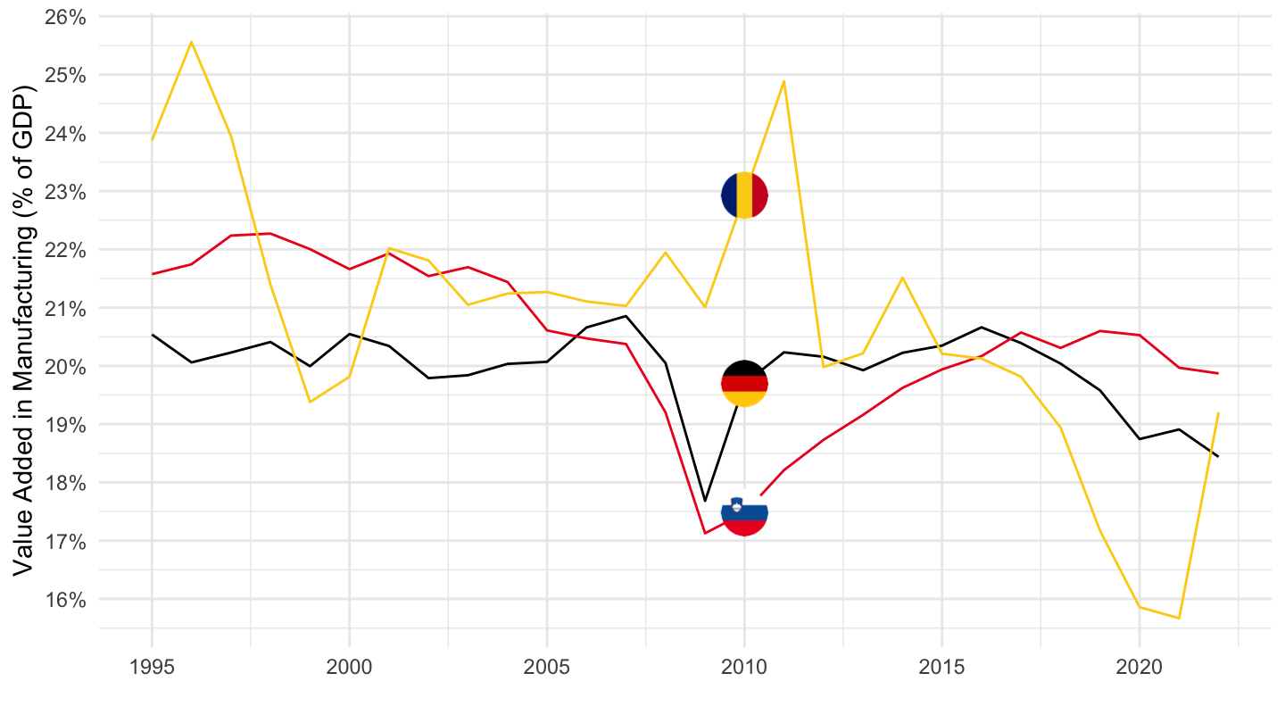

Turkey, Switzerland, Slovak Republic

Code

SNA_TABLE6A |>
  filter(TRANSACT %in% c("B1GA", "B1_GE"),
         ACTIVITY %in% c("VC", "VTOT"),
         LOCATION %in% c("TUR", "CHE", "SVK"),
         MEASURE == "C") |>
  left_join(SNA_TABLE6A_var$LOCATION, by = "LOCATION") |>
  year_to_date() |>
  mutate(VARIABLE = paste0(TRANSACT, "_", ACTIVITY)) |>
  select(LOCATION, VARIABLE, Location, date, obsValue) |>
  spread(VARIABLE, obsValue) |>
  mutate(obsValue = B1GA_VC / B1_GE_VTOT) |>
  na.omit() |>
  add_flag_color("Location") |>
  ggplot() + geom_line(aes(x = date, y = obsValue, color = color)) + 
  scale_color_identity() + add_3flags + theme_minimal() +
  scale_x_date(breaks = seq(1920, 2100, 5) |> paste0("-01-01") |> as.Date(),
               labels = date_format("%Y")) +
  scale_y_continuous(breaks = 0.01*seq(0, 40, 1),
                     labels = scales::percent_format(accuracy = 1)) +
  ylab("Value Added in Manufacturing (% of GDP)") + xlab("")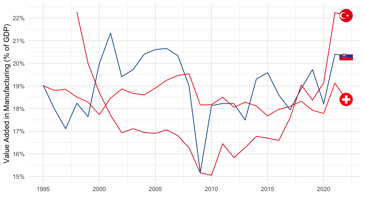

Manufacturing

Table

Code

SNA_TABLE6A |>
  filter(TRANSACT %in% c("B1GA", "B1_GE"),
         ACTIVITY %in% c("VC", "VTOT"),
         MEASURE == "C") |>
  left_join(SNA_TABLE6A_var$LOCATION, by = "LOCATION") |>
  year_to_date() |>
  mutate(VARIABLE = paste0(TRANSACT, "_", ACTIVITY)) |>
  select(VARIABLE, LOCATION, Location, date, obsValue) |>
  spread(VARIABLE, obsValue) |>
  mutate(value = B1GA_VC / B1_GE_VTOT) |>
  filter(!is.na(value)) |>
  group_by(LOCATION, Location) |>
  summarise(year1 = first(year(date)),
            value1 = first(value),
            year2 = last(year(date)),
            value2 = last(value)) %>%
  mutate_at(vars(value1, value2), funs(round(100*., digits = 1))) |>
  arrange(value2) |>
  mutate(Flag = gsub(" ", "-", str_to_lower(gsub(" ", "-", Location))),
         Flag = paste0('<img src="../../icon/flag/vsmall/', Flag, '.png" alt="Flag">')) |>
  select(Flag, everything()) %>%
  {if (is_html_output()) datatable(., filter = 'top', rownames = F, escape = F) else .}

France, Germany, US

Code

SNA_TABLE6A |>
  filter(TRANSACT %in% c("B1GA", "B1_GE"),
         ACTIVITY %in% c("VC", "VTOT"),
         LOCATION %in% c("FRA", "DEU", "USA"),
         MEASURE == "C") |>
  left_join(SNA_TABLE6A_var$LOCATION, by = "LOCATION") |>
  year_to_date() |>
  mutate(VARIABLE = paste0(TRANSACT, "_", ACTIVITY)) |>
  select(VARIABLE, Location, date, obsValue) |>
  spread(VARIABLE, obsValue) |>
  mutate(obsValue = B1GA_VC / B1_GE_VTOT) |>
  na.omit() |>
  add_flag_color("Location") |>
  ggplot() + geom_line(aes(x = date, y = obsValue, color = color)) + 
  scale_color_identity() + add_3flags + theme_minimal() +
  scale_x_date(breaks = seq(1920, 2100, 5) |> paste0("-01-01") |> as.Date(),
               labels = date_format("%Y")) +
  scale_y_continuous(breaks = 0.01*seq(-7, 26, 1),
                     labels = scales::percent_format(accuracy = 1)) +
  ylab("Value Added in Manufacturing (% of GDP)") + xlab("")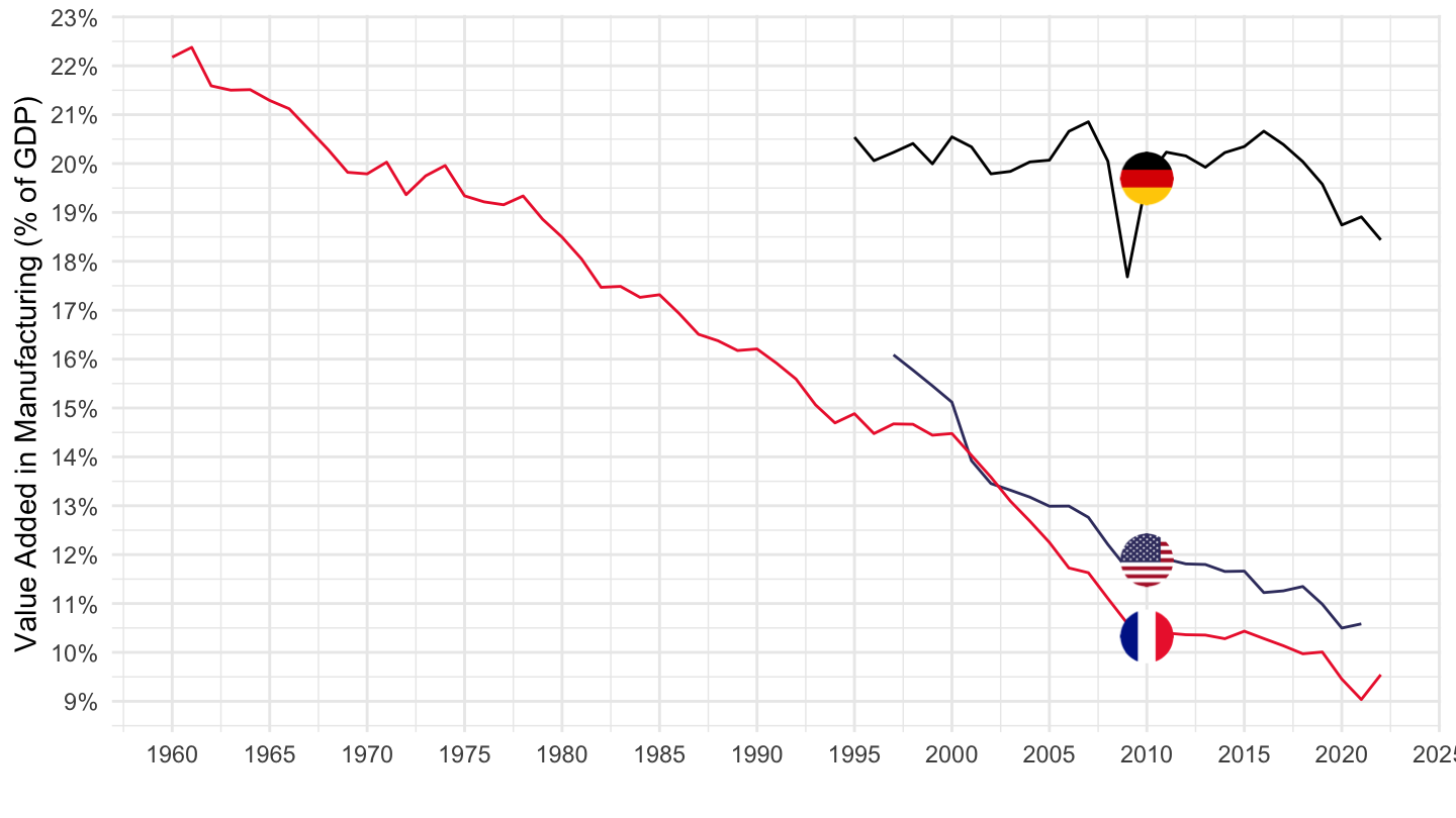

Denmark, Switzerland, UK

Code

SNA_TABLE6A |>
  filter(TRANSACT %in% c("B1GA", "B1_GE"),
         ACTIVITY %in% c("VC", "VTOT"),
         LOCATION %in% c("GBR", "DNK", "CHE"),
         MEASURE == "C") |>
  left_join(SNA_TABLE6A_var$LOCATION, by = "LOCATION") |>
  year_to_date() |>
  mutate(VARIABLE = paste0(TRANSACT, "_", ACTIVITY)) |>
  select(VARIABLE, Location, date, obsValue) |>
  spread(VARIABLE, obsValue) |>
  mutate(obsValue = B1GA_VC / B1_GE_VTOT) |>
  na.omit() |>
  add_flag_color("Location") |>
  ggplot() + geom_line(aes(x = date, y = obsValue, color = color)) + 
  scale_color_identity() + add_3flags + theme_minimal() +
  scale_x_date(breaks = seq(1920, 2100, 5) |> paste0("-01-01") |> as.Date(),
               labels = date_format("%Y")) +
  scale_y_continuous(breaks = 0.01*seq(-7, 26, 1),
                     labels = scales::percent_format(accuracy = 1)) +
  ylab("Value Added in Manufacturing (% of GDP)") + xlab("")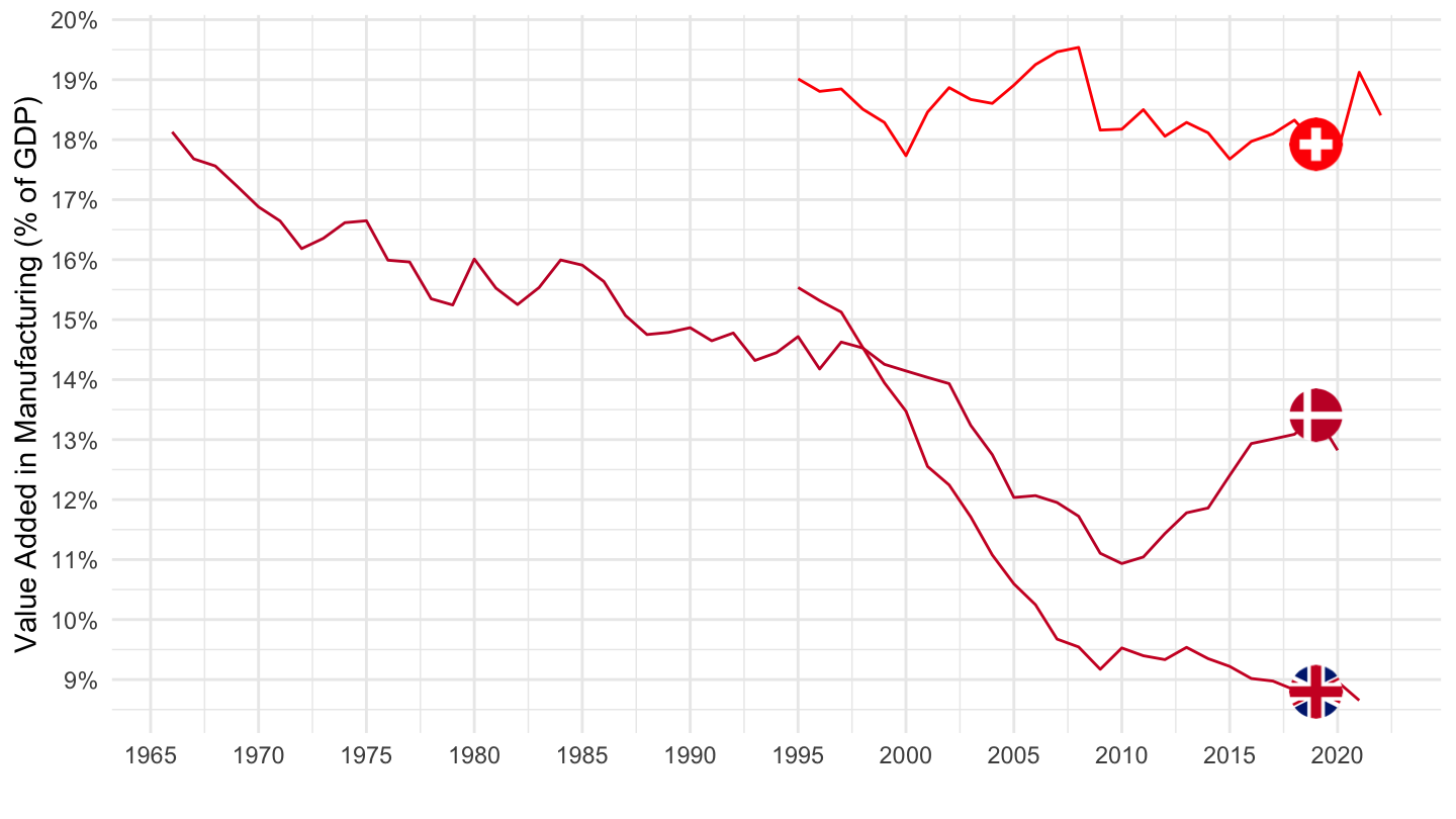

Spain, Italy, Portugal

Code

SNA_TABLE6A |>
  filter(TRANSACT %in% c("B1GA", "B1_GE"),
         ACTIVITY %in% c("VC", "VTOT"),
         LOCATION %in% c("PRT", "ESP", "ITA"),
         MEASURE == "C") |>
  left_join(SNA_TABLE6A_var$LOCATION, by = "LOCATION") |>
  year_to_date() |>
  mutate(VARIABLE = paste0(TRANSACT, "_", ACTIVITY)) |>
  select(VARIABLE, Location, date, obsValue) |>
  spread(VARIABLE, obsValue) |>
  mutate(obsValue = B1GA_VC / B1_GE_VTOT) |>
  na.omit() |>
  add_flag_color("Location") |>
  ggplot() + geom_line(aes(x = date, y = obsValue, color = color)) + 
  scale_color_identity() + add_3flags + theme_minimal() +
  scale_x_date(breaks = seq(1920, 2100, 2) |> paste0("-01-01") |> as.Date(),
               labels = date_format("%Y")) +
  scale_y_continuous(breaks = 0.01*seq(-7, 26, 1),
                     labels = scales::percent_format(accuracy = 1)) +
  ylab("Value Added in Manufacturing (% of GDP)") + xlab("")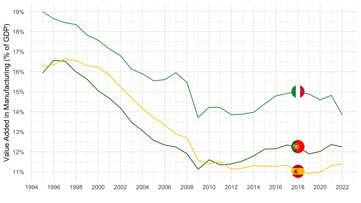

Norway, Sweden, Finland

Code

SNA_TABLE6A |>
  filter(TRANSACT %in% c("B1GA", "B1_GE"),
         ACTIVITY %in% c("VC", "VTOT"),
         LOCATION %in% c("NOR", "SWE", "FIN"),
         MEASURE == "C") |>
  left_join(SNA_TABLE6A_var$LOCATION, by = "LOCATION") |>
  year_to_date() |>
  mutate(VARIABLE = paste0(TRANSACT, "_", ACTIVITY)) |>
  select(VARIABLE, Location, date, obsValue) |>
  spread(VARIABLE, obsValue) |>
  mutate(obsValue = B1GA_VC / B1_GE_VTOT) |>
  na.omit() |>
  add_flag_color("Location") |>
  ggplot() + geom_line(aes(x = date, y = obsValue, color = color)) + 
  scale_color_identity() + add_3flags + theme_minimal() +
  scale_x_date(breaks = seq(1920, 2100, 2) |> paste0("-01-01") |> as.Date(),
               labels = date_format("%Y")) +
  scale_y_continuous(breaks = 0.01*seq(0, 40, 2),
                     labels = scales::percent_format(accuracy = 1)) +
  ylab("Value Added in Manufacturing (% of GDP)") + xlab("")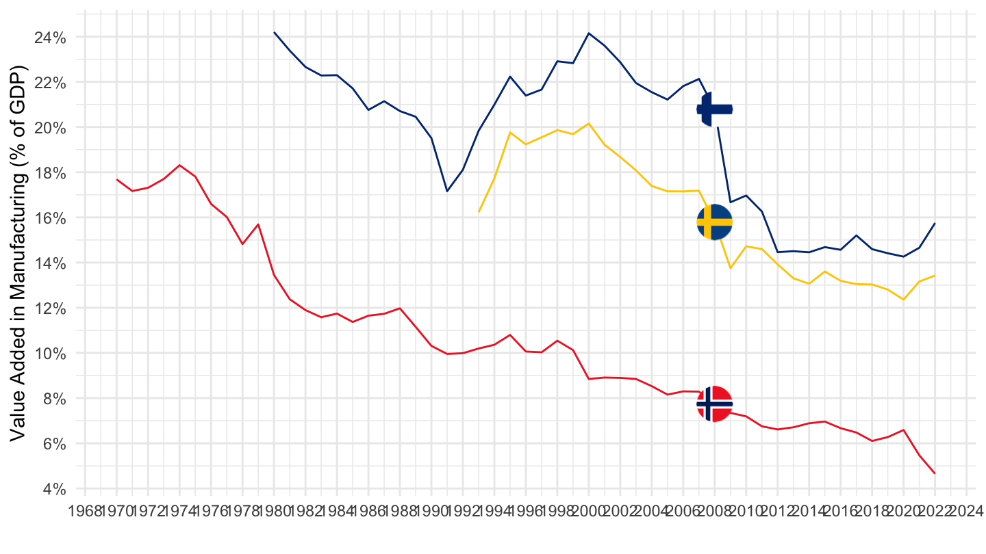

South Korea, Australia, New Zealand

Code

SNA_TABLE6A |>
  filter(TRANSACT %in% c("B1GA", "B1_GE"),
         ACTIVITY %in% c("VC", "VTOT"),
         LOCATION %in% c("KOR", "NZL", "AUS"),
         MEASURE == "C") |>
  left_join(SNA_TABLE6A_var$LOCATION, by = "LOCATION") |>
  year_to_date() |>
  mutate(VARIABLE = paste0(TRANSACT, "_", ACTIVITY)) |>
  select(VARIABLE, Location, date, obsValue) |>
  spread(VARIABLE, obsValue) |>
  mutate(obsValue = B1GA_VC / B1_GE_VTOT) |>
  na.omit() |>
  add_flag_color("Location") |>
  ggplot() + geom_line(aes(x = date, y = obsValue, color = color)) + 
  scale_color_identity() + add_3flags + theme_minimal() +
  scale_x_date(breaks = seq(1920, 2100, 2) |> paste0("-01-01") |> as.Date(),
               labels = date_format("%Y")) +
  scale_y_continuous(breaks = 0.01*seq(0, 40, 2),
                     labels = scales::percent_format(accuracy = 1)) +
  ylab("Value Added in Manufacturing (% of GDP)") + xlab("")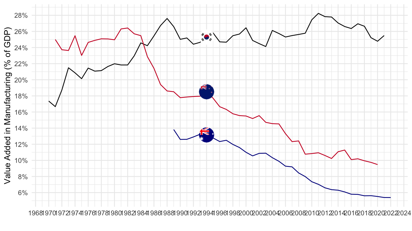

Related Data

Industry Data Overview

source	dataset	Title	Updated
oecd	SNA_TABLE6A	Value added and its components by activity, ISIC rev4 - SNA_TABLE6A	2026-08-02
ec	INDUSTRY	Industry (sector data) - INDUSTRY	2026-09-05
eurostat	nama_10_a64	National accounts aggregates by industry (up to NACE A*64) - nama_10_a64	2026-09-03
eurostat	nama_10_a64_e	National accounts employment data by industry (up to NACE A*64) - nama_10_a64_e	2026-09-04
eurostat	nama_10_gdp	GDP and main components (output, expenditure and income) - nama_10_gdp	2026-09-03
eurostat	namq_10_gdp	GDP and main components (output, expenditure and income) - namq_10_gdp	2026-09-04
eurostat	road_eqr_carmot	New registrations of passenger cars by type of motor energy and engine size - road_eqr_carmot	2026-09-03
eurostat	sts_inpr_m	Production in industry - monthly data - sts_inpr_m	2026-09-04
fred	industry	Manufacturing, Industry - industry	2026-09-01
ilo	EMP_2IND_NOC_RT_A	Industry as % of total employment – ILO modelled estimates, November 2019 - EMP_2IND_NOC_RT_A	2026-08-01
imf	DOT	Direction of Trade Statistics - DOT	2026-08-01
oecd	ALFS_EMP	Employment by activities and status (ALFS) - ALFS_EMP	2026-08-02
oecd	DP_LIVE	OECD Data Live dataset - DP_LIVE	2026-08-02
oecd	MEI_REAL	Production and Sales (MEI) - MEI_REAL	2026-08-02
oecd	MSTI_PUB	Main Science and Technology Indicators - MSTI_PUB	2026-08-02
oecd	QNA	Quarterly National Accounts - QNA	2026-09-04
oecd	QNA_manufacturing	QNA - Manufacturing - QNA_manufacturing	2026-08-02
oecd	SNA_TABLE1	Gross domestic product (GDP) - SNA_TABLE1	2026-08-02
oecd	SNA_TABLE4	PPPs and exchange rates - SNA_TABLE4	2026-08-02
oecd	SNA_TABLE6A_ARCHIVE	Value added and its components by activity, ISIC rev4, 2019 archive - SNA_TABLE6A_ARCHIVE	2026-08-02
wdi	NE.RSB.GNFS.ZS	External balance on goods and services (% of GDP) - NE.RSB.GNFS.ZS	2026-09-04
wdi	NV.IND.EMPL.KD	Industry, value added per worker (constant 2010 USD) - NV.IND.EMPL.KD	2026-09-04
wdi	NV.IND.MANF.CD	Manufacturing, value added (current USD) - NV.IND.MANF.CD	2026-09-04
wdi	NV.IND.MANF.ZS	Manufacturing, value added (% of GDP) - NV.IND.MANF.ZS	2026-09-04
wdi	NV.IND.TOTL.ZS	Industry, value added (including construction) (% of GDP) - NV.IND.TOTL.ZS	2026-09-04
wdi	PA.NUS.PPPC.RF	Price level ratio of PPP conversion factor (GDP) to market exchange rate - PA.NUS.PPPC.RF	2026-07-24
wdi	SL.IND.EMPL.ZS	Employment in industry (% of total employment) - SL.IND.EMPL.ZS	2026-09-04