Employment by A*10 industry breakdowns

Data - Eurostat

Info

Last observation: Annual: 2025 (N = 11,642)

First observation: Annual: 1975 (N = 570)

Last data update: 23 jul 2026, 23:07. Last compile: 24 jul 2026, 02:36

Structure

freq

unit

nace_r2

na_item

geo

France: Employment Share by Sector

nama_10_a10_e %>%
  filter(geo == "FR",
         nace_r2 %in% c("A", "C", "F", "G-I", "O-Q"),
         unit == "PC_TOT_PER",
         na_item == "EMP_DC") %>%
  year_to_date() %>%
  mutate(values = values/100) %>%
  ggplot + geom_line(aes(x = date, y = values, color = Nace_r2)) +
  theme_minimal() + xlab("") + ylab("Share of total employment") +
  scale_x_date(breaks = seq(1970, 2100, 5) %>% paste0("-01-01") %>% as.Date,
               labels = date_format("%Y")) +
  scale_y_continuous(labels = scales::percent_format(accuracy = 1)) +
  theme(legend.position = "right", legend.title = element_blank())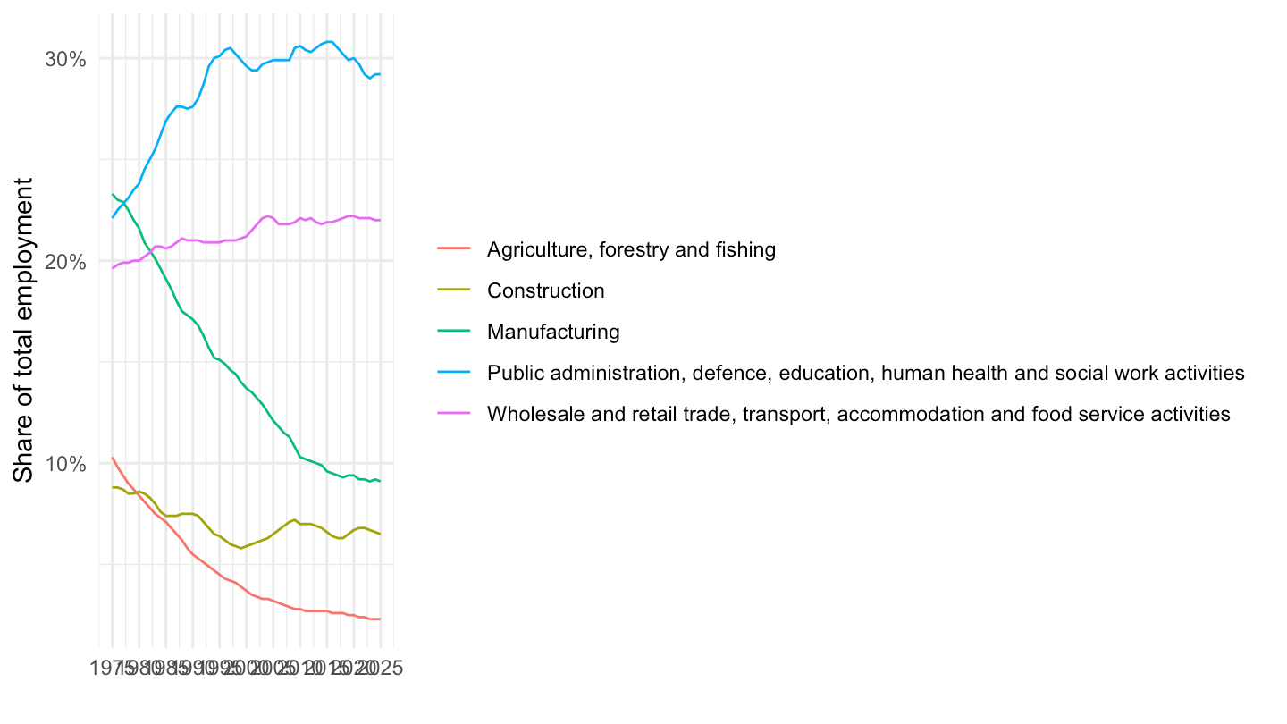

Latest Year: Employment Share by Sector and Country

latest_y <- nama_10_a10_e %>%
  filter(geo %in% c("FR", "DE", "IT"),
         unit == "PC_TOT_PER",
         na_item == "EMP_DC",
         !is.na(values)) %>%
  summarise(m = max(time)) %>%
  pull(m)

nama_10_a10_e %>%
  filter(geo %in% c("FR", "DE", "IT"),
         nace_r2 != "TOTAL",
         unit == "PC_TOT_PER",
         na_item == "EMP_DC",
         time == latest_y) %>%
  mutate(values = values/100) %>%
  select(Nace_r2, Geo, values) %>%
  spread(Geo, values) %>%
  print_table_conditional()

Nace_r2	France	Germany	Italy
Agriculture, forestry and fishing	0.023	0.012	0.035
Arts, entertainment and recreation; other service activities; activities of household and extra-territorial organizations and bodies	0.061	0.068	0.092
Construction	0.065	0.056	0.071
Financial and insurance activities	0.027	0.024	0.023
Industry (except construction)	0.101	0.172	0.160
Information and communication	0.037	0.034	0.025
Manufacturing	0.091	0.158	0.146
Professional, scientific and technical activities; administrative and support service activities	0.159	0.134	0.133
Public administration, defence, education, human health and social work activities	0.292	0.269	0.194
Real estate activities	0.013	0.011	0.007
Wholesale and retail trade, transport, accommodation and food service activities	0.220	0.219	0.260

Number of hours

nama_10_a10_e %>%
  
  filter(geo %in% c("FR", "DE", "IT"),
         nace_r2 == "C",
         unit == "THS_HW",
         na_item == "EMP_DC") %>%
  year_to_date() %>%
  arrange(date) %>%
  ggplot(.) + geom_line(aes(x = date, y = values/1000, color = geo, linetype = geo)) + 
  theme_minimal() + xlab("") + ylab("Number of Hours Worked") +
  scale_x_date(breaks = seq(1960, 2100, 5) %>% paste0("-01-01") %>% as.Date,
               labels = date_format("%Y")) +
  scale_y_continuous(breaks = seq(0, 1000000, 1000),
                     labels = dollar_format(accuracy = 1, prefix = "", suffix = "M")) +
  scale_color_manual(values = viridis(5)[1:4]) +
  theme(legend.position = c(0.2, 0.80),
        legend.title = element_blank())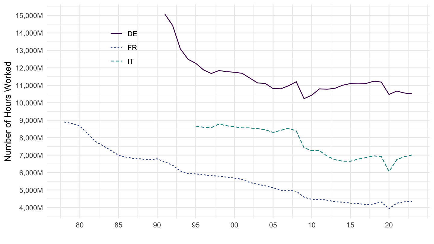

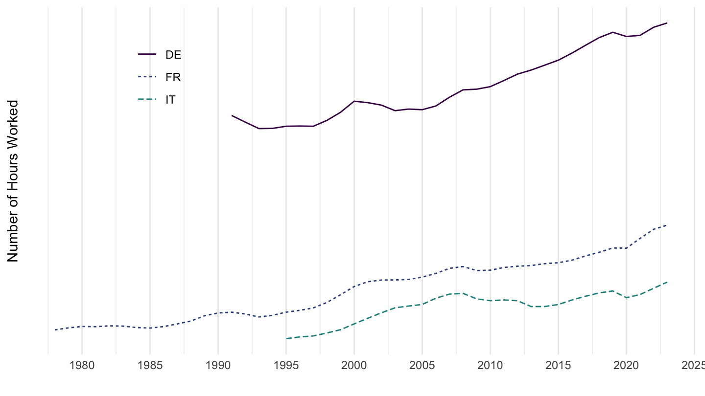
Number of hours worked

nama_10_a10_e %>%
  filter(geo %in% c("FR", "DE", "IT"),
         nace_r2 == "TOTAL",
         unit == "THS_PER",
         na_item == "EMP_DC") %>%
  year_to_date() %>%
  arrange(date) %>%
  ggplot(.) + geom_line(aes(x = date, y = values/1000, color = geo, linetype = geo)) + 
  theme_minimal() + xlab("") + ylab("Number of Hours Worked") +
  scale_x_date(breaks = seq(1960, 2100, 5) %>% paste0("-01-01") %>% as.Date,
               labels = date_format("%Y")) +
  scale_y_continuous(breaks = seq(0, 1000000, 1000),
                     labels = dollar_format(accuracy = 1, prefix = "", suffix = "M")) +
  scale_color_manual(values = viridis(5)[1:4]) +
  theme(legend.position = c(0.2, 0.80),
        legend.title = element_blank())