| source | dataset | Title | .html | .rData |
|---|---|---|---|---|
| oecd | SNA_TABLE14A | Non-financial accounts by sectors | 2026-07-23 | 2024-06-30 |
Non-financial accounts by sectors
Data - OECD
Info
Data on macro
| source | dataset | Title | .html | .rData |
|---|---|---|---|---|
| eurostat | nama_10_a10 | Gross value added and income by A*10 industry breakdowns | 2026-07-23 | 2026-07-23 |
| eurostat | nama_10_a10_e | Employment by A*10 industry breakdowns | 2026-07-23 | 2026-07-23 |
| eurostat | nama_10_gdp | GDP and main components (output, expenditure and income) | 2026-07-23 | 2026-07-23 |
| eurostat | nama_10_lp_ulc | Labour productivity and unit labour costs | 2026-07-22 | 2026-07-23 |
| eurostat | namq_10_a10 | Gross value added and income A*10 industry breakdowns | 2026-07-23 | 2026-07-23 |
| eurostat | namq_10_a10_e | Employment A*10 industry breakdowns | 2026-07-23 | 2026-07-23 |
| eurostat | namq_10_gdp | GDP and main components (output, expenditure and income) | 2026-07-23 | 2026-07-23 |
| eurostat | namq_10_lp_ulc | Labour productivity and unit labour costs | 2026-07-23 | 2026-07-23 |
| eurostat | namq_10_pc | Main GDP aggregates per capita | 2026-07-23 | 2026-07-23 |
| eurostat | nasa_10_nf_tr | Non-financial transactions | 2026-07-22 | 2026-07-23 |
| eurostat | nasq_10_nf_tr | Non-financial transactions | 2026-07-22 | 2026-07-23 |
| fred | gdp | Gross Domestic Product | 2026-07-22 | 2026-07-22 |
| oecd | QNA | Quarterly National Accounts | 2026-07-23 | 2026-07-22 |
| oecd | SNA_TABLE1 | Gross domestic product (GDP) | 2026-07-23 | 2025-05-24 |
| oecd | SNA_TABLE14A | Non-financial accounts by sectors | 2026-07-23 | 2024-06-30 |
| oecd | SNA_TABLE2 | Disposable income and net lending - net borrowing | 2024-07-01 | 2024-04-11 |
| oecd | SNA_TABLE6A | Value added and its components by activity, ISIC rev4 | 2024-07-01 | 2024-06-30 |
| wdi | NE.RSB.GNFS.ZS | External balance on goods and services (% of GDP) | 2026-07-22 | 2026-07-22 |
| wdi | NY.GDP.MKTP.CD | GDP (current USD) | 2026-07-22 | 2026-07-22 |
| wdi | NY.GDP.MKTP.PP.CD | GDP, PPP (current international D) | 2026-07-22 | 2026-07-22 |
| wdi | NY.GDP.PCAP.CD | GDP per capita (current USD) | 2026-07-22 | 2026-07-22 |
| wdi | NY.GDP.PCAP.KD | GDP per capita (constant 2015 USD) | 2026-07-22 | 2026-07-22 |
| wdi | NY.GDP.PCAP.PP.CD | GDP per capita, PPP (current international D) | 2026-02-23 | 2026-07-22 |
| wdi | NY.GDP.PCAP.PP.KD | GDP per capita, PPP (constant 2011 international D) | 2026-07-22 | 2026-07-22 |
LAST_COMPILE
| LAST_COMPILE |
|---|
| 2026-07-24 |
Last
| obsTime | Nobs |
|---|---|
| 2023 | 3 |
Sources
It presents the whole set of non financial accounts, from the production account to the acquisitions of non-financial assets accounts. For general government sector, property income, other current transfers and capital transfers are consolidated. It has been prepared from statistics reported to the OECD by Member countries in their answers to the new version of the annual national accounts questionnaire.
Layout - By Location
- OECD Website. html
United States
Code
ig_b("oecd", "SNA_TABLE14A")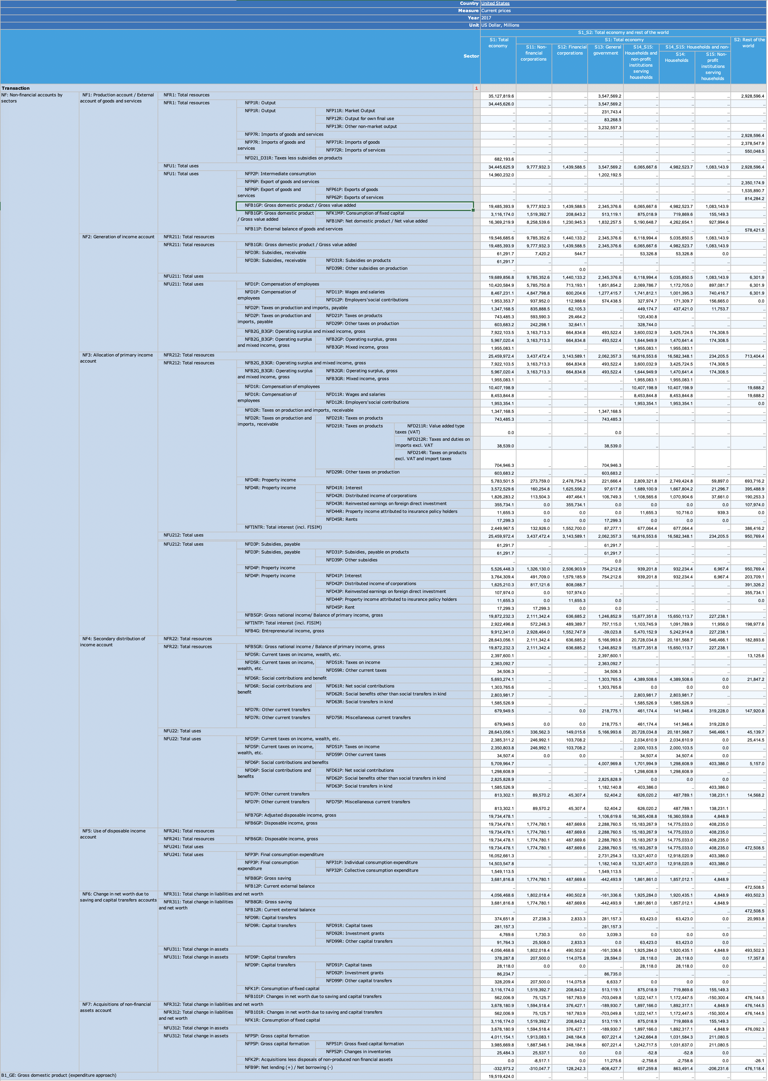
France
Code
ig_b("oecd", "SNA_TABLE14A_FRA")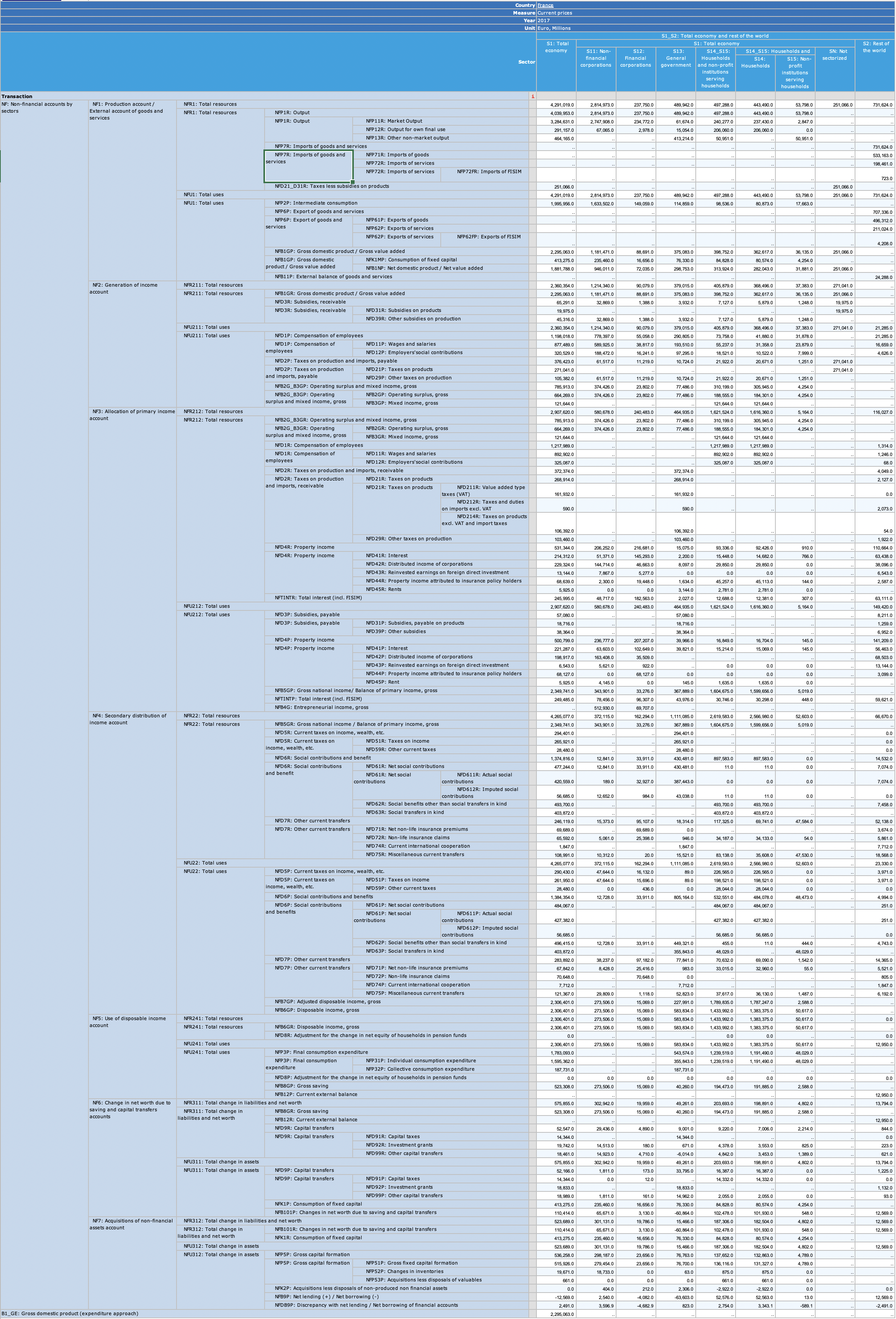
Layout - By sector
SS1 - All sectors
Code
ig_b("oecd", "SNA_TABLE14A_SS1")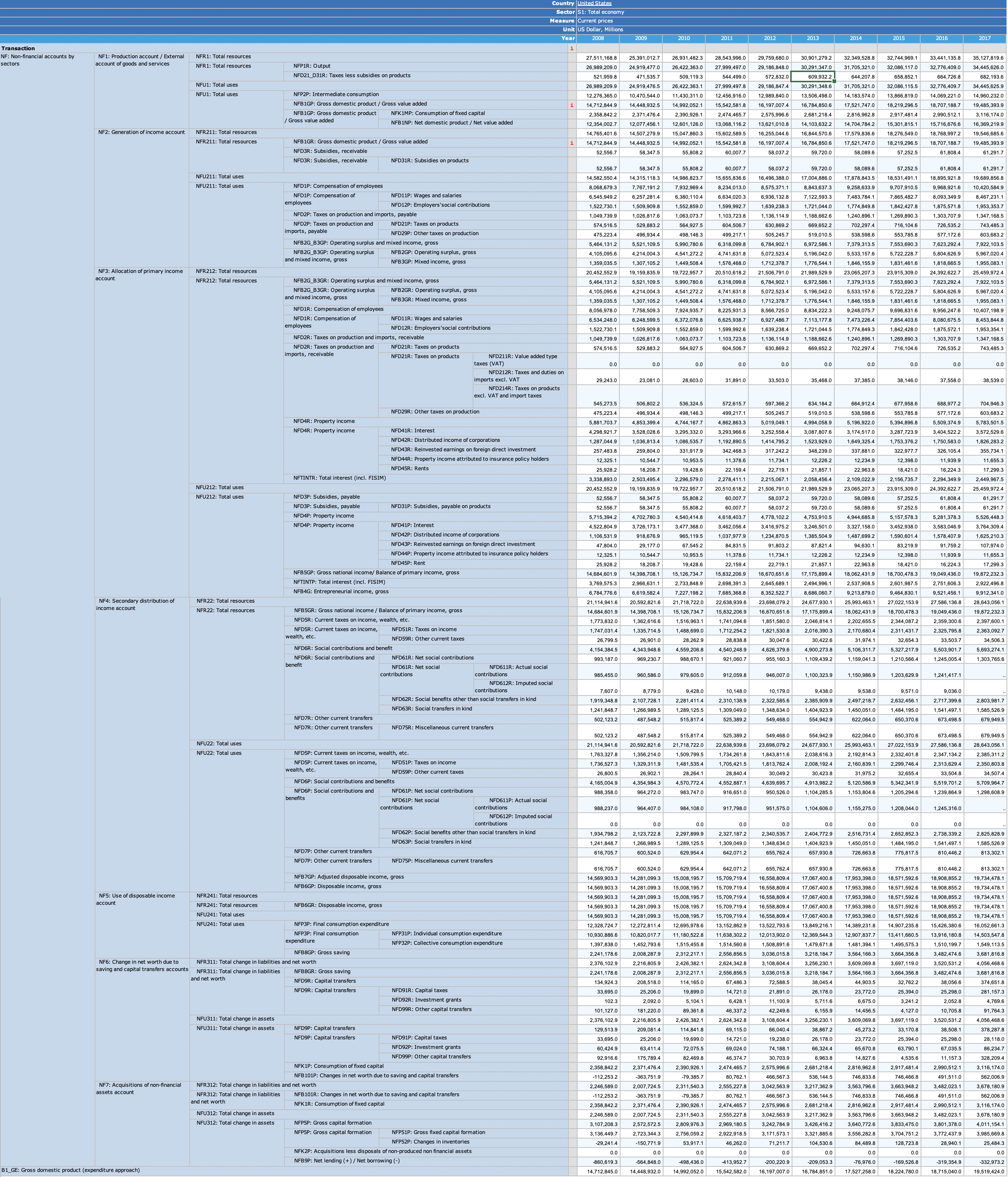
SS11 - Non-financial corporations
Code
ig_b("oecd", "SNA_TABLE14A_SS11")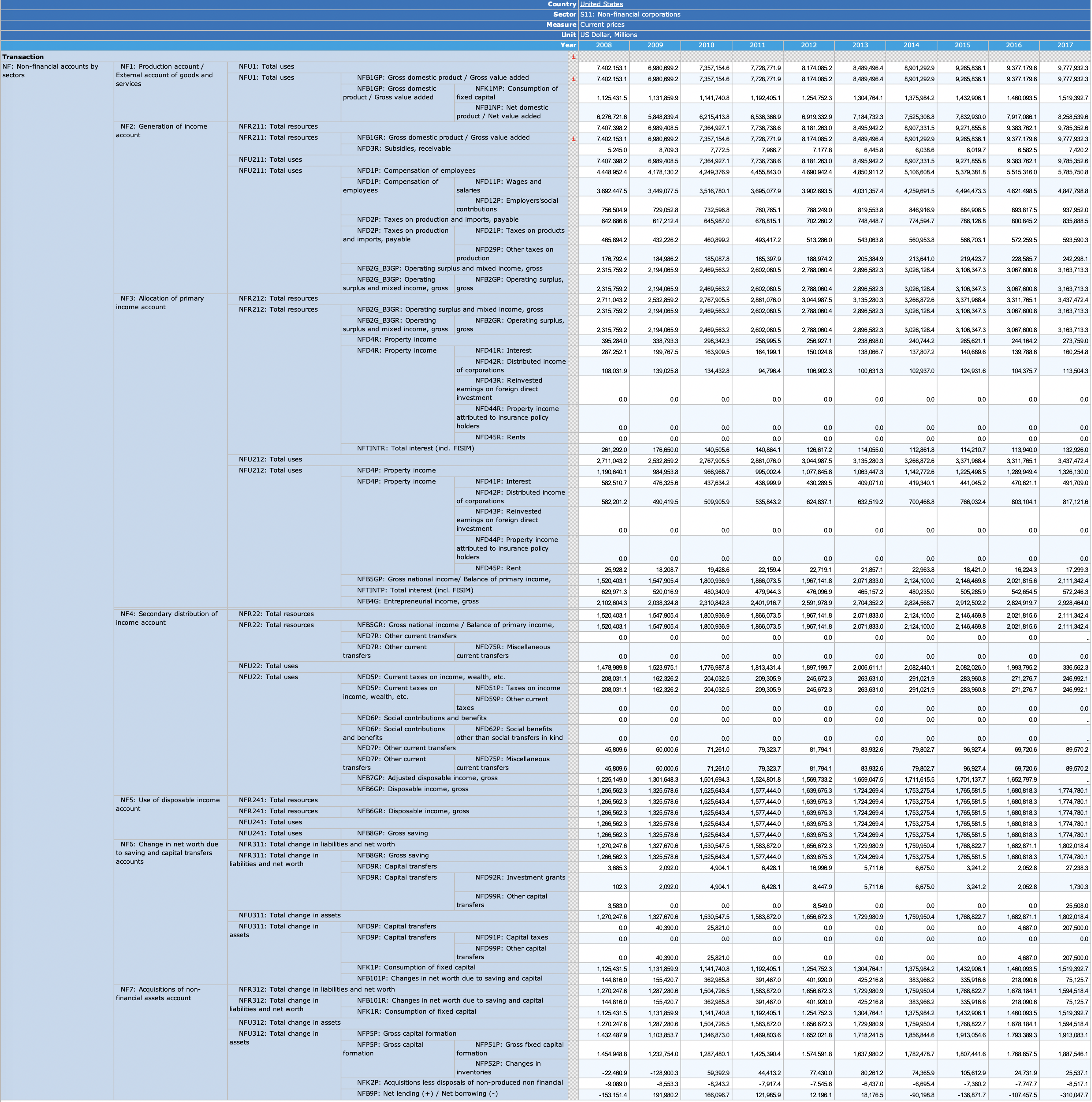
SS12 - Financial corporations
Code
ig_b("oecd", "SNA_TABLE14A_SS12")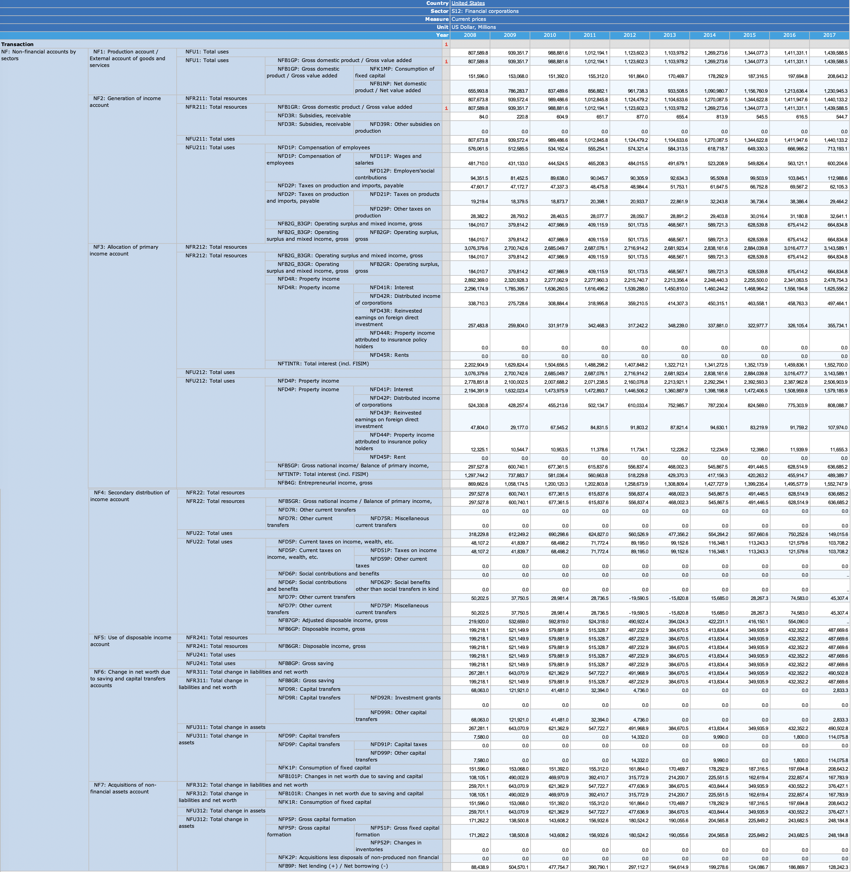
SS13 - General government
Code
ig_b("oecd", "SNA_TABLE14A_SS13")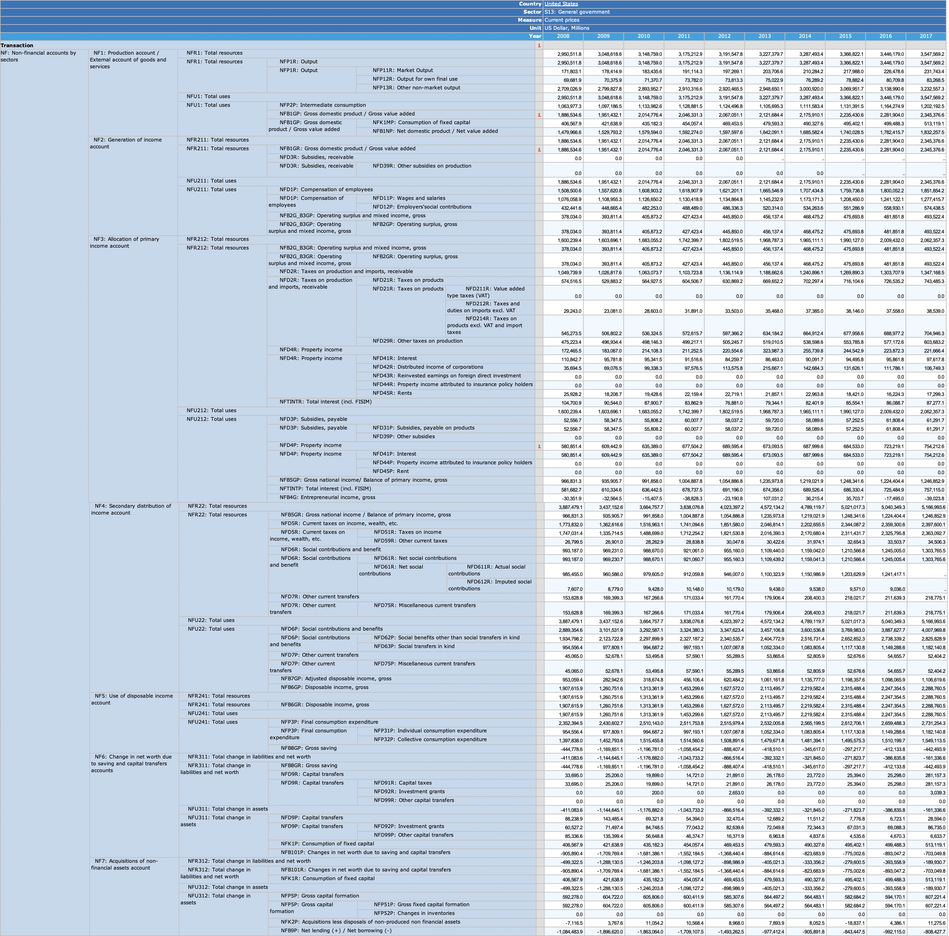
SS14_S15 - Households and Non-profits
Code
ig_b("oecd", "SNA_TABLE14A_SS14_S15")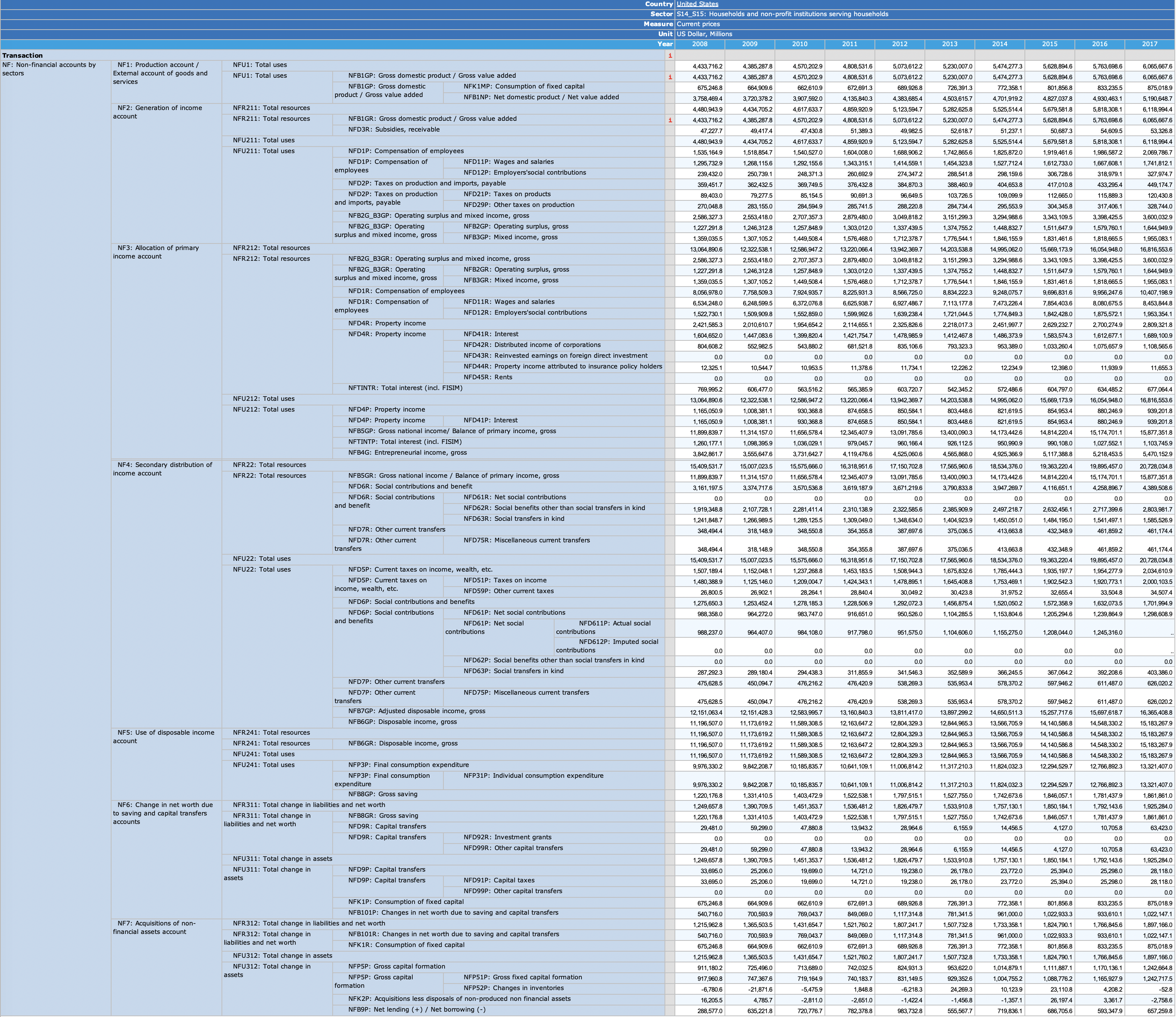
TRANSACT
Code
SNA_TABLE14A %>%
  left_join(SNA_TABLE14A_var$TRANSACT, by = "TRANSACT") %>%
  group_by(TRANSACT, Transact) %>%
  summarise(Nobs = n()) %>%
  arrange(-Nobs) %>%
  {if (is_html_output()) datatable(., filter = 'top', rownames = F) else .}
LOCATION
Code
SNA_TABLE14A %>%
  left_join(SNA_TABLE14A_var$LOCATION, by = "LOCATION") %>%
  group_by(LOCATION, Location) %>%
  summarise(Nobs = n()) %>%
  arrange(-Nobs) %>%
  mutate(Flag = gsub(" ", "-", str_to_lower(gsub(" ", "-", Location))),
         Flag = paste0('<img src="../../icon/flag/vsmall/', Flag, '.png" alt="Flag">')) %>%
  select(Flag, everything()) %>%
  {if (is_html_output()) datatable(., filter = 'top', rownames = F, escape = F) else .}
SECTOR
Code
SNA_TABLE14A_var$SECTOR %>%
{if (is_html_output()) print_table(.) else .}| SECTOR | Sector |
|---|---|
| NFAS | 14A- NFAS : NON FINANCIAL ACCOUNTS BY SECTORS |
| S1_S2 | Total economy and rest of the world |
| S1 | Total economy |
| S11 | Non-financial corporations |
| S11001 | of which: Public non-financial corporations |
| S12 | Financial corporations |
| S12001 | of which: Public financial corporations |
| S13 | General government |
| S14_S15 | Households and non-profit institutions serving households |
| S14 | Households |
| S15 | Non-profit institutions serving households |
| SN | Not sectorized |
| S2 | Rest of the world |
Saving Rate (%): NFB8GR (Gross Saving) / NFB6GR (Disposable Income, Gross)
All Sectors
Code
SNA_TABLE14A %>%
  # NFK1R: Consumption of fixed capital
  # NFP5P: Gross capital formation
  filter(TRANSACT %in% c("NFB8GR", "NFB6GR"),
         SECTOR == "S1",
         LOCATION %in% c("FRA", "USA", "DEU")) %>%
  select(LOCATION, TRANSACT, obsTime, obsValue) %>%
  spread(TRANSACT, obsValue) %>%
  left_join(SNA_TABLE14A_var$LOCATION, by = "LOCATION") %>%
  na.omit %>%
  year_to_date %>%
  mutate(obsValue = NFB8GR/NFB6GR) %>%
  filter(date >= as.Date("1995-01-01")) %>%
  left_join(colors, by = c("Location" = "country")) %>%
  mutate(color = ifelse(LOCATION == "USA", color2, color)) %>%
  ggplot() + geom_line(aes(x = date, y = obsValue, color = color)) +
  scale_color_identity() + theme_minimal() + add_3flags +
  scale_x_date(breaks = seq(1920, 2100, 2) %>% paste0("-01-01") %>% as.Date,
               labels = date_format("%Y")) +
  scale_y_continuous(breaks = 0.01*seq(-60, 60, 2),
                     labels = scales::percent_format(accuracy = 1)) +
  ylab("Gross saving rate (% of disposable income)") + xlab("")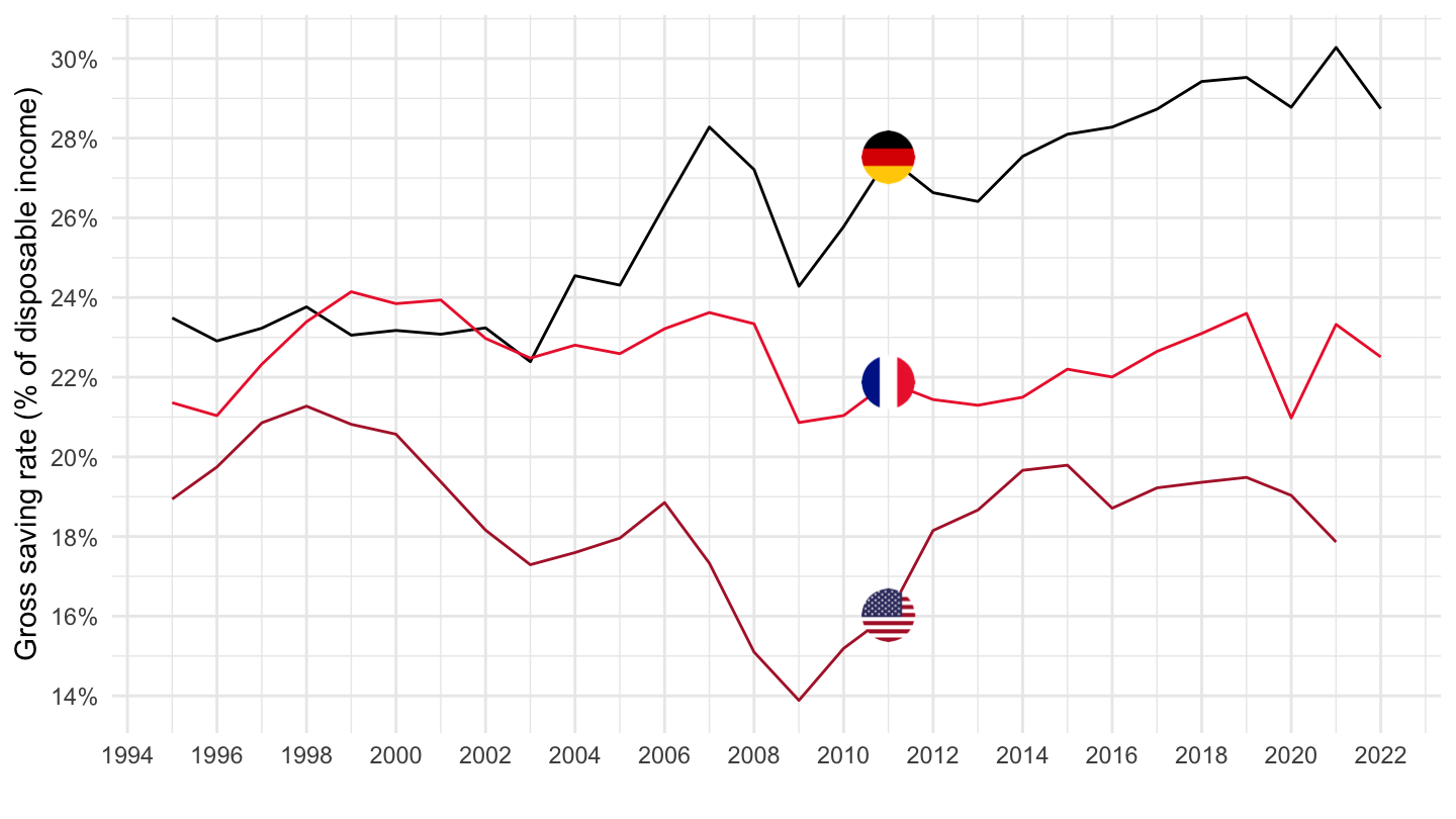
Households
Code
SNA_TABLE14A %>%
  # NFK1R: Consumption of fixed capital
  # NFP5P: Gross capital formation
  filter(TRANSACT %in% c("NFB8GR", "NFB6GR"),
         SECTOR == "S14_S15",
         LOCATION %in% c("FRA", "USA", "DEU")) %>%
  select(LOCATION, TRANSACT, obsTime, obsValue) %>%
  spread(TRANSACT, obsValue) %>%
  left_join(SNA_TABLE14A_var$LOCATION, by = "LOCATION") %>%
  na.omit %>%
  year_to_date %>%
  mutate(obsValue = NFB8GR/NFB6GR) %>%
  filter(date >= as.Date("1995-01-01")) %>%
  left_join(colors, by = c("Location" = "country")) %>%
  ggplot() + geom_line(aes(x = date, y = obsValue, color = color)) +
  scale_color_identity() + theme_minimal() + add_3flags +
  scale_x_date(breaks = seq(1920, 2100, 2) %>% paste0("-01-01") %>% as.Date,
               labels = date_format("%Y")) +
  scale_y_continuous(breaks = 0.01*seq(-60, 60, 2),
                     labels = scales::percent_format(accuracy = 1)) +
  ylab("Gross saving rate (% of disposable income)") + xlab("")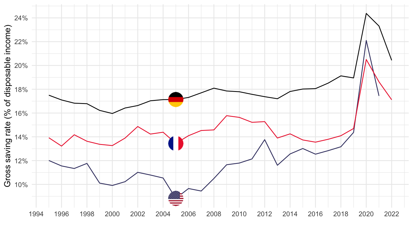
Rents (% of GDP)
France, United States, Germany
Code
SNA_TABLE14A %>%
  # NFK1R: Consumption of fixed capital
  # NFP5P: Gross capital formation
  filter(TRANSACT %in% c("NFD45R"),
         SECTOR == "S13",
         LOCATION %in% c("FRA", "USA", "DEU")) %>%
  select(LOCATION, TRANSACT, obsTime, obsValue) %>%
  spread(TRANSACT, obsValue) %>%
  left_join(SNA_TABLE1 %>%
              filter(TRANSACT == "B1_GE",
                     MEASURE == "C") %>%
              select(obsTime, LOCATION, B1_GE = obsValue),
            by = c("LOCATION", "obsTime")) %>%
  left_join(SNA_TABLE14A_var$LOCATION, by = "LOCATION") %>%
  na.omit %>%
  year_to_date %>%
  mutate(obsValue = (NFD45R) / B1_GE) %>%
  filter(date >= as.Date("1995-01-01")) %>%
  left_join(colors, by = c("Location" = "country")) %>%
  mutate(color = ifelse(LOCATION == "USA", color2, color)) %>%
  ggplot() + geom_line(aes(x = date, y = obsValue, color = color)) +
  scale_color_identity() + theme_minimal() + add_3flags +
  scale_x_date(breaks = seq(1920, 2100, 2) %>% paste0("-01-01") %>% as.Date,
               labels = date_format("%Y")) +
  scale_y_continuous(breaks = 0.01*seq(-60, 60, 0.1),
                     labels = scales::percent_format(accuracy = .1)) +
  ylab("Net Capital Formation (% of GDP) - Government") + xlab("") +
  geom_hline(yintercept = 0, linetype = "dashed")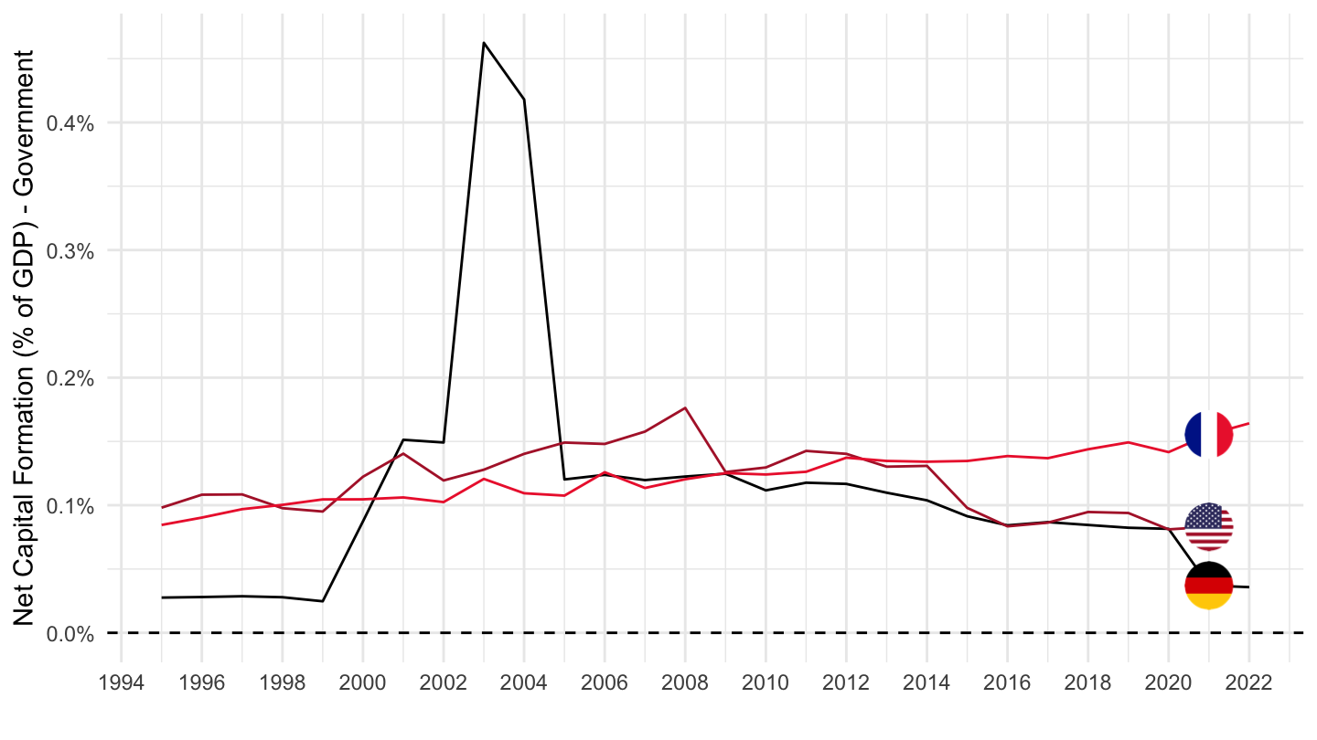
Operating surplus, Non-Financial corporations
% of Value Added
France, United States, Germany, Italy, Spain
Code
SNA_TABLE14A %>%
  # NFK1R: Consumption of fixed capital
  # NFB2GP: Operating surplus, gross
  # NFB1GP: Gross domestic product / Gross value added
  filter(TRANSACT %in% c("NFB2GP", "NFB1GP"),
         SECTOR == "S11",
         LOCATION %in% c("FRA", "USA", "DEU", "ITA", "ESP")) %>%
  select(LOCATION, TRANSACT, obsTime, obsValue) %>%
  spread(TRANSACT, obsValue) %>%
  left_join(SNA_TABLE14A_var$LOCATION, by = "LOCATION") %>%
  na.omit %>%
  year_to_date %>%
  mutate(obsValue = (NFB2GP) / NFB1GP) %>%
  left_join(colors, by = c("Location" = "country")) %>%
  ggplot() + geom_line(aes(x = date, y = obsValue, color = color)) +
  scale_color_identity() + theme_minimal() + add_5flags +
  scale_x_date(breaks = seq(1920, 2100, 5) %>% paste0("-01-01") %>% as.Date,
               labels = date_format("%Y")) +
  scale_y_continuous(breaks = 0.01*seq(-60, 60, 2),
                     labels = scales::percent_format(accuracy = 1)) +
  ylab("Net operating surplus, gross (% of GDP)") + xlab("")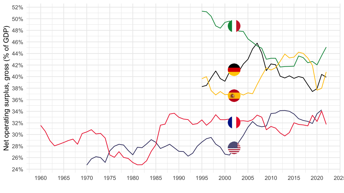
France, United States, Germany
Code
SNA_TABLE14A %>%
  # NFK1R: Consumption of fixed capital
  # NFB2GP: Operating surplus, gross
  # NFB1GP: Gross domestic product / Gross value added
  filter(TRANSACT %in% c("NFB2GP", "NFB1GP"),
         SECTOR == "S11",
         LOCATION %in% c("FRA", "USA", "DEU")) %>%
  select(LOCATION, TRANSACT, obsTime, obsValue) %>%
  spread(TRANSACT, obsValue) %>%
  left_join(SNA_TABLE14A_var$LOCATION, by = "LOCATION") %>%
  na.omit %>%
  year_to_date %>%
  mutate(obsValue = (NFB2GP) / NFB1GP) %>%
  left_join(colors, by = c("Location" = "country")) %>%
  ggplot() + geom_line(aes(x = date, y = obsValue, color = color)) +
  scale_color_identity() + theme_minimal() + add_3flags +
  scale_x_date(breaks = seq(1920, 2100, 5) %>% paste0("-01-01") %>% as.Date,
               labels = date_format("%Y")) +
  scale_y_continuous(breaks = 0.01*seq(-60, 60, 2),
                     labels = scales::percent_format(accuracy = 1)) +
  ylab("Net operating surplus, gross (% of GDP)") + xlab("")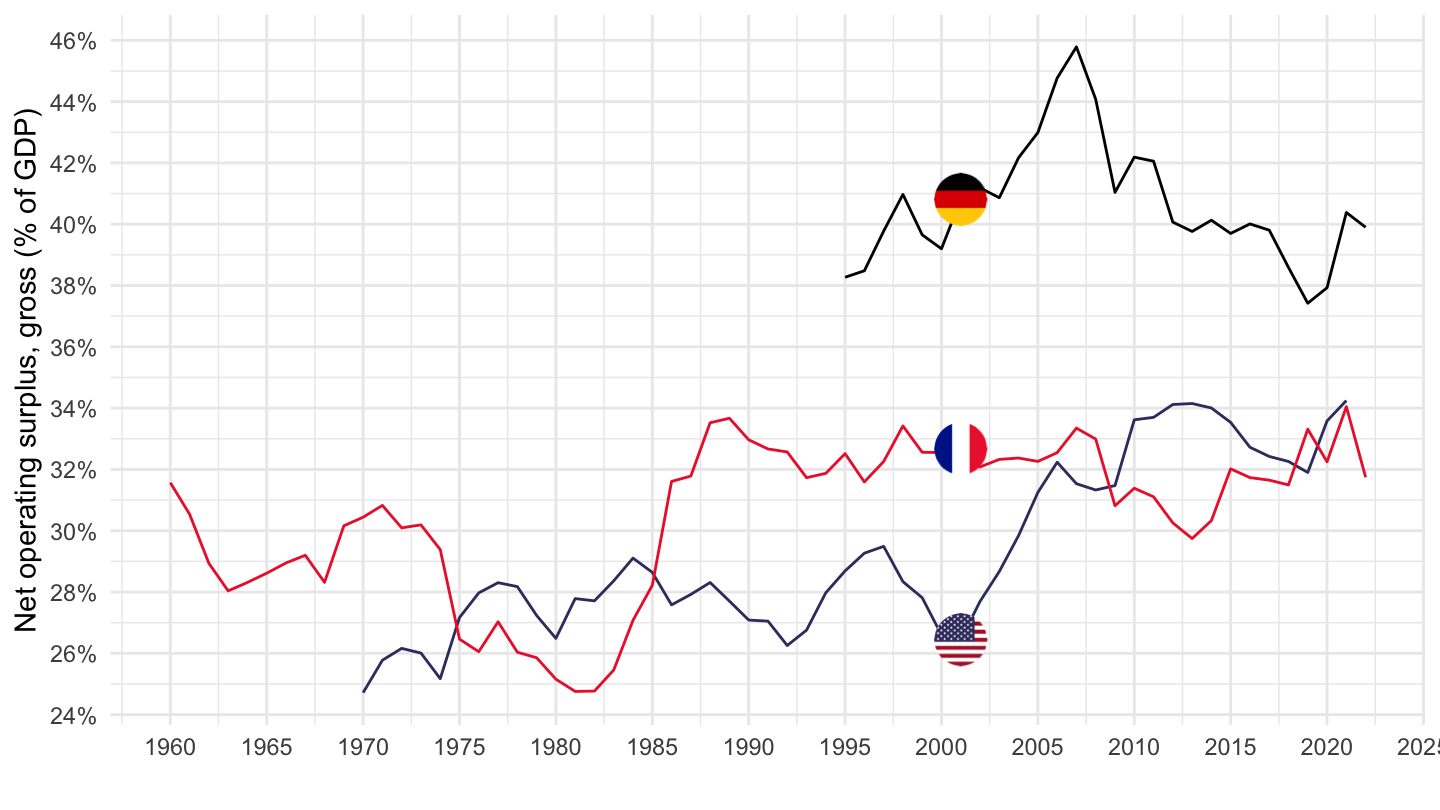
Italy, Spain, Portugal
Code
SNA_TABLE14A %>%
  # NFK1R: Consumption of fixed capital
  # NFB2GP: Operating surplus, gross
  filter(TRANSACT %in% c("NFB2GP", "NFB1GP"),
         SECTOR == "S11",
         LOCATION %in% c("ITA", "ESP", "PRT")) %>%
  select(LOCATION, TRANSACT, obsTime, obsValue) %>%
  spread(TRANSACT, obsValue) %>%
  left_join(SNA_TABLE14A_var$LOCATION, by = "LOCATION") %>%
  na.omit %>%
  year_to_date %>%
  mutate(obsValue = (NFB2GP) / NFB1GP) %>%
  left_join(colors, by = c("Location" = "country")) %>%
  mutate(color = ifelse(LOCATION == "PRT", color2, color)) %>%
  ggplot() + geom_line(aes(x = date, y = obsValue, color = color)) +
  scale_color_identity() + theme_minimal() + add_3flags +
  scale_x_date(breaks = seq(1920, 2100, 5) %>% paste0("-01-01") %>% as.Date,
               labels = date_format("%Y")) +
  scale_y_continuous(breaks = 0.01*seq(-60, 60, 2),
                     labels = scales::percent_format(accuracy = 1)) +
  ylab("Net operating surplus, gross (% of GDP)") + xlab("")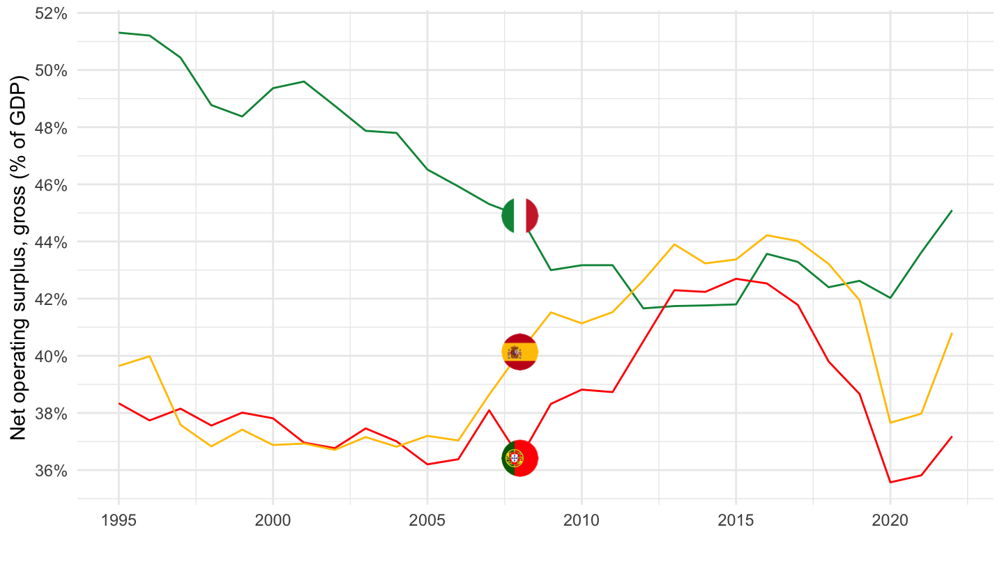
% of GDP
France, United States, Germany
Code
SNA_TABLE14A %>%
  # NFK1R: Consumption of fixed capital
  # NFB2GP: Operating surplus, gross
  # NFB1GP: Gross domestic product / Gross value added
  filter(TRANSACT %in% c("NFK1R", "NFB1GP", "NFB2GP"),
         SECTOR == "S11",
         LOCATION %in% c("FRA", "USA", "DEU")) %>%
  select(LOCATION, TRANSACT, obsTime, obsValue) %>%
  spread(TRANSACT, obsValue) %>%
  left_join(SNA_TABLE1 %>%
              filter(TRANSACT == "B1_GE",
                     MEASURE == "C") %>%
              select(obsTime, LOCATION, B1_GE = obsValue),
            by = c("LOCATION", "obsTime")) %>%
  left_join(SNA_TABLE14A_var$LOCATION, by = "LOCATION") %>%
  na.omit %>%
  year_to_date %>%
  mutate(obsValue = (NFB2GP) / B1_GE) %>%
  left_join(colors, by = c("Location" = "country")) %>%
  ggplot() + geom_line(aes(x = date, y = obsValue, color = color)) +
  scale_color_identity() + theme_minimal() + add_3flags +
  scale_x_date(breaks = seq(1920, 2100, 5) %>% paste0("-01-01") %>% as.Date,
               labels = date_format("%Y")) +
  scale_y_continuous(breaks = 0.01*seq(-60, 60, 2),
                     labels = scales::percent_format(accuracy = 1)) +
  ylab("Net operating surplus, gross (% of GDP)") + xlab("")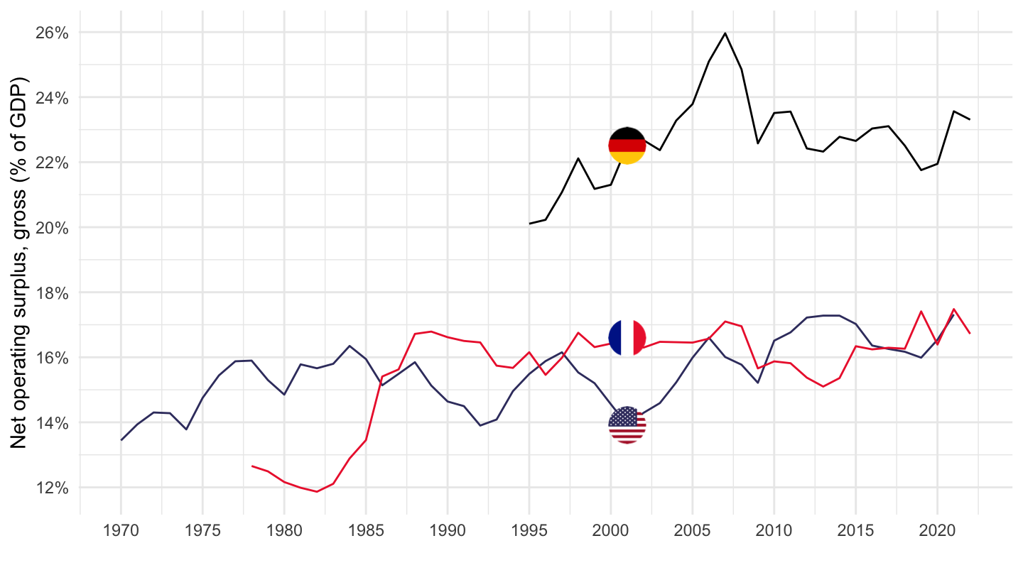
Italy, Spain, Portugal
Code
SNA_TABLE14A %>%
  # NFK1R: Consumption of fixed capital
  # NFB2GP: Operating surplus, gross
  filter(TRANSACT %in% c("NFK1R", "NFB2GP"),
         SECTOR == "S1",
         LOCATION %in% c("ITA", "ESP", "PRT")) %>%
  select(LOCATION, TRANSACT, obsTime, obsValue) %>%
  spread(TRANSACT, obsValue) %>%
  left_join(SNA_TABLE1 %>%
              filter(TRANSACT == "B1_GE",
                     MEASURE == "C") %>%
              select(obsTime, LOCATION, B1_GE = obsValue),
            by = c("LOCATION", "obsTime")) %>%
  left_join(SNA_TABLE14A_var$LOCATION, by = "LOCATION") %>%
  na.omit %>%
  year_to_date %>%
  mutate(obsValue = (NFB2GP) / B1_GE) %>%
  left_join(colors, by = c("Location" = "country")) %>%
  mutate(color = ifelse(LOCATION == "PRT", color2, color)) %>%
  ggplot() + geom_line(aes(x = date, y = obsValue, color = color)) +
  scale_color_identity() + theme_minimal() + add_3flags +
  scale_x_date(breaks = seq(1920, 2100, 5) %>% paste0("-01-01") %>% as.Date,
               labels = date_format("%Y")) +
  scale_y_continuous(breaks = 0.01*seq(-60, 60, 2),
                     labels = scales::percent_format(accuracy = 1)) +
  ylab("Net operating surplus, gross (% of GDP)") + xlab("")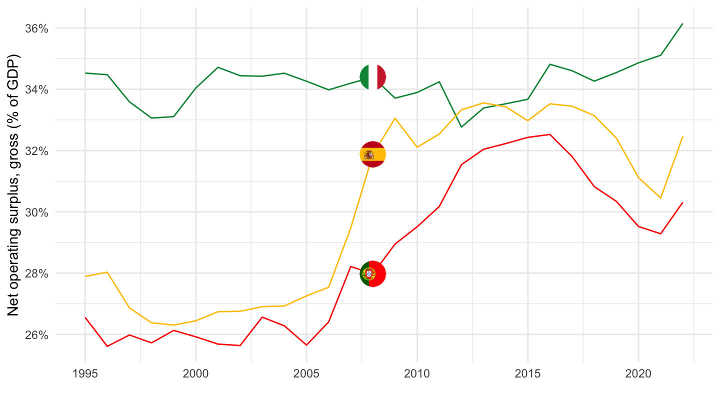
Operating surplus, gross (% of GDP) - All Economy
France, United States, Germany
Code
SNA_TABLE14A %>%
  # NFK1R: Consumption of fixed capital
  # NFB2GP: Operating surplus, gross
  filter(TRANSACT %in% c("NFK1R", "NFB2GP"),
         SECTOR == "S1",
         LOCATION %in% c("FRA", "USA", "DEU")) %>%
  select(LOCATION, TRANSACT, obsTime, obsValue) %>%
  spread(TRANSACT, obsValue) %>%
  left_join(SNA_TABLE1 %>%
              filter(TRANSACT == "B1_GE",
                     MEASURE == "C") %>%
              select(obsTime, LOCATION, B1_GE = obsValue),
            by = c("LOCATION", "obsTime")) %>%
  left_join(SNA_TABLE14A_var$LOCATION, by = "LOCATION") %>%
  na.omit %>%
  year_to_date %>%
  mutate(obsValue = (NFB2GP) / B1_GE) %>%
  left_join(colors, by = c("Location" = "country")) %>%
  mutate(color = ifelse(LOCATION == "USA", color2, color)) %>%
  ggplot() + geom_line(aes(x = date, y = obsValue, color = color)) +
  scale_color_identity() + theme_minimal() + add_3flags +
  scale_x_date(breaks = seq(1920, 2100, 5) %>% paste0("-01-01") %>% as.Date,
               labels = date_format("%Y")) +
  scale_y_continuous(breaks = 0.01*seq(-60, 60, 2),
                     labels = scales::percent_format(accuracy = 1)) +
  ylab("Net operating surplus, gross (% of GDP)") + xlab("")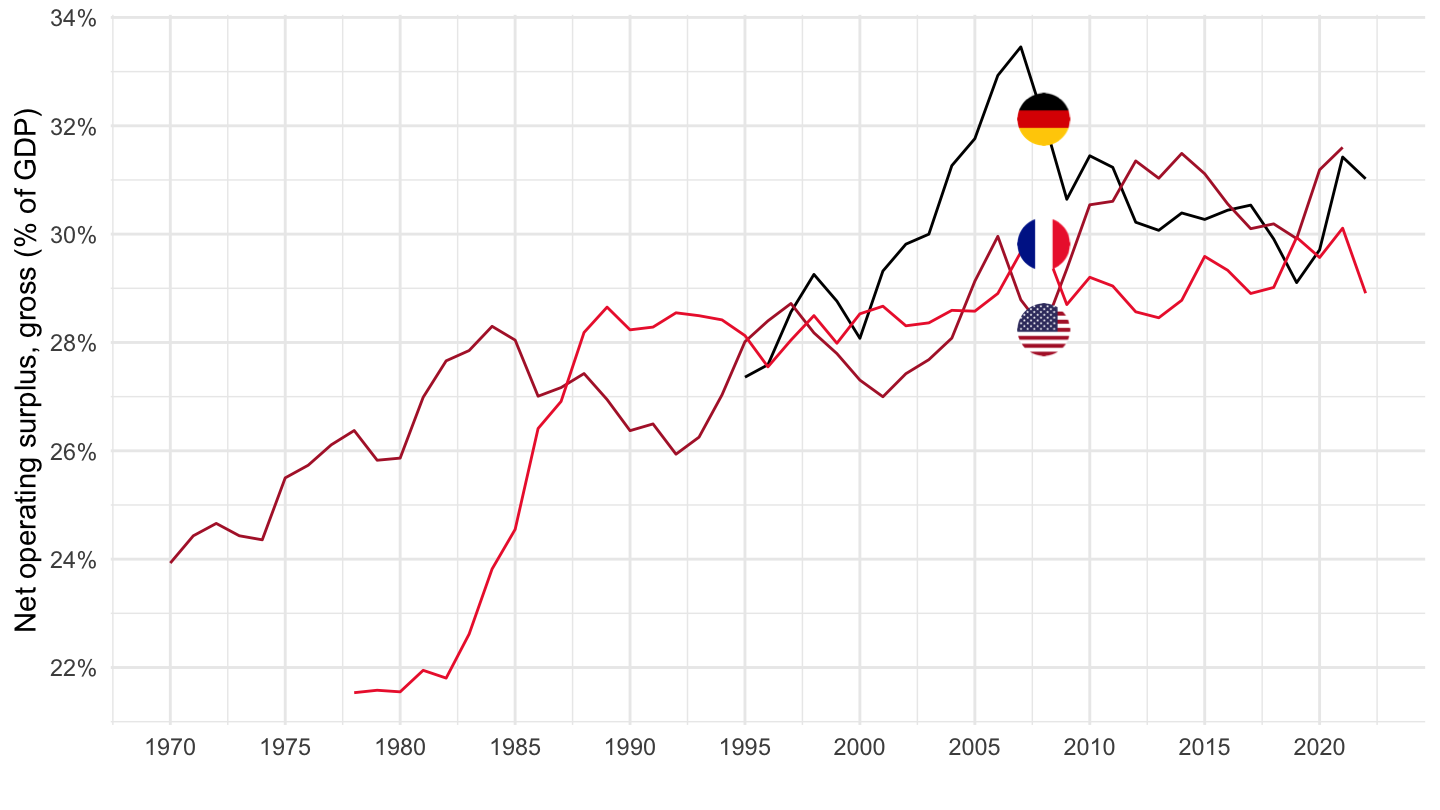
Italy, Spain, Portugal
Code
SNA_TABLE14A %>%
  # NFK1R: Consumption of fixed capital
  # NFB2GP: Operating surplus, gross
  filter(TRANSACT %in% c("NFK1R", "NFB2GP"),
         SECTOR == "S1",
         LOCATION %in% c("ITA", "ESP", "PRT")) %>%
  select(LOCATION, TRANSACT, obsTime, obsValue) %>%
  spread(TRANSACT, obsValue) %>%
  left_join(SNA_TABLE1 %>%
              filter(TRANSACT == "B1_GE",
                     MEASURE == "C") %>%
              select(obsTime, LOCATION, B1_GE = obsValue),
            by = c("LOCATION", "obsTime")) %>%
  left_join(SNA_TABLE14A_var$LOCATION, by = "LOCATION") %>%
  na.omit %>%
  year_to_date %>%
  mutate(obsValue = (NFB2GP) / B1_GE) %>%
  left_join(colors, by = c("Location" = "country")) %>%
  mutate(color = ifelse(LOCATION == "PRT", color2, color)) %>%
  ggplot() + geom_line(aes(x = date, y = obsValue, color = color)) +
  scale_color_identity() + theme_minimal() + add_3flags +
  scale_x_date(breaks = seq(1920, 2100, 5) %>% paste0("-01-01") %>% as.Date,
               labels = date_format("%Y")) +
  scale_y_continuous(breaks = 0.01*seq(-60, 60, 2),
                     labels = scales::percent_format(accuracy = 1)) +
  ylab("Net operating surplus, gross (% of GDP)") + xlab("")
Gross saving - investment (% of GDP) - NFB8GP-NFP5P
Germany
Code
SNA_TABLE14A %>%
  # NFK1R: Consumption of fixed capital
  # NFP5P: Gross capital formation
  filter(TRANSACT %in% c("NFB8GP", "NFP5P"),
         SECTOR %in% c("S1", "S11", "S13", "S14_S15"),
         LOCATION %in% c("DEU")) %>%
  select(SECTOR, LOCATION, TRANSACT, obsTime, obsValue) %>%
  spread(TRANSACT, obsValue) %>%
  left_join(SNA_TABLE1 %>%
              filter(TRANSACT == "B1_GE",
                     MEASURE == "C") %>%
              select(obsTime, LOCATION, B1_GE = obsValue),
            by = c("LOCATION", "obsTime")) %>%
  left_join(SNA_TABLE14A_var$SECTOR, by = "SECTOR") %>%
  na.omit %>%
  year_to_date %>%
  mutate(obsValue = (NFB8GP - NFP5P) / B1_GE) %>%
  ggplot() + geom_line(aes(x = date, y = obsValue, color = Sector)) +
  theme_minimal() + ylab("Gross Saving - Investment (% of GDP)") + xlab("") +
  scale_x_date(breaks = seq(1920, 2100, 5) %>% paste0("-01-01") %>% as.Date,
               labels = date_format("%Y")) +

  theme(legend.position = c(0.3, 0.9),
        legend.title = element_blank()) +
  scale_y_continuous(breaks = 0.01*seq(-60, 60, 2),
labels = scales::percent_format(accuracy = 1)) 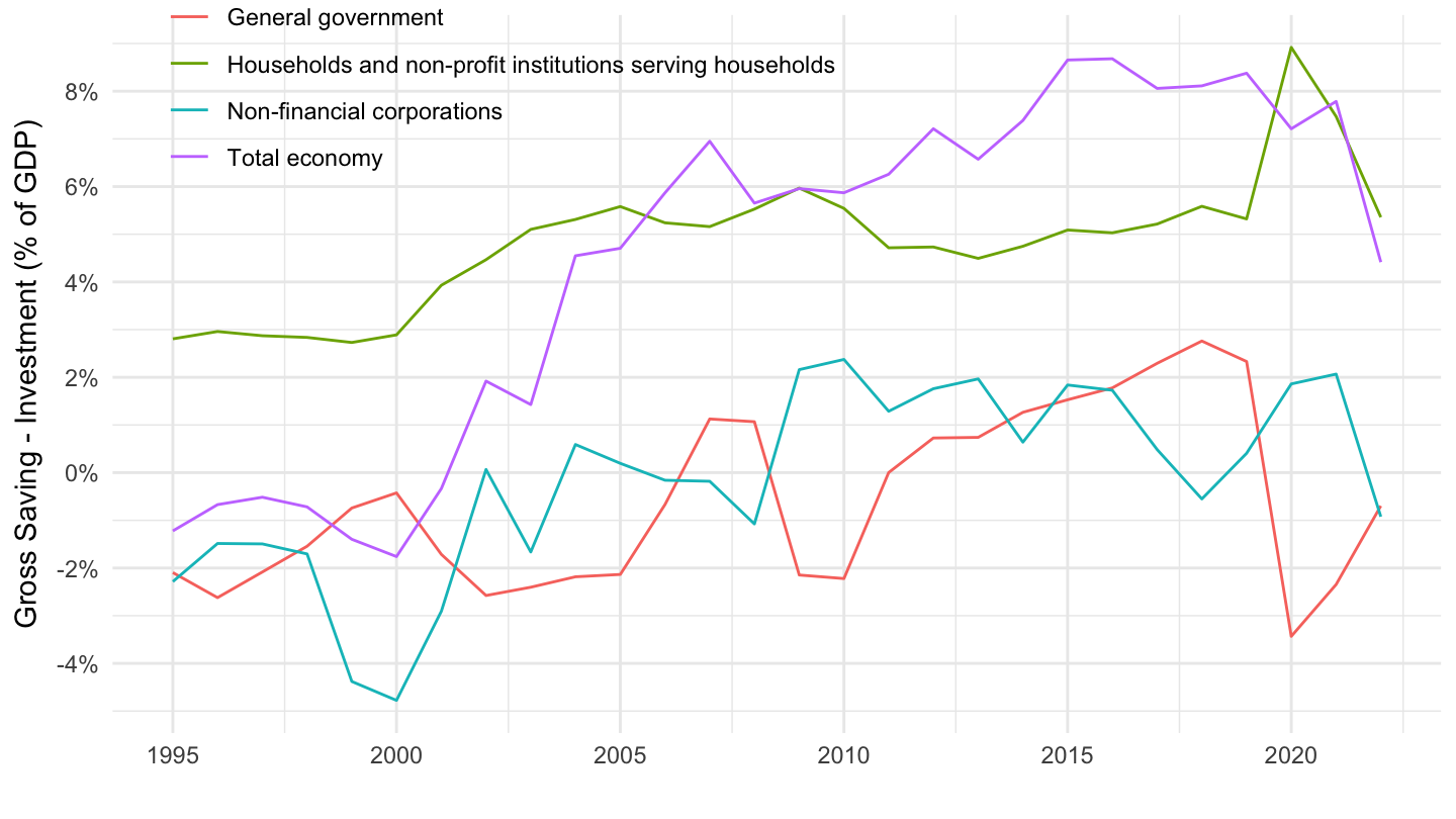
France
Code
SNA_TABLE14A %>%
  # NFK1R: Consumption of fixed capital
  # NFP5P: Gross capital formation
  filter(TRANSACT %in% c("NFB8GP", "NFP5P"),
         SECTOR %in% c("S1", "S11", "S13", "S14_S15"),
         LOCATION %in% c("FRA")) %>%
  select(SECTOR, LOCATION, TRANSACT, obsTime, obsValue) %>%
  spread(TRANSACT, obsValue) %>%
  left_join(SNA_TABLE1 %>%
              filter(TRANSACT == "B1_GE",
                     MEASURE == "C") %>%
              select(obsTime, LOCATION, B1_GE = obsValue),
            by = c("LOCATION", "obsTime")) %>%
  left_join(SNA_TABLE14A_var$SECTOR, by = "SECTOR") %>%
  na.omit %>%
  year_to_date %>%
  mutate(obsValue = (NFB8GP - NFP5P) / B1_GE) %>%
  ggplot() + geom_line(aes(x = date, y = obsValue, color = Sector)) +
  theme_minimal() + ylab("Gross Saving - Investment (% of GDP)") + xlab("") +
  scale_x_date(breaks = seq(1920, 2100, 5) %>% paste0("-01-01") %>% as.Date,
               labels = date_format("%Y")) +

  theme(legend.position = c(0.3, 0.9),
        legend.title = element_blank()) +
  scale_y_continuous(breaks = 0.01*seq(-60, 60, 2),
labels = scales::percent_format(accuracy = 1)) 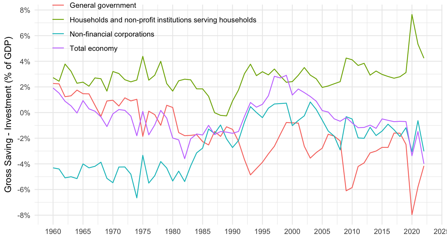
United States
Code
SNA_TABLE14A %>%
  # NFK1R: Consumption of fixed capital
  # NFP5P: Gross capital formation
  filter(TRANSACT %in% c("NFB8GP", "NFP5P"),
         SECTOR %in% c("S1", "S11", "S13", "S14_S15"),
         LOCATION %in% c("USA")) %>%
  select(SECTOR, LOCATION, TRANSACT, obsTime, obsValue) %>%
  spread(TRANSACT, obsValue) %>%
  left_join(SNA_TABLE1 %>%
              filter(TRANSACT == "B1_GE",
                     MEASURE == "C") %>%
              select(obsTime, LOCATION, B1_GE = obsValue),
            by = c("LOCATION", "obsTime")) %>%
  left_join(SNA_TABLE14A_var$SECTOR, by = "SECTOR") %>%
  na.omit %>%
  year_to_date %>%
  mutate(obsValue = (NFB8GP - NFP5P) / B1_GE) %>%
  ggplot() + geom_line(aes(x = date, y = obsValue, color = Sector)) +
  theme_minimal() + ylab("Gross Saving - Investment (% of GDP)") + xlab("") +
  scale_x_date(breaks = seq(1920, 2100, 5) %>% paste0("-01-01") %>% as.Date,
               labels = date_format("%Y")) +

  theme(legend.position = c(0.3, 0.9),
        legend.title = element_blank()) +
  scale_y_continuous(breaks = 0.01*seq(-60, 60, 2),
labels = scales::percent_format(accuracy = 1)) 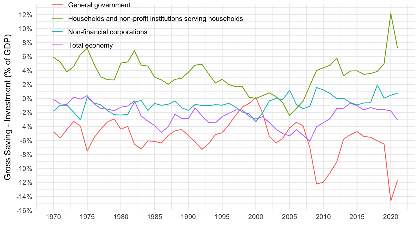
Italy
Code
SNA_TABLE14A %>%
  # NFK1R: Consumption of fixed capital
  # NFP5P: Gross capital formation
  filter(TRANSACT %in% c("NFB8GP", "NFP5P"),
         SECTOR %in% c("S1", "S11", "S13", "S14_S15"),
         LOCATION %in% c("ITA")) %>%
  select(SECTOR, LOCATION, TRANSACT, obsTime, obsValue) %>%
  spread(TRANSACT, obsValue) %>%
  left_join(SNA_TABLE1 %>%
              filter(TRANSACT == "B1_GE",
                     MEASURE == "C") %>%
              select(obsTime, LOCATION, B1_GE = obsValue),
            by = c("LOCATION", "obsTime")) %>%
  left_join(SNA_TABLE14A_var$SECTOR, by = "SECTOR") %>%
  na.omit %>%
  year_to_date %>%
  mutate(obsValue = (NFB8GP - NFP5P) / B1_GE) %>%
  ggplot() + geom_line(aes(x = date, y = obsValue, color = Sector)) +
  theme_minimal() + ylab("Gross Saving - Investment (% of GDP)") + xlab("") +
  scale_x_date(breaks = seq(1920, 2100, 5) %>% paste0("-01-01") %>% as.Date,
               labels = date_format("%Y")) +

  theme(legend.position = c(0.3, 0.9),
        legend.title = element_blank()) +
  scale_y_continuous(breaks = 0.01*seq(-60, 60, 2),
labels = scales::percent_format(accuracy = 1)) 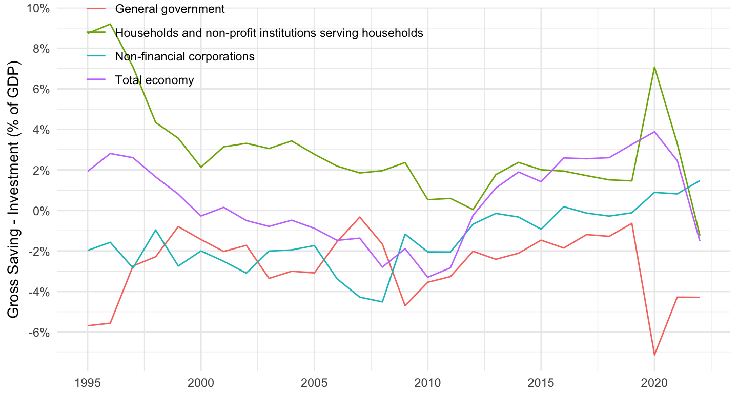
France, United States, Germany
All
Code
SNA_TABLE14A %>%
  # NFK1R: Consumption of fixed capital
  # NFP5P: Gross capital formation
  filter(TRANSACT %in% c("NFB8GP", "NFP5P"),
         SECTOR == "S1",
         LOCATION %in% c("FRA", "USA", "DEU")) %>%
  select(LOCATION, TRANSACT, obsTime, obsValue) %>%
  spread(TRANSACT, obsValue) %>%
  left_join(SNA_TABLE1 %>%
              filter(TRANSACT == "B1_GE",
                     MEASURE == "C") %>%
              select(obsTime, LOCATION, B1_GE = obsValue),
            by = c("LOCATION", "obsTime")) %>%
  left_join(SNA_TABLE14A_var$LOCATION, by = "LOCATION") %>%
  na.omit %>%
  year_to_date %>%
  mutate(obsValue = (NFB8GP - NFP5P) / B1_GE) %>%
  filter(date >= as.Date("1995-01-01")) %>%
  left_join(colors, by = c("Location" = "country")) %>%
  mutate(color = ifelse(LOCATION == "USA", color2, color)) %>%
  ggplot() + geom_line(aes(x = date, y = obsValue, color = color)) +
  scale_color_identity() + theme_minimal() + add_3flags +
  scale_x_date(breaks = seq(1920, 2100, 2) %>% paste0("-01-01") %>% as.Date,
               labels = date_format("%Y")) +
  scale_y_continuous(breaks = 0.01*seq(-60, 60, 2),
                     labels = scales::percent_format(accuracy = 1)) +
  ylab("Net Capital Formation (% of GDP) - Government") + xlab("") +
  geom_hline(yintercept = 0, linetype = "dashed")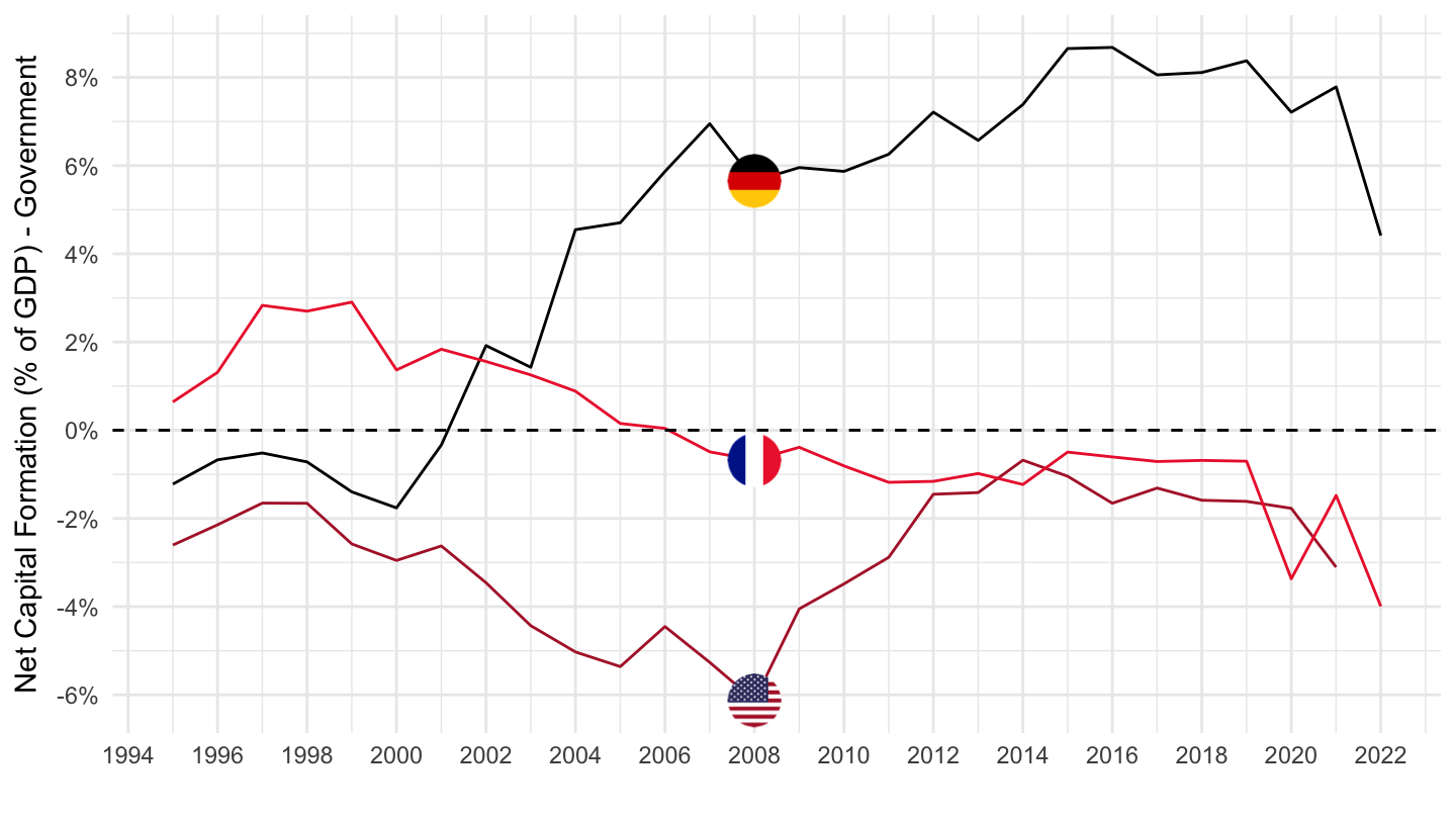
S13 - Government
Code
SNA_TABLE14A %>%
  # NFK1R: Consumption of fixed capital
  # NFP5P: Gross capital formation
  filter(TRANSACT %in% c("NFB8GP", "NFP5P"),
         SECTOR == "S13",
         LOCATION %in% c("FRA", "USA", "DEU")) %>%
  select(LOCATION, TRANSACT, obsTime, obsValue) %>%
  spread(TRANSACT, obsValue) %>%
  left_join(SNA_TABLE1 %>%
              filter(TRANSACT == "B1_GE",
                     MEASURE == "C") %>%
              select(obsTime, LOCATION, B1_GE = obsValue),
            by = c("LOCATION", "obsTime")) %>%
  left_join(SNA_TABLE14A_var$LOCATION, by = "LOCATION") %>%
  na.omit %>%
  year_to_date %>%
  mutate(obsValue = (NFB8GP - NFP5P) / B1_GE) %>%
  filter(date >= as.Date("1995-01-01")) %>%
  left_join(colors, by = c("Location" = "country")) %>%
  mutate(color = ifelse(LOCATION == "USA", color2, color)) %>%
  ggplot() + geom_line(aes(x = date, y = obsValue, color = color)) +
  scale_color_identity() + theme_minimal() + add_3flags +
  scale_x_date(breaks = seq(1920, 2100, 2) %>% paste0("-01-01") %>% as.Date,
               labels = date_format("%Y")) +
  scale_y_continuous(breaks = 0.01*seq(-60, 60, 2),
                     labels = scales::percent_format(accuracy = 1)) +
  ylab("Net Capital Formation (% of GDP) - Government") + xlab("") +
  geom_hline(yintercept = 0, linetype = "dashed")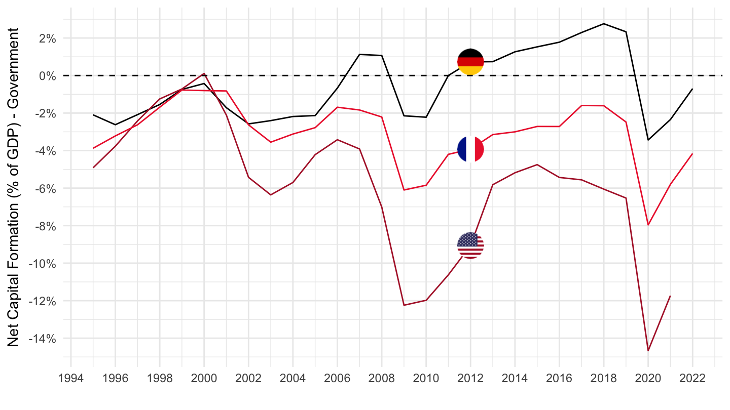
S11
Code
SNA_TABLE14A %>%
  # NFK1R: Consumption of fixed capital
  # NFP5P: Gross capital formation
  filter(TRANSACT %in% c("NFB8GP", "NFP5P"),
         SECTOR == "S11",
         LOCATION %in% c("FRA", "USA", "DEU")) %>%
  select(LOCATION, TRANSACT, obsTime, obsValue) %>%
  spread(TRANSACT, obsValue) %>%
  left_join(SNA_TABLE1 %>%
              filter(TRANSACT == "B1_GE",
                     MEASURE == "C") %>%
              select(obsTime, LOCATION, B1_GE = obsValue),
            by = c("LOCATION", "obsTime")) %>%
  left_join(SNA_TABLE14A_var$LOCATION, by = "LOCATION") %>%
  na.omit %>%
  year_to_date %>%
  mutate(obsValue = (NFB8GP - NFP5P) / B1_GE) %>%
  filter(date >= as.Date("1995-01-01")) %>%
  left_join(colors, by = c("Location" = "country")) %>%
  mutate(color = ifelse(LOCATION == "USA", color2, color)) %>%
  ggplot() + geom_line(aes(x = date, y = obsValue, color = color)) +
  scale_color_identity() + theme_minimal() + add_3flags +
  scale_x_date(breaks = seq(1920, 2100, 2) %>% paste0("-01-01") %>% as.Date,
               labels = date_format("%Y")) +
  scale_y_continuous(breaks = 0.01*seq(-60, 60, 2),
                     labels = scales::percent_format(accuracy = 1)) +
  ylab("Net Capital Formation (% of GDP) - Government") + xlab("") +
  geom_hline(yintercept = 0, linetype = "dashed")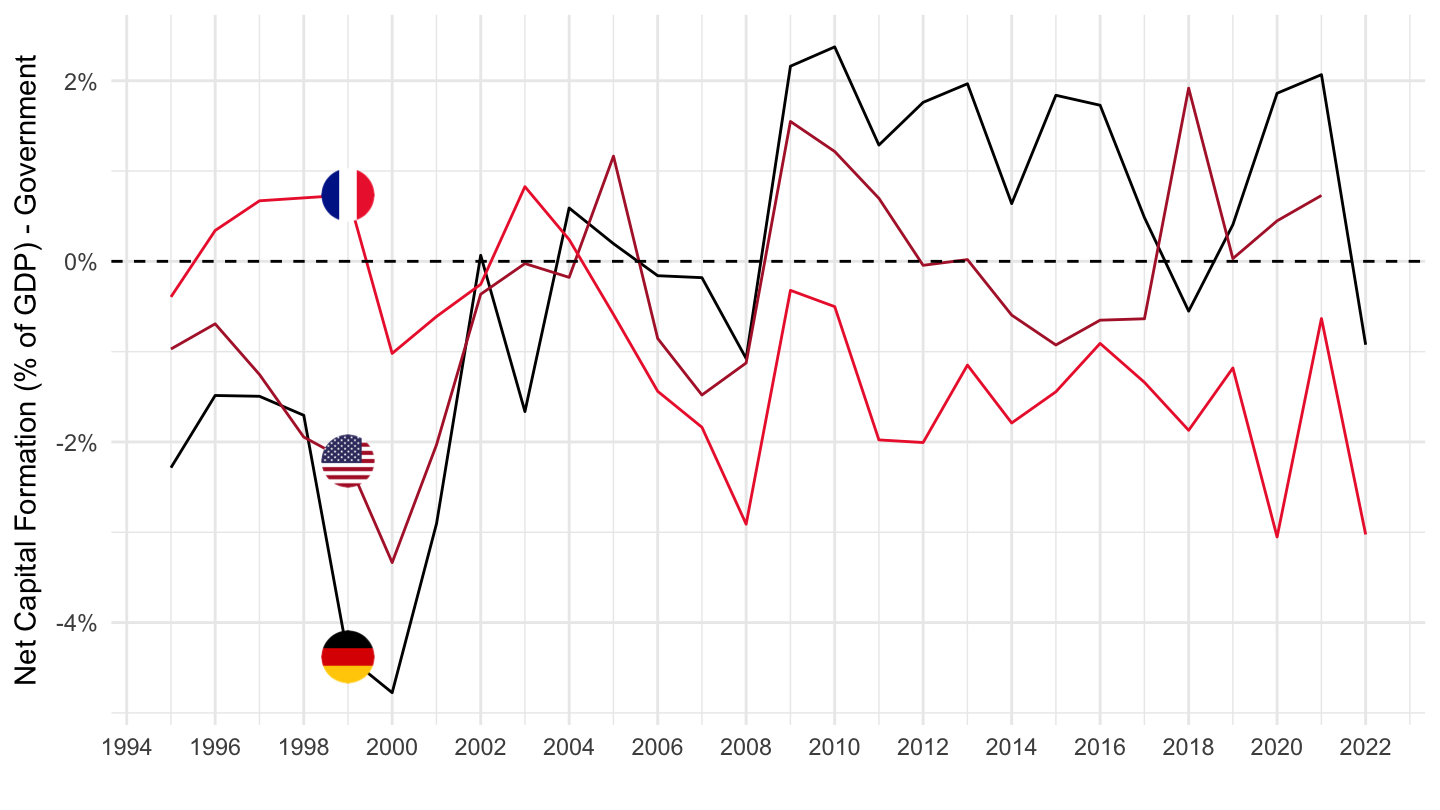
S12
Code
SNA_TABLE14A %>%
  # NFK1R: Consumption of fixed capital
  # NFP5P: Gross capital formation
  filter(TRANSACT %in% c("NFB8GP", "NFP5P"),
         SECTOR == "S12",
         LOCATION %in% c("FRA", "USA", "DEU")) %>%
  select(LOCATION, TRANSACT, obsTime, obsValue) %>%
  spread(TRANSACT, obsValue) %>%
  left_join(SNA_TABLE1 %>%
              filter(TRANSACT == "B1_GE",
                     MEASURE == "C") %>%
              select(obsTime, LOCATION, B1_GE = obsValue),
            by = c("LOCATION", "obsTime")) %>%
  left_join(SNA_TABLE14A_var$LOCATION, by = "LOCATION") %>%
  na.omit %>%
  year_to_date %>%
  mutate(obsValue = (NFB8GP - NFP5P) / B1_GE) %>%
  filter(date >= as.Date("1995-01-01")) %>%
  left_join(colors, by = c("Location" = "country")) %>%
  mutate(color = ifelse(LOCATION == "USA", color2, color)) %>%
  ggplot() + geom_line(aes(x = date, y = obsValue, color = color)) +
  scale_color_identity() + theme_minimal() + add_3flags +
  scale_x_date(breaks = seq(1920, 2100, 2) %>% paste0("-01-01") %>% as.Date,
               labels = date_format("%Y")) +
  scale_y_continuous(breaks = 0.01*seq(-60, 60, 1),
                     labels = scales::percent_format(accuracy = 1)) +
  ylab("Net Capital Formation (% of GDP) - Government") + xlab("") +
  geom_hline(yintercept = 0, linetype = "dashed")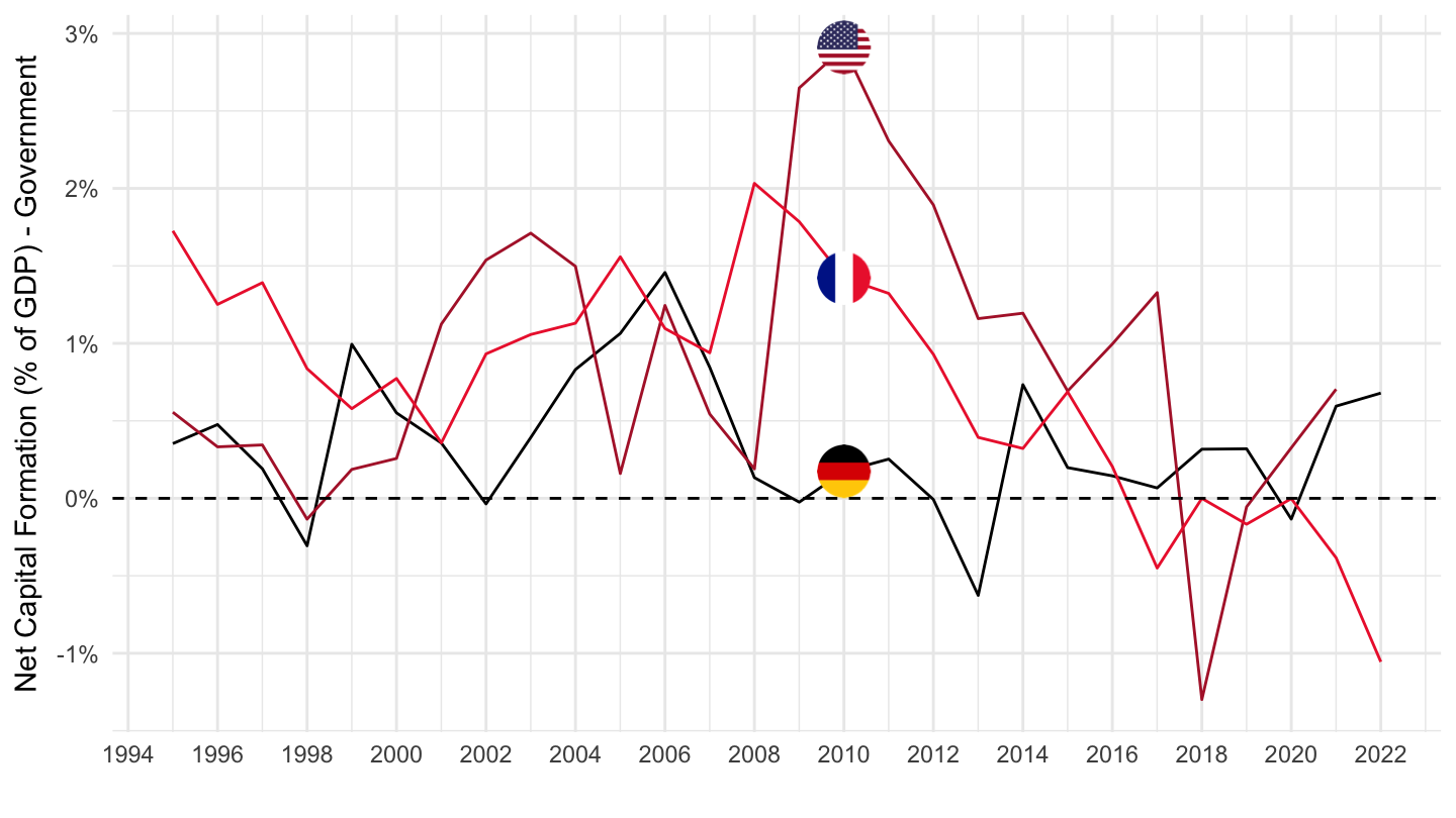
S14_S15
Code
SNA_TABLE14A %>%
  # NFK1R: Consumption of fixed capital
  # NFP5P: Gross capital formation
  filter(TRANSACT %in% c("NFB8GP", "NFP5P"),
         SECTOR == "S14_S15",
         LOCATION %in% c("FRA", "USA", "DEU")) %>%
  select(LOCATION, TRANSACT, obsTime, obsValue) %>%
  spread(TRANSACT, obsValue) %>%
  left_join(SNA_TABLE1 %>%
              filter(TRANSACT == "B1_GE",
                     MEASURE == "C") %>%
              select(obsTime, LOCATION, B1_GE = obsValue),
            by = c("LOCATION", "obsTime")) %>%
  left_join(SNA_TABLE14A_var$LOCATION, by = "LOCATION") %>%
  na.omit %>%
  year_to_date %>%
  mutate(obsValue = (NFB8GP - NFP5P) / B1_GE) %>%
  filter(date >= as.Date("1995-01-01")) %>%
  left_join(colors, by = c("Location" = "country")) %>%
  mutate(color = ifelse(LOCATION == "USA", color2, color)) %>%
  ggplot() + geom_line(aes(x = date, y = obsValue, color = color)) +
  scale_color_identity() + theme_minimal() + add_3flags +
  scale_x_date(breaks = seq(1920, 2100, 2) %>% paste0("-01-01") %>% as.Date,
               labels = date_format("%Y")) +
  scale_y_continuous(breaks = 0.01*seq(-60, 60, 1),
                     labels = scales::percent_format(accuracy = 1)) +
  ylab("Net Capital Formation (% of GDP) - Government") + xlab("") +
  geom_hline(yintercept = 0, linetype = "dashed")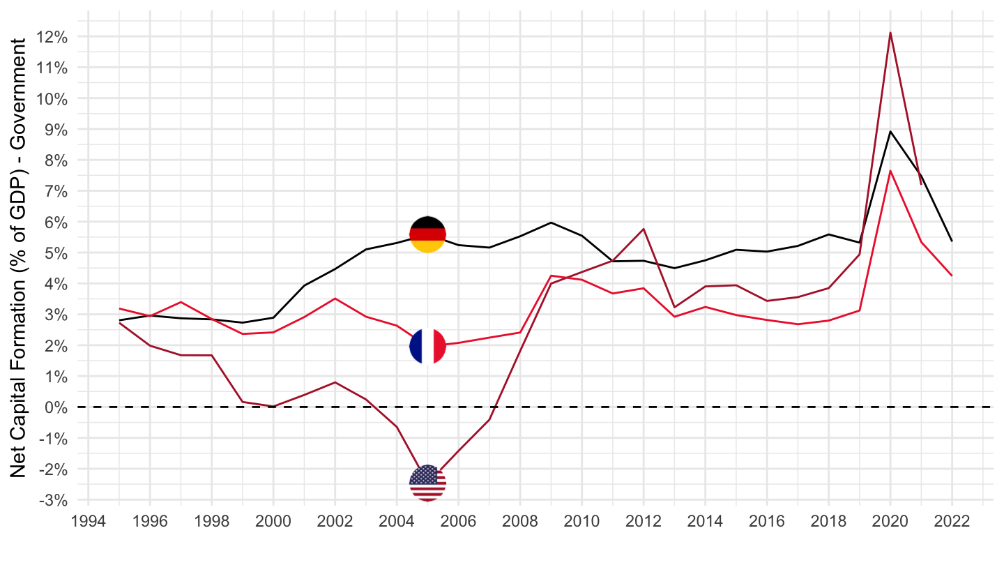
Gross saving (% of GDP)
Germany
Code
SNA_TABLE14A %>%
  # NFK1R: Consumption of fixed capital
  # NFP5P: Gross capital formation
  filter(TRANSACT %in% c("NFB8GP"),
         SECTOR %in% c("S1", "S11", "S13", "S14_S15"),
         LOCATION %in% c("DEU")) %>%
  left_join(SNA_TABLE1 %>%
              filter(TRANSACT == "B1_GE",
                     MEASURE == "C") %>%
              select(obsTime, LOCATION, B1_GE = obsValue),
            by = c("LOCATION", "obsTime")) %>%
  left_join(SNA_TABLE14A_var$SECTOR, by = "SECTOR") %>%
  mutate(obsValue = obsValue / B1_GE) %>%
  year_to_date %>%
  ggplot() + geom_line(aes(x = date, y = obsValue, color = Sector)) +
  theme_minimal() + ylab("Gross Saving (% of GDP)") + xlab("") +
  scale_x_date(breaks = seq(1920, 2100, 5) %>% paste0("-01-01") %>% as.Date,
               labels = date_format("%Y")) +

  theme(legend.position = c(0.3, 0.9),
        legend.title = element_blank()) +
  scale_y_continuous(breaks = 0.01*seq(-60, 60, 5),
labels = scales::percent_format(accuracy = 1)) 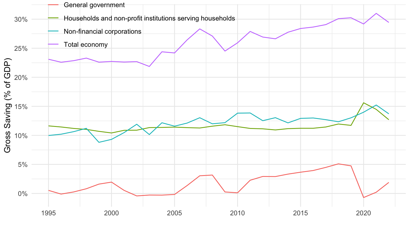
France
Code
SNA_TABLE14A %>%
  # NFK1R: Consumption of fixed capital
  # NFP5P: Gross capital formation
  filter(TRANSACT %in% c("NFB8GP"),
         SECTOR %in% c("S1", "S11", "S13", "S14_S15"),
         LOCATION %in% c("FRA")) %>%
  left_join(SNA_TABLE1 %>%
              filter(TRANSACT == "B1_GE",
                     MEASURE == "C") %>%
              select(obsTime, LOCATION, B1_GE = obsValue),
            by = c("LOCATION", "obsTime")) %>%
  left_join(SNA_TABLE14A_var$SECTOR, by = "SECTOR") %>%
  mutate(obsValue = obsValue / B1_GE) %>%
  year_to_date %>%
  select(date, obsValue, Sector) %>%
  na.omit %>%
  ggplot() + geom_line(aes(x = date, y = obsValue, color = Sector)) +
  theme_minimal() + ylab("Gross Saving (% of GDP)") + xlab("") +
  scale_x_date(breaks = seq(1920, 2100, 5) %>% paste0("-01-01") %>% as.Date,
               labels = date_format("%Y")) +

  theme(legend.position = c(0.3, 0.9),
        legend.title = element_blank()) +
  scale_y_continuous(breaks = 0.01*seq(-60, 60, 5),
labels = scales::percent_format(accuracy = 1)) 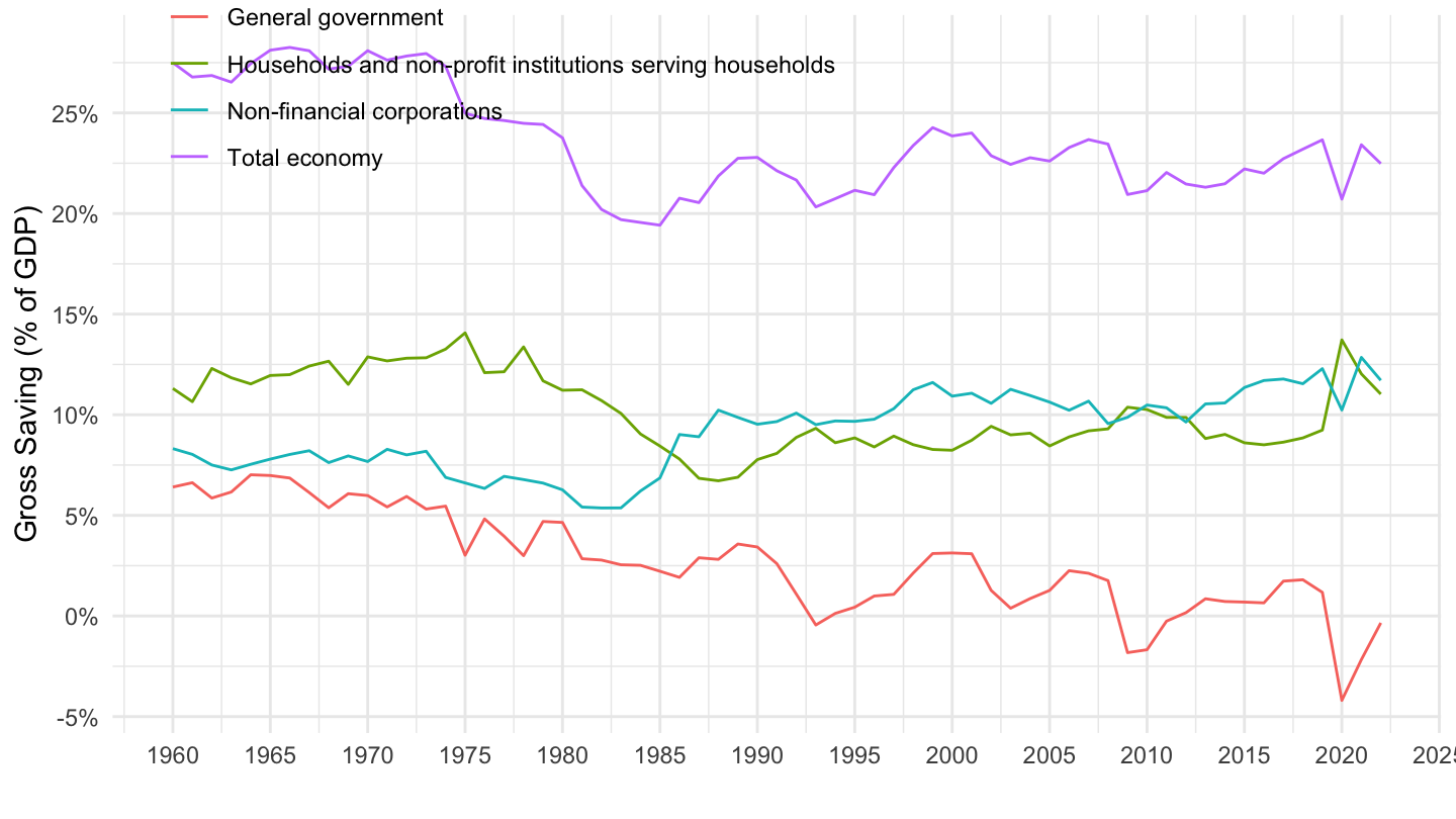
Gross capital formation (% of GDP)
Germany
Code
SNA_TABLE14A %>%
  # NFK1R: Consumption of fixed capital
  # NFP5P: Gross capital formation
  filter(TRANSACT %in% c("NFP5P"),
         SECTOR %in% c("S1", "S11", "S13", "S14_S15"),
         LOCATION %in% c("DEU")) %>%
  left_join(SNA_TABLE1 %>%
              filter(TRANSACT == "B1_GE",
                     MEASURE == "C") %>%
              select(obsTime, LOCATION, B1_GE = obsValue),
            by = c("LOCATION", "obsTime")) %>%
  left_join(SNA_TABLE14A_var$SECTOR, by = "SECTOR") %>%
  mutate(obsValue = obsValue / B1_GE) %>%
  year_to_date %>%
  ggplot() + geom_line(aes(x = date, y = obsValue, color = Sector)) +
  theme_minimal() + ylab("Gross Capital Formation (% of GDP)") + xlab("") +
  scale_x_date(breaks = seq(1920, 2100, 5) %>% paste0("-01-01") %>% as.Date,
               labels = date_format("%Y")) +

  theme(legend.position = c(0.45, 0.9),
        legend.title = element_blank()) +
  scale_y_continuous(breaks = 0.01*seq(-60, 60, 5),
                     labels = scales::percent_format(accuracy = 1),
limits = c(0, 0.35)) 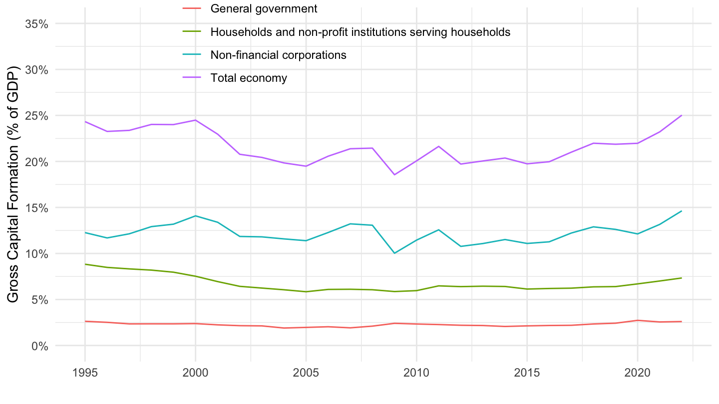
France
Code
SNA_TABLE14A %>%
  # NFK1R: Consumption of fixed capital
  # NFP5P: Gross capital formation
  filter(TRANSACT %in% c("NFP5P"),
         SECTOR %in% c("S1", "S11", "S13", "S14_S15"),
         LOCATION %in% c("FRA")) %>%
  left_join(SNA_TABLE1 %>%
              filter(TRANSACT == "B1_GE",
                     MEASURE == "C") %>%
              select(obsTime, LOCATION, B1_GE = obsValue),
            by = c("LOCATION", "obsTime")) %>%
  left_join(SNA_TABLE14A_var$SECTOR, by = "SECTOR") %>%
  mutate(obsValue = obsValue / B1_GE) %>%
  year_to_date %>%
  select(date, obsValue, Sector) %>%
  na.omit %>%
  ggplot() + geom_line(aes(x = date, y = obsValue, color = Sector)) +
  theme_minimal() + ylab("Gross Capital Formation (% of GDP)") + xlab("") +
  scale_x_date(breaks = seq(1920, 2100, 5) %>% paste0("-01-01") %>% as.Date,
               labels = date_format("%Y")) +

  theme(legend.position = c(0.65, 0.9),
        legend.title = element_blank()) +
  scale_y_continuous(breaks = 0.01*seq(-60, 60, 5),
                     labels = scales::percent_format(accuracy = 1),
limits = c(0, 0.35)) 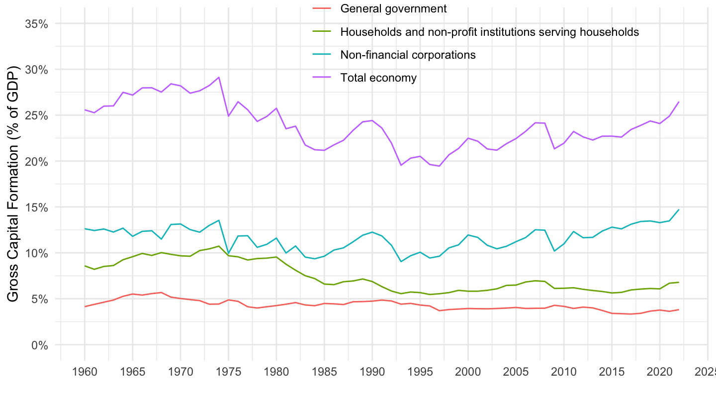
Italy
Code
SNA_TABLE14A %>%
  # NFK1R: Consumption of fixed capital
  # NFP5P: Gross capital formation
  filter(TRANSACT %in% c("NFP5P"),
         SECTOR %in% c("S1", "S11", "S13", "S14_S15"),
         LOCATION %in% c("ITA")) %>%
  left_join(SNA_TABLE1 %>%
              filter(TRANSACT == "B1_GE",
                     MEASURE == "C") %>%
              select(obsTime, LOCATION, B1_GE = obsValue),
            by = c("LOCATION", "obsTime")) %>%
  left_join(SNA_TABLE14A_var$SECTOR, by = "SECTOR") %>%
  mutate(obsValue = obsValue / B1_GE) %>%
  year_to_date %>%
  select(date, obsValue, Sector) %>%
  na.omit %>%
  ggplot() + geom_line(aes(x = date, y = obsValue, color = Sector)) +
  theme_minimal() + ylab("Gross Capital Formation (% of GDP)") + xlab("") +
  scale_x_date(breaks = seq(1920, 2100, 5) %>% paste0("-01-01") %>% as.Date,
               labels = date_format("%Y")) +

  theme(legend.position = c(0.65, 0.9),
        legend.title = element_blank()) +
  scale_y_continuous(breaks = 0.01*seq(-60, 60, 5),
                     labels = scales::percent_format(accuracy = 1),
limits = c(0, 0.35)) 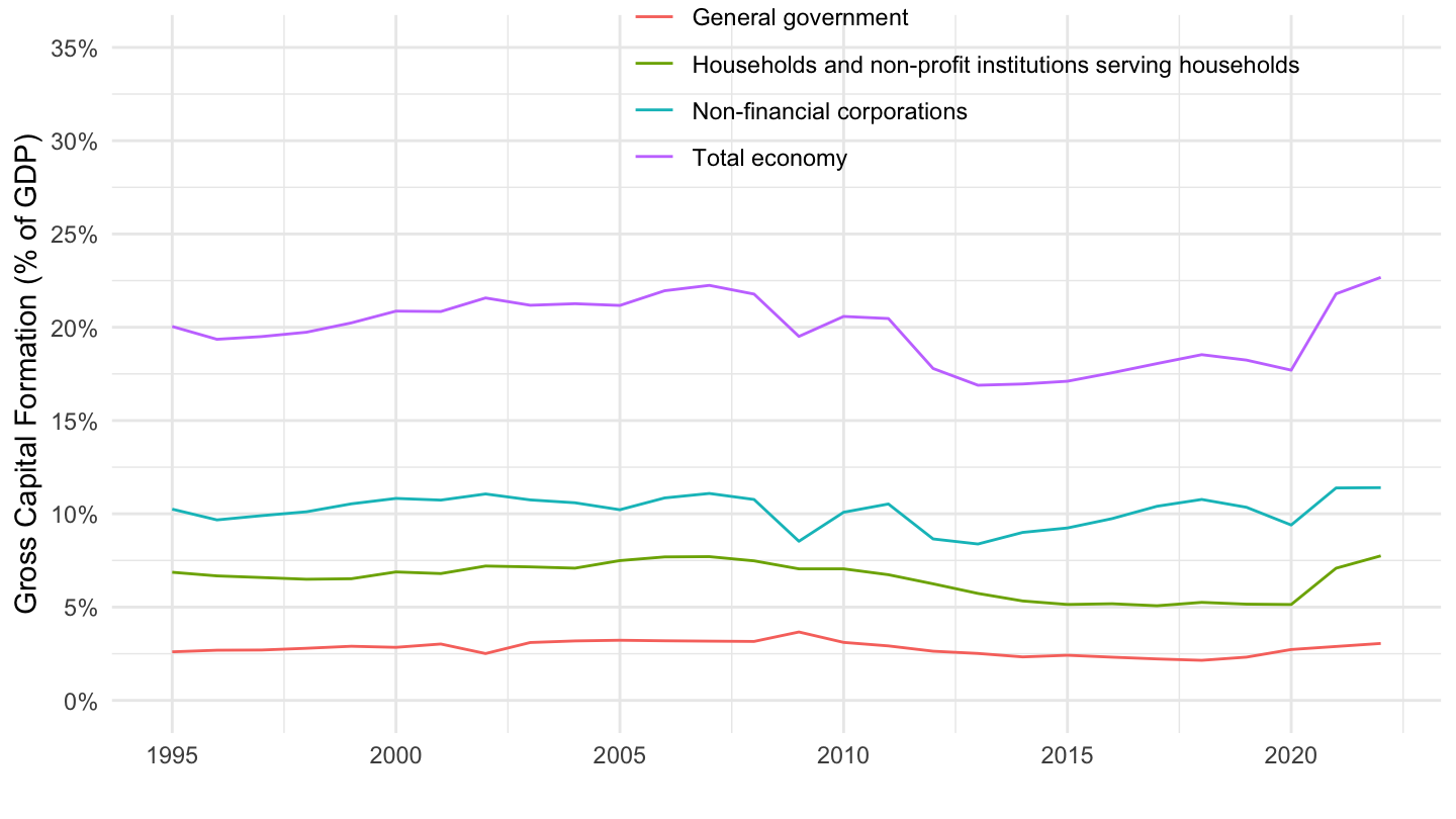
Number of observations
Gross capital formation (% of GDP)
Code
SNA_TABLE14A %>%
  # NFK1R: Consumption of fixed capital
  filter(TRANSACT %in% c("NFP5P", "B1_GE"),
         SECTOR == "S1") %>%
  left_join(SNA_TABLE14A_var$LOCATION, by = "LOCATION") %>%
  select_if(~ n_distinct(.) > 1) %>%
  select(LOCATION, Location, TRANSACT, obsTime, obsValue) %>%
  spread(TRANSACT, obsValue) %>%
  na.omit %>%
  mutate(NFP5P_B1_GE = (100*NFP5P / B1_GE)  %>% round(1) %>% paste("%")) %>%
  select(Location, obsTime, NFP5P_B1_GE) %>%
  group_by(Location) %>%
  summarise(year_first = first(obsTime),
            value_first = first(NFP5P_B1_GE),
            year_last = last(obsTime),
            value_last = last(NFP5P_B1_GE)) %>%
  {if (is_html_output()) datatable(., filter = 'top', rownames = F) else .}
Consumption of fixed capital (% of GDP)
Code
SNA_TABLE14A %>%
  # NFK1R: Consumption of fixed capital
  filter(TRANSACT %in% c("NFK1R", "B1_GE"),
         SECTOR == "S1") %>%
  left_join(SNA_TABLE14A_var$LOCATION, by = "LOCATION") %>%
  select(Location, TRANSACT, obsTime, obsValue) %>%
  spread(TRANSACT, obsValue) %>%
  na.omit %>%
  mutate(NFK1R_B1_GE = (100*NFK1R / B1_GE)  %>% round(1) %>% paste("%")) %>%
  select(Location, obsTime, NFK1R_B1_GE) %>%
  group_by(Location) %>%
  summarise(year_first = first(obsTime),
            value_first = first(NFK1R_B1_GE),
            year_last = last(obsTime),
            value_last = last(NFK1R_B1_GE)) %>%
  {if (is_html_output()) datatable(., filter = 'top', rownames = F) else .}
Net capital formation (% of GDP)
Code
SNA_TABLE14A %>%
  # NFK1R: Consumption of fixed capital
  filter(TRANSACT %in% c("NFK1R", "NFP5P", "B1_GE"),
         SECTOR == "S1") %>%
  left_join(SNA_TABLE14A_var$LOCATION, by = "LOCATION") %>%
  select(Location, TRANSACT, obsTime, obsValue) %>%
  spread(TRANSACT, obsValue) %>%
  na.omit %>%
  mutate(net_inv_B1_GE = (100*(NFP5P - NFK1R) / B1_GE)  %>% round(1) %>% paste("%")) %>%
  select(Location, obsTime, net_inv_B1_GE) %>%
  group_by(Location) %>%
  summarise(year_first = first(obsTime),
            value_first = first(net_inv_B1_GE),
            year_last = last(obsTime),
            value_last = last(net_inv_B1_GE)) %>%
  {if (is_html_output()) datatable(., filter = 'top', rownames = F) else .}
Adjustment for the change in net equity of households in pension funds (% of GDP)
Code
SNA_TABLE14A %>%
  # NFD8P: Adjustment for the change in net equity of households in pension funds
  filter(TRANSACT %in% c("NFD8P", "B1_GE"),
         SECTOR == "S1") %>%
  left_join(SNA_TABLE14A_var$LOCATION, by = "LOCATION") %>%
  select(Location, TRANSACT, obsTime, obsValue) %>%
  spread(TRANSACT, obsValue) %>%
  na.omit %>%
  mutate(NFD8P_B1_GE = (100*NFD8P / B1_GE)  %>% round(2) %>% paste("%")) %>%
  select(Location, obsTime, NFD8P_B1_GE) %>%
  group_by(Location) %>%
  summarise(year_first = first(obsTime),
            value_first = first(NFD8P_B1_GE),
            year_last = last(obsTime),
            value_last = last(NFD8P_B1_GE)) %>%
  {if (is_html_output()) datatable(., filter = 'top', rownames = F) else .}
Time Series
Gross capital formation (% of GDP)
All
S1
Code
SNA_TABLE14A %>%
  # NFK1R: Consumption of fixed capital
  # NFP5P: Gross capital formation
  filter(TRANSACT %in% c("NFK1R", "NFP5P", "B1_GE"),
         SECTOR == "S1",
         LOCATION %in% c("FRA", "USA", "DEU", "JPN")) %>%
  left_join(SNA_TABLE14A_var$LOCATION, by = "LOCATION") %>%
  select(Location, TRANSACT, obsTime, obsValue) %>%
  spread(TRANSACT, obsValue) %>%
  na.omit %>%
  year_to_date %>%
  mutate(obsValue = (NFP5P) / B1_GE) %>%
  left_join(colors, by = c("Location" = "country")) %>%
  ggplot() + geom_line(aes(x = date, y = obsValue, color = color)) +
  scale_color_identity() + theme_minimal() + add_4flags +
  scale_x_date(breaks = seq(1920, 2100, 5) %>% paste0("-01-01") %>% as.Date,
               labels = date_format("%Y")) +
  scale_y_continuous(breaks = 0.01*seq(-60, 60, 1),
                     labels = scales::percent_format(accuracy = 1)) +
  ylab("Gross Capital Formation (% of GDP)") + xlab("")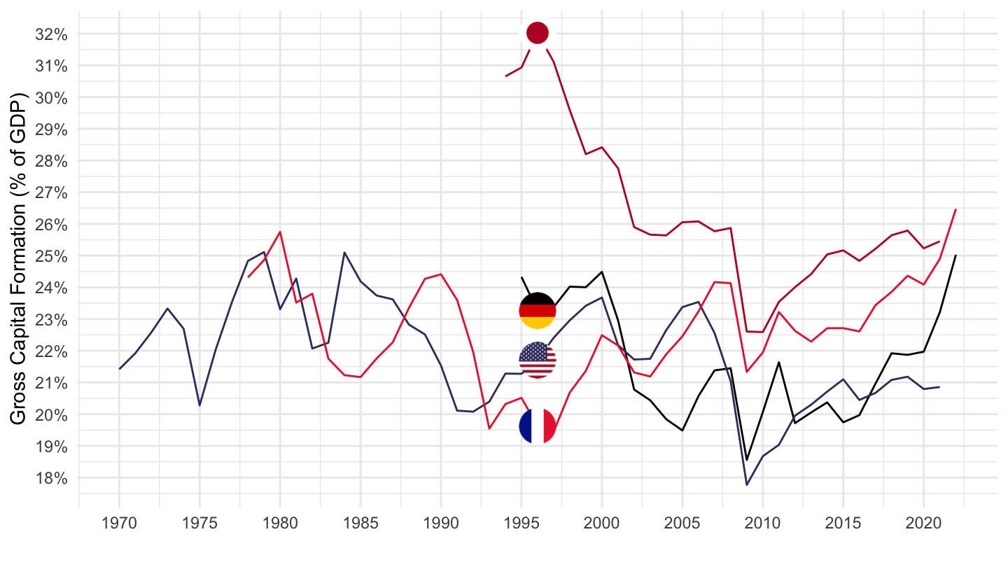
S11
Code
SNA_TABLE14A %>%
  # NFK1R: Consumption of fixed capital
  # NFP5P: Gross capital formation
  filter(TRANSACT %in% c("NFP5P"),
         SECTOR == "S11",
         LOCATION %in% c("FRA", "USA", "DEU", "JPN")) %>%
  left_join(SNA_TABLE14A_var$LOCATION, by = "LOCATION") %>%
  left_join(SNA_TABLE1 %>%
              filter(TRANSACT == "B1_GE",
                     MEASURE == "C") %>%
              select(obsTime, LOCATION, B1_GE = obsValue),
            by = c("LOCATION", "obsTime")) %>%
  mutate(obsValue = obsValue / B1_GE) %>%
  year_to_date %>%
  left_join(colors, by = c("Location" = "country")) %>%
  ggplot() + geom_line(aes(x = date, y = obsValue, color = color)) +
  scale_color_identity() + theme_minimal() + add_4flags +
  scale_x_date(breaks = seq(1920, 2100, 5) %>% paste0("-01-01") %>% as.Date,
               labels = date_format("%Y")) +
  scale_y_continuous(breaks = 0.01*seq(-60, 60, 1),
                     labels = scales::percent_format(accuracy = 1)) +
  ylab("Gross Capital Formation (% of GDP)") + xlab("")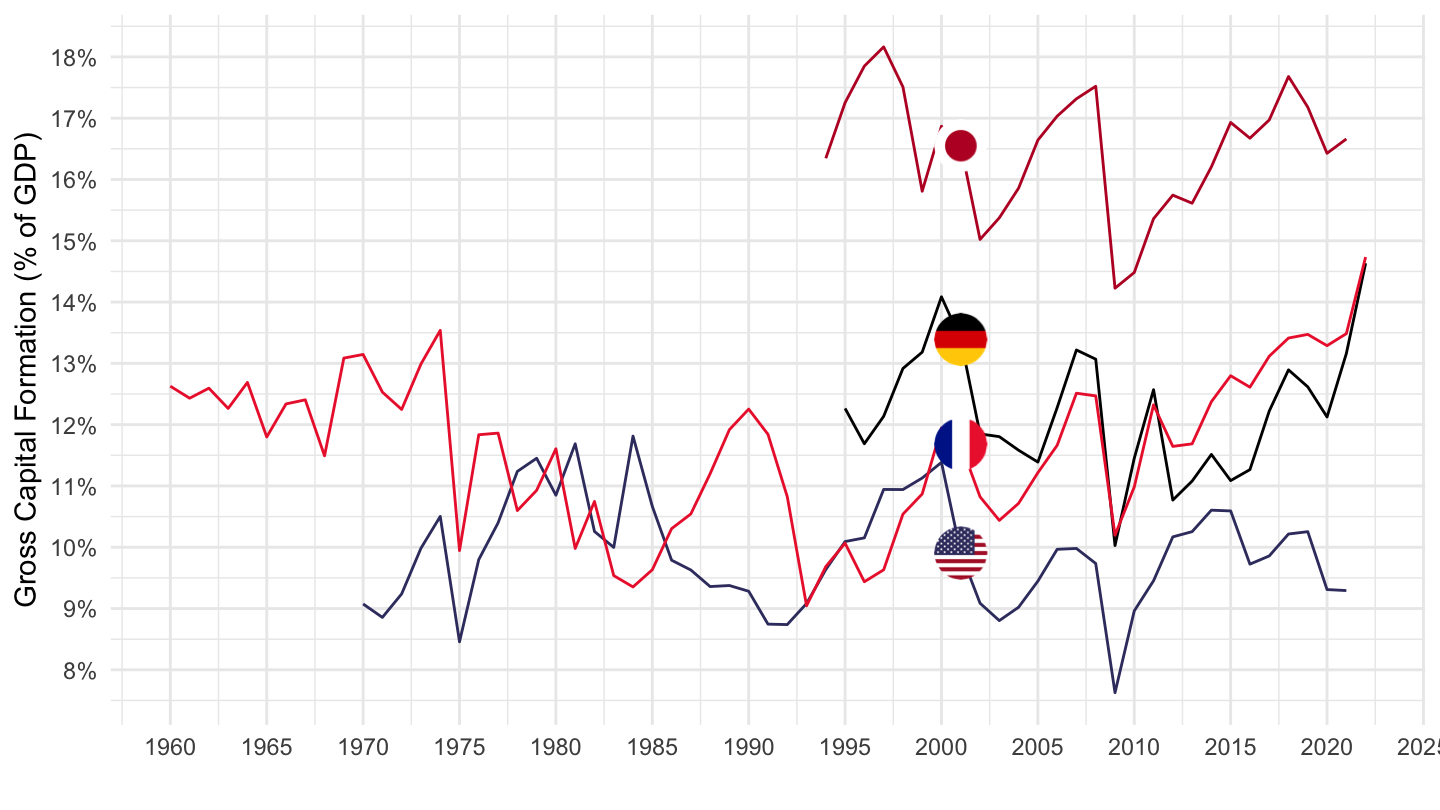
S13
5
Code
SNA_TABLE14A %>%
  # NFK1R: Consumption of fixed capital
  # NFP5P: Gross capital formation
  filter(TRANSACT %in% c("NFP5P"),
         SECTOR == "S13",
         LOCATION %in% c("FRA", "USA", "DEU", "JPN")) %>%
  left_join(SNA_TABLE14A_var$LOCATION, by = "LOCATION") %>%
  left_join(SNA_TABLE1 %>%
              filter(TRANSACT == "B1_GE",
                     MEASURE == "C") %>%
              select(obsTime, LOCATION, B1_GE = obsValue),
            by = c("LOCATION", "obsTime")) %>%
  mutate(obsValue = obsValue / B1_GE) %>%
  year_to_date %>%
  left_join(colors, by = c("Location" = "country")) %>%
  ggplot() + geom_line(aes(x = date, y = obsValue, color = color)) +
  scale_color_identity() + theme_minimal() + add_4flags +
  scale_x_date(breaks = seq(1920, 2100, 5) %>% paste0("-01-01") %>% as.Date,
               labels = date_format("%Y")) +
  scale_y_continuous(breaks = 0.01*seq(-60, 60, 1),
                     labels = scales::percent_format(accuracy = 1)) +
  ylab("Gross Capital Formation (% of GDP) - Government") + xlab("")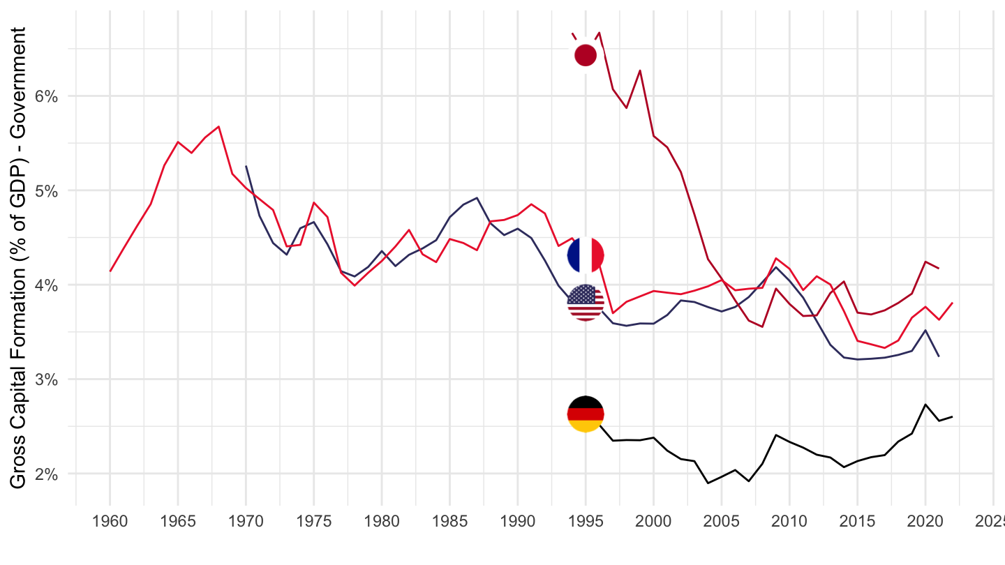
France, Unnited STates, Germany
Code
SNA_TABLE14A %>%
  # NFK1R: Consumption of fixed capital
  # NFP5P: Gross capital formation
  filter(TRANSACT %in% c("NFP5P"),
         SECTOR %in% c("S13"),
         LOCATION %in% c("FRA", "USA", "DEU")) %>%
  left_join(SNA_TABLE14A_var$LOCATION, by = "LOCATION") %>%
  left_join(SNA_TABLE1 %>%
              filter(TRANSACT == "B1_GE",
                     MEASURE == "C") %>%
              select(obsTime, LOCATION, B1_GE = obsValue),
            by = c("LOCATION", "obsTime")) %>%
  mutate(obsValue = obsValue / B1_GE) %>%
  year_to_date %>%
  filter(date >= as.Date("1995-01-01")) %>%
  left_join(colors, by = c("Location" = "country")) %>%
  mutate(color = ifelse(LOCATION == "USA", color2, color)) %>%
  ggplot() + geom_line(aes(x = date, y = obsValue, color = color)) +
  scale_color_identity() + theme_minimal() + add_3flags +
  scale_x_date(breaks = seq(1920, 2100, 2) %>% paste0("-01-01") %>% as.Date,
               labels = date_format("%Y")) +
  scale_y_continuous(breaks = 0.01*seq(-60, 60, 0.5),
                     labels = scales::percent_format(accuracy = .1)) +
  ylab("Gross Capital Formation (% of GDP) - Government") + xlab("")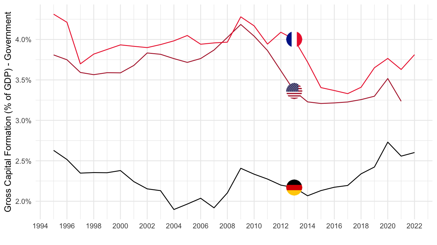
More countries
Code
SNA_TABLE14A %>%
  # NFK1R: Consumption of fixed capital
  # NFP5P: Gross capital formation
  filter(TRANSACT %in% c("NFP5P"),
         SECTOR %in% c("S13"),
         LOCATION %in% c("PRT", "USA", "DEU", "ITA", "ESP", "GRC")) %>%
  left_join(SNA_TABLE14A_var$LOCATION, by = "LOCATION") %>%
  left_join(SNA_TABLE1 %>%
              filter(TRANSACT == "B1_GE",
                     MEASURE == "C") %>%
              select(obsTime, LOCATION, B1_GE = obsValue),
            by = c("LOCATION", "obsTime")) %>%
  mutate(obsValue = obsValue / B1_GE) %>%
  year_to_date %>%
  filter(date >= as.Date("1995-01-01")) %>%
  left_join(colors, by = c("Location" = "country")) %>%
  mutate(color = ifelse(LOCATION == "USA", color2, color)) %>%
  ggplot() + geom_line(aes(x = date, y = obsValue, color = color)) +
  scale_color_identity() + theme_minimal() + add_6flags +
  scale_x_date(breaks = seq(1920, 2100, 2) %>% paste0("-01-01") %>% as.Date,
               labels = date_format("%Y")) +
  scale_y_continuous(breaks = 0.01*seq(-60, 60, 0.5),
                     labels = scales::percent_format(accuracy = .1)) +
  ylab("Gross Capital Formation (% of GDP) - Government") + xlab("")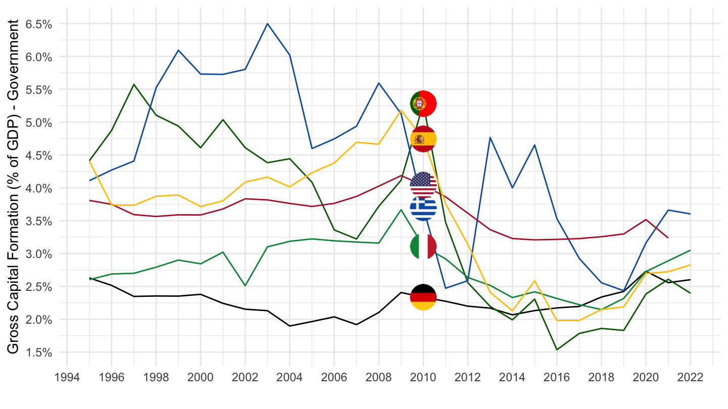
Code
SNA_TABLE14A %>%
  # NFK1R: Consumption of fixed capital
  # NFP5P: Gross capital formation
  filter(TRANSACT %in% c("NFP5P"),
         SECTOR %in% c("S13"),
         LOCATION %in% c("PRT", "USA", "DEU", "ITA", "ESP", "GRC")) %>%
  left_join(SNA_TABLE14A_var$LOCATION, by = "LOCATION") %>%
  left_join(SNA_TABLE1 %>%
              filter(TRANSACT == "B1_GE",
                     MEASURE == "C") %>%
              select(obsTime, LOCATION, B1_GE = obsValue),
            by = c("LOCATION", "obsTime")) %>%
  mutate(obsValue = obsValue / B1_GE) %>%
  year_to_date %>%
  filter(date >= as.Date("2012-01-01")) %>%
  left_join(colors, by = c("Location" = "country")) %>%
  mutate(color = ifelse(LOCATION == "USA", color2, color)) %>%
  ggplot() + geom_line(aes(x = date, y = obsValue, color = color)) +
  scale_color_identity() + theme_minimal() + add_6flags +
  scale_x_date(breaks = seq(1920, 2100, 1) %>% paste0("-01-01") %>% as.Date,
               labels = date_format("%Y")) +
  scale_y_continuous(breaks = 0.01*seq(-60, 60, 0.5),
                     labels = scales::percent_format(accuracy = .1)) +
  ylab("Gross Capital Formation (% of GDP) - Government") + xlab("")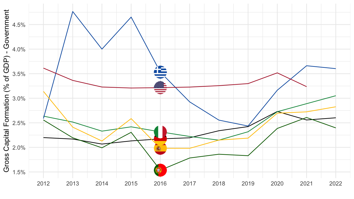
1994-
Code
SNA_TABLE14A %>%
  # NFK1R: Consumption of fixed capital
  # NFP5P: Gross capital formation
  filter(TRANSACT %in% c("NFK1R", "NFP5P", "B1_GE"),
         SECTOR == "S1",
         LOCATION %in% c("FRA", "USA", "DEU", "JPN")) %>%
  left_join(SNA_TABLE14A_var$LOCATION, by = "LOCATION") %>%
  select(Location, TRANSACT, obsTime, obsValue) %>%
  spread(TRANSACT, obsValue) %>%
  na.omit %>%
  year_to_date %>%
  filter(date >= as.Date("1994-01-01")) %>%
  mutate(obsValue = (NFP5P) / B1_GE) %>%
  left_join(colors, by = c("Location" = "country")) %>%
  ggplot() + geom_line(aes(x = date, y = obsValue, color = color)) +
  scale_color_identity() + theme_minimal() + add_4flags +
  scale_x_date(breaks = seq(1920, 2100, 5) %>% paste0("-01-01") %>% as.Date,
               labels = date_format("%Y")) +
  scale_y_continuous(breaks = 0.01*seq(-60, 60, 1),
                     labels = scales::percent_format(accuracy = 1)) +
  ylab("Gross Capital Formation (% of GDP)") + xlab("")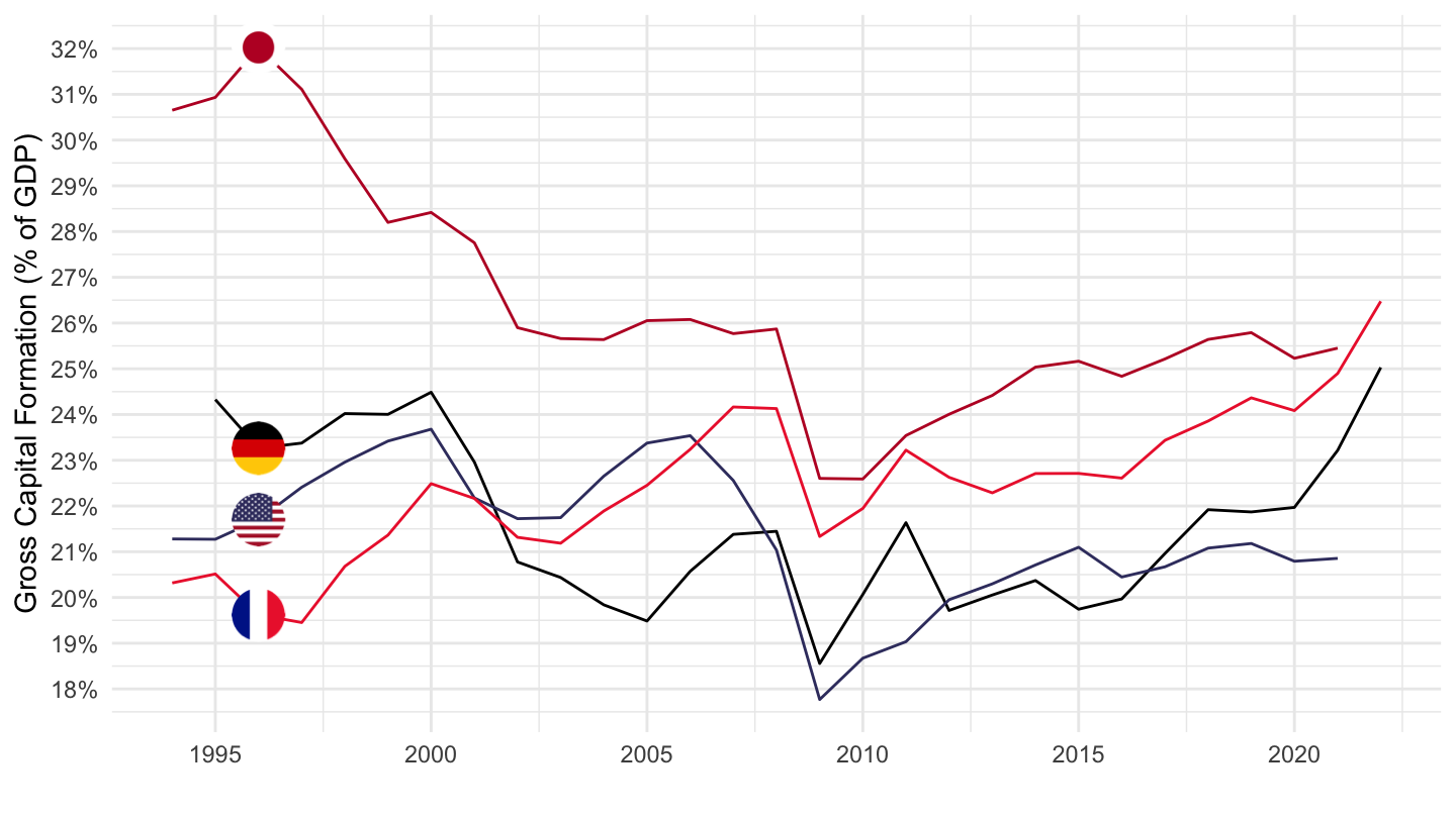
France
Disposable Income, GDP
All
Code
SNA_TABLE14A %>%
  filter((SECTOR %in% c("S14_S15", "S1") & TRANSACT == "NFB6GP") |
           (SECTOR == "S1" & TRANSACT == "B1_GE"),
         LOCATION %in% c("FRA")) %>%
  year_to_date %>%
  left_join(SNA_TABLE14A_var$TRANSACT, by = "TRANSACT") %>%
  left_join(SNA_TABLE14A_var$SECTOR, by = "SECTOR") %>%
  group_by(TRANSACT, SECTOR) %>%
  arrange(date) %>%
  mutate(obsValue = 100*obsValue/obsValue[1]) %>%
  ggplot() + geom_line(aes(x = date, y = obsValue, color = paste0(Transact, " - ", Sector))) + theme_minimal() +
  scale_color_manual(values = viridis(4)[1:3]) +
  theme(legend.position = c(0.4, 0.9),
        legend.title = element_blank()) +
  scale_x_date(breaks = seq(1920, 2100, 5) %>% paste0("-01-01") %>% as.Date,
               labels = date_format("%Y")) +
  scale_y_log10(breaks = seq(1000, 50000, 1000)) +
  ylab("Indice 1995 = 100") + xlab("")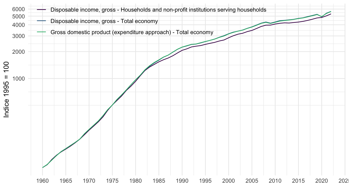
1990-
Code
SNA_TABLE14A %>%
  filter((SECTOR %in% c("S14_S15", "S1") & TRANSACT == "NFB6GP") |
           (SECTOR == "S1" & TRANSACT == "B1_GE"),
         LOCATION %in% c("FRA")) %>%
  year_to_date %>%
  filter(date >= as.Date("1990-01-01")) %>%
  left_join(SNA_TABLE14A_var$TRANSACT, by = "TRANSACT") %>%
  left_join(SNA_TABLE14A_var$SECTOR, by = "SECTOR") %>%
  group_by(TRANSACT, SECTOR) %>%
  mutate(obsValue = 100*obsValue/obsValue[1]) %>%
  mutate(Variable = paste0(Transact, " - ", Sector)) %>%
  ggplot() + geom_line(aes(x = date, y = obsValue, color = Variable)) +
  theme_minimal() + ylab("Indice 1990 = 100") + xlab("") +
  scale_color_manual(values = viridis(4)[1:3]) +
  theme(legend.position = c(0.45, 0.9),
        legend.title = element_blank()) +
  scale_x_date(breaks = seq(1920, 2100, 5) %>% paste0("-01-01") %>% as.Date,
               labels = date_format("%Y")) +
  scale_y_log10(breaks = seq(100, 300, 10))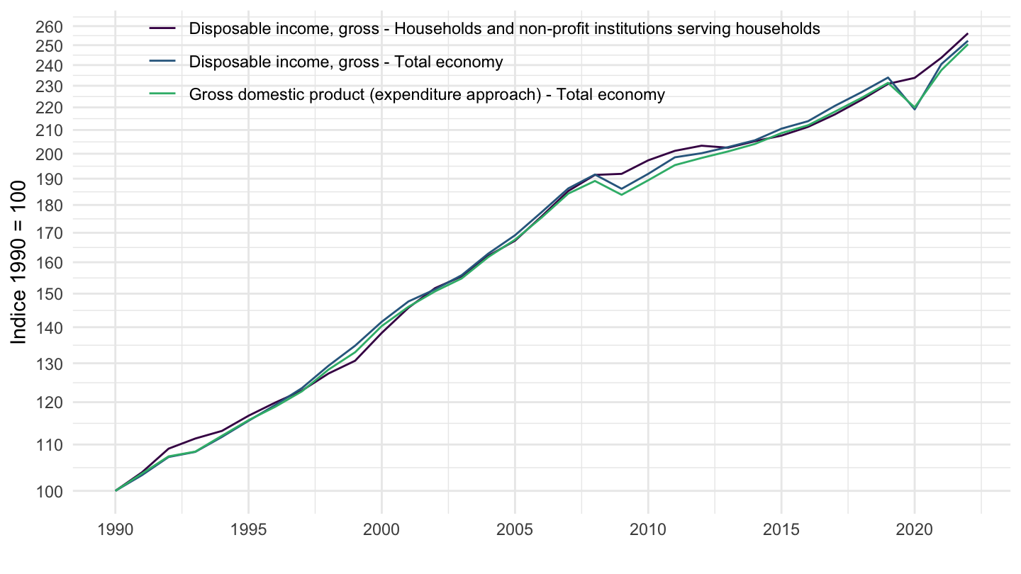
1995-
Code
SNA_TABLE14A %>%
  filter((SECTOR %in% c("S14_S15", "S1") & TRANSACT == "NFB6GP") |
           (SECTOR == "S1" & TRANSACT == "B1_GE"),
         LOCATION %in% c("FRA")) %>%
  year_to_date %>%
  filter(date >= as.Date("1995-01-01")) %>%
  left_join(SNA_TABLE14A_var$TRANSACT, by = "TRANSACT") %>%
  left_join(SNA_TABLE14A_var$SECTOR, by = "SECTOR") %>%
  group_by(TRANSACT, SECTOR) %>%
  mutate(obsValue = 100*obsValue/obsValue[1]) %>%
  mutate(Variable = paste0(Transact, " - ", Sector)) %>%
  ggplot() + geom_line(aes(x = date, y = obsValue, color = Variable)) +
  theme_minimal() + ylab("Indice 1995 = 100") + xlab("") +
  scale_color_manual(values = viridis(4)[1:3]) +
  theme(legend.position = c(0.45, 0.9),
        legend.title = element_blank()) +
  scale_x_date(breaks = seq(1920, 2100, 5) %>% paste0("-01-01") %>% as.Date,
               labels = date_format("%Y")) +
  scale_y_log10(breaks = seq(100, 300, 5))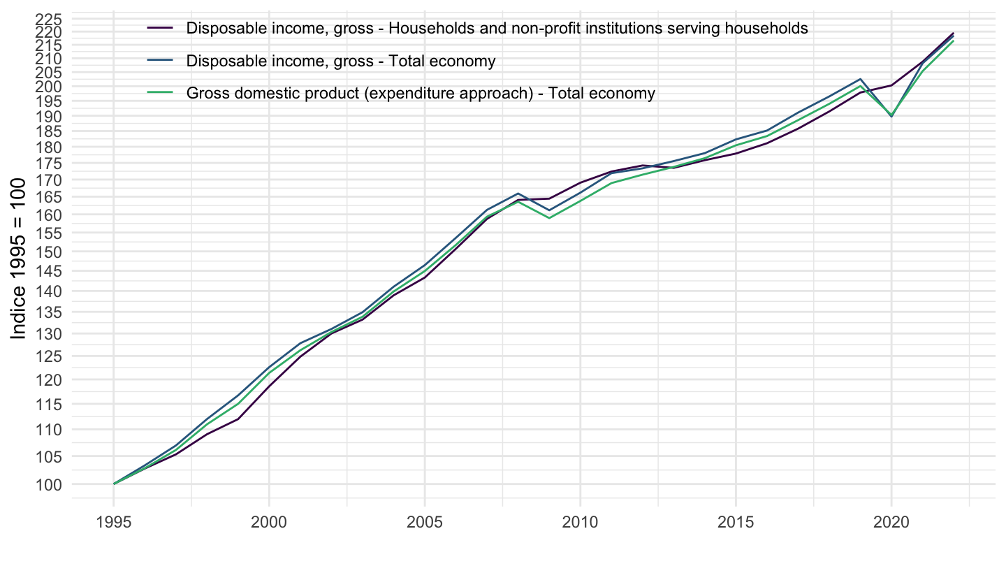
1996-
Code
SNA_TABLE14A %>%
  filter((SECTOR %in% c("S14_S15", "S1") & TRANSACT == "NFB6GP") |
           (SECTOR == "S1" & TRANSACT == "B1_GE"),
         LOCATION %in% c("FRA")) %>%
  year_to_date %>%
  filter(date >= as.Date("1996-01-01")) %>%
  left_join(SNA_TABLE14A_var$TRANSACT, by = "TRANSACT") %>%
  left_join(SNA_TABLE14A_var$SECTOR, by = "SECTOR") %>%
  group_by(TRANSACT, SECTOR) %>%
  mutate(obsValue = 100*obsValue/obsValue[1]) %>%
  mutate(Variable = paste0(Transact, " - ", Sector)) %>%
  ggplot() + geom_line(aes(x = date, y = obsValue, color = Variable)) +
  theme_minimal() + ylab("Indice 1996 = 100") + xlab("") +
  scale_color_manual(values = viridis(4)[1:3]) +
  theme(legend.position = c(0.45, 0.9),
        legend.title = element_blank()) +
  scale_x_date(breaks = seq(1920, 2100, 2) %>% paste0("-01-01") %>% as.Date,
               labels = date_format("%Y")) +
  scale_y_log10(breaks = seq(100, 300, 5))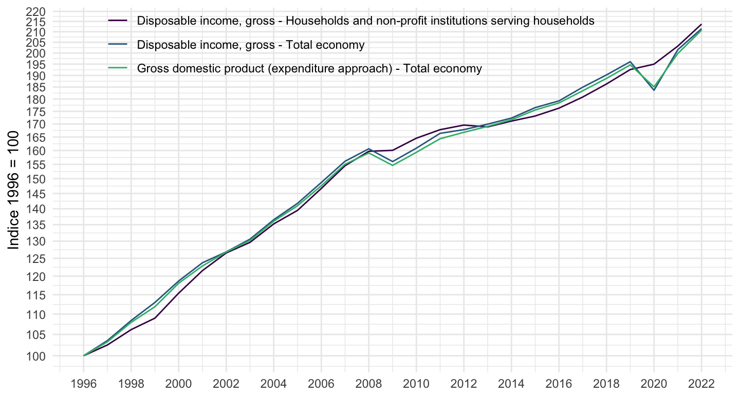
2008-
Code
SNA_TABLE14A %>%
  filter((SECTOR %in% c("S14_S15", "S1") & TRANSACT == "NFB6GP") |
           (SECTOR == "S1" & TRANSACT == "B1_GE"),
         LOCATION %in% c("FRA")) %>%
  year_to_date %>%
  filter(date >= as.Date("2008-01-01")) %>%
  left_join(SNA_TABLE14A_var$TRANSACT, by = "TRANSACT") %>%
  left_join(SNA_TABLE14A_var$SECTOR, by = "SECTOR") %>%
  group_by(TRANSACT, SECTOR) %>%
  mutate(obsValue = 100*obsValue/obsValue[1]) %>%
  mutate(Variable = paste0(Transact, " - ", Sector)) %>%
  ggplot() + geom_line(aes(x = date, y = obsValue, color = Variable)) +
  theme_minimal() + ylab("Indice 2008 = 100") + xlab("") +
  scale_color_manual(values = viridis(4)[1:3]) +
  theme(legend.position = c(0.45, 0.9),
        legend.title = element_blank()) +
  scale_x_date(breaks = seq(1920, 2100, 1) %>% paste0("-01-01") %>% as.Date,
               labels = date_format("%Y")) +
  scale_y_log10(breaks = seq(100, 300, 5))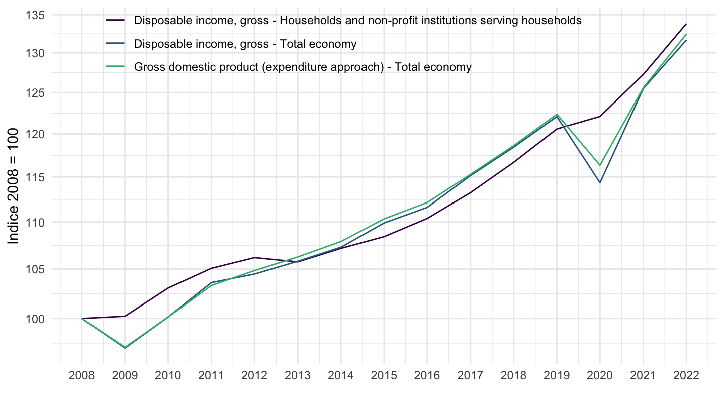
B6NS1 - Net National Disposable Income / GDP
B6GS1 - Gross National Disposable Income / GDP
Households (% of GDP)
France, Germany, Belgium, Netherlands, Italy
Code
SNA_TABLE14A %>%
  filter((SECTOR == "S14_S15" & TRANSACT == "NFB6GP") |
           (SECTOR == "S1" & TRANSACT == "B1_GE"),
         LOCATION %in% c("FRA", "DEU", "BEL", "ESP", "NLD", "ITA")) %>%
  year_to_date %>%
  left_join(SNA_TABLE14A_var$LOCATION, by = "LOCATION") %>%
  select(Location, date, TRANSACT, obsValue) %>%
  spread(TRANSACT, obsValue) %>%
  group_by(Location) %>%
  mutate(obsValue = NFB6GP / B1_GE) %>%
  select(Location, date, obsValue) %>%
  na.omit %>%
  left_join(colors, by = c("Location" = "country")) %>%
  mutate(color = ifelse(Location == "Netherlands", color2, color)) %>%
  filter(date >= as.Date("1995-01-01")) %>%
  ggplot() + geom_line(aes(x = date, y = obsValue, color = color)) +
  scale_color_identity() + theme_minimal() + add_6flags +
  scale_x_date(breaks = seq(1920, 2100, 5) %>% paste0("-01-01") %>% as.Date,
               labels = date_format("%Y")) +
  scale_y_continuous(breaks = 0.01*seq(-10, 120, 1),
                     labels = scales::percent_format(accuracy = 1)) +
  ylab("Gross National Disposable Income (% of GDP)") + xlab("")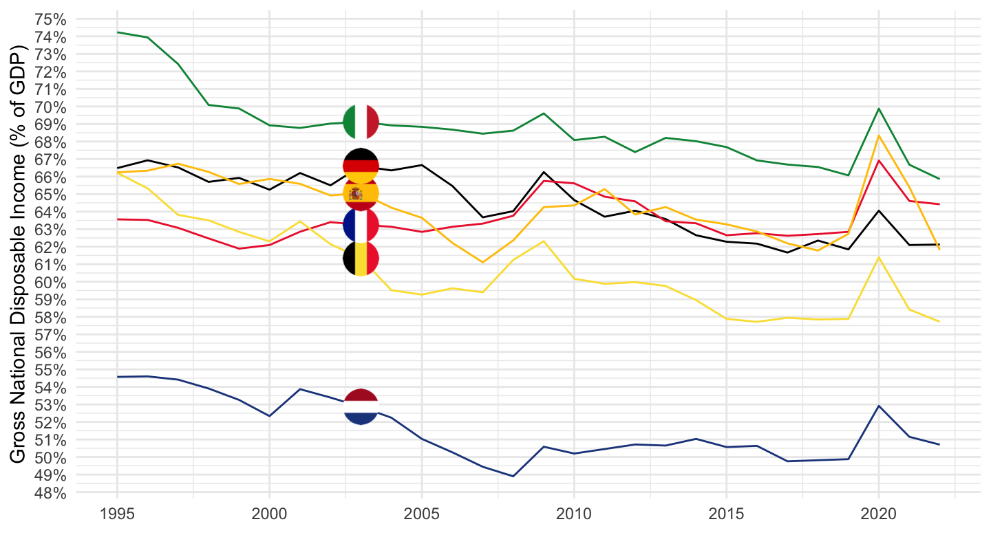
France, Germany, U.S., Denmark
Code
SNA_TABLE14A %>%
  filter((SECTOR == "S14_S15" & TRANSACT == "NFB6GP") |
           (SECTOR == "S1" & TRANSACT == "B1_GE"),
         LOCATION %in% c("FRA", "DEU", "USA", "DNK")) %>%
  year_to_date %>%
  left_join(SNA_TABLE14A_var$LOCATION, by = "LOCATION") %>%
  select(Location, date, TRANSACT, obsValue) %>%
  spread(TRANSACT, obsValue) %>%
  group_by(Location) %>%
  mutate(obsValue = NFB6GP / B1_GE) %>%
  select(Location, date, obsValue) %>%
  na.omit %>%
  left_join(colors, by = c("Location" = "country")) %>%
  mutate(color = ifelse(Location == "Netherlands", color2, color)) %>%
  filter(date >= as.Date("1995-01-01")) %>%
  ggplot() + geom_line(aes(x = date, y = obsValue, color = color)) +
  scale_color_identity() + theme_minimal() + add_4flags +
  scale_x_date(breaks = seq(1920, 2100, 5) %>% paste0("-01-01") %>% as.Date,
               labels = date_format("%Y")) +
  scale_y_continuous(breaks = 0.01*seq(-10, 120, 1),
                     labels = scales::percent_format(accuracy = 1)) +
  ylab("Gross National Disposable Income (% of GDP)") + xlab("")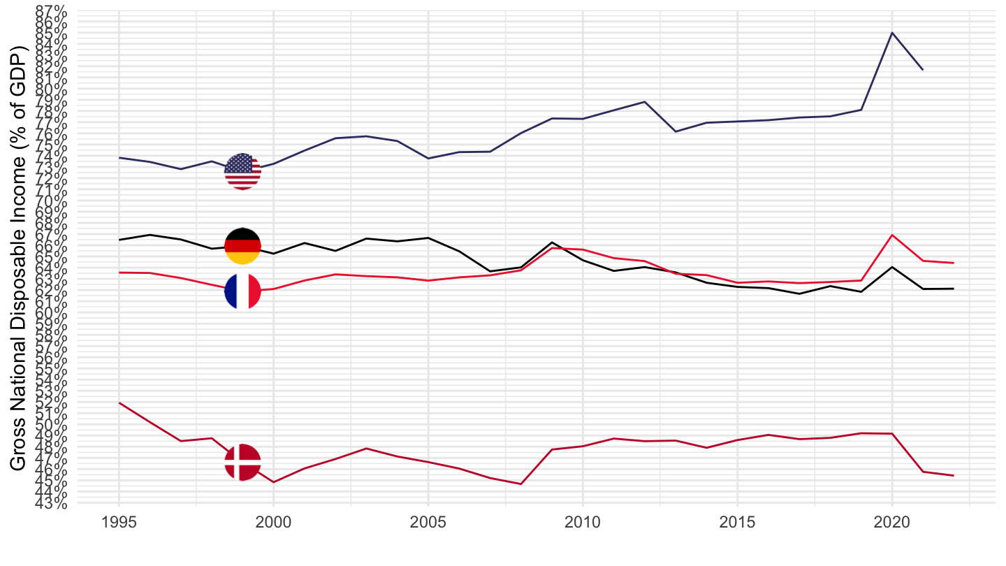
Corporations (% of GDP)
Code
SNA_TABLE14A %>%
  filter((SECTOR == "S13" & TRANSACT == "NFB6GP") |
           (SECTOR == "S1" & TRANSACT == "B1_GE"),
         LOCATION %in% c("FRA", "DEU", "BEL", "ESP", "NLD", "ITA")) %>%
  year_to_date %>%
  left_join(SNA_TABLE14A_var$LOCATION, by = "LOCATION") %>%
  select(Location, date, TRANSACT, obsValue) %>%
  spread(TRANSACT, obsValue) %>%
  group_by(Location) %>%
  mutate(obsValue = NFB6GP / B1_GE) %>%
  select(Location, date, obsValue) %>%
  na.omit %>%
  left_join(colors, by = c("Location" = "country")) %>%
  mutate(color = ifelse(Location == "Netherlands", color2, color)) %>%
  filter(date >= as.Date("1995-01-01")) %>%
  ggplot() + geom_line(aes(x = date, y = obsValue, color = color)) +
  scale_color_identity() + theme_minimal() + add_6flags +
  scale_x_date(breaks = seq(1920, 2100, 5) %>% paste0("-01-01") %>% as.Date,
               labels = date_format("%Y")) +
  scale_y_continuous(breaks = 0.01*seq(-10, 120, 1),
                     labels = scales::percent_format(accuracy = 1)) +
  ylab("Gross National Disposable Income (% of GDP)") + xlab("")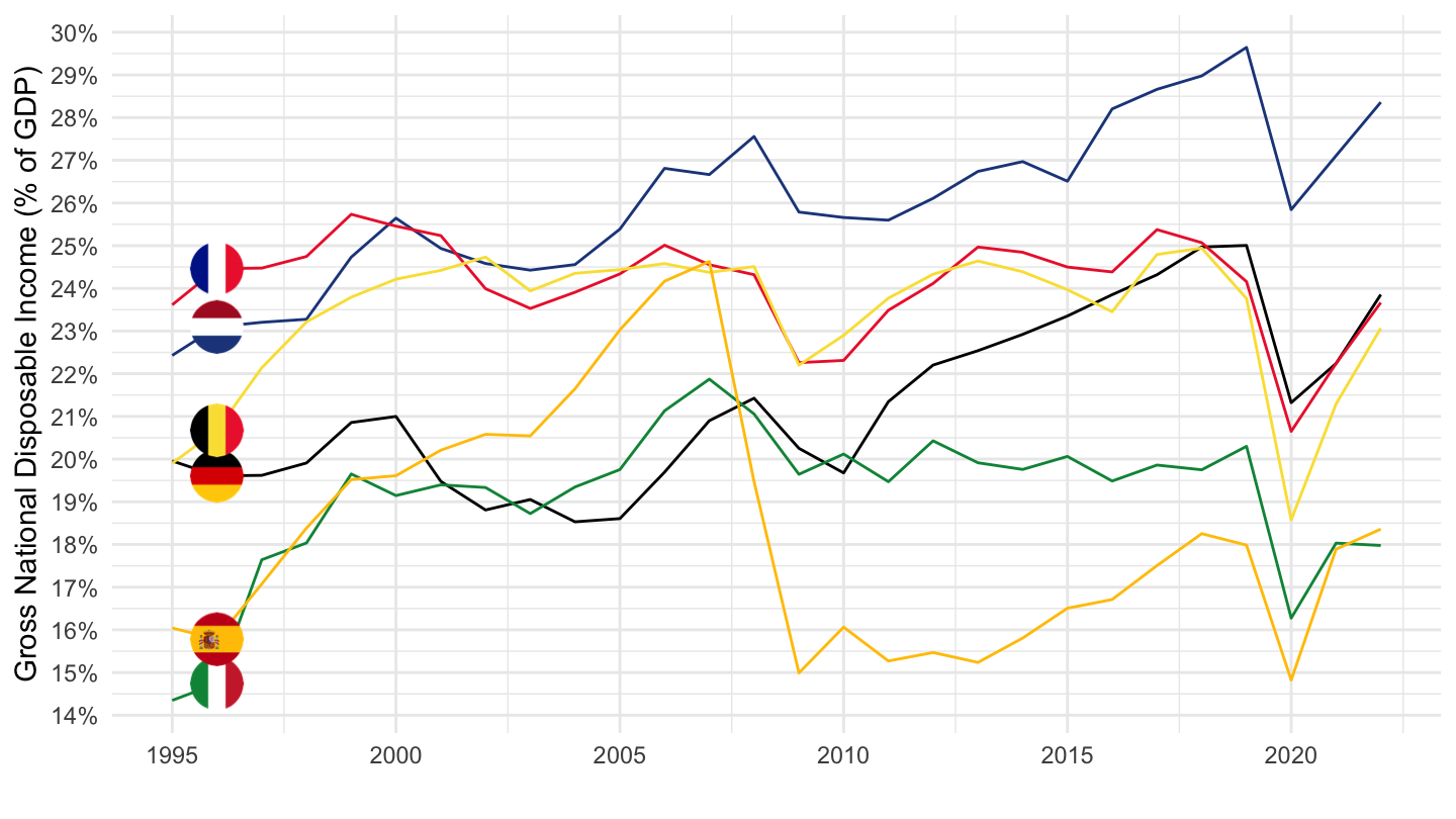
Governments (% of GDP)
Code
SNA_TABLE14A %>%
  filter((SECTOR == "S11" & TRANSACT == "NFB6GP") |
           (SECTOR == "S1" & TRANSACT == "B1_GE"),
         LOCATION %in% c("FRA", "DEU", "BEL", "ESP", "NLD", "ITA")) %>%
  year_to_date %>%
  left_join(SNA_TABLE14A_var$LOCATION, by = "LOCATION") %>%
  select(Location, date, TRANSACT, obsValue) %>%
  spread(TRANSACT, obsValue) %>%
  group_by(Location) %>%
  mutate(obsValue = NFB6GP / B1_GE) %>%
  select(Location, date, obsValue) %>%
  na.omit %>%
  left_join(colors, by = c("Location" = "country")) %>%
  mutate(color = ifelse(Location == "Netherlands", color2, color)) %>%
  filter(date >= as.Date("1995-01-01")) %>%
  ggplot() + geom_line(aes(x = date, y = obsValue, color = color)) +
  scale_color_identity() + theme_minimal() + add_6flags +
  scale_x_date(breaks = seq(1920, 2100, 5) %>% paste0("-01-01") %>% as.Date,
               labels = date_format("%Y")) +
  scale_y_continuous(breaks = 0.01*seq(-10, 120, 1),
                     labels = scales::percent_format(accuracy = 1)) +
  ylab("Gross National Disposable Income (% of GDP)") + xlab("")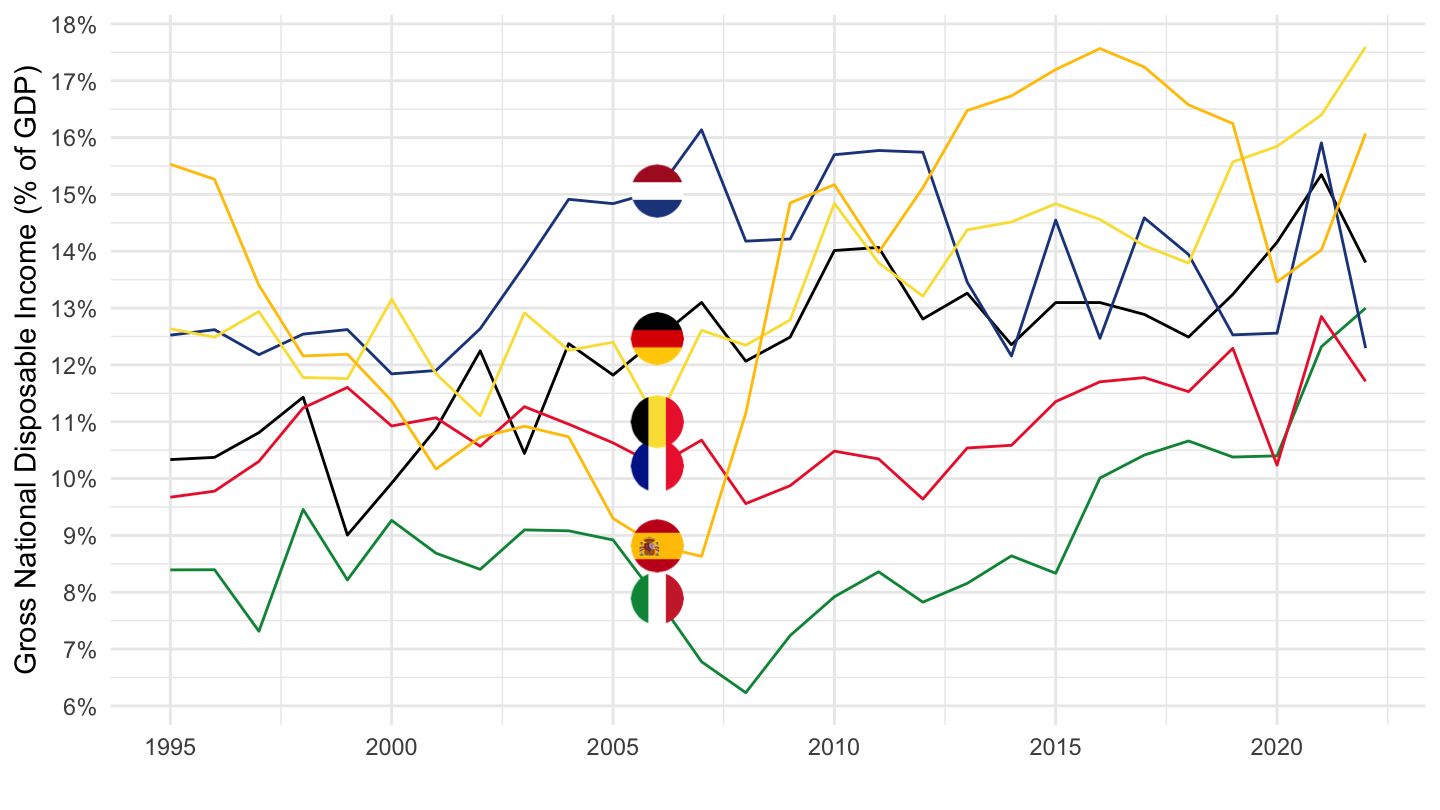
All (% of GDP)
Code
SNA_TABLE14A %>%
  filter((SECTOR == "S1" & TRANSACT == "NFB6GP") |
           (SECTOR == "S1" & TRANSACT == "B1_GE"),
         LOCATION %in% c("FRA", "DEU", "BEL", "ESP", "NLD", "ITA")) %>%
  year_to_date %>%
  left_join(SNA_TABLE14A_var$LOCATION, by = "LOCATION") %>%
  select(Location, date, TRANSACT, obsValue) %>%
  spread(TRANSACT, obsValue) %>%
  group_by(Location) %>%
  mutate(obsValue = NFB6GP / B1_GE) %>%
  select(Location, date, obsValue) %>%
  na.omit %>%
  left_join(colors, by = c("Location" = "country")) %>%
  mutate(color = ifelse(Location == "Netherlands", color2, color)) %>%
  filter(date >= as.Date("1995-01-01")) %>%
  ggplot() + geom_line(aes(x = date, y = obsValue, color = color)) +
  scale_color_identity() + theme_minimal() + add_6flags +
  scale_x_date(breaks = seq(1920, 2100, 5) %>% paste0("-01-01") %>% as.Date,
               labels = date_format("%Y")) +
  scale_y_continuous(breaks = 0.01*seq(-10, 120, 1),
                     labels = scales::percent_format(accuracy = 1)) +
  ylab("Gross National Disposable Income (% of GDP)") + xlab("")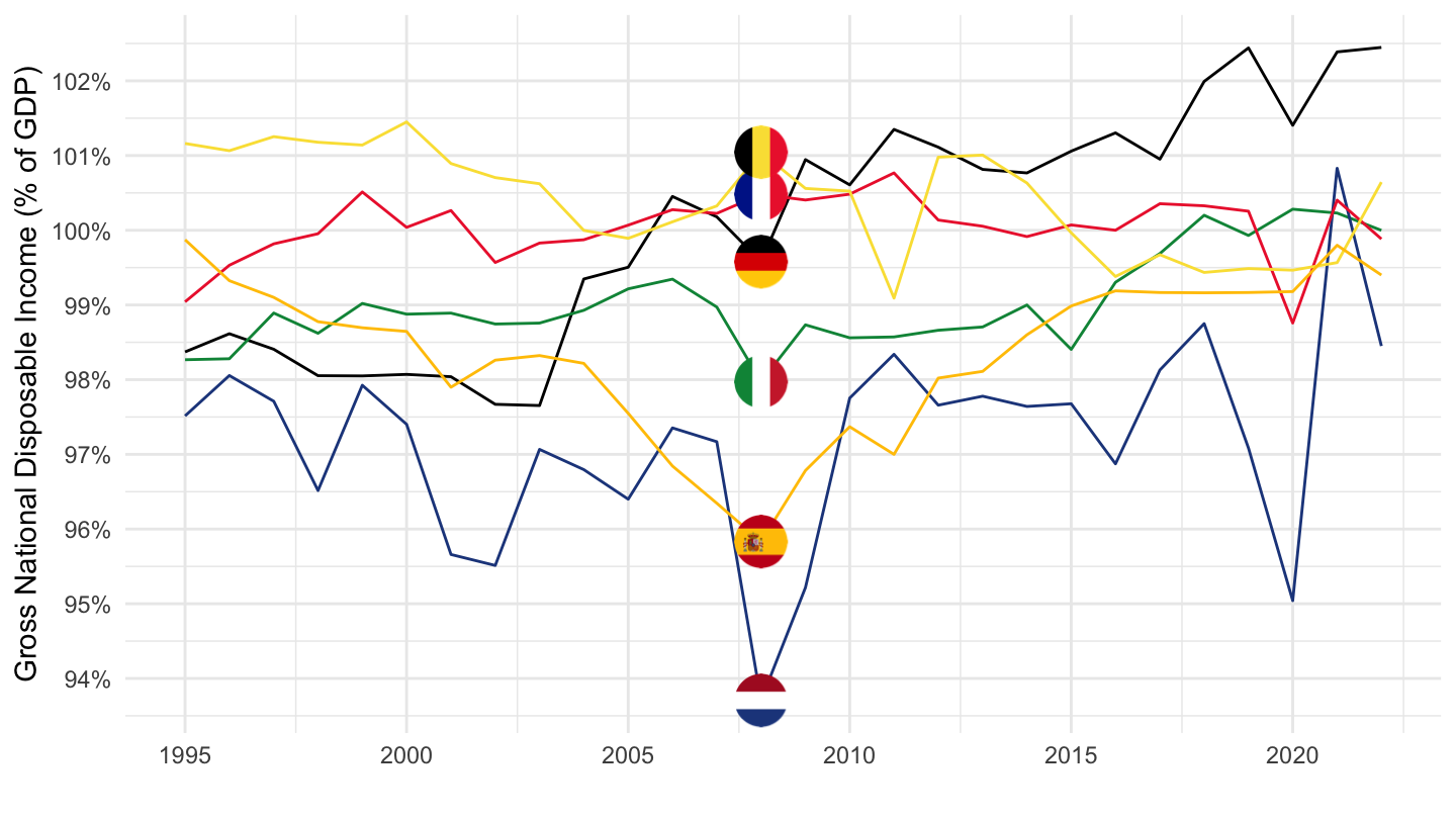
Net capital formation (% of GDP)
All
Code
SNA_TABLE14A %>%
  # NFK1R: Consumption of fixed capital
  # NFP5P: Gross capital formation
  filter(TRANSACT %in% c("NFK1R", "NFP5P", "B1_GE"),
         SECTOR == "S1",
         LOCATION %in% c("FRA", "USA", "DEU", "JPN")) %>%
  left_join(SNA_TABLE14A_var$LOCATION, by = "LOCATION") %>%
  select(Location, TRANSACT, obsTime, obsValue) %>%
  spread(TRANSACT, obsValue) %>%
  na.omit %>%
  year_to_date %>%
  mutate(obsValue = (NFP5P - NFK1R) / B1_GE) %>%
  left_join(colors, by = c("Location" = "country")) %>%
  ggplot() + geom_line(aes(x = date, y = obsValue, color = color)) +
  scale_color_identity() + theme_minimal() + add_4flags +
  scale_x_date(breaks = seq(1920, 2100, 5) %>% paste0("-01-01") %>% as.Date,
               labels = date_format("%Y")) +
  scale_y_continuous(breaks = 0.01*seq(-60, 60, 1),
                     labels = scales::percent_format(accuracy = 1)) +
  ylab("Net Capital Formation (% of GDP)") + xlab("")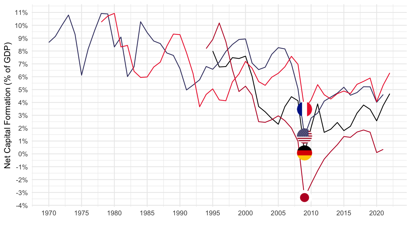
S13
France, United States, Germany
Code
SNA_TABLE14A %>%
  # NFK1R: Consumption of fixed capital
  # NFP5P: Gross capital formation
  filter(TRANSACT %in% c("NFK1R", "NFP5P"),
         SECTOR == "S13",
         LOCATION %in% c("FRA", "USA", "DEU")) %>%
  select(LOCATION, TRANSACT, obsTime, obsValue) %>%
  spread(TRANSACT, obsValue) %>%
  left_join(SNA_TABLE1 %>%
              filter(TRANSACT == "B1_GE",
                     MEASURE == "C") %>%
              select(obsTime, LOCATION, B1_GE = obsValue),
            by = c("LOCATION", "obsTime")) %>%
  left_join(SNA_TABLE14A_var$LOCATION, by = "LOCATION") %>%
  na.omit %>%
  year_to_date %>%
  mutate(obsValue = (NFP5P - NFK1R) / B1_GE) %>%
  filter(date >= as.Date("1995-01-01")) %>%
  left_join(colors, by = c("Location" = "country")) %>%
  mutate(color = ifelse(LOCATION == "USA", color2, color)) %>%
  ggplot() + geom_line(aes(x = date, y = obsValue, color = color)) +
  scale_color_identity() + theme_minimal() + add_3flags +
  scale_x_date(breaks = seq(1920, 2100, 2) %>% paste0("-01-01") %>% as.Date,
               labels = date_format("%Y")) +
  scale_y_continuous(breaks = 0.01*seq(-60, 60, 0.1),
                     labels = scales::percent_format(accuracy = .1)) +
  ylab("Net Capital Formation (% of GDP) - Government") + xlab("") +
  geom_hline(yintercept = 0, linetype = "dashed")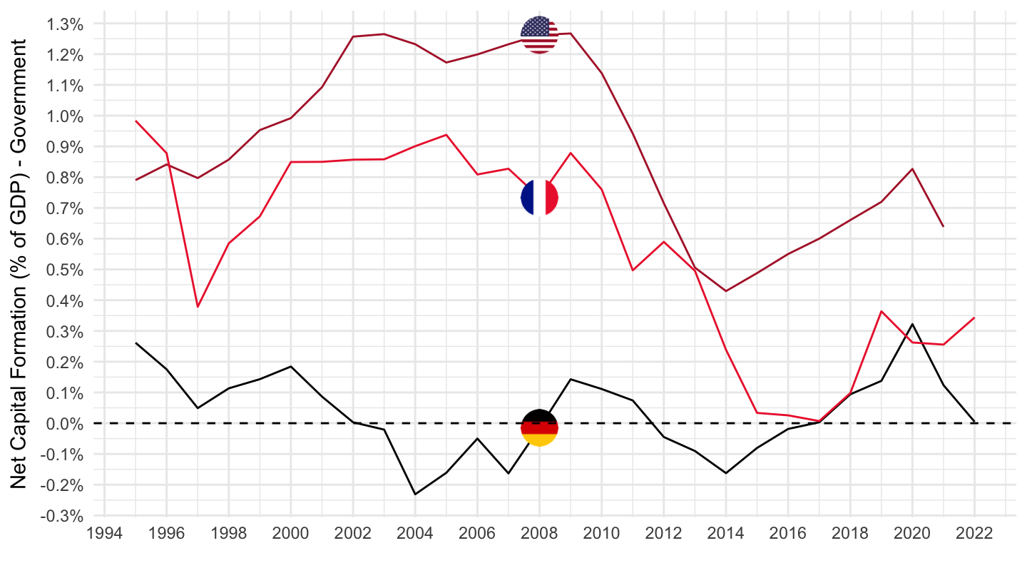
Germany, United States, Germany
Code
SNA_TABLE14A %>%
  # NFK1R: Consumption of fixed capital
  # NFP5P: Gross capital formation
  filter(TRANSACT %in% c("NFK1R", "NFP5P"),
         SECTOR == "S13",
         LOCATION %in% c("DEU", "LVA", "SVK", "CZE")) %>%
  select(LOCATION, TRANSACT, obsTime, obsValue) %>%
  spread(TRANSACT, obsValue) %>%
  left_join(SNA_TABLE1 %>%
              filter(TRANSACT == "B1_GE",
                     MEASURE == "C") %>%
              select(obsTime, LOCATION, B1_GE = obsValue),
            by = c("LOCATION", "obsTime")) %>%
  left_join(SNA_TABLE14A_var$LOCATION, by = "LOCATION") %>%
  na.omit %>%
  year_to_date %>%
  mutate(obsValue = (NFP5P - NFK1R) / B1_GE) %>%
  filter(date >= as.Date("1995-01-01")) %>%
  left_join(colors, by = c("Location" = "country")) %>%
  mutate(color = ifelse(LOCATION == "SVK", "#EE1C25", color)) %>%
  ggplot() + geom_line(aes(x = date, y = obsValue, color = color)) +
  scale_color_identity() + theme_minimal() + add_4flags +
  scale_x_date(breaks = seq(1920, 2100, 5) %>% paste0("-01-01") %>% as.Date,
               labels = date_format("%Y")) +
  scale_y_continuous(breaks = 0.01*seq(-60, 60, 1),
                     labels = scales::percent_format(accuracy = 1)) +
  ylab("Net Capital Formation (% of GDP) - Government") + xlab("") +
  geom_hline(yintercept = 0, linetype = "dashed")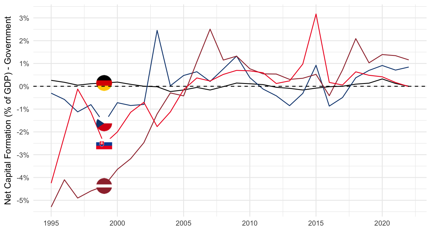
Table
Code
SNA_TABLE14A %>%
  # NFK1R: Consumption of fixed capital
  # NFP5P: Gross capital formation
  filter(TRANSACT %in% c("NFK1R", "NFP5P"),
         SECTOR == "S13") %>%
  select(LOCATION, TRANSACT, obsTime, obsValue) %>%
  spread(TRANSACT, obsValue) %>%
  left_join(SNA_TABLE1 %>%
              filter(TRANSACT == "B1_GE",
                     MEASURE == "C") %>%
              select(obsTime, LOCATION, B1_GE = obsValue),
            by = c("LOCATION", "obsTime")) %>%
  left_join(SNA_TABLE14A_var$LOCATION, by = "LOCATION") %>%
  na.omit %>%
  year_to_date %>%
  mutate(obsValue = (NFP5P - NFK1R) / B1_GE) %>%
  filter(date >= as.Date("1995-01-01"),
         date <= as.Date("2019-01-01")) %>%
  group_by(LOCATION, Location) %>%
  filter(n() == 25) %>%
  summarise(`Avg Net Inv.` = round(100*mean(obsValue), 2)) %>%
  arrange(`Avg Net Inv.`) %>%
  mutate(`Avg Net Inv.` = paste0(`Avg Net Inv.`, " %")) %>%
  mutate(Flag = gsub(" ", "-", str_to_lower(gsub(" ", "-", Location))),
         Flag = paste0('<img src="../../icon/flag/vsmall/', Flag, '.png" alt="Flag">')) %>%
  select(Flag, everything()) %>%
  {if (is_html_output()) datatable(., filter = 'top', rownames = F, escape = F) else .}
Operating surplus and mixed income; gross (% of GDP)
Code
SNA_TABLE14A %>%
  # NFB2G_B3GP: Operating surplus and mixed income
  filter(TRANSACT %in% c("NFB2G_B3GP", "B1_GE"),
         # S1: Total economy
         SECTOR == "S1",
         LOCATION %in% c("FRA", "USA", "DEU", "JPN")) %>%
  left_join(SNA_TABLE14A_var$LOCATION, by = "LOCATION") %>%
  select(Location, TRANSACT, obsTime, obsValue) %>%
  spread(TRANSACT, obsValue) %>%
  na.omit %>%
  year_to_date %>%
  mutate(obsValue = NFB2G_B3GP / B1_GE) %>%
  left_join(colors, by = c("Location" = "country")) %>%
  ggplot() + geom_line(aes(x = date, y = obsValue, color = color)) +
  scale_color_identity() + theme_minimal() + add_4flags +
  scale_x_date(breaks = seq(1920, 2100, 5) %>% paste0("-01-01") %>% as.Date,
               labels = date_format("%Y")) +
  scale_y_continuous(breaks = 0.01*seq(-60, 60, 1),
                     labels = scales::percent_format(accuracy = 1)) +
  ylab("Operating surplus and mixed income (% of GDP)") + xlab("")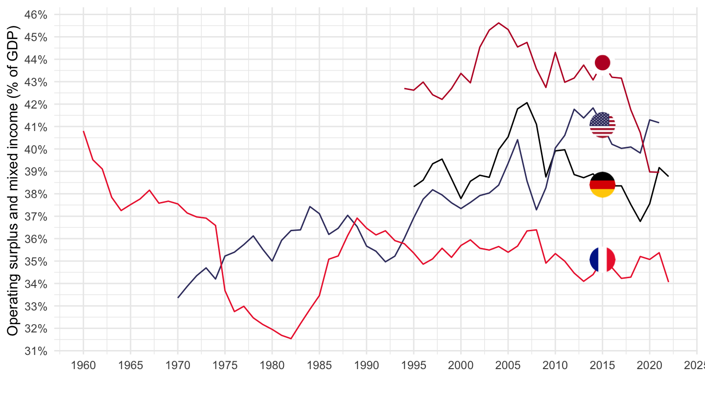
Adjustment for the change in net equity of households in pension funds -
Code
SNA_TABLE14A %>%
  # NFD8P: Adjustment for the change in net equity of households in pension funds
  filter(TRANSACT %in% c("NFD8P", "B1_GE"),
         # S1: Total economy
         SECTOR == "S1",
         LOCATION %in% c("DEU", "USA", "CAN", "JPN")) %>%
  left_join(SNA_TABLE14A_var$LOCATION, by = "LOCATION") %>%
  select(Location, TRANSACT, obsTime, obsValue) %>%
  spread(TRANSACT, obsValue) %>%
  na.omit %>%
  year_to_date %>%
  mutate(obsValue = NFD8P / B1_GE) %>%
  left_join(colors, by = c("Location" = "country")) %>%
  ggplot() + geom_line(aes(x = date, y = obsValue, color = color)) +
  scale_color_identity() + theme_minimal() + add_3flags +
  scale_x_date(breaks = seq(1920, 2100, 5) %>% paste0("-01-01") %>% as.Date,
               labels = date_format("%Y")) +
  scale_y_continuous(breaks = 0.01*seq(-60, 60, 1),
                     labels = scales::percent_format(accuracy = 1)) +
  ylab("Operating surplus and mixed income (% of GDP)") + xlab("")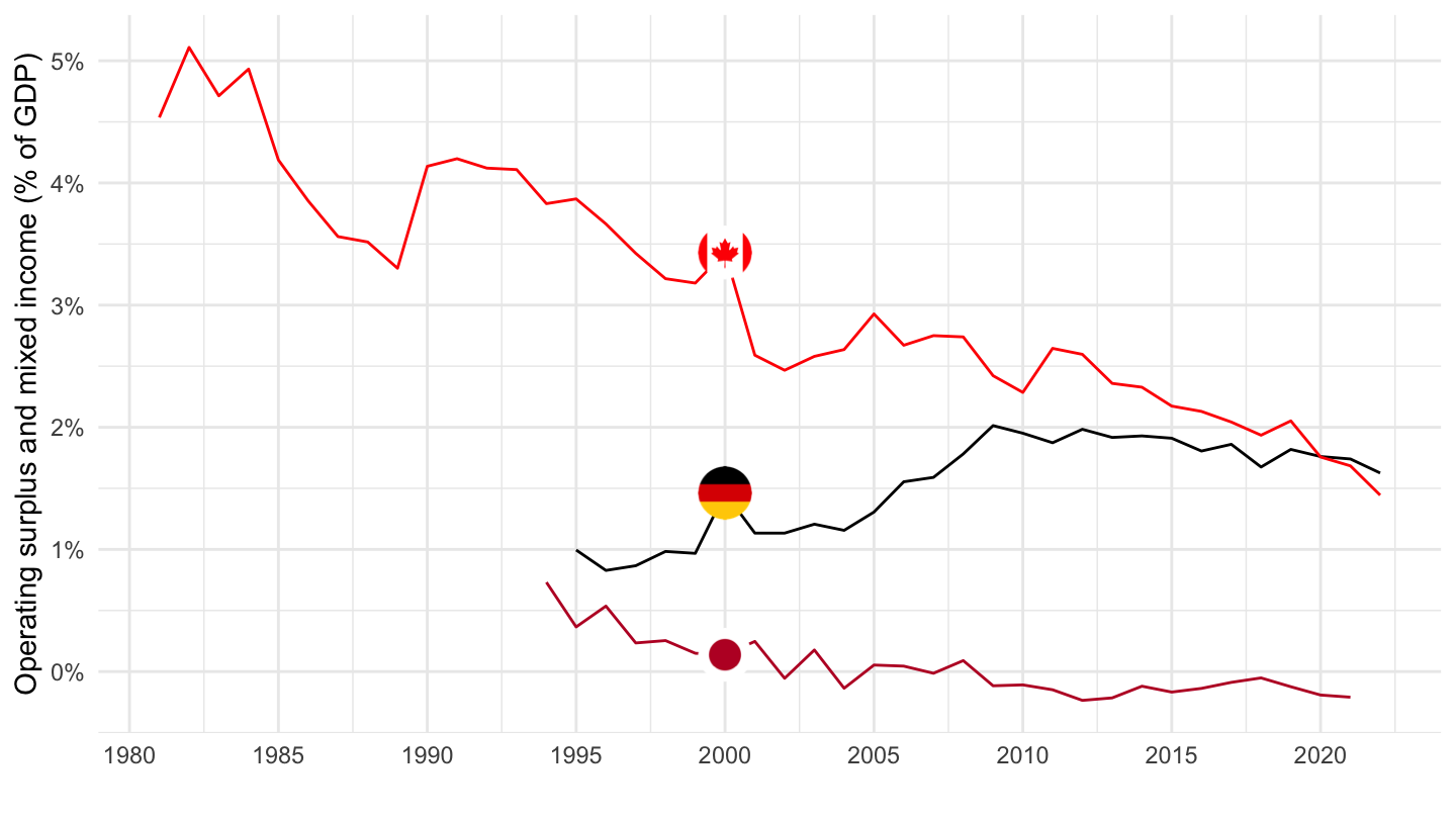
2018
2017 - United States
Code
SNA_TABLE14A %>%
  filter(LOCATION == "USA",
         obsTime == "2017",
         !(SECTOR %in% c("S2", "S14", "S15"))) %>%
  left_join(SNA_TABLE14A_var$TRANSACT, by = "TRANSACT") %>%
  left_join(SNA_TABLE1 %>%
              filter(TRANSACT == "B1_GE",
                     MEASURE == "C") %>%
              select(obsTime, LOCATION, B1_GE = obsValue),
            by = c("LOCATION", "obsTime")) %>%
  mutate(obsValue = round(100*obsValue / B1_GE, 1) %>% paste0(., "%")) %>%
  select(SECTOR, TRANSACT, Transact, obsValue) %>%
  mutate(SECTOR = paste0('<img src="../../icon/sector/vsmall/', SECTOR, '.png" alt="All">')) %>%
  spread(SECTOR, obsValue) %>%
  {if (is_html_output()) datatable(., filter = 'top', rownames = F, escape = F) else .}
2018 - Germany
Code
SNA_TABLE14A %>%
  filter(LOCATION == "DEU",
         obsTime == "2018",
         !(SECTOR %in% c("S2", "S14", "S15"))) %>%
  left_join(SNA_TABLE14A_var$TRANSACT, by = "TRANSACT") %>%
  left_join(SNA_TABLE1 %>%
              filter(TRANSACT == "B1_GE",
                     MEASURE == "C") %>%
              select(obsTime, LOCATION, B1_GE = obsValue),
            by = c("LOCATION", "obsTime")) %>%
  mutate(obsValue = round(100*obsValue / B1_GE, 1) %>% paste0(., "%")) %>%
  select(SECTOR, TRANSACT, Transact, obsValue) %>%
  mutate(SECTOR = paste0('<img src="../../icon/sector/vsmall/', SECTOR, '.png" alt="All">')) %>%
  spread(SECTOR, obsValue) %>%
  {if (is_html_output()) datatable(., filter = 'top', rownames = F, escape = F) else .}
2018 - France
Code
SNA_TABLE14A %>%
  filter(LOCATION == "FRA",
         obsTime == "2018",
         !(SECTOR %in% c("S2", "S14", "S15"))) %>%
  left_join(SNA_TABLE14A_var$TRANSACT, by = "TRANSACT") %>%
  left_join(SNA_TABLE1 %>%
              filter(TRANSACT == "B1_GE",
                     MEASURE == "C") %>%
              select(obsTime, LOCATION, B1_GE = obsValue),
            by = c("LOCATION", "obsTime")) %>%
  mutate(obsValue = round(100*obsValue / B1_GE, 1) %>% paste0(., "%")) %>%
  select(SECTOR, TRANSACT, Transact, obsValue) %>%
  mutate(SECTOR = paste0('<img src="../../icon/sector/vsmall/', SECTOR, '.png" alt="All">')) %>%
  spread(SECTOR, obsValue) %>%
  {if (is_html_output()) datatable(., filter = 'top', rownames = F, escape = F) else .}
2017 - Japan
Code
SNA_TABLE14A %>%
  filter(LOCATION == "JPN",
         obsTime == "2017",
         !(SECTOR %in% c("S2", "S14", "S15"))) %>%
  left_join(SNA_TABLE14A_var$TRANSACT, by = "TRANSACT") %>%
  left_join(SNA_TABLE1 %>%
              filter(TRANSACT == "B1_GE",
                     MEASURE == "C") %>%
              select(obsTime, LOCATION, B1_GE = obsValue),
            by = c("LOCATION", "obsTime")) %>%
  mutate(obsValue = round(100*obsValue / B1_GE, 1) %>% paste0(., "%")) %>%
  select(SECTOR, TRANSACT, Transact, obsValue) %>%
  mutate(SECTOR = paste0('<img src="../../icon/sector/vsmall/', SECTOR, '.png" alt="All">')) %>%
  spread(SECTOR, obsValue) %>%
  {if (is_html_output()) datatable(., filter = 'top', rownames = F, escape = F) else .}
2018 - United Kingdom
Code
SNA_TABLE14A %>%
  filter(LOCATION == "GBR",
         obsTime == "2018",
         !(SECTOR %in% c("S2", "S14", "S15"))) %>%
  left_join(SNA_TABLE14A_var$TRANSACT, by = "TRANSACT") %>%
  left_join(SNA_TABLE1 %>%
              filter(TRANSACT == "B1_GE",
                     MEASURE == "C") %>%
              select(obsTime, LOCATION, B1_GE = obsValue),
            by = c("LOCATION", "obsTime")) %>%
  mutate(obsValue = round(100*obsValue / B1_GE, 1) %>% paste0(., "%")) %>%
  select(SECTOR, TRANSACT, Transact, obsValue) %>%
  mutate(SECTOR = paste0('<img src="../../icon/sector/vsmall/', SECTOR, '.png" alt="All">')) %>%
  spread(SECTOR, obsValue) %>%
  {if (is_html_output()) datatable(., filter = 'top', rownames = F, escape = F) else .}
2016 - China
Code
SNA_TABLE14A %>%
  filter(LOCATION == "CHN",
         obsTime == "2016",
         !(SECTOR %in% c("S2", "S14", "S15"))) %>%
  left_join(SNA_TABLE14A_var$TRANSACT, by = "TRANSACT") %>%
  left_join(SNA_TABLE1 %>%
              filter(TRANSACT == "B1_GE",
                     MEASURE == "C") %>%
              select(obsTime, LOCATION, B1_GE = obsValue),
            by = c("LOCATION", "obsTime")) %>%
  mutate(obsValue = round(100*obsValue / B1_GE, 1) %>% paste0(., "%")) %>%
  select(SECTOR, TRANSACT, Transact, obsValue) %>%
  mutate(SECTOR = paste0('<img src="../../icon/sector/vsmall/', SECTOR, '.png" alt="All">')) %>%
  spread(SECTOR, obsValue) %>%
  {if (is_html_output()) datatable(., filter = 'top', rownames = F, escape = F) else .}