| source | dataset | Title | .html | .rData |
|---|---|---|---|---|
| eurostat | nasq_10_nf_tr | Non-financial transactions | 2026-07-21 | 2026-07-21 |
Non-financial transactions
Data - Eurostat
Info
Data on europe
| source | dataset | Title | .html | .rData |
|---|---|---|---|---|
| eurostat | bop_gdp6_q | Main Balance of Payments and International Investment Position items as share of GDP (BPM6) | 2026-07-21 | 2026-07-21 |
| eurostat | nama_10_a10 | Gross value added and income by A*10 industry breakdowns | 2026-07-21 | 2026-07-21 |
| eurostat | nama_10_a10_e | Employment by A*10 industry breakdowns | 2026-07-21 | 2026-07-21 |
| eurostat | nama_10_gdp | GDP and main components (output, expenditure and income) | 2026-07-21 | 2026-07-21 |
| eurostat | nama_10_lp_ulc | Labour productivity and unit labour costs | 2026-07-21 | 2026-07-21 |
| eurostat | namq_10_a10 | Gross value added and income A*10 industry breakdowns | 2026-07-21 | 2026-07-21 |
| eurostat | namq_10_a10_e | Employment A*10 industry breakdowns | 2026-07-21 | 2026-07-21 |
| eurostat | namq_10_gdp | GDP and main components (output, expenditure and income) | 2026-07-21 | 2026-07-21 |
| eurostat | namq_10_lp_ulc | Labour productivity and unit labour costs | 2026-07-21 | 2026-07-21 |
| eurostat | namq_10_pc | Main GDP aggregates per capita | 2026-07-21 | 2026-07-21 |
| eurostat | nasa_10_nf_tr | Non-financial transactions | 2026-07-21 | 2026-07-21 |
| eurostat | nasq_10_nf_tr | Non-financial transactions | 2026-07-21 | 2026-07-21 |
| eurostat | tipsii40 | Net international investment position - quarterly data, % of GDP | 2026-07-21 | 2026-07-21 |
Info
Exemples
Code
ig_b("eurostat", "nasq_10_nf_tr", "650px-MS_S1M_B6G_20Q4_F")
Last
Code
nasq_10_nf_tr %>%
  group_by(time) %>%
  summarise(Nobs = n()) %>%
  arrange(desc(time)) %>%
  head(2) %>%
print_table_conditional()| time | Nobs |
|---|---|
| 2025Q3 | 29922 |
| 2025Q2 | 29966 |
unit
Code
nasq_10_nf_tr %>%
  left_join(unit, by = "unit") %>%
  group_by(unit, Unit) %>%
  summarise(Nobs = n()) %>%
  arrange(-Nobs) %>%
{if (is_html_output()) print_table(.) else .}| unit | Unit | Nobs |
|---|---|---|
| CP_MNAC | Current prices, million units of national currency | 1788841 |
| CP_MEUR | Current prices, million euro | 1783457 |
sector
Code
nasq_10_nf_tr %>%
  left_join(sector, by = "sector") %>%
  group_by(sector, Sector) %>%
  summarise(Nobs = n()) %>%
  arrange(-Nobs) %>%
{if (is_html_output()) print_table(.) else .}| sector | Sector | Nobs |
|---|---|---|
| S1 | Total economy | 782230 |
| S13 | General government | 722472 |
| S2 | Rest of the world | 635642 |
| S14_S15 | Households; non-profit institutions serving households | 564924 |
| S11 | Non-financial corporations | 427758 |
| S12 | Financial corporations | 391896 |
| S1N | Not sectorised | 45664 |
| S14 | Households | 856 |
| S15 | Non-profit institutions serving households | 856 |
direct
Code
nasq_10_nf_tr %>%
  left_join(direct, by = "direct") %>%
  group_by(direct, Direct) %>%
  summarise(Nobs = n()) %>%
  arrange(-Nobs) %>%
{if (is_html_output()) print_table(.) else .}| direct | Direct | Nobs |
|---|---|---|
| PAID | Paid | 1918500 |
| RECV | Received | 1653798 |
na_item
Code
nasq_10_nf_tr %>%
  left_join(na_item, by = "na_item") %>%
  group_by(na_item, Na_item) %>%
  summarise(Nobs = n()) %>%
  arrange(-Nobs) %>%
  {if (is_html_output()) datatable(., filter = 'top', rownames = F) else .}
s_adj
Code
nasq_10_nf_tr %>%
  left_join(s_adj, by = "s_adj") %>%
  group_by(s_adj, S_adj) %>%
  summarise(Nobs = n()) %>%
  arrange(-Nobs) %>%
{if (is_html_output()) print_table(.) else .}| s_adj | S_adj | Nobs |
|---|---|---|
| NSA | Unadjusted data (i.e. neither seasonally adjusted nor calendar adjusted data) | 3159668 |
| SCA | Seasonally and calendar adjusted data | 412630 |
geo
Code
nasq_10_nf_tr %>%
  left_join(geo, by = "geo") %>%
  group_by(geo, Geo) %>%
  summarise(Nobs = n()) %>%
  arrange(-Nobs) %>%
  mutate(Geo = ifelse(geo == "DE", "Germany", Geo)) %>%
  mutate(Flag = gsub(" ", "-", str_to_lower(Geo)),
         Flag = paste0('<img src="../../bib/flags/vsmasll/', Flag, '.png" alt="Flag">')) %>%
  select(Flag, everything()) %>%
  {if (is_html_output()) datatable(., filter = 'top', rownames = F, escape = F) else .}
Belgium, Luxembourg
All
Code
nasq_10_nf_tr %>%
  filter(geo %in% c("BE", "LU", "FR", "DE", "EA20"),
         na_item %in% c("B2A3G", "B1G"),
         direct == "PAID",
         unit == "CP_MNAC",
         s_adj == "SCA",
         sector == "S11") %>%
  select(geo, time, values, na_item) %>%
  spread(na_item, values) %>%
  mutate(values = B2A3G/B1G) %>%
  quarter_to_date %>%
  filter(date >= as.Date("1995-01-01")) %>%
  left_join(geo, by = "geo") %>%
  mutate(Geo = ifelse(geo == "EA20", "Europe", Geo)) %>%
  left_join(colors, by = c("Geo" = "country")) %>%
  na.omit %>%
  ggplot + theme_minimal() + xlab("") + ylab("% of Gross Value Added") +
  geom_line(aes(x = date, y = values, color = color)) +
  scale_color_identity() + add_4flags +
  scale_x_date(breaks = as.Date(paste0(seq(1940, 2100, 2), "-01-01")),
               labels = date_format("%Y")) +
  scale_y_continuous(breaks = 0.01*seq(0, 100, 1),
                labels = percent_format(a = 1))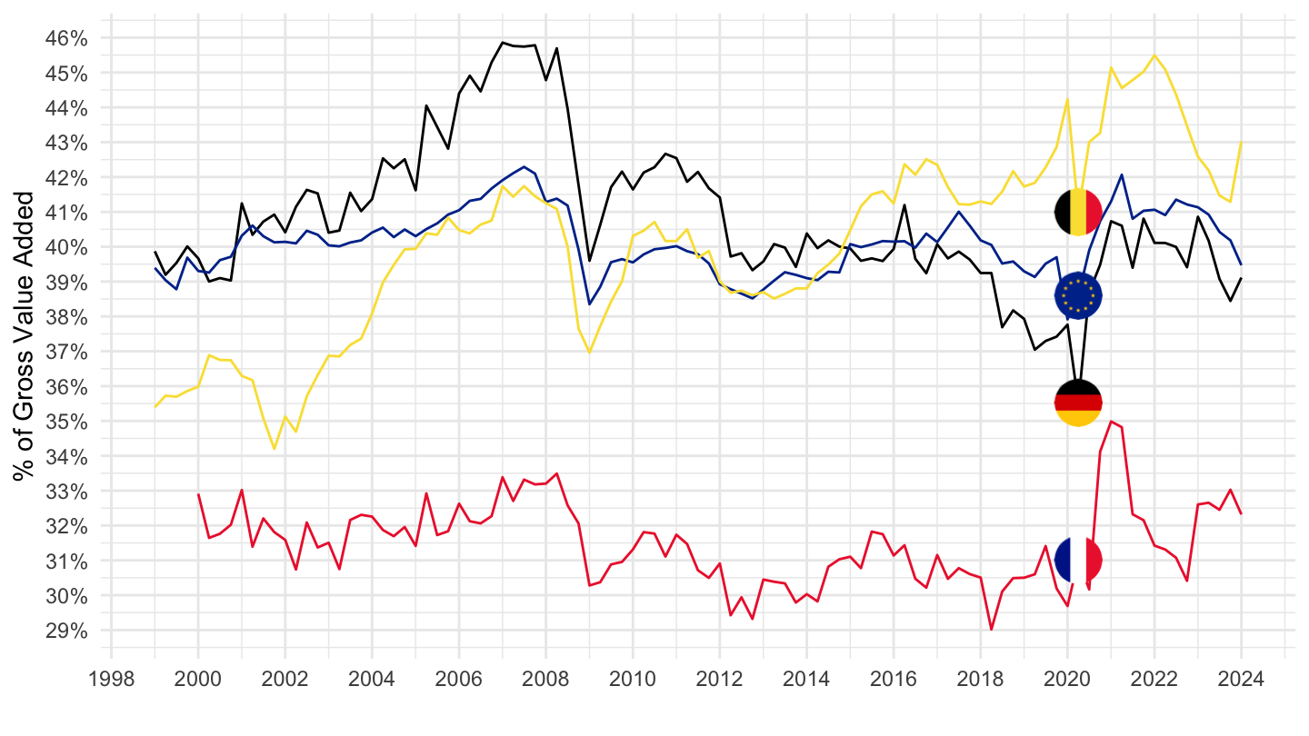
2010
Code
nasq_10_nf_tr %>%
  filter(geo %in% c("BE", "LU", "FR", "DE", "EU"),
         na_item %in% c("B2A3G", "B1G"),
         direct == "PAID",
         unit == "CP_MNAC",
         s_adj == "SCA",
         sector == "S11") %>%
  select(geo, time, values, na_item) %>%
  spread(na_item, values) %>%
  mutate(values = B2A3G/B1G) %>%
  quarter_to_date %>%
  filter(date >= as.Date("2010-01-01")) %>%
  left_join(geo, by = "geo") %>%
  mutate(Geo = ifelse(geo == "EU27_2020", "Europe", Geo)) %>%
  left_join(colors, by = c("Geo" = "country")) %>%
  na.omit %>%
  ggplot + theme_minimal() + xlab("") + ylab("% of Gross Value Added") +
  geom_line(aes(x = date, y = values, color = color)) +
  scale_color_identity() + add_3flags +
  scale_x_date(breaks = as.Date(paste0(seq(1940, 2100, 1), "-01-01")),
               labels = date_format("%Y")) +
  scale_y_continuous(breaks = 0.01*seq(0, 100, 1),
                labels = percent_format(a = 1))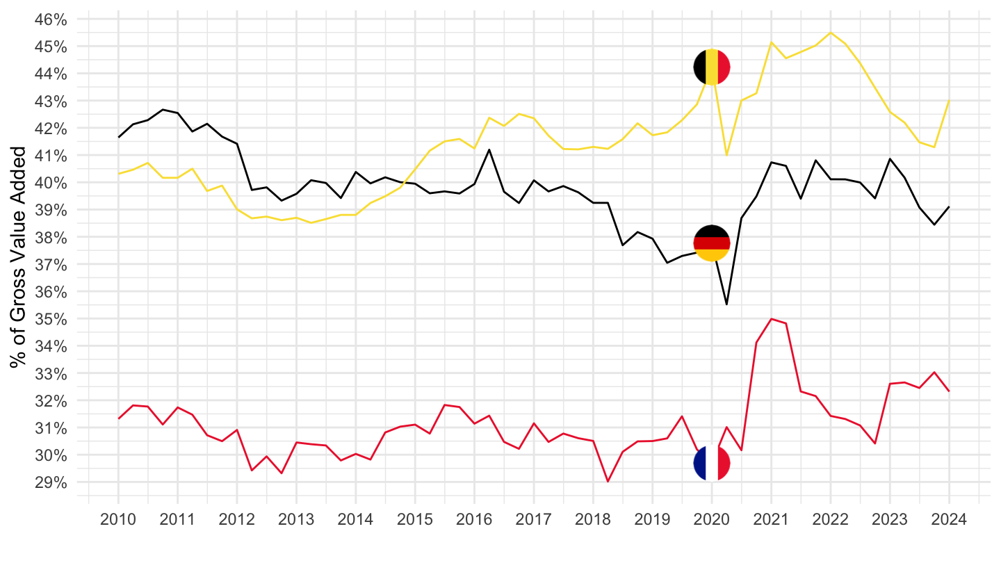
France, Germany, Italy, Spain, Europe
Operating surplus and mixed income, gross - B2A3G, S11
Table
Code
load_data("eurostat/geo.Rdata")
nasq_10_nf_tr %>%
  filter(na_item %in% c("B2A3G", "B1G"),
         direct == "PAID",
         unit == "CP_MNAC",
         s_adj == "SCA",
         sector == "S11",
         time %in% c("2022Q4", "2021Q4", "2019Q4")) %>%
  left_join(geo, by = "geo") %>%
  select(geo, Geo, time, values, na_item) %>%
  spread(na_item, values) %>%
  mutate(values = B2A3G/B1G) %>%
  select(-B2A3G, -B1G) %>%
  spread(time, values) %>%
  mutate(`2021Q4-2022Q4` = `2022Q4` - `2021Q4`,
         `2019Q4-2022Q4` = `2022Q4` - `2019Q4`) %>%
  arrange(-`2019Q4-2022Q4`) %>%
print_table_conditional| geo | Geo | 2019Q4 | 2021Q4 | 2022Q4 | 2021Q4-2022Q4 | 2019Q4-2022Q4 |
|---|---|---|---|---|---|---|
| NO | Norway | 0.4849330 | 0.6270687 | 0.6506859 | 0.0236173 | 0.1657529 |
| EL | Greece | 0.3612532 | 0.3851922 | 0.4423141 | 0.0571219 | 0.0810609 |
| IE | Ireland | 0.7419825 | 0.7692043 | 0.7860535 | 0.0168492 | 0.0440710 |
| NL | Netherlands | 0.3995201 | 0.4453739 | 0.4390383 | -0.0063356 | 0.0395181 |
| DK | Denmark | 0.4165516 | 0.4682542 | 0.4514557 | -0.0167984 | 0.0349042 |
| BE | Belgium | 0.4260504 | 0.4395690 | 0.4536718 | 0.0141028 | 0.0276214 |
| IT | Italy | 0.4341158 | 0.4497484 | 0.4609823 | 0.0112339 | 0.0268666 |
| PL | Poland | 0.4632065 | 0.4588402 | 0.4896984 | 0.0308582 | 0.0264919 |
| DE | Germany | 0.3696053 | 0.4036642 | 0.3958101 | -0.0078541 | 0.0262048 |
| EU27_2020 | European Union - 27 countries (from 2020) | 0.4022970 | 0.4205540 | 0.4203093 | -0.0002448 | 0.0180123 |
| EA20 | Euro area – 20 countries (2023-2025) | 0.3969039 | 0.4147475 | 0.4147827 | 0.0000352 | 0.0178788 |
| CZ | Czechia | 0.4490720 | 0.4328376 | 0.4661602 | 0.0333226 | 0.0170882 |
| EE | Estonia | 0.4462676 | 0.4563201 | 0.4549820 | -0.0013381 | 0.0087144 |
| PT | Portugal | 0.3810113 | 0.3511777 | 0.3882752 | 0.0370975 | 0.0072639 |
| FR | France | 0.3041358 | 0.3104757 | 0.3100233 | -0.0004524 | 0.0058874 |
| FI | Finland | 0.4154136 | 0.4305972 | 0.4198151 | -0.0107820 | 0.0044015 |
| ES | Spain | 0.4116541 | 0.3847911 | 0.4098811 | 0.0250900 | -0.0017731 |
| AT | Austria | 0.4072503 | 0.4058683 | 0.4049872 | -0.0008812 | -0.0022632 |
| SE | Sweden | 0.3703256 | 0.3837890 | 0.3604524 | -0.0233366 | -0.0098733 |
| RO | Romania | 0.5243758 | 0.5393794 | 0.5140056 | -0.0253738 | -0.0103702 |
| HU | Hungary | 0.4459074 | 0.4415773 | 0.4174265 | -0.0241508 | -0.0284809 |
| UK | United Kingdom | 0.3694683 | NA | NA | NA | NA |
All
Code
nasq_10_nf_tr %>%
  filter(geo %in% c("FR", "DE", "IT", "ES", "EA20"),
         na_item == "B2A3G",
         direct == "PAID",
         unit == "CP_MNAC",
         s_adj == "NSA",
         sector == "S11") %>%
  select(geo, time, values, sector) %>%
  left_join(gdp, by = c("geo", "time")) %>%
  mutate(values = values/gdp) %>%
  quarter_to_date %>%
  left_join(geo, by = "geo") %>%
  mutate(Geo = ifelse(geo == "EA20", "Europe", Geo)) %>%
  left_join(colors, by = c("Geo" = "country")) %>%
  na.omit %>%
  ggplot + theme_minimal() + xlab("") + ylab("") +
  geom_line(aes(x = date, y = values, color = color)) +
  scale_color_identity() + add_5flags +
  scale_x_date(breaks = as.Date(paste0(seq(1940, 2100, 10), "-01-01")),
               labels = date_format("%Y")) +
  scale_y_continuous(breaks = 0.01*seq(0, 100, 1),
                labels = percent_format(a = 1))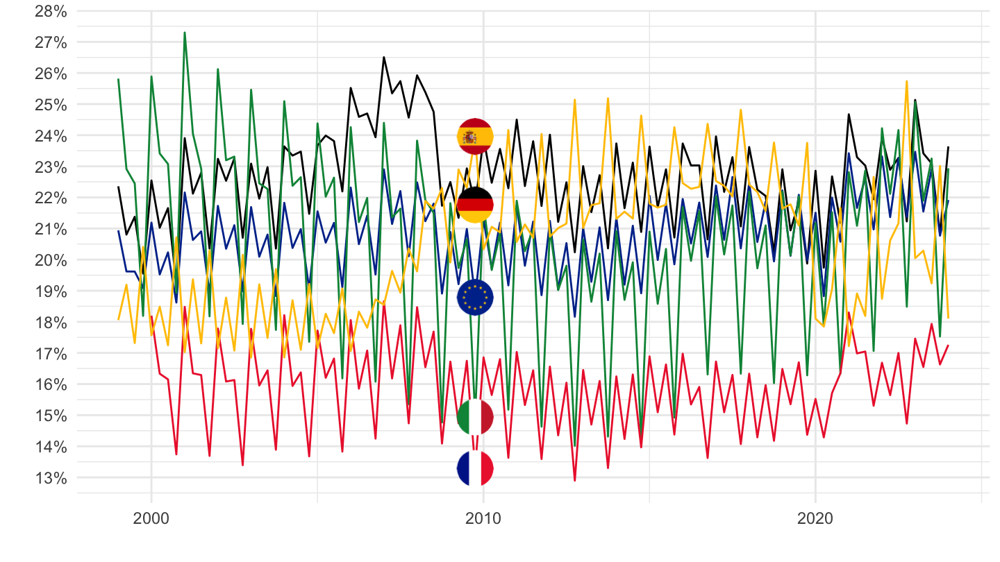
1998-
Code
nasq_10_nf_tr %>%
  filter(geo %in% c("FR", "DE", "IT", "ES", "EA20"),
         na_item == "B2A3G",
         direct == "PAID",
         unit == "CP_MNAC",
         s_adj == "NSA",
         sector == "S11") %>%
  select(geo, time, values, sector) %>%
  left_join(gdp, by = c("geo", "time")) %>%
  mutate(values = values/gdp) %>%
  quarter_to_date %>%
  filter(date >= as.Date("1998-01-01")) %>%
  left_join(geo, by = "geo") %>%
  mutate(Geo = ifelse(geo == "EA20", "Europe", Geo)) %>%
  left_join(colors, by = c("Geo" = "country")) %>%
  na.omit %>%
  ggplot + theme_minimal() + xlab("") + ylab("") +
  geom_line(aes(x = date, y = values, color = color)) +
  scale_color_identity() + add_5flags +
  scale_x_date(breaks = as.Date(paste0(seq(1940, 2100, 2), "-01-01")),
               labels = date_format("%Y")) +
  scale_y_continuous(breaks = 0.01*seq(0, 100, 1),
                labels = percent_format(a = 1))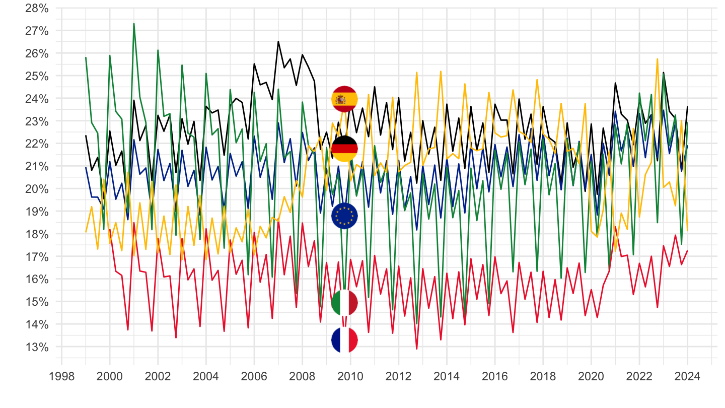
2010-
NSA
Code
nasq_10_nf_tr %>%
  filter(geo %in% c("FR", "DE", "IT", "ES", "EA20"),
         na_item == "B2A3G",
         direct == "PAID",
         unit == "CP_MNAC",
         s_adj == "NSA",
         sector == "S11") %>%
  select(geo, time, values, sector) %>%
  left_join(gdp, by = c("geo", "time")) %>%
  mutate(values = values/gdp) %>%
  quarter_to_date %>%
  filter(date >= as.Date("2010-01-01")) %>%
  left_join(geo, by = "geo") %>%
  mutate(Geo = ifelse(geo == "EA20", "Europe", Geo)) %>%
  left_join(colors, by = c("Geo" = "country")) %>%
  na.omit %>%
  ggplot + theme_minimal() + xlab("") + ylab("") +
  geom_line(aes(x = date, y = values, color = color)) +
  scale_color_identity() + add_5flags +
  scale_x_date(breaks = as.Date(paste0(seq(1940, 2100, 1), "-01-01")),
               labels = date_format("%Y")) +
  scale_y_continuous(breaks = 0.01*seq(0, 100, 1),
                labels = percent_format(a = 1))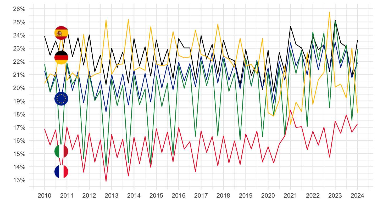
SCA
PAID
% of GDP
Code
nasq_10_nf_tr %>%
  filter(geo %in% c("FR", "DE", "IT", "ES", "EA20"),
         na_item == "B2A3G",
         direct == "PAID",
         unit == "CP_MNAC",
         s_adj == "SCA",
         sector == "S11") %>%
  select(geo, time, values, sector) %>%
  left_join(gdp, by = c("geo", "time")) %>%
  mutate(values = values/gdp) %>%
  quarter_to_date %>%
  filter(date >= as.Date("2010-01-01")) %>%
  left_join(geo, by = "geo") %>%
  mutate(Geo = ifelse(geo == "EA20", "Europe", Geo)) %>%
  left_join(colors, by = c("Geo" = "country")) %>%
  na.omit %>%
  ggplot + theme_minimal() + xlab("") + ylab("% of GDP") +
  geom_line(aes(x = date, y = values, color = color)) +
  scale_color_identity() + add_5flags +
  scale_x_date(breaks = as.Date(paste0(seq(1940, 2100, 1), "-01-01")),
               labels = date_format("%Y")) +
  scale_y_continuous(breaks = 0.01*seq(0, 100, 1),
                labels = percent_format(a = 1))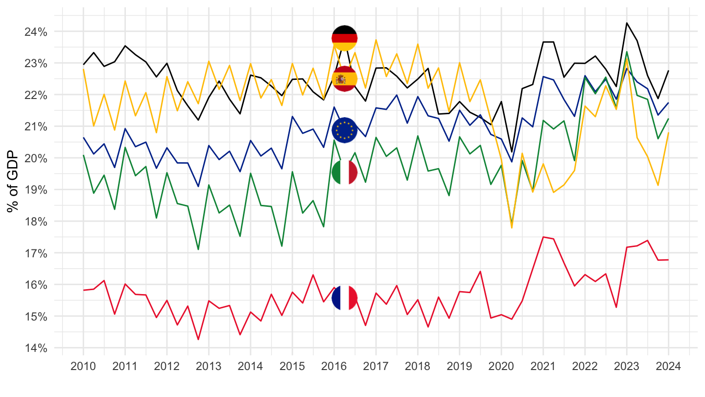
% of Gross Value Added (GVA)
All
Code
nasq_10_nf_tr %>%
  filter(geo %in% c("FR", "DE", "IT", "ES", "EA20"),
         na_item %in% c("B2A3G", "B1G"),
         direct == "PAID",
         unit == "CP_MNAC",
         s_adj == "SCA",
         sector == "S11") %>%
  select(geo, time, values, na_item) %>%
  spread(na_item, values) %>%
  mutate(values = B2A3G/B1G) %>%
  quarter_to_date %>%
  filter(date >= as.Date("1995-01-01")) %>%
  left_join(geo, by = "geo") %>%
  mutate(Geo = ifelse(geo == "EA20", "Europe", Geo)) %>%
  left_join(colors, by = c("Geo" = "country")) %>%
  na.omit %>%
  ggplot + theme_minimal() + xlab("") + ylab("% of Gross Value Added") +
  geom_line(aes(x = date, y = values, color = color)) +
  scale_color_identity() + add_5flags +
  scale_x_date(breaks = as.Date(paste0(seq(1940, 2100, 2), "-01-01")),
               labels = date_format("%Y")) +
  scale_y_continuous(breaks = 0.01*seq(0, 100, 1),
                labels = percent_format(a = 1))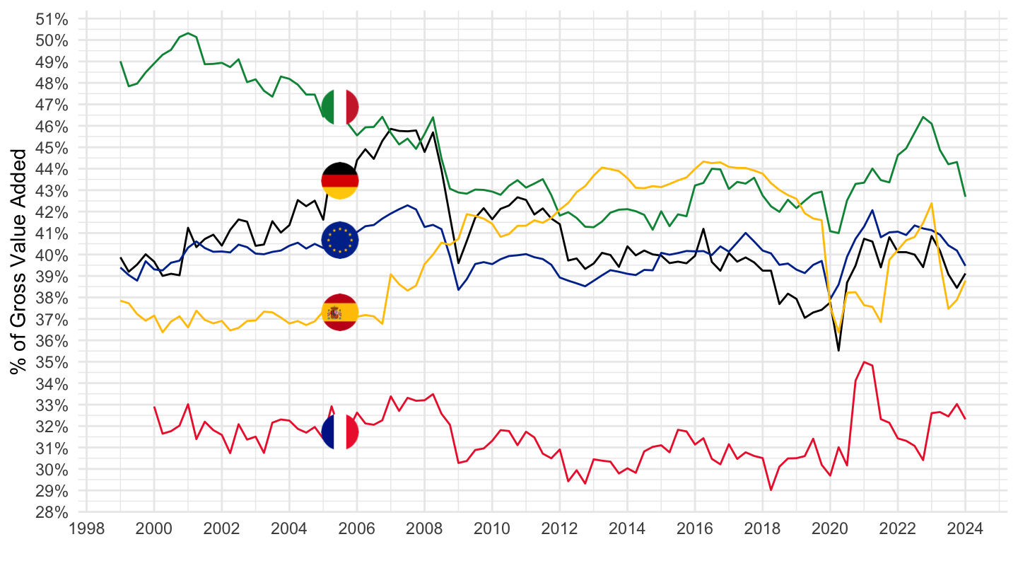
2010-
Code
nasq_10_nf_tr %>%
  filter(geo %in% c("FR", "DE", "IT", "ES", "EA20"),
         na_item %in% c("B2A3G", "B1G"),
         direct == "PAID",
         unit == "CP_MNAC",
         s_adj == "SCA",
         sector == "S11") %>%
  select(geo, time, values, na_item) %>%
  spread(na_item, values) %>%
  mutate(values = B2A3G/B1G) %>%
  quarter_to_date %>%
  filter(date >= as.Date("2010-01-01")) %>%
  left_join(geo, by = "geo") %>%
  mutate(Geo = ifelse(geo == "EA20", "Europe", Geo)) %>%
  left_join(colors, by = c("Geo" = "country")) %>%
  # na.omit %>%
  ggplot + theme_minimal() + xlab("") + ylab("% of GDP") +
  geom_line(aes(x = date, y = values, color = color)) +
  scale_color_identity() + add_5flags +
  scale_x_date(breaks = as.Date(paste0(seq(1940, 2100, 1), "-01-01")),
               labels = date_format("%Y")) +
  scale_y_continuous(breaks = 0.01*seq(0, 100, 1),
                labels = percent_format(a = 1))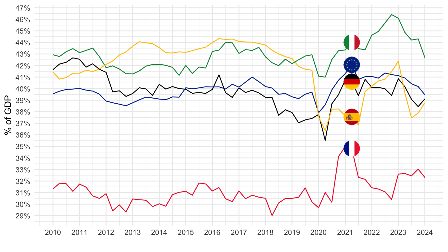
2014-
Code
load_data("eurostat/geo_fr.Rdata")
geo_fr <- geo %>%
  setNames(c("geo", "Geo_fr"))
load_data("eurostat/geo.Rdata")
nasq_10_nf_tr %>%
  filter(geo %in% c("FR", "DE", "IT", "ES", "EA20"),
         na_item %in% c("B2A3G", "B1G"),
         direct == "PAID",
         unit == "CP_MNAC",
         s_adj == "SCA",
         sector == "S11") %>%
  select(geo, time, values, na_item) %>%
  spread(na_item, values) %>%
  mutate(values = B2A3G/B1G) %>%
  quarter_to_date %>%
  filter(date >= as.Date("2014-01-01")) %>%
  left_join(geo, by = "geo") %>%
  left_join(geo_fr, by = "geo") %>%
  mutate(Geo = ifelse(geo == "EA20", "Europe", Geo)) %>%
  left_join(colors, by = c("Geo" = "country")) %>%
  na.omit %>%
  ggplot + theme_minimal() + xlab("") + ylab("% of GDP") +
  geom_line(aes(x = date, y = values, color = color, linetype = Geo_fr)) +
  scale_color_identity() + add_5flags +
  scale_x_date(breaks = as.Date(paste0(seq(1940, 2100, 1), "-01-01")),
               labels = date_format("%Y")) +
  scale_y_continuous(breaks = 0.01*seq(0, 100, 1),
                labels = percent_format(a = 1)) +
  theme(legend.position = c(0.55, 0.50),
        legend.title = element_blank())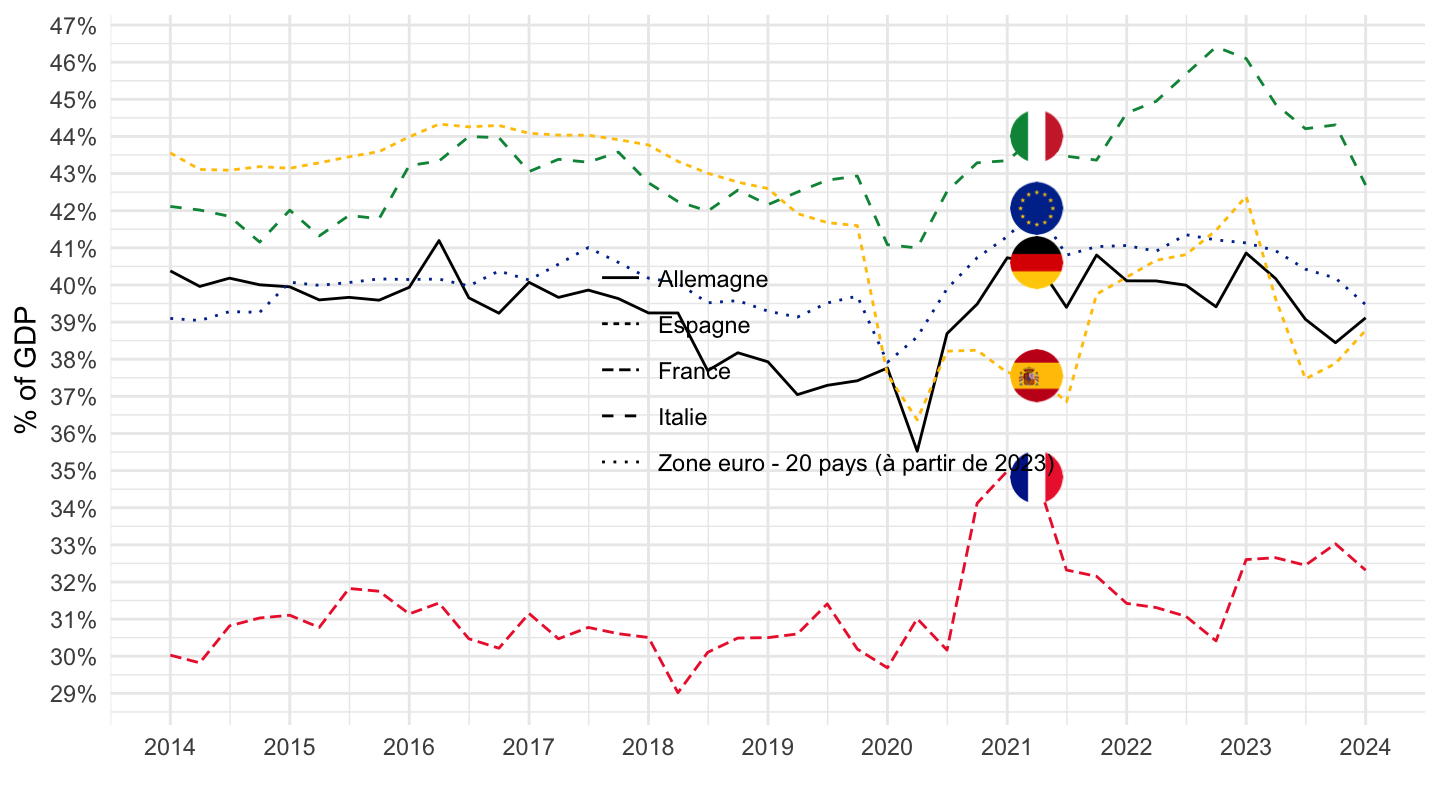
2017-
Code
load_data("eurostat/geo_fr.Rdata")
geo_fr <- geo %>%
  setNames(c("geo", "Geo_fr"))
load_data("eurostat/geo.Rdata")
nasq_10_nf_tr %>%
  filter(geo %in% c("FR", "DE", "IT", "ES", "EA20"),
         na_item %in% c("B2A3G", "B1G"),
         direct == "PAID",
         unit == "CP_MNAC",
         s_adj == "SCA",
         sector == "S11") %>%
  select(geo, time, values, na_item) %>%
  spread(na_item, values) %>%
  mutate(values = B2A3G/B1G) %>%
  quarter_to_date %>%
  filter(date >= as.Date("2017-01-01")) %>%
  left_join(geo, by = "geo") %>%
  left_join(geo_fr, by = "geo") %>%
  mutate(Geo = ifelse(geo == "EA20", "Europe", Geo)) %>%
  left_join(colors, by = c("Geo" = "country")) %>%
  na.omit %>%
  ggplot(.) + theme_minimal() + xlab("") + ylab("B2A3G/B1G (% of GDP)") +
  geom_line(aes(x = date, y = values, color = color)) +
  scale_color_identity() + add_5flags +
  scale_x_date(breaks = as.Date(paste0(seq(1940, 2100, 1), "-01-01")),
               labels = date_format("%Y")) +
  scale_y_continuous(breaks = 0.01*seq(0, 100, 1),
                labels = percent_format(a = 1)) +
  theme(legend.position = c(0.55, 0.50),
        legend.title = element_blank()) +
  geom_text_repel(data = . %>%
                    group_by(geo) %>%
                    filter(date %in% c(as.Date("2017-01-01"),
                                       as.Date("2020-01-01"),
                                       max(date))),
            aes(x = date, y = values, color = color, label = percent(values, acc = 0.01)))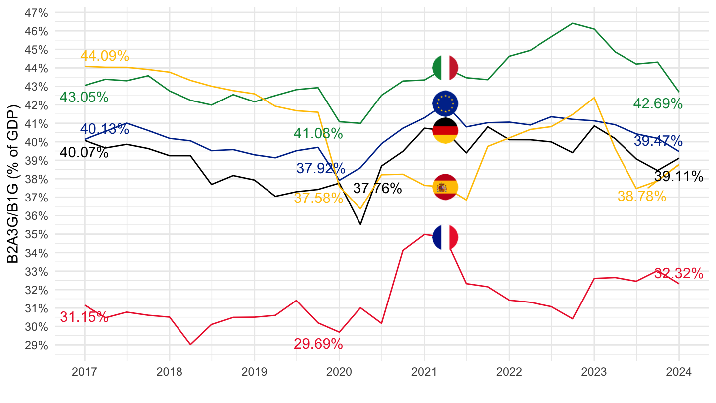
2017-
Code
load_data("eurostat/geo_fr.Rdata")
geo_fr <- geo %>%
  setNames(c("geo", "Geo_fr")) %>%
  mutate(Geo_fr = ifelse(geo == "DE", "Allemagne", Geo_fr),
         Geo_fr = ifelse(geo == "EA20", "Zone Euro", Geo_fr))
load_data("eurostat/geo.Rdata")
load_data("eurostat/na_item_fr.Rdata")
nasq_10_nf_tr %>%
  filter(geo %in% c("FR", "DE", "IT", "ES", "EA20"),
         na_item %in% c("B2A3G", "B1G"),
         direct == "PAID",
         unit == "CP_MNAC",
         s_adj == "SCA",
         sector == "S11") %>%
  select(geo, time, values, na_item) %>%
  spread(na_item, values) %>%
  mutate(values = B2A3G/B1G) %>%
  quarter_to_date %>%
  filter(date >= as.Date("2017-01-01")) %>%
  left_join(geo, by = "geo") %>%
  left_join(geo_fr, by = "geo") %>%
  mutate(Geo = ifelse(geo == "EA20", "Europe", Geo)) %>%
  left_join(colors, by = c("Geo" = "country")) %>%
  na.omit %>%
  ggplot + theme_minimal() + xlab("") + ylab("Excédent d'exploitation et revenu mixte (% du PIB)") +
  geom_line(aes(x = date, y = values, color = color, linetype = Geo_fr)) +
  scale_color_identity() + add_5flags +
  scale_x_date(breaks = as.Date(paste0(seq(1940, 2100, 1), "-01-01")),
               labels = date_format("%Y")) +
  scale_y_continuous(breaks = 0.01*seq(0, 100, 1),
                labels = percent_format(a = 1)) +
  theme(legend.position = c(0.1, 0.4),
        legend.title = element_blank())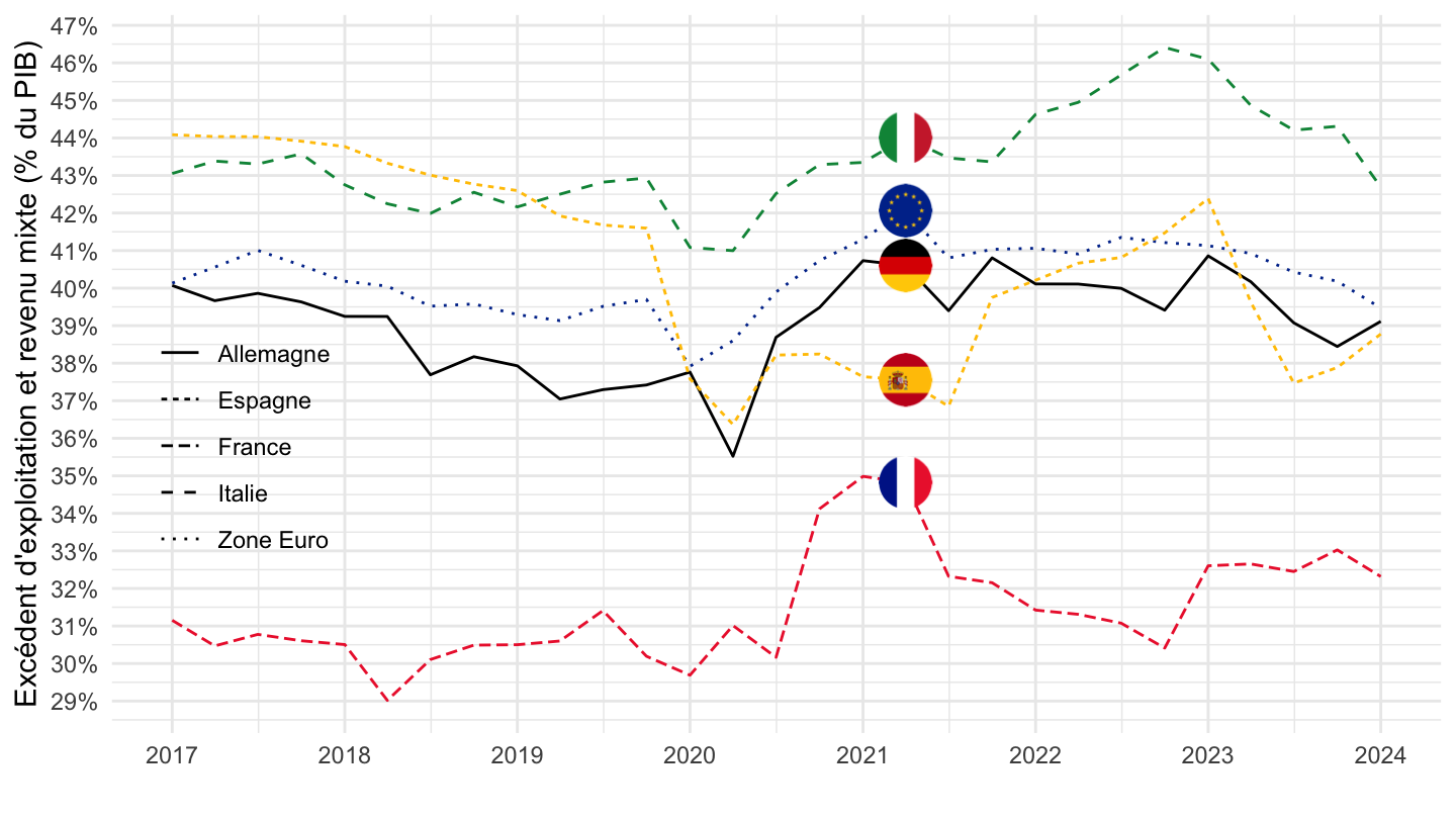
RECV
Code
nasq_10_nf_tr %>%
  filter(geo %in% c("FR", "DE", "IT", "ES", "EA20"),
         na_item == "B2A3G",
         direct == "RECV",
         unit == "CP_MNAC",
         s_adj == "SCA",
         sector == "S11") %>%
  select(geo, time, values, sector) %>%
  left_join(gdp, by = c("geo", "time")) %>%
  mutate(values = values/gdp) %>%
  quarter_to_date %>%
  filter(date >= as.Date("2010-01-01")) %>%
  left_join(geo, by = "geo") %>%
  mutate(Geo = ifelse(geo == "EA20", "Europe", Geo)) %>%
  left_join(colors, by = c("Geo" = "country")) %>%
  na.omit %>%
  ggplot + theme_minimal() + xlab("") + ylab("% of GDP") +
  geom_line(aes(x = date, y = values, color = color)) +
  scale_color_identity() + add_5flags +
  scale_x_date(breaks = as.Date(paste0(seq(1940, 2100, 1), "-01-01")),
               labels = date_format("%Y")) +
  scale_y_continuous(breaks = 0.01*seq(0, 100, 1),
                labels = percent_format(a = 1))
2017-
Code
nasq_10_nf_tr %>%
  filter(geo %in% c("FR", "DE", "IT", "ES", "EA20"),
         na_item == "B2A3G",
         direct == "PAID",
         unit == "CP_MNAC",
         s_adj == "NSA",
         sector == "S11") %>%
  select(geo, time, values, sector) %>%
  left_join(gdp, by = c("geo", "time")) %>%
  mutate(values = values/gdp) %>%
  quarter_to_date %>%
  filter(date >= as.Date("2017-01-01")) %>%
  left_join(geo, by = "geo") %>%
  mutate(Geo = ifelse(geo == "EA20", "Europe", Geo)) %>%
  left_join(colors, by = c("Geo" = "country")) %>%
  na.omit %>%
  ggplot + theme_minimal() + xlab("") + ylab("") +
  geom_line(aes(x = date, y = values, color = color)) +
  scale_color_identity() + add_5flags +
  scale_x_date(breaks = as.Date(paste0(seq(1940, 2100, 1), "-01-01")),
               labels = date_format("%Y")) +
  scale_y_continuous(breaks = 0.01*seq(0, 100, 1),
                labels = percent_format(a = 1))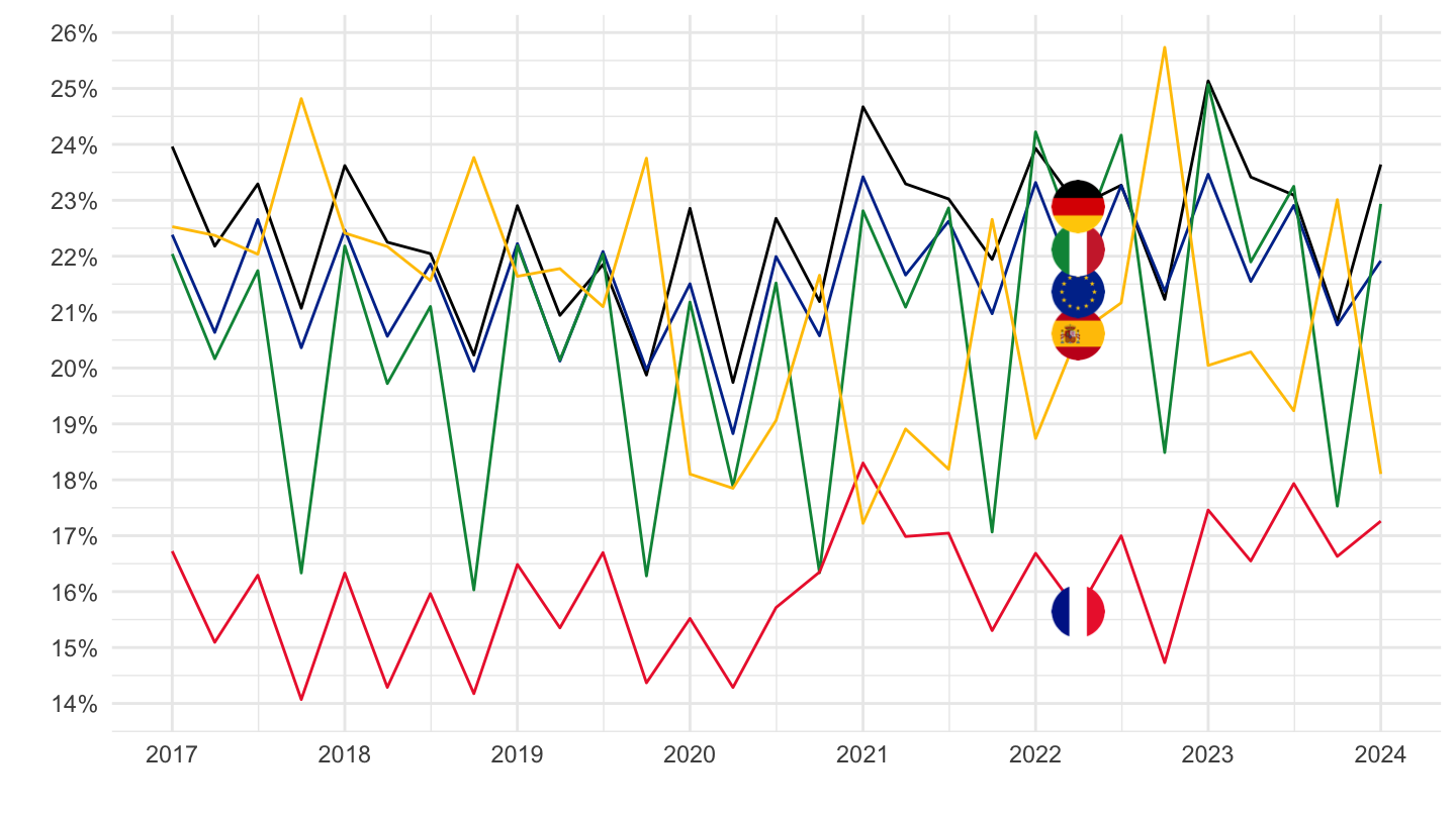
Net lending / Borrowing: financial saving rate (B9)
France, Germany, Italy, Spain
B9
B9
Code
nasq_10_nf_tr %>%
  filter(geo %in% c("FR"),
         na_item == "B9",
         s_adj == "NSA",
         #direct == "PAID",
         unit == "CP_MNAC") %>%
  left_join(sector, by = "sector") %>%
  left_join(gdp_adj, by = c("geo", "time", "s_adj")) %>%
  mutate(values = values/gdp) %>%
  quarter_to_date %>%
  left_join(geo, by = "geo") %>%
  mutate(Geo = ifelse(geo == "EA20", "Europe", Geo)) %>%
  left_join(colors, by = c("Geo" = "country")) %>%
  filter(date >= as.Date("1999-01-01")) %>%
  arrange(desc(date)) %>%
  select(date, values, Sector, direct) %>%
  ggplot + theme_minimal() + xlab("") + ylab("% of GDP") +
  geom_line(aes(x = date, y = values, color = Sector, linetype = direct)) +
  theme(legend.position = c(0.3, 0.8),
        legend.title = element_blank()) +
  scale_x_date(breaks = as.Date(paste0(seq(1940, 2100, 2), "-01-01")),
               labels = date_format("%Y")) +
  scale_y_continuous(breaks = 0.01*seq(-100, 100, 1),
                labels = percent_format(a = 1))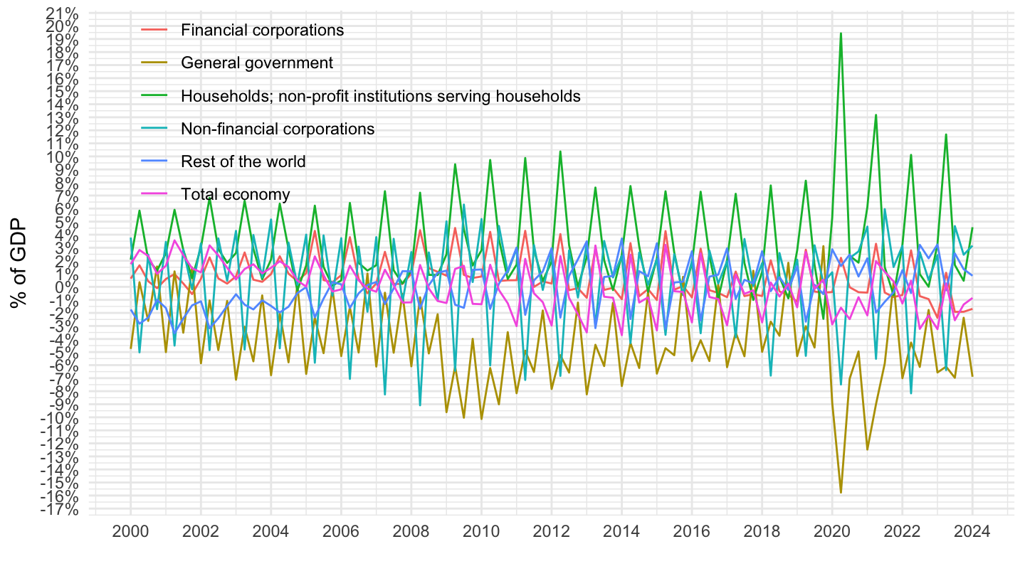
1999-
% of GDP
Code
nasq_10_nf_tr %>%
  filter(geo %in% c("FR", "DE", "IT", "ES", "EA20"),
         na_item == "B9",
         #s_adj == "SCA",
         #direct == "PAID",
         unit == "CP_MNAC",
         sector %in% c("S14_S15")) %>%
  select(geo, time, values, sector) %>%
  left_join(namq_10_gdp_B1GQ_NSA_CPMNAC, by = c("geo", "time")) %>%
  mutate(values = values/B1GQ_NSA_CPMNAC) %>%
  quarter_to_date %>%
  left_join(geo, by = "geo") %>%
  mutate(Geo = ifelse(geo == "EA20", "Europe", Geo)) %>%
  left_join(colors, by = c("Geo" = "country")) %>%
  filter(date >= as.Date("1999-01-01")) %>%
  ggplot + theme_minimal() + xlab("") + ylab("% of GDP") +
  geom_line(aes(x = date, y = values, color = color)) +
  scale_color_identity() + add_5flags +
  scale_x_date(breaks = as.Date(paste0(seq(1940, 2100, 2), "-01-01")),
               labels = date_format("%Y")) +
  scale_y_continuous(breaks = 0.01*seq(-100, 100, 1),
                labels = percent_format(a = 1))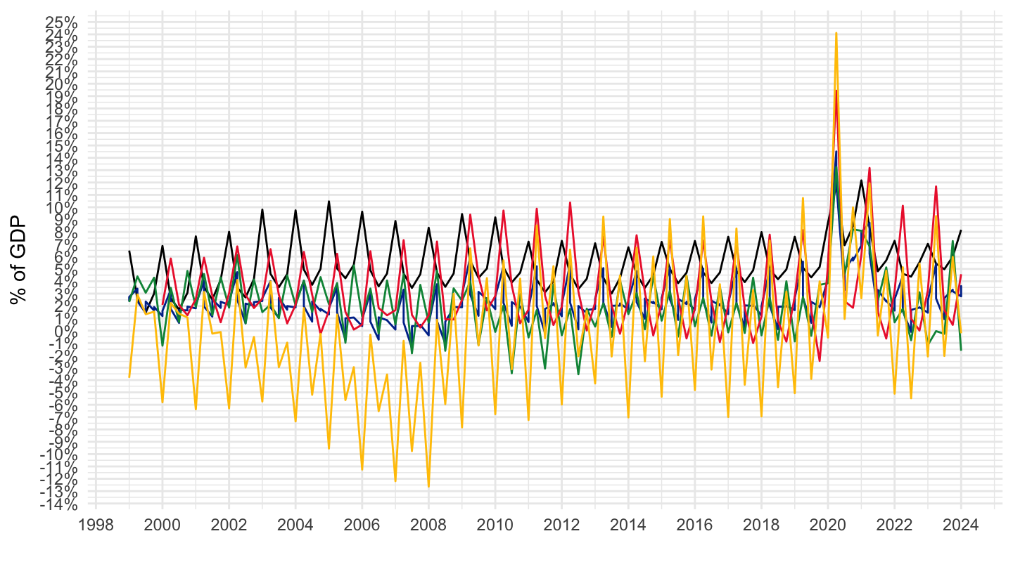
1999-
% of GDP
Code
nasq_10_nf_tr %>%
  filter(geo %in% c("FR", "DE", "IT", "ES", "EA20"),
         na_item == "B9",
         s_adj == "SCA",
         #direct == "PAID",
         unit == "CP_MNAC",
         sector %in% c("S13")) %>%
  select(geo, time, values, sector) %>%
  left_join(namq_10_gdp_B1GQ_NSA_CPMNAC, by = c("geo", "time")) %>%
  mutate(values = values/B1GQ_NSA_CPMNAC) %>%
  quarter_to_date %>%
  left_join(geo, by = "geo") %>%
  mutate(Geo = ifelse(geo == "EA20", "Europe", Geo)) %>%
  left_join(colors, by = c("Geo" = "country")) %>%
  filter(date >= as.Date("1999-01-01")) %>%
  ggplot + theme_minimal() + xlab("") + ylab("% of GDP") +
  geom_line(aes(x = date, y = values, color = color)) +
  scale_color_identity() + add_5flags +
  scale_x_date(breaks = as.Date(paste0(seq(1940, 2100, 2), "-01-01")),
               labels = date_format("%Y")) +
  scale_y_continuous(breaks = 0.01*seq(-100, 100, 1),
                labels = percent_format(a = 1))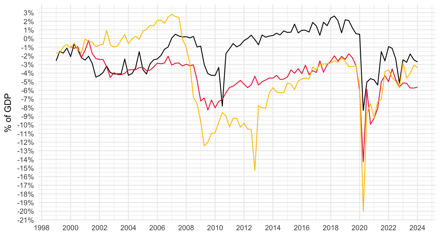
Saving Rate (B8G)
France, Germany, Italy, Spain
All
Code
nasq_10_nf_tr %>%
  filter(geo %in% c("FR", "DE", "IT", "ES"),
         na_item == "B8G",
         s_adj == "SCA",
         direct == "PAID",
         unit == "CP_MNAC",
         sector == "S14_S15") %>%
  select(geo, time, values, sector) %>%
  left_join(namq_10_gdp_B1GQ_NSA_CPMNAC, by = c("geo", "time")) %>%
  mutate(values = values/B1GQ_NSA_CPMNAC) %>%
  quarter_to_date %>%
  left_join(geo, by = "geo") %>%
  left_join(colors, by = c("Geo" = "country")) %>%
  ggplot + theme_minimal() + xlab("") + ylab("% of GDP") +
  geom_line(aes(x = date, y = values, color = color)) +
  scale_color_identity() + add_4flags +
  scale_x_date(breaks = as.Date(paste0(seq(1940, 2100, 10), "-01-01")),
               labels = date_format("%Y")) +
  scale_y_continuous(breaks = 0.01*seq(0, 100, 1),
                labels = percent_format(a = 1))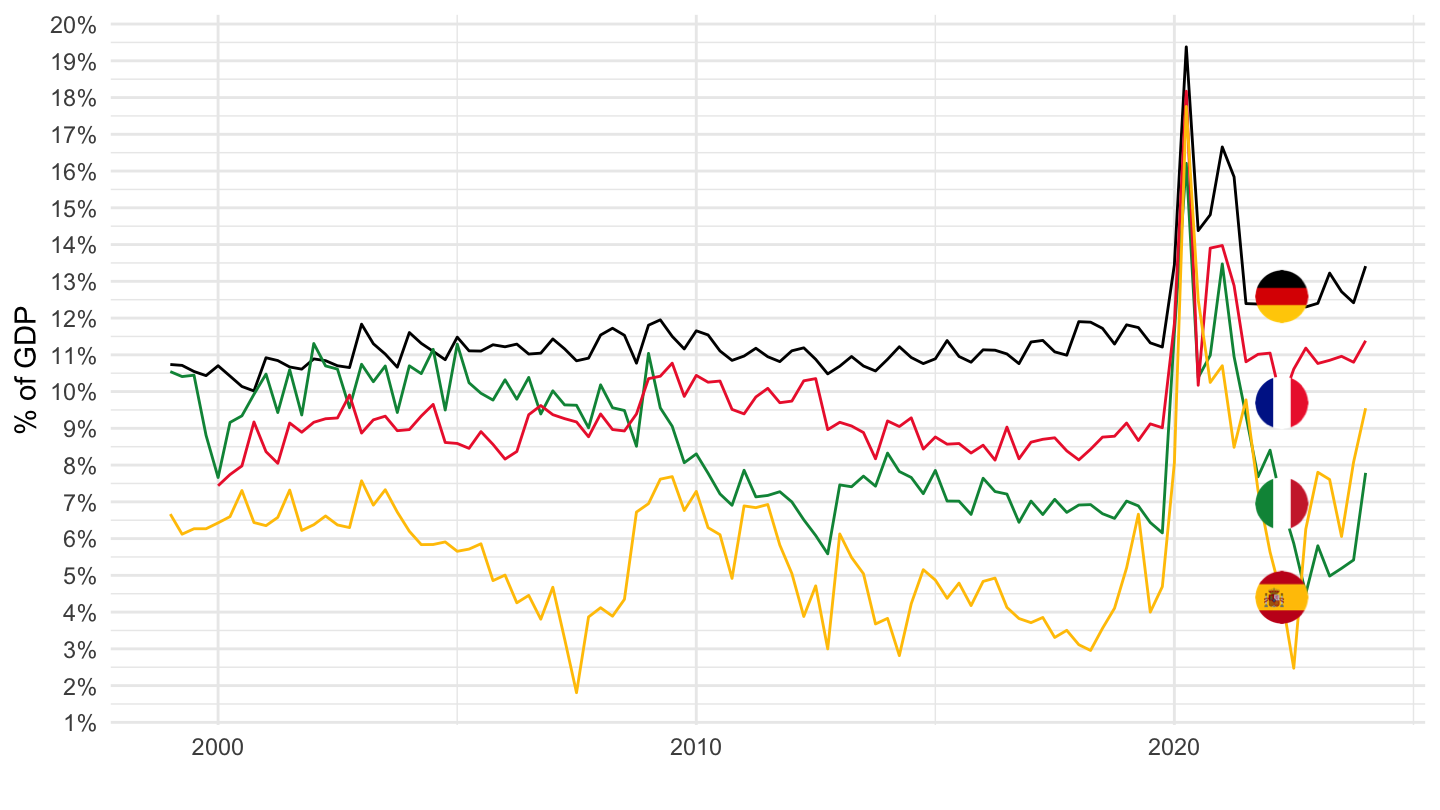
1999-
% of GDP
Code
nasq_10_nf_tr %>%
  filter(geo %in% c("FR", "DE", "IT", "ES", "EA20"),
         na_item == "B8G",
         s_adj == "SCA",
         direct == "PAID",
         unit == "CP_MNAC",
         sector == "S14_S15") %>%
  select(geo, time, values, sector) %>%
  left_join(namq_10_gdp_B1GQ_NSA_CPMNAC, by = c("geo", "time")) %>%
  mutate(values = values/B1GQ_NSA_CPMNAC) %>%
  quarter_to_date %>%
  left_join(geo, by = "geo") %>%
  mutate(Geo = ifelse(geo == "EA20", "Europe", Geo)) %>%
  left_join(colors, by = c("Geo" = "country")) %>%
  filter(date >= as.Date("1999-01-01")) %>%
  ggplot + theme_minimal() + xlab("") + ylab("% of GDP") +
  geom_line(aes(x = date, y = values, color = color)) +
  scale_color_identity() + add_5flags +
  scale_x_date(breaks = as.Date(paste0(seq(1940, 2100, 2), "-01-01")),
               labels = date_format("%Y")) +
  scale_y_continuous(breaks = 0.01*seq(0, 100, 1),
                labels = percent_format(a = 1))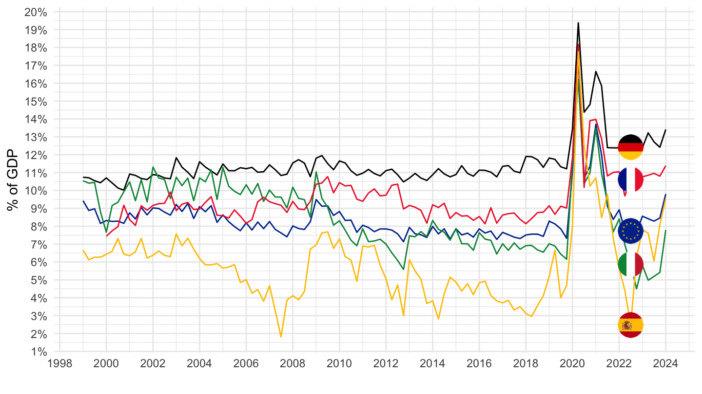
% of Disposable income
Code
nasq_10_nf_tr %>%
  filter(geo %in% c("FR", "DE", "IT", "ES", "EA20"),
         na_item %in% c("B8G", "B6G"),
         s_adj == "SCA",
         direct == "PAID",
         unit == "CP_MNAC",
         sector == "S14_S15") %>%
  select(geo, time, values, sector, na_item) %>%
  spread(na_item, values) %>%
  mutate(values = B8G/B6G) %>%
  quarter_to_date %>%
  left_join(geo, by = "geo") %>%
  mutate(Geo = ifelse(geo == "EA20", "Europe", Geo)) %>%
  left_join(colors, by = c("Geo" = "country")) %>%
  filter(date >= as.Date("1999-01-01")) %>%
  ggplot + theme_minimal() + xlab("") + ylab("B8G/B6G (% of Disposable income)") +
  geom_line(aes(x = date, y = values, color = color)) +
  scale_color_identity() + add_5flags +
  scale_x_date(breaks = as.Date(paste0(seq(1940, 2100, 2), "-01-01")),
               labels = date_format("%Y")) +
  scale_y_continuous(breaks = 0.01*seq(0, 100, 2),
                labels = percent_format(a = 1))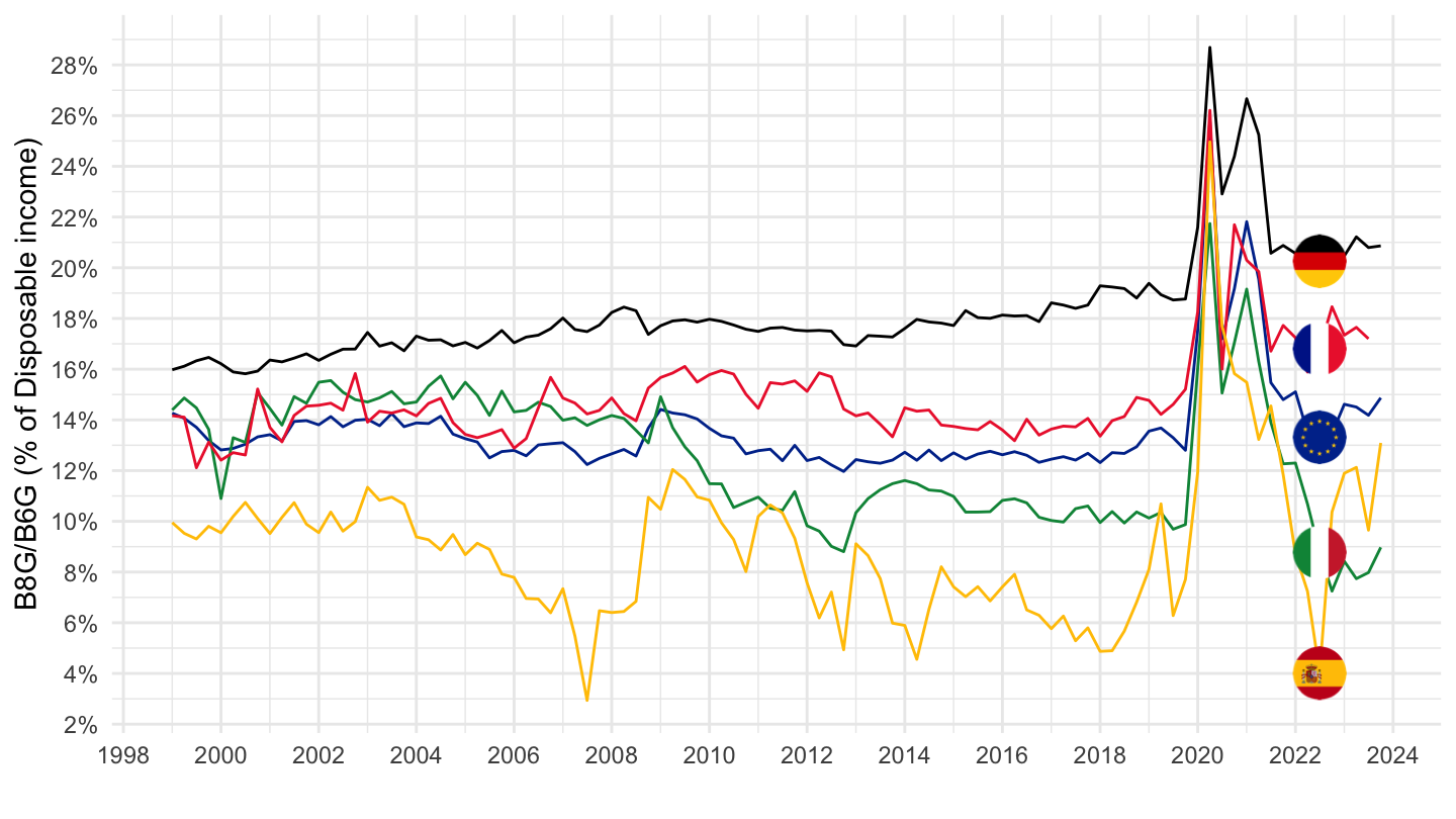
2000-
% of GDP
Code
nasq_10_nf_tr %>%
  filter(geo %in% c("FR", "DE", "IT", "ES", "EA20"),
         na_item == "B8G",
         s_adj == "SCA",
         direct == "PAID",
         unit == "CP_MNAC",
         sector == "S14_S15") %>%
  select(geo, time, values, sector) %>%
  left_join(namq_10_gdp_B1GQ_NSA_CPMNAC, by = c("geo", "time")) %>%
  mutate(values = values/B1GQ_NSA_CPMNAC) %>%
  quarter_to_date %>%
  left_join(geo, by = "geo") %>%
  mutate(Geo = ifelse(geo == "EA20", "Europe", Geo)) %>%
  left_join(colors, by = c("Geo" = "country")) %>%
  filter(date >= as.Date("2000-01-01")) %>%
  ggplot + theme_minimal() + xlab("") + ylab("% of GDP") +
  geom_line(aes(x = date, y = values, color = color)) +
  scale_color_identity() + add_5flags +
  scale_x_date(breaks = as.Date(paste0(seq(1940, 2100, 2), "-01-01")),
               labels = date_format("%Y")) +
  scale_y_continuous(breaks = 0.01*seq(0, 100, 1),
                labels = percent_format(a = 1))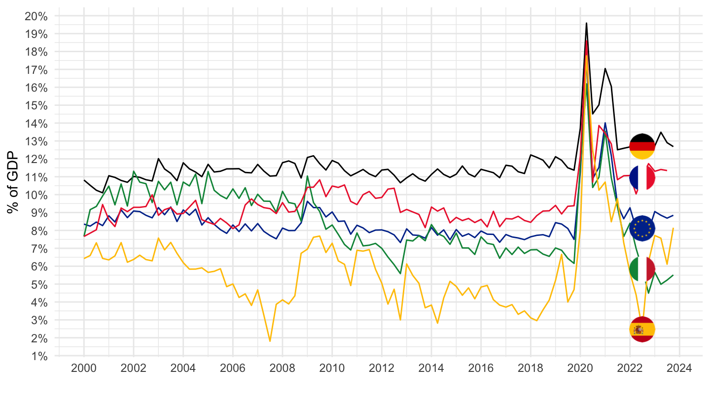
% of Disposable income
Code
nasq_10_nf_tr %>%
  filter(geo %in% c("FR", "DE", "IT", "ES", "EA20"),
         na_item %in% c("B8G", "B6G"),
         s_adj == "SCA",
         direct == "PAID",
         unit == "CP_MNAC",
         sector == "S14_S15") %>%
  select(geo, time, values, sector, na_item) %>%
  spread(na_item, values) %>%
  mutate(values = B8G/B6G) %>%
  quarter_to_date %>%
  left_join(geo, by = "geo") %>%
  mutate(Geo = ifelse(geo == "EA20", "Europe", Geo)) %>%
  left_join(colors, by = c("Geo" = "country")) %>%
  filter(date >= as.Date("2000-01-01")) %>%
  ggplot + theme_minimal() + xlab("") + ylab("B8G/B6G (% of Disposable income)") +
  geom_line(aes(x = date, y = values, color = color)) +
  scale_color_identity() + add_5flags +
  scale_x_date(breaks = as.Date(paste0(seq(1940, 2100, 2), "-01-01")),
               labels = date_format("%Y")) +
  scale_y_continuous(breaks = 0.01*seq(0, 100, 2),
                labels = percent_format(a = 1))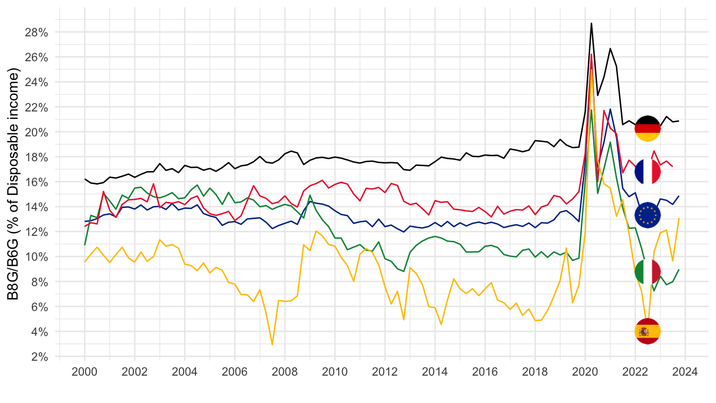
2015-
Code
nasq_10_nf_tr %>%
  filter(geo %in% c("FR", "DE", "IT", "ES", "EA20"),
         na_item == "B8G",
         s_adj == "SCA",
         direct == "PAID",
         unit == "CP_MNAC",
         sector == "S14_S15") %>%
  select(geo, time, values, sector) %>%
  left_join(namq_10_gdp_B1GQ_NSA_CPMNAC, by = c("geo", "time")) %>%
  mutate(values = values/B1GQ_NSA_CPMNAC) %>%
  quarter_to_date %>%
  left_join(geo, by = "geo") %>%
  mutate(Geo = ifelse(geo == "EA20", "Europe", Geo)) %>%
  left_join(colors, by = c("Geo" = "country")) %>%
  filter(date >= as.Date("2015-01-01")) %>%
  ggplot + theme_minimal() + xlab("") + ylab("% of GDP") +
  geom_line(aes(x = date, y = values, color = color)) +
  scale_color_identity() + add_5flags +
  scale_x_date(breaks = as.Date(paste0(seq(1940, 2100, 1), "-01-01")),
               labels = date_format("%Y")) +
  scale_y_continuous(breaks = 0.01*seq(0, 100, 1),
                labels = percent_format(a = 1))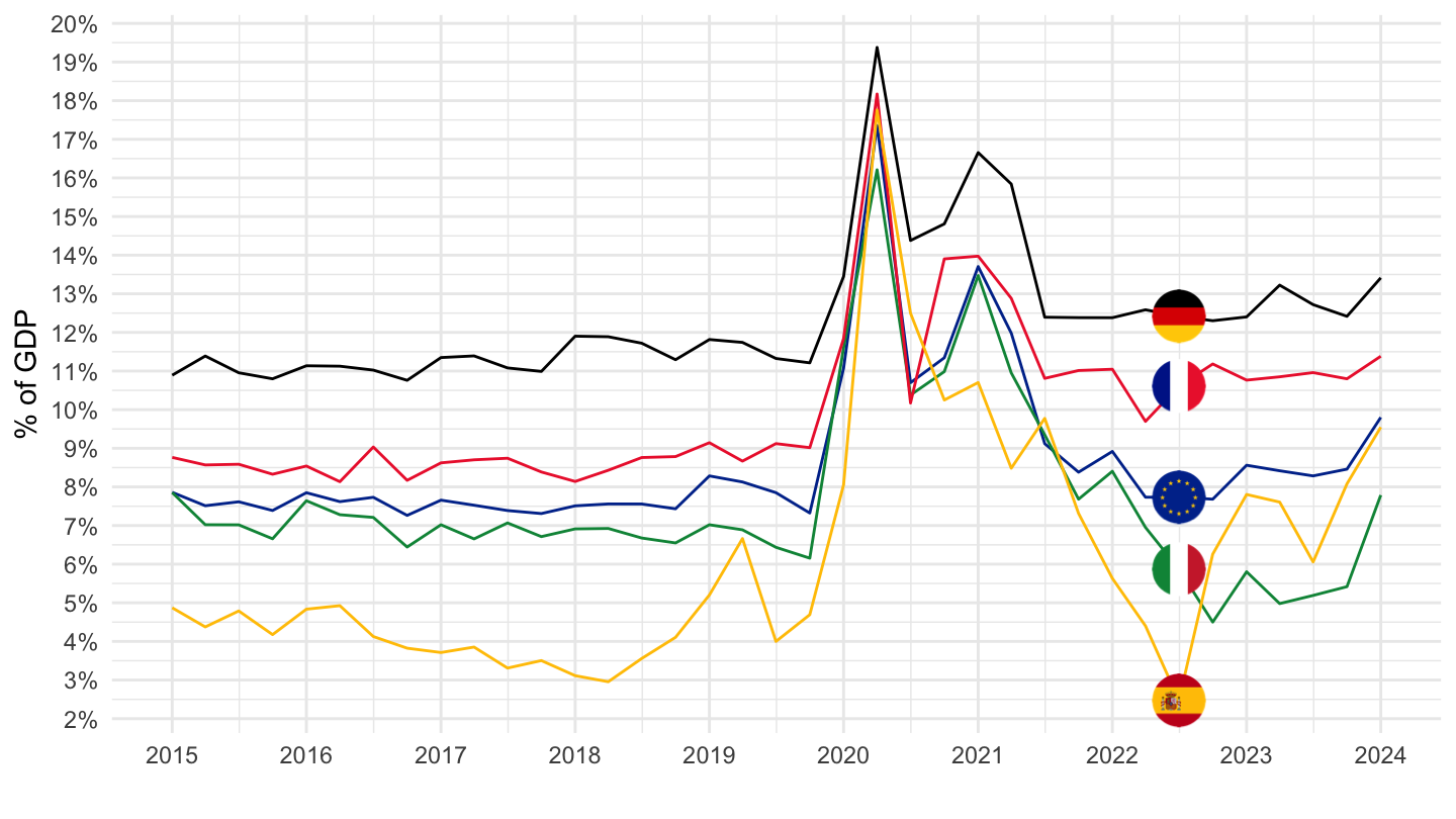
Operating surplus and mixed income, gross
Code
nasq_10_nf_tr %>%
  filter(geo %in% c("FR", "DE", "IT"),
         # B2A3G: Operating surplus and mixed income, gross
         na_item == "B2A3G",
         # SCA: Seasonally and calendar adjusted data
         s_adj == "SCA",
         # PAID: Paid
         direct == "PAID",
         # CP_MNAC: Current prices, million units of national currency
         unit == "CP_MNAC",
         # S1: Total economy
         sector == "S1") %>%
  quarter_to_date %>%
  left_join(geo, by = "geo") %>%
  ggplot + geom_line(aes(x = date, y = values/1000, color = Geo, linetype = Geo)) +
  scale_color_manual(values = viridis(4)[1:3]) +
  theme_minimal()  +
  scale_x_date(breaks = as.Date(paste0(seq(1940, 2100, 5), "-01-01")),
               labels = date_format("%Y")) +
  theme(legend.position = c(0.3, 0.85),
        legend.title = element_blank()) +
  xlab("") + ylab("") +
  scale_y_log10(breaks = c(c(1, 2, 3, 5, 8, 10), 10*c(1, 2, 3, 5, 8, 10), 100*c(1, 2, 3, 5, 8, 10)),
                labels = dollar_format(suffix = " Bn€", prefix = "", accuracy = 1))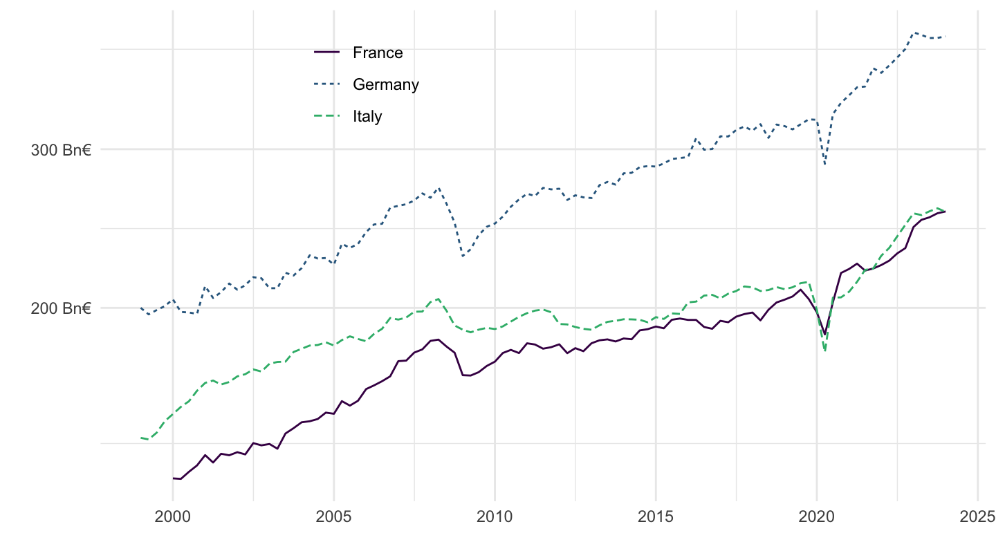
Tables
France
Code
nasq_10_nf_tr %>%
  filter(geo == "FR",
         time == "2019Q1",
         s_adj == "NSA",
         direct == "PAID",
         unit == "CP_MNAC") %>%
  left_join(namq_10_gdp_B1GQ_NSA_CPMNAC, by = c("geo", "time")) %>%
  mutate(values = round(100*values/B1GQ_NSA_CPMNAC, 1) %>% paste0("%")) %>%
  left_join(na_item, by = "na_item") %>%
  select(na_item, Na_item, sector, values) %>%
  spread(sector, values) %>%
  {if (is_html_output()) datatable(., filter = 'top', rownames = F) else .}
Germany
Code
nasq_10_nf_tr %>%
  filter(geo == "DE",
         time == "2019Q1",
         s_adj == "NSA",
         direct == "PAID",
         unit == "CP_MNAC") %>%
  left_join(namq_10_gdp_B1GQ_NSA_CPMNAC, by = c("geo", "time")) %>%
  mutate(values = round(100*values/B1GQ_NSA_CPMNAC, 1) %>% paste0("%")) %>%
  left_join(na_item, by = "na_item") %>%
  select(na_item, Na_item, sector, values) %>%
  spread(sector, values) %>%
  {if (is_html_output()) datatable(., filter = 'top', rownames = F) else .}
Italy
Code
nasq_10_nf_tr %>%
  filter(geo == "IT",
         time == "2019Q1",
         s_adj == "NSA",
         direct == "PAID",
         unit == "CP_MNAC") %>%
  left_join(namq_10_gdp_B1GQ_NSA_CPMNAC, by = c("geo", "time")) %>%
  mutate(values = round(100*values/B1GQ_NSA_CPMNAC, 1) %>% paste0("%")) %>%
  left_join(na_item, by = "na_item") %>%
  select(na_item, Na_item, sector, values) %>%
  spread(sector, values) %>%
  {if (is_html_output()) datatable(., filter = 'top', rownames = F) else .}
B8G
France
Code
nasq_10_nf_tr %>%
  filter(geo == "FR",
         time == "2019Q1",
         s_adj == "NSA",
         direct == "PAID",
         unit == "CP_MNAC") %>%
  left_join(namq_10_gdp_B1GQ_NSA_CPMNAC, by = c("geo", "time")) %>%
  mutate(values = round(100*values/B1GQ_NSA_CPMNAC, 1) %>% paste0("%")) %>%
  left_join(na_item, by = "na_item") %>%
  select(na_item, Na_item, sector, values) %>%
  spread(sector, values) %>%
  {if (is_html_output()) datatable(., filter = 'top', rownames = F) else .}
France
Code
nasq_10_nf_tr %>%
  filter(geo == "FR",
         na_item == "B8G",
         s_adj == "SCA",
         #direct == "PAID",
         unit == "CP_MNAC") %>%
  select(geo, time, values, sector, direct) %>%
  left_join(namq_10_gdp_B1GQ_NSA_CPMNAC, by = c("geo", "time")) %>%
  mutate(values = values/B1GQ_NSA_CPMNAC) %>%
  quarter_to_date %>%
  left_join(sector, by = "sector") %>%
  ggplot + theme_minimal() + xlab("") + ylab("") +
  geom_line(aes(x = date, y = values, color = Sector, linetype = direct)) +
  scale_x_date(breaks = as.Date(paste0(seq(1940, 2100, 5), "-01-01")),
               labels = date_format("%Y")) +
  theme(legend.position = c(0.4, 0.7),
        legend.title = element_blank()) +
  scale_y_continuous(breaks = 0.01*seq(0, 100, 1),
                labels = percent_format(a = 1))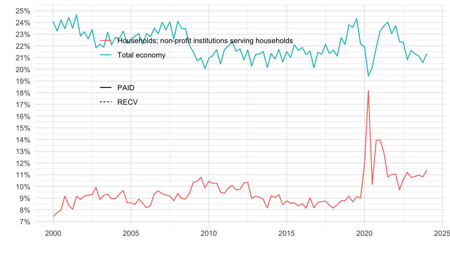
Germany
Code
nasq_10_nf_tr %>%
  filter(geo == "DE",
         na_item == "B8G",
         s_adj == "SCA",
         direct == "PAID",
         unit == "CP_MNAC") %>%
  select(geo, time, values, sector) %>%
  left_join(namq_10_gdp_B1GQ_NSA_CPMNAC, by = c("geo", "time")) %>%
  mutate(values = values/B1GQ_NSA_CPMNAC) %>%
  quarter_to_date %>%
  left_join(sector, by = "sector") %>%
  ggplot + theme_minimal() + xlab("") + ylab("") +
  geom_line(aes(x = date, y = values, color = Sector)) +
  scale_color_manual(values = viridis(4)[1:3]) +
  scale_x_date(breaks = as.Date(paste0(seq(1940, 2100, 5), "-01-01")),
               labels = date_format("%Y")) +
  theme(legend.position = c(0.3, 0.85),
        legend.title = element_blank()) +
  scale_y_continuous(breaks = 0.01*seq(0, 100, 1),
                labels = percent_format(a = 1))
France, Germany, Italy
B8G - Saving, Gross
Code
nasq_10_nf_tr %>%
  filter(geo %in% c("FR", "DE", "IT", "ES", "NL"),
         # B2A3G: Operating surplus and mixed income, gross
         na_item == "B8G",
         # SCA: Seasonally and calendar adjusted data
         s_adj == "SCA",
         # PAID: Paid
         direct == "PAID",
         # CP_MNAC: Current prices, million units of national currency
         unit == "CP_MNAC",
         # S1: Total economy
         sector == "S1") %>%
  quarter_to_date %>%
  left_join(geo, by = "geo") %>%
  mutate(values = values/1000) %>%
  left_join(colors, by = c( "Geo" = "country")) %>%
  ggplot + geom_line(aes(x = date, y = values, color = color)) +
  scale_color_identity() + theme_minimal()  + xlab("") + ylab("") + add_4flags +
  scale_x_date(breaks = as.Date(paste0(seq(1940, 2100, 5), "-01-01")),
               labels = date_format("%Y")) +
  theme(legend.position = c(0.3, 0.85),
        legend.title = element_blank()) +
  scale_y_log10(breaks = c(c(1, 2, 3, 5, 8, 10),
                           10*c(1, 2, 3, 5, 8, 10),
                           100*c(1, 2, 3, 5, 8, 10)),
                labels = dollar_format(suffix = " Bn€", prefix = "", accuracy = 1))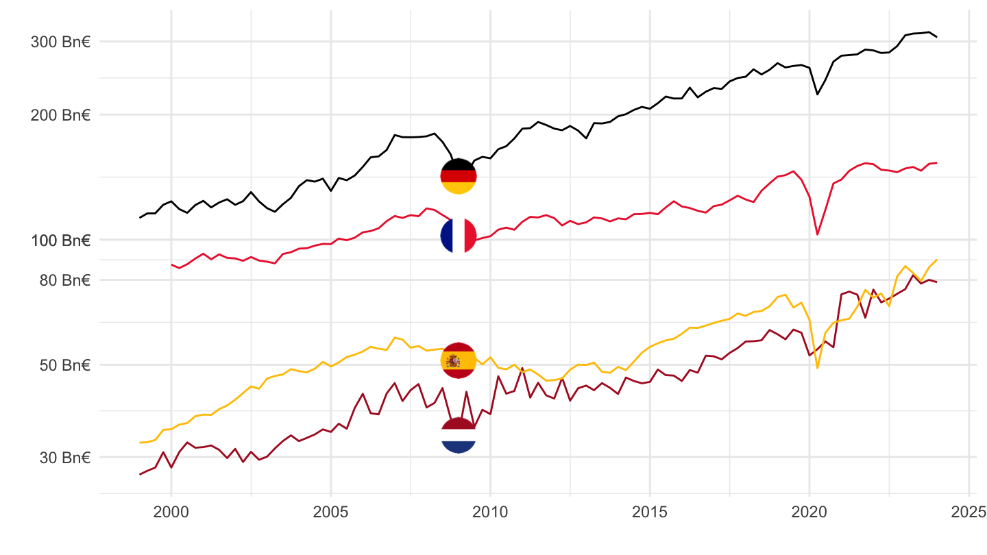
B6G_R_HAB - GDI of households in real terms per capita
1999-
Value
Code
nasq_10_nf_tr %>%
  filter(geo %in% c("FR", "DE", "IT", "ES", "NL"),
         # B2A3G: Operating surplus and mixed income, gross
         na_item == "B6G_R_HAB",
         # SCA: Seasonally and calendar adjusted data
         s_adj == "SCA",
         # PAID: Paid
         direct == "PAID",
         # CP_MNAC: Current prices, million units of national currency
         unit == "CP_MNAC") %>%
  quarter_to_date %>%
  filter(date >= as.Date("1999-01-01")) %>%
  left_join(geo, by = "geo") %>%
  left_join(colors, by = c( "Geo" = "country")) %>%
  ggplot + geom_line(aes(x = date, y = values, color = color, linetype = direct)) +
  scale_color_identity() + theme_minimal()  + xlab("") + ylab("") + add_5flags +
  scale_x_date(breaks = as.Date(paste0(seq(1940, 2100, 2), "-01-01")),
               labels = date_format("%Y")) +
  theme(legend.position = c(0.3, 0.85),
        legend.title = element_blank())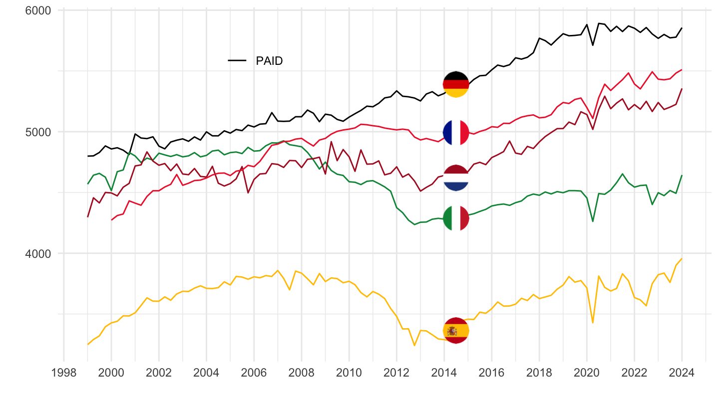
Index = 1999
These
Code
nasq_10_nf_tr %>%
  filter(geo %in% c("FR", "DE", "IT", "ES", "EA"),
         # B2A3G: Operating surplus and mixed income, gross
         na_item == "B6G_R_HAB",
         # SCA: Seasonally and calendar adjusted data
         s_adj == "SCA",
         # PAID: Paid
         direct == "PAID",
         # CP_MNAC: Current prices, million units of national currency
         unit == "CP_MNAC") %>%
  quarter_to_date %>%
  filter(date >= as.Date("1999-01-01")) %>%
  left_join(geo, by = "geo") %>%
  group_by(geo) %>%
  arrange(date) %>%
  mutate(values = 100*values/values[1]) %>%
  left_join(colors, by = c( "Geo" = "country")) %>%
  ggplot + geom_line(aes(x = date, y = values, color = color)) +
  scale_color_identity() + theme_minimal()  + xlab("") + ylab("GDI of households in real terms per capita") + add_5flags +
  scale_x_date(breaks = as.Date(paste0(seq(1999, 2100, 2), "-01-01")),
               labels = date_format("%Y")) +
  theme(legend.position = c(0.3, 0.85),
        legend.title = element_blank()) +
  scale_y_log10(breaks = seq(10, 200, 2)) +
  geom_label_repel(data = . %>% filter(date == max(date)), aes(x = date, y = values, label = round(values, 1), color = color))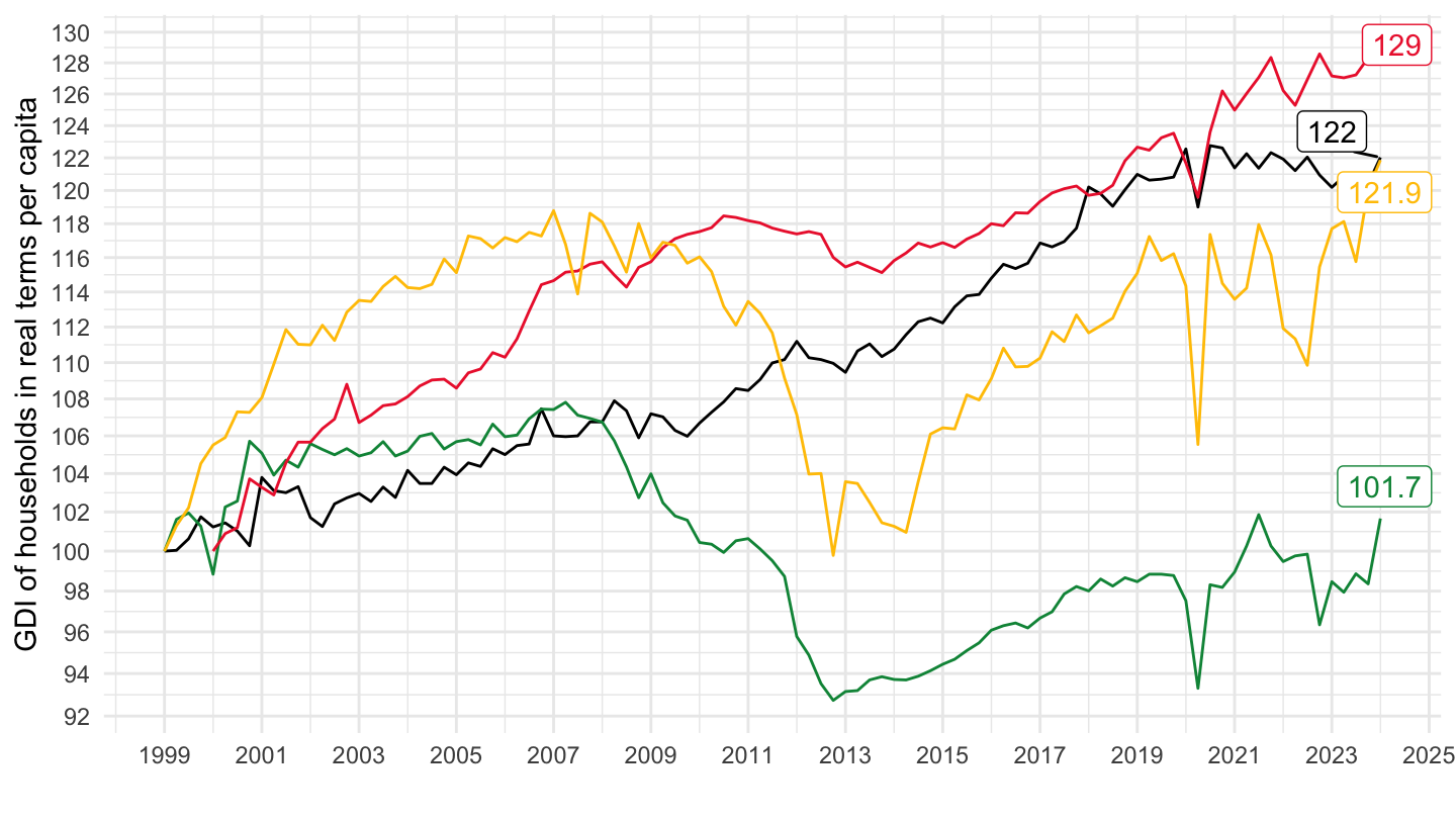
Index = 1999
These
Code
nasq_10_nf_tr %>%
  filter(geo %in% c("FR", "DE", "IT", "ES", "NL"),
         # B2A3G: Operating surplus and mixed income, gross
         na_item == "B6G_R_HAB",
         # SCA: Seasonally and calendar adjusted data
         s_adj == "SCA",
         # PAID: Paid
         direct == "PAID",
         # CP_MNAC: Current prices, million units of national currency
         unit == "CP_MNAC") %>%
  quarter_to_date %>%
  filter(date >= as.Date("1999-01-01")) %>%
  left_join(geo, by = "geo") %>%
  group_by(geo) %>%
  arrange(date) %>%
  mutate(values = 100*values/values[1]) %>%
  left_join(colors, by = c( "Geo" = "country")) %>%
  ggplot + geom_line(aes(x = date, y = values, color = color)) +
  scale_color_identity() + theme_minimal()  + xlab("") + ylab("GDI of households in real terms per capita") + add_5flags +
  scale_x_date(breaks = as.Date(paste0(seq(1999, 2100, 2), "-01-01")),
               labels = date_format("%Y")) +
  theme(legend.position = c(0.3, 0.85),
        legend.title = element_blank()) +
  scale_y_log10(breaks = seq(10, 200, 2)) +
  geom_label_repel(data = . %>% filter(date == max(date)), aes(x = date, y = values, label = round(values, 1), color = color))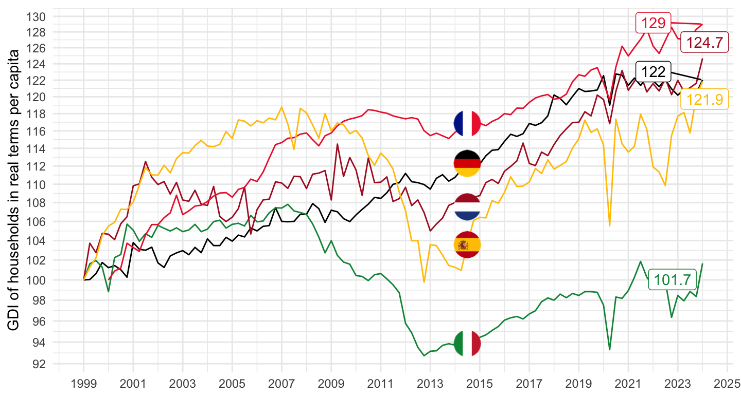
All
Code
nasq_10_nf_tr %>%
  filter(na_item == "B6G_R_HAB",
         # SCA: Seasonally and calendar adjusted data
         s_adj == "SCA",
         # PAID: Paid
         direct == "PAID",
         # CP_MNAC: Current prices, million units of national currency
         unit == "CP_MNAC") %>%
  quarter_to_date %>%
  filter(date >= as.Date("1999-01-01")) %>%
  left_join(geo, by = "geo") %>%
  group_by(geo) %>%
  arrange(date) %>%
  mutate(values = 100*values/values[1]) %>%
  left_join(colors, by = c( "Geo" = "country")) %>%
  ggplot + geom_line(aes(x = date, y = values, color = color)) +
  scale_color_identity() + theme_minimal()  + xlab("") + ylab("GDI of households in real terms per capita") +
  scale_x_date(breaks = as.Date(paste0(seq(1999, 2100, 2), "-01-01")),
               labels = date_format("%Y")) +
  theme(legend.position = c(0.3, 0.85),
        legend.title = element_blank()) +
  scale_y_log10(breaks = seq(10, 200, 2)) +
  geom_label_repel(data = . %>% filter(date == max(date)), aes(x = date, y = values, label = paste0(Geo, ": ", round(values, 1)), color = color))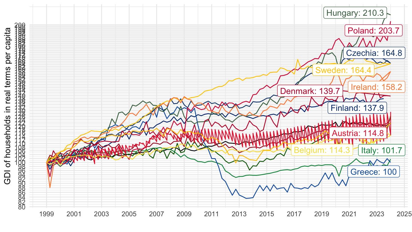
2017-
Code
nasq_10_nf_tr %>%
  filter(geo %in% c("FR", "DE", "IT", "ES", "NL"),
         # B2A3G: Operating surplus and mixed income, gross
         na_item == "B6G_R_HAB",
         # SCA: Seasonally and calendar adjusted data
         s_adj == "SCA",
         # PAID: Paid
         direct == "PAID",
         # CP_MNAC: Current prices, million units of national currency
         unit == "CP_MNAC") %>%
  quarter_to_date %>%
  filter(date >= as.Date("2017-01-01")) %>%
  left_join(geo, by = "geo") %>%
  group_by(geo) %>%
  arrange(date) %>%
  mutate(values = 100*values/values[1]) %>%
  left_join(colors, by = c( "Geo" = "country")) %>%
  ggplot + geom_line(aes(x = date, y = values, color = color)) +
  scale_color_identity() + theme_minimal()  + xlab("") + ylab("B6G - Disposable income, Gross") + add_5flags +
  scale_x_date(breaks = as.Date(paste0(seq(1940, 2100, 1), "-01-01")),
               labels = date_format("%Y")) +
  theme(legend.position = c(0.3, 0.85),
        legend.title = element_blank()) +
  scale_y_log10(breaks = seq(10, 200, 2))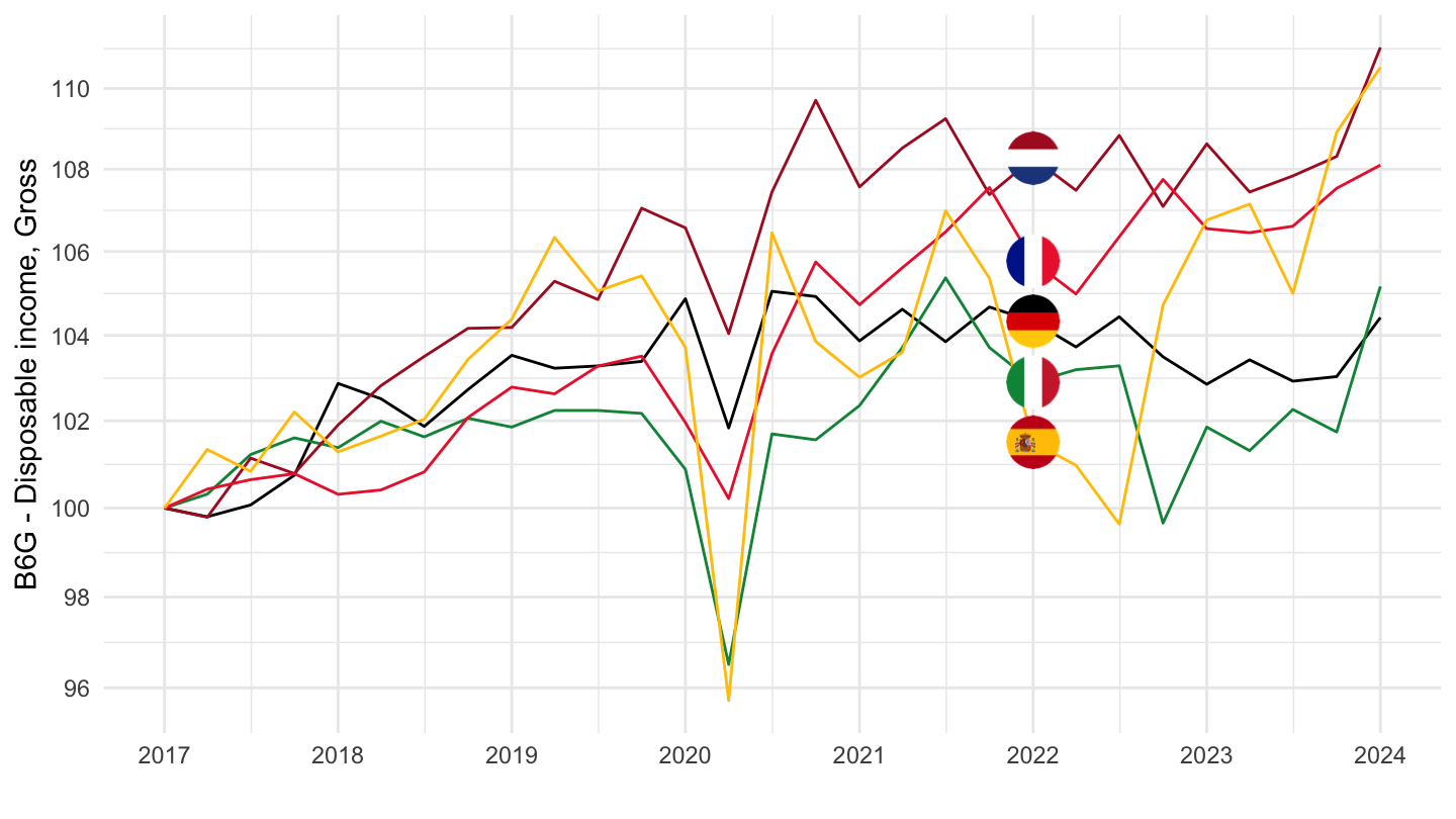
Implicit price index in it
B6G/POP/B6G_R_HAB
Code
nasq_10_nf_tr %>%
  filter(geo %in% c("FR", "DE", "IT", "ES", "NL"),
         # B2A3G: Operating surplus and mixed income, gross
         na_item %in% c("B6G_R_HAB", "B6G"),
         sector == "S14_S15",
         # SCA: Seasonally and calendar adjusted data
         s_adj == "SCA",
         # PAID: Paid
         direct == "PAID",
         # CP_MNAC: Current prices, million units of national currency
         unit == "CP_MNAC") %>%
  select(time, geo, na_item, values) %>%
  spread(na_item, values) %>%
  left_join(POP, by = c("geo", "time")) %>%
  transmute(time, geo, values = B6G/NSA/B6G_R_HAB) %>%
  quarter_to_date %>%
  filter(date >= as.Date("1999-01-01")) %>%
  left_join(geo, by = "geo") %>%
  group_by(geo) %>%
  arrange(date) %>%
  mutate(values = 100*values/values[1]) %>%
  left_join(colors, by = c( "Geo" = "country")) %>%
  ggplot + geom_line(aes(x = date, y = values, color = color)) +
  scale_color_identity() + theme_minimal()  + xlab("") + ylab("Implicit price index") + add_5flags +
  scale_x_date(breaks = as.Date(paste0(seq(1999, 2100, 2), "-01-01")),
               labels = date_format("%Y")) +
  theme(legend.position = c(0.3, 0.85),
        legend.title = element_blank()) +
  scale_y_log10(breaks = seq(10, 200, 2)) +
  geom_label_repel(data = . %>% filter(date == max(date)), aes(x = date, y = values, label = paste0(date, " : ", round(values, 1)), color = color))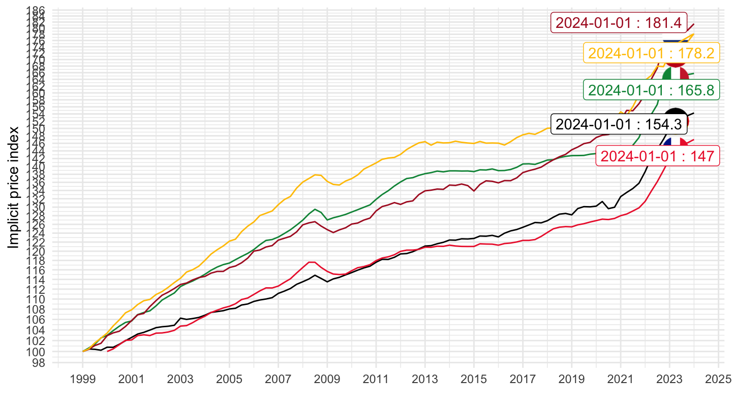
B6G - Disposable income, Gross
All
Code
nasq_10_nf_tr %>%
  filter(geo %in% c("FR", "DE", "IT", "ES", "NL"),
         # B2A3G: Operating surplus and mixed income, gross
         na_item == "B6G",
         # SCA: Seasonally and calendar adjusted data
         s_adj == "SCA",
         # PAID: Paid
         direct == "PAID",
         # CP_MNAC: Current prices, million units of national currency
         unit == "CP_MNAC",
         # S1: Total economy
         sector == "S1") %>%
  quarter_to_date %>%
  left_join(geo, by = "geo") %>%
  mutate(values = values/1000) %>%
  left_join(colors, by = c( "Geo" = "country")) %>%
  ggplot + geom_line(aes(x = date, y = values, color = color)) +
  scale_color_identity() + theme_minimal()  + xlab("") + ylab("") + add_4flags +
  scale_x_date(breaks = as.Date(paste0(seq(1940, 2100, 5), "-01-01")),
               labels = date_format("%Y")) +
  theme(legend.position = c(0.3, 0.85),
        legend.title = element_blank()) +
  scale_y_log10(breaks = c(c(1, 2, 3, 5, 8, 10),
                           10*c(1, 2, 3, 5, 8, 10),
                           100*c(1, 2, 3, 5, 8, 10)),
                labels = dollar_format(suffix = " Bn€", prefix = "", accuracy = 1))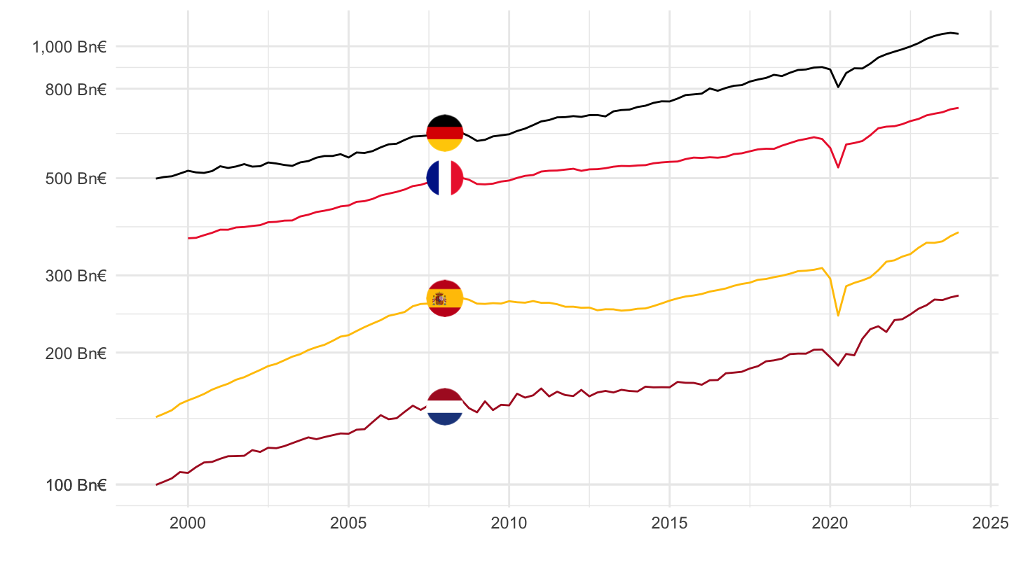
1996-
Code
nasq_10_nf_tr %>%
  filter(geo %in% c("FR", "DE", "IT", "ES", "NL"),
         # B2A3G: Operating surplus and mixed income, gross
         na_item == "B6G",
         # SCA: Seasonally and calendar adjusted data
         s_adj == "SCA",
         # PAID: Paid
         direct == "PAID",
         # CP_MNAC: Current prices, million units of national currency
         unit == "CP_MNAC",
         # S1: Total economy
         sector == "S1") %>%
  quarter_to_date %>%
  filter(date >= as.Date("1996-01-01")) %>%
  left_join(geo, by = "geo") %>%
  group_by(geo) %>%
  arrange(date) %>%
  mutate(values = 100*values/values[1]) %>%
  left_join(colors, by = c( "Geo" = "country")) %>%
  ggplot + geom_line(aes(x = date, y = values, color = color)) +
  scale_color_identity() + theme_minimal()  + xlab("") + ylab("B6G - Disposable income, Gross") + add_4flags +
  scale_x_date(breaks = as.Date(paste0(seq(1995, 2100, 2), "-01-01")),
               labels = date_format("%Y")) +
  theme(legend.position = c(0.3, 0.85),
        legend.title = element_blank()) +
  scale_y_log10(breaks = seq(10, 1000, 5)) +
  geom_label_repel(data = . %>% filter(date == max(date)), aes(x = date, y = values, label = round(values, 1), color = color))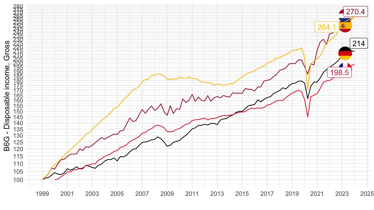
1999-
These
Code
nasq_10_nf_tr %>%
  filter(geo %in% c("FR", "DE", "IT", "ES", "NL"),
         # B2A3G: Operating surplus and mixed income, gross
         na_item == "B6G",
         # SCA: Seasonally and calendar adjusted data
         s_adj == "SCA",
         # PAID: Paid
         direct == "PAID",
         # CP_MNAC: Current prices, million units of national currency
         unit == "CP_MNAC",
         # S1: Total economy
         sector == "S1") %>%
  quarter_to_date %>%
  filter(date >= as.Date("1999-01-01")) %>%
  left_join(geo, by = "geo") %>%
  group_by(geo) %>%
  arrange(date) %>%
  mutate(values = 100*values/values[1]) %>%
  left_join(colors, by = c( "Geo" = "country")) %>%
  ggplot + geom_line(aes(x = date, y = values, color = color)) +
  scale_color_identity() + theme_minimal()  + xlab("") + ylab("B6G - Disposable income, Gross") + add_4flags +
  scale_x_date(breaks = as.Date(paste0(seq(1999, 2100, 2), "-01-01")),
               labels = date_format("%Y")) +
  theme(legend.position = c(0.3, 0.85),
        legend.title = element_blank()) +
  scale_y_log10(breaks = seq(10, 1000, 5)) +
  geom_label_repel(data = . %>% filter(date == max(date)), aes(x = date, y = values, label = paste0(Geo, ": ", round(values, 1)), color = color))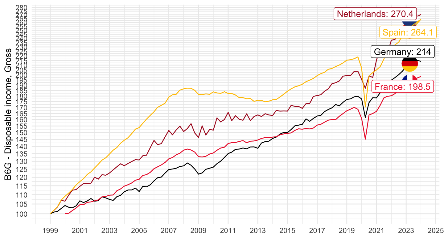
Population
Code
nasq_10_nf_tr %>%
  filter(geo %in% c("FR", "DE", "IT", "ES", "NL"),
         # B2A3G: Operating surplus and mixed income, gross
         na_item == "B6G",
         # SCA: Seasonally and calendar adjusted data
         s_adj == "NSA",
         # PAID: Paid
         direct == "PAID",
         # CP_MNAC: Current prices, million units of national currency
         unit == "CP_MNAC",
         # S1: Total economy
         sector == "S1") %>%
  left_join(POP, by = c("geo", "time")) %>%
  quarter_to_date %>%
  filter(date >= as.Date("1999-01-01")) %>%
  left_join(geo, by = "geo") %>%
  group_by(geo) %>%
  arrange(date) %>%
  mutate(values = values/NSA) %>%
  mutate(values = 100*values/values[1]) %>%
  left_join(colors, by = c( "Geo" = "country")) %>%
  ggplot + geom_line(aes(x = date, y = values, color = color)) +
  scale_color_identity() + theme_minimal()  + xlab("") + ylab("B6G - Disposable income, Gross/Population") + add_4flags +
  scale_x_date(breaks = as.Date(paste0(seq(1999, 2100, 2), "-01-01")),
               labels = date_format("%Y")) +
  theme(legend.position = c(0.3, 0.85),
        legend.title = element_blank()) +
  scale_y_log10(breaks = seq(10, 1000, 5)) +
  geom_label_repel(data = . %>% filter(date == max(date)), aes(x = date, y = values, label = paste0(Geo, ": ", round(values, 1)), color = color))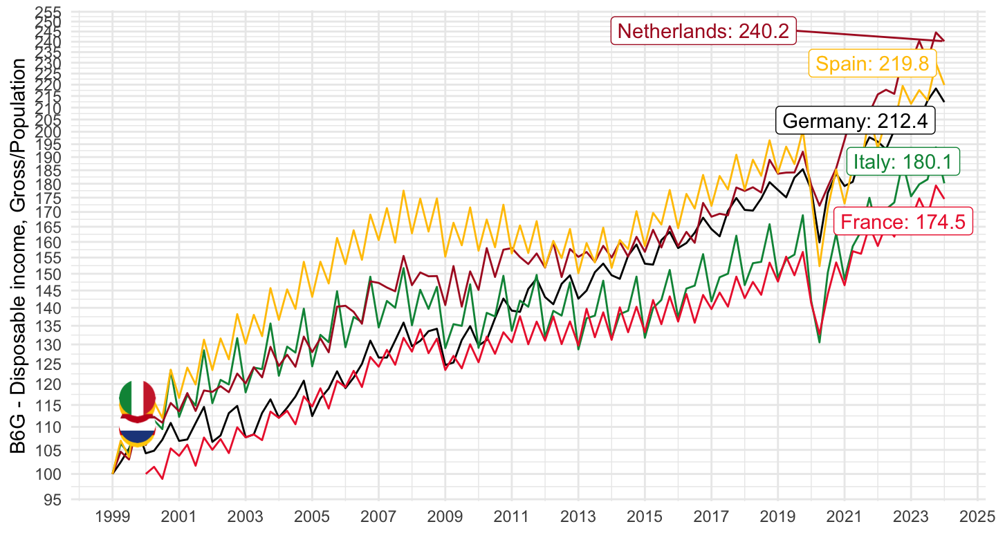
All
Code
nasq_10_nf_tr %>%
  filter(na_item == "B6G",
         geo != "RO",
         # SCA: Seasonally and calendar adjusted data
         s_adj == "SCA",
         # PAID: Paid
         direct == "PAID",
         # CP_MNAC: Current prices, million units of national currency
         unit == "CP_MNAC",
         # S1: Total economy
         sector == "S1") %>%
  quarter_to_date %>%
  filter(date >= as.Date("1999-01-01")) %>%
  left_join(geo, by = "geo") %>%
  group_by(geo) %>%
  arrange(date) %>%
  mutate(values = 100*values/values[1]) %>%
  left_join(colors, by = c( "Geo" = "country")) %>%
  ggplot + geom_line(aes(x = date, y = values, color = color)) +
  scale_color_identity() + theme_minimal()  + xlab("") + ylab("B6G - Disposable income, Gross") + add_4flags +
  scale_x_date(breaks = as.Date(paste0(seq(1999, 2100, 2), "-01-01")),
               labels = date_format("%Y")) +
  theme(legend.position = c(0.3, 0.85),
        legend.title = element_blank()) +
  scale_y_log10(breaks = seq(10, 1000, 5)) +
  geom_label_repel(data = . %>% filter(date == max(date)), aes(x = date, y = values, label = paste0(Geo, ": ", round(values, 1)), color = color))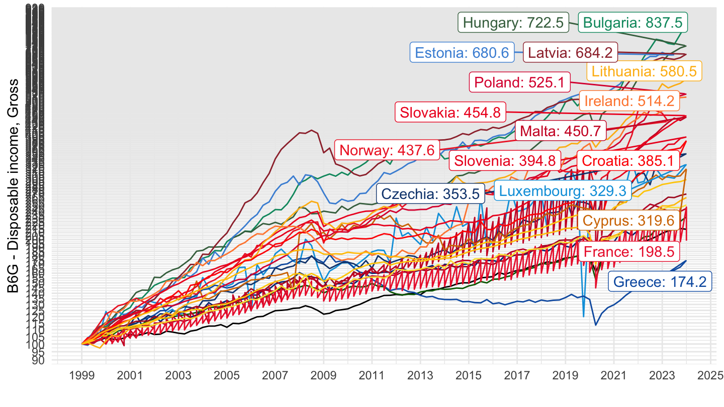
2001-
Code
nasq_10_nf_tr %>%
  filter(geo %in% c("FR", "DE", "IT", "ES", "EA20"),
         # B2A3G: Operating surplus and mixed income, gross
         na_item == "B6G",
         # SCA: Seasonally and calendar adjusted data
         s_adj == "SCA",
         # PAID: Paid
         direct == "PAID",
         # CP_MNAC: Current prices, million units of national currency
         unit == "CP_MNAC",
         # S1: Total economy
         sector == "S1") %>%
  left_join(POP, by = c("geo", "time")) %>%
  quarter_to_date %>%
  filter(date >= as.Date("2001-01-01")) %>%
  left_join(geo, by = "geo") %>%
  group_by(geo) %>%
  arrange(date) %>%
  mutate(values = values/NSA) %>%
  mutate(values = 100*values/values[1]) %>%
  left_join(colors, by = c( "Geo" = "country")) %>%
  ggplot + geom_line(aes(x = date, y = values, color = color)) +
  scale_color_identity() + theme_minimal()  + xlab("") + ylab("B6G - Disposable income, Gross/Population") + add_4flags +
  scale_x_date(breaks = as.Date(paste0(seq(1999, 2100, 2), "-01-01")),
               labels = date_format("%Y")) +
  theme(legend.position = c(0.3, 0.85),
        legend.title = element_blank()) +
  scale_y_log10(breaks = seq(10, 1000, 5)) +
  geom_label_repel(data = . %>% filter(date == max(date)), aes(x = date, y = values, label = paste0(Geo, ": ", round(values, 1)), color = color))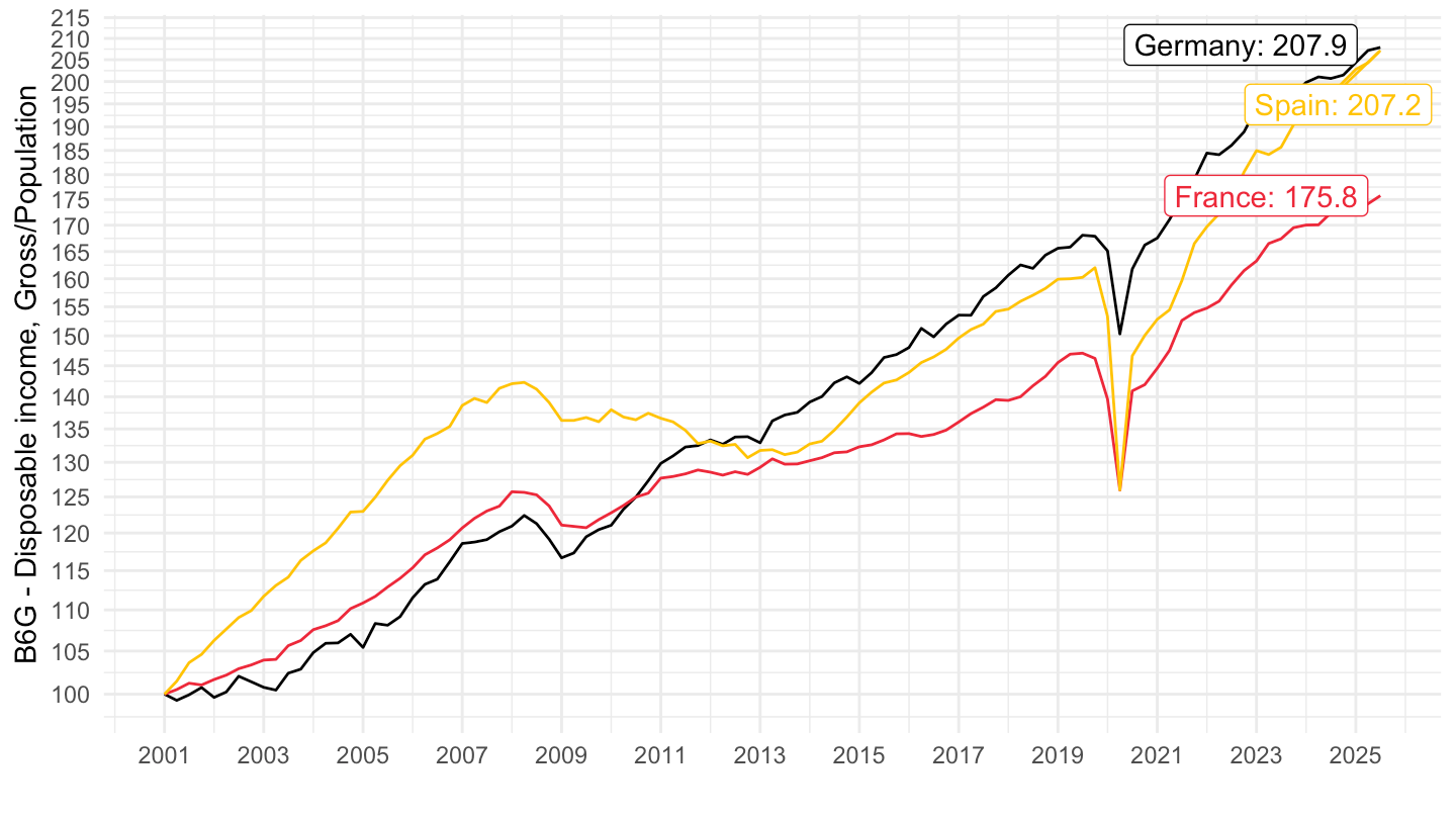
2017-
Nominal
Code
nasq_10_nf_tr %>%
  filter(geo %in% c("FR", "DE", "IT", "ES", "EA20"),
         # B2A3G: Operating surplus and mixed income, gross
         na_item == "B6G",
         # SCA: Seasonally and calendar adjusted data
         s_adj == "SCA",
         # PAID: Paid
         direct == "PAID",
         # CP_MNAC: Current prices, million units of national currency
         unit == "CP_MNAC",
         # S1: Total economy
         sector == "S1") %>%
  quarter_to_date %>%
  filter(date >= as.Date("2017-01-01")) %>%
  left_join(geo, by = "geo") %>%
  group_by(geo) %>%
  arrange(date) %>%
  mutate(values = 100*values/values[1]) %>%
  left_join(colors, by = c( "Geo" = "country")) %>%
  ggplot + geom_line(aes(x = date, y = values, color = color)) +
  scale_color_identity() + theme_minimal()  + xlab("") + ylab("B6G - Disposable income, Gross") + add_3flags +
  scale_x_date(breaks = as.Date(paste0(seq(1940, 2100, 1), "-01-01")),
               labels = date_format("%Y")) +
  theme(legend.position = c(0.3, 0.85),
        legend.title = element_blank()) +
  scale_y_log10(breaks = seq(10, 200, 5)) +
  geom_label_repel(data = . %>% filter(date == max(date)), aes(x = date, y = values, label = paste0(Geo, ": ", round(values, 1)), color = color))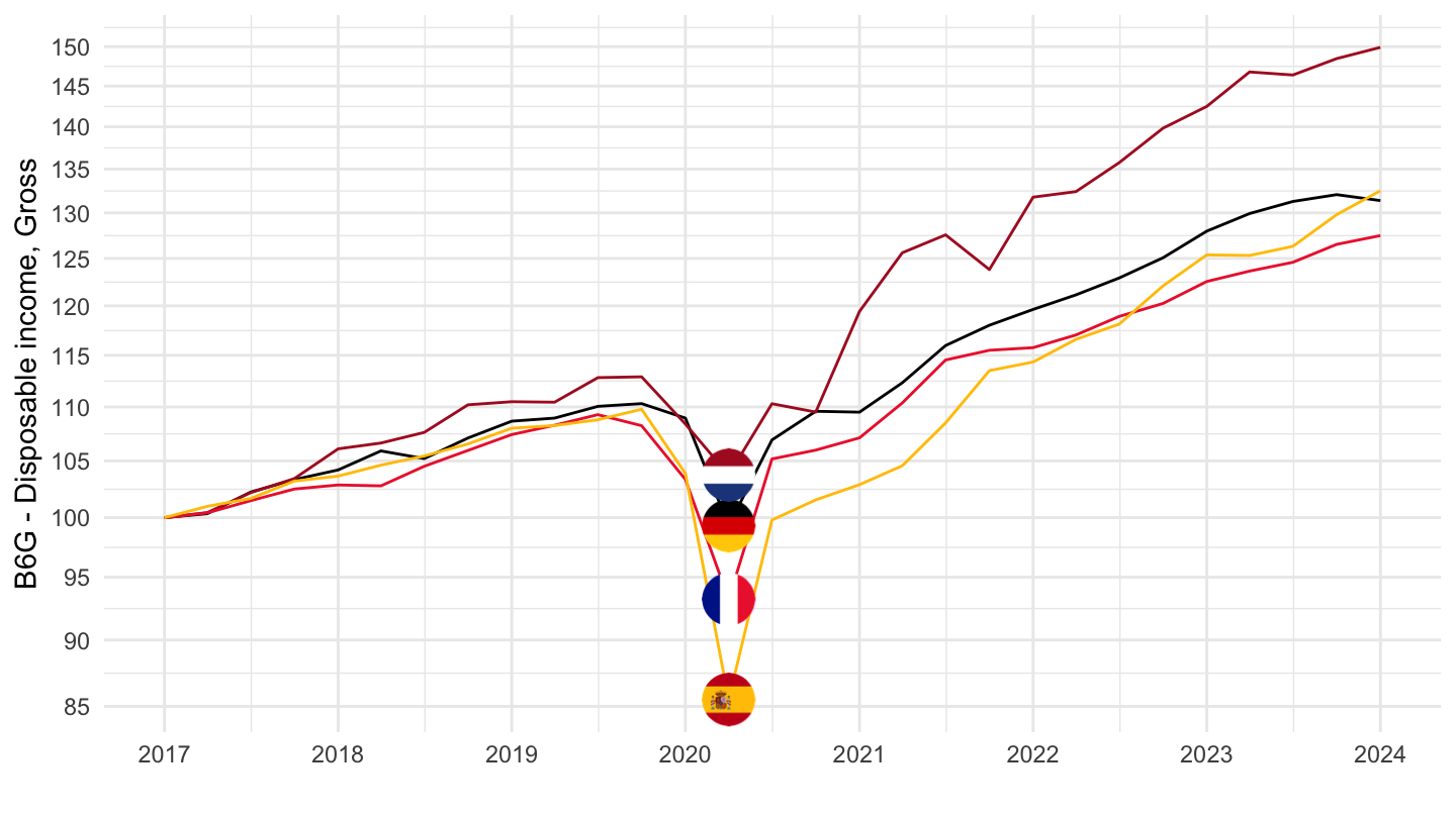
Nominal/population
Code
nasq_10_nf_tr %>%
  filter(geo %in% c("FR", "DE", "IT", "ES", "EA20"),
         # B2A3G: Operating surplus and mixed income, gross
         na_item == "B6G",
         # SCA: Seasonally and calendar adjusted data
         s_adj == "SCA",
         # PAID: Paid
         direct == "PAID",
         # CP_MNAC: Current prices, million units of national currency
         unit == "CP_MNAC",
         # S1: Total economy
         sector == "S1") %>%
  left_join(POP, by = c("geo", "time")) %>%
  quarter_to_date %>%
  filter(date >= as.Date("2017-01-01")) %>%
  left_join(geo, by = "geo") %>%
  group_by(geo) %>%
  arrange(date) %>%
  mutate(values = values / NSA) %>%
  mutate(values = 100*values/values[1]) %>%
  left_join(colors, by = c( "Geo" = "country")) %>%
  ggplot + geom_line(aes(x = date, y = values, color = color)) +
  scale_color_identity() + theme_minimal()  + xlab("") + ylab("B6G - Disposable income, Gross / Population") + add_3flags +
  scale_x_date(breaks = as.Date(paste0(seq(1940, 2100, 1), "-01-01")),
               labels = date_format("%Y")) +
  theme(legend.position = c(0.3, 0.85),
        legend.title = element_blank()) +
  scale_y_log10(breaks = seq(10, 200, 5)) +
  geom_label_repel(data = . %>% filter(date == max(date)), aes(x = date, y = values, label = paste0(Geo, ": ", round(values, 1)), color = color))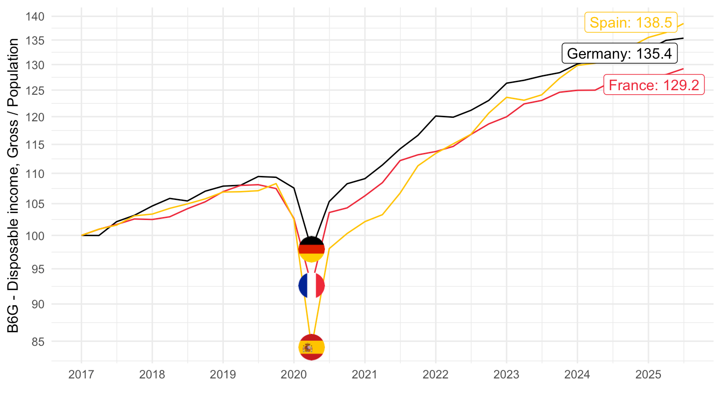
Households
Code
nasq_10_nf_tr %>%
  filter(geo %in% c("FR", "DE", "IT", "ES", "NL"),
         # B2A3G: Operating surplus and mixed income, gross
         na_item == "B6G",
         # SCA: Seasonally and calendar adjusted data
         s_adj == "SCA",
         # PAID: Paid
         direct == "PAID",
         # CP_MNAC: Current prices, million units of national currency
         unit == "CP_MNAC",
         # S1: Total economy
         sector == "S14_S15") %>%
  quarter_to_date %>%
  left_join(geo, by = "geo") %>%
  mutate(values = values/1000) %>%
  left_join(colors, by = c( "Geo" = "country")) %>%
  ggplot + geom_line(aes(x = date, y = values, color = color)) +
  scale_color_identity() + theme_minimal()  + xlab("") + ylab("") + add_5flags +
  scale_x_date(breaks = as.Date(paste0(seq(1940, 2100, 5), "-01-01")),
               labels = date_format("%Y")) +
  theme(legend.position = c(0.3, 0.85),
        legend.title = element_blank()) +
  scale_y_log10(breaks = c(c(1, 2, 3, 5, 8, 10),
                           10*c(1, 2, 3, 5, 8, 10),
                           100*c(1, 2, 3, 5, 8, 10)),
                labels = dollar_format(suffix = " Bn€", prefix = "", accuracy = 1))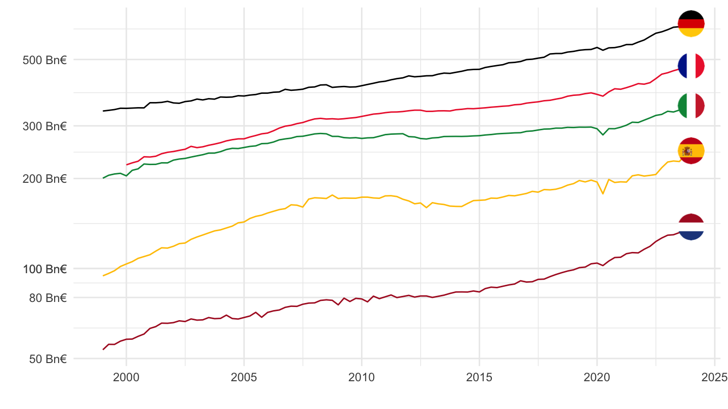
B2A3G - Operating surplus and mixed income, gross
All
Code
nasq_10_nf_tr %>%
  filter(geo %in% c("FR", "DE", "IT", "ES", "NL"),
         na_item == "B2A3G",
         s_adj == "SCA",
         direct == "PAID",
         unit == "CP_MNAC",
         sector == "S1") %>%
  quarter_to_date %>%
  left_join(geo, by = "geo") %>%
  mutate(values = values/1000) %>%
  left_join(colors, by = c( "Geo" = "country")) %>%
  ggplot + geom_line(aes(x = date, y = values, color = color)) +
  scale_color_identity() + theme_minimal()  + xlab("") + ylab("") + add_5flags +
  scale_x_date(breaks = as.Date(paste0(seq(1940, 2100, 5), "-01-01")),
               labels = date_format("%Y")) +
  theme(legend.position = c(0.3, 0.85),
        legend.title = element_blank()) +
  scale_y_log10(breaks = c(c(1, 2, 3, 5, 8, 10),
                           10*c(1, 2, 3, 5, 8, 10),
                           100*c(1, 2, 3, 5, 8, 10)),
                labels = dollar_format(suffix = " Bn€", prefix = "", accuracy = 1))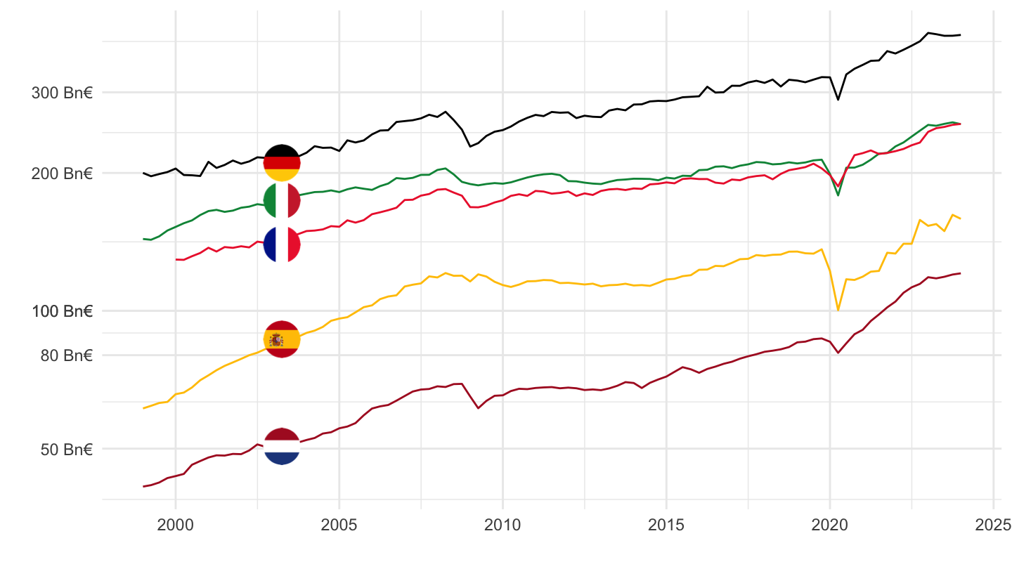
2000-
Code
nasq_10_nf_tr %>%
  filter(geo %in% c("FR", "DE", "IT", "ES", "NL"),
         na_item == "B2A3G",
         s_adj == "SCA",
         direct == "PAID",
         unit == "CP_MNAC",
         sector == "S1") %>%
  quarter_to_date %>%
  left_join(geo, by = "geo") %>%
  mutate(values = values/1000) %>%
  left_join(colors, by = c( "Geo" = "country")) %>%
  filter(date >= as.Date("2000-01-01")) %>%
  ggplot + geom_line(aes(x = date, y = values, color = color)) +
  scale_color_identity() + theme_minimal()  + xlab("") + ylab("") + add_5flags +
  scale_x_date(breaks = as.Date(paste0(seq(1940, 2100, 5), "-01-01")),
               labels = date_format("%Y")) +
  theme(legend.position = c(0.3, 0.85),
        legend.title = element_blank()) +
  scale_y_log10(breaks = c(c(1, 2, 3, 5, 8, 10),
                           10*c(1, 2, 3, 5, 8, 10),
                           100*c(1, 2, 3, 5, 8, 10)),
                labels = dollar_format(suffix = " Bn€", prefix = "", accuracy = 1))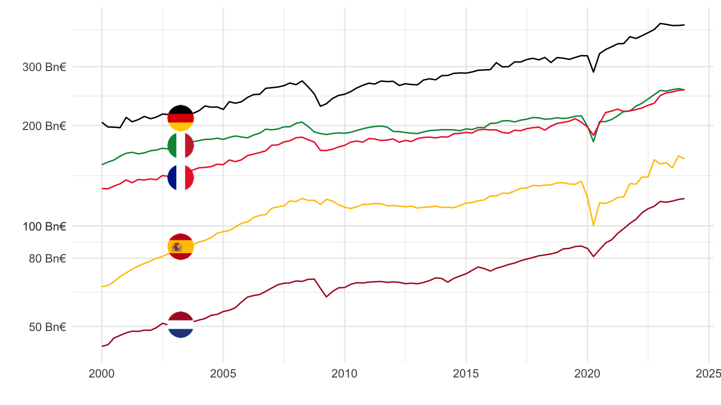
D4 - Property income
1999-
Code
nasq_10_nf_tr %>%
  filter(geo %in% c("FR", "DE", "IT", "ES", "NL"),
         # B2A3G: Operating surplus and mixed income, gross
         na_item == "D4",
         # SCA: Seasonally and calendar adjusted data
         s_adj == "SCA",
         # PAID: Paid
         direct == "PAID",
         # CP_MNAC: Current prices, million units of national currency
         unit == "CP_MNAC",
         # S1: Total economy
         sector == "S14_S15") %>%
  quarter_to_date %>%
  filter(date >= as.Date("1999-01-01")) %>%
  left_join(geo, by = "geo") %>%
  group_by(geo) %>%
  arrange(date) %>%
  mutate(values = 100*values/values[1]) %>%
  left_join(colors, by = c( "Geo" = "country")) %>%
  ggplot + geom_line(aes(x = date, y = values, color = color)) +
  scale_color_identity() + theme_minimal()  + xlab("") + ylab("Households, D4 - Property Income") + add_5flags +
  scale_x_date(breaks = as.Date(paste0(seq(1999, 2100, 5), "-01-01")),
               labels = date_format("%Y")) +
  theme(legend.position = c(0.3, 0.85),
        legend.title = element_blank()) +
  scale_y_log10(breaks = seq(20, 1000, 20))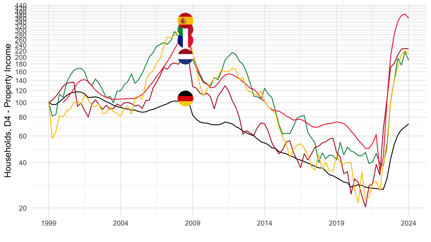
2017-
Code
nasq_10_nf_tr %>%
  filter(geo %in% c("FR", "DE", "IT", "ES", "NL"),
         # B2A3G: Operating surplus and mixed income, gross
         na_item == "D4",
         # SCA: Seasonally and calendar adjusted data
         s_adj == "SCA",
         # PAID: Paid
         direct == "PAID",
         # CP_MNAC: Current prices, million units of national currency
         unit == "CP_MNAC",
         # S1: Total economy
         sector == "S14_S15") %>%
  quarter_to_date %>%
  filter(date >= as.Date("2017-01-01")) %>%
  left_join(geo, by = "geo") %>%
  group_by(geo) %>%
  arrange(date) %>%
  mutate(values = 100*values/values[1]) %>%
  left_join(colors, by = c( "Geo" = "country")) %>%
  ggplot + geom_line(aes(x = date, y = values, color = color)) +
  scale_color_identity() + theme_minimal()  + xlab("") + ylab("Households, D4 - Property Income") + add_5flags +
  scale_x_date(breaks = as.Date(paste0(seq(1940, 2100, 1), "-01-01")),
               labels = date_format("%Y")) +
  theme(legend.position = c(0.3, 0.85),
        legend.title = element_blank()) +
  scale_y_log10(breaks = seq(20, 1000, 20))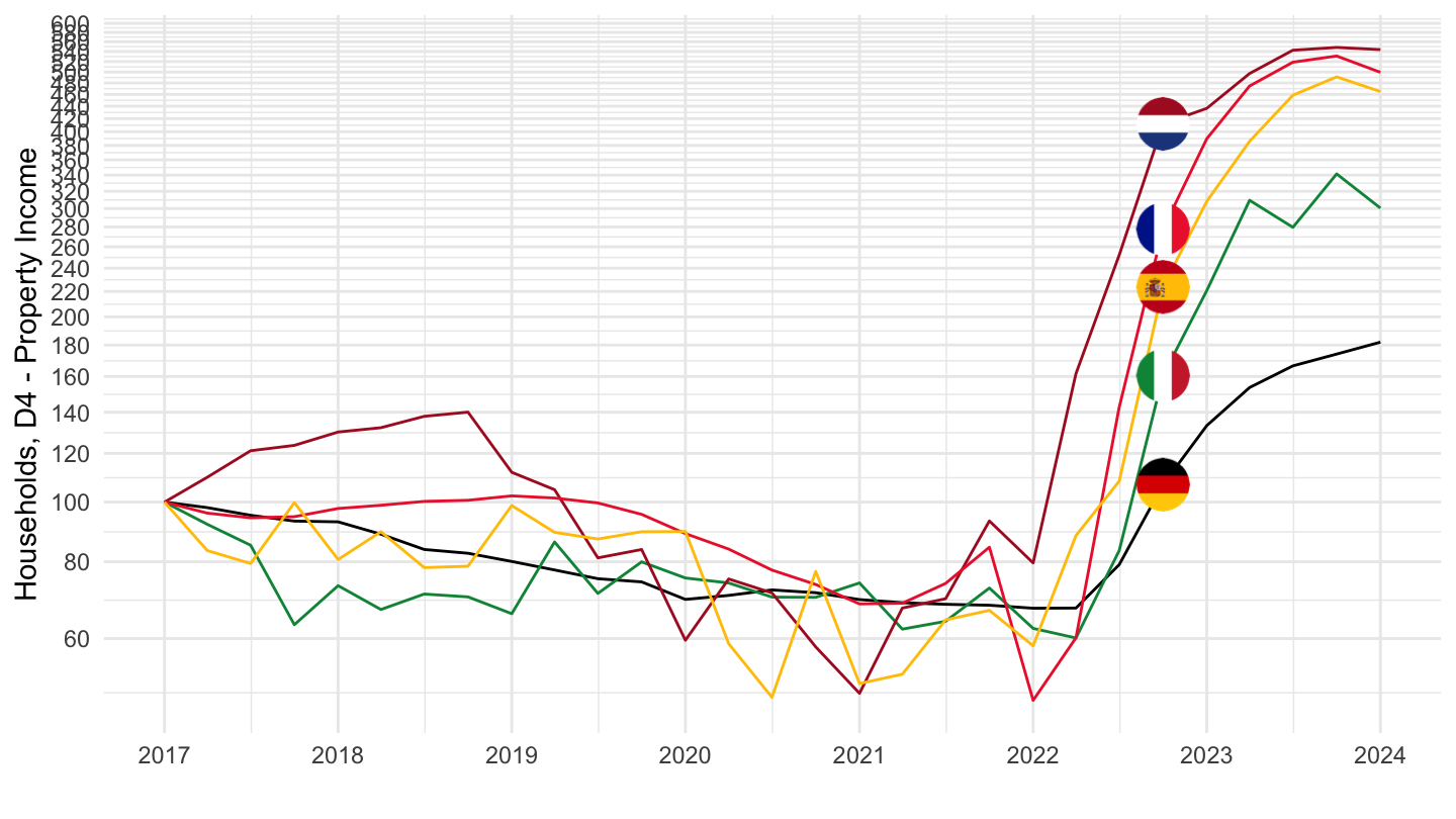
D41
1999-
Code
nasq_10_nf_tr %>%
  filter(geo %in% c("FR", "DE", "IT", "ES", "NL"),
         # B2A3G: Operating surplus and mixed income, gross
         na_item == "D41",
         # SCA: Seasonally and calendar adjusted data
         s_adj == "NSA",
         # PAID: Paid
         direct == "PAID",
         # CP_MNAC: Current prices, million units of national currency
         unit == "CP_MNAC",
         # S1: Total economy
         sector == "S14_S15") %>%
  quarter_to_date %>%
  filter(date >= as.Date("1999-01-01")) %>%
  left_join(geo, by = "geo") %>%
  group_by(geo) %>%
  arrange(date) %>%
  mutate(values = 100*values/values[1]) %>%
  left_join(colors, by = c( "Geo" = "country")) %>%
  ggplot + geom_line(aes(x = date, y = values, color = color)) +
  scale_color_identity() + theme_minimal()  + xlab("") + ylab("D41") + add_5flags +
  scale_x_date(breaks = as.Date(paste0(seq(1999, 2100, 5), "-01-01")),
               labels = date_format("%Y")) +
  theme(legend.position = c(0.3, 0.85),
        legend.title = element_blank()) +
  scale_y_log10(breaks = seq(20, 1000, 20))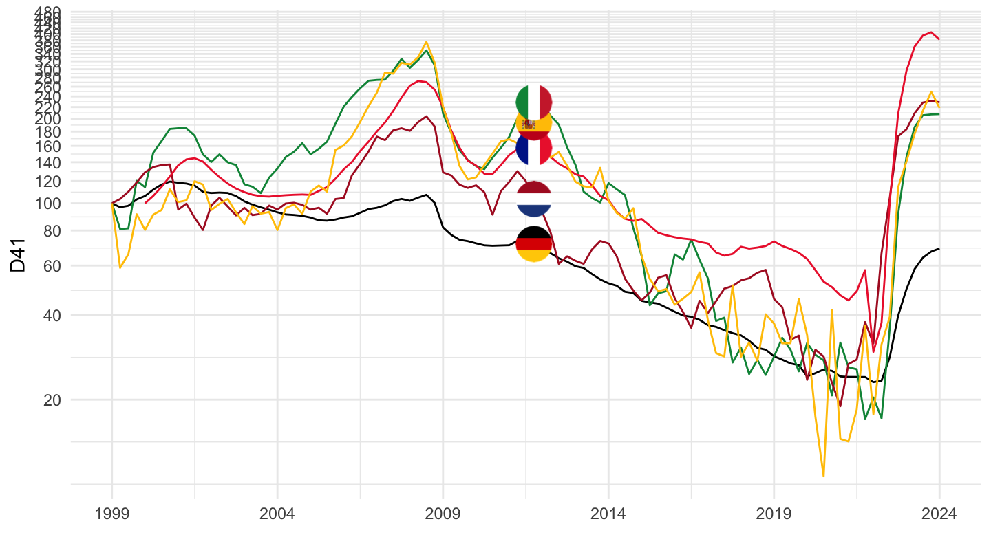
2017-
Code
nasq_10_nf_tr %>%
  filter(geo %in% c("FR", "DE", "IT", "ES", "NL"),
         # B2A3G: Operating surplus and mixed income, gross
         na_item == "D4",
         # SCA: Seasonally and calendar adjusted data
         s_adj == "NSA",
         # PAID: Paid
         direct == "PAID",
         # CP_MNAC: Current prices, million units of national currency
         unit == "CP_MNAC",
         # S1: Total economy
         sector == "S14_S15") %>%
  quarter_to_date %>%
  filter(date >= as.Date("2017-01-01")) %>%
  left_join(geo, by = "geo") %>%
  group_by(geo) %>%
  arrange(date) %>%
  mutate(values = 100*values/values[1]) %>%
  left_join(colors, by = c( "Geo" = "country")) %>%
  ggplot + geom_line(aes(x = date, y = values, color = color)) +
  scale_color_identity() + theme_minimal()  + xlab("") + ylab("Households, D4 - Property Income") + add_5flags +
  scale_x_date(breaks = as.Date(paste0(seq(1940, 2100, 1), "-01-01")),
               labels = date_format("%Y")) +
  theme(legend.position = c(0.3, 0.85),
        legend.title = element_blank()) +
  scale_y_log10(breaks = seq(20, 1000, 20))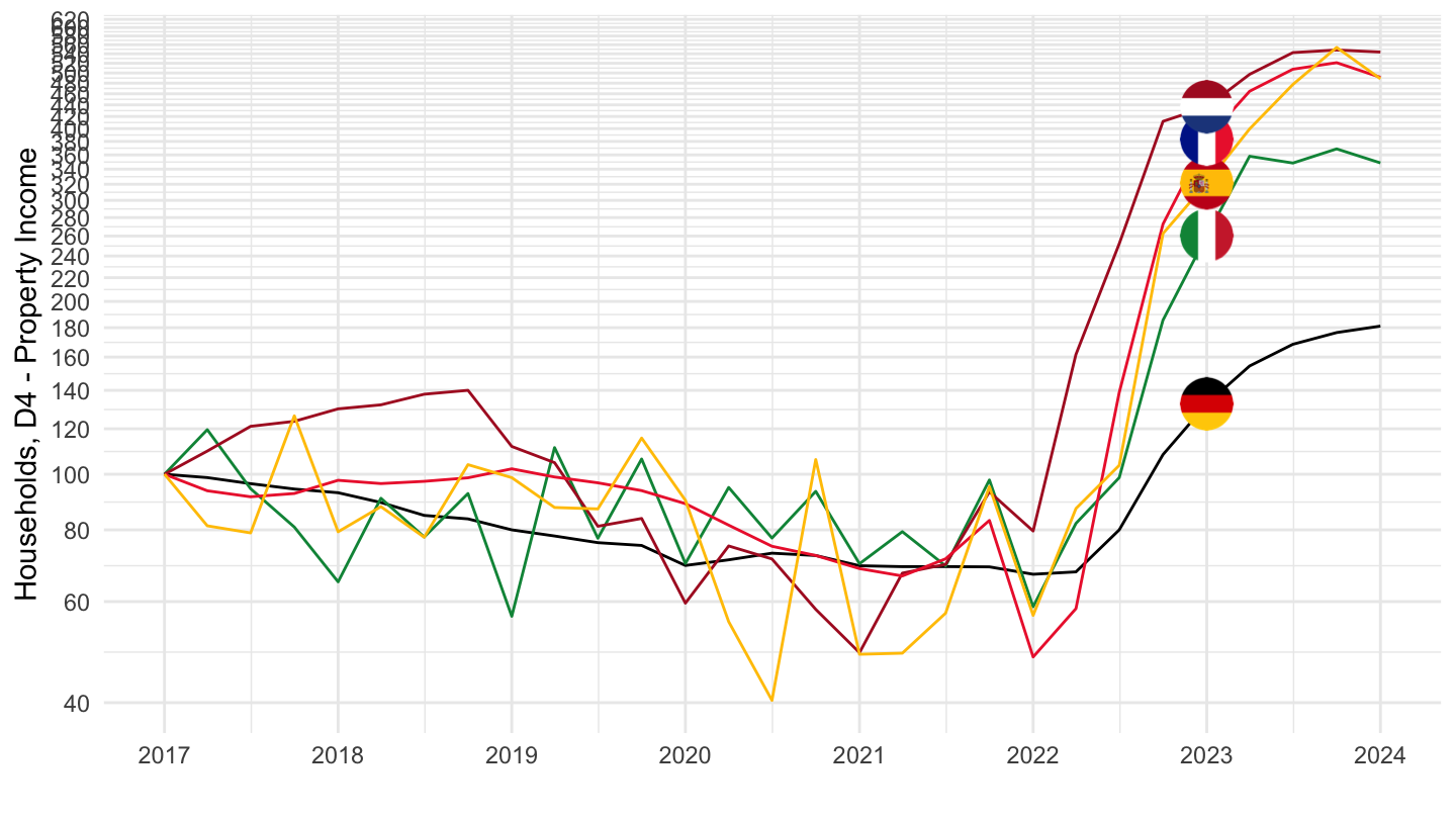
France
2017-
Table
PAID
Code
nasq_10_nf_tr %>%
  filter(geo %in% c("FR"),
         s_adj == "NSA",
         # PAID: Paid
         direct == "PAID",
         # CP_MNAC: Current prices, million units of national currency
         unit == "CP_MNAC",
         # S1: Total economy
         sector == "S14_S15",
         time %in% c("2017Q1", "2023Q3")) %>%
  left_join(na_item, by = "na_item") %>%
  select_if(~ n_distinct(.) > 1) %>%
  spread(time, values) %>%
  mutate(growth = 100*(.[[4]]/.[[3]]-1)) %>%
  #arrange(-growth) %>%
  print_table_conditional()
RECV
Code
nasq_10_nf_tr %>%
  filter(geo %in% c("FR"),
         s_adj == "NSA",
         # PAID: Paid
         direct == "RECV",
         # CP_MNAC: Current prices, million units of national currency
         unit == "CP_MNAC",
         # S1: Total economy
         sector == "S14_S15",
         time %in% c("2017Q1", "2023Q3")) %>%
  left_join(na_item, by = "na_item") %>%
  select_if(~ n_distinct(.) > 1) %>%
  spread(time, values) %>%
  mutate(growth = 100*(.[[4]]/.[[3]]-1)) %>%
  #arrange(-growth) %>%
  print_table_conditional()
Compensation of employees
Paid
Code
nasq_10_nf_tr %>%
  filter(geo %in% c("FR"),
         # B2A3G: Operating surplus and mixed income, gross
         na_item %in% c("D1"),
         # SCA: Seasonally and calendar adjusted data
         s_adj == "NSA",
         # PAID: Paid
         direct == "PAID",
         # CP_MNAC: Current prices, million units of national currency
         unit == "CP_MNAC",
         # S1: Total economy
         sector == "S14_S15") %>%
  quarter_to_date %>%
  left_join(na_item, by = "na_item") %>%
  filter(date >= as.Date("2017-01-01")) %>%
  ggplot + geom_line(aes(x = date, y = values, color = Na_item)) +
  theme_minimal()  + xlab("") + ylab("") +
  scale_x_date(breaks = as.Date(paste0(seq(1940, 2100, 1), "-01-01")),
               labels = date_format("%Y")) +
  theme(legend.position = c(0.3, 0.85),
        legend.title = element_blank()) +
  scale_y_continuous(breaks = seq(0000, 30000, 1000))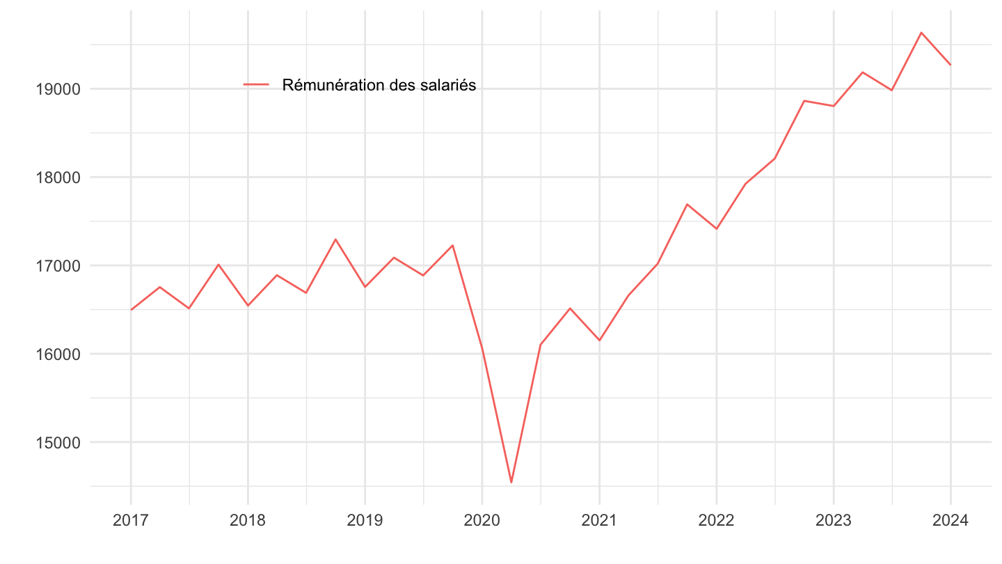
Received
Code
nasq_10_nf_tr %>%
  filter(geo %in% c("FR"),
         # B2A3G: Operating surplus and mixed income, gross
         na_item %in% c("D1"),
         # SCA: Seasonally and calendar adjusted data
         s_adj == "NSA",
         # PAID: Paid
         direct == "RECV",
         # CP_MNAC: Current prices, million units of national currency
         unit == "CP_MNAC",
         # S1: Total economy
         sector == "S14_S15") %>%
  quarter_to_date %>%
  left_join(na_item, by = "na_item") %>%
  filter(date >= as.Date("2017-01-01")) %>%
  ggplot + geom_line(aes(x = date, y = values, color = Na_item)) +
  theme_minimal()  + xlab("") + ylab("") +
  scale_x_date(breaks = as.Date(paste0(seq(1940, 2100, 1), "-01-01")),
               labels = date_format("%Y")) +
  theme(legend.position = c(0.3, 0.85),
        legend.title = element_blank()) +
  scale_y_continuous(breaks = seq(0000, 1000000, 10000))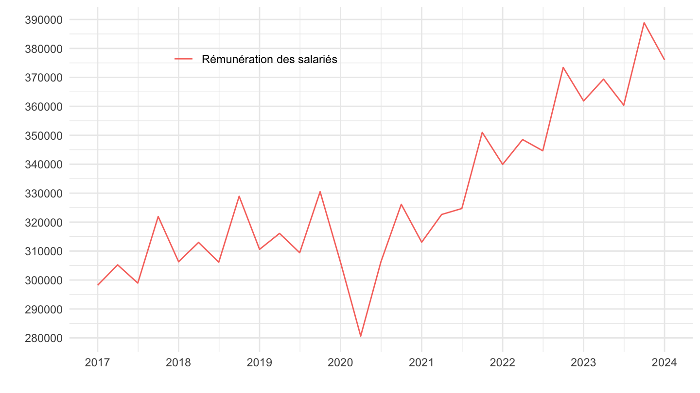
Interest
Paid
Code
nasq_10_nf_tr %>%
  filter(geo %in% c("FR"),
         # B2A3G: Operating surplus and mixed income, gross
         na_item %in% c("D4", "D41", "D41G"),
         # SCA: Seasonally and calendar adjusted data
         s_adj == "NSA",
         # PAID: Paid
         direct == "PAID",
         # CP_MNAC: Current prices, million units of national currency
         unit == "CP_MNAC",
         # S1: Total economy
         sector == "S14_S15") %>%
  quarter_to_date %>%
  left_join(na_item, by = "na_item") %>%
  filter(date >= as.Date("2017-01-01")) %>%
  ggplot + geom_line(aes(x = date, y = values, color = Na_item)) +
  theme_minimal()  + xlab("") + ylab("") +
  scale_x_date(breaks = as.Date(paste0(seq(1940, 2100, 1), "-01-01")),
               labels = date_format("%Y")) +
  theme(legend.position = c(0.3, 0.85),
        legend.title = element_blank()) +
  scale_y_continuous(breaks = seq(0000, 30000, 1000))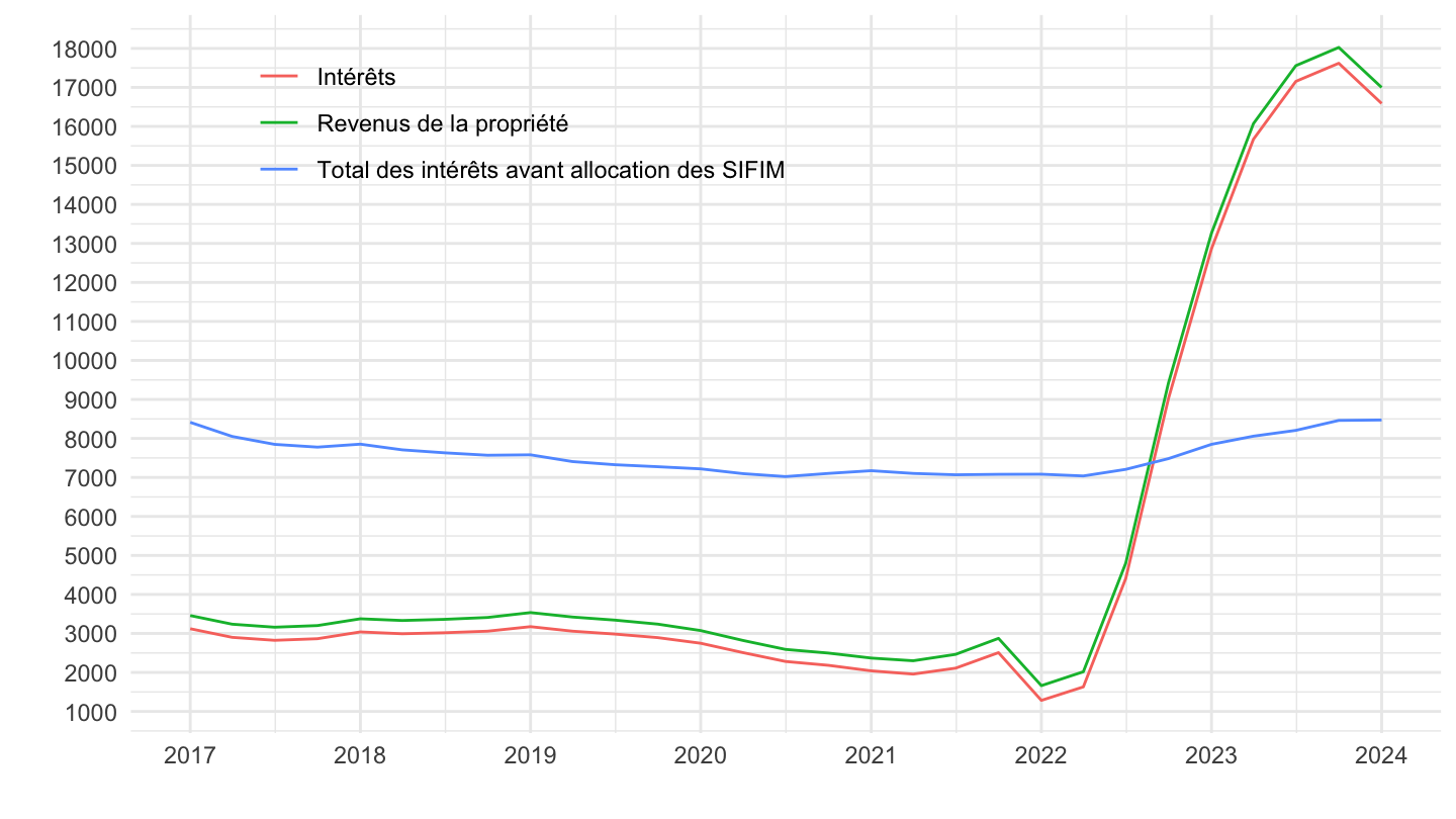
Received
Code
nasq_10_nf_tr %>%
  filter(geo %in% c("FR"),
         # B2A3G: Operating surplus and mixed income, gross
         na_item %in% c("D4", "D41", "D41G"),
         # SCA: Seasonally and calendar adjusted data
         s_adj == "NSA",
         # PAID: Paid
         direct == "RECV",
         # CP_MNAC: Current prices, million units of national currency
         unit == "CP_MNAC",
         # S1: Total economy
         sector == "S14_S15") %>%
  quarter_to_date %>%
  left_join(na_item, by = "na_item") %>%
  filter(date >= as.Date("2017-01-01")) %>%
  ggplot + geom_line(aes(x = date, y = values, color = Na_item)) +
  theme_minimal()  + xlab("") + ylab("") +
  scale_x_date(breaks = as.Date(paste0(seq(1940, 2100, 1), "-01-01")),
               labels = date_format("%Y")) +
  theme(legend.position = c(0.3, 0.85),
        legend.title = element_blank()) +
  scale_y_continuous(breaks = seq(0000, 100000, 5000))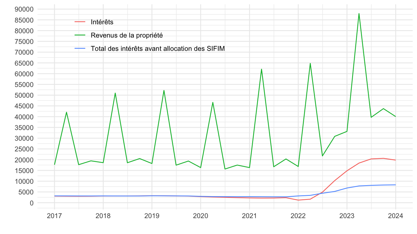
Rents
Paid
Code
nasq_10_nf_tr %>%
  filter(geo %in% c("FR"),
         # B2A3G: Operating surplus and mixed income, gross
         na_item %in% c("D42", "D43", "D44", "D45", "D42_TO_D45"),
         # SCA: Seasonally and calendar adjusted data
         s_adj == "NSA",
         # PAID: Paid
         direct == "PAID",
         # CP_MNAC: Current prices, million units of national currency
         unit == "CP_MNAC",
         # S1: Total economy
         sector == "S14_S15") %>%
  quarter_to_date %>%
  left_join(na_item, by = "na_item") %>%
  filter(date >= as.Date("2017-01-01")) %>%
  arrange(date) %>%
  ggplot + geom_line(aes(x = date, y = values, color = Na_item)) +
  theme_minimal()  + xlab("") + ylab("") +
  scale_x_date(breaks = as.Date(paste0(seq(1940, 2100, 1), "-01-01")),
               labels = date_format("%Y")) +
  theme(legend.position = c(0.3, 0.85),
        legend.title = element_blank()) +
  scale_y_continuous(breaks = seq(0000, 30000, 50))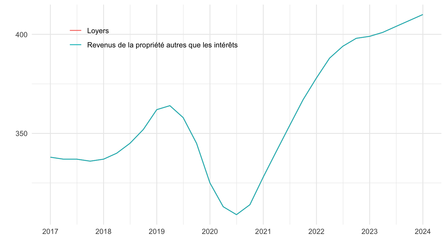
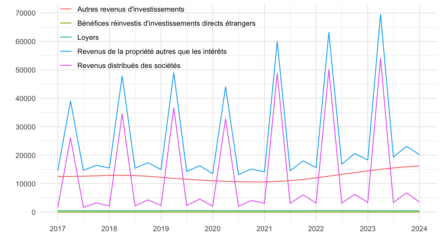
Received
Code
nasq_10_nf_tr %>%
  filter(geo %in% c("FR"),
         # B2A3G: Operating surplus and mixed income, gross
         na_item %in% c("D42", "D43", "D44", "D45", "D42_TO_D45"),
         # SCA: Seasonally and calendar adjusted data
         s_adj == "NSA",
         # PAID: Paid
         direct == "RECV",
         # CP_MNAC: Current prices, million units of national currency
         unit == "CP_MNAC",
         # S1: Total economy
         sector == "S14_S15") %>%
  quarter_to_date %>%
  left_join(na_item, by = "na_item") %>%
  filter(date >= as.Date("2017-01-01")) %>%
  arrange(date) %>%
  ggplot + geom_line(aes(x = date, y = values, color = Na_item)) +
  theme_minimal()  + xlab("") + ylab("") +
  scale_x_date(breaks = as.Date(paste0(seq(1940, 2100, 1), "-01-01")),
               labels = date_format("%Y")) +
  theme(legend.position = c(0.3, 0.85),
        legend.title = element_blank()) +
  scale_y_continuous(breaks = seq(0000, 100000, 10000))