| source | dataset | Title | .html | .rData |
|---|---|---|---|---|
| eurostat | nasa_10_nf_tr | Non-financial transactions | 2026-07-21 | 2026-07-21 |
| eurostat | nasq_10_nf_tr | Non-financial transactions | 2026-07-21 | 2026-07-21 |
Non-financial transactions
Data - Eurostat
Info
Data on europe
Code
load_data("europe.RData")
europe %>%
  arrange(-(dataset == "nasa_10_nf_tr")) %>%
source_dataset_file_updates()| source | dataset | Title | .html | .rData |
|---|---|---|---|---|
| eurostat | nasa_10_nf_tr | Non-financial transactions | 2026-07-21 | 2026-07-21 |
| eurostat | bop_gdp6_q | Main Balance of Payments and International Investment Position items as share of GDP (BPM6) | 2026-07-21 | 2026-07-21 |
| eurostat | nama_10_a10 | Gross value added and income by A*10 industry breakdowns | 2026-07-21 | 2026-07-21 |
| eurostat | nama_10_a10_e | Employment by A*10 industry breakdowns | 2026-07-21 | 2026-07-21 |
| eurostat | nama_10_gdp | GDP and main components (output, expenditure and income) | 2026-07-21 | 2026-07-21 |
| eurostat | nama_10_lp_ulc | Labour productivity and unit labour costs | 2026-07-21 | 2026-07-21 |
| eurostat | namq_10_a10 | Gross value added and income A*10 industry breakdowns | 2026-07-21 | 2026-07-21 |
| eurostat | namq_10_a10_e | Employment A*10 industry breakdowns | 2026-07-21 | 2026-07-21 |
| eurostat | namq_10_gdp | GDP and main components (output, expenditure and income) | 2026-07-21 | 2026-07-21 |
| eurostat | namq_10_lp_ulc | Labour productivity and unit labour costs | 2026-07-21 | 2026-07-21 |
| eurostat | namq_10_pc | Main GDP aggregates per capita | 2026-07-21 | 2026-07-21 |
| eurostat | nasq_10_nf_tr | Non-financial transactions | 2026-07-21 | 2026-07-21 |
| eurostat | tipsii40 | Net international investment position - quarterly data, % of GDP | 2026-07-21 | 2026-07-21 |
Info
Code
include_graphics("https://ec.europa.eu/eurostat/statistics-explained/images/e/e1/Overall_change_in_profit_share_of_non-financial_corporations%2C_2011–2021_%28percentage_points%29_NA2022_II.png")
LAST_COMPILE
| LAST_COMPILE |
|---|
| 2026-07-22 |
Last
Code
nasa_10_nf_tr %>%
  group_by(time) %>%
  summarise(Nobs = n()) %>%
  arrange(desc(time)) %>%
  head(1) %>%
print_table_conditional()| time | Nobs |
|---|---|
| 2025 | 7466 |
unit
Code
nasa_10_nf_tr %>%
  left_join(unit, by = "unit") %>%
  group_by(unit, Unit) %>%
  summarise(Nobs = n()) %>%
  arrange(-Nobs) %>%
{if (is_html_output()) print_table(.) else .}| unit | Unit | Nobs |
|---|---|---|
| CP_MNAC | Current prices, million units of national currency | 1067181 |
| CP_MEUR | Current prices, million euro | 1036645 |
| PPS_EU27_2020_HAB | Purchasing power standard (PPS, EU27 from 2020), per inhabitant | 2006 |
sector
Code
nasa_10_nf_tr %>%
  left_join(sector, by = "sector") %>%
  group_by(sector, Sector) %>%
  summarise(Nobs = n()) %>%
  arrange(-Nobs) %>%
{if (is_html_output()) print_table(.) else .}| sector | Sector | Nobs |
|---|---|---|
| S1 | Total economy | 341881 |
| S14_S15 | Households; non-profit institutions serving households | 278694 |
| S12 | Financial corporations | 235110 |
| S11 | Non-financial corporations | 229340 |
| S13 | General government | 225068 |
| S2 | Rest of the world | 224097 |
| S14 | Households | 218917 |
| S15 | Non-profit institutions serving households | 188160 |
| S128_S129 | Insurance corporations and pension funds | 44934 |
| S121_S122_S123 | Monetary financial institutions | 44794 |
| S124_TO_S127 | Other financial institutions (financial corporations other than MFIs, insurance corporations and pension funds) | 39542 |
| S1N | Not sectorised | 19333 |
| S11001 | Public non-financial corporations | 12348 |
| S12001 | Public financial corporations | 3614 |
direct
Code
nasa_10_nf_tr %>%
  left_join(direct, by = "direct") %>%
  group_by(direct, Direct) %>%
  summarise(Nobs = n()) %>%
  arrange(-Nobs) %>%
{if (is_html_output()) print_table(.) else .}| direct | Direct | Nobs |
|---|---|---|
| PAID | Paid | 1101707 |
| RECV | Received | 1004125 |
na_item
Code
nasa_10_nf_tr %>%
  left_join(na_item, by = "na_item") %>%
  group_by(na_item, Na_item) %>%
  summarise(Nobs = n()) %>%
  arrange(-Nobs) %>%
  {if (is_html_output()) datatable(., filter = 'top', rownames = F) else .}
geo
Code
nasa_10_nf_tr %>%
  left_join(geo, by = "geo") %>%
  group_by(geo, Geo) %>%
  summarise(Nobs = n()) %>%
  arrange(-Nobs) %>%
  {if (is_html_output()) datatable(., filter = 'top', rownames = F) else .}
Operating surplus and mixed income, gross
Code
nasa_10_nf_tr %>%
  filter(geo %in% c("FR", "DE", "IT"),
         # B2A3G: Operating surplus and mixed income, gross
         na_item == "B2A3G",
         # PAID: Paid
         direct == "PAID",
         # CP_MNAC: Current prices, million units of national currency
         unit == "CP_MNAC",
         # S1: Total economy
         sector == "S1") %>%
  year_to_date %>%
  ggplot + geom_line(aes(x = date, y = values/1000, color = geo, linetype = geo)) +
  scale_color_manual(values = viridis(4)[1:3]) +
  theme_minimal()  +
  scale_x_date(breaks = as.Date(paste0(seq(1940, 2100, 5), "-01-01")),
               labels = date_format("%y")) +
  theme(legend.position = c(0.2, 0.85),
        legend.title = element_blank()) +
  xlab("") + ylab("") +
  scale_y_log10(breaks = seq(0, 1000, 100),
                labels = dollar_format(suffix = " Bn€", prefix = "", accuracy = 1))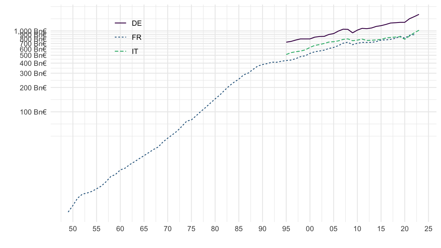
France
Imputed social contributions
All
Code
nasa_10_nf_tr %>%
  filter(na_item == "D612",
         geo == "IT") %>%
  arrange(-values) %>%
  left_join(geo, by = "geo") %>%
  left_join(gdp, by = c("geo", "time")) %>%
  mutate(values_gdp = values/gdp) %>%
  select_if(~ n_distinct(.) > 1) %>%
  print_table_conditional
2022
Code
nasa_10_nf_tr %>%
  filter(na_item == "D612",
         time == "2021",
         sector == "S13",
         direct == "RECV",
         unit == "CP_MEUR") %>%
  arrange(-values) %>%
  left_join(geo, by = "geo") %>%
  left_join(gdp, by = c("geo", "time")) %>%
  mutate(values_gdp = values/gdp) %>%
  select_if(~ n_distinct(.) > 1) %>%
print_table_conditional| geo | values | Geo | gdp | values_gdp |
|---|---|---|---|---|
| FR | 44866 | France | 2508102.3 | 0.0178884 |
| BE | 11000 | Belgium | 506047.2 | 0.0217371 |
| ES | 6932 | Spain | 1235474.0 | 0.0056108 |
| PL | 4939 | Poland | 2661518.0 | 0.0018557 |
| NL | 4525 | Netherlands | 891550.0 | 0.0050754 |
| EL | 3856 | Greece | 184574.6 | 0.0208913 |
| IE | 3697 | Ireland | 448445.1 | 0.0082440 |
| RO | 1950 | Romania | 1186015.4 | 0.0016442 |
| AT | 1567 | Austria | 406231.5 | 0.0038574 |
| LU | 891 | Luxembourg | 73039.5 | 0.0121989 |
| NO | 590 | Norway | 4480477.0 | 0.0001317 |
| CH | 524 | Switzerland | 768279.4 | 0.0006820 |
| CY | 409 | Cyprus | 25679.9 | 0.0159269 |
| DK | 403 | Denmark | 2553260.5 | 0.0001578 |
| SK | 394 | Slovakia | 101891.6 | 0.0038669 |
| LT | 183 | Lithuania | 56709.1 | 0.0032270 |
| SI | 180 | Slovenia | 52032.4 | 0.0034594 |
| LV | 142 | Latvia | 32283.8 | 0.0043985 |
| CZ | 139 | Czechia | 6307755.0 | 0.0000220 |
| MT | 104 | Malta | 16681.7 | 0.0062344 |
| EE | 96 | Estonia | 31453.3 | 0.0030521 |
| FI | 0 | Finland | 248764.0 | 0.0000000 |
| IS | 0 | Iceland | 3331536.5 | 0.0000000 |
2022
Code
nasa_10_nf_tr %>%
  filter(na_item == "D612",
         time == "2022",
         sector == "S13",
         direct == "RECV",
         unit == "CP_MEUR") %>%
  arrange(-values) %>%
  left_join(geo, by = "geo") %>%
  left_join(gdp, by = c("geo", "time")) %>%
  mutate(values_gdp = values/gdp) %>%
  select_if(~ n_distinct(.) > 1) %>%
print_table_conditional| geo | values | Geo | gdp | values_gdp |
|---|---|---|---|---|
| FR | 46474 | France | 2653997.2 | 0.0175109 |
| BE | 12032 | Belgium | 561309.1 | 0.0214356 |
| ES | 6848 | Spain | 1375863.0 | 0.0049772 |
| PL | 5366 | Poland | 3100850.0 | 0.0017305 |
| NL | 5220 | Netherlands | 993820.0 | 0.0052525 |
| IE | 4053 | Ireland | 520718.4 | 0.0077835 |
| EL | 3855 | Greece | 207008.7 | 0.0186224 |
| RO | 2146 | Romania | 1384597.8 | 0.0015499 |
| AT | 1526 | Austria | 449382.2 | 0.0033958 |
| LU | 947 | Luxembourg | 76731.2 | 0.0123418 |
| NO | 628 | Norway | 5935035.0 | 0.0001058 |
| CH | 609 | Switzerland | 819703.7 | 0.0007430 |
| SK | 401 | Slovakia | 109959.8 | 0.0036468 |
| CY | 398 | Cyprus | 29645.4 | 0.0134254 |
| DK | 397 | Denmark | 2831269.6 | 0.0001402 |
| LT | 215 | Lithuania | 67081.1 | 0.0032051 |
| CZ | 196 | Czechia | 7049872.0 | 0.0000278 |
| SI | 173 | Slovenia | 56881.6 | 0.0030414 |
| LV | 167 | Latvia | 36088.7 | 0.0046275 |
| EE | 107 | Estonia | 36300.9 | 0.0029476 |
| MT | 103 | Malta | 17984.8 | 0.0057271 |
| FI | 0 | Finland | 266135.0 | 0.0000000 |
| IS | 0 | Iceland | 3946957.2 | 0.0000000 |
2000-
Code
nasa_10_nf_tr %>%
  filter(geo %in% c("FR", "DE", "IT", "ES", "EA20"),
         na_item == "D612",
         direct == "PAID",
         unit == "CP_MNAC",
         sector == "S14_S15") %>%
  select(geo, time, values, sector) %>%
  left_join(gdp, by = c("geo", "time")) %>%
  mutate(values = values/gdp) %>%
  year_to_date %>%
  left_join(geo, by = "geo") %>%
  mutate(Geo = ifelse(geo == "EA20", "Europe", Geo)) %>%
  left_join(colors, by = c("Geo" = "country")) %>%
  filter(date >= as.Date("1995-01-01")) %>%
  ggplot + theme_minimal() + xlab("") + ylab("") +
  geom_line(aes(x = date, y = values, color = color)) +
  scale_color_identity() + add_4flags +
  scale_x_date(breaks = as.Date(paste0(seq(1940, 2100, 5), "-01-01")),
               labels = date_format("%Y")) +
  scale_y_continuous(breaks = 0.01*seq(0, 100, .2),
                labels = percent_format(a = .1))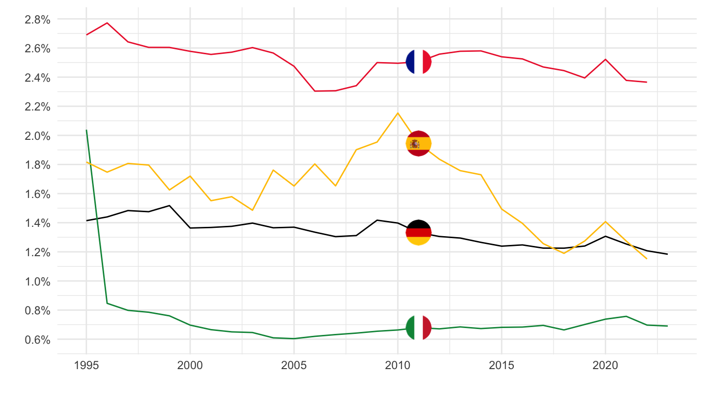
France, Germany, Italy, Spain, Europe
B6G_R_HAB
All
Code
nasa_10_nf_tr %>%
  filter(geo %in% c("FR", "DE", "IT", "ES", "EA20"),
         na_item == "B6G_R_HAB",
         direct == "PAID",
         unit == "CP_MNAC",
         sector == "S14_S15") %>%
  select(geo, time, values, sector) %>%
  year_to_date %>%
  filter(date >= as.Date("1995-01-01")) %>%
  group_by(geo) %>%
  arrange(date) %>%
  mutate(values = 100*values/values[1]) %>%
  left_join(geo, by = "geo") %>%
  mutate(Geo = ifelse(geo == "EA20", "Europe", Geo)) %>%
  left_join(colors, by = c("Geo" = "country")) %>%
  na.omit %>%
  ggplot + theme_minimal() + xlab("") + ylab("") +
  geom_line(aes(x = date, y = values, color = color)) +
  scale_color_identity() + add_5flags +
  scale_x_date(breaks = as.Date(paste0(seq(1995, 2100, 2), "-01-01")),
               labels = date_format("%Y")) +
  scale_y_continuous(breaks = seq(100, 500, 5))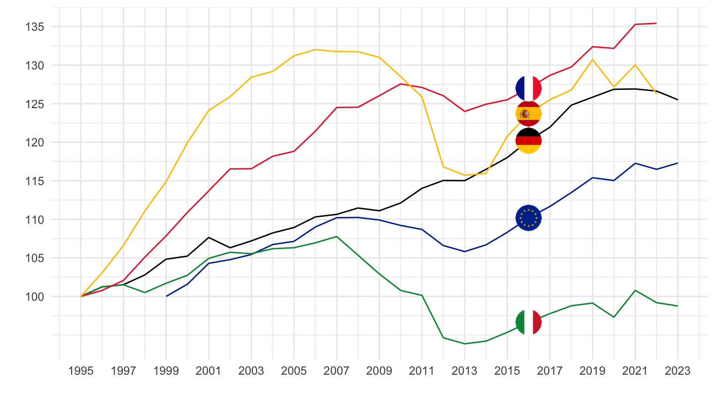
1999-
Code
nasa_10_nf_tr %>%
  filter(geo %in% c("FR", "DE", "IT", "ES", "EA20"),
         na_item == "B6G_R_HAB",
         direct == "PAID",
         unit == "CP_MNAC",
         sector == "S14_S15") %>%
  select(geo, time, values, sector) %>%
  year_to_date %>%
  filter(date >= as.Date("1999-01-01")) %>%
  group_by(geo) %>%
  arrange(date) %>%
  mutate(values = 100*values/values[1]) %>%
  left_join(geo, by = "geo") %>%
  mutate(Geo = ifelse(geo == "EA20", "Europe", Geo)) %>%
  left_join(colors, by = c("Geo" = "country")) %>%
  na.omit %>%
  ggplot + theme_minimal() + xlab("") + ylab("") +
  geom_line(aes(x = date, y = values, color = color)) +
  scale_color_identity() + add_5flags +
  scale_x_date(breaks = as.Date(paste0(seq(1995, 2100, 2), "-01-01")),
               labels = date_format("%Y")) +
  scale_y_log10(breaks = seq(10, 500, 5))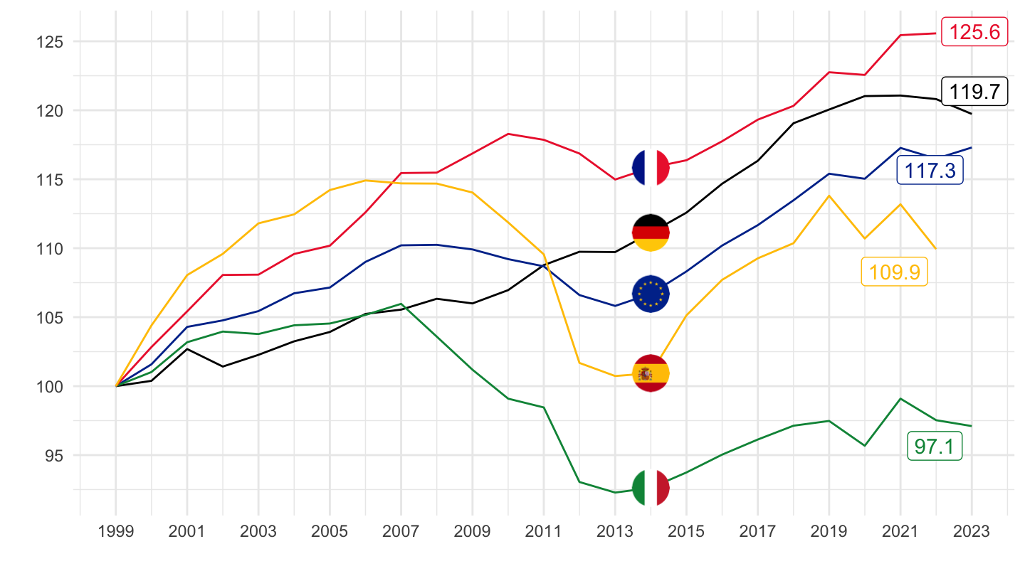
Code
#geom_label(data = . %>% filter(date == max(date)), aes(x = date, y = values, label = round(values, 1), color = color))1999- (LAbels)
Code
nasa_10_nf_tr %>%
  filter(geo %in% c("FR", "DE", "IT", "ES", "EA20"),
         na_item == "B6G_R_HAB",
         direct == "PAID",
         unit == "CP_MNAC",
         sector == "S14_S15") %>%
  select(geo, time, values, sector) %>%
  year_to_date %>%
  filter(date >= as.Date("1999-01-01")) %>%
  group_by(geo) %>%
  arrange(date) %>%
  mutate(values = 100*values/values[1]) %>%
  left_join(geo, by = "geo") %>%
  mutate(Geo = ifelse(geo == "EA20", "Europe", Geo)) %>%
  left_join(colors, by = c("Geo" = "country")) %>%
  na.omit %>%
  ggplot + theme_minimal() + xlab("") + ylab("") +
  geom_line(aes(x = date, y = values, color = color)) +
  scale_color_identity() + add_5flags +
  scale_x_date(breaks = as.Date(paste0(seq(1995, 2100, 2), "-01-01")),
               labels = date_format("%Y")) +
  scale_y_log10(breaks = seq(10, 500, 5)) +
  geom_label(data = . %>% filter(date == max(date)), aes(x = date, y = values, label = round(values, 1), color = color))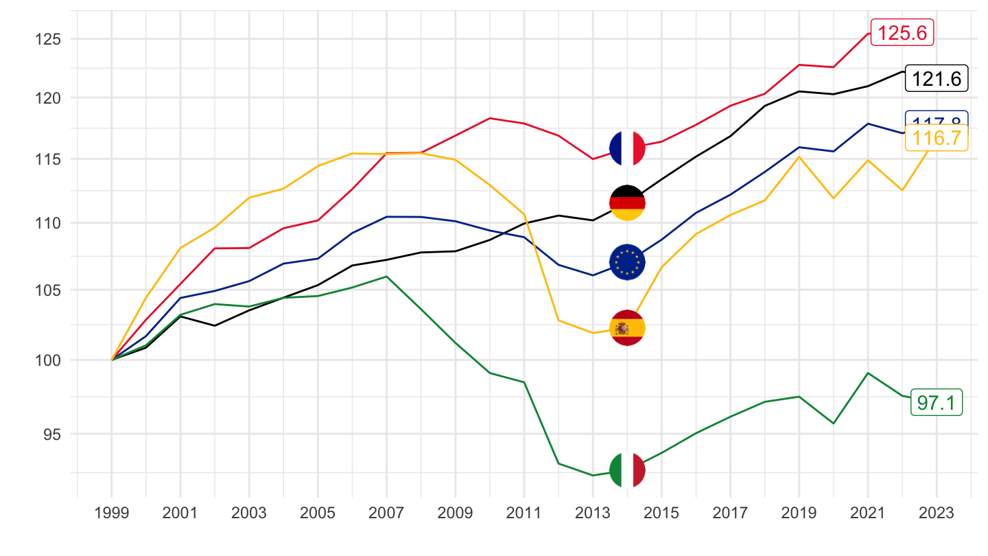
2000-
Code
nasa_10_nf_tr %>%
  filter(geo %in% c("FR", "DE", "IT", "ES", "EA20"),
         na_item == "B6G_R_HAB",
         direct == "PAID",
         unit == "CP_MNAC",
         sector == "S14_S15") %>%
  select(geo, time, values, sector) %>%
  year_to_date %>%
  filter(date >= as.Date("2000-01-01")) %>%
  group_by(geo) %>%
  arrange(date) %>%
  mutate(values = 100*values/values[1]) %>%
  left_join(geo, by = "geo") %>%
  mutate(Geo = ifelse(geo == "EA20", "Europe", Geo)) %>%
  left_join(colors, by = c("Geo" = "country")) %>%
  na.omit %>%
  ggplot + theme_minimal() + xlab("") + ylab("") +
  geom_line(aes(x = date, y = values, color = color)) +
  scale_color_identity() + add_5flags +
  scale_x_date(breaks = as.Date(paste0(seq(1995, 2100, 2), "-01-01")),
               labels = date_format("%Y")) +
  scale_y_continuous(breaks = seq(10, 500, 5)) +
  geom_label_repel(data = . %>% filter(date == max(date)), aes(x = date, y = values, label = round(values, 1), color = color))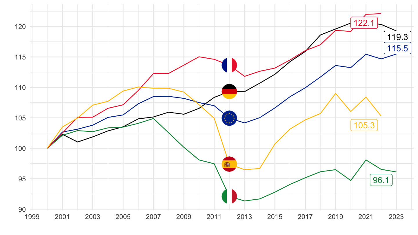
2008-
Code
nasa_10_nf_tr %>%
  filter(geo %in% c("FR", "DE", "IT", "ES", "EA20"),
         na_item == "B6G_R_HAB",
         direct == "PAID",
         unit == "CP_MNAC",
         sector == "S14_S15") %>%
  select(geo, time, values, sector) %>%
  year_to_date %>%
  filter(date >= as.Date("2008-01-01")) %>%
  group_by(geo) %>%
  arrange(date) %>%
  mutate(values = 100*values/values[1]) %>%
  left_join(geo, by = "geo") %>%
  mutate(Geo = ifelse(geo == "EA20", "Europe", Geo)) %>%
  left_join(colors, by = c("Geo" = "country")) %>%
  na.omit %>%
  ggplot + theme_minimal() + xlab("") + ylab("") +
  geom_line(aes(x = date, y = values, color = color)) +
  scale_color_identity() + add_5flags +
  scale_x_date(breaks = as.Date(paste0(seq(1995, 2100, 2), "-01-01")),
               labels = date_format("%Y")) +
  scale_y_continuous(breaks = seq(10, 500, 5)) +
  geom_label_repel(data = . %>% filter(date == max(date)), aes(x = date, y = values, label = round(values, 1), color = color))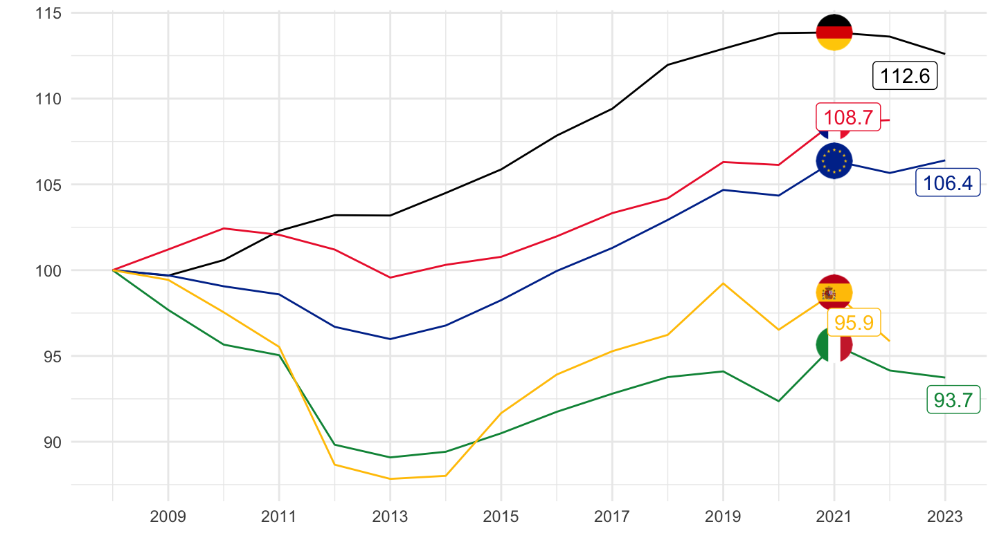
B6G
All
Code
nasa_10_nf_tr %>%
  filter(geo %in% c("FR", "DE", "IT", "ES", "EA20"),
         na_item == "B6G",
         direct == "PAID",
         unit == "CP_MNAC",
         sector == "S14_S15") %>%
  select(geo, time, values, sector) %>%
  year_to_date %>%
  filter(date >= as.Date("1995-01-01")) %>%
  group_by(geo) %>%
  arrange(date) %>%
  mutate(values = 100*values/values[1]) %>%
  left_join(geo, by = "geo") %>%
  mutate(Geo = ifelse(geo == "EA20", "Europe", Geo)) %>%
  left_join(colors, by = c("Geo" = "country")) %>%
  na.omit %>%
  ggplot + theme_minimal() + xlab("") + ylab("") +
  geom_line(aes(x = date, y = values, color = color)) +
  scale_color_identity() + add_5flags +
  scale_x_date(breaks = as.Date(paste0(seq(1995, 2100, 2), "-01-01")),
               labels = date_format("%Y")) +
  scale_y_continuous(breaks = seq(100, 500, 5))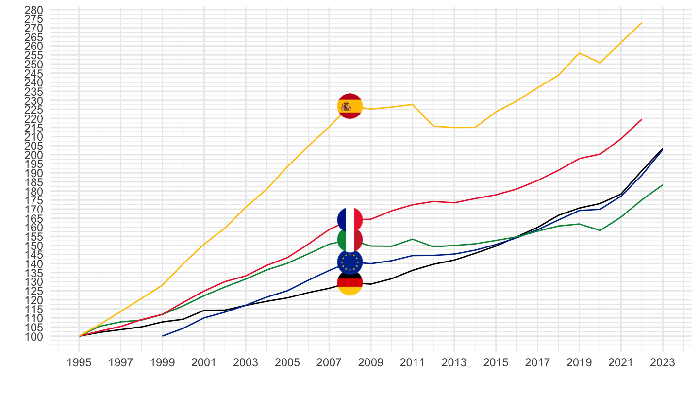
1999-
Code
nasa_10_nf_tr %>%
  filter(geo %in% c("FR", "DE", "IT", "ES", "EA20"),
         na_item == "B6G",
         direct == "PAID",
         unit == "CP_MNAC",
         sector == "S14_S15") %>%
  select(geo, time, values, sector) %>%
  year_to_date %>%
  filter(date >= as.Date("1999-01-01")) %>%
  group_by(geo) %>%
  arrange(date) %>%
  mutate(values = 100*values/values[1]) %>%
  left_join(geo, by = "geo") %>%
  mutate(Geo = ifelse(geo == "EA20", "Europe", Geo)) %>%
  left_join(colors, by = c("Geo" = "country")) %>%
  na.omit %>%
  ggplot + theme_minimal() + xlab("") + ylab("") +
  geom_line(aes(x = date, y = values, color = color)) +
  scale_color_identity() + add_5flags +
  scale_x_date(breaks = as.Date(paste0(seq(1995, 2100, 2), "-01-01")),
               labels = date_format("%Y")) +
  scale_y_log10(breaks = seq(100, 500, 5)) +
  geom_label_repel(data = . %>% filter(date == max(date)), aes(x = date, y = values, label = round(values, 1), color = color))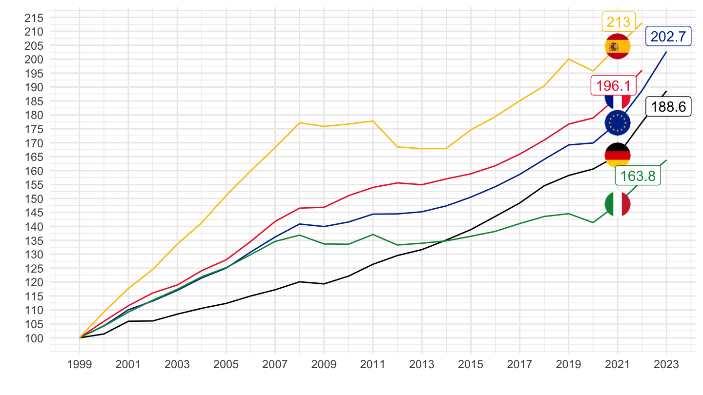
2000-
Code
nasa_10_nf_tr %>%
  filter(geo %in% c("FR", "DE", "IT", "ES", "EA20"),
         na_item == "B6G",
         direct == "PAID",
         unit == "CP_MNAC",
         sector == "S14_S15") %>%
  select(geo, time, values, sector) %>%
  year_to_date %>%
  filter(date >= as.Date("2000-01-01")) %>%
  group_by(geo) %>%
  arrange(date) %>%
  mutate(values = 100*values/values[1]) %>%
  left_join(geo, by = "geo") %>%
  mutate(Geo = ifelse(geo == "EA20", "Europe", Geo)) %>%
  left_join(colors, by = c("Geo" = "country")) %>%
  na.omit %>%
  ggplot + theme_minimal() + xlab("") + ylab("") +
  geom_line(aes(x = date, y = values, color = color)) +
  scale_color_identity() + add_5flags +
  scale_x_date(breaks = as.Date(paste0(seq(1995, 2100, 2), "-01-01")),
               labels = date_format("%Y")) +
  scale_y_continuous(breaks = seq(100, 500, 5)) +
  geom_label_repel(data = . %>% filter(date == max(date)), aes(x = date, y = values, label = round(values, 1), color = color))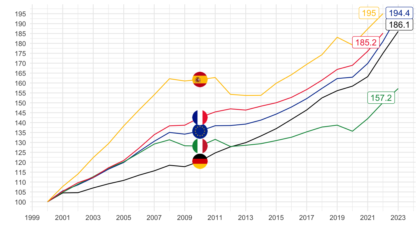
2008-
Code
nasa_10_nf_tr %>%
  filter(geo %in% c("FR", "DE", "IT", "ES", "EA20"),
         na_item == "B6G",
         direct == "PAID",
         unit == "CP_MNAC",
         sector == "S14_S15") %>%
  select(geo, time, values, sector) %>%
  year_to_date %>%
  filter(date >= as.Date("2008-01-01")) %>%
  group_by(geo) %>%
  arrange(date) %>%
  mutate(values = 100*values/values[1]) %>%
  left_join(geo, by = "geo") %>%
  mutate(Geo = ifelse(geo == "EA20", "Europe", Geo)) %>%
  left_join(colors, by = c("Geo" = "country")) %>%
  na.omit %>%
  ggplot + theme_minimal() + xlab("") + ylab("") +
  geom_line(aes(x = date, y = values, color = color)) +
  scale_color_identity() + add_5flags +
  scale_x_date(breaks = as.Date(paste0(seq(1995, 2100, 2), "-01-01")),
               labels = date_format("%Y")) +
  scale_y_continuous(breaks = seq(100, 500, 5)) +
  geom_label_repel(data = . %>% filter(date == max(date)), aes(x = date, y = values, label = round(values, 1), color = color))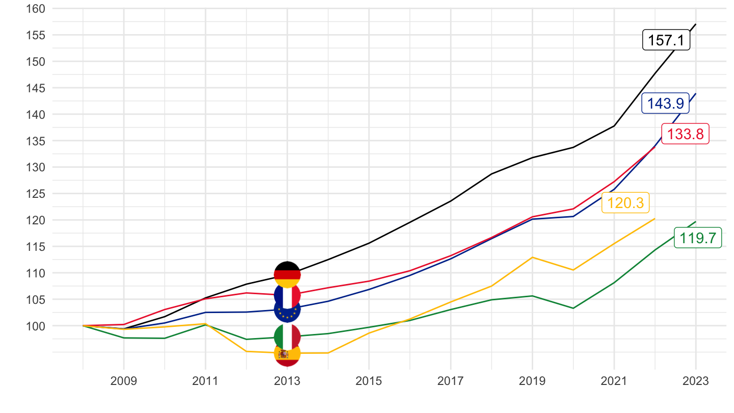
B6G/POP
All
Code
nasa_10_nf_tr %>%
  filter(geo %in% c("FR", "DE", "IT", "ES", "EA20"),
         na_item == "B6G",
         direct == "PAID",
         unit == "CP_MNAC",
         sector == "S14_S15") %>%
  select(geo, time, values, sector) %>%
  left_join(POP, by = c("geo", "time")) %>%
  mutate(values = values/POP) %>%
  year_to_date %>%
  filter(date >= as.Date("1995-01-01")) %>%
  group_by(geo) %>%
  arrange(date) %>%
  mutate(values = 100*values/values[1]) %>%
  left_join(geo, by = "geo") %>%
  mutate(Geo = ifelse(geo == "EA20", "Europe", Geo)) %>%
  left_join(colors, by = c("Geo" = "country")) %>%
  na.omit %>%
  ggplot + theme_minimal() + xlab("") + ylab("") +
  geom_line(aes(x = date, y = values, color = color)) +
  scale_color_identity() + add_5flags +
  scale_x_date(breaks = as.Date(paste0(seq(1995, 2100, 2), "-01-01")),
               labels = date_format("%Y")) +
  scale_y_continuous(breaks = seq(100, 500, 5))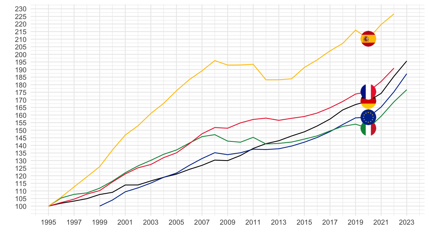
1999-
B6G/POP - labels
Code
nasa_10_nf_tr %>%
  filter(geo %in% c("FR", "DE", "IT", "ES", "EA20"),
         na_item == "B6G",
         direct == "PAID",
         unit == "CP_MNAC",
         sector == "S14_S15") %>%
  select(geo, time, values, sector) %>%
  left_join(POP, by = c("geo", "time")) %>%
  mutate(values = values/POP) %>%
  year_to_date %>%
  filter(date >= as.Date("1999-01-01")) %>%
  group_by(geo) %>%
  arrange(date) %>%
  mutate(values = 100*values/values[1]) %>%
  left_join(geo, by = "geo") %>%
  mutate(Geo = ifelse(geo == "EA20", "Europe", Geo)) %>%
  left_join(colors, by = c("Geo" = "country")) %>%
  na.omit %>%
  ggplot + theme_minimal() + xlab("") + ylab("") +
  geom_line(aes(x = date, y = values, color = color)) +
  scale_color_identity() + add_5flags +
  scale_x_date(breaks = as.Date(paste0(seq(1995, 2100, 2), "-01-01")),
               labels = date_format("%Y")) +
  scale_y_continuous(breaks = seq(100, 500, 5)) +
  geom_label_repel(data = . %>% filter(date == max(date)), aes(x = date, y = values, label = round(values, 1), color = color))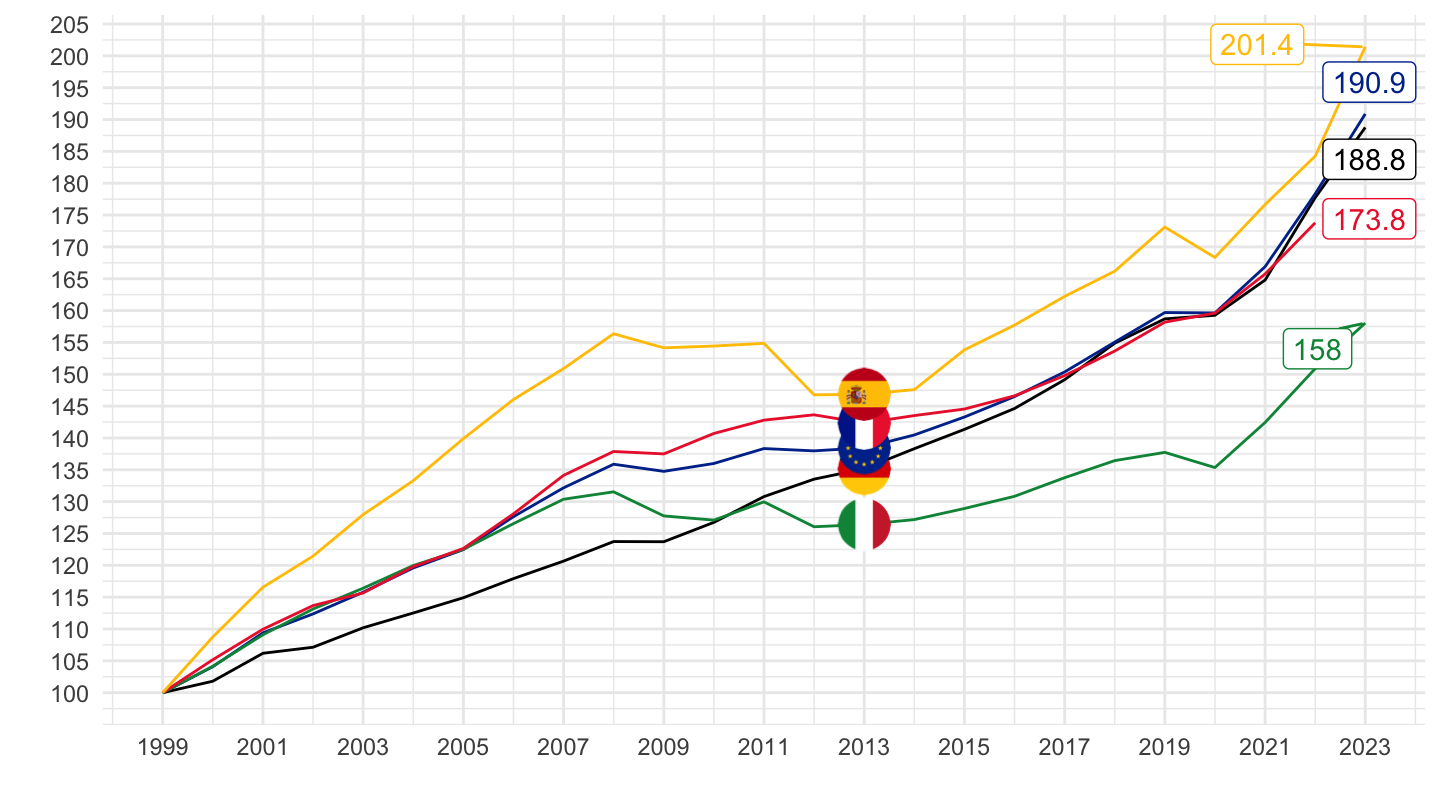
B6G/POP
Code
nasa_10_nf_tr %>%
  filter(geo %in% c("FR", "DE", "IT", "ES", "EA20"),
         na_item == "B6G",
         direct == "PAID",
         unit == "CP_MNAC",
         sector == "S14_S15") %>%
  select(geo, time, values, sector) %>%
  left_join(POP, by = c("geo", "time")) %>%
  mutate(values = values/POP) %>%
  year_to_date %>%
  filter(date >= as.Date("1999-01-01")) %>%
  group_by(geo) %>%
  arrange(date) %>%
  mutate(values = 100*values/values[1]) %>%
  left_join(geo, by = "geo") %>%
  mutate(Geo = ifelse(geo == "EA20", "Europe", Geo)) %>%
  left_join(colors, by = c("Geo" = "country")) %>%
  na.omit %>%
  ggplot + theme_minimal() + xlab("") + ylab("") +
  geom_line(aes(x = date, y = values, color = color)) +
  scale_color_identity() + add_5flags +
  scale_x_date(breaks = as.Date(paste0(seq(1995, 2100, 2), "-01-01")),
               labels = date_format("%Y")) +
  scale_y_continuous(breaks = seq(100, 500, 5))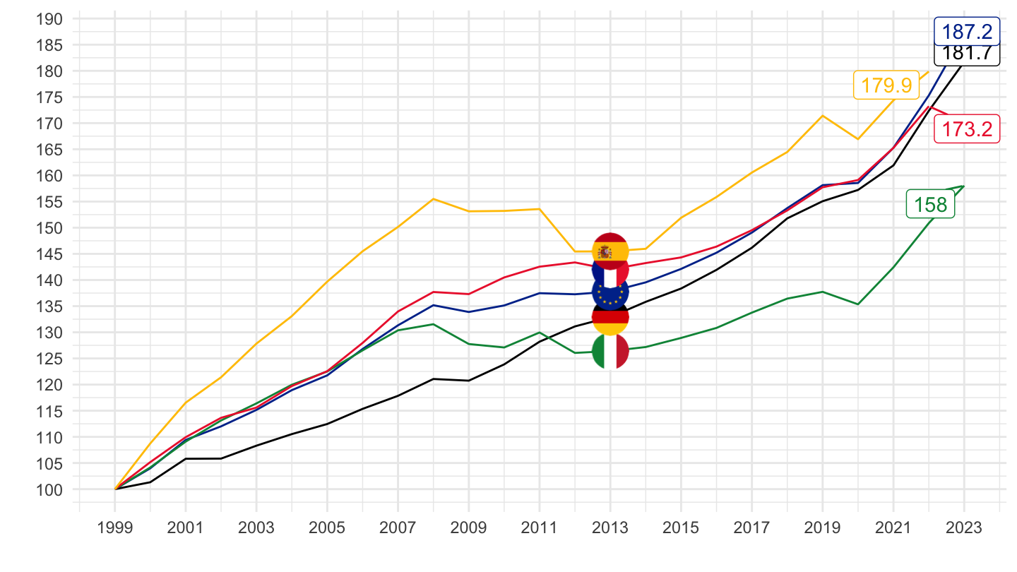
Code
#geom_label_repel(data = . %>% filter(date == max(date)), aes(x = date, y = values, label = round(values, 1), color = color))D11/POP
Code
nasa_10_nf_tr %>%
  filter(geo %in% c("FR", "DE", "IT", "ES", "EA20"),
         na_item == "D11",
         direct == "PAID",
         unit == "CP_MNAC",
         sector == "S14_S15") %>%
  select(geo, time, values, sector) %>%
  left_join(POP, by = c("geo", "time")) %>%
  mutate(values = values/POP) %>%
  year_to_date %>%
  filter(date >= as.Date("1999-01-01")) %>%
  group_by(geo) %>%
  arrange(date) %>%
  mutate(values = 100*values/values[1]) %>%
  left_join(geo, by = "geo") %>%
  mutate(Geo = ifelse(geo == "EA20", "Europe", Geo)) %>%
  left_join(colors, by = c("Geo" = "country")) %>%
  na.omit %>%
  ggplot + theme_minimal() + xlab("") + ylab("") +
  geom_line(aes(x = date, y = values, color = color)) +
  scale_color_identity() + add_5flags +
  scale_x_date(breaks = as.Date(paste0(seq(1995, 2100, 2), "-01-01")),
               labels = date_format("%Y")) +
  scale_y_continuous(breaks = seq(100, 500, 5)) +
  geom_label_repel(data = . %>% filter(date == max(date)), aes(x = date, y = values, label = round(values, 1), color = color))
B7G_R_HAB
Code
nasa_10_nf_tr %>%
  filter(geo %in% c("FR", "DE", "IT", "ES", "EA20"),
         na_item == "B7G_R_HAB",
         direct == "PAID",
         unit == "CP_MNAC",
         sector == "S14_S15") %>%
  select(geo, time, values, sector) %>%
  year_to_date %>%
  filter(date >= as.Date("1999-01-01")) %>%
  group_by(geo) %>%
  arrange(date) %>%
  mutate(values = 100*values/values[1]) %>%
  left_join(geo, by = "geo") %>%
  mutate(Geo = ifelse(geo == "EA20", "Europe", Geo)) %>%
  left_join(colors, by = c("Geo" = "country")) %>%
  na.omit %>%
  ggplot + theme_minimal() + xlab("") + ylab("") +
  geom_line(aes(x = date, y = values, color = color)) +
  scale_color_identity() + add_5flags +
  scale_x_date(breaks = as.Date(paste0(seq(1995, 2100, 2), "-01-01")),
               labels = date_format("%Y")) +
  scale_y_continuous(breaks = seq(10, 500, 5)) +
  geom_label_repel(data = . %>% filter(date == max(date)), aes(x = date, y = values, label = round(values, 1), color = color))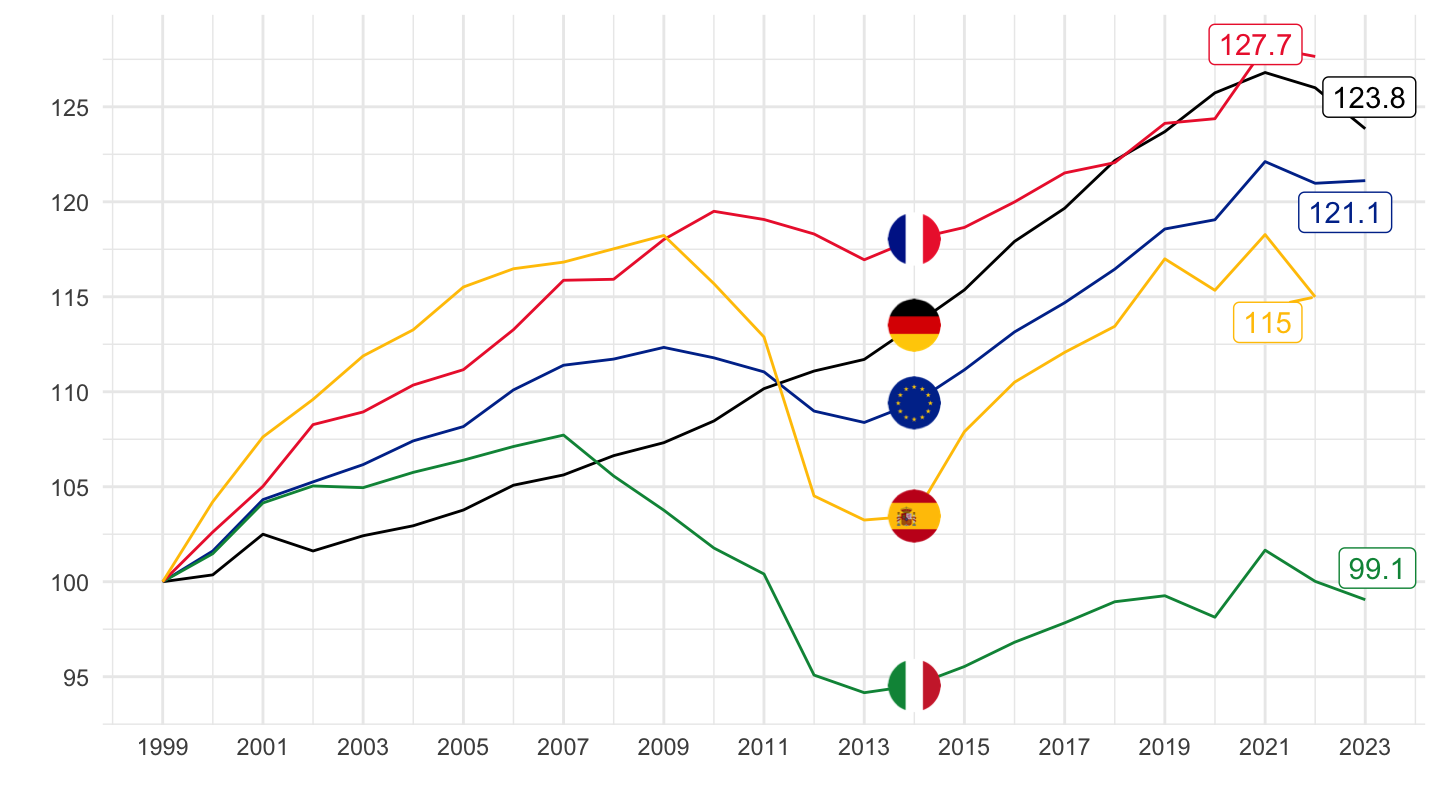
D41/POP
Code
nasa_10_nf_tr %>%
  filter(geo %in% c("FR", "DE", "IT", "ES", "EA20"),
         na_item == "D41",
         direct == "PAID",
         unit == "CP_MNAC",
         sector == "S14_S15") %>%
  select(geo, time, values, sector) %>%
  left_join(POP, by = c("geo", "time")) %>%
  mutate(values = values/POP) %>%
  year_to_date %>%
  filter(date >= as.Date("1999-01-01")) %>%
  group_by(geo) %>%
  arrange(date) %>%
  mutate(values = 100*values/values[1]) %>%
  left_join(geo, by = "geo") %>%
  mutate(Geo = ifelse(geo == "EA20", "Europe", Geo)) %>%
  left_join(colors, by = c("Geo" = "country")) %>%
  na.omit %>%
  ggplot + theme_minimal() + xlab("") + ylab("") +
  geom_line(aes(x = date, y = values, color = color)) +
  scale_color_identity() + add_5flags +
  scale_x_date(breaks = as.Date(paste0(seq(1995, 2100, 2), "-01-01")),
               labels = date_format("%Y")) +
  scale_y_continuous(breaks = seq(100, 500, 5)) +
  geom_label_repel(data = . %>% filter(date == max(date)), aes(x = date, y = values, label = round(values, 1), color = color))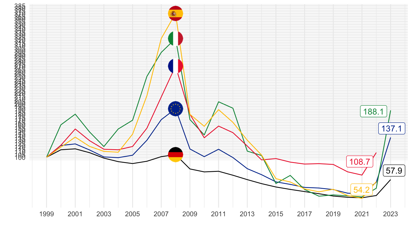
D4/POP
Code
nasa_10_nf_tr %>%
  filter(geo %in% c("FR", "DE", "IT", "ES", "EA20"),
         na_item == "D4",
         direct == "PAID",
         unit == "CP_MNAC",
         sector == "S14_S15") %>%
  select(geo, time, values, sector) %>%
  left_join(POP, by = c("geo", "time")) %>%
  mutate(values = values/POP) %>%
  year_to_date %>%
  filter(date >= as.Date("1999-01-01")) %>%
  group_by(geo) %>%
  arrange(date) %>%
  mutate(values = 100*values/values[1]) %>%
  left_join(geo, by = "geo") %>%
  mutate(Geo = ifelse(geo == "EA20", "Europe", Geo)) %>%
  left_join(colors, by = c("Geo" = "country")) %>%
  na.omit %>%
  ggplot + theme_minimal() + xlab("") + ylab("") +
  geom_line(aes(x = date, y = values, color = color)) +
  scale_color_identity() + add_5flags +
  scale_x_date(breaks = as.Date(paste0(seq(1995, 2100, 2), "-01-01")),
               labels = date_format("%Y")) +
  scale_y_continuous(breaks = seq(100, 500, 5)) +
  geom_label_repel(data = . %>% filter(date == max(date)), aes(x = date, y = values, label = round(values, 1), color = color))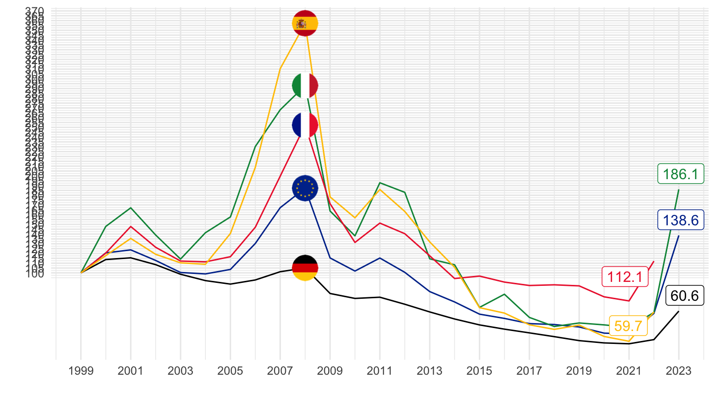
2000-
Code
nasa_10_nf_tr %>%
  filter(geo %in% c("FR", "DE", "IT", "ES", "EA20"),
         na_item == "B6G",
         direct == "PAID",
         unit == "CP_MNAC",
         sector == "S14_S15") %>%
  select(geo, time, values, sector) %>%
  left_join(POP, by = c("geo", "time")) %>%
  mutate(values = values/POP) %>%
  year_to_date %>%
  filter(date >= as.Date("2000-01-01")) %>%
  group_by(geo) %>%
  arrange(date) %>%
  mutate(values = 100*values/values[1]) %>%
  left_join(geo, by = "geo") %>%
  mutate(Geo = ifelse(geo == "EA20", "Europe", Geo)) %>%
  left_join(colors, by = c("Geo" = "country")) %>%
  na.omit %>%
  ggplot + theme_minimal() + xlab("") + ylab("") +
  geom_line(aes(x = date, y = values, color = color)) +
  scale_color_identity() + add_5flags +
  scale_x_date(breaks = as.Date(paste0(seq(1995, 2100, 2), "-01-01")),
               labels = date_format("%Y")) +
  scale_y_continuous(breaks = seq(100, 500, 5)) +
  geom_label_repel(data = . %>% filter(date == max(date)), aes(x = date, y = values, label = round(values, 1), color = color))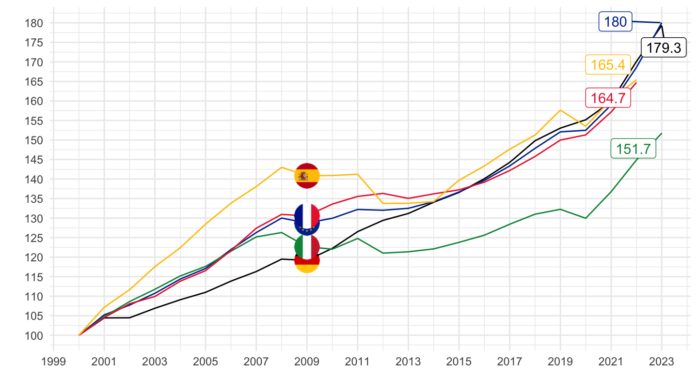
2008-
Code
nasa_10_nf_tr %>%
  filter(geo %in% c("FR", "DE", "IT", "ES", "EA20"),
         na_item == "B6G",
         direct == "PAID",
         unit == "CP_MNAC",
         sector == "S14_S15") %>%
  select(geo, time, values, sector) %>%
  left_join(POP, by = c("geo", "time")) %>%
  mutate(values = values/POP) %>%
  year_to_date %>%
  filter(date >= as.Date("2008-01-01")) %>%
  group_by(geo) %>%
  arrange(date) %>%
  mutate(values = 100*values/values[1]) %>%
  left_join(geo, by = "geo") %>%
  mutate(Geo = ifelse(geo == "EA20", "Europe", Geo)) %>%
  left_join(colors, by = c("Geo" = "country")) %>%
  na.omit %>%
  ggplot + theme_minimal() + xlab("") + ylab("") +
  geom_line(aes(x = date, y = values, color = color)) +
  scale_color_identity() + add_5flags +
  scale_x_date(breaks = as.Date(paste0(seq(1995, 2100, 2), "-01-01")),
               labels = date_format("%Y")) +
  scale_y_continuous(breaks = seq(100, 500, 5)) +
  geom_label_repel(data = . %>% filter(date == max(date)), aes(x = date, y = values, label = round(values, 1), color = color))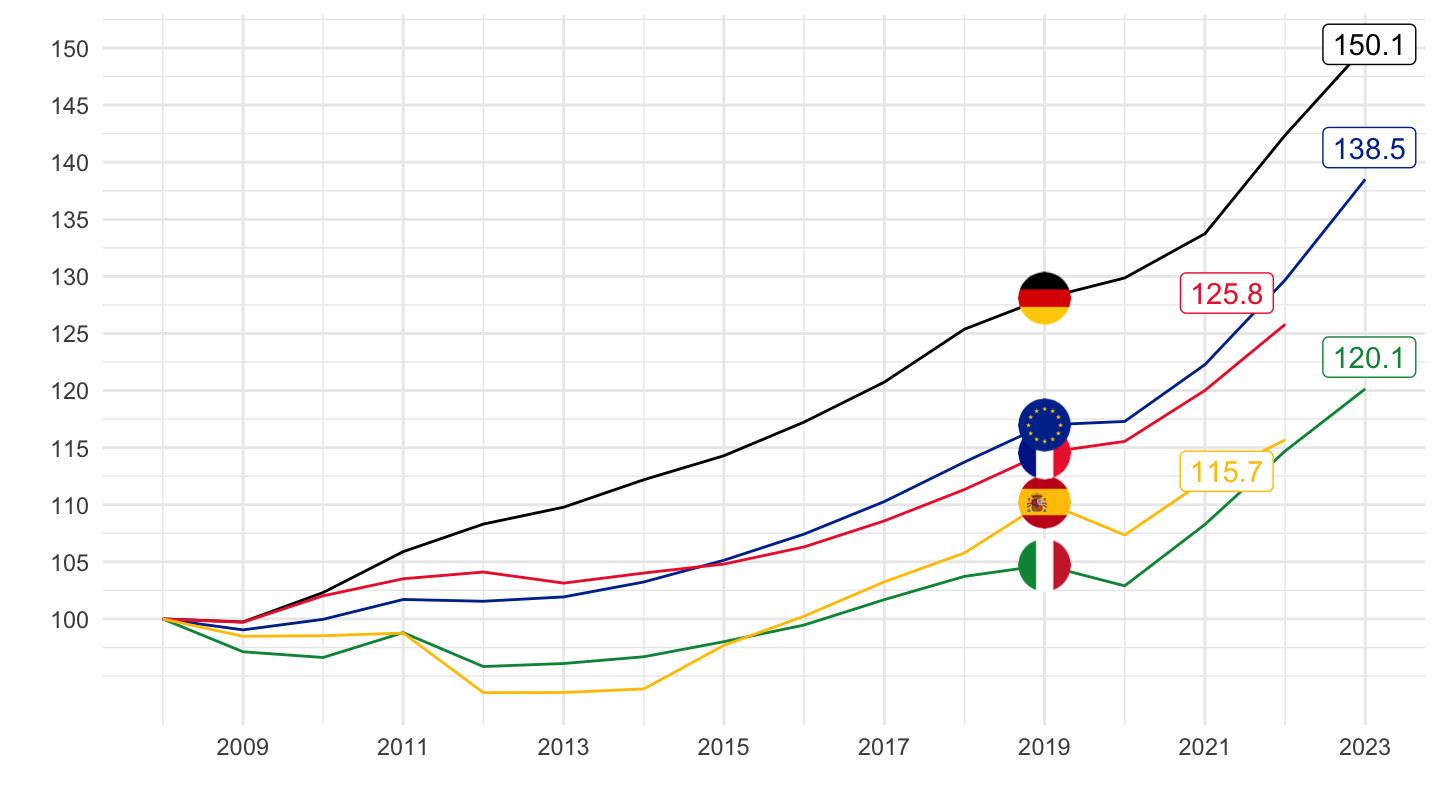
B6N
All
Code
nasa_10_nf_tr %>%
  filter(geo %in% c("FR", "DE", "IT", "ES", "EA20"),
         na_item == "B6N",
         direct == "PAID",
         unit == "CP_MNAC",
         sector == "S14_S15") %>%
  select(geo, time, values, sector) %>%
  year_to_date %>%
  #filter(date >= as.Date("1995-01-01")) %>%
  group_by(geo) %>%
  arrange(date) %>%
  mutate(values = 100*values/values[1]) %>%
  left_join(geo, by = "geo") %>%
  mutate(Geo = ifelse(geo == "EA20", "Europe", Geo)) %>%
  left_join(colors, by = c("Geo" = "country")) %>%
  na.omit %>%
  ggplot + theme_minimal() + xlab("") + ylab("") +
  geom_line(aes(x = date, y = values, color = color)) +
  scale_color_identity() + add_5flags +
  scale_x_date(breaks = as.Date(paste0(seq(1995, 2100, 2), "-01-01")),
               labels = date_format("%Y")) +
  scale_y_continuous(breaks = seq(100, 500, 5)) +
  geom_label_repel(data = . %>% filter(date == max(date)), aes(x = date, y = values, label = round(values, 1), color = color))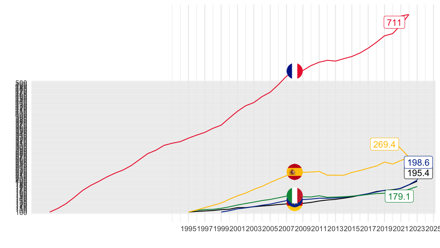
1995-
Code
nasa_10_nf_tr %>%
  filter(geo %in% c("FR", "DE", "IT", "ES", "EA20"),
         na_item == "B6N",
         direct == "PAID",
         unit == "CP_MNAC",
         sector == "S14_S15") %>%
  select(geo, time, values, sector) %>%
  year_to_date %>%
  filter(date >= as.Date("1995-01-01")) %>%
  group_by(geo) %>%
  arrange(date) %>%
  mutate(values = 100*values/values[1]) %>%
  left_join(geo, by = "geo") %>%
  mutate(Geo = ifelse(geo == "EA20", "Europe", Geo)) %>%
  left_join(colors, by = c("Geo" = "country")) %>%
  na.omit %>%
  ggplot + theme_minimal() + xlab("") + ylab("") +
  geom_line(aes(x = date, y = values, color = color)) +
  scale_color_identity() + add_5flags +
  scale_x_date(breaks = as.Date(paste0(seq(1995, 2100, 2), "-01-01")),
               labels = date_format("%Y")) +
  scale_y_continuous(breaks = seq(100, 500, 5)) +
  geom_label_repel(data = . %>% filter(date == max(date)), aes(x = date, y = values, label = round(values, 1), color = color))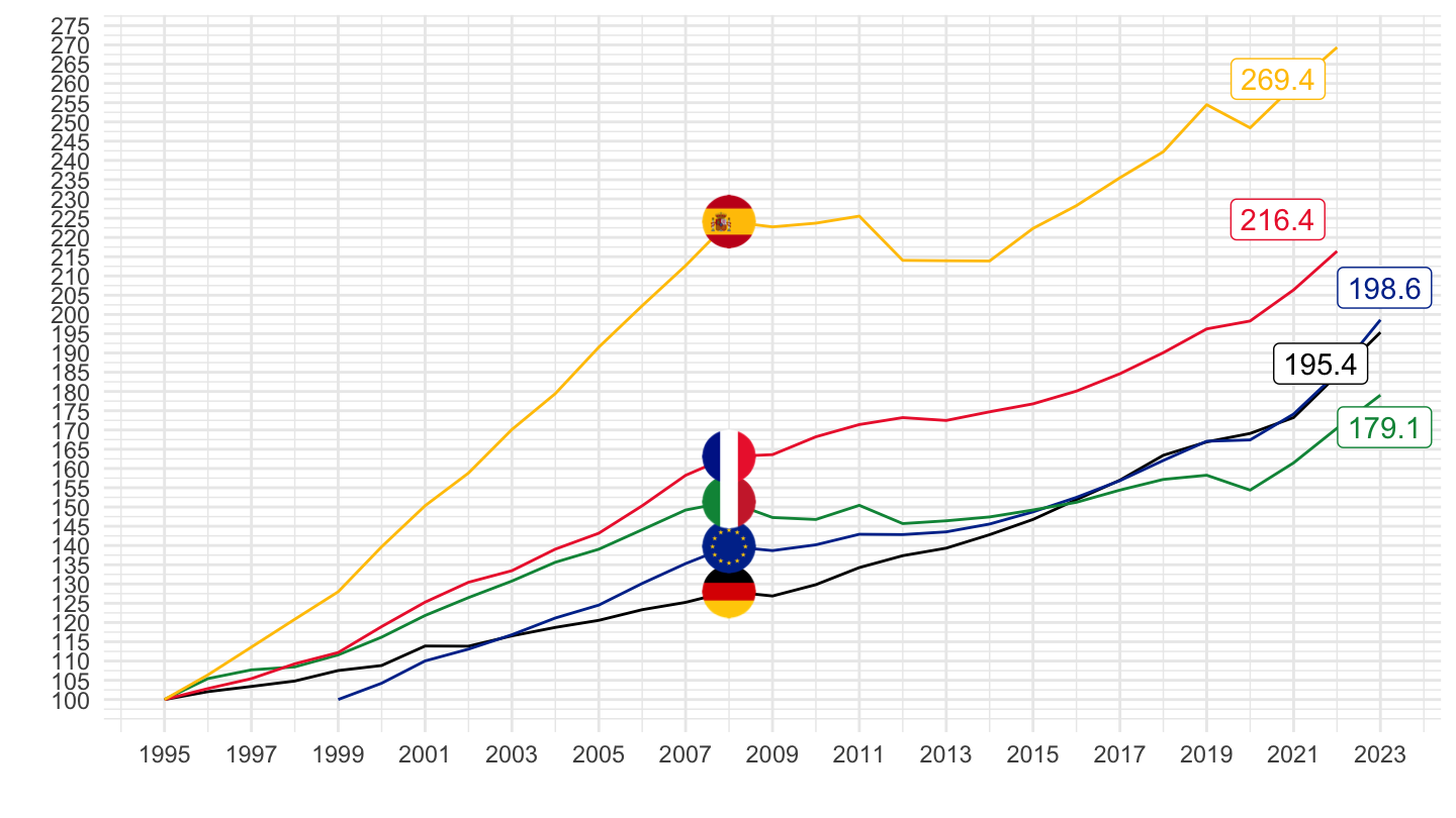
1999-
Code
nasa_10_nf_tr %>%
  filter(geo %in% c("FR", "DE", "IT", "ES", "EA20"),
         na_item == "B6N",
         direct == "PAID",
         unit == "CP_MNAC",
         sector == "S14_S15") %>%
  select(geo, time, values, sector) %>%
  year_to_date %>%
  filter(date >= as.Date("1999-01-01")) %>%
  group_by(geo) %>%
  arrange(date) %>%
  mutate(values = 100*values/values[1]) %>%
  left_join(geo, by = "geo") %>%
  mutate(Geo = ifelse(geo == "EA20", "Europe", Geo)) %>%
  left_join(colors, by = c("Geo" = "country")) %>%
  na.omit %>%
  ggplot + theme_minimal() + xlab("") + ylab("") +
  geom_line(aes(x = date, y = values, color = color)) +
  scale_color_identity() + add_5flags +
  scale_x_date(breaks = as.Date(paste0(seq(1995, 2100, 2), "-01-01")),
               labels = date_format("%Y")) +
  scale_y_continuous(breaks = seq(100, 500, 5)) +
  geom_label_repel(data = . %>% filter(date == max(date)), aes(x = date, y = values, label = round(values, 1), color = color))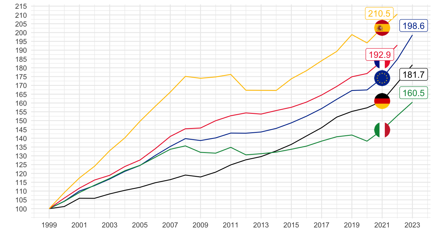
Saving Rate (B9)
All
Code
nasa_10_nf_tr %>%
  filter(geo %in% c("FR", "DE", "IT", "ES", "EA20"),
         na_item == "B9",
         direct == "PAID",
         unit == "CP_MNAC",
         sector == "S14_S15") %>%
  select(geo, time, values, sector) %>%
  left_join(gdp, by = c("geo", "time")) %>%
  mutate(values = values/gdp) %>%
  year_to_date %>%
  left_join(geo, by = "geo") %>%
  mutate(Geo = ifelse(geo == "EA20", "Europe", Geo)) %>%
  left_join(colors, by = c("Geo" = "country")) %>%
  na.omit %>%
  ggplot + theme_minimal() + xlab("") + ylab("") +
  geom_line(aes(x = date, y = values, color = color)) +
  scale_color_identity() + add_5flags +
  scale_x_date(breaks = as.Date(paste0(seq(1940, 2100, 10), "-01-01")),
               labels = date_format("%Y")) +
  scale_y_continuous(breaks = 0.01*seq(-100, 100, 1),
                labels = percent_format(a = 1))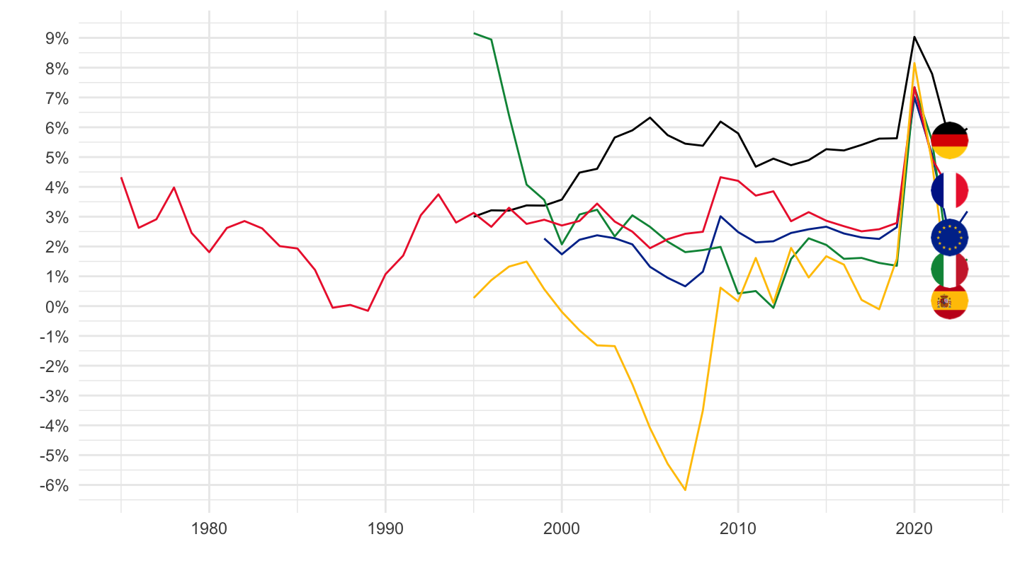
2000-
Code
nasa_10_nf_tr %>%
  filter(geo %in% c("FR", "DE", "IT", "ES", "EA20"),
         na_item == "B9",
         direct == "PAID",
         unit == "CP_MNAC",
         sector == "S14_S15") %>%
  select(geo, time, values, sector) %>%
  left_join(gdp, by = c("geo", "time")) %>%
  mutate(values = values/gdp) %>%
  year_to_date %>%
  left_join(geo, by = "geo") %>%
  mutate(Geo = ifelse(geo == "EA20", "Europe", Geo)) %>%
  left_join(colors, by = c("Geo" = "country")) %>%
  filter(date >= as.Date("2000-01-01")) %>%
  ggplot + theme_minimal() + xlab("") + ylab("") +
  geom_line(aes(x = date, y = values, color = color)) +
  scale_color_identity() + add_5flags +
  scale_x_date(breaks = as.Date(paste0(seq(1940, 2100, 2), "-01-01")),
               labels = date_format("%Y")) +
  scale_y_continuous(breaks = 0.01*seq(-100, 100, 1),
                labels = percent_format(a = 1))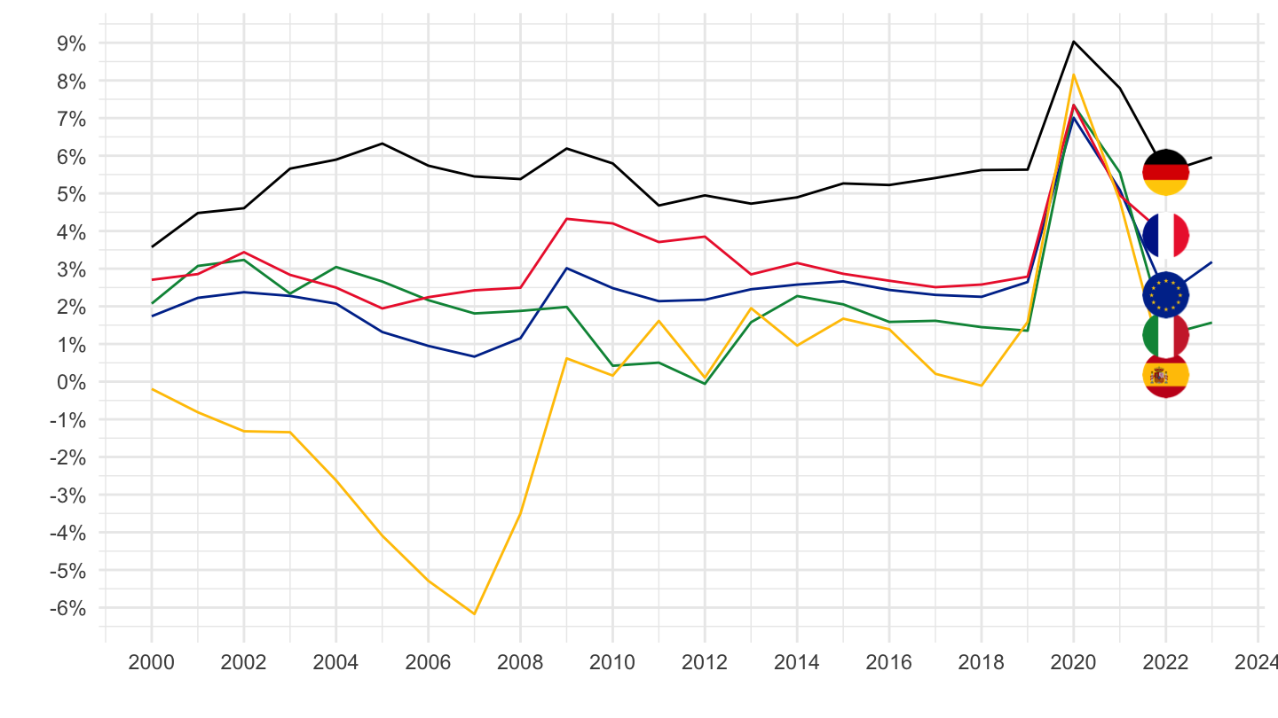
2015-
Code
nasa_10_nf_tr %>%
  filter(geo %in% c("FR", "DE", "IT", "ES", "EA20"),
         na_item == "B9",
         direct == "PAID",
         unit == "CP_MNAC",
         sector == "S14_S15") %>%
  select(geo, time, values, sector) %>%
  left_join(gdp, by = c("geo", "time")) %>%
  mutate(values = values/gdp) %>%
  year_to_date %>%
  left_join(geo, by = "geo") %>%
  mutate(Geo = ifelse(geo == "EA20", "Europe", Geo)) %>%
  left_join(colors, by = c("Geo" = "country")) %>%
  filter(date >= as.Date("2015-01-01")) %>%
  ggplot + theme_minimal() + xlab("") + ylab("") +
  geom_line(aes(x = date, y = values, color = color)) +
  scale_color_identity() + add_5flags +
  scale_x_date(breaks = as.Date(paste0(seq(1940, 2100, 1), "-01-01")),
               labels = date_format("%Y")) +
  scale_y_continuous(breaks = 0.01*seq(0, 100, 1),
                labels = percent_format(a = 1))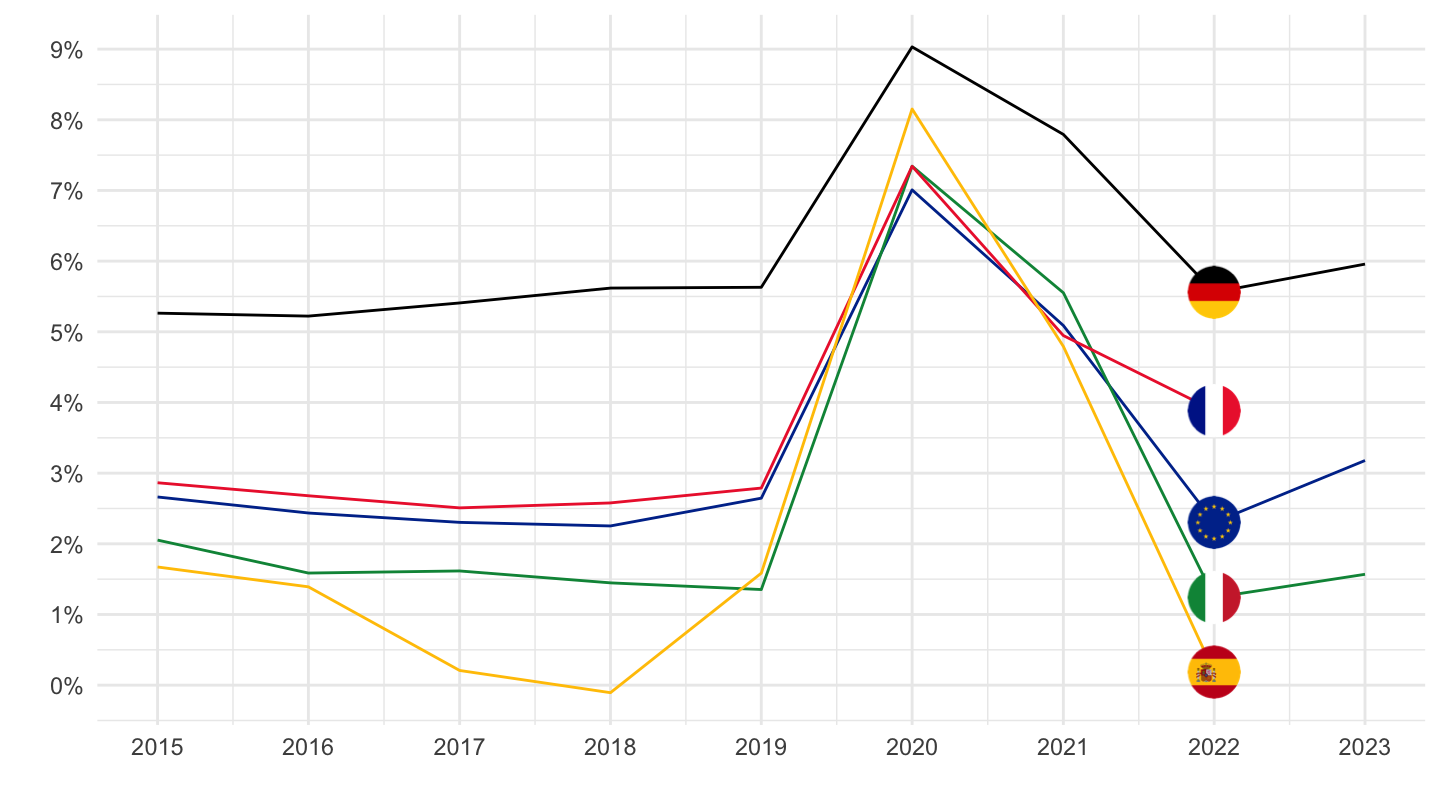
Saving Rate (B8G)
All
Code
nasa_10_nf_tr %>%
  filter(geo %in% c("FR", "DE", "IT", "ES", "EA20"),
         na_item == "B8G",
         direct == "PAID",
         unit == "CP_MNAC",
         sector == "S14_S15") %>%
  select(geo, time, values, sector) %>%
  left_join(gdp, by = c("geo", "time")) %>%
  mutate(values = values/gdp) %>%
  year_to_date %>%
  left_join(geo, by = "geo") %>%
  mutate(Geo = ifelse(geo == "EA20", "Europe", Geo)) %>%
  left_join(colors, by = c("Geo" = "country")) %>%
  na.omit %>%
  ggplot + theme_minimal() + xlab("") + ylab("") +
  geom_line(aes(x = date, y = values, color = color)) +
  scale_color_identity() + add_5flags +
  scale_x_date(breaks = as.Date(paste0(seq(1940, 2100, 10), "-01-01")),
               labels = date_format("%Y")) +
  scale_y_continuous(breaks = 0.01*seq(0, 100, 1),
                labels = percent_format(a = 1))
2000-
Code
nasa_10_nf_tr %>%
  filter(geo %in% c("FR", "DE", "IT", "ES", "EA20"),
         na_item == "B8G",
         direct == "PAID",
         unit == "CP_MNAC",
         sector == "S14_S15") %>%
  select(geo, time, values, sector) %>%
  left_join(gdp, by = c("geo", "time")) %>%
  mutate(values = values/gdp) %>%
  year_to_date %>%
  left_join(geo, by = "geo") %>%
  mutate(Geo = ifelse(geo == "EA20", "Europe", Geo)) %>%
  left_join(colors, by = c("Geo" = "country")) %>%
  filter(date >= as.Date("2000-01-01")) %>%
  ggplot + theme_minimal() + xlab("") + ylab("") +
  geom_line(aes(x = date, y = values, color = color)) +
  scale_color_identity() + add_5flags +
  scale_x_date(breaks = as.Date(paste0(seq(1940, 2100, 2), "-01-01")),
               labels = date_format("%Y")) +
  scale_y_continuous(breaks = 0.01*seq(0, 100, 1),
                labels = percent_format(a = 1))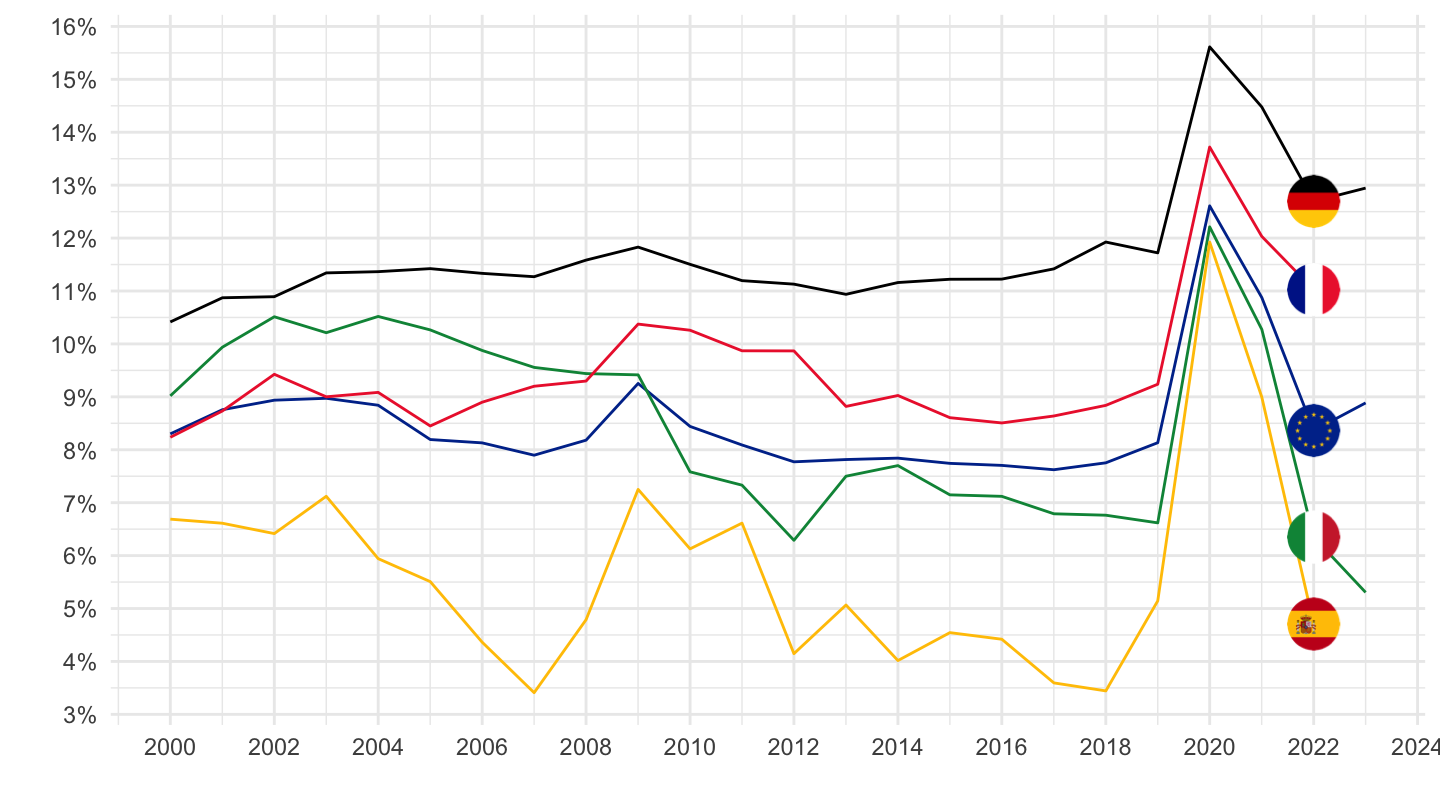
2015-
Code
nasa_10_nf_tr %>%
  filter(geo %in% c("FR", "DE", "IT", "ES", "EA20"),
         na_item == "B8G",
         direct == "PAID",
         unit == "CP_MNAC",
         sector == "S14_S15") %>%
  select(geo, time, values, sector) %>%
  left_join(gdp, by = c("geo", "time")) %>%
  mutate(values = values/gdp) %>%
  year_to_date %>%
  left_join(geo, by = "geo") %>%
  mutate(Geo = ifelse(geo == "EA20", "Europe", Geo)) %>%
  left_join(colors, by = c("Geo" = "country")) %>%
  filter(date >= as.Date("2015-01-01")) %>%
  ggplot + theme_minimal() + xlab("") + ylab("") +
  geom_line(aes(x = date, y = values, color = color)) +
  scale_color_identity() + add_5flags +
  scale_x_date(breaks = as.Date(paste0(seq(1940, 2100, 1), "-01-01")),
               labels = date_format("%Y")) +
  scale_y_continuous(breaks = 0.01*seq(0, 100, 1),
                labels = percent_format(a = 1))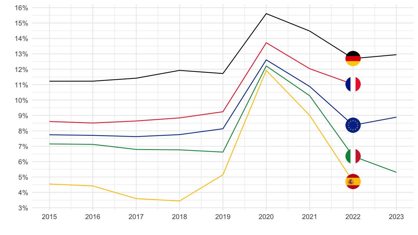
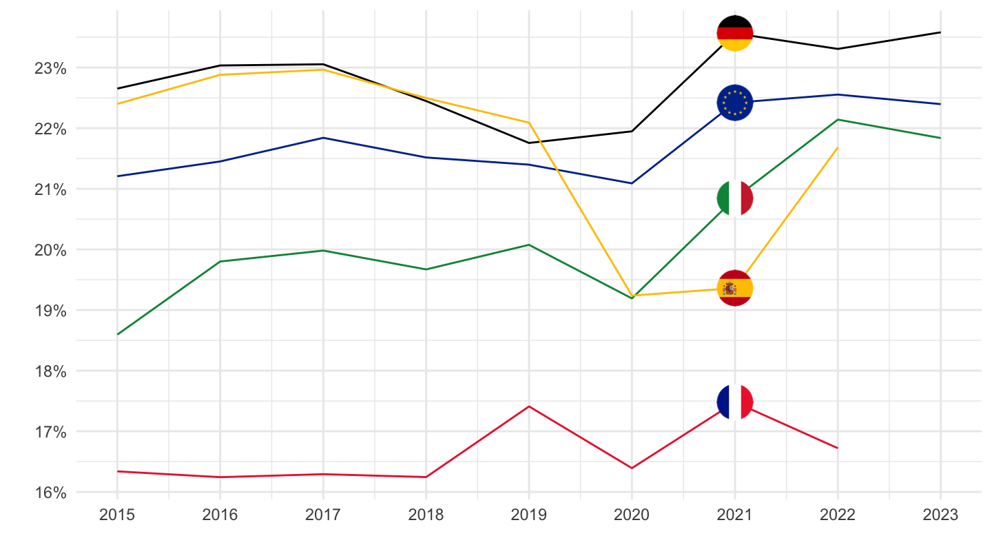
Operating surplus and mixed income, gross - B2A3G, S14_S15
All
Code
nasa_10_nf_tr %>%
  filter(geo %in% c("FR", "DE", "IT", "ES", "EA20"),
         na_item == "B2A3G",
         direct == "PAID",
         unit == "CP_MNAC",
         sector == "S14_S15") %>%
  select(geo, time, values, sector) %>%
  left_join(gdp, by = c("geo", "time")) %>%
  mutate(values = values/gdp) %>%
  year_to_date %>%
  left_join(geo, by = "geo") %>%
  mutate(Geo = ifelse(geo == "EA20", "Europe", Geo)) %>%
  left_join(colors, by = c("Geo" = "country")) %>%
  na.omit %>%
  ggplot + theme_minimal() + xlab("") + ylab("") +
  geom_line(aes(x = date, y = values, color = color)) +
  scale_color_identity() + add_5flags +
  scale_x_date(breaks = as.Date(paste0(seq(1940, 2100, 10), "-01-01")),
               labels = date_format("%Y")) +
  scale_y_continuous(breaks = 0.01*seq(0, 100, 1),
                labels = percent_format(a = 1))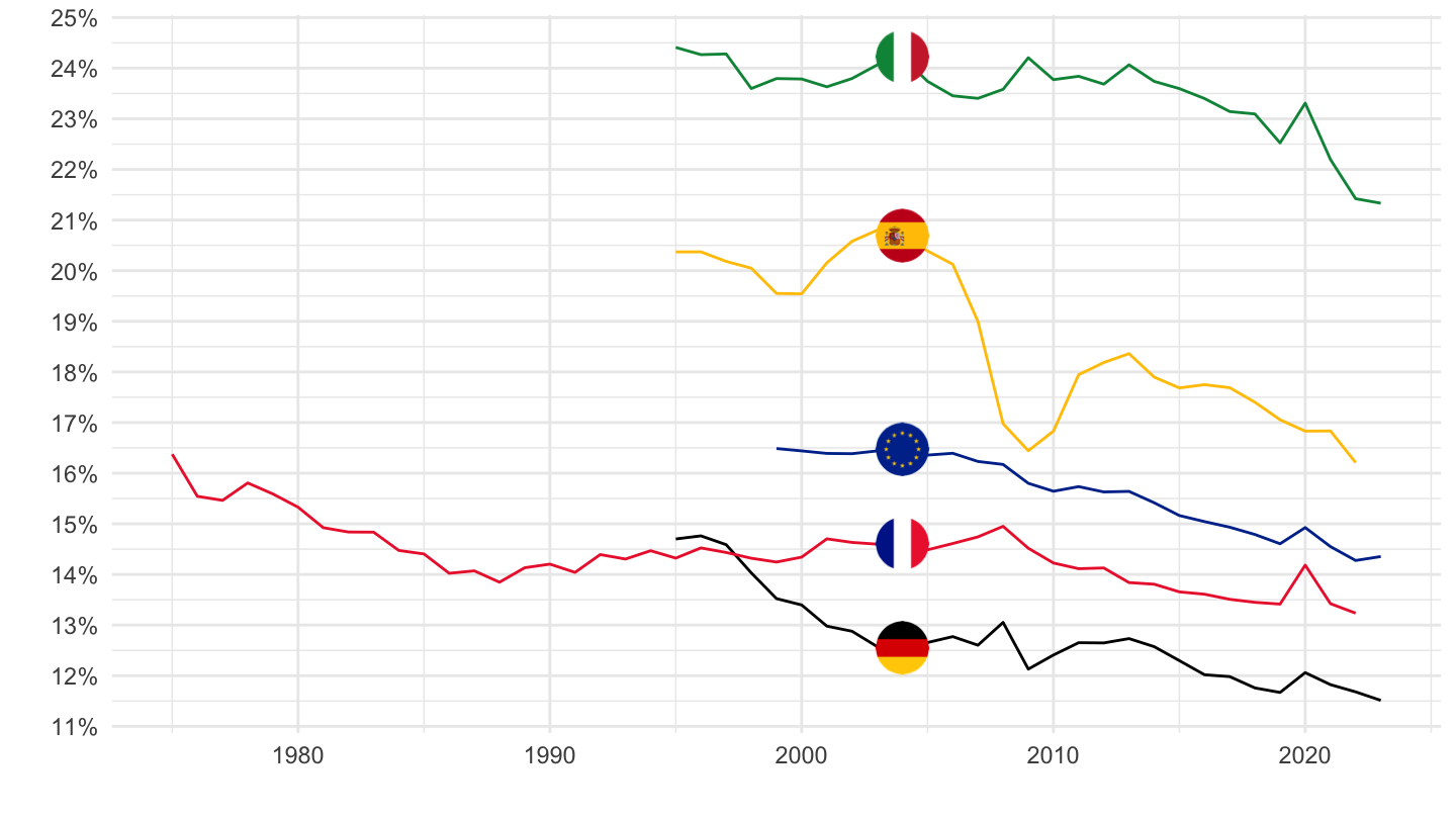
2000-
Code
nasa_10_nf_tr %>%
  filter(geo %in% c("FR", "DE", "IT", "ES", "EA20"),
         na_item == "B2A3G",
         direct == "PAID",
         unit == "CP_MNAC",
         sector == "S14_S15") %>%
  select(geo, time, values, sector) %>%
  left_join(gdp, by = c("geo", "time")) %>%
  mutate(values = values/gdp) %>%
  year_to_date %>%
  left_join(geo, by = "geo") %>%
  mutate(Geo = ifelse(geo == "EA20", "Europe", Geo)) %>%
  left_join(colors, by = c("Geo" = "country")) %>%
  filter(date >= as.Date("2000-01-01")) %>%
  ggplot + theme_minimal() + xlab("") + ylab("") +
  geom_line(aes(x = date, y = values, color = color)) +
  scale_color_identity() + add_5flags +
  scale_x_date(breaks = as.Date(paste0(seq(1940, 2100, 5), "-01-01")),
               labels = date_format("%Y")) +
  scale_y_continuous(breaks = 0.01*seq(0, 100, 1),
                labels = percent_format(a = 1))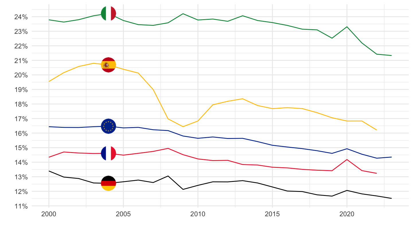
2015-
Code
nasa_10_nf_tr %>%
  filter(geo %in% c("FR", "DE", "IT", "ES", "EA20"),
         na_item == "B2A3G",
         direct == "PAID",
         unit == "CP_MNAC",
         sector == "S14_S15") %>%
  select(geo, time, values, sector) %>%
  left_join(gdp, by = c("geo", "time")) %>%
  mutate(values = values/gdp) %>%
  year_to_date %>%
  left_join(geo, by = "geo") %>%
  mutate(Geo = ifelse(geo == "EA20", "Europe", Geo)) %>%
  left_join(colors, by = c("Geo" = "country")) %>%
  filter(date >= as.Date("2015-01-01")) %>%
  ggplot + theme_minimal() + xlab("") + ylab("") +
  geom_line(aes(x = date, y = values, color = color)) +
  scale_color_identity() + add_5flags +
  scale_x_date(breaks = as.Date(paste0(seq(1940, 2100, 1), "-01-01")),
               labels = date_format("%Y")) +
  scale_y_continuous(breaks = 0.01*seq(0, 100, 1),
                labels = percent_format(a = 1))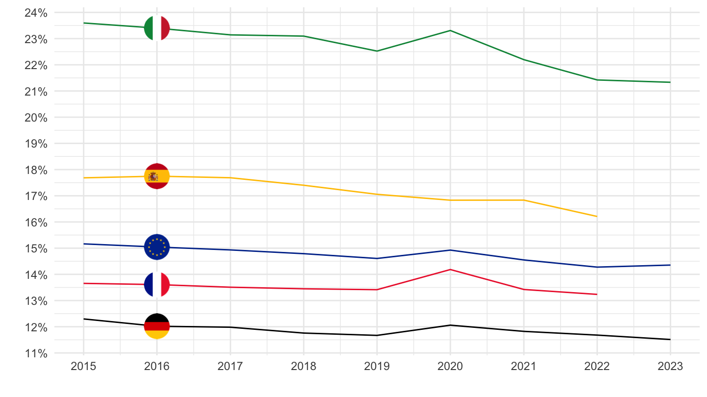
Operating surplus and mixed income, gross - B2A3G, S11
All
Code
nasa_10_nf_tr %>%
  filter(geo %in% c("FR", "DE", "IT", "ES", "EA20"),
         na_item == "B2A3G",
         direct == "PAID",
         unit == "CP_MNAC",
         sector == "S11") %>%
  select(geo, time, values, sector) %>%
  left_join(gdp, by = c("geo", "time")) %>%
  mutate(values = values/gdp) %>%
  year_to_date %>%
  left_join(geo, by = "geo") %>%
  mutate(Geo = ifelse(geo == "EA20", "Europe", Geo)) %>%
  left_join(colors, by = c("Geo" = "country")) %>%
  na.omit %>%
  ggplot + theme_minimal() + xlab("") + ylab("") +
  geom_line(aes(x = date, y = values, color = color)) +
  scale_color_identity() + add_5flags +
  scale_x_date(breaks = as.Date(paste0(seq(1940, 2100, 10), "-01-01")),
               labels = date_format("%Y")) +
  scale_y_continuous(breaks = 0.01*seq(0, 100, 1),
                labels = percent_format(a = 1))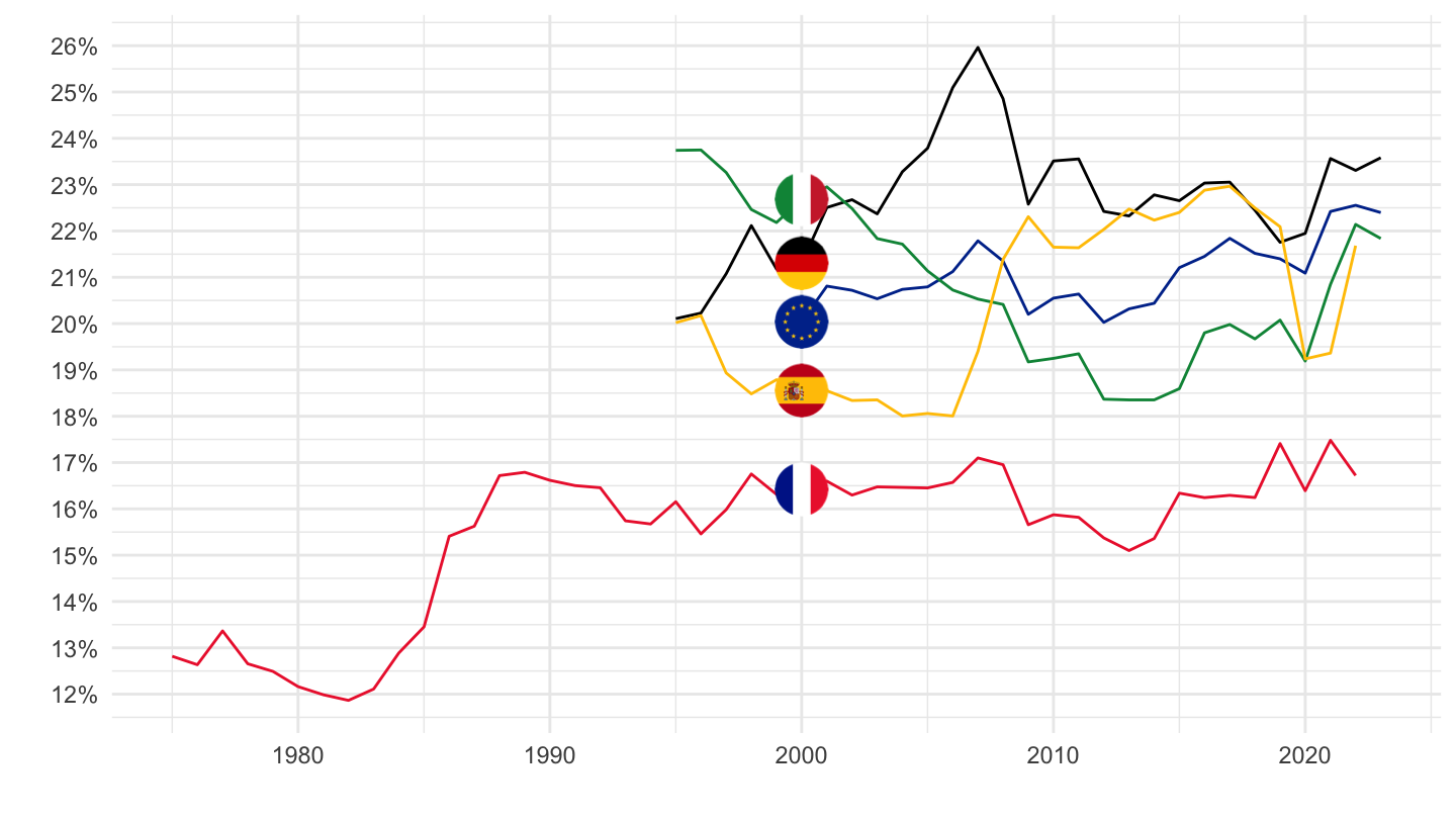
2000-
Code
nasa_10_nf_tr %>%
  filter(geo %in% c("FR", "DE", "IT", "ES", "EA20"),
         na_item == "B2A3G",
         direct == "PAID",
         unit == "CP_MNAC",
         sector == "S11") %>%
  select(geo, time, values, sector) %>%
  left_join(gdp, by = c("geo", "time")) %>%
  mutate(values = values/gdp) %>%
  year_to_date %>%
  left_join(geo, by = "geo") %>%
  mutate(Geo = ifelse(geo == "EA20", "Europe", Geo)) %>%
  left_join(colors, by = c("Geo" = "country")) %>%
  filter(date >= as.Date("2000-01-01")) %>%
  ggplot + theme_minimal() + xlab("") + ylab("") +
  geom_line(aes(x = date, y = values, color = color)) +
  scale_color_identity() + add_5flags +
  scale_x_date(breaks = as.Date(paste0(seq(1940, 2100, 5), "-01-01")),
               labels = date_format("%Y")) +
  scale_y_continuous(breaks = 0.01*seq(0, 100, 1),
                labels = percent_format(a = 1))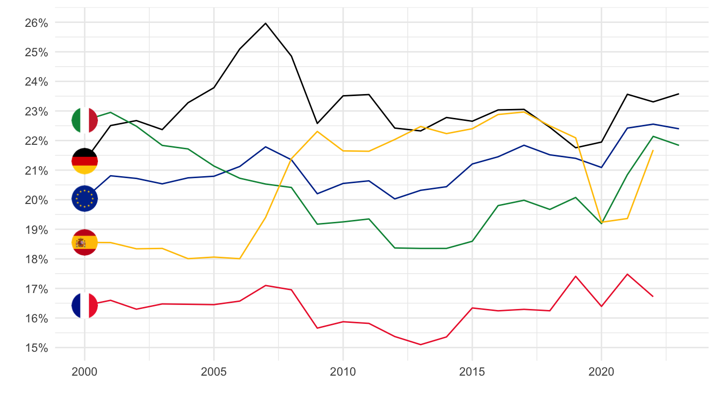
2015-
Code
nasa_10_nf_tr %>%
  filter(geo %in% c("FR", "DE", "IT", "ES", "EA20"),
         na_item == "B2A3G",
         direct == "PAID",
         unit == "CP_MNAC",
         sector == "S11") %>%
  select(geo, time, values, sector) %>%
  left_join(gdp, by = c("geo", "time")) %>%
  mutate(values = values/gdp) %>%
  year_to_date %>%
  left_join(geo, by = "geo") %>%
  mutate(Geo = ifelse(geo == "EA20", "Europe", Geo)) %>%
  left_join(colors, by = c("Geo" = "country")) %>%
  filter(date >= as.Date("2015-01-01")) %>%
  ggplot + theme_minimal() + xlab("") + ylab("") +
  geom_line(aes(x = date, y = values, color = color)) +
  scale_color_identity() + add_5flags +
  scale_x_date(breaks = as.Date(paste0(seq(1940, 2100, 1), "-01-01")),
               labels = date_format("%Y")) +
  scale_y_continuous(breaks = 0.01*seq(0, 100, 1),
                labels = percent_format(a = 1))