| source | dataset | Title | .html | .rData |
|---|---|---|---|---|
| eurostat | sts_inpr_m | Production in industry - monthly data | 2026-07-20 | 2026-07-20 |
Production in industry - monthly data
Data - Eurostat
Info
Data on industry
| source | dataset | Title | .html | .rData |
|---|---|---|---|---|
| eurostat | sts_inpr_m | Production in industry - monthly data | 2026-07-20 | 2026-07-20 |
| ec | INDUSTRY | Industry (sector data) | 2026-07-20 | 2026-07-20 |
| eurostat | ei_isin_m | Industry - monthly data - index (2015 = 100) (NACE Rev. 2) - ei_isin_m | 2026-07-20 | 2026-07-20 |
| eurostat | htec_trd_group4 | High-tech trade by high-tech group of products in million euro (from 2007, SITC Rev. 4) | 2026-07-20 | 2026-07-20 |
| eurostat | nama_10_a64 | National accounts aggregates by industry (up to NACE A*64) | 2026-07-17 | 2026-07-20 |
| eurostat | nama_10_a64_e | National accounts employment data by industry (up to NACE A*64) | 2026-07-20 | 2026-07-20 |
| eurostat | namq_10_a10_e | Employment A*10 industry breakdowns | 2026-07-20 | 2026-07-20 |
| eurostat | road_eqr_carmot | New registrations of passenger cars by type of motor energy and engine size - road_eqr_carmot | 2026-07-20 | 2026-07-20 |
| eurostat | sts_inpp_m | Producer prices in industry, total - monthly data | 2026-07-20 | 2026-07-20 |
| eurostat | sts_inppd_m | Producer prices in industry, domestic market - monthly data | 2026-07-20 | 2026-07-20 |
| eurostat | sts_intvnd_m | Turnover in industry, non domestic market - monthly data - sts_intvnd_m | 2026-03-24 | 2026-07-20 |
| fred | industry | Manufacturing, Industry | 2026-07-20 | 2026-07-20 |
| oecd | ALFS_EMP | Employment by activities and status (ALFS) | 2024-04-16 | 2025-05-24 |
| oecd | BERD_MA_SOF | Business enterprise R&D expenditure by main activity (focussed) and source of funds | 2024-04-16 | 2023-09-09 |
| oecd | GBARD_NABS2007 | Government budget allocations for R and D | 2024-04-16 | 2023-11-22 |
| oecd | MEI_REAL | Production and Sales (MEI) | 2024-05-12 | 2025-05-24 |
| oecd | MSTI_PUB | Main Science and Technology Indicators | 2024-09-15 | 2025-05-24 |
| oecd | SNA_TABLE4 | PPPs and exchange rates | 2024-09-15 | 2025-05-24 |
| wdi | NV.IND.EMPL.KD | Industry, value added per worker (constant 2010 USD) | 2024-01-06 | 2026-07-20 |
| wdi | NV.IND.MANF.CD | Manufacturing, value added (current USD) | 2026-07-20 | 2026-07-20 |
| wdi | NV.IND.MANF.ZS | Manufacturing, value added (% of GDP) | 2025-05-24 | 2026-07-20 |
| wdi | NV.IND.TOTL.KD | Industry (including construction), value added (constant 2015 USD) - NV.IND.TOTL.KD | 2024-01-06 | 2026-07-20 |
| wdi | NV.IND.TOTL.ZS | Industry, value added (including construction) (% of GDP) | 2025-05-24 | 2026-07-20 |
| wdi | SL.IND.EMPL.ZS | Employment in industry (% of total employment) | 2026-07-20 | 2026-07-20 |
| wdi | TX.VAL.MRCH.CD.WT | Merchandise exports (current USD) | 2024-01-06 | 2026-07-20 |
Last
Code
sts_inpr_m %>%
  group_by(time) %>%
  summarise(Nobs = n()) %>%
  arrange(desc(time)) %>%
  head(2) %>%
print_table_conditional()| time | Nobs |
|---|---|
| 2026M02 | 17080 |
| 2026M01 | 21107 |
nace_r2
Code
sts_inpr_m %>%
  left_join(nace_r2, by = "nace_r2") %>%
  group_by(nace_r2, Nace_r2) %>%
  summarise(Nobs = n()) %>%
  print_table_conditional()
s_adj
Code
sts_inpr_m %>%
  left_join(s_adj, by = "s_adj") %>%
  group_by(s_adj, S_adj) %>%
  summarise(Nobs = n()) %>%
  arrange(-Nobs) %>%
print_table_conditional()| s_adj | S_adj | Nobs |
|---|---|---|
| CA | Calendar adjusted data, not seasonally adjusted data | 6021272 |
| SCA | Seasonally and calendar adjusted data | 5888014 |
| NSA | Unadjusted data (i.e. neither seasonally adjusted nor calendar adjusted data) | 3169170 |
unit
Code
sts_inpr_m %>%
  left_join(unit, by = "unit") %>%
  group_by(unit, Unit) %>%
  summarise(Nobs = n()) %>%
  arrange(-Nobs) %>%
print_table_conditional()| unit | Unit | Nobs |
|---|---|---|
| I15 | Index, 2015=100 | 4316426 |
| I21 | Index, 2021=100 | 4223044 |
| I10 | Index, 2010=100 | 2920855 |
| PCH_PRE | Percentage change on previous period | 1821534 |
| PCH_SM | Percentage change compared to same period in previous year | 1796597 |
geo
Code
sts_inpr_m %>%
  left_join(geo, by = "geo") %>%
  group_by(geo, Geo) %>%
  summarise(Nobs = n()) %>%
  arrange(-Nobs) %>%
  mutate(Geo = ifelse(geo == "DE", "Germany", Geo)) %>%
  mutate(Flag = gsub(" ", "-", str_to_lower(Geo)),
         Flag = paste0('<img src="../../bib/flags/vsmall/', Flag, '.png" alt="Flag">')) %>%
  select(Flag, everything()) %>%
  {if (is_html_output()) datatable(., filter = 'top', rownames = F, escape = F) else .}
time
Code
sts_inpr_m %>%
  group_by(time) %>%
  summarise(Nobs = n()) %>%
  arrange(desc(time)) %>%
  print_table_conditional()
Last
Code
sts_inpr_m %>%
  filter(time == max(time), !is.na(values)) %>%
  print_table_conditional()
France VS EU
EU 2027
All
Code
sts_inpr_m %>%
  filter(nace_r2 == "C",
         unit == "I21",
         geo %in% c("FR", "EU27_2020"),
         s_adj == "SCA") %>%
  select(geo, time, values) %>%
  left_join(geo, by = "geo") %>%
  mutate(Geo = ifelse(geo == "DE", "Germany", Geo)) %>%
  mutate(Geo = ifelse(geo == "EU27_2020", "Europe", Geo)) %>%
  month_to_date %>%
  group_by(geo) %>%
  arrange(date) %>%
  mutate(values = 100*values/values[1]) %>%
  #filter(date >= as.Date("2000-01-01")) %>%
  left_join(colors, by = c("Geo" = "country")) %>%
  ggplot() + ylab("Industrial Production") + xlab("") + theme_minimal() +
  geom_line(aes(x = date, y = values, color = color)) +
  scale_color_identity() +
  scale_x_date(breaks = seq(1920, 2100, 2) %>% paste0("-01-01") %>% as.Date,
               labels = date_format("%Y")) +
  add_2flags +
  scale_y_log10(breaks = seq(-60, 300, 10))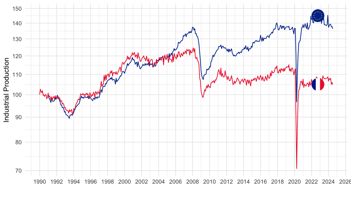
1992-
Code
sts_inpr_m %>%
  filter(nace_r2 == "C",
         unit == "I21",
         geo %in% c("FR", "EU27_2020"),
         s_adj == "SCA") %>%
  select(geo, time, values) %>%
  group_by(geo) %>%
  mutate(values = 100*values/values[time == "1992M01"]) %>%
  left_join(geo, by = "geo") %>%
  mutate(Geo = ifelse(geo == "DE", "Germany", Geo)) %>%
  mutate(Geo = ifelse(geo == "EU27_2020", "Europe", Geo)) %>%
  month_to_date %>%
  filter(date >= as.Date("1992-01-01")) %>%
  left_join(colors, by = c("Geo" = "country")) %>%
  ggplot() + ylab("Industrial Production") + xlab("") + theme_minimal() +
  geom_line(aes(x = date, y = values, color = color)) +
  scale_color_identity() +
  scale_x_date(breaks = seq(1920, 2100, 2) %>% paste0("-01-01") %>% as.Date,
               labels = date_format("%Y")) +
  add_2flags +
  scale_y_log10(breaks = seq(-60, 300, 10))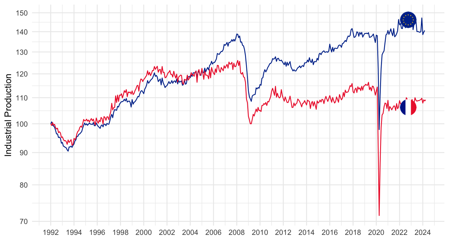
2000-
Code
sts_inpr_m %>%
  filter(nace_r2 == "C",
         unit == "I21",
         geo %in% c("FR", "EU27_2020"),
         s_adj == "SCA") %>%
  select(geo, time, values) %>%
  group_by(geo) %>%
  mutate(values = 100*values/values[time == "2000M01"]) %>%
  left_join(geo, by = "geo") %>%
  mutate(Geo = ifelse(geo == "DE", "Germany", Geo)) %>%
  mutate(Geo = ifelse(geo == "EU27_2020", "Europe", Geo)) %>%
  month_to_date %>%
  filter(date >= as.Date("2000-01-01")) %>%
  left_join(colors, by = c("Geo" = "country")) %>%
  ggplot() + ylab("Industrial Production") + xlab("") + theme_minimal() +
  geom_line(aes(x = date, y = values, color = color)) +
  scale_color_identity() +
  scale_x_date(breaks = seq(1920, 2100, 2) %>% paste0("-01-01") %>% as.Date,
               labels = date_format("%Y")) +
  add_2flags +
  scale_y_log10(breaks = seq(-60, 300, 10))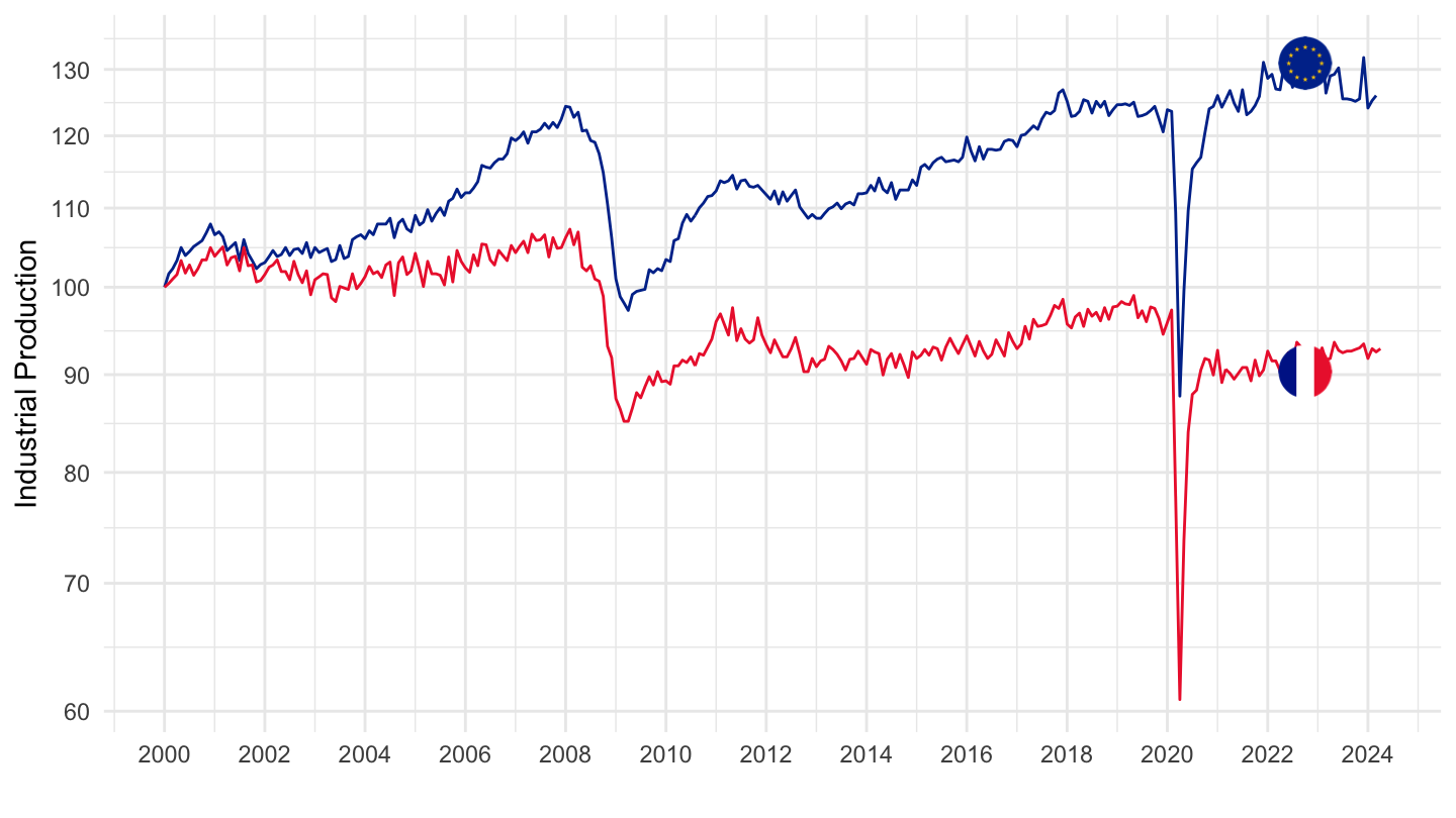
Eurozone
2000-
Code
sts_inpr_m %>%
  filter(nace_r2 == "C",
         unit == "I21",
         geo %in% c("FR", "EA20"),
         s_adj == "SCA") %>%
  select(geo, time, values) %>%
  group_by(geo) %>%
  mutate(values = 100*values/values[time == "2020M02"]) %>%
  left_join(geo, by = "geo") %>%
  mutate(Geo = ifelse(geo == "DE", "Germany", Geo)) %>%
  mutate(Geo = ifelse(geo == "EA20", "Europe", Geo)) %>%
  month_to_date %>%
  filter(date >= as.Date("2000-01-01")) %>%
  left_join(colors, by = c("Geo" = "country")) %>%
  ggplot() + ylab("Industrial Production") + xlab("") + theme_minimal() +
  geom_line(aes(x = date, y = values, color = color)) +
  scale_color_identity() +
  scale_x_date(breaks = seq(1920, 2100, 2) %>% paste0("-01-01") %>% as.Date,
               labels = date_format("%Y")) +
  add_2flags +
  scale_y_log10(breaks = seq(-60, 300, 10))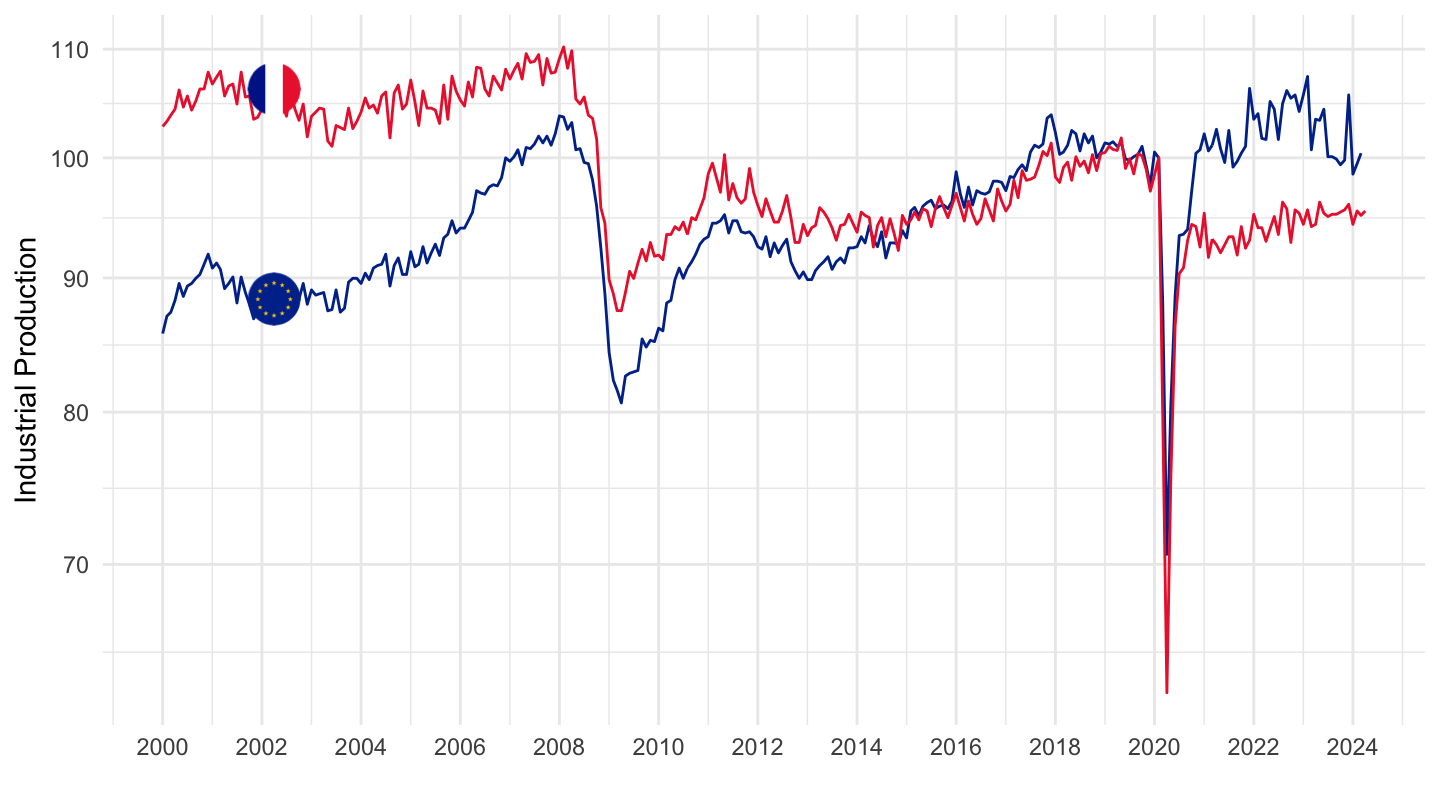
Germany
Index, Change
Code
sts_inpr_m %>%
  filter(geo == "DE",
         s_adj == "SCA",

         time %in% c("2022M08", "2022M07", "2022M03")) %>%
  select_if(~ n_distinct(.) > 1) %>%
  spread(time, values) %>%
  left_join(nace_r2, by = "nace_r2") %>%
  select(nace_r2, Nace_r2, everything()) %>%
  print_table_conditional()
Index
Code
sts_inpr_m %>%
  filter(geo == "DE",
         s_adj == "SCA",
         unit == "I21",
         time %in% c("2022M08", "2022M07", "2022M03")) %>%
  select_if(~ n_distinct(.) > 1) %>%
  spread(time, values) %>%
  left_join(nace_r2, by = "nace_r2") %>%
  select(nace_r2, Nace_r2, everything()) %>%
  print_table_conditional()
PCH_PRE - Change
Code
sts_inpr_m %>%
  filter(geo == "DE",
         #s_adj == "SCA",
         unit == "PCH_SM",
         time %in% c("2022M12", "2022M11", "2022M08", "2022M05","2022M03")) %>%
  select_if(~ n_distinct(.) > 1) %>%
  spread(time, values) %>%
  left_join(nace_r2, by = "nace_r2") %>%
  select(nace_r2, Nace_r2, everything()) %>%
  arrange(`2022M11`) %>%
  print_table_conditional()
Fertilizers, Chemical industry
All
Code
sts_inpr_m %>%
  filter(geo == "DE",
         s_adj == "SCA",
         unit == "I21",
         nace_r2 %in% c("C2015", "C20_C21", "C20", "C2442")) %>%
  month_to_date %>%
  left_join(nace_r2, by = "nace_r2") %>%
  mutate(Nace_r2 = gsub("Manufacture", "Manuf.", Nace_r2)) %>%
  ggplot + geom_line(aes(x = date, y = values, color = Nace_r2)) +
  xlab("") + ylab("") + theme_minimal() +
  theme(legend.position = c(0.5, 0.25),
        legend.title = element_blank()) +
  scale_x_date(breaks = "5 years",
               labels = date_format("%Y")) +
  scale_y_log10(breaks = seq(60, 120, 10))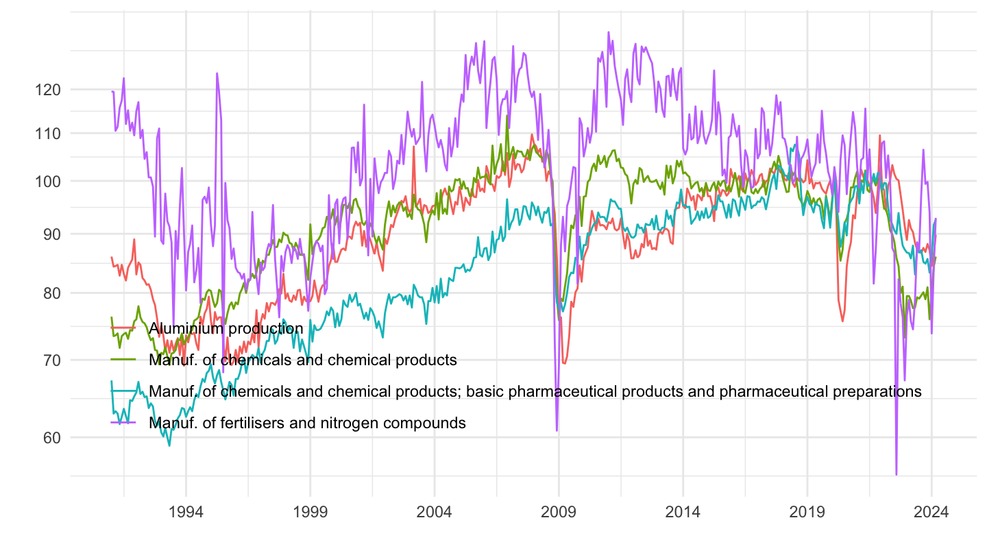
1995-
Code
sts_inpr_m %>%
  filter(geo == "DE",
         s_adj == "SCA",
         unit == "I21",
         nace_r2 %in% c("C2015", "C20_C21", "C20", "C2442")) %>%
  month_to_date %>%
  filter(date >= as.Date("1995-01-01")) %>%
  left_join(nace_r2, by = "nace_r2") %>%
  mutate(Nace_r2 = gsub("Manufacture", "Manuf.", Nace_r2)) %>%
  ggplot + geom_line(aes(x = date, y = values, color = Nace_r2)) +
  xlab("") + ylab("") + theme_minimal() +
  theme(legend.position = c(0.5, 0.25),
        legend.title = element_blank()) +
  scale_x_date(breaks = "5 years",
               labels = date_format("%Y")) +
  scale_y_log10(breaks = seq(60, 120, 10))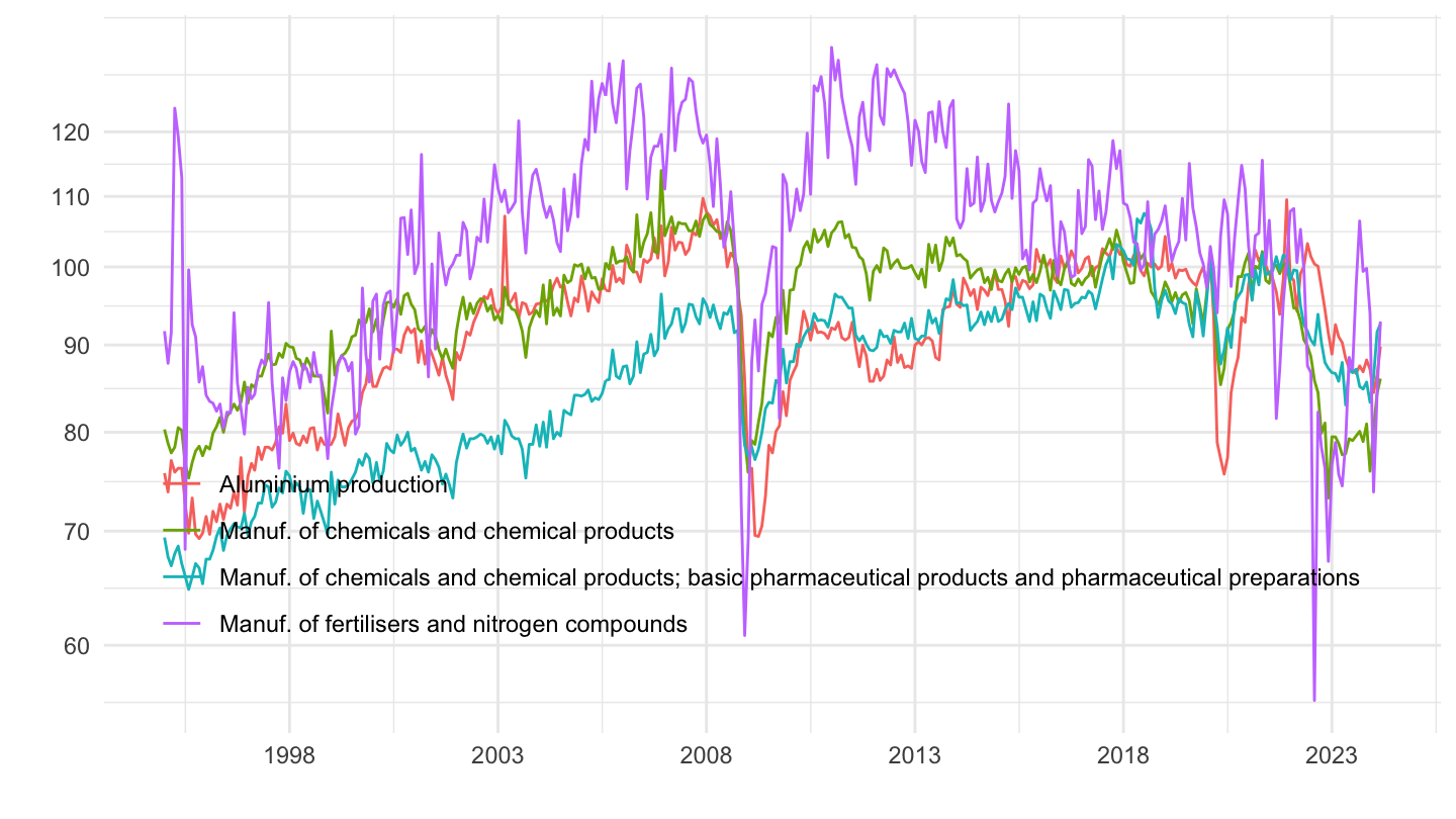
2010-
Code
sts_inpr_m %>%
  filter(geo == "DE",
         s_adj == "SCA",
         unit == "I21",
         nace_r2 %in% c("C2015", "C20_C21", "C20", "C2442")) %>%
  month_to_date %>%
  filter(date >= as.Date("2010-01-01")) %>%
  left_join(nace_r2, by = "nace_r2") %>%
  mutate(Nace_r2 = gsub("Manufacture", "Manuf.", Nace_r2)) %>%
  ggplot + geom_line(aes(x = date, y = values, color = Nace_r2)) +
  xlab("") + ylab("") + theme_minimal() +
  theme(legend.position = c(0.5, 0.25),
        legend.title = element_blank()) +
  scale_x_date(breaks = "1 year",
               labels = date_format("%Y")) +
  scale_y_log10(breaks = seq(60, 120, 10))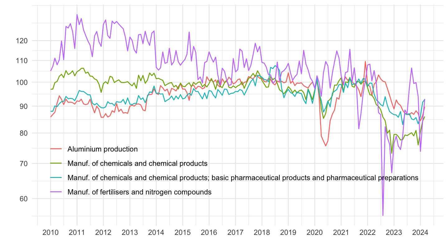
2017-
Code
sts_inpr_m %>%
  filter(geo == "DE",
         s_adj == "SCA",
         unit == "I21",
         nace_r2 %in% c("C2015", "C20_C21", "C20", "C2442")) %>%
  month_to_date %>%
  filter(date >= as.Date("2017-01-01")) %>%
  left_join(nace_r2, by = "nace_r2") %>%
  mutate(Nace_r2 = gsub("Manufacture", "Manuf.", Nace_r2)) %>%
  ggplot + geom_line(aes(x = date, y = values, color = Nace_r2)) +
  xlab("") + ylab("") + theme_minimal() +
  theme(legend.position = c(0.5, 0.25),
        legend.title = element_blank()) +
  scale_x_date(breaks = "1 year",
               labels = date_format("%Y")) +
  scale_y_log10(breaks = seq(40, 120, 10))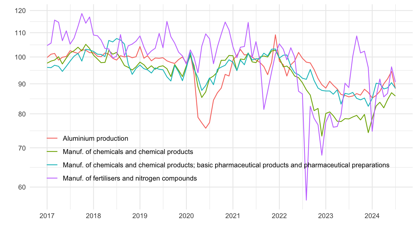
2020-
Code
sts_inpr_m %>%
  filter(geo == "DE",
         s_adj == "SCA",
         unit == "I21",
         nace_r2 %in% c("C2015", "C20_C21", "C20", "C2442")) %>%
  month_to_date %>%
  filter(date >= as.Date("2020-01-01")) %>%
  left_join(nace_r2, by = "nace_r2") %>%
  mutate(Nace_r2 = gsub("Manufacture", "Manuf.", Nace_r2)) %>%
  ggplot + geom_line(aes(x = date, y = values, color = Nace_r2)) +
  xlab("") + ylab("") + theme_minimal() +
  theme(legend.position = c(0.5, 0.25),
        axis.text.x = element_text(angle = 45, vjust = 1, hjust = 1),
        legend.title = element_blank()) +
  scale_x_date(breaks = "3 months",
               labels = date_format("%b %y")) +
  scale_y_log10(breaks = seq(40, 120, 5))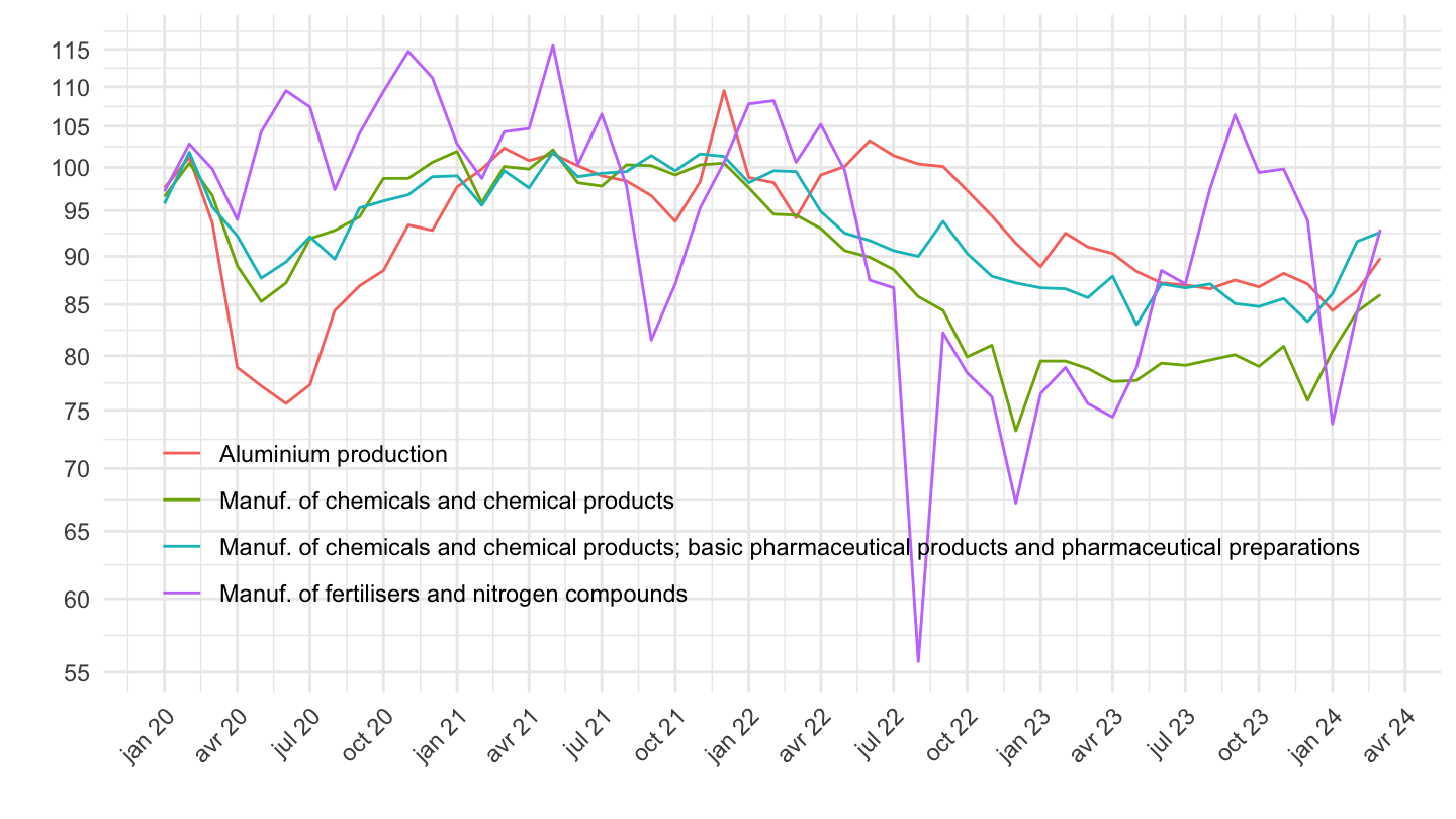
France, Germany, Italy, Greece, Europe
1995-
Code
sts_inpr_m %>%
  filter(nace_r2 == "C",
         unit == "I21",
         geo %in% c("FR", "DE", "IT", "EA20", "EL"),
         s_adj == "SCA") %>%
  select(geo, time, values) %>%
  group_by(geo) %>%
  month_to_date %>%
  filter(date >= as.Date("1995-01-01")) %>%
  arrange(date) %>%
  mutate(values = 100*values/values[1]) %>%
  left_join(geo, by = "geo") %>%
  mutate(Geo = ifelse(geo == "DE", "Germany", Geo)) %>%
  mutate(Geo = ifelse(geo == "EA20", "Europe", Geo)) %>%
  left_join(colors, by = c("Geo" = "country")) %>%
  ggplot() + ylab("Industrial Production") + xlab("") + theme_minimal() +
  geom_line(aes(x = date, y = values, color = color)) +
  scale_color_identity() +
  scale_x_date(breaks = seq(1920, 2100, 2) %>% paste0("-01-01") %>% as.Date,
               labels = date_format("%Y")) +
  add_5flags +
  scale_y_log10(breaks = seq(-60, 300, 10))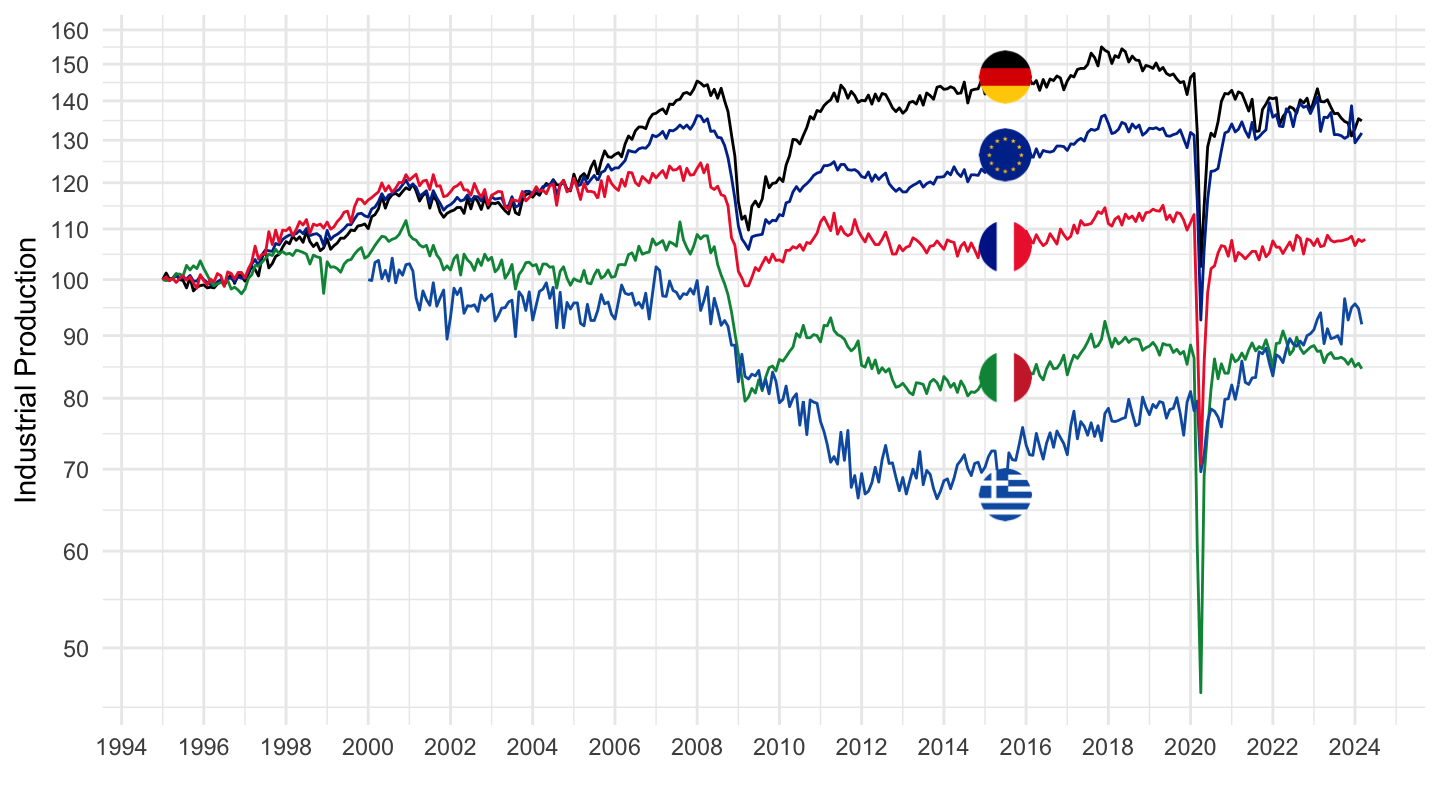
2000-
Code
sts_inpr_m %>%
  filter(nace_r2 == "C",
         unit == "I21",
         geo %in% c("FR", "DE", "IT", "EA20", "EL"),
         s_adj == "SCA") %>%
  select(geo, time, values) %>%
  group_by(geo) %>%
  month_to_date %>%
  filter(date >= as.Date("2000-01-01")) %>%
  arrange(date) %>%
  mutate(values = 100*values/values[1]) %>%
  left_join(geo, by = "geo") %>%
  mutate(Geo = ifelse(geo == "DE", "Germany", Geo)) %>%
  mutate(Geo = ifelse(geo == "EA20", "Europe", Geo)) %>%
  left_join(colors, by = c("Geo" = "country")) %>%
  ggplot() + ylab("Industrial Production") + xlab("") + theme_minimal() +
  geom_line(aes(x = date, y = values, color = color)) +
  scale_color_identity() +
  scale_x_date(breaks = seq(1920, 2100, 2) %>% paste0("-01-01") %>% as.Date,
               labels = date_format("%Y")) +
  add_5flags +
  scale_y_log10(breaks = seq(-60, 300, 10))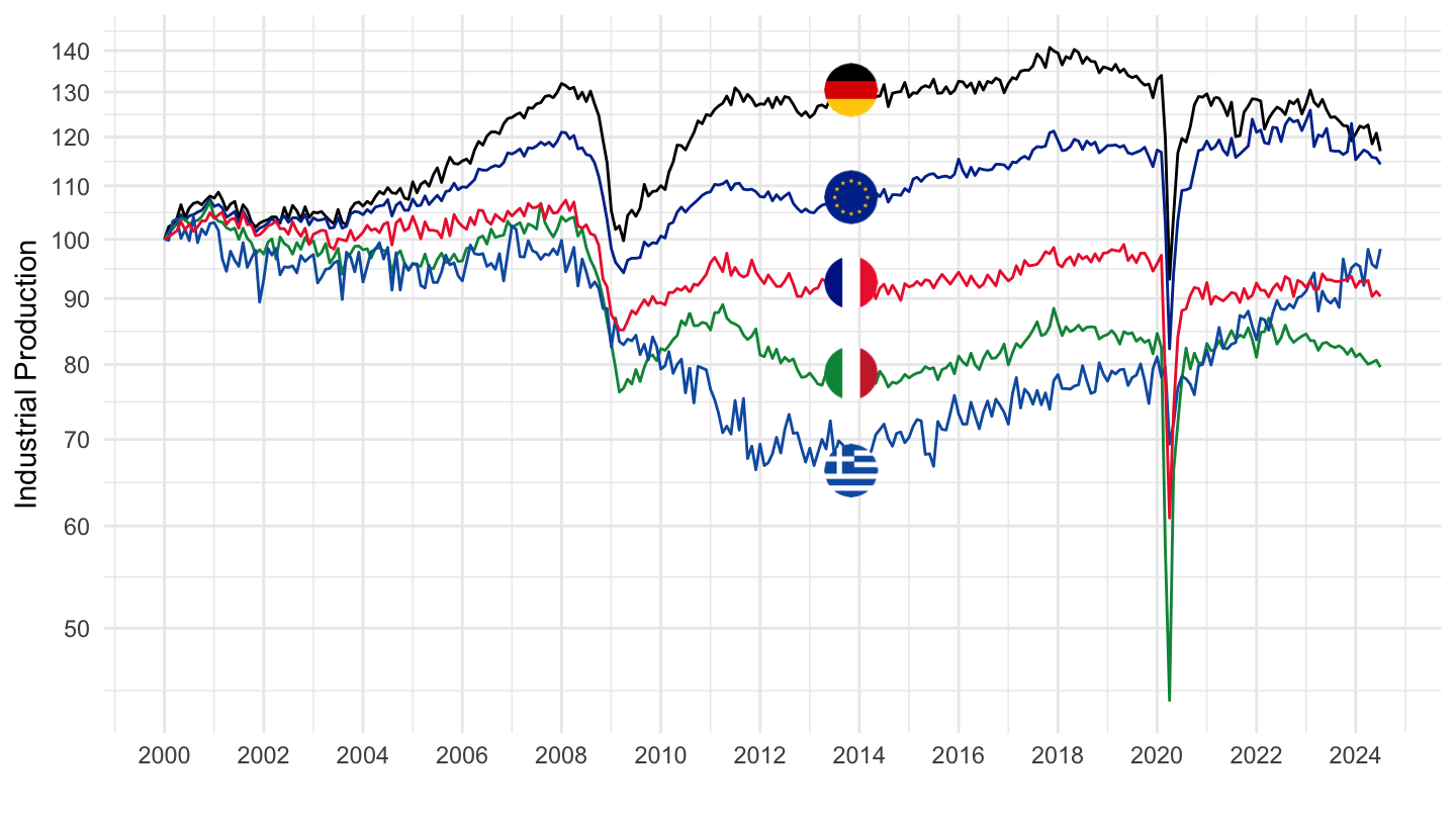
2008-
Code
sts_inpr_m %>%
  filter(nace_r2 == "C",
         unit == "I21",
         geo %in% c("FR", "DE", "IT", "EA20", "EL"),
         s_adj == "SCA") %>%
  select(geo, time, values) %>%
  group_by(geo) %>%
  month_to_date %>%
  filter(date >= as.Date("2008-01-01")) %>%
  arrange(date) %>%
  mutate(values = 100*values/values[1]) %>%
  left_join(geo, by = "geo") %>%
  mutate(Geo = ifelse(geo == "DE", "Germany", Geo)) %>%
  mutate(Geo = ifelse(geo == "EA20", "Europe", Geo)) %>%
  left_join(colors, by = c("Geo" = "country")) %>%
  ggplot() + ylab("Industrial Production") + xlab("") + theme_minimal() +
  geom_line(aes(x = date, y = values, color = color)) +
  scale_color_identity() +
  scale_x_date(breaks = seq(1920, 2100, 2) %>% paste0("-01-01") %>% as.Date,
               labels = date_format("%Y")) +
  add_5flags +
  scale_y_log10(breaks = seq(-60, 300, 10))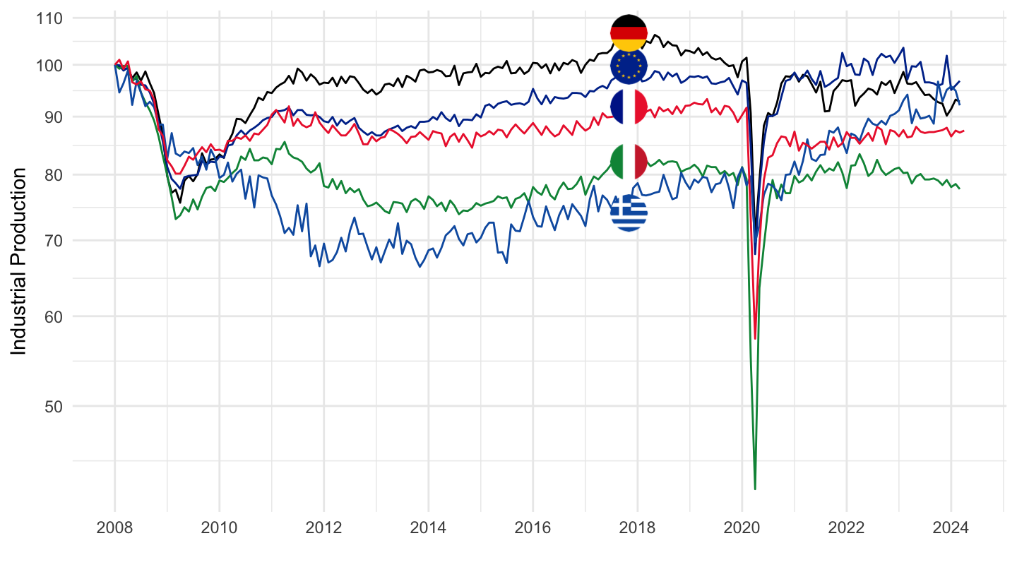
France, Germany, Italy
C20 - Manufacture of chemicals and chemical products
All
Code
sts_inpr_m %>%
  filter(nace_r2 == "C20",
         unit == "I21",
         geo %in% c("FR", "DE", "IT", "EA20"),
         s_adj == "SCA") %>%
  select(geo, time, values) %>%
  group_by(geo) %>%
  mutate(values = 100*values/values[time == "2010M01"]) %>%
  left_join(geo, by = "geo") %>%
  mutate(Geo = ifelse(geo == "DE", "Germany", Geo)) %>%
  mutate(Geo = ifelse(geo == "EA20", "Europe", Geo)) %>%
  month_to_date %>%
  left_join(colors, by = c("Geo" = "country")) %>%
  ggplot() + ylab("Industrial Production") + xlab("") + theme_minimal() +
  geom_line(aes(x = date, y = values, color = color)) +
  scale_color_identity() + add_4flags +
  scale_x_date(breaks = seq(1920, 2100, 5) %>% paste0("-01-01") %>% as.Date,
               labels = date_format("%Y")) +
  theme(legend.position = "none") +
  scale_y_log10(breaks = seq(-60, 300, 10))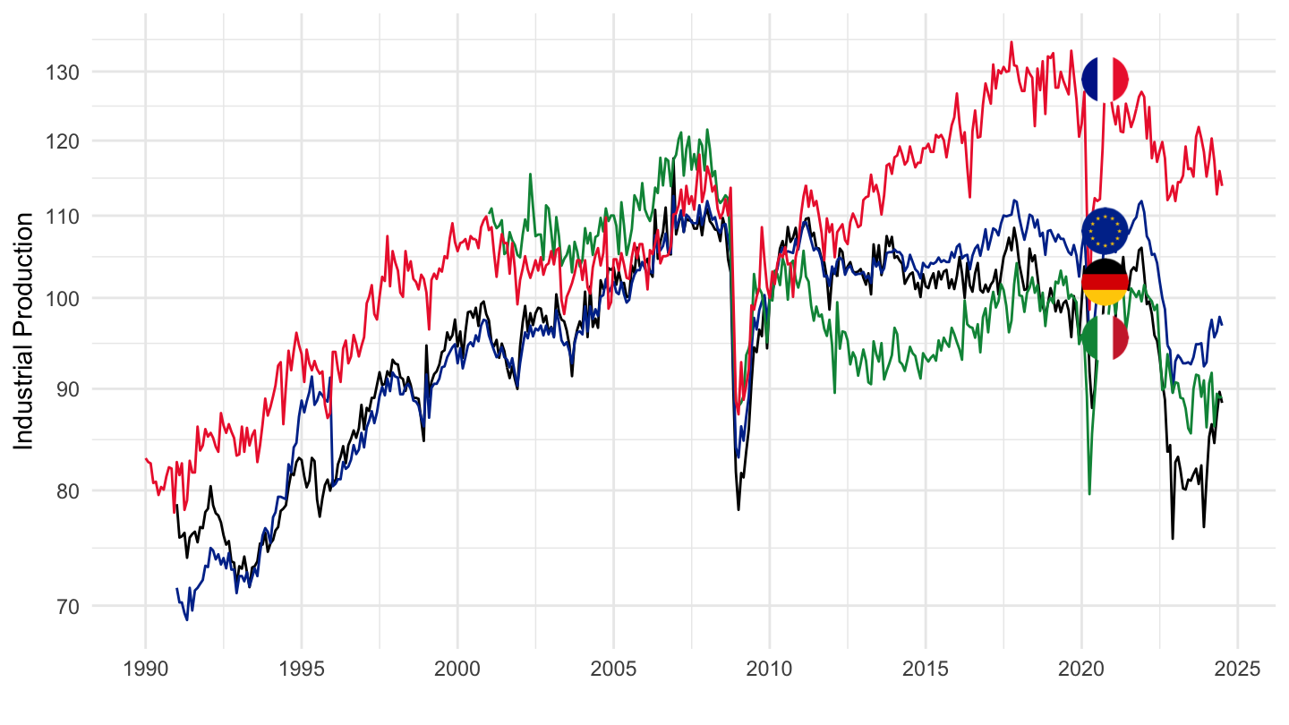
1992-
Code
sts_inpr_m %>%
  filter(nace_r2 == "C20",
         unit == "I21",
         geo %in% c("FR", "DE", "IT", "EA20"),
         s_adj == "SCA") %>%
  select(geo, time, values) %>%
  group_by(geo) %>%
  mutate(values = 100*values/values[time == "2001M01"]) %>%
  left_join(geo, by = "geo") %>%
  mutate(Geo = ifelse(geo == "DE", "Germany", Geo)) %>%
  mutate(Geo = ifelse(geo == "EA20", "Europe", Geo)) %>%
  month_to_date %>%
  filter(date >= as.Date("1992-01-01")) %>%
  left_join(colors, by = c("Geo" = "country")) %>%
  ggplot() + ylab("Industrial Production") + xlab("") + theme_minimal() +
  geom_line(aes(x = date, y = values, color = color)) +
  scale_color_identity() + add_4flags +
  scale_x_date(breaks = seq(1920, 2100, 2) %>% paste0("-01-01") %>% as.Date,
               labels = date_format("%Y")) +
  theme(legend.position = "none") +
  scale_y_log10(breaks = seq(-60, 300, 10))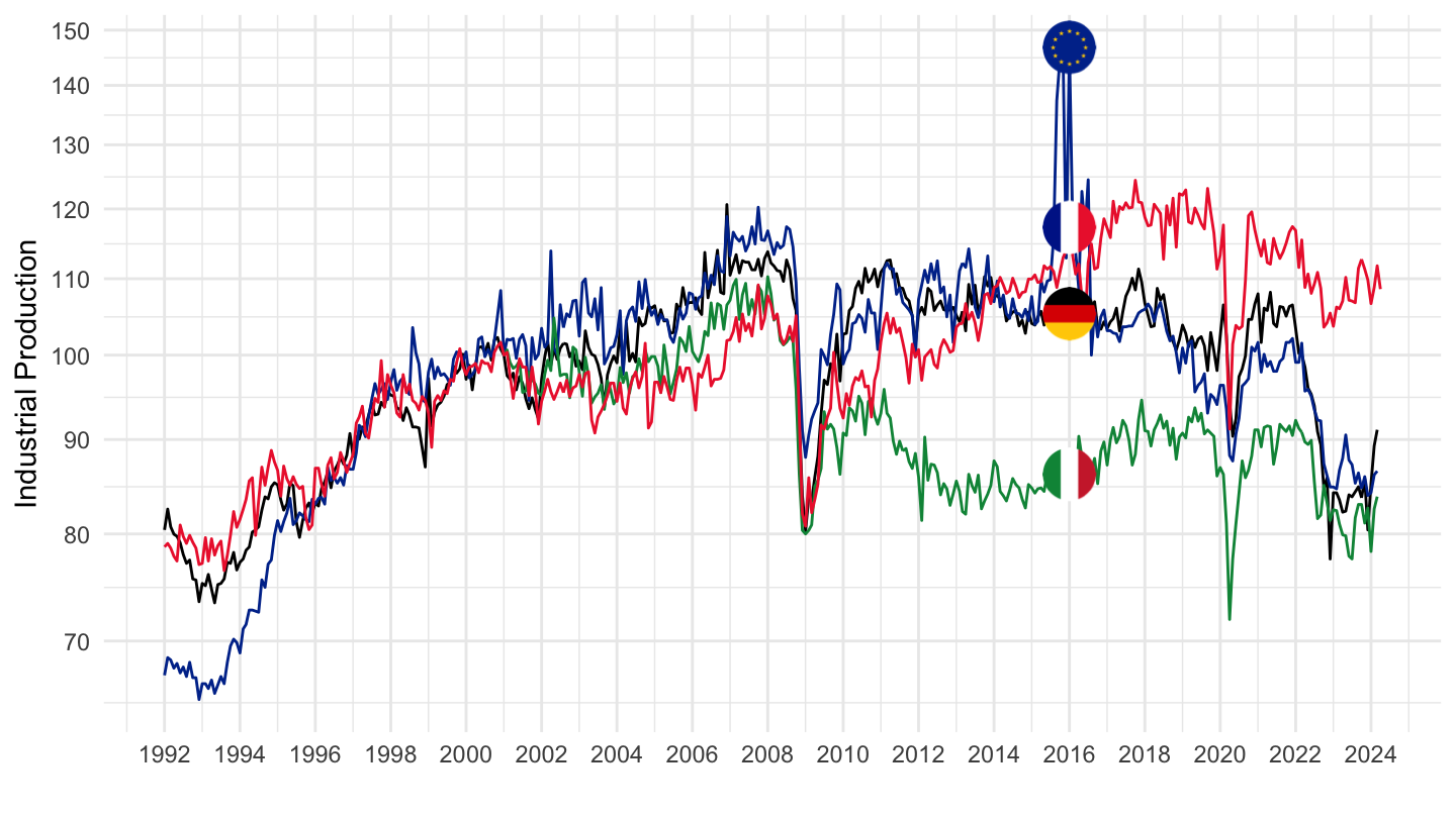
2000-
Code
sts_inpr_m %>%
  filter(nace_r2 == "C20",
         unit == "I21",
         geo %in% c("FR", "DE", "IT", "EA20"),
         s_adj == "SCA") %>%
  select(geo, time, values) %>%
  group_by(geo) %>%
  mutate(values = 100*values/values[time == "2001M01"]) %>%
  left_join(geo, by = "geo") %>%
  mutate(Geo = ifelse(geo == "DE", "Germany", Geo)) %>%
  mutate(Geo = ifelse(geo == "EA20", "Europe", Geo)) %>%
  month_to_date %>%
  filter(date >= as.Date("2000-01-01")) %>%
  left_join(colors, by = c("Geo" = "country")) %>%
  ggplot() + ylab("Industrial Production\nManufacture of fertilisers and nitrogen compounds") + xlab("") +
  geom_line(aes(x = date, y = values, color = color)) +
  scale_color_identity() + add_4flags + theme_minimal() +
  scale_x_date(breaks = seq(1920, 2100, 2) %>% paste0("-01-01") %>% as.Date,
               labels = date_format("%Y")) +
  scale_y_log10(breaks = seq(-60, 300, 10))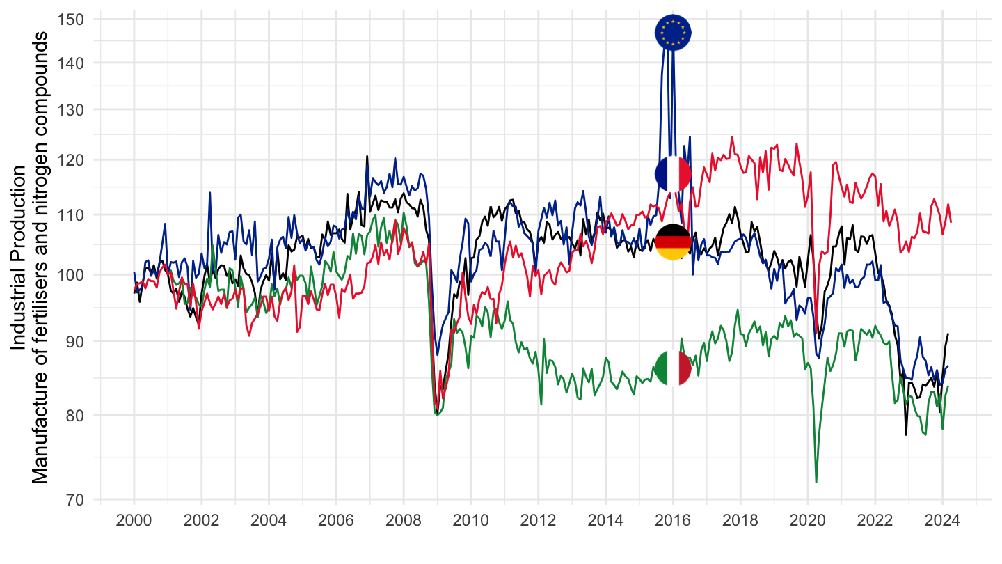
2019-
Code
sts_inpr_m %>%
  filter(nace_r2 == "C20",
         unit == "I21",
         geo %in% c("FR", "DE", "IT", "EA20"),
         s_adj == "SCA") %>%
  select(geo, time, values) %>%
  group_by(geo) %>%
  mutate(values = 100*values/values[time == "2019M01"]) %>%
  left_join(geo, by = "geo") %>%
  mutate(Geo = ifelse(geo == "DE", "Germany", Geo)) %>%
  mutate(Geo = ifelse(geo == "EA20", "Europe", Geo)) %>%
  month_to_date %>%
  filter(date >= as.Date("2019-01-01")) %>%
  left_join(colors, by = c("Geo" = "country")) %>%
  ggplot() + ylab("Industrial Production\nManufacture of fertilisers and nitrogen compounds") + xlab("") +
  geom_line(aes(x = date, y = values, color = color)) +
  scale_color_identity() + add_4flags + theme_minimal() +
  scale_x_date(breaks = "3 months",
               labels = date_format("%b %y")) +
  add_4flags +
  theme(legend.position = "none",
        axis.text.x = element_text(angle = 45, vjust = 1, hjust = 1)) +
  scale_y_log10(breaks = seq(-60, 300, 5))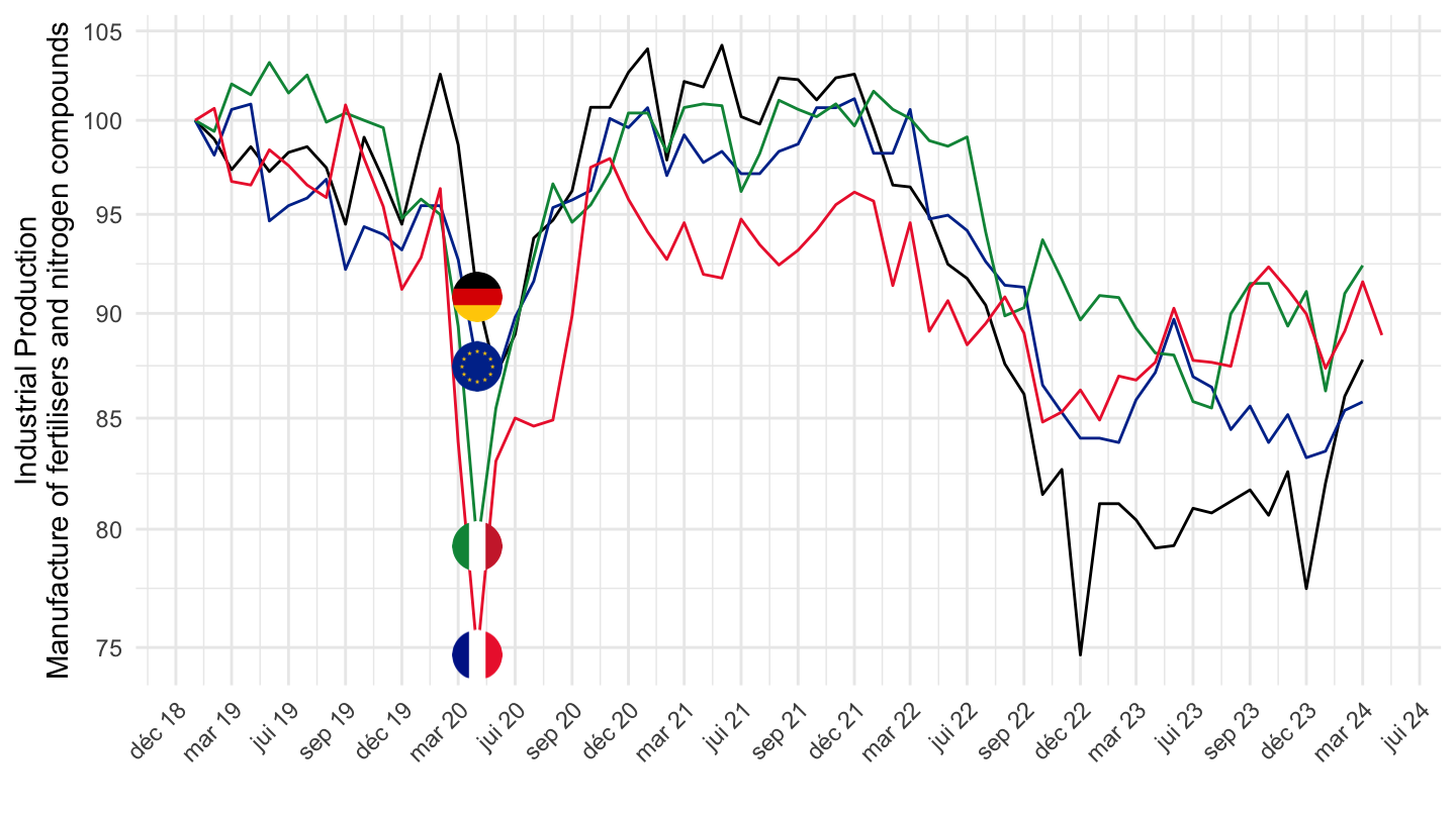
2020-
Code
sts_inpr_m %>%
  filter(nace_r2 == "C20",
         unit == "I21",
         geo %in% c("FR", "DE", "IT", "EA20"),
         s_adj == "SCA") %>%
  select(geo, time, values) %>%
  group_by(geo) %>%
  mutate(values = 100*values/values[time == "2020M01"]) %>%
  left_join(geo, by = "geo") %>%
  mutate(Geo = ifelse(geo == "DE", "Germany", Geo)) %>%
  mutate(Geo = ifelse(geo == "EA20", "Europe", Geo)) %>%
  month_to_date %>%
  filter(date >= as.Date("2020-01-01")) %>%
  left_join(colors, by = c("Geo" = "country")) %>%
  ggplot() + ylab("Industrial Production\nManufacture of fertilisers and nitrogen compounds") + xlab("") +
  geom_line(aes(x = date, y = values, color = color)) +
  scale_color_identity() + add_4flags + theme_minimal() +
  theme(legend.position = "none",
        axis.text.x = element_text(angle = 45, vjust = 1, hjust = 1)) +
  scale_x_date(breaks = "2 months",
               labels = date_format("%b %y")) +
  scale_y_log10(breaks = seq(-60, 300, 5))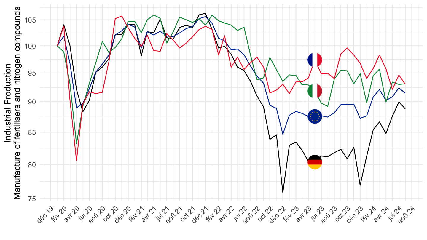
2021-
Code
sts_inpr_m %>%
  filter(nace_r2 == "C20",
         unit == "I21",
         geo %in% c("FR", "DE", "IT", "EA20"),
         s_adj == "SCA") %>%
  select(geo, time, values) %>%
  group_by(geo) %>%
  mutate(values = 100*values/values[time == "2021M01"]) %>%
  left_join(geo, by = "geo") %>%
  mutate(Geo = ifelse(geo == "DE", "Germany", Geo)) %>%
  mutate(Geo = ifelse(geo == "EA20", "Europe", Geo)) %>%
  month_to_date %>%
  filter(date >= as.Date("2021-01-01")) %>%
  left_join(colors, by = c("Geo" = "country")) %>%
  ggplot() + ylab("Industrial Production\nManufacture of chemicals and chemical products") + xlab("") +
  geom_line(aes(x = date, y = values, color = color)) +
  scale_color_identity() + add_4flags + theme_minimal() +
  theme(legend.position = "none",
        axis.text.x = element_text(angle = 45, vjust = 1, hjust = 1)) +
  scale_x_date(breaks = "2 months",
               labels = date_format("%b %y")) +
  scale_y_log10(breaks = seq(-60, 300, 5))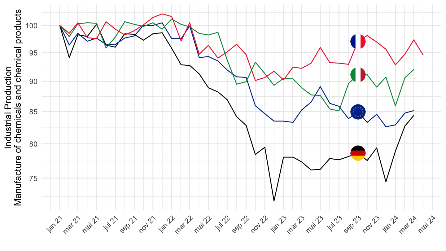
C2015 - Manufacture of fertilisers and nitrogen compounds
All
Code
sts_inpr_m %>%
  filter(nace_r2 == "C2015",
         unit == "I21",
         geo %in% c("FR", "DE", "IT", "EA20"),
         s_adj == "SCA") %>%
  select(geo, time, values) %>%
  group_by(geo) %>%
  mutate(values = 100*values/values[time == "2010M01"]) %>%
  left_join(geo, by = "geo") %>%
  mutate(Geo = ifelse(geo == "DE", "Germany", Geo)) %>%
  mutate(Geo = ifelse(geo == "EA20", "Europe", Geo)) %>%
  month_to_date %>%
  left_join(colors, by = c("Geo" = "country")) %>%
  ggplot() + ylab("Industrial Production") + xlab("") + theme_minimal() +
  geom_line(aes(x = date, y = values, color = color)) +
  scale_color_identity() + add_4flags +
  scale_x_date(breaks = seq(1920, 2100, 5) %>% paste0("-01-01") %>% as.Date,
               labels = date_format("%Y")) +
  theme(legend.position = "none") +
  scale_y_log10(breaks = seq(-60, 300, 10))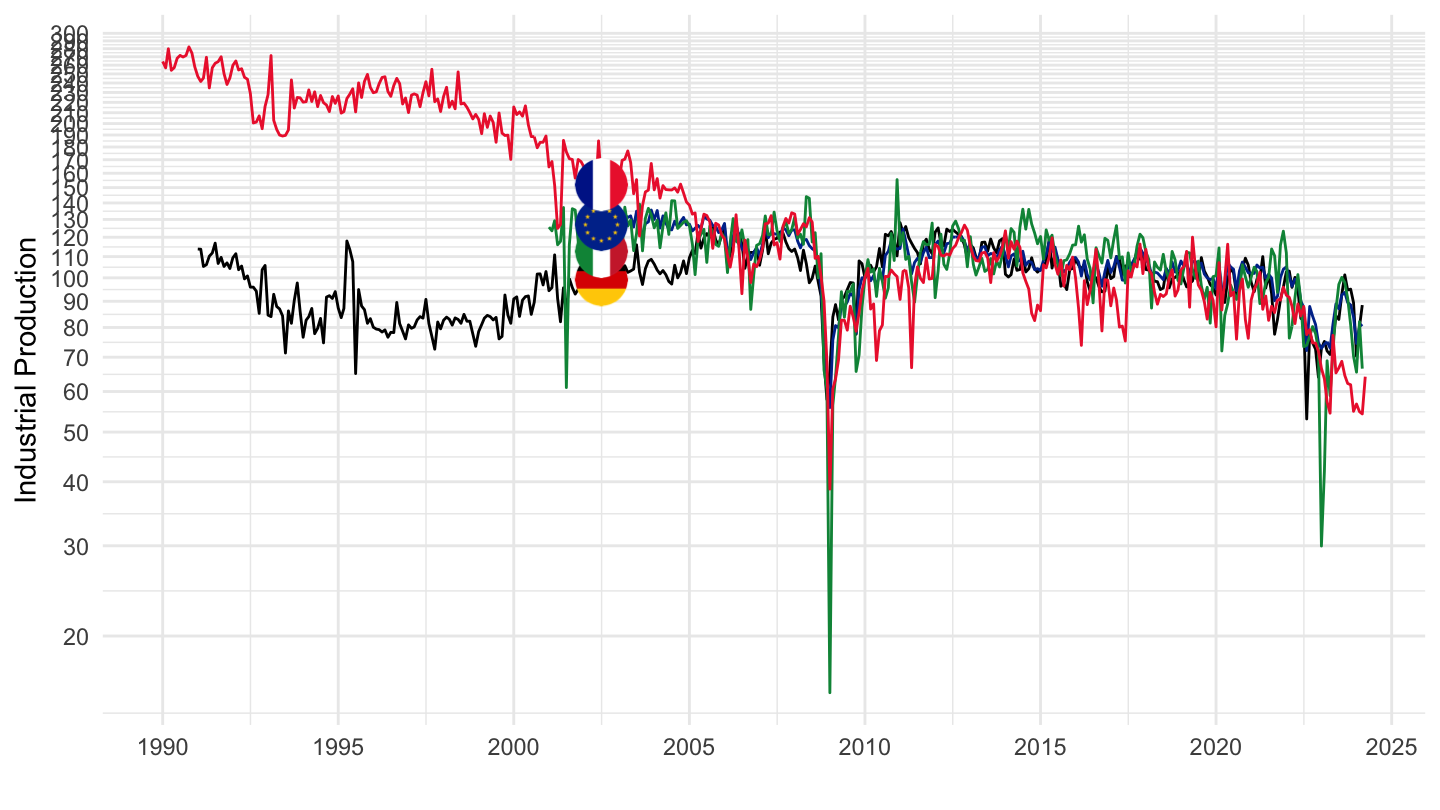
1992-
Code
sts_inpr_m %>%
  filter(nace_r2 == "C2015",
         unit == "I21",
         geo %in% c("FR", "DE", "IT", "EA20"),
         s_adj == "SCA") %>%
  select(geo, time, values) %>%
  left_join(geo, by = "geo") %>%
  mutate(Geo = ifelse(geo == "DE", "Germany", Geo)) %>%
  mutate(Geo = ifelse(geo == "EA20", "Europe", Geo)) %>%
  month_to_date %>%
  group_by(geo) %>%
  arrange(date) %>%
  mutate(values = 100*values/values[1]) %>%
  filter(date >= as.Date("1992-01-01")) %>%
  left_join(colors, by = c("Geo" = "country")) %>%
  ggplot() + ylab("Industrial Production") + xlab("") + theme_minimal() +
  geom_line(aes(x = date, y = values, color = color)) +
  scale_color_identity() + add_4flags +
  scale_x_date(breaks = seq(1920, 2100, 2) %>% paste0("-01-01") %>% as.Date,
               labels = date_format("%Y")) +
  theme(legend.position = "none") +
  scale_y_log10(breaks = seq(-60, 300, 10))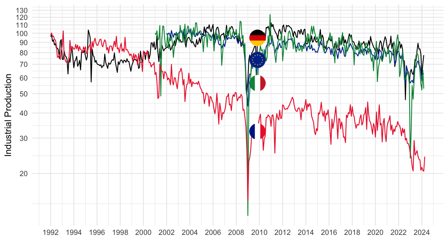
2000-
Code
sts_inpr_m %>%
  filter(nace_r2 == "C2015",
         unit == "I21",
         geo %in% c("FR", "DE", "IT", "EA20"),
         s_adj == "SCA") %>%
  select(geo, time, values) %>%
  left_join(geo, by = "geo") %>%
  mutate(Geo = ifelse(geo == "DE", "Germany", Geo)) %>%
  mutate(Geo = ifelse(geo == "EA20", "Europe", Geo)) %>%
  month_to_date %>%
  group_by(geo) %>%
  mutate(values = 100*values/values[1]) %>%
  filter(date >= as.Date("2000-01-01")) %>%
  left_join(colors, by = c("Geo" = "country")) %>%
  ggplot() + ylab("Industrial Production\nManufacture of fertilisers and nitrogen compounds") + xlab("") +
  geom_line(aes(x = date, y = values, color = color)) +
  scale_color_identity() + add_4flags + theme_minimal() +
  scale_x_date(breaks = seq(1920, 2100, 2) %>% paste0("-01-01") %>% as.Date,
               labels = date_format("%y")) +
  scale_y_log10(breaks = seq(-60, 300, 10))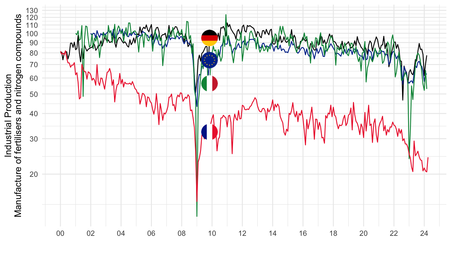
2019-
Code
sts_inpr_m %>%
  filter(nace_r2 == "C2015",
         unit == "I21",
         geo %in% c("FR", "DE", "IT", "EA20"),
         s_adj == "SCA") %>%
  select(geo, time, values) %>%
  group_by(geo) %>%
  mutate(values = 100*values/values[time == "2019M01"]) %>%
  left_join(geo, by = "geo") %>%
  mutate(Geo = ifelse(geo == "DE", "Germany", Geo)) %>%
  mutate(Geo = ifelse(geo == "EA20", "Europe", Geo)) %>%
  month_to_date %>%
  filter(date >= as.Date("2019-01-01")) %>%
  left_join(colors, by = c("Geo" = "country")) %>%
  ggplot() + ylab("Industrial Production\nManufacture of fertilisers and nitrogen compounds") + xlab("") +
  geom_line(aes(x = date, y = values, color = color)) +
  scale_color_identity() + add_4flags + theme_minimal() +
  scale_x_date(breaks = "3 months",
               labels = date_format("%b %y")) +
  add_4flags +
  theme(legend.position = "none",
        axis.text.x = element_text(angle = 45, vjust = 1, hjust = 1)) +
  scale_y_log10(breaks = seq(-60, 300, 10))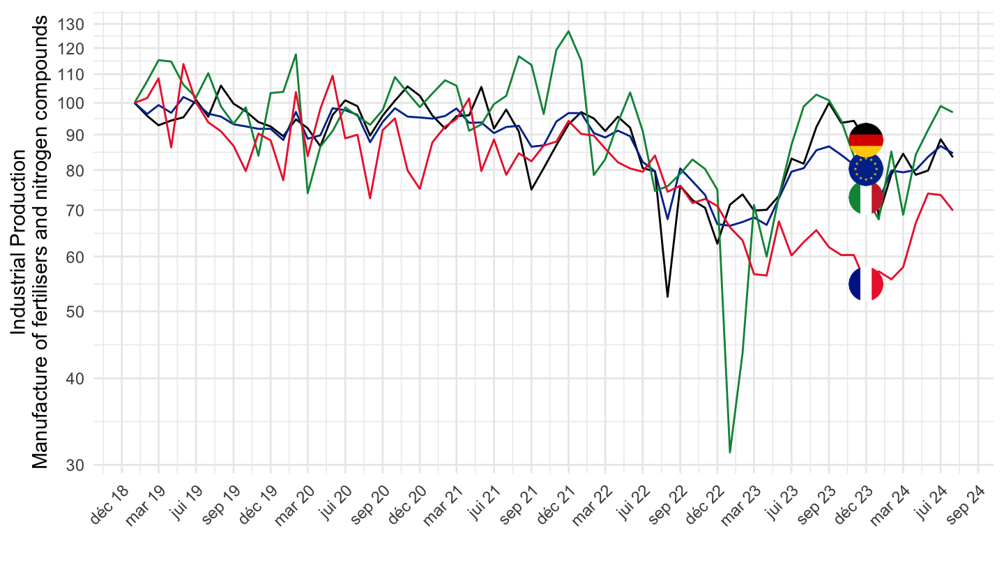
2020-
Code
sts_inpr_m %>%
  filter(nace_r2 == "C2015",
         unit == "I21",
         geo %in% c("FR", "DE", "IT", "EA20"),
         s_adj == "SCA") %>%
  select(geo, time, values) %>%
  group_by(geo) %>%
  mutate(values = 100*values/values[time == "2020M01"]) %>%
  left_join(geo, by = "geo") %>%
  mutate(Geo = ifelse(geo == "DE", "Germany", Geo)) %>%
  mutate(Geo = ifelse(geo == "EA20", "Europe", Geo)) %>%
  month_to_date %>%
  filter(date >= as.Date("2020-01-01")) %>%
  left_join(colors, by = c("Geo" = "country")) %>%
  ggplot() + ylab("Industrial Production\nManufacture of fertilisers and nitrogen compounds") + xlab("") +
  geom_line(aes(x = date, y = values, color = color)) +
  scale_color_identity() + add_4flags + theme_minimal() +
  theme(legend.position = "none",
        axis.text.x = element_text(angle = 45, vjust = 1, hjust = 1)) +
  scale_x_date(breaks = "2 months",
               labels = date_format("%b %y")) +
  scale_y_log10(breaks = seq(-60, 300, 10))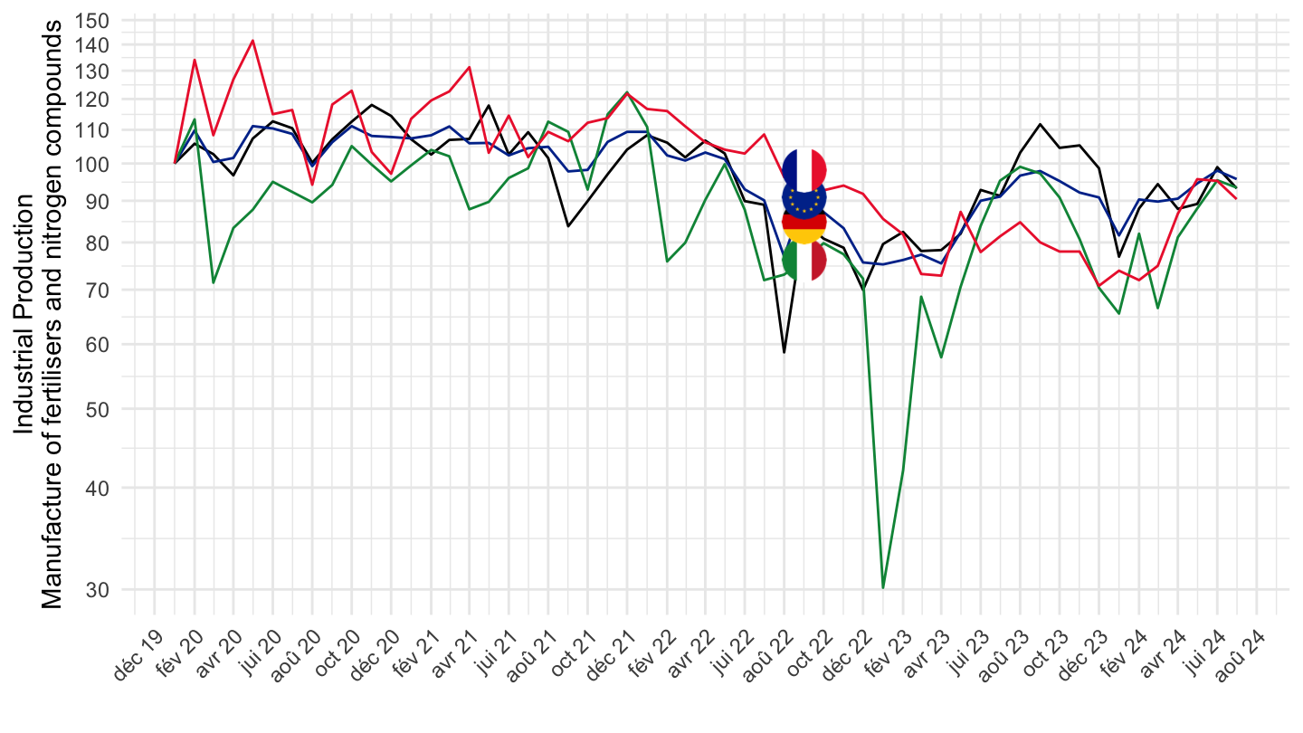
2021-
Code
load_data("eurostat/nace_r2_fr.RData")
sts_inpr_m %>%
  filter(nace_r2 == "C2015",
         unit == "I21",
         geo %in% c("FR", "DE", "IT", "EA20"),
         s_adj == "SCA") %>%
  group_by(geo) %>%
  mutate(values = 100*values/values[time == "2021M01"]) %>%
  left_join(geo, by = "geo") %>%
  left_join(nace_r2, by = "nace_r2") %>%
  mutate(Geo = ifelse(geo == "DE", "Germany", Geo)) %>%
  mutate(Geo = ifelse(geo == "EA20", "Europe", Geo)) %>%
  month_to_date %>%
  filter(date >= as.Date("2021-01-01")) %>%
  left_join(colors, by = c("Geo" = "country")) %>%
  ggplot() + ylab("Production industrielle\nFabrication de produits azotés et d'engrais") + xlab("") +
  geom_line(aes(x = date, y = values, color = color)) +
  scale_color_identity() + add_4flags + theme_minimal() +
  theme(legend.position = "none",
        axis.text.x = element_text(angle = 45, vjust = 1, hjust = 1)) +
  scale_x_date(breaks = "2 months",
               labels = date_format("%b %y")) +
  scale_y_log10(breaks = seq(-60, 300, 10))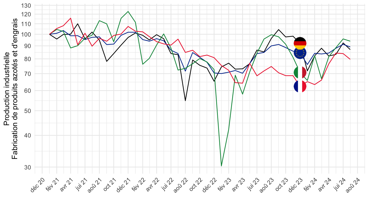
Manufacturing
All
Code
sts_inpr_m %>%
  filter(nace_r2 == "C",
         unit == "I21",
         geo %in% c("FR", "DE", "IT", "EA20"),
         s_adj == "SCA") %>%
  select(geo, time, values) %>%
  group_by(geo) %>%
  mutate(values = 100*values/values[time == "1997M01"]) %>%
  left_join(geo, by = "geo") %>%
  mutate(Geo = ifelse(geo == "DE", "Germany", Geo)) %>%
  mutate(Geo = ifelse(geo == "EA20", "Europe", Geo)) %>%
  month_to_date %>%
  left_join(colors, by = c("Geo" = "country")) %>%
  ggplot() + ylab("Industrial Production") + xlab("") + theme_minimal() +
  geom_line(aes(x = date, y = values, color = color)) +
  scale_color_identity() + add_4flags +
  scale_x_date(breaks = seq(1920, 2100, 5) %>% paste0("-01-01") %>% as.Date,
               labels = date_format("%Y")) +
  theme(legend.position = "none") +
  scale_y_log10(breaks = seq(-60, 300, 10))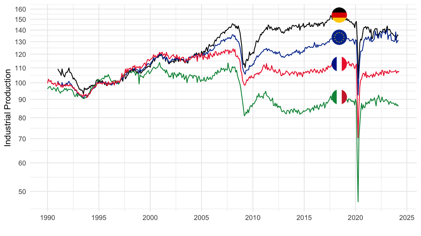
1992-
Code
sts_inpr_m %>%
  filter(nace_r2 == "C",
         unit == "I21",
         geo %in% c("FR", "DE", "IT", "EA20"),
         s_adj == "SCA") %>%
  select(geo, time, values) %>%
  group_by(geo) %>%
  month_to_date %>%
  arrange(date) %>%
  mutate(values = 100*values/values[1]) %>%
  left_join(geo, by = "geo") %>%
  mutate(Geo = ifelse(geo == "DE", "Germany", Geo)) %>%
  mutate(Geo = ifelse(geo == "EA20", "Europe", Geo)) %>%
  filter(date >= as.Date("1992-01-01")) %>%
  left_join(colors, by = c("Geo" = "country")) %>%
  ggplot() + ylab("Industrial Production") + xlab("") + theme_minimal() +
  geom_line(aes(x = date, y = values, color = color)) +
  scale_color_identity() + add_4flags +
  scale_x_date(breaks = seq(1920, 2100, 2) %>% paste0("-01-01") %>% as.Date,
               labels = date_format("%Y")) +
  theme(legend.position = "none") +
  scale_y_log10(breaks = seq(-60, 300, 10))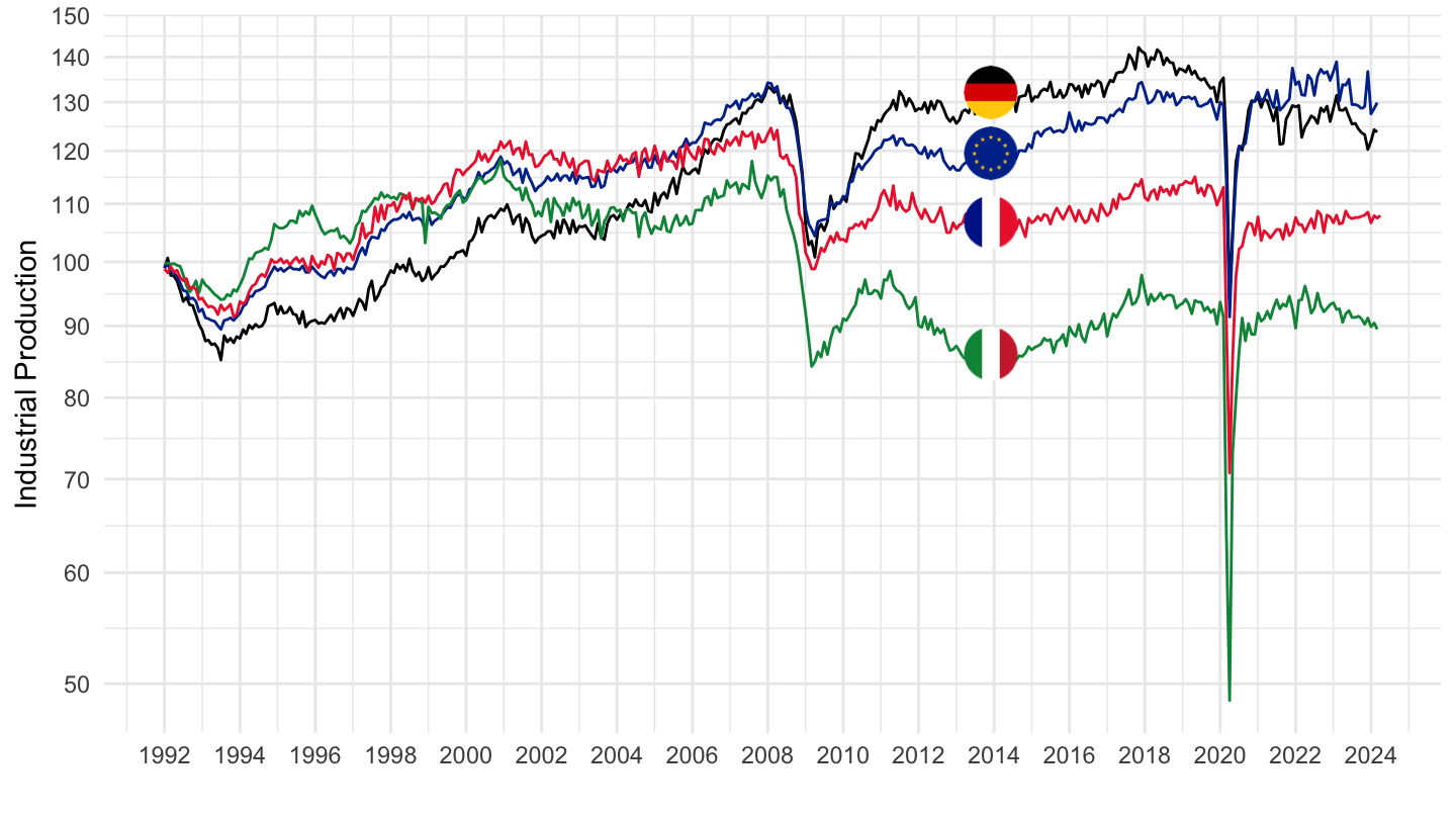
1995-
Code
sts_inpr_m %>%
  filter(nace_r2 == "C",
         unit == "I21",
         geo %in% c("FR", "DE", "IT", "EA20"),
         s_adj == "SCA") %>%
  select(geo, time, values) %>%
  group_by(geo) %>%
  month_to_date %>%
  filter(date >= as.Date("1995-01-01")) %>%
  arrange(date) %>%
  mutate(values = 100*values/values[1]) %>%
  left_join(geo, by = "geo") %>%
  mutate(Geo = ifelse(geo == "DE", "Germany", Geo)) %>%
  mutate(Geo = ifelse(geo == "EA20", "Europe", Geo)) %>%
  left_join(colors, by = c("Geo" = "country")) %>%
  ggplot() + ylab("Industrial Production") + xlab("") + theme_minimal() +
  geom_line(aes(x = date, y = values, color = color)) +
  scale_color_identity() +
  scale_x_date(breaks = seq(1920, 2100, 2) %>% paste0("-01-01") %>% as.Date,
               labels = date_format("%Y")) +
  add_4flags +
  scale_y_log10(breaks = seq(-60, 300, 10))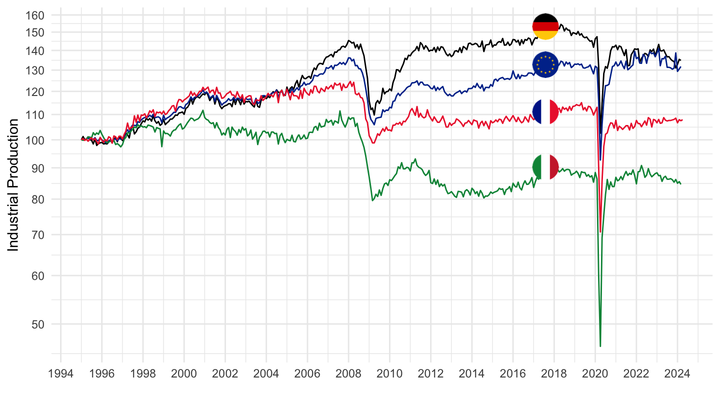
2000-
Code
sts_inpr_m %>%
  filter(nace_r2 == "C",
         unit == "I21",
         geo %in% c("FR", "DE", "IT", "EA20"),
         s_adj == "SCA") %>%
  select(geo, time, values) %>%
  group_by(geo) %>%
  month_to_date %>%
  filter(date >= as.Date("2000-01-01")) %>%
  arrange(date) %>%
  mutate(values = 100*values/values[1]) %>%
  left_join(geo, by = "geo") %>%
  mutate(Geo = ifelse(geo == "DE", "Germany", Geo)) %>%
  mutate(Geo = ifelse(geo == "EA20", "Europe", Geo)) %>%
  left_join(colors, by = c("Geo" = "country")) %>%
  ggplot() + ylab("Industrial Production") + xlab("") + theme_minimal() +
  geom_line(aes(x = date, y = values, color = color)) +
  scale_color_identity() +
  scale_x_date(breaks = seq(1920, 2100, 2) %>% paste0("-01-01") %>% as.Date,
               labels = date_format("%Y")) +
  add_4flags +
  scale_y_log10(breaks = seq(-60, 300, 10))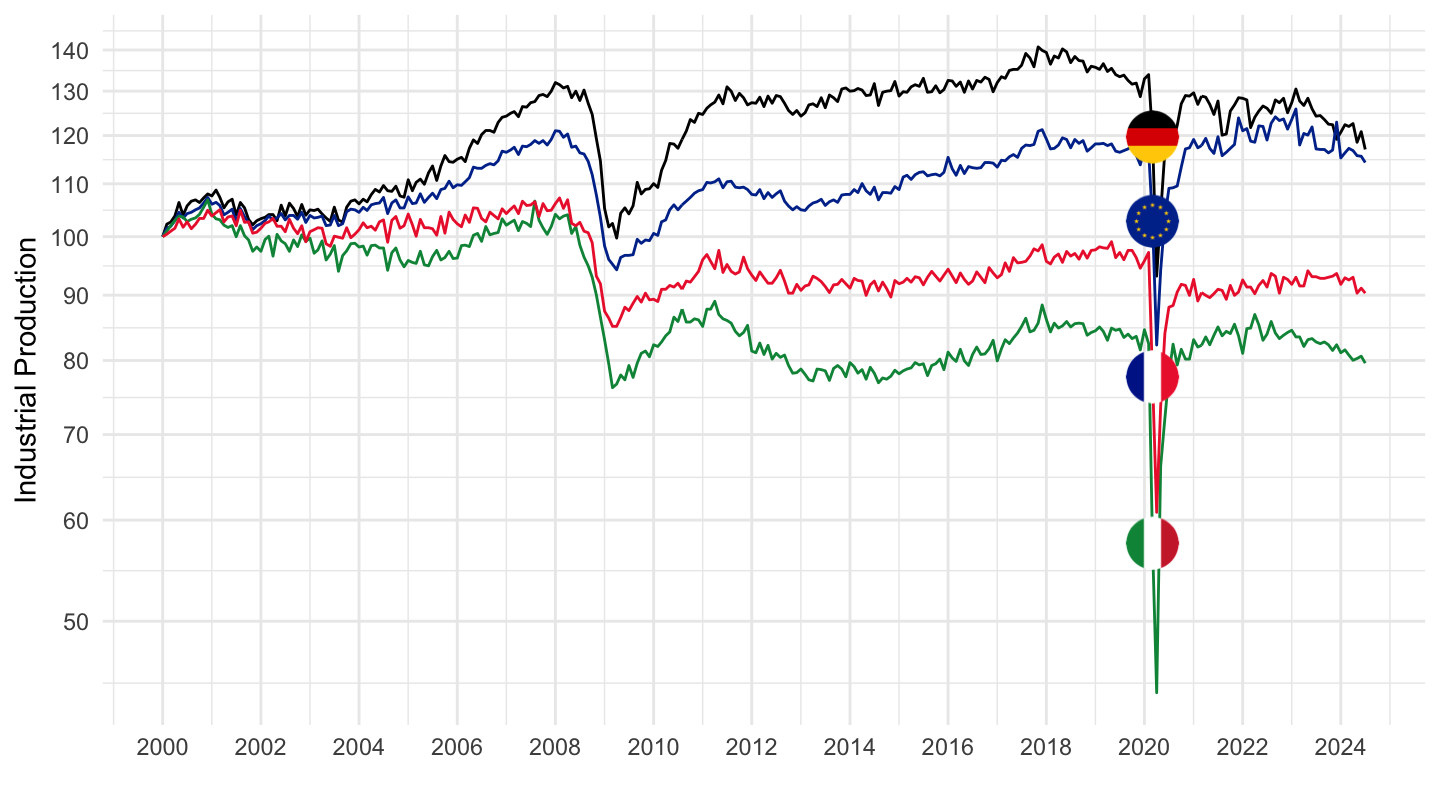
2019-
Code
sts_inpr_m %>%
  filter(nace_r2 == "C",
         unit == "I21",
         geo %in% c("FR", "DE", "IT", "EA20"),
         s_adj == "SCA") %>%
  select(geo, time, values) %>%
  group_by(geo) %>%
  mutate(values = 100*values/values[time == "2019M01"]) %>%
  left_join(geo, by = "geo") %>%
  mutate(Geo = ifelse(geo == "DE", "Germany", Geo)) %>%
  mutate(Geo = ifelse(geo == "EA20", "Europe", Geo)) %>%
  month_to_date %>%
  filter(date >= as.Date("2019-01-01")) %>%
  left_join(colors, by = c("Geo" = "country")) %>%
  ggplot() + ylab("Industrial Production") + xlab("") + theme_minimal() +
  geom_line(aes(x = date, y = values, color = color)) +
  scale_color_identity() +
  scale_x_date(breaks = "3 months",
               labels = date_format("%b %y")) +
  theme(legend.position = "none",
        axis.text.x = element_text(angle = 45, vjust = 1, hjust = 1)) +
  add_4flags +
  theme(legend.position = "none") +
  scale_y_log10(breaks = seq(-60, 300, 10))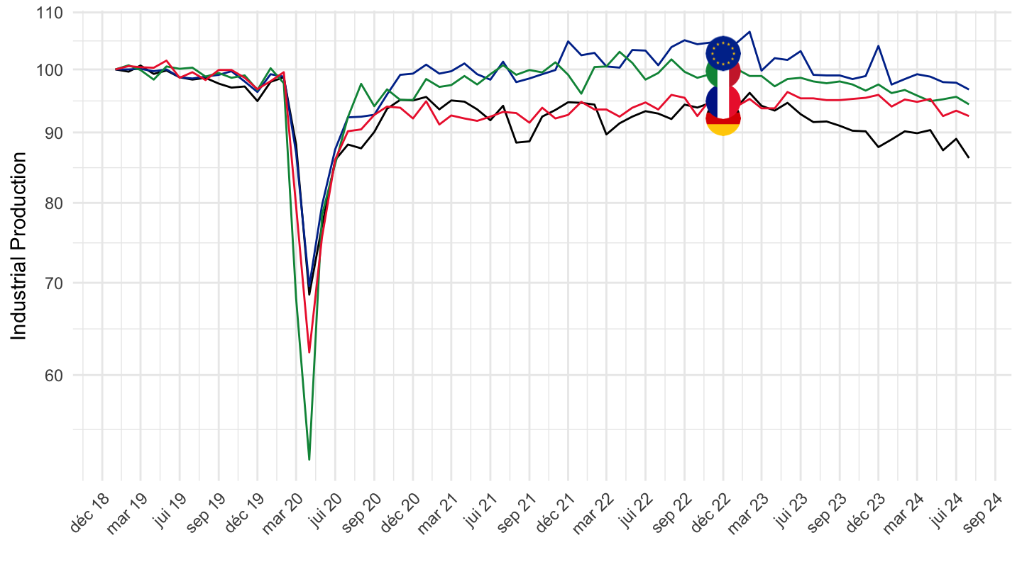
2020-
Code
sts_inpr_m %>%
  filter(nace_r2 == "C",
         unit == "I21",
         geo %in% c("FR", "DE", "IT", "EA20", "ES"),
         s_adj == "SCA") %>%
  select(geo, time, values) %>%
  group_by(geo) %>%
  mutate(values = 100*values/values[time == "2020M02"]) %>%
  left_join(geo, by = "geo") %>%
  mutate(Geo = ifelse(geo == "DE", "Germany", Geo)) %>%
  mutate(Geo = ifelse(geo == "EA20", "Europe", Geo)) %>%
  month_to_date %>%
  filter(date >= as.Date("2020-02-01")) %>%
  left_join(colors, by = c("Geo" = "country")) %>%
  ggplot() + ylab("Industrial Production, Manufacturing") + xlab("") + theme_minimal() +
  geom_line(aes(x = date, y = values, color = color)) +
  scale_color_identity() + add_5flags +
  theme(legend.position = "none",
        axis.text.x = element_text(angle = 45, vjust = 1, hjust = 1)) +
  scale_x_date(breaks = "2 months",
               labels = date_format("%b %y")) +
  scale_y_log10(breaks = seq(-60, 300, 10))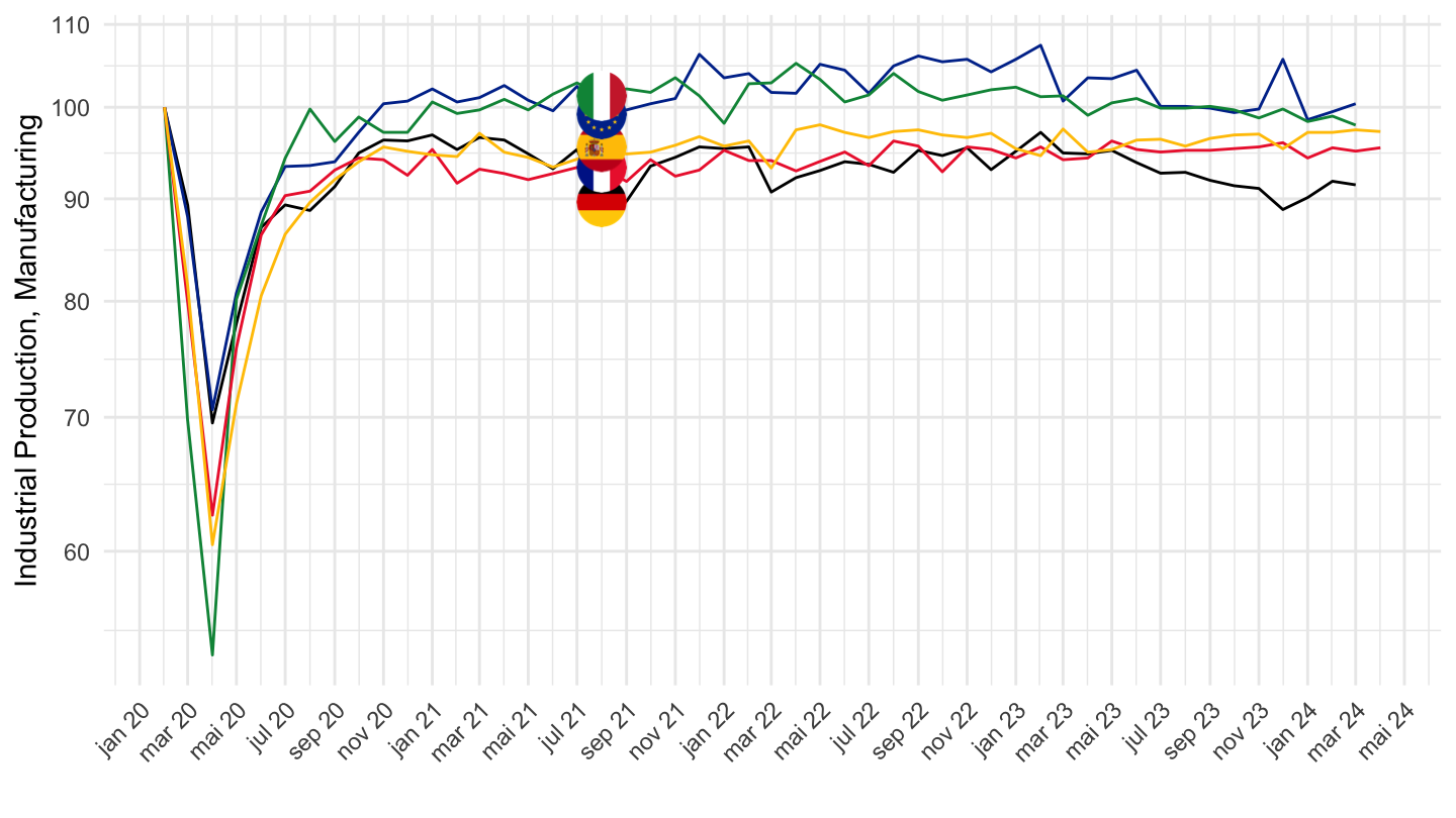
Covid-19
Table
Code
sts_inpr_m %>%
  filter(nace_r2 == "C",
         unit == "I21",
         s_adj == "SCA",
         time %in% c("2019M11", "2020M02", "2020M03", "2020M04", "2020M05", "2020M08", "2020M11"),
         !(geo %in% c("IE", "EU28"))) %>%
  select(geo, time, values) %>%
  group_by(geo) %>%
  mutate(values = 100*values/values[time == "2019M11"]) %>%
  left_join(geo, by = "geo") %>%
  spread(time, values) %>%
  mutate(Geo = ifelse(geo == "DE", "Germany", Geo)) %>%
  mutate(Flag = gsub(" ", "-", str_to_lower(Geo)),
         Flag = paste0('<img src="../../bib/flags/vsmall/', Flag, '.png" alt="Flag">')) %>%
  select(Flag, everything()) %>%
  arrange(`2020M04`) %>%
  {if (is_html_output()) datatable(., filter = 'top', rownames = F, escape = F) else .}
2018
Code
sts_inpr_m %>%
  filter(nace_r2 == "C",
         unit == "I21",
         geo %in% c("FR", "DE", "IT"),
         s_adj == "SCA") %>%
  select(geo, time, values) %>%
  group_by(geo) %>%
  mutate(values = 100*values/values[time == "2018M01"]) %>%
  left_join(geo, by = "geo") %>%
  mutate(Geo = ifelse(geo == "DE", "Germany", Geo)) %>%
  month_to_date %>%
  filter(date >= as.Date("2018-01-01")) %>%
  ggplot() + ylab("Industrial Production") + xlab("") + theme_minimal() +
  geom_line(aes(x = date, y = values, color = Geo)) +
  scale_color_manual(values = c("#0055a4", "#000000", "#008c45")) +
  scale_x_date(breaks = "3 months",
               labels = date_format("%b %y")) +
  geom_image(data = . %>%
               filter(date == as.Date("2021-01-01")) %>%
               mutate(image = paste0("../../icon/flag/", str_to_lower(Geo), ".png")),
             aes(x = date, y = values, image = image), asp = 1.5) +
  theme(legend.position = "none",
        axis.text.x = element_text(angle = 45, vjust = 1, hjust = 1)) +
  scale_y_log10(breaks = seq(-60, 300, 10))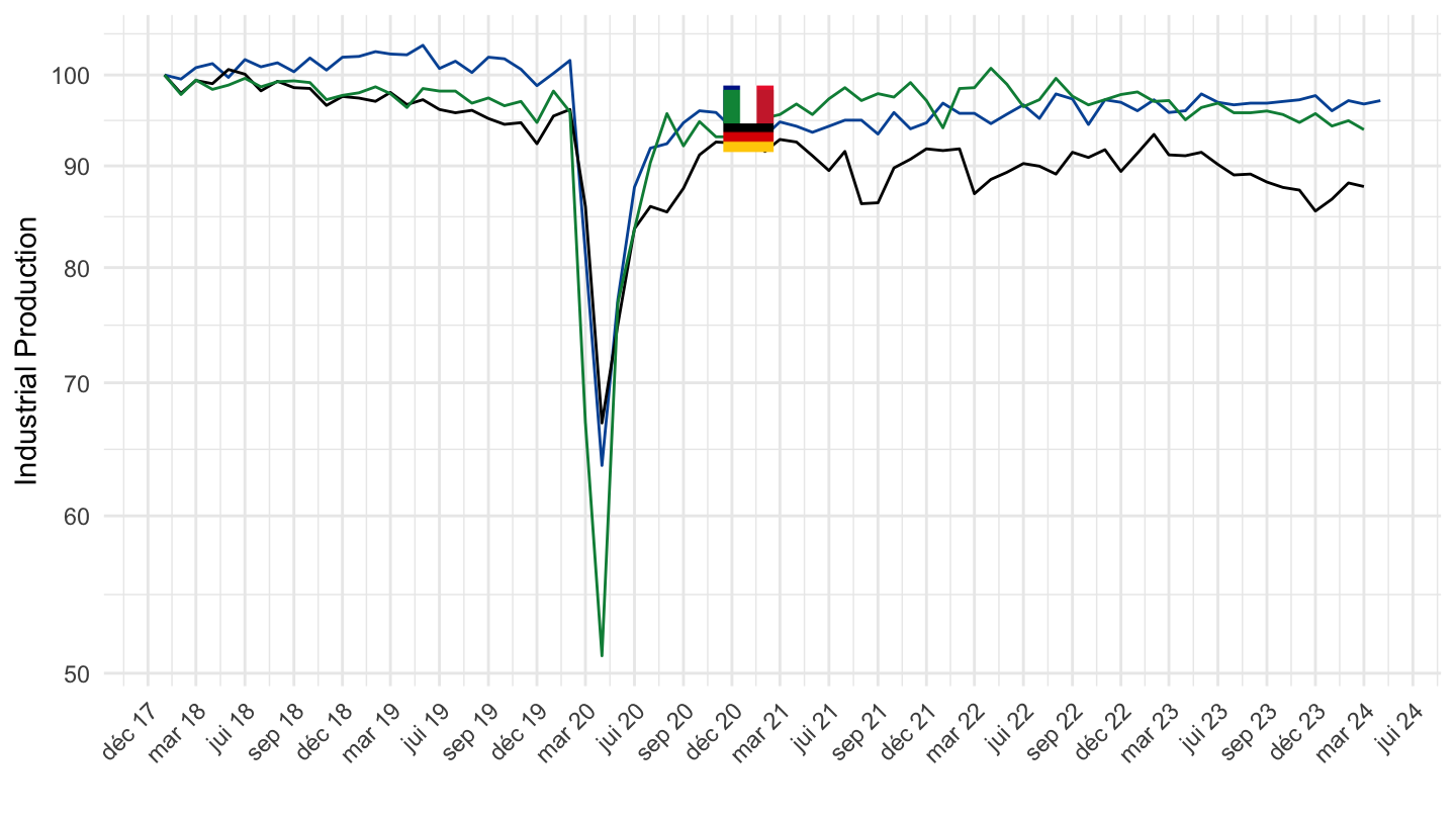
2019M09
Code
sts_inpr_m %>%
  filter(nace_r2 == "C",
         unit == "I21",
         geo %in% c("FR", "DE", "IT"),
         s_adj == "SCA") %>%
  select(geo, time, values) %>%
  group_by(geo) %>%
  mutate(values = 100*values/values[time == "2019M09"]) %>%
  left_join(geo, by = "geo") %>%
  mutate(Geo = ifelse(geo == "DE", "Germany", Geo)) %>%
  month_to_date %>%
  filter(date >= as.Date("2019-09-01")) %>%
  ggplot() + ylab("Industrial Production") + xlab("") + theme_minimal() +
  geom_line(aes(x = date, y = values, color = Geo)) +
  scale_color_manual(values = c("#0055a4", "#000000", "#008c45")) +
  scale_x_date(breaks = "2 months",
               labels = date_format("%b %y")) +
  geom_image(data = . %>%
               filter(date == as.Date("2021-05-01")) %>%
               mutate(image = paste0("../../icon/flag/", str_to_lower(Geo), ".png")),
             aes(x = date, y = values, image = image), asp = 1.5) +
  theme(legend.position = "none",
        axis.text.x = element_text(angle = 45, vjust = 1, hjust = 1)) +
  scale_y_log10(breaks = seq(-60, 300, 10))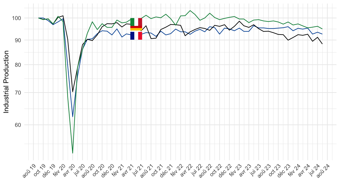
2020M02
Code
sts_inpr_m %>%
  filter(nace_r2 == "C",
         unit == "I21",
         geo %in% c("FR", "DE", "IT", "ES"),
         s_adj == "SCA") %>%
  select(geo, time, values) %>%
  group_by(geo) %>%
  mutate(values = 100*values/values[time == "2020M02"]) %>%
  left_join(geo, by = "geo") %>%
  mutate(Geo = ifelse(geo == "DE", "Germany", Geo)) %>%
  month_to_date %>%
  filter(date >= as.Date("2020-02-01")) %>%
  ggplot() + ylab("Industrial Production") + xlab("") + theme_minimal() +
  geom_line(aes(x = date, y = values, color = Geo)) +
  scale_color_manual(values = c("#0055a4", "#000000", "#008c45", "#C60B1E")) +
  scale_x_date(breaks = "3 months",
               labels = date_format("%b %y")) +
  geom_image(data = . %>%
               filter(date == as.Date("2020-08-01")) %>%
               mutate(image = paste0("../../icon/flag/", str_to_lower(Geo), ".png")),
             aes(x = date, y = values, image = image), asp = 1.5) +
  theme(legend.position = "none",
        axis.text.x = element_text(angle = 45, vjust = 1, hjust = 1)) +
  scale_y_log10(breaks = seq(-60, 300, 10))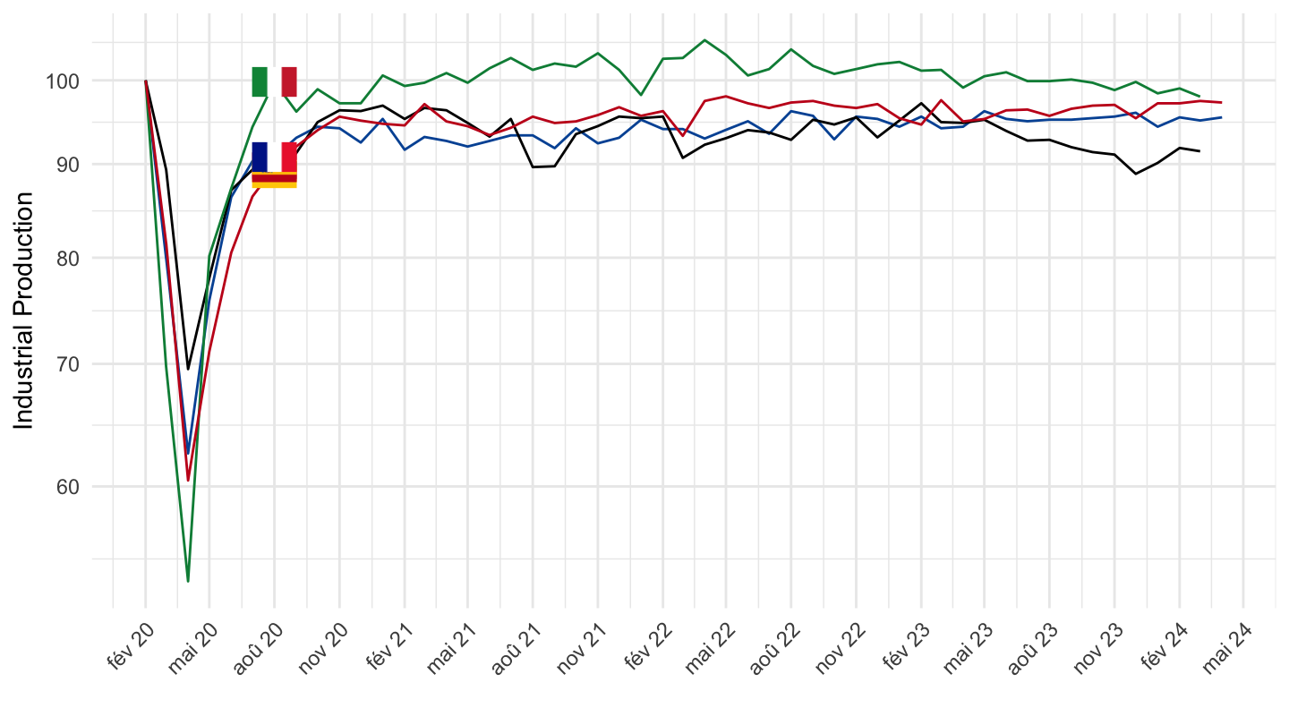
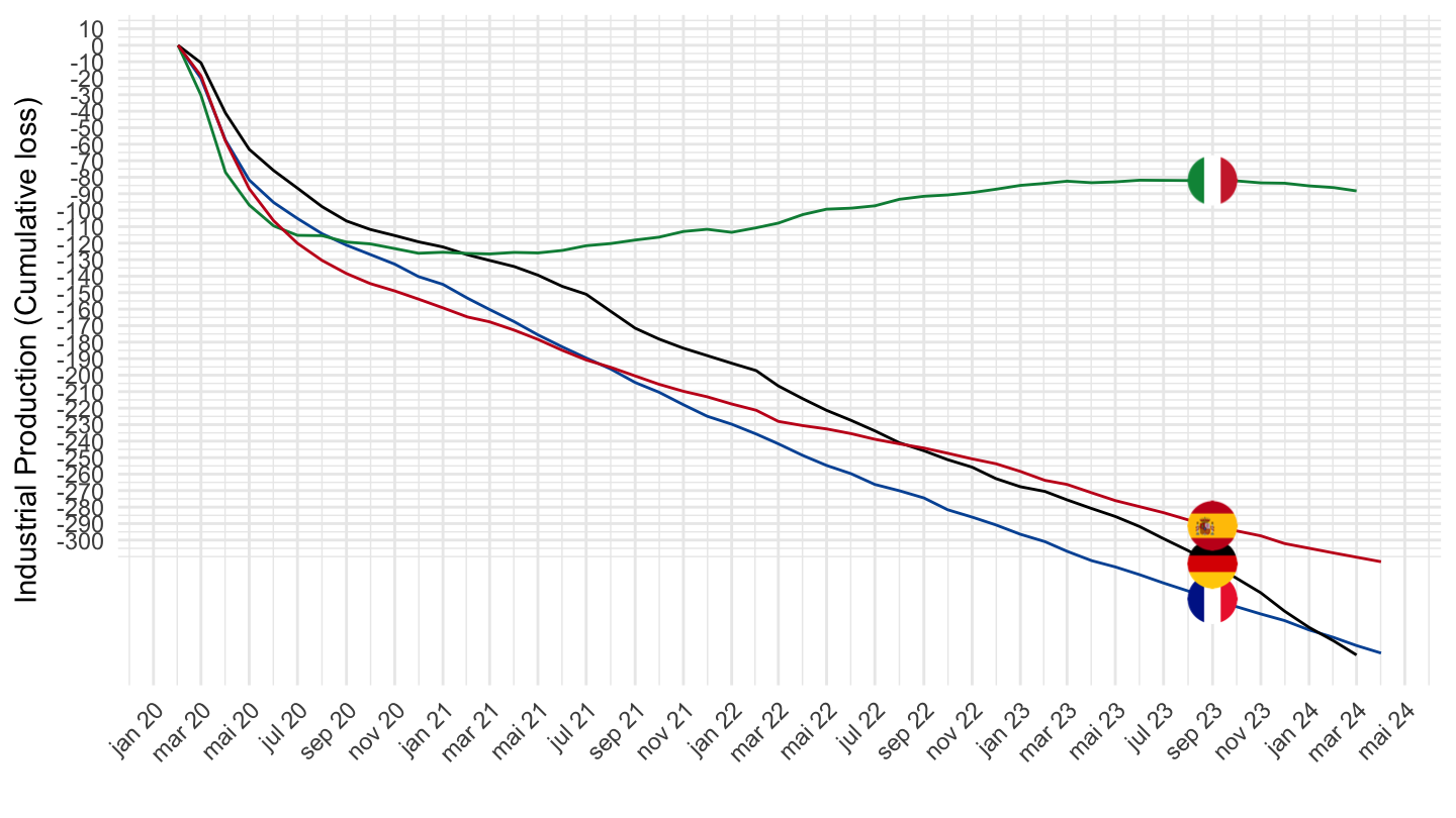
Cumulative loss in production
Code
sts_inpr_m %>%
  filter(nace_r2 == "C",
         unit == "I21",
         geo %in% c("FR", "DE", "IT", "ES", "UK"),
         s_adj == "SCA") %>%
  select(geo, time, values) %>%
  group_by(geo) %>%
  mutate(values = 100*values/values[time == "2020M02"]) %>%
  left_join(geo, by = "geo") %>%
  month_to_date %>%
  filter(date >= as.Date("2020-02-01")) %>%
  group_by(Geo) %>%
  arrange(date) %>%
  mutate(values = values-100,
         values = cumsum(values)) %>%
  left_join(colors, by = c("Geo" = "country")) %>%
  ggplot() + ylab("Industrial Production (Cumulative loss)") + xlab("") + theme_minimal() +
  geom_line(aes(x = date, y = values, color = color)) +
  scale_color_identity() +
  scale_x_date(breaks = "2 months",
               labels = date_format("%b %y")) +
  add_5flags +
  theme(legend.position = "none",
        axis.text.x = element_text(angle = 45, vjust = 1, hjust = 1)) +
  scale_y_continuous(breaks = seq(-300, 300, 10))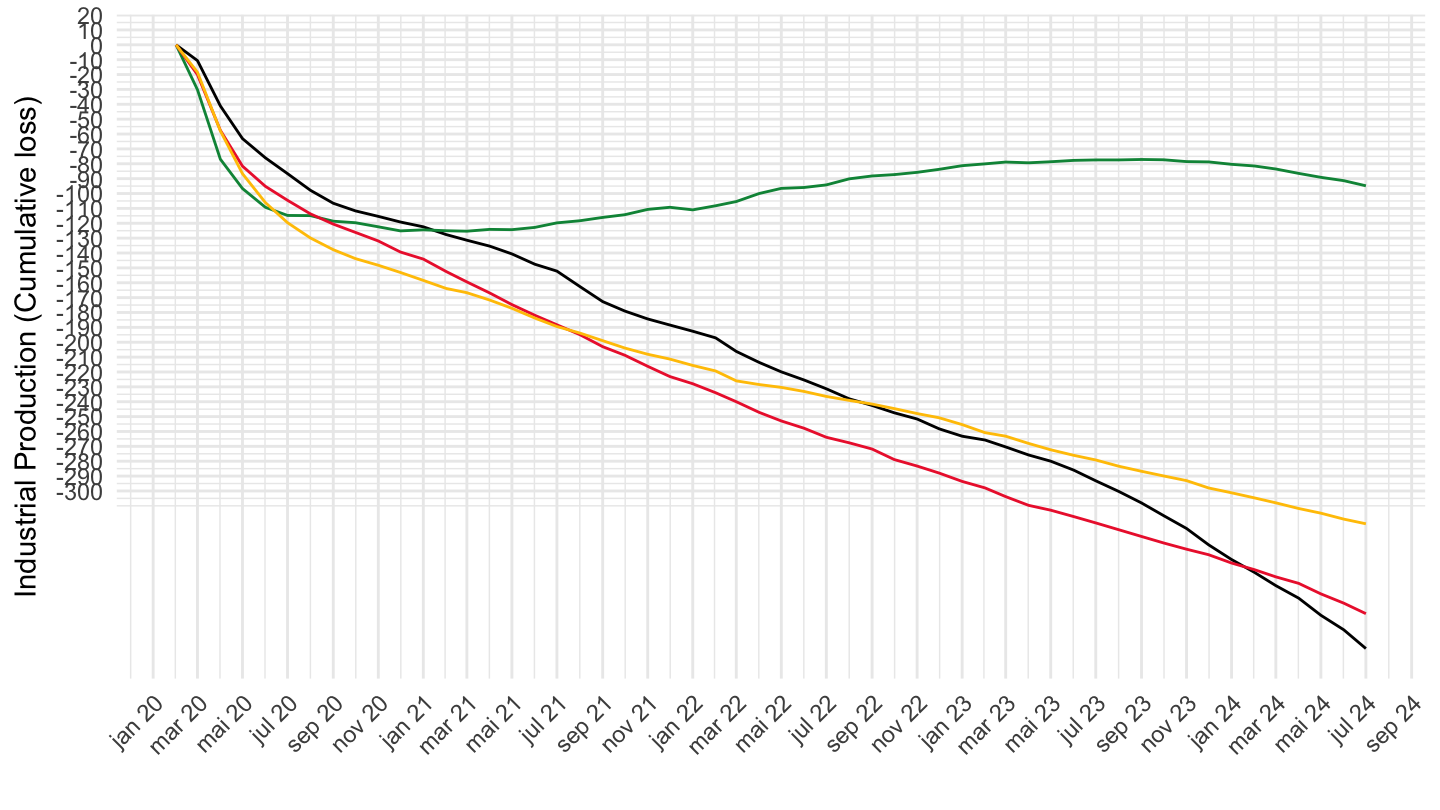
Cumulative loss in production
Code
sts_inpr_m %>%
  filter(nace_r2 == "C",
         unit == "I21",
         geo %in% c("FR", "DE", "IT", "ES"),
         s_adj == "SCA") %>%
  select(geo, time, values) %>%
  group_by(geo) %>%
  mutate(values = 100*values/values[time == "2020M02"]) %>%
  left_join(geo, by = "geo") %>%
  month_to_date %>%
  filter(date >= as.Date("2020-02-01")) %>%
  group_by(Geo) %>%
  arrange(date) %>%
  mutate(values = values-100,
         values = cumsum(values)) %>%
  ggplot() + ylab("Industrial Production (Cumulative loss)") + xlab("") + theme_minimal() +
  geom_line(aes(x = date, y = values, color = Geo)) +
  scale_color_manual(values = c("#0055a4", "#000000", "#008c45", "#C60B1E")) +
  scale_x_date(breaks = "2 months",
               labels = date_format("%b %y")) +
  add_4flags +
  theme(legend.position = "none",
        axis.text.x = element_text(angle = 45, vjust = 1, hjust = 1)) +
  scale_y_continuous(breaks = seq(-300, 300, 10))