Last observation: déc. 2015 (N = 902) · 2015 (N = 2223)
First observation: 1990 (N = 1148) · janv. 1990 (N = 302)
Last data update: 24 oct. 2026, 02:11
Last compile: 24 oct. 2026, 03:26
`IPC-1998` |>
  group_by(TITLE_FR, IDBANK) |>
  summarise(Nobs = n()) |>
  arrange(-Nobs) |>
print_table_conditional()`IPC-1998` |>
group_by(REF_AREA) |>
summarise(Nobs = n()) |>
arrange(-Nobs) |>
print_table_conditional()| REF_AREA | Nobs |
|---|---|
| FE | 162501 |
| FM | 93015 |
| D971 | 5544 |
| D972 | 5544 |
| D973 | 5544 |
| D974 | 5544 |
`IPC-1998` |>
  group_by(TIME_PERIOD) |>
  summarise(Nobs = n()) |>
  arrange(desc(TIME_PERIOD)) |>
print_table_conditional()`IPC-1998` |>
filter(IDBANK %in% c("000641339", "000641338")) %>%
mutate(TITLE_FR = TITLE_FR %>% gsub("Indice mensuel d'inflation sous-jacente - Base 1998 - ", "", .),
TITLE_FR = TITLE_FR %>% gsub("- Corrigé des mesures fiscales et des variations saisonnières - Série arrêtée", "", .)) |>
month_to_date() |>
ggplot() +
geom_line(aes(x = date, y = OBS_VALUE, color = TITLE_FR, linetype = TITLE_FR)) +
scale_color_manual(values = viridis(5)[1:4]) +
theme_minimal() +
scale_x_date(breaks = seq(1920, 2100, 5) |> paste0("-01-01") |> as.Date(),
labels = date_format("%Y")) +
theme(legend.position = c(0.75, 0.3),
legend.title = element_blank()) +
scale_y_log10(breaks = seq(0, 200, 10),
labels = dollar_format(accuracy = 1, prefix = "")) +
ylab("Indice des prix") + xlab("")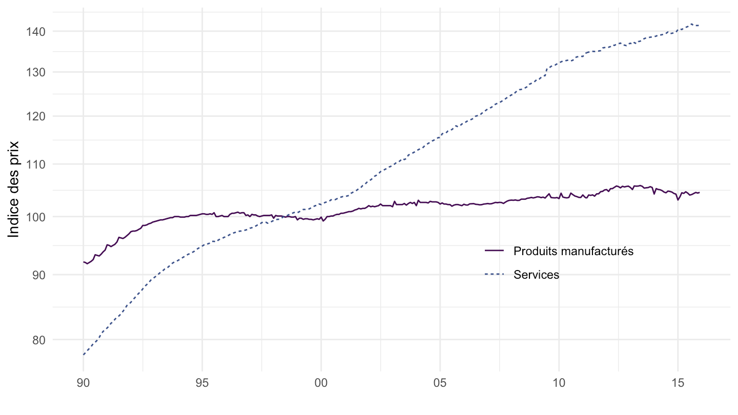
`IPC-1998` |>
  filter(NATURE == "POND",
         REF_AREA == "FM",
         TIME_PERIOD %in% c("1998", "1996", "1994", "1992", "1990", "2005", "2010", "2002"),
         MENAGES_IPC == "ENSEMBLE") |>
  select_if(function(col) length(unique(col)) > 1) |>
  select(-IDBANK, -TITLE_FR, -TITLE_EN, -OBS_STATUS, -OBS_TYPE) |>
  spread(TIME_PERIOD, OBS_VALUE) |>
print_table_conditional()`IPC-1998` |>
filter(INDICATEUR == "IPC",
MENAGES_IPC == "ENSEMBLE",
COICOP1998 %in% c("1253"),
REF_AREA == "FM",
NATURE == "POND") |>
year_to_date() |>
mutate(OBS_VALUE = OBS_VALUE/10000) |>
ggplot() + ylab("Poids de l'assurance santé dans l'indice des prix") + xlab("") + theme_minimal() +
geom_line(aes(x = date, y = OBS_VALUE)) +
scale_color_manual(values = viridis(3)[1:2]) +
scale_x_date(breaks = seq(1920, 2100, 1) |> paste0("-01-01") |> as.Date(),
labels = date_format("%Y")) +
scale_y_continuous(breaks = 0.01*seq(0, 10, 0.1),
labels = percent_format(accuracy = .1))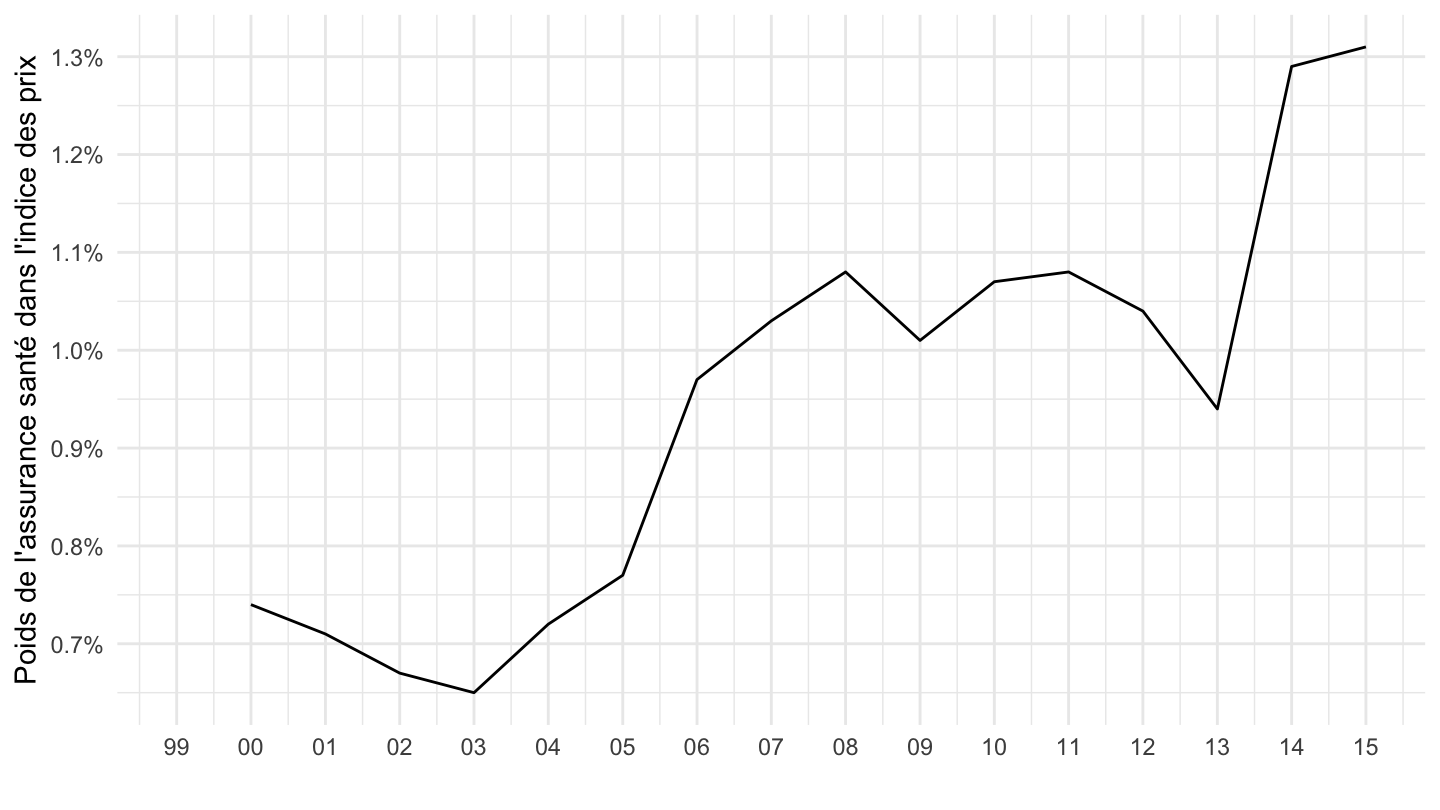
`IPC-1998` |>
  filter(INDICATEUR == "IPC",
         MENAGES_IPC == "ENSEMBLE",
         COICOP1998 %in% c("0221"),
         REF_AREA == "FM",
         NATURE == "POND") |>
  year_to_date() |>
  mutate(OBS_VALUE = OBS_VALUE/10000) |>
  ggplot() + ylab("Poids du tabac dans l'indice des prix") + xlab("") + theme_minimal() +
  geom_line(aes(x = date, y = OBS_VALUE)) +
  scale_color_manual(values = viridis(3)[1:2]) +
  scale_x_date(breaks = seq(1920, 2100, 1) |> paste0("-01-01") |> as.Date(),
               labels = date_format("%Y")) +
  scale_y_continuous(breaks = 0.01*seq(0, 10, 0.1),
                     labels = percent_format(accuracy = .1))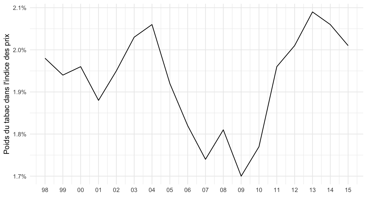
`IPC-1998` |>
  filter(INDICATEUR == "IPC",
         MENAGES_IPC == "ENSEMBLE",
         COICOP1998 %in% c("06"),
         REF_AREA == "FM",
         NATURE == "POND") |>
  year_to_date() |>
  mutate(OBS_VALUE = OBS_VALUE/10000) |>
  ggplot() + ylab("Poids de la santé dans l'indice des prix") + xlab("") + theme_minimal() +
  geom_line(aes(x = date, y = OBS_VALUE)) +
  scale_color_manual(values = viridis(3)[1:2]) +
  scale_x_date(breaks = seq(1920, 2100, 1) |> paste0("-01-01") |> as.Date(),
               labels = date_format("%Y")) +
  scale_y_continuous(breaks = 0.01*seq(0, 12, 0.1),
                     labels = percent_format(accuracy = .1))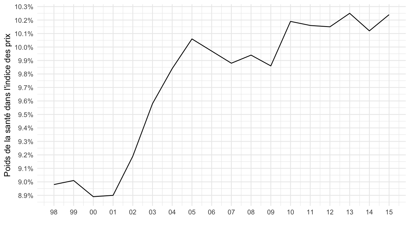
`IPC-1998` |>
  filter(COICOP1998 %in% c("00", "02", "11", "04"),
         REF_AREA == "FM",
         NATURE == "INDICE",
         FREQ == "M") |>
  month_to_date() |>
  group_by(COICOP1998) |>
  arrange(date) |>
  mutate(OBS_VALUE = 100*OBS_VALUE/OBS_VALUE[1]) |>
  ggplot() + ylab("Indice des prix") + xlab("") + theme_minimal() +
  geom_line(aes(x = date, y = OBS_VALUE, color = Coicop1998)) +
  scale_color_manual(values = viridis(5)[1:4]) +
  scale_x_date(breaks = seq(1920, 2100, 2) |> paste0("-01-01") |> as.Date(),
               labels = date_format("%Y")) +
  theme(legend.position = c(0.3, 0.85),
        legend.title = element_blank()) +
  scale_y_log10(breaks = c(100, 120, 150, 200, 220, 250, 300, 400, 500),
                     labels = dollar_format(accuracy = 1, prefix = ""))
`IPC-1998` |>
  filter(COICOP1998 %in% c("00", "10", "07", "12"),
         REF_AREA == "FM",
         NATURE == "INDICE",
         FREQ == "M") |>
  month_to_date() |>
  group_by(COICOP1998) |>
  arrange(date) |>
  mutate(OBS_VALUE = 100*OBS_VALUE/OBS_VALUE[1]) |>
  ggplot() + ylab("Indice des prix") + xlab("") + theme_minimal() +
  geom_line(aes(x = date, y = OBS_VALUE, color = Coicop1998)) +
  scale_color_manual(values = viridis(5)[1:4]) +
  scale_x_date(breaks = seq(1920, 2100, 2) |> paste0("-01-01") |> as.Date(),
               labels = date_format("%Y")) +
  theme(legend.position = c(0.3, 0.85),
        legend.title = element_blank()) +
  scale_y_log10(breaks = seq(100, 300, 10),
                     labels = dollar_format(accuracy = 1, prefix = ""))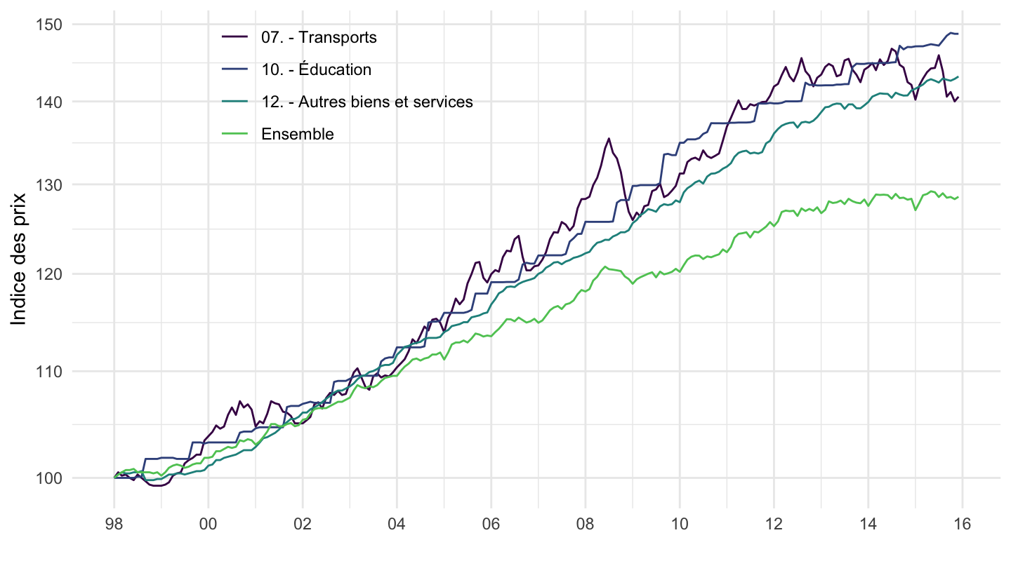
`IPC-1998` |>
  filter(COICOP1998 %in% c("00", "05", "01", "03"),
         REF_AREA == "FM",
         NATURE == "INDICE",
         FREQ == "M") |>
  month_to_date() |>
  group_by(COICOP1998) |>
  arrange(date) |>
  mutate(OBS_VALUE = 100*OBS_VALUE/OBS_VALUE[1]) |>
  ggplot() + ylab("Indice des prix") + xlab("") + theme_minimal() +
  geom_line(aes(x = date, y = OBS_VALUE, color = Coicop1998)) +
  scale_color_manual(values = viridis(5)[1:4]) +
  scale_x_date(breaks = seq(1920, 2100, 2) |> paste0("-01-01") |> as.Date(),
               labels = date_format("%Y")) +
  theme(legend.position = c(0.3, 0.85),
        legend.title = element_blank()) +
  scale_y_log10(breaks = seq(100, 300, 10),
                     labels = dollar_format(accuracy = 1, prefix = ""))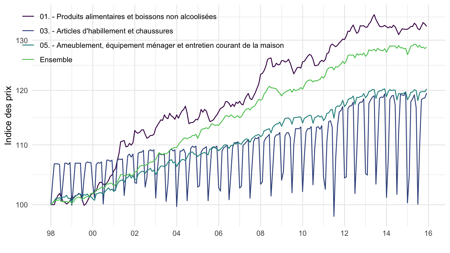
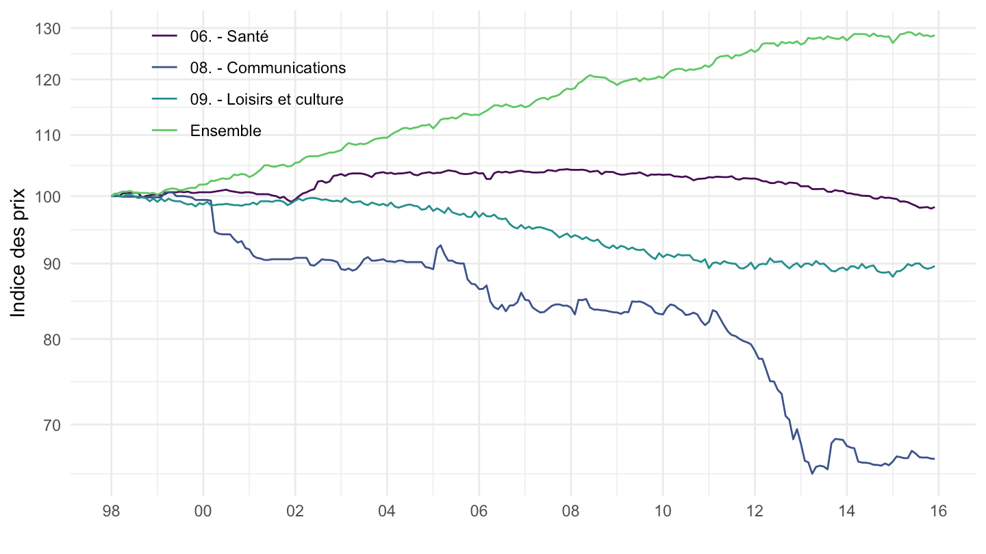
`IPC-1998` |>
  filter(COICOP1998 %in% c("00", "06", "09", "08"),
         REF_AREA == "FM",
         NATURE == "INDICE",
         FREQ == "M") |>
  month_to_date() |>
  group_by(COICOP1998) |>
  arrange(date) |>
  mutate(OBS_VALUE = 100*OBS_VALUE/OBS_VALUE[1]) |>
  ggplot() + ylab("Indice des prix") + xlab("") + theme_minimal() +
  geom_line(aes(x = date, y = OBS_VALUE, color = Coicop1998)) +
  scale_color_manual(values = viridis(5)[1:4]) +
  scale_x_date(breaks = seq(1920, 2100, 2) |> paste0("-01-01") |> as.Date(),
               labels = date_format("%Y")) +
  theme(legend.position = c(0.2, 0.85),
        legend.title = element_blank()) +
  scale_y_log10(breaks = seq(10, 300, 10),
                     labels = dollar_format(accuracy = 1, prefix = ""))